Highlights
What are the main findings?
- Provide an overview of current developments, challenges, and future directions for remote sensing effects and invariants studies.
- Synthesize disparate remote sensing effects and invariants under a unified framework.
What are the implications of the main findings?
- Provide an understanding of the characterization, principles, and potential applications of selected remote sensing effects and invariants.
- Initiate theoretical exploration of the fundamental principles in remote sensing science.
Abstract
Remote sensing is a technique to acquire information from a distance. Remote sensing effects refer to any factors that need to be considered in remote sensing processes, while remote sensing invariants represent features that remain stable throughout these processes. Both remote sensing effects and invariants are fundamental to the study of remote sensing systems, methods, algorithms, products, and applications. Many studies have explored different effects and invariants independently, yet these studies are scattered across the literature and a comprehensive synthesis is lacking within the community. This paper intends to synthesize various remote sensing effects and invariants under a unified framework. The characterization, underlying principles, and potential applications of a selected group of remote sensing effects were first examined. Subsequently, a suite of nine key effects, atmospheric effects, background effects, clumping effects, directional effects, heterogeneity effects, saturation effects, scaling effects, temporal effects, and topographic effects, were addressed. Furthermore, a list of remote sensing invariants, including spectral, spatial, temporal, directional, and thematical invariants, were analyzed. Potential directions for future studies were further discussed. This synthesis represents a concerted effort to advance the theoretical understanding of fundamental principles in remote sensing science.
1. Introduction
Remote sensing obtains information about Earth from a distance without any physical contact with the target. The characteristics of the information received from a sensor, whether near-surface, airborne, or spaceborne, depend on many factors, particularly, the reflectance or emittance of the target, the nature and magnitude of the atmosphere, the topography of the ground, and the geometry of the sun–target–sensor system. Consequently, our capability to retrieve information is determined by these factors, collectively referred to as remote sensing effects.
There is no commonly agreed-upon definition for a “remote sensing effect” since “effect” itself is a very broad term. It can be generally defined as any factor, phenomenon, or event that needs to be considered via remote sensing processes. In theory, it is difficult to disentangle all effects, since many of them are closely entangled with each other. However, there are some effects that are critical for obtaining high-quality information and have been widely studied. These effects will be the focus of this paper. In addition to remote sensing effects, there are also some features that remain essentially unchanged during remote sensing data analysis. This property has been commonly utilized in parameter retrieval, where some parameters are kept invariant when deriving other variables. One such example is the pseudo-invariant calibration sites (PICS) commonly used in radiometric calibration [1,2], where the radiation properties of the sites are assumed to be invariant over time. Remote sensing effects and invariants exist in all aspects of remote sensing studies, including satellite-measured radiance, radiative transfer (RT) process, physical parameter retrieval, and product validation and applications. Although many studies have covered various effects and invariants individually, there is currently no comprehensive synthesis of remote sensing effects and invariants.
The objective of this paper is to provide an overview of various remote sensing effects and invariants under a unified framework. This study classifies and synthetically analyzes current progress, challenges, and future prospects in the study of remote sensing effects and invariants. The ultimate goal is to advocate for a synthetic study of these concepts and to advance theoretical remote sensing studies. Section 2 offers a synthetic analysis of different remote sensing effects, while Section 3 provides an overview of nine selected remote sensing effects. It is not our intention to present an exhaustive description of all known effects; for more comprehensive information, readers should refer to the cited references for each effect. Section 4 provides some general views on how to suppress, characterize, and accommodate various effects in remote sensing studies. Section 5 explores remote sensing invariants. Section 6 concludes the paper.
2. Characterization of Remote Sensing Effects
2.1. Remote Sensing Effects in Various Links
A large number of remote sensing effects have been proposed and investigated (Appendix A). They vary in different degrees of completeness and advancement. The remote sensing process can be treated as a chain of events or steps leading to a final output [3]. Remote sensing effects play distinct roles throughout this chain, beginning with the electromagnetic (EM) data source, such as solar radiation, thermal emission, and active EM radiation (LiDAR or radar). The illumination effect indicates the properties of the EM radiation and the distribution of luminance over the sky, whether it is directionally uniform or varies with weather conditions. The properties of the target, such as material composition, homogeneity, roughness, water content, salinity, temperature, texture, reflectance and emittance, and anisotropy properties are central to remote sensing signal processing. Moreover, the relative position and motion state of targets will cause radiance differences in different wavelengths. The location, altitude, and environmental conditions, such as disease, draught, dust, and fire, can also impact remote sensing data acquisition.
In field biophysical measurements, optical instruments, such as digital hemispherical photography (DHP), are affected by exposure setting, blooming, and vignetting effects, segment size, file format, and environmental contamination [4]. LAI-2200 (LI-COR, Lincoln, NE, USA), a standard field leaf area index (LAI) measurement instrument, is particularly susceptible to the ring effect [5]. For LiDAR measurements, the occlusion and saturation effects must be considered [6]. Woody and non-green element effects also require attention in LAI measurements using DHP, LAI-2200, and LiDAR. In general, all field measurements are subject to sampling effects, whether random, systematic, or stratified.
Satellite remote sensing is influenced by many effects, such as sensor spectral wavelength, spectral response, sensitivity, field-of-view, radiometric, spatial and spectral resolutions, active or passive observation modes, observation geometry, temporal variation, and orbital shift, among others. Recent studies have found that most land products derived from MODIS are affected by the orbital drift, especially for the fraction of absorbed photosynthetically active radiation (FAPAR) because of variations in solar illumination angle and light conditions [7].
Remote sensing models simulate the RT process in the atmosphere and vegetation systems. Typically, the radiation is decomposed into direct and diffuse components. The models need to account for photon interactions with the atmospheric and vegetation elements. The understory or background soil plays an important role in vegetation remote sensing, especially for a sparse canopy. For a water surface, the air–water interface effect must be considered in RT simulations of coupled air–water systems. Polarization effects are explicitly incorporated in polarized RT models [8,9].
Many factors affect remote sensing data storage, processing, and transmission. Data compression prior to transmission or storage may reduce data quality and lose critical details. Transmission delays or partial data loss from communication issues can result in incomplete or outdated datasets. In image classification, different classifiers may introduce varying uncertainties in final products. Image interpretation inherently involves artificial effects that may cause systematic errors. Scale differences, temporal coherence, and spectral consistency disparities between remote sensing products and reference data can introduce errors in product evaluation and applications.
2.2. Connections Among Remote Sensing Effects
Remote sensing effects are not isolated phenomena but are instead interconnected with each other. Some effects exhibit similarities or equivalences and can be studied collectively, while others demonstrate opposing characteristics. These relationships are broadly categorized as follows.
2.2.1. Generic and Integrated Effects
Generic effects are fundamental effects that should be considered across multiple aspects of remote sensing studies. The scaling effect is one such example that exists in field measurements, satellite observations, product generation and evaluation, and applications. Another example is the temporal effect, which affects instruments, targets, observers, and environmental conditions. In contrast to generic effects, certain effects hold particular importance in specific applications. These effects are also more independent, such as the texture effect, which is commonly used for image classification. The clumping effect, while predominantly significant at local scales, may also contribute at the landscape and regional scales [10].
Integrated effects refer to the combined results from the interaction and synergy of multiple individual effects. Many effects are an integration of several sub-effects. Spatial and temporal effects are commonly analyzed together as spatio-temporal effects. Temporal effects are usually combined with variations in spectral, angular, and textural characteristics. The adjacency effect is a combination of atmospheric and surface effects, while one of them may play a primary role and the other a secondary. In mountainous areas, topographic effects are coupled with atmospheric and directional effects in affecting surface reflectance estimation and land cover classification [11,12,13].
2.2.2. Equivalent, Facilitating, and Neutralizing Effects
Equivalent effects are essentially similar ones that produce the same, interchangeable outcome. Many effects are literally equivalent. For example, both phenology and seasonal effects are similar to each other and are subcategories of temporal effects. Directional effects are closely related to angular effects, sun glint effects, specular effects, non-Lambertian effects, hotspot and darkspot effects, shading effects, and others.
Some effects (facilitating effects) mutually reinforce each other in remote sensing studies, while others (neutralizing effects) may counterbalance each other. Leaf biochemical components (e.g., chlorophyll content) and canopy structural properties (e.g., LAI) jointly influence canopy reflectance, which makes it difficult to decouple them in parameter retrieval [14]. Similarly, canopy clumping, woody components, and non-green foliage collectively complicate LAI retrieval from optical remote sensing. In practice, clumping and woody effects may be compensated for in forest LAI estimation [10,15].
2.2.3. Beneficial and Detrimental Effects
Depending on the user’s purpose, remote sensing effects can be either beneficial or detrimental. Beneficial effects are positive and desirable for a user; for example, temporal effects are valuable for time-series analysis and thematic classification. Many effects are beneficial and can be utilized in remote sensing studies. The usefulness of an effect depends on the purpose of the application. Traditional visual interpretation and digital classification have long capitalized on spatial patterns, spectral characteristics, and temporal variations, while temporal effects have been commonly utilized for global land cover classification [16].
Detrimental effects cause negative and complicated results for a user. For a coupled atmosphere and surface system, the atmospheric influence hinders surface detection, and vice versa. A satellite pixel, especially those of moderate-to-coarse resolution (e.g., MODIS), may contain a mixture of different components; each has its own directional reflectance, thus making pixel reflectance modeling particularly challenging. Thermally emitted radiance from any surface depends on surface temperature and emissivity; estimating either one requires accounting for their mutual dependence.
3. Overview of Selected Remote Sensing Effects
This section focuses on a selected group of nine effects that have received significant attention in land surface remote sensing. These effects are well-defined and have been extensively studied in the literature. Their key characteristics are summarized below with examples and references.
3.1. Atmospheric Effect
Atmosphere effects are the joint result of all kinds of atmospheric components, such as atmospheric molecules, aerosols, water vapor, ozone, methane, carbon monoxide, nitrous oxide, and carbon dioxide [17]. The main atmospheric effects include scattering, absorption, cloud cover, aerosol, water vapor, refraction, and thermal effects. Atmospheric effects modify signals received by sensors on satellites or other platforms, making it challenging to interpret data accurately without compensating for them. Atmospheric conditions also impact optical instruments used for canopy biophysical structural measurements, such as DHP, LAI-2200, and AccuPAR (METER Group, Pullman, WA, USA). Therefore, diffuse conditions are generally recommended for optimal performance, particularly for forests, to avoid the impact of direct irradiance [18,19,20]. Among these instruments, DHP has been found to be more robust due to its lower sensitivity to illumination conditions [21].
Atmospheric correction techniques aim to remove or reduce atmospheric distortions so that true surface parameters can be more accurately retrieved [22]. Atmospheric corrections enhance image quality and improve classification accuracy [23]. Numerous studies have reviewed and evaluated atmospheric correction methods [24,25,26]. Aerosols and water vapor, which exhibit greater spatial and temporal variability than other atmospheric components, introduce significant uncertainties in atmospheric correction. Therefore, accurately characterizing these components is essential for effective atmospheric correction. Various filtering approaches have been developed to process remote sensing data contaminated by atmospheric effects [27,28,29]. Combining data from multiple bands or using images acquired at different times can help mitigate the atmospheric influence. Specialized vegetation indices (VIs), such as the atmospherically resistant vegetation index (ARVI) [30] and infrared simple ratio (ISR) [31], were developed to minimize atmospheric impacts.
Physical modeling [32] and deep learning methods [33] are also used to provide processing solutions for all kinds of illumination conditions. Atmospheric models, such as MODTRAN [34] and 6S [35], are commonly used to simulate and compensate for the effects of scattering, absorption, and other atmospheric phenomena. Based on these models, some software packages such as ATmospheric CORrection (ATCOR3) [36], the Landsat Surface Reflectance Code (LaSRC) [37], and Sen2Cor implemented in SeNtinel’s Application Platform (Sen2Cor-SNAP) [38] were developed to perform atmospheric correction for high-resolution images. However, atmospheric correction may not be necessary for classification and change detection applications when training data and target data maintain consistent relative scales [39].
Validation of atmospheric correction results is crucial to ensure that the processed remote sensing data accurately represent surface reflectance or radiance. Field-measured surface reflectance data such as those from SpecNet [40] and HyperNav [41] are thus critical in validation of the corrected data. When there are no concurrent field measurements, atmospheric parameters derived from satellite images can be used to reconstruct atmospheric conditions and verify corrections [42,43]. By combining visual inspection, quantitative analysis, and cross-validation, one can ensure that atmospheric correction improves data accuracy for downstream applications like land cover classification and environmental monitoring.
3.2. Background Effect
Background effects refer to the mixture of both target and background information in the sensor. Background effects primarily arise from soil, snow, understory, or water backgrounds. In forest environments, the background may refer to all the materials below the canopy such as understory plants, leaf litter, grasses, lichens, mosses, rocks, soil, snow, water, or their mixtures [44,45]. Typically, in forests, a moss or lichen layer covers the ground surface beneath grasses. Similarly, in agricultural fields, a thin weed layer commonly exists beneath the main crop canopy.
Background materials influence vegetation canopy reflectance and VIs, consequently affecting canopy parameter retrieval. Indeed, the background effect on the canopy reflectance decreases with an increasing LAI (Figure 1). Combining information from different bands can eliminate some background effects and significantly enhance canopy information extraction. Several VIs have been specifically developed for this purpose, including the soil-adjusted vegetation index (SAVI) [46], the modified soil-adjusted vegetation index (MSAVI) [47], the reduced simple ratio (RSR) [48], and the normalized difference phenology index (NDPI) [49].
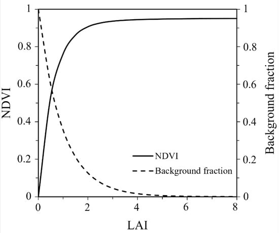
Figure 1.
Variation of the normalized difference vegetation index (NDVI) and the background fraction with leaf area index (LAI) simulated from the PROSAIL canopy reflectance model [50].
Forest background information can be retrieved from remote sensing techniques, especially from multiangle sensors such as CASI and MISR [45,51,52]. In canopy reflectance models, background contributions are represented in different schemes [53,54,55]. For example, the MODIS LAI algorithm uses 25 patterns of effective ground reflectance to parameterize the contribution of sub-canopy surface (soil and/or understory) [56]. In practice, background characteristics for low-to-medium density forests are usually considered similar within a geographical area, although local variations may occur between adjacent stands of different densities [57]. When the overstory coverage is high (e.g., >70%), the background has little effect on canopy reflectance and albedo [58].
The background reflectance estimated from remote sensing can be used to retrieve the overstory parameters [59]. However, the background information retrieval in forests may be partly influenced by non-green materials in the canopy (trunks and branches) [60]. For dense forests (e.g., LAI > 4), there is no ability to retrieve background reflectivity (Figure 1). Furthermore, separating different understory components is still difficult; the model-retrieved background reflectance may not represent the true ground conditions but is more like an effective value from model inversion [61,62].
More attention is necessary for complicated snow backgrounds [63,64]. However, it is challenging to map a snow-covered area using optical satellite sensors, particularly during snowmelt [65]. A normalized difference snow index (NDSI) has been used to identify whether a snow or ice background is present [66]. On the other hand, snow cover benefits wintertime forest LAI estimation from airborne imagery by providing a uniformly bright background for hemispherical image analysis [64,67].
3.3. Clumping Effect
Canopy clumping effects characterize the spatial distribution of leaves or needles within a vegetation canopy, which is critical in determining the transmission and interception of light and precipitation [10,68,69]. Canopy clumping effects are usually quantified using the canopy clumping index (CI), defined as the ratio of the effective LAI (LAIe) to the true LAI. In landscape ecology, an aggregation index has also been used to measure the spatial aggregation of ecological adjacencies and class patches [70,71,72].
The CI can be estimated in the field using direct, indirect optical, and allometric methods [10]. Direct methods derive the CI by separately estimating LAIe and LAI. Indirect methods estimate the CI through the analysis of canopy gap fractions, while allometric methods use relationships with other biophysical parameters. Both passive optical sensors and active LiDAR systems, including terrestrial, airborne, and spaceborne platforms, have been successfully applied for CI estimation, following similar principles to field measurements [73,74]. Currently, most global CI products are generated through empirical relationships with the normalized difference hotspot and darkspot (NDHD) index derived from POLDER, MODIS, and MISR data [75,76,77].
Clumping effects are scale-dependent and tend to intensify with higher spatial resolution [78,79]. For broadleaf forests, foliage clumping patterns vary at within-crown and between-crown scales. For coniferous forests, foliage clumping can be described at the shoot, branch, crown, and landscape levels [10]. Clumping effects generally increase (decreasing CI value) with view elevation angle and canopy height, primarily due to the presence of larger gaps in the upper canopy compared to in the lower canopy. Seasonally, canopy clumping is more pronounced during the peak growing season compared to early and later growing periods [77].
The clumping effect significantly influences LAI field measurements, remote sensing modeling, and parameter retrieval and should be considered in canopy reflectance and land surface models. Partitioning the total LAI into sunlit and shaded components using the CI enhanced the estimation of gross primary production (GPP) [80], solar-induced fluorescence (SIF) [81], and surface evaporation [82,83]. Seasonal clumping variations have been used to explore their effects on canopy radiation absorption and GPP dynamics [84,85]. However, the interannual clumping variability has not been fully considered in current land surface models for climate change studies. Future studies should focus on implementing automated wireless measurement techniques, developing advanced remote sensing estimation methods, enhancing fundamental understanding of clumping characteristics, and improving clumping parameterization in land surface models.
3.4. Directional Effect
Directional effects represent variations in object properties with angles, such as variations in solar illumination, surface characteristics, and observed radiances. The surface directional effect is an intrinsic surface property and is crucial for the modeling and estimation of land surface properties. Directional effects are a sub-category of geometric effects, which are affected by Earth’s shape and rotation, sun-target-sensor configurations, terrain influences, and geo-reference projection [86]. The surface directional property is typically characterized by the bidirectional reflectance factor (BRF) and bidirectional reflectance distribution function (BRDF), which can be measured using various instruments in the field [87] or derived from remote sensing data [88]. Quantitative metrics such as the anisotropic factor [89], anisotropy index [90], and anisotropic flat index [91] are proposed to quantify surface reflectance anisotropy.
Correcting directional effects is particularly important for time-series analysis and the generation of long-term data records [92,93]. The influence of directional effects propagates from surface reflectance to VIs and therefore impacts the estimation of canopy biophysical variables such as LAI from observed reflectance and VIs. Commonly used VIs such as the normalized difference vegetation index (NDVI) and enhanced vegetation index (EVI) have suppressed directional effects to some extent but may still contain significant angular signatures [94]. In addition to VIs, BRDF normalization methods are frequently used to mitigate directional effects [95]. The effect of BRDF normalization depends on surface heterogeneity, model complexity, and model parameterization. Various canopy reflectance models have been developed to characterize these directional variations [53,96,97]. The MODIS processing chain, for instance, employs a kernel-driven BRDF model to produce nadir BRDF-adjusted reflectance (NBAR) products [88,98].
Consideration of directional effects is important due to the strong non-Lambertian scattering properties of vegetation surfaces and the directional influence of model parameters on the canopy reflectance [96]. Multi-angle observations generally improve LAI retrieval accuracy compared to single-angle measurements [99,100], as demonstrated by the MODIS LAI product derived from directional reflectance data [56,101]. Some researchers have suggested using angularly normalized or directionally based VIs for LAI estimation [102,103,104]. However, the magnitude of angular effects decreases with increasing LAI values, and the usage of angular properties for biophysical parameter retrieval diminishes for higher LAI [105].
Satellite observations acquired at off-nadir viewing angles inherently incorporate directional effects. A few satellite instruments like MODIS and MISR provide multi-angular views, but their ground sampling areas vary for different pixels within an image. For vegetation canopy, directional gap distribution represents another crucial directional property that is obtainable through photographic (e.g., DHP) and radiometric (e.g., LAI-2200) methods [106] and warrants further study.
3.5. Heterogeneity Effect
Heterogeneity effects refer to the mixing of different objects within a study target, for example, mixed pixels in land surface classification. Surface heterogeneity complicates surface classification, RT modeling, and biophysical parameter retrieval and validation. Properly addressing it is essential for accurate interpretation of surface properties. Surface heterogeneity effects are scale-dependent and are directly related to the sensor resolution. The greater the spatial detail registered in an image, the greater its sensitivity in detecting the internal variations in different categories contained in a larger pixel [107].
Comprehensive characterization of the heterogeneity effect needs to account for both horizontal and vertical dimensions. For vegetation canopies, the surface mixture of vegetation and soil can be expressed by the fractional vegetation cover (FVC), which is usually determined along transects in field measurements [108]. In the vertical direction, heterogeneity mainly stems from variations in biophysical and biochemical properties throughout the canopy profile. Foliage area density profiles can be measured with various vertical sampling methods [109]. LiDAR and radar sensors are particularly effective for capturing three-dimensional heterogeneity patterns [110]. Both horizontal and vertical heterogeneity characteristics have been incorporated in canopy RT models [111,112,113].
Multiple approaches exist for quantifying spatial heterogeneity at satellite footprint scales [114]. Field-based methods such as spatial variogram analysis are commonly used in the field for assessing autocorrelation patterns [98,115]. High-resolution imagery combined with pixel unmixing techniques can mitigate heterogeneity effects by decomposing mixed pixels into constituent endmembers with respective abundance fractions. However, an increase in spatial resolution does not always improve the discrimination of features, as the internal heterogeneity within categories may increase as well [107,116]. Since greater heterogeneity means greater mixing with similar classes and greater risk of confusion, an increase in spatial resolution may even complicate digital classification.
Surface heterogeneity significantly impacts multiple aspects of remote sensing, including field sampling, radiometric calibration, land surface classification, and remote sensing modeling and retrieval. A representative example is land cover classification, where the selection of appropriate spatial resolution depends on specific research objectives. For regional and global agricultural monitoring, moderate spatial resolution sensors (e.g., MODIS) provide an optimal balance between data volume and temporal coverage [117]. Conversely, in highly fragmented areas, even 10–30 m resolution data from sensors like Sentinel-2 and Landsat may prove insufficient and meter-level resolution data are necessary. Regarding visual analysis, higher spatial resolution generally enables more accurate interpretation of imagery [118].
3.6. Saturation Effect
Saturation effects refer to the phenomenon where sensor readings reach their maximum detection limit and can no longer accurately represent further increases in signal intensity. Saturation effects occur in the estimation of canopy properties, e.g., LAI, from VIs and spectral data. As vegetation develops, these indices and spectral measurements often lose sensitivity to canopy changes and saturate at medium-to-high LAI values or during late growth stages (Figure 1) [119]. The red band demonstrates earlier saturation than the near infra-red (NIR) band due to greater light attenuation in the visible spectrum caused by scattering and absorption processes [96,120]. Saturation thresholds are usually defined as the point where a VI reaches 90–95% of its maximum potential value [121,122].
In the field, LAI is usually estimated from the canopy gap fraction following the Beer–Lambert law [123,124]:
where P(θ), G(θ), and Ω(θ) are the canopy gap fraction, leaf projection function, and canopy CI at zenith angle θ, respectively. Equation (1) shows that the LAI follows an asymptotic relationship with the canopy gap fraction and would saturate at high values. Documented saturation thresholds vary by vegetation type: approximately 5–6 for forests [125,126], 3.5 for paddy rice [127], and 5.0 for giant reeds [128]. The saturation effect persists when Equation (1) is applied to derive the LAI from LiDAR data [74,129]. Seasonal variations in saturation are influenced by canopy clumping dynamics, particularly during peak growing periods [10]. In addition to the LAI, saturation effects similarly affect the estimation of leaf chlorophyll content [130], canopy water content [131], canopy photosynthesis [82], and above-ground biomass. When the radiation intensity is low, the leaf photosynthesis rate increases rapidly with the increase of the incident radiation; however, the rate of increase becomes much slower when the radiation intensity is high, i.e., photosynthesis tends to saturate at high radiation intensities [132,133].
Saturation effects adversely impact data interpretation and analysis by causing inconsistent spectral responses [134]. To reduce the saturation effect, new VIs, e.g., the Wide Dynamic Range Vegetation Index (WDRVI), and new retrieval methods have been explored [135,136,137]. Red-edge channels are useful to overcome the saturation issue; however, these channels are also sensitive to leaf chlorophyll content and may cause problems for LAI estimation [138,139,140]. Incorporating thermal infrared (TIR) bands [141], texture information [142,143], and LiDAR technology [144,145] was shown to partly alleviate saturation issues in dense canopies. Additionally, non-parametric machine learning algorithms, e.g., support vector machine [146] and Gaussian process regression (GPR) [147], have shown potential in reducing saturation effects. However, it remains difficult to solve this intrinsic problem.
3.7. Scaling Effect
Remote sensing data are often collected from platforms operating at different spatial scales, e.g., field, UAV, airborne, and spaceborne sensors, and thus, data characteristics change due to differences in the spatial resolution [148]. The scaling effect needs to be considered in land surface characterization, modeling, and product generation and validation. Canopy reflectance and land surface models, in their hierarchical forms, integrate data from different scales and simulate how small-scale features contribute to larger-scale processes [149]. In LAI validation, a direct comparison between sparsely sampled field measurements and moderate-resolution satellite products may suffer from the problem of scale mismatch [150]. To address this issue, it is recommended to scale up LAI estimates derived from high-resolution imagery to moderate-resolution pixels, thereby bridging the scale gap between ground measurements and satellite products [150,151].
To understand the influence of scaling effects, various techniques have been developed. Remote sensing classification at different spatial scales has been investigated using metrics like accuracy, Kappa coefficients, or F1 scores to assess how scale influences classification results. Machine learning techniques, such as convolutional neural networks, random forests, and support vector machines, can be trained on data at various resolutions to analyze scale effects [152,153]. Wavelet transforms and fractal models have been found to be useful for examining the relationship between spatial scale and surface complexity [154,155]. Geostatistical tools like Kriging can be used to model spatial continuity at different scales, predict data at intermediate spatial scales, and understand how scale affects spatial variability [156]. Space analysis techniques like Gaussian pyramids or multi-resolution image pyramids can model spatial features at multiple scales and help explain how image features (e.g., edges, textures, and shapes) evolve with spatial resolution changes. Scalable models, such as allometric methods, can be applied at different scales in LAI and above-ground biomass estimation [157].
The magnitude of the scaling bias increases with both model nonlinearity and surface heterogeneity [158,159,160,161]. Raffy [158] estimated the scaling bias as half the amplitude of the transfer function’s convex hull. Hu and Islam [160] quantified NDVI scaling errors by comparing two upscaling approaches: (1) calculating NDVI at fine resolution before upscaling, and (2) upscaling reflectance first and then calculating NDVI at coarse resolution. Garrigues et al. [162] proposed a method to estimate scaling bias based on the degree of transfer function nonlinearity and intra-pixel spatial heterogeneity. In future studies, integrated methods and state-of-the-art machine learning algorithms can be further explored.
3.8. Temporal Effect
Temporal effects broadly refer to changes and variations in the Earth’s surface over time caused by natural or human factors. Temporal effects are fundamental in studying seasonal and long-term vegetation dynamics. In field measurements, temporal variations are monitored through continuous and automatic measurements of land surface parameters. Satellite remote sensing provides instantaneous measurements during the overpass time, which can be integrated into daily measurements and further combined to generate continuous products.
Temporal effects limit the effectiveness and generality of empirical methods for estimating canopy biophysical variables from VIs. To improve the empirical model, some studies partitioned the growing season into two phases separated by the maximum VI [163], while others have reported no significant improvement [164]. The relationships between VIs and biophysical variables should be carefully considered during the leaf senescence stage, especially for LAI estimation [5,165].
Temporal variations in land surfaces need to be considered in remote sensing models. Several researchers have suggested using temporally resistant bands [166] and incorporating temporal factors into statistical models [167]. Adding temporal information in RT models is considered to enhance their explanatory power. Rebelo et al. [168] proposed a temporal kernel-based BRDF model to detect changes in fire-affected areas. The isotropic term of the BRDF model varies as a cubic function of time, while the BRDF shape parameters remain constant over time. The model essentially combines both directional and temporal effects to improve its predictive power.
Time-series analysis is widely used in examining and analyzing temporal effects [169,170]. This process includes change detection and trend analysis at different temporal scales (daily, monthly, seasonally, yearly, and long-term). Time-series analysis is easily hindered by data gaps and thus temporal smoothing and data harmonization are needed to reduce noise and improve accuracy. The purpose of data harmonization is to address sensor degradation for individual sensors and cross-sensor differences for multiple sensors [171]. Many temporal filtering, interpolation, data reconstruction, and integration techniques have been proposed to obtain temporally continuous and fine-spatial-resolution satellite imagery [169,170]. Multi-sensor fusion algorithms are developed to increase product temporal resolution and accuracy. The Spatial and Temporal Adaptive Reflectance Fusion Model (STARFM) provides a tool to obtain a high-resolution product by blending MODIS and Landsat data from common acquisition dates [172]. Essentially, STARFM provides a fusion of both scaling and temporal effects.
Temporal mismatch is one of the major issues that needs to be considered in temporal analysis. Data interpolation and smoothing may also alter the original observations and bring artifacts in amplitude and frequency. Sensor degradation may affect product quality and complicate time-series analysis [173]. Temporal stability is an important metric in time-series analysis. The Global Climate Observation System (GCOS) defined product stability as the maximum acceptable change in systematic error over decadal timescales [174]. In practice, other forms of stability metrics, such as coefficient of variation [175], change of accuracy [176], and yearly drift [177], were also used.
3.9. Topographic Effect
Topographic effects refer to the influence caused by variations in the elevation, slope, aspect, terrain, roughness, and openness of the Earth’s surface. Local topography significantly modulates surface illumination conditions and surface BRDF, which affects field measurements, land cover classification, land surface RT modeling, and parameter retrieval, especially for fine resolution (<100 m) remote sensing data [178]. Surface microtopography is related to surface roughness, which is important to the interpretation of remote sensing imagery [179,180]. Ground surveys and remote sensing methods, such as LiDAR, SAR, stereo satellite imagery, and aerial photogrammetry, are commonly employed to determine surface topography [181,182]. Global topographic data are available as digital elevation models (DEMs), such as those from the Shuttle Radar Topographic Mission (SRTM) [183] and ASTER Global Digital Elevation Model (GDEM). However, retrieving accurate topographic information from dense forest environments remains challenging [184].
Topographic correction is necessary for both field measurements and remote sensing data acquired in topographically complicated areas [51,185,186]. The goal of topographic correction is to create harmonized and radiometrically stable remote sensing data. Numerous topographic correction methods have been developed and can be roughly classified into physical, semi-empirical, and empirical models [186]. One simple way to mitigate topographic effects is to build different VI models for different slope, aspect, and elevation classes [187]. A more thorough way is to create VIs that are inherently robust to different kinds of topographic conditions [188]. Different topographic correction methods have been evaluated but diverse and even conflicting conclusions have been reported [186,189,190]. These diverse conclusions could be attributed to limited ground truth data and evaluation strategies that largely depend on selected images [13].
The benefits of topographic correction have been shown in many applications, such as land cover classification [11,12] and biophysical parameter retrieval from airborne LiDAR [191]. For example, Ma et al. [192] proposed a refined albedo estimation algorithm for mountain areas by integrating a 3D RT approach that accounts for various terrain conditions (e.g., slope, aspect, elevation, and vegetation structure). Carmon et al. [193] reported that incorporating dynamic topography directly into joint surface and atmospheric models during the retrieval process could reduce errors in the retrieved surface reflectance.
Topographic correction converts physically observed signals to a hypothetical horizontal plane. Since this hypothetical plane does not physically exist, it is impossible to validate the correction effectiveness due to the absence of reference data. Although simulation studies may offer some insights, they inevitably introduce artifacts. Moreover, current correction methods do not consider spectral wavelength variations; therefore, further correction methods may be developed for different wavelengths.
4. Perspectives on Remote Sensing Effect Studies
Remote sensing effects may be suppressed using various VIs. Many forms of remote sensing effects, such as illumination, atmospheric, cloud shadow, and topographic effects, show similar influences across multiple spectral bands and may thus be reduced using the ratio vegetation index (RVI) and NDVI. For example, NDVI can partially cancel the bidirectional effect on observed radiances [194], while the difference vegetation index (DVI) helps reduce the scale effect [195]. However, the effectiveness and generality of empirical VIs to mitigate remote sensing effects are constrained by many factors such as vegetation type, sun-surface–sensor geometry, leaf chlorophyll content, background reflectance, and atmospheric conditions. For example, both RVI and NDVI are sensitive to the soil background effect, showing positive biases when soils are dark or wet. To reduce this influence, modified VIs have been proposed, such as SAVI [46], MSAV [47], and transformed SAVI (TSAVI) [196]. Kaufman and Tanré [30] developed an ARVI to specifically correct for atmospheric effects, particularly aerosols, in vegetation remote sensing.
The spectral signal recorded in each pixel comes from surrounding areas as a consequence of multiple effects such as instrument optics, atmospheric effects, and image resampling. These effects can be characterized using a point spread function (PSF), which quantifies a sensor’s response to point signals [197,198]. PSFs are interrelated with ground sampling distance and the image extent. They are also affected by temporal effects and need to be updated in a timely manner in practical applications.
Spatiotemporal data fusion methods address data gap problems by blending temporally sparse fine-resolution images with temporally dense coarse-resolution imagery. These methods leverage spectral, spatial, and temporal properties to accomplish diverse fusion tasks under different environmental conditions using different sensor datasets [199,200]. Current data fusion approaches still rely on the availability of actual satellite images but cannot replace real satellite missions [200]. Future investigations are required to consider different environmental conditions and different sensor data, such as microwave and optical images [201].
Physical canopy reflectance models explicitly integrate different effects induced by the background, leaves, canopy, observation geometry, and environment. For example, Verhoef [202] developed a simple model to simulate the effects of canopy structure, surface heterogeneity, and background on canopy reflectance. Canopy 3D RT models simulate the radiation regime of complex surfaces by incorporating the surface geometric and radiometric properties [203,204,205]. In this process, the background, directional, heterogeneity, topographic, and other effects are integrated. Canopy reflectance models are further integrated with atmospheric RT models to simulate satellite observations [206]. Wang et al. [207] systematically quantified uncertainty sources in the daily VIIRS nighttime light radiance products and found that the uncertainty is dominated by angular and atmospheric effects. Specialized software was developed in their subsequent research to correct for cloud, atmosphere, terrain, snow, lunar, and stray light effects in Day/Night Band (DNB) radiances [207,208]. As a potential future study, the angular, atmosphere, adjacency, scaling, saturation, and temporal effects could be incorporated in surface reflectance modeling, e.g., in a kernel-based model similar to Rebelo et al. [168]. This kind of model can be evaluated using both field data and actual images.
Several unification schemes of various degrees of complexity and integration levels have been developed in land surface models. The coupled land surface and atmosphere models attempt to integrate all different kinds of effects in a sophisticated manner. The formulation of surface processes needs to carefully consider the effects of surface heterogeneity, the influence of surface processes on planetary boundary layer stability and moist convection, and the large-scale observational parameter specifications [209]. Carmon et al. [193,210] demonstrated a scheme to incorporate topography into the joint surface–atmospheric modeling. The joint modeling scheme improved atmospheric and surface property inversion and provided more accurate surface reflectance estimates.
In the above sections, we have focused only on the most fundamental effects in land surface remote sensing. Some important but more indirect effects were not addressed, e.g., ecological, geographic, hydrological, greenhouse, and CO2 fertilization effects, because of their more tangential relationship with direct remote sensing observations. One important effect is the spectral variability caused by different sensors. To ensure spectral stability between sensors, cross-sensor correction and spectral normalization need to be performed for reflectance and VI comparability and continuity and large-scale vegetation monitoring [211,212,213]. Other external factors, such as technological advancement and human effects, are critical in all aspects of remote sensing. These effects were not covered in this study as they belong to a much broader context.
5. Remote Sensing Invariants
Remote sensing invariants can be categorized into five primary types, spectral, spatial, temporal, directional, and thematic invariants, each corresponding to different dimensions of remote sensing data. These invariants relate either to field measurement and RT processes or to external environmental conditions and driving factors.
5.1. Spectral Invariants
Spectral invariance refers to the properties of objects that show a similar reflectance, emittance, transmittance, or absorptance at different wavelengths. In field reflectance measurements, white reference panels are assumed to have constant reflectance in the shortwave range. In canopy RT modeling, leaves and soil backgrounds may be considered as black bodies that absorb all incident radiation in all wavelengths. If no polarization is considered in RT modeling, it means that the polarization property is assumed to be spectrally invariant.
Spectral invariance also refers to the static relationships between different bands. This stable relationship is useful for band restoration. MODIS aerosol algorithms have traditionally assumed a fixed ratio between surface reflectance in visible channels and that at 2.12 μm [214,215,216]. Similarly, soil reflectance in the blue, green, and NIR bands shows various linear relationships with the red band reflectance [217].
Over the past decades, the spectral invariant theory has gained increasing attention in canopy reflectance modeling [56,218,219]. Spectral invariants in this theory represent the canopy variables that remain constant in different wavelengths, such as gap fraction, canopy interceptance photon escape, and recollision probabilities [220,221,222]. The invariants can be determined in field measurements and remote sensing studies based on empirical relationships with other biophysical and biochemical variables, spectral or scale transformations, or a direct relationship with other structural parameters at different levels. It provides a simple method for canopy spectral modeling and biophysical and biochemical parameter retrieval.
5.2. Spatial and Scale Invariants
Spatial and scale invariance refers to the properties that remain consistent despite location and scale changes. In geography, closer areas tend to be more similar to one another than to those further away [223]. This spatial similarity property is frequently used in the restoration of missing values, e.g., by using neighboring pixel values. In the estimation of remote sensing variables, a common procedure is to establish a relationship between canopy biophysical or biochemical variables and VIs at representative sites. The relationship is then applied to a larger area to predict these variables from remote sensing data. In this process, the empirical relationship derived locally is assumed to be invariant over a larger area [224].
Scale invariants represent those parameters whose characteristics do not change with spatial scale [225]. If the property of a parameter is independent of the scale of sampling, the parameter can be considered scale-invariant, such as LAI, vegetation coverage, and tree height. For these parameters, the spatial scale has been included in the parameter definitions, and the variation in spatial precision has been taken into account in the sampling process.
Spatial invariance also exists in the vertical direction. For canopy simulation models, one-layer turbid-medium models assume that leaf properties are invariant within the layer, whereas 3D models consider vertical variations in leaf properties [203,226]. Similarly, in land surface models, a one-layer model assumes constant vertical canopy and soil profiles, whereas multi-layer models consider vertical soil, canopy, and microclimate variations [227,228].
Several indices of scale invariants have been used in remote sensing data processing and modeling. Scale-invariant features are widely applied in remote sensing image matching to handle geometric distortions [229]. Scale-invariant feature transform (SIFT) algorithms [230] are used to extract distinct points from an image, which remain invariant in affine transformations or illumination changes. Fractional dimensions quantify self-organizing properties of a certain feature and are essential for understanding and scaling RT and photosynthetic processes from the leaf to canopy levels [112].
5.3. Temporal Invariants
Temporal invariants, or time invariants, refer to features or patterns that do not change over specific time periods. The time frame could be an hour, a day, a week, a month, a year, or even longer. Remote sensing sensors are often assumed to be stable within a given timeframe for trend analysis. However, since sensors degrade over time, radiometric matching between different dates may be performed based on a series of control pixels that are assumed to be invariant through time. It should be noted that as the temporal window expands, the probability of feature variation may increase.
In instrument calibration, cloud detection, and atmospheric correction, the surface properties are considered stable over a specific time window [49,231]. This feature allows for better classification and interpretation of surface materials. In the standard MODIS LAI algorithm, eight biome types are used as a priori information to constrain the structural and optical parameters of the vegetation [232]. In comparisons of RT model simulations and physical reality, environment properties are commonly kept constant over space and time [233]. In some land surface model simulations, constant LAI [234] and stem area index (SAI) values [235,236] are used.
PICS are spatially uniform, spectrally stable, and temporally invariant locations that are widely used for sensor calibration and radiometric correction. These sites support RT simulations of satellite sensor measurements [1]. They can also be used to integrate data from new platforms and contribute to satellite program continuity [237].
5.4. Directional Invariants
Directional invariance relates to the properties that remain stable under different observation and solar angles. Directional invariance is essential in texture analysis, pattern recognition, and feature extraction, as it helps to extract features that are not sensitive to these variations [142,143]. Directional invariance is a common assumption in quantitative remote sensing studies. One typical example is the Lambertian assumption for white reference panels in field reflectance measurements. Likewise, in atmosphere and ground interactions, the surface is usually assumed to be Lambertian. In atmospheric correction, the solar illumination is decomposed into direct and isotropic diffuse radiation. Satellites in geosynchronous orbit observe the same areas on Earth at constant viewing angles.
In kernel-driven BRDF models, an isotropic kernel is used to represent nadir-view nadir-sun reflectance [76]. With a proper BRDF model, many angularly dependent variables can be normalized to obtain angular invariant measures, such as NBAR and albedo. Various BRDF shape indices, such as the structural scattering index (SSI) [238], anisotropic flat index (AFX) [91], and Hotspot–Dark-spot index (HDS) [103], have been proposed to describe the relationship between different directions. Vermote et al. [239] suggested that the yearly BRDF shape variations are limited and linked to the NDVI. Shuai et al. [240] also assumed that the surface BRDF shape is time-invariant.
Rotational invariance is another directional invariance property and is essential in object detection, classification, and change detection [241,242]. Rotational invariance focuses on ensuring that an object’s fundamental properties remain consistent despite changes in orientation.
5.5. Thematic Invariants
Thematic invariants refer to spectral reflectance, BRDF shapes, and VIs that remain consistent for different surface types, atmospheric conditions, or vegetation properties. When Landsat is used to estimate global reflectance, it is assumed that the BRDF shape of ground objects is constant for similar land cover types [240]. Lee et al. [243] proposed a modified aerosol-free vegetation index (AFRI) which is not affected by aerosol presence. Fernandes et al. [31] reported that ISR is robust to atmospheric and species variability within forests and offers better LAI estimation compared to SR and RSR. Several studies have suggested that the NIR reflectance is unaffected by leaf chlorophyll variations and can be used for LAI estimation in densely vegetated areas [96,244,245]. Further investigations also found that the normalized difference red-edge index (NDRE, 710~780 nm) is insensitive to chlorophyll concentration and canopy clumping in LAI estimation [138]. To minimize the variable background effect, different kinds of VIs have been developed, such as SAVI, RSR, and NDPI (Section 3.2). These VIs are considered invariant to background variation. Carmon et al. [193] proposed a unified topographic and atmospheric correction approach and obtained terrain-invariant reflectance estimates.
5.6. Synthesis
All remote sensing invariants are related to some remote sensing effects. When a feature is unaffected by an effect, it can be considered as an invariant to that specific effect. Literally, temporal invariants are considered unaffected by temporal effects. In practice, remote sensing effects and invariants are often applied synergistically. For example, in atmospheric correction, invariant targets (such as dark targets) are first identified and their atmospheric effects are estimated and extended to the entire scene [216,246,247].
An object may exhibit invariance in multiple dimensions simultaneously. For example, surface radiance may remain invariant in the spectral, spatial, temporal, and directional dimensions. The geometric pattern of roads or buildings may remain invariant in different viewing angles, observation times, and atmospheric conditions. Other remote sensing invariants may also be explored. One such example is the relationship invariant, which represents constant correlations used in remote sensing analysis. For example, in a phenology study, the onset of greenness is usually defined as the half-maximum time during spring growth [248,249,250] because this threshold is stable and consistent across different ecosystems.
Remote sensing invariance features are critical in remote sensing modeling, parameter estimation, product generation and validation, and land surface and Earth system models. Certainly, these invariants maintain relative validity under specific assumptions. By understanding invariant properties, researchers can focus on other changing properties, such as land cover or environmental conditions. Remote sensing invariants may also be disrupted by external factors due to environmental change. Thus, the robustness, validity, and uncertainty of various invariance assumptions should be monitored constantly.
6. Conclusions
This paper provides a synthetic overview of various effects and invariants in land surface remote sensing. Remote sensing effects and invariants are fundamental in remote sensing science as they involve different factors from the atmosphere, land surface, water, and instruments. Remote sensing effects and invariants are crucial for RT modeling, parameter retrieval, feature interpretation, and various applications. They provide a unified framework for remote sensing systems, methodologies, algorithms, products, and applications. Significant research efforts have been carried out for better understanding, quantification, mitigation, and adaptation of different remote sensing effects. A unification of multiple effects may be further pursued.
The concepts of effects and invariants are intertwined. The description of invariants is the description of invariant effects. The quantification of effects requires the determination of invariants. Thus, the identification of invariants is an entree into the identification of effects. Studying remote sensing effects and invariants provides the greatest potential for the advancement of remote sensing science. Continued efforts are necessary for future quantification, evaluation, and validation of different effects and invariants. Remote sensing effects and invariants involve very broad and diversified disciplines. The list of effects and invariants in this review is not in any way complete. The presented framework offers new perspectives on understanding remote sensing and should help stimulate collaborative studies on theoretical remote sensing.
Funding
H.F. was partly supported by the Innovation Project of LREIS (088RA405SA), the National Key Research and Development Program of China (2023YFF1303903, 2024YFF1308102), and the National Natural Science Foundation of China (42471398, 42171358) during the final writing of the manuscript.
Data Availability Statement
No new data were created or analyzed in this study.
Acknowledgments
The topic was first presented at the 7th National Academic Forum on Quantitative Remote Sensing (Changchun, Jilin, China, 3–6 July 2025). Xiangbin Yan helped with Figure 1 and the format.
Conflicts of Interest
The author declares no conflicts of interest.
Abbreviations
The following abbreviations are used in this manuscript:
| 3D | Three-dimensional |
| AFRI | Aerosol-free vegetation index |
| AFX | Anisotropic flat index |
| ARVI | Atmospherically resistant vegetation index |
| ATCOR3 | ATmospheric CORrection version 3 |
| BRDF | Bidirectional reflectance distribution function |
| BRF | Bidirectional reflectance factor |
| CASI | Compact Airborne Spectrographic Imager |
| CI | Clumping index |
| DEM | Digital elevation model |
| DHP | Digital hemispherical photography |
| DNB | Day/Night Band |
| DVI | Difference vegetation index |
| EM | Electromagnetic |
| EVI | Enhanced vegetation index |
| FAPAR | Fraction of absorbed photosynthetically active radiation |
| FVC | Fractional vegetation cover |
| GCOS | Global Climate Observation System |
| GDEM | Global Digital Elevation Model |
| GPP | Gross primary production |
| GPR | Gaussian processes regression |
| HDS | Hotspot–darkspot index |
| ISR | Infrared simple ratio |
| LAI | Leaf area index |
| LAIe | Effective LAI |
| LaSRC | Landsat Surface Reflectance Code |
| LiDAR | Light Detection and Ranging |
| MISR | Multi-angle Imaging SpectroRadiometer |
| MODIS | Moderate-Resolution Imaging Spectroradiometer |
| MSAVI | Modified soil-adjusted vegetation index |
| NBAR | Nadir BRDF-adjusted reflectance |
| NDHD | Normalized difference hotspot and darkspot |
| NDPI | Normalized difference phenology index |
| NDRE | Normalized difference red-edge index |
| NDSI | Normalized difference snow index |
| NDVI | Normalized difference vegetation index |
| NIR | Near infra-red |
| PICS | Pseudo-invariant calibration sites |
| POLDER | POLarization and Directionality of the Earth’s Reflectances |
| PROSAIL | PROSPECT + SAIL model |
| PSF | Point spread function |
| RSR | Reduced simple ratio (RSR) |
| RT | Radiative transfer |
| RVI | Ratio vegetation index |
| SAI | Stem area index |
| SAR | Synthetic Aperture Radar |
| SAVI | Soil-adjusted vegetation index (SAVI) |
| Sen2Cor | Sentinel-2 CORrection processor |
| SIF | Solar-induced fluorescence |
| SIFT | Scale-invariant feature transform |
| SNAP | SeNtinel’s Application Platform |
| SRTM | Shuttle Radar Topographic Mission |
| SSI | Structural scattering index (SSI) |
| STARFM | Spatial and Temporal Adaptive Reflectance Fusion Model |
| TIR | Thermal infrared |
| TSAVI | Transformed SAVI |
| UAV | Unmanned aerial vehicle |
| VI | Vegetation index |
| VIIRS | Visible Infrared Imaging Radiometer Suite |
| WDRVI | Wide Dynamic Range Vegetation Index |
Appendix A. Remote Sensing Effects in Graduate Students’ Eyes
Every spring from 2022 to 2025, I taught a class named Geo-analysis of Remote Sensing to the first-year graduate students of the College of Resources and Environment, University of Chinese Academy of Sciences (UCAS). The course was taught by five to six lecturers with different specialties. The topic was about vegetation remote sensing. The graduate students were from different backgrounds, but had taken some introductory remote sensing classes.
In the class, I first gave a few examples of some common remote sensing effects, such as atmospheric effects, directional effects, and scaling effects, and asked the students to list what other remote sensing effects they could think of. The students’ feedback was phenomenal. From 2022 to 2025, 70, 77, 97, and 69 different effects were submitted through the students’ seatwork. Some proposed effects were purged because of repetition and irrelevance. Table A1 lists the top 25 remote sensing effects put forward in the seatwork. This table shows key remote sensing effects perceived by the young graduate students.

Table A1.
Top 25 remote sensing effects submitted in UCAS graduate seatwork (2022–2025). BRDF: bidirectional reflectance distribution function; RS: remote sensing.
Table A1.
Top 25 remote sensing effects submitted in UCAS graduate seatwork (2022–2025). BRDF: bidirectional reflectance distribution function; RS: remote sensing.
| Spring, 2022 | Spring, 2023 | Spring, 2024 | Spring, 2025 | |
|---|---|---|---|---|
| 1 | Temporal | Scale | Scale | Atmosphere |
| 2 | Adjacency | Angular | Angular | Scale |
| 3 | Atmosphere | Hotspot | Temporal | Mixed pixel |
| 4 | Heat-island | Temporal | Hotspot | Angular |
| 5 | Topography | Shade | Atmosphere | Temporal |
| 6 | Spatial | Adjacency | Topography | Topography |
| 7 | Temperature | Atmosphere | Spatial | Polarization |
| 8 | Scale | Spatial | Adjacency | Adjacency |
| 9 | Spectral | Heat-island | Spectral | Shade |
| 10 | Polarization | Doppler | Shade | Geometric distortion |
| 11 | Radiation | Spectral | Radiation | Spectral variability |
| 12 | Distance | Polarization | Heat-island | Specular reflectance |
| 13 | Viewing | Edge | Doppler | Thermal infrared |
| 14 | Phenology | Topography | Mixed pixel | Hotspot |
| 15 | Shade | Dry island | Edge | Propagation |
| 16 | Patching | Ecology | Reflection | Radiance |
| 17 | Multispectral | Red-edge | Directional | Doppler |
| 18 | Angular | Reflection | Phenology | Multi-path |
| 19 | Greenhouse | Acoustic | Geometry | Spectral confusion |
| 20 | Red-edge | Instantaneous temperature | Scattering | Scattering |
| 21 | Altitude | Multispectral | Polarization | Heat-island |
| 22 | Latitude | Multitemporal | Overlay | Edge |
| 23 | Tyndall | Azimuth | Absorption | Spectral |
| 24 | Cold island | Foehn | Multispectral | Ground object |
| 25 | Human | Elevation angle | RS system | BRDF |
References
- Bacour, C.; Briottet, X.; Bréon, F.-M.; Viallefont-Robinet, F.; Bouvet, M. Revisiting pseudo invariant calibration sites (PICS) over sand deserts for vicarious calibration of optical imagers at 20 km and 100 km scales. Remote Sens. 2019, 11, 1166. [Google Scholar] [CrossRef]
- Pinto, C.T.; Haque, M.O.; Micijevic, E.; Helder, D.L. Landsats 1–5 multispectral scanner system sensors radiometric calibration update. IEEE Trans. Geosci. Remote Sens. 2019, 57, 7378–7394. [Google Scholar] [CrossRef]
- Schott, J.R. Remote Sensing: The Image Chain Approach; Oxford University Press: New York, NY, USA, 2007. [Google Scholar] [CrossRef]
- Fournier, R.A.; Hall, R.J. Hemispherical photography in forest science: Theory, methods, applications. In Managing Forest Ecosystems; von Gadow, K., Pukkala, T., Tomé, M., Eds.; Springer: Dordrecht, The Netherlands, 2017; Available online: https://link.springer.com/book/10.1007/978-94-024-1098-3 (accessed on 5 January 2026).
- Fang, H.; Li, W.; Wei, S.; Jiang, C. Seasonal variation of leaf area index (LAI) over paddy rice fields in NE China: Intercomparison of destructive sampling, LAI-2200, digital hemispherical photography (DHP), and AccuPAR methods. Agric. For. Meteorol. 2014, 198–199, 126–141. [Google Scholar] [CrossRef]
- Lei, L.; Qiu, C.; Li, Z.; Han, D.; Han, L.; Zhu, Y.; Wu, J.; Xu, B.; Feng, H.; Yang, H.; et al. Effect of leaf occlusion on leaf area index inversion of maize using UAV–lidar data. Remote Sens. 2019, 11, 1067. [Google Scholar] [CrossRef]
- Román, M.O.; Justice, C.; Paynter, I.; Boucher, P.B.; Devadiga, S.; Endsley, A.; Erb, A.; Friedl, M.; Gao, H.; Giglio, L.; et al. Continuity between NASA MODIS collection 6.1 and VIIRS collection 2 land products. Remote Sens. Environ. 2024, 302, 113963. [Google Scholar] [CrossRef]
- Kotchenova, S.Y.; Vermote, E.F. Validation of a vector version of the 6s radiative transfer code for atmospheric correction of satellite data. Part ii. Homogeneous Lambertian and anisotropic surfaces. Appl. Opt. 2007, 46, 4455–4464. [Google Scholar] [CrossRef]
- Wu, T.; Zhao, Y. The bidirectional polarized reflectance model of soil. IEEE Trans. Geosci. Remote Sens. 2005, 43, 2854–2859. [Google Scholar]
- Fang, H. Canopy clumping index (CI): A review of methods, characteristics, and applications. Agric. For. Meteorol. 2021, 303, 108374. [Google Scholar] [CrossRef]
- Huang, H.; Gong, P.; Clinton, N.; Hui, F. Reduction of atmospheric and topographic effect on Landsat tm data for forest classification. Int. J. Remote Sens. 2008, 29, 5623–5642. [Google Scholar] [CrossRef]
- Vanonckelen, S.; Lhermitte, S.; Van Rompaey, A. The effect of atmospheric and topographic correction methods on land cover classification accuracy. Int. J. Appl. Earth Obs. Geoinf. 2013, 24, 9–21. [Google Scholar] [CrossRef]
- Liang, S.; He, T.; Huang, J.; Jia, A.; Zhang, Y.; Cao, Y.; Chen, X.; Chen, X.; Cheng, J.; Jiang, B.; et al. Advancements in high-resolution land surface satellite products: A comprehensive review of inversion algorithms, products and challenges. Sci. Remote Sens. 2024, 10, 100152. [Google Scholar] [CrossRef]
- Weiss, M.; Baret, F.; Myneni, R.B.; Pragnere, A.; Knyazikhin, Y. Investigation of a model inversion technique to estimate canopy biophysical variables from spectral and directional reflectance data. Agronomie 2000, 20, 3–22. [Google Scholar] [CrossRef]
- Ryu, Y.; Verfaillie, J.; Macfarlane, C.; Kobayashi, H.; Sonnentag, O.; Vargas, R.; Ma, S.; Baldocchi, D.D. Continuous observation of tree leaf area index at ecosystem scale using upward-pointing digital cameras. Remote Sens. Environ. 2012, 126, 116–125. [Google Scholar] [CrossRef]
- DeFries, R.; Hansen, M.; Townshend, J.R.G.; Sohlberg, R. Global land cover classifications at 8 km spatial resolution: The use of training data derived from Landsat imagery in decision tree classifiers. Int. J. Remote Sens. 1998, 19, 3141–3168. [Google Scholar] [CrossRef]
- Thompson, D.R.; Guanter, L.; Berk, A.; Gao, B.-C.; Richter, R.; Schläpfer, D.; Thome, K.J. Retrieval of atmospheric parameters and surface reflectance from visible and shortwave infrared imaging spectroscopy data. Surv. Geophys. 2019, 40, 333–360. [Google Scholar] [CrossRef]
- Chen, J.M.; Black, A.; Adams, R.S. Evaluation of hemispherical photography for determining plant area index and geometry of forest stand. Agric. For. Meteorol. 1991, 56, 129–143. [Google Scholar] [CrossRef]
- Frazer, G.W.; Fournier, R.A.; Trofymow, J.A.; Hall, R.J. A comparison of digital and film fisheye photography for analysis of forest canopy structure and gap light transmission. Agric. For. Meteorol. 2001, 109, 249–263. [Google Scholar] [CrossRef]
- Leblanc, S.G.; Chen, J.M.; Fernandes, R.; Deering, D.W.; Conley, A. Methodology comparison for canopy structure parameters extraction from digital hemispherical photography in boreal forests. Agric. For. Meteorol. 2005, 129, 187–297. [Google Scholar] [CrossRef]
- Garrigues, S.; Shabanov, N.; Swanson, K.; Morisette, J.T.; Baret, F.; Myneni, R. Intercomparison and sensitivity analysis of leaf area index retrievals from LAI-2000, AccuPAR, and digital hemispherical photography over croplands. Agric. For. Meteorol. 2008, 148, 1193–1209. [Google Scholar] [CrossRef]
- Liang, S.; Fallah-Adl, H.; Kalluri, S.; JaJa, J.; Kaufman, Y.J.; Townshend, J.R.G. An operational atmospheric correction algorithm for Landsat thematic mapper imagery over the land. J. Geophys. Res. Atmos. 1997, 102, 17173–17186. [Google Scholar] [CrossRef]
- Hashim, M.; Watson, A.; Thomas, M. An approach for correcting inhomogeneous atmospheric effects in remote sensing images. Int. J. Remote Sens. 2004, 25, 5131–5141. [Google Scholar] [CrossRef][Green Version]
- Chavez, J.P.S. Image-based atmospheric corrections—Revisited and improved. Photogramm. Eng. Remote Sens. 1996, 62, 1025–1036. [Google Scholar]
- Vermote, E.F.; Kotchenova, S. Atmospheric correction for the monitoring of land surfaces. J. Geophys. Res. Atmos. 2008, 113, D23S90. [Google Scholar] [CrossRef]
- Warren, M.A.; Simis, S.G.H.; Martinez-Vicente, V.; Poser, K.; Bresciani, M.; Alikas, K.; Spyrakos, E.; Giardino, C.; Ansper, A. Assessment of atmospheric correction algorithms for the Sentinel-2a multispectral imager over coastal and inland waters. Remote Sens. Environ. 2019, 225, 267–289. [Google Scholar] [CrossRef]
- Chen, J.M.; Deng, F.; Chen, M. Locally adjusted cubic-spline capping for reconstructing seasonal trajectories of a satellite-derived surface parameter. IEEE Trans. Geosci. Remote Sens. 2006, 44, 2230–2238. [Google Scholar] [CrossRef]
- Fang, H.; Liang, S.; Kim, H.-Y.; Townshend, J.R.; Schaaf, C.L.; Strahler, A.H.; Dickinson, R.E. Developing a spatially continuous 1 km surface albedo data set over north America from terra MODIS products. J. Geophys. Res. 2007, 112, D20206. [Google Scholar] [CrossRef]
- Verger, A.; Baret, F.; Weiss, M. Near real-time vegetation monitoring at global scale. IEEE J. Sel. Top. Appl. Earth Obs. Remote Sens. 2014, 7, 3473–3481. [Google Scholar] [CrossRef]
- Kaufman, Y.J.; Tanré, D. Atmospherically resistant vegetation index (ARVI) for EOS-MODIS. IEEE Trans. Geosci. Remote Sens. 1992, 30, 261–270. [Google Scholar] [CrossRef]
- Fernandes, R.A.; Butson, C.; Leblanc, S.G.; Latifovic, R. Landsat-5 and Landsat-7 ETM + based accuracy assessment of leaf area index products for Canada derived from spot-4 vegetation data. Can. J. Remote Sens. 2003, 29, 241–258. [Google Scholar] [CrossRef]
- Kobayashi, H.; Ryu, Y.; Baldocchi, D.D.; Welles, J.M.; Norman, J.M. On the correct estimation of gap fraction: How to remove scattered radiation in gap fraction measurements? Agric. For. Meteorol. 2013, 174–175, 170–183. [Google Scholar] [CrossRef]
- Díaz, G.M.; Negri, P.A.; Lencinas, J.D. Toward making canopy hemispherical photography independent of illumination conditions: A deep-learning-based approach. Agric. For. Meteorol. 2021, 296, 108234. [Google Scholar] [CrossRef]
- Berk, A.; Conforti, P.; Kennett, R.; Perkins, T.; Hawes, F.; Bosch, J.v.d. MODTRAN® 6: A major upgrade of the MODTRAN® radiative transfer code. In Proceedings of the 2014 6th Workshop on Hyperspectral Image and Signal Processing: Evolution in Remote Sensing (WHISPERS), Lausanne, Switzerland, 24–27 June 2014; pp. 1–4. [Google Scholar] [CrossRef]
- Vermote, E.F.; Tanre, D.; Deuze, J.L.; Herman, M.; Morcrette, J.J. Second simulation of the satellite signal in the solar spectrum, 6s: An overview. IEEE Trans. Geosci. Remote Sens. 1997, 35, 675–686. [Google Scholar] [CrossRef]
- Richter, R.; Schläpfer, D. Atmospheric/Topographic Correction for Satellite Imagery (ATCOR-2/3 User Guide, Version 9.0.2, March 2016); ReSe Applications Schläpfer: Wil, Switzerland, 2016. [Google Scholar]
- Vermote, E.; Justice, C.; Claverie, M.; Franch, B. Preliminary analysis of the performance of the Landsat 8/OLI land surface reflectance product. Remote Sens. Environ. 2016, 185, 46–56. [Google Scholar] [CrossRef] [PubMed]
- Richter, R.; Louis, J.; Müller-Wilm, U. Sentinel-2 Level-2A Products Algorithm Theoretical Basis Document, 2nd ed.; European Space Agency: Paris, France, 2012; p. 72. [Google Scholar]
- Song, C.; Woodcock, C.E.; Seto, K.C.; Lenney, M.P.; Macomber, S.A. Classification and change detection using Landsat TM data: When and how to correct atmospheric effects? Remote Sens. Environ. 2001, 75, 230–244. [Google Scholar] [CrossRef]
- Gamon, J.A.; Coburn, C.; Flanagan, L.B.; Huemmrich, K.F.; Kiddle, C.; Sanchez-Azofeifa, G.A.; Thayer, D.R.; Vescovo, L.; Gianelle, D.; Sims, D.A.; et al. SpecNet revisited: Bridging flux and remote sensing communities. Can. J. Remote Sens. 2010, 36, S376–S390. [Google Scholar] [CrossRef]
- Barnard, A.; Boss, E.; Haëntjens, N.; Orrico, C.; Frouin, R.; Tan, J.; Klumpp, J.; Dewey, M.; Walter, D.; Mazloff, M.; et al. Design and verification of a highly accurate in-situ hyperspectral radiometric measurement system (HyperNav). Front. Remote Sens. 2024, 5, 1369769. [Google Scholar] [CrossRef]
- Remer, L.A.; Kleidman, R.G.; Levy, R.C.; Kaufman, Y.J.; Tanré, D.; Mattoo, S.; Martins, J.V.; Ichoku, C.; Koren, I.; Yu, H.; et al. Global aerosol climatology from the MODIS satellite sensors. J. Geophys. Res. Atmos. 2008, 113, D14S07. [Google Scholar] [CrossRef]
- Hsu, N.C.; Lee, J.; Sayer, A.M.; Kim, W.; Bettenhausen, C.; Tsay, S.-C. VIIRS deep blue aerosol products over land: Extending the EOS long-term aerosol data records. J. Geophys. Res. Atmos. 2019, 124, 4026–4053. [Google Scholar] [CrossRef]
- Oliphant, A.J.; Grimmond, C.S.B.; Zutter, H.N.; Schmid, H.P.; Su, H.B.; Scott, S.L.; Offerle, B.; Randolph, J.C.; Ehman, J. Heat storage and energy balance fluxes for a temperate deciduous forest. Agric. For. Meteorol. 2004, 126, 185–201. [Google Scholar] [CrossRef]
- Pisek, J.; Chen, J.M. Mapping forest background reflectivity over north America with Multi-angle Imaging SpectroRadiometer (MISR) data. Remote Sens. Environ. 2009, 113, 2412–2423. [Google Scholar] [CrossRef]
- Huete, A.R. A soil-adjusted vegetation index (SAVI). Remote Sens. Environ. 1988, 25, 295–309. [Google Scholar] [CrossRef]
- Qi, J.; Chehbouni, A.; Huete, A.R.; Kerr, Y.; Sorooshian, S. A modified soil adjusted vegetation index (mSAVI). Remote Sens. Environ. 1994, 48, 119–126. [Google Scholar] [CrossRef]
- Chen, J.M.; Pavlic, G.; Brown, L.; Cihlar, J.; Leblanc, S.G.; White, H.P.; Hall, R.J.; Peddle, D.R.; King, D.J.; Trofymow, J.A.; et al. Derivation and validation of Canada-wide leaf area index maps using ground measurements and high and moderate resolution satellite imagery. Remote Sens. Environ. 2002, 80, 165–184. [Google Scholar] [CrossRef]
- Wang, C.; Chen, J.; Wu, J.; Tang, Y.; Shi, P.; Black, T.A.; Zhu, K. A snow-free vegetation index for improved monitoring of vegetation spring green-up date in deciduous ecosystems. Remote Sens. Environ. 2017, 196, 1–12. [Google Scholar] [CrossRef]
- Jacquemoud, S.; Verhoef, W.; Baret, F.; Bacour, C.; Zarco-Tejada, P.J.; Asner, G.P.; François, C.; Ustin, S.L. PROSPECT + SAIL models: A review of use for vegetation characterization. Remote Sens. Environ. 2009, 113, S56–S66. [Google Scholar] [CrossRef]
- Gonsamo, A.; Chen, J.M. Improved LAI algorithm implementation to MODIS data by incorporating background, topography, and foliage clumping information. IEEE Trans. Geosci. Remote Sens. 2014, 52, 1076–1088. [Google Scholar] [CrossRef]
- Pisek, J.; Chen, J.M.; Miller, J.R.; Freemantle, J.R.; Peltoniemi, J.I.; Simic, A. Mapping forest background reflectance in a boreal region using multiangle compact airborne spectrographic imager data. IEEE Trans. Geosci. Remote Sens. 2010, 48, 499–510. [Google Scholar] [CrossRef]
- Jacquemoud, S.; Baret, F.; Hanocq, J.F. Modeling spectral and bidirectional soil reflectance. Remote Sens. Environ. 1992, 41, 123–132. [Google Scholar] [CrossRef]
- Kuusk, A. A two-layer canopy reflectance model. J. Quant. Spectrosc. Radiat. Transf. 2001, 71, 1–9. [Google Scholar] [CrossRef]
- Price, J.C. On the information content of soil reflectance spectra. Remote Sens. Environ. 1990, 33, 113–121. [Google Scholar] [CrossRef]
- Knyazikhin, Y.; Martonchik, J.V.; Myneni, R.B.; Dine, D.J.; Running, S.W. Synergistic algorithm for estimating vegetation canopy leaf area index and fraction of absorbed photosynthetically active radiation from MODIS and MISR data. J. Geophys. Res. 1998, 103, 32257–32276. [Google Scholar] [CrossRef]
- Kellomaki, S.; Vaisanen, H. Application of a gap model for the simulation of forest ground vegetation in boreal conditions. For. Ecol. Manag. 1991, 42, 35–47. [Google Scholar] [CrossRef]
- Ni, W.; Woodcock, C.E. Effect of canopy structure and the presence of snow on the albedo of boreal conifer forests. J. Geophys. Res. 2000, 105, 11879–11888. [Google Scholar] [CrossRef]
- Pisek, J.; Chen, J.M.; Alikas, K.; Deng, F. Impacts of including forest understory brightness and foliage clumping information from multiangular measurements on leaf area index mapping over north America. J. Geophys. Res. 2010, 115, G03023. [Google Scholar] [CrossRef]
- Canisius, F.; Chen, J.M. Retrieving forest background reflectance in a boreal region from Multi-angle Imaging SpectroRadiometer (MISR) data. Remote Sens. Environ. 2007, 107, 312–321. [Google Scholar] [CrossRef]
- Korpela, I.S. Mapping of understory lichens with airborne discrete-return lidar data. Remote Sens. Environ. 2008, 112, 3891–3897. [Google Scholar] [CrossRef]
- Peltoniemi, J.I.; Kaasalainen, S.; Naranen, J.; Rautiainen, M.; Stenberg, P.; Smolander, H.; Smolander, S.; Voipio, P. BRDF measurement of understory vegetation in pine forests: Dwarf shrubs, lichen, and moss. Remote Sens. Environ. 2005, 94, 343–354. [Google Scholar] [CrossRef]
- Vaesen, K.; Gilliams, S.; Nackaerts, K.; Coppin, P. Ground-measured spectral signatures as indicators of ground cover and leaf area index: The case of paddy rice. Field Crops Res. 2001, 69, 13–25. [Google Scholar] [CrossRef]
- Manninen, T.; Korhonen, L.; Riihelä, A.; Lahtinen, P.; Stenberg, P.; Roujean, J.-L.; Hautecoeur, O. Boreal forest albedo and LAI in SNORTEX 2008-2010. In Proceedings of the 2012 IEEE International Geoscience and Remote Sensing Symposium (IGARSS), Munich, Germany, 22–27 July 2012; pp. 3335–3338. [Google Scholar] [CrossRef]
- Poon, S.K.M.; Valeo, C. Investigation of the MODIS snow mapping algorithm during snowmelt in the northern boreal forest of Canada. Can. J. Remote Sens. 2006, 32, 254–267. [Google Scholar] [CrossRef]
- Hall, D.K.; Riggs, G.A.; Salomonson, V.V. Development of methods for mapping global snow cover using moderate resolution imaging spectroradiometer data. Remote Sens. Environ. 1995, 54, 127–140. [Google Scholar] [CrossRef]
- Manninen, T.; Korhonen, L.; Voipio, P.; Lahtinen, P.; Stenberg, P. Leaf area index (LAI) estimation of boreal forest using wide optics airborne winter photos. Remote Sens. 2009, 1, 1380–1394. [Google Scholar] [CrossRef]
- Fernandes, R.; Plummer, S.; Nightingale, J.; Baret, F.; Camacho, F.; Fang, H.; Garrigues, S.; Gobron, N.; Lang, M.; Lacaze, R.; et al. Global Leaf Area Index Product Validation Good Practices. In Good Practices for Satellite-Derived Land Product Validation; Schaepman-Strub, G., Román, M., Nickeson, J., Eds.; Land Product Validation Subgroup (WGCV/CEOS): Washington, DC, USA, 2014; p. 76. [Google Scholar] [CrossRef]
- Chen, J.M. Remote sensing of leaf area index and clumping index. In Comprehensive Remote Sensing; Liang, S., Ed.; Elsevier: Oxford, UK, 2018; pp. 53–77. [Google Scholar] [CrossRef]
- John, R.; Chen, J.; Lu, N.; Wilske, B. Land cover/land use change in semi-arid Inner Mongolia: 1992–2004. Environ. Res. Lett. 2009, 4, 045010. [Google Scholar] [CrossRef]
- McGarigal, K. Fragstats Help; University of Massachusetts: Amherst, MA, USA, 2015; p. 182. [Google Scholar]
- Rasmussen, M.O.; Göttsche, F.-M.; Diop, D.; Mbow, C.; Olesen, F.-S.; Fensholt, R.; Sandholt, I. Tree survey and allometric models for tiger bush in northern Senegal and comparison with tree parameters derived from high resolution satellite data. Int. J. Appl. Earth Obs. Geoinf. 2011, 13, 517–527. [Google Scholar] [CrossRef]
- Beland, M.; Parker, G.; Sparrow, B.; Harding, D.; Chasmer, L.; Phinn, S.; Antonarakis, A.; Strahler, A. On promoting the use of lidar systems in forest ecosystem research. For. Ecol. Manag. 2019, 450, 117484. [Google Scholar] [CrossRef]
- Wang, Y.; Fang, H. Estimation of LAI with the lidar technology: A review. Remote Sens. 2020, 12, 3457. [Google Scholar] [CrossRef]
- He, L.; Chen, J.M.; Pisek, J.; Schaaf, C.B.; Strahler, A.H. Global clumping index map derived from the MODIS BRDF product. Remote Sens. Environ. 2012, 119, 118–130. [Google Scholar] [CrossRef]
- Jiao, Z.; Dong, Y.; Schaaf, C.B.; Chen, J.M.; Román, M.; Wang, Z.; Zhang, H.; Ding, A.; Erb, A.; Hill, M.J.; et al. An algorithm for the retrieval of the clumping index (ci) from the MODIS BRDF product using an adjusted version of the kernel-driven BRDF model. Remote Sens. Environ. 2018, 209, 594–611. [Google Scholar] [CrossRef]
- Wei, S.; Fang, H.; Schaaf, C.B.; He, L.; Chen, J.M. Global 500 m clumping index product derived from MODIS BRDF data (2001–2017). Remote Sens. Environ. 2019, 232, 111296. [Google Scholar] [CrossRef]
- Chianucci, F.; Macfarlane, C.; Pisek, J.; Cutini, A.; Casa, R. Estimation of foliage clumping from the LAI-2000 plant canopy analyzer: Effect of view caps. Trees-Struct. Funct. 2015, 29, 355–366. [Google Scholar] [CrossRef]
- Damm, A.; Guanter, L.; Verhoef, W.; Schläpfer, D.; Garbari, S.; Schaepman, M.E. Impact of varying irradiance on vegetation indices and chlorophyll fluorescence derived from spectroscopy data. Remote Sens. Environ. 2015, 156, 202–215. [Google Scholar] [CrossRef]
- Chen, J.M.; Mo, G.; Pisek, J.; Liu, J.; Deng, F.; Ishizawa, M.; Chan, D. Effects of foliage clumping on the estimation of global terrestrial gross primary productivity. Glob. Biogeochem. Cycles 2012, 26, GB1019. [Google Scholar] [CrossRef]
- Zeng, Y.; Badgley, G.; Chen, M.; Li, J.; Anderegg, L.D.L.; Kornfeld, A.; Liu, Q.; Xu, B.; Yang, B.; Yan, K.; et al. A radiative transfer model for solar induced fluorescence using spectral invariants theory. Remote Sens. Environ. 2020, 240, 111678. [Google Scholar] [CrossRef]
- Baldocchi, D.D.; Harley, P.C. Scaling carbon dioxide and water vapor exchange from leaf to canopy in a deciduous forest: 2. Model testing and application. Plant Cell Environ. 1995, 18, 1157–1173. [Google Scholar] [CrossRef]
- Chen, B.; Lu, X.; Wang, S.; Chen, J.M.; Liu, Y.; Fang, H.; Liu, Z.; Jiang, F.; Arain, M.A.; Chen, J.; et al. Evaluation of clumping effects on the estimation of global terrestrial evapotranspiration. Remote Sens. 2021, 13, 4075. [Google Scholar] [CrossRef]
- Chen, B.; Arain, M.A.; Chen, J.M.; Wang, S.; Fang, H.; Liu, Z.; Mo, G.; Liu, J. Importance of shaded leaf contribution to the total GPP of Canadian terrestrial ecosystems: Evaluation of MODIS GPP. J. Geophys. Res. Biogeosci. 2020, 125, e2020JG005917. [Google Scholar] [CrossRef]
- Filella, I.; Descals, A.; Balzarolo, M.; Yin, G.; Verger, A.; Fang, H.; Peñuelas, J. Photosynthetically active radiation and foliage clumping improve satellite-based NIRv estimates of gross primary production. Remote Sens. 2023, 15, 2207. [Google Scholar] [CrossRef]
- Roy, D.P.; Zhang, H.K.; Ju, J.; Gomez-Dans, J.L.; Lewis, P.E.; Schaaf, C.B.; Sun, Q.; Li, J.; Huang, H.; Kovalskyy, V. A general method to normalize Landsat reflectance data to nadir BRDF adjusted reflectance. Remote Sens. Environ. 2016, 176, 255–271. [Google Scholar] [CrossRef]
- Schaepman-Strub, G.; Schaepman, M.E.; Painter, T.H.; Dangel, S.; Martonchik, J.V. Reflectance quantities in optical remote sensing—Definitions and case studies. Remote Sens. Environ. 2006, 103, 27–42. [Google Scholar] [CrossRef]
- Schaaf, C.B.; Gao, F.; Strahler, A.H.; Lucht, W.; Li, X.; Tsang, T.; Strugnell, N.C.; Zhang, X.; Jin, Y.; Muller, J.-P.; et al. First operational BRDF, albedo nadir reflectance products from MODIS. Remote Sens. Environ. 2002, 83, 135–148. [Google Scholar] [CrossRef]
- Roujean, J.L.; Leroy, M.; Deschamps, P.Y. A bidirectional reflectance model of the earth’s surface for the correction of remote sensing data. J. Geophys. Res. D 1992, 97, 20455–20468. [Google Scholar] [CrossRef]
- Sandmeier, S.; Müller, C.; Hosgood, B.; Andreoli, G. Physical mechanisms in hyperspectral BRDF data of grass and watercress. Remote Sens. Environ. 1998, 66, 222–233. [Google Scholar] [CrossRef]
- Jiao, Z.; Hill, M.J.; Schaaf, C.B.; Zhang, H.; Wang, Z.; Li, X. An anisotropic flat index (AFX) to derive BRDF archetypes from MODIS. Remote Sens. Environ. 2014, 141, 168–187. [Google Scholar] [CrossRef]
- Santamaria-Artigas, A.; Vermote, E.F.; Franch, B.; Roger, J.-C.; Skakun, S. Evaluation of the AVHRR surface reflectance long term data record between 1984 and 2011. Int. J. Appl. Earth Obs. Geoinf. 2021, 98, 102317. [Google Scholar] [CrossRef]
- Verger, A.; Baret, F.; Weiss, M.; Kandasamy, S.; Vermote, E. Quantification of LAI interannual anomalies by adjusting climatological patterns. In Proceedings of the 2011 6th International Workshop on the Analysis of Multi-Temporal Remote Sensing Images (Multi-Temp), Trento, Italy, 12–14 July 2011; pp. 113–116. [Google Scholar] [CrossRef]
- Bréon, F.-M.; Vermote, E. Correction of MODIS surface reflectance time series for BRDF effects. Remote Sens. Environ. 2012, 125, 1–9. [Google Scholar] [CrossRef]
- Li, F.; Jupp, D.L.B.; Reddy, S.; Lymburner, L.; Mueller, N.; Tan, P.; Islam, A. An evaluation of the use of atmospheric and BRDF correction to standardize Landsat data. IEEE J. Sel. Top. Appl. Earth Obs. Remote Sens. 2010, 3, 257–270. [Google Scholar] [CrossRef]
- Houborg, R.; Anderson, M.; Daughtry, C. Utility of an image-based canopy reflectance modeling tool for remote estimation of LAI and leaf chlorophyll content at the field scale. Remote Sens. Environ. 2009, 113, 259–274. [Google Scholar] [CrossRef]
- Kuusk, A. Monitoring of vegetation parameters on large areas by the inversion of a canopy reflectance model. Int. J. Remote Sens. 1998, 19, 2893–2905. [Google Scholar] [CrossRef]
- Román, M.O.; Schaaf, C.B.; Woodcock, C.E.; Strahler, A.H.; Yang, X.; Braswell, R.H.; Curtis, P.S.; Davis, K.J.; Dragoni, D.; Goulden, M.L.; et al. The MODIS (collection v005) BRDF/albedo product: Assessment of spatial representativeness over forested landscapes. Remote Sens. Environ. 2009, 113, 2476–2498. [Google Scholar] [CrossRef]
- Liu, Q.; Liang, S.; Xiao, Z.; Fang, H. Retrieval of leaf area index using temporal, spectral, and angular information from multiple satellite data. Remote Sens. Environ. 2014, 145, 25–37. [Google Scholar] [CrossRef]
- Yang, G.; Zhao, C.; Liu, Q.; Huang, W.; Wang, J. Inversion of a radiative transfer model for estimating forest LAI from multisource and multiangular optical remote sensing data. IEEE Trans. Geosci. Remote Sens. 2011, 49, 988–1000. [Google Scholar] [CrossRef]
- Myneni, R.B.; Hoffman, S.; Knyazikhin, Y.; Privette, J.L.; Glassy, J.; Tian, Y.; Wang, Y.; Song, X.; Zhang, Y.; Smith, G.R.; et al. Global products of vegetation leaf area and fraction absorbed PAR from year one of MODIS data. Remote Sens. Environ. 2002, 83, 214–231. [Google Scholar] [CrossRef]
- Deng, F.; Chen, J.M.; Plummer, S.; Chen, M.; Pisek, J. Algorithm for global leaf area index retrieval using satellite imagery. IEEE Trans. Geosci. Remote Sens. 2006, 44, 2219–2229. [Google Scholar] [CrossRef]
- Lacaze, R.; Chen, J.M.; Roujean, J.L.; Leblanc, S.G. Retrieval of vegetation clumping index using hot spot signatures measured by polder instrument. Remote Sens. Environ. 2002, 79, 84–95. [Google Scholar] [CrossRef]
- Pocewicz, A.; Vierling, L.A.; Lentile, L.B.; Smith, R. View angle effects on relationships between MISR vegetation indices and leaf area index in a recently burned ponderosa pine forest. Remote Sens. Environ. 2007, 107, 322–333. [Google Scholar] [CrossRef]
- Kaufmann, R.K.; Zhou, L.; Knyazikhin, Y.; Shabanov, N.V.; Myneni, R.B.; Tucker, C.J. Effect of orbital drift and sensor changes on the time series of AVHRR vegetation index data. IEEE Trans. Geosci. Remote Sens. 2000, 38, 2584–2597. [Google Scholar] [CrossRef]
- Chen, J.M.; Black, T.A. Measuring leaf area index of plant canopies with branch architecture. Agric. For. Meteorol. 1991, 57, 1–12. [Google Scholar] [CrossRef]
- Cushnie, J.L. The interactive effect of spatial resolution and degree of internal variability within land-cover types on classification accuracies. Int. J. Remote Sens. 1987, 8, 15–29. [Google Scholar] [CrossRef]
- Cohen, W.B.; Maiersperger, T.K.; Gower, S.T.; Turner, D.P. An improved strategy for regression of biophysical variables and Landsat ETM+ data. Remote Sens. Environ. 2003, 84, 561–571. [Google Scholar] [CrossRef]
- Fang, H.; Wu, Y.; Zhang, Y.; Wang, Y.; Li, S.; Ma, T.; Li, Y.; Guo, K. Seasonal variation of canopy vertical structural profiles measured at two temperate forests: Intercomparison of tower, mast, crane, and UAV measurements. Trees 2025, 39, 9. [Google Scholar] [CrossRef]
- Shugart, H.H.; Saatchi, S.; Hall, F.G. Importance of structure and its measurement in quantifying function of forest ecosystems. J. Geophys. Res. Biogeosci. 2010, 115, G00E13. [Google Scholar] [CrossRef]
- Gastellu-Etchegorry, J.P.; Demarez, V.; Pinel, V.; Zagolski, F. Modeling radiative transfer in heterogeneous 3-D vegetation canopies. Remote Sens. Environ. 1996, 58, 131–156. [Google Scholar] [CrossRef]
- Knyazikhin, Y.; Kranigk, J.; Myneni, R.B.; Panfyorov, O.; Gravenhorst, G. Influence of small-scale structure on radiative transfer and photosynthesis in vegetation canopies. J. Geophys. Res. Atmospher. 1998, 103, 6133–6144. [Google Scholar] [CrossRef]
- Ni-Meister, W.; Yang, W.; Kiang, N.Y. A clumped-foliage canopy radiative transfer model for a global dynamic terrestrial ecosystem model. I: Theory. Agric. For. Meteorol. 2010, 150, 881–894. [Google Scholar] [CrossRef]
- Ge, Y.; Jin, Y.; Stein, A.; Chen, Y.; Wang, J.; Wang, J.; Cheng, Q.; Bai, H.; Liu, M.; Atkinson, P.M. Principles and methods of scaling geospatial earth science data. Earth-Sci. Rev. 2019, 197, 102897. [Google Scholar] [CrossRef]
- De Wasseige, C.; Bastin, D.; Defourny, P. Seasonal variation of tropical forest LAI based on field measurements in Central African Republic. Agric. For. Meteorol. 2003, 119, 181–194. [Google Scholar] [CrossRef]
- Chuvieco, E. Fundamentals of Satellite Remote Sensing: An Environmental Approach, 2nd ed.; CRC Press: Boca Raton, FL, USA, 2016. [Google Scholar]
- Pax-Lenney, M.; Woodcock, C.E. The effect of spatial resolution on the ability to monitor the status of agricultural lands. Remote Sens. Environ. 1997, 61, 210–220. [Google Scholar] [CrossRef]
- Trolier, L.J.; Philipson, W.R. Visual analysis of Landsat thematic mapper images for hydrologic land use and cover. Photogramm. Eng. Remote Sens. 1986, 52, 1531–1538. [Google Scholar]
- Fang, H.; Baret, F.; Plummer, S.; Schaepman-Strub, G. An overview of global leaf area index (LAI): Methods, products, validation, and applications. Rev. Geophys. 2019, 57, 739–799. [Google Scholar] [CrossRef]
- Lamb, D.W.; Steyn-Ross, M.; Schaare, P.; Hanna, M.M.; Silvester, W.; Steyn-Ross, A. Estimating leaf nitrogen concentration in ryegrass (Lolium spp.) pasture using the chlorophyll red-edge: Theoretical modelling and experimental observations. Int. J. Remote Sens. 2002, 23, 3619–3648. [Google Scholar] [CrossRef]
- Anderson, M.C.; Neale, C.M.U.; Li, F.; Norman, J.M.; Kustas, W.P.; Jayanthi, H.; Chavez, J. Upscaling ground observations of vegetation water content, canopy height, and leaf area index during SMEX02 using aircraft and Landsat imagery. Remote Sens. Environ. 2004, 92, 447–464. [Google Scholar] [CrossRef]
- Rees, W.G.; Golubeva, E.I.; Tutubalina, O.V.; Zimin, M.V.; Derkacheva, A.A. Relation between leaf area index and NDVI for subarctic deciduous vegetation. Int. J. Remote Sens. 2020, 41, 8573–8589. [Google Scholar] [CrossRef]
- Nilson, T. A theoretical analysis of the frequency of gaps in plant stands. Agric. Meteorol. 1971, 8, 25–38. [Google Scholar] [CrossRef]
- Monsi, M.; Saeki, T. On the factor light in plant communities and its importance for matter production. Ann. Bot. 2005, 95, 549–567. [Google Scholar] [CrossRef]
- Cutini, A.; Matteucci, G.; Mugnozza, G.S. Estimation of leaf area index with the Li-Cor LAI 2000 in deciduous forests. For. Ecol. Manag. 1998, 105, 55–65. [Google Scholar] [CrossRef]
- Gower, S.T.; Kucharik, C.J.; Norman, J.M. Direct and indirect estimation of leaf area index, FAPAR, and net primary production of terrestrial ecosystems. Remote Sens. Environ. 1999, 70, 29–51. [Google Scholar] [CrossRef]
- Sone, C.; Saito, K.; Futakuchi, K. Comparison of three methods for estimating leaf area index of upland rice cultivars. Crop Sci. 2009, 49, 1438–1443. [Google Scholar] [CrossRef]
- Francone, C.; Pagani, V.; Foi, M.; Cappelli, G.; Confalonieri, R. Comparison of leaf area index estimates by ceptometer and PocketLAI smart app in canopies with different structures. Field Crops Res. 2014, 155, 38–41. [Google Scholar] [CrossRef]
- Tian, L.; Qu, Y.; Qi, J. Estimation of forest LAI using discrete airborne lidar: A review. Remote Sens. 2021, 13, 2408. [Google Scholar] [CrossRef]
- Wan, L.; Zhang, J.; Xu, Y.; Huang, Y.; Zhou, W.; Jiang, L.; He, Y.; Cen, H. PROSDM: Applicability of prospect model coupled with spectral derivatives and similarity metrics to retrieve leaf biochemical traits from bidirectional reflectance. Remote Sens. Environ. 2021, 267, 112761. [Google Scholar] [CrossRef]
- García-Haro, F.J.; Campos-Taberner, M.; Moreno, Á.; Tagesson, H.T.; Camacho, F.; Martínez, B.; Sánchez, S.; Piles, M.; Camps-Valls, G.; Yebra, M.; et al. A global canopy water content product from AVHRR/Metop. ISPRS J. Photogramm. Remote Sens. 2020, 162, 77–93. [Google Scholar] [CrossRef]
- Perkins, R.G.; Mouget, J.L.; Lefebvre, S.; Lavaud, J. Light response curve methodology and possible implications in the application of chlorophyll fluorescence to benthic diatoms. Mar. Biol. 2006, 149, 703–712. [Google Scholar] [CrossRef]
- Zheng, T.; Chen, J.; He, L.; Arain, M.A.; Thomas, S.C.; Murphy, J.G.; Geddes, J.A.; Black, T.A. Inverting the maximum carboxylation rate (Vcmax) from the sunlit leaf photosynthesis rate derived from measured light response curves at tower flux sites. Agric. For. Meteorol. 2017, 236, 48–66. [Google Scholar] [CrossRef]
- Chen, J.M. Evaluation of vegetation indices and a modified simple ratio for boreal applications. Can. J. Remote Sens. 1996, 22, 229–242. [Google Scholar] [CrossRef]
- Diner, D.J.; Asner, G.P.; Davies, R.; Knyazikhin, Y.; Muller, J.P.; Nolin, A.W.; Pinty, B.; Schaaf, C.B.; Stroeve, J. New directions in earth observing: Scientific applications of multiangle remote sensing. Bull. Am. Meteorol. Soc. 1999, 80, 2209–2228. [Google Scholar] [CrossRef]
- Gemmel, F.; McDonald, J. View zenith angle effects on the forest information content of three spectral indices. Remote Sens. Environ. 2000, 72, 139–158. [Google Scholar] [CrossRef]
- Gitelson, A.A. Wide dynamic range vegetation index for remote quantification of biophysical characteristics of vegetation. J. Plant Physiol. 2004, 161, 165–173. [Google Scholar] [CrossRef]
- Fernandes, R.; Omari, K.; Canisius, F.; Maloley, M.; Rochdi, N. A theoretical basis for the observed linear relationship between LAI and normalized differences of red edge reflectance with implications for LAI retrieval from Sentinel-2. In Proceedings of the Recent Advances in Quantitative Remote Sensing (RAQRS5), Valencia, Spain, 18–22 September 2017; p. 61. [Google Scholar]
- Xie, Q.; Dash, J.; Huang, W.; Peng, D.; Qin, Q.; Mortimer, H.; Casa, R.; Pignatti, S.; Laneve, G.; Pascucci, S.; et al. Vegetation indices combining the red and red-edge spectral information for leaf area index retrieval. IEEE J. Sel. Top. Appl. Earth Obs. Remote Sens. 2018, 11, 1482–1493. [Google Scholar] [CrossRef]
- Zhu, Y.; Liu, K.; Liu, L.; Myint, S.; Wang, S.; Liu, H.; He, Z. Exploring the potential of WorldView-2 red-edge band-based vegetation indices for estimation of mangrove leaf area index with machine learning algorithms. Remote Sens. 2017, 9, 1060. [Google Scholar] [CrossRef]
- Neinavaz, E.; Skidmore, A.K.; Darvishzadeh, R.; Groen, T.A. Retrieval of leaf area index in different plant species using thermal hyperspectral data. ISPRS J. Photogramm. Remote Sens. 2016, 119, 390–401. [Google Scholar] [CrossRef]
- Yang, K.; Gong, Y.; Fang, S.; Duan, B.; Yuan, N.; Peng, Y.; Wu, X.; Zhu, R. Combining spectral and texture features of UAV images for the remote estimation of rice LAI throughout the entire growing season. Remote Sens. 2021, 13, 3001. [Google Scholar] [CrossRef]
- Zhou, J.; Guo, R.Y.; Sun, M.; Di, T.T.; Wang, S.; Zhai, J.; Zhao, Z. The effects of GLCM parameters on LAI estimation using texture values from Quickbird satellite imagery. Sci. Rep. 2017, 7, 7366. [Google Scholar] [CrossRef] [PubMed]
- Zhang, J.; Tian, J.; Li, X.; Wang, L.; Chen, B.; Gong, H.; Ni, R.; Zhou, B.; Yang, C. Leaf area index retrieval with ICESAT-2 photon counting lidar. Int. J. Appl. Earth Obs. Geoinf. 2021, 103, 102488. [Google Scholar] [CrossRef]
- Putzenlechner, B.; Bevern, F.; Koal, P.; Grieger, S.; Kappas, M.; Koukal, T.; Löw, M.; Filipponi, F. Accuracy assessment of LAI, PAI and FCOVER from Sentinel-2 and GEDI for monitoring forests and their disturbance in central Germany. Eur. J. Remote Sens. 2024, 57, 2422323. [Google Scholar] [CrossRef]
- Cohrs, C.W.; Cook, R.L.; Gray, J.M.; Albaugh, T.J. Sentinel-2 leaf area index estimation for pine plantations in the southeastern United States. Remote Sens. 2020, 12, 1406. [Google Scholar] [CrossRef]
- Verrelst, J.; Rivera, J.P.; Veroustraete, F.; Muñoz-Marí, J.; Clevers, J.G.P.W.; Camps-Valls, G.; Moreno, J. Experimental Sentinel-2 LAI estimation using parametric, non-parametric and physical retrieval methods—A comparison. ISPRS J. Photogramm. Remote Sens. 2015, 108, 260–272. [Google Scholar] [CrossRef]
- Wu, H.; Li, Z.L. Scale issues in remote sensing: A review on analysis, processing and modeling. Sensors 2009, 9, 1768–1793. [Google Scholar] [CrossRef]
- Chen, J.M.; Leblanc, S.G. A four-scale bidirectional reflectance model based on canopy architecture. IEEE Trans. Geosci. Remote Sens. 1997, 35, 1316–1337. [Google Scholar] [CrossRef]
- Fang, H.; Zhang, Y.; Wei, S.; Li, W.; Ye, Y.; Sun, T.; Liu, W. Validation of global moderate resolution leaf area index (LAI) products over croplands in northeastern China. Remote Sens. Environ. 2019, 233, 111377. [Google Scholar] [CrossRef]
- Huang, D.; Yang, W.; Tan, B.; Rautiainen, M.; Zhang, P.; Hu, J.; Shabanov, N.V.; Linder, S.; Knyazikhin, Y.; Myneni, R.B. The importance of measurement errors for deriving accurate reference leaf area index maps for validation of moderate-resolution satellite LAI products. IEEE Trans. Geosci. Remote Sens. 2006, 44, 1866–1871. [Google Scholar] [CrossRef]
- Friedl, M.A.; Sulla-Menashe, D.; Tan, B.; Schneider, A.; Ramankutty, N.; Sibley, A.; Huang, X. Modis collection 5 global land cover: Algorithm refinements and characterization of new datasets. Remote Sens. Environ. 2010, 114, 168–182. [Google Scholar] [CrossRef]
- Liu, X.; Hu, G.; Chen, Y.; Li, X.; Xu, X.; Li, S.; Pei, F.; Wang, S. High-resolution multi-temporal mapping of global urban land using Landsat images based on the google earth engine platform. Remote Sens. Environ. 2018, 209, 227–239. [Google Scholar] [CrossRef]
- Jackett, C.J.; Turner, P.J.; Lovell, J.L.; Williams, R.N. Deconvolution of MODIS imagery using multiscale maximum entropy. Remote Sens. Lett. 2011, 2, 179–187. [Google Scholar] [CrossRef]
- Labarre, S.; Ferrari, C.; Jacquemoud, S. Surface roughness retrieval by inversion of the Hapke model: A multiscale approach. Icarus 2017, 290, 63–80. [Google Scholar] [CrossRef]
- Peng, J.; Loew, A.; Merlin, O.; Verhoest, N.E.C. A review of spatial downscaling of satellite remotely sensed soil moisture. Rev. Geophys. 2017, 55, 341–366. [Google Scholar] [CrossRef]
- Tian, Y.; Wang, Y.; Zhang, Y.; Knyazikhin, Y.; Bogaert, J.; Myneni, R.B. Radiative transfer based scaling of LAI retrievals from reflectance data of different resolutions. Remote Sens. Environ. 2003, 84, 143–159. [Google Scholar] [CrossRef]
- Raffy, M. Heterogeneity and change of scale in models of remote sensing. Spatialization of multispectral models. Int. J. Remote Sens. 1994, 15, 2359–2380. [Google Scholar] [CrossRef]
- Friedl, M.A. Examining the effects of sensor resolution and sub-pixel heterogeneity on spectral vegetation indices: Implications for biophysical modeling. In Scale in Remote Sensing and GIS; Quattrochi, D.A., Goodchild, M.F., Eds.; Lewis Publishers: Boca Raton, FL, USA, 1997; pp. 113–140. [Google Scholar]
- Hu, Z.; Islam, S. A framework for analyzing and designing scale invariant remote sensing algorithms. IEEE Trans. Geosci. Remote Sens. 1997, 35, 747–755. [Google Scholar] [CrossRef]
- Chen, J. Spatial scaling of a remotely sensed surface parameter by contexture. Remote Sens. Environ. 1999, 69, 30–42. [Google Scholar] [CrossRef]
- Garrigues, S.; Allard, D.; Baret, F.; Weiss, M. Influence of landscape spatial heterogeneity on the non-linear estimation of leaf area index from moderate spatial resolution remote sensing data. Remote Sens. Environ. 2006, 105, 286–298. [Google Scholar] [CrossRef]
- Potithep, S.; Nagai, S.; Nasahara, K.N.; Muraoka, H.; Suzuki, R. Two separate periods of the LAI–VIs relationships using in situ measurements in a deciduous broadleaf forest. Agric. For. Meteorol. 2013, 169, 148–155. [Google Scholar] [CrossRef]
- Lee, B.; Kwon, H.; Miyata, A.; Lindner, S.; Tenhunen, J. Evaluation of a phenology-dependent response method for estimating leaf area index of rice across climate gradients. Remote Sens. 2017, 9, 20. [Google Scholar] [CrossRef]
- Tian, X.; Jia, X.; Da, Y.; Liu, J.; Ge, W. Evaluating the sensitivity of vegetation indices to leaf area index variability at individual tree level using multispectral drone acquisitions. Agric. For. Meteorol. 2025, 364, 110441. [Google Scholar] [CrossRef]
- Heiskanen, J.; Rautiainen, M.; Stenberg, P.; Eigemeier, E.; Majasalmi, T.; Mõttus, M.; Vesanto, V.-H. Narrowband vegetation indices in boreal forest LAI estimation: The effect of reflectance seasonality. Geophys. Res. Abstr. 2012, 14, EGU2012-8856-1. Available online: https://meetingorganizer.copernicus.org/EGU2012/EGU2012-8856-1.pdf (accessed on 5 January 2026).
- Guindin-Garcia, N.; Gitelson, A.A.; Arkebauer, T.J.; Shanahan, J.; Weiss, A. An evaluation of MODIS 8- and 16-day composite products for monitoring maize green leaf area index. Agric. For. Meteorol. 2012, 161, 15–25. [Google Scholar] [CrossRef]
- Rebelo, L.; Lewis, P.; Roy, D.P. A temporal-BRDF model-based approach to change detection. In Proceedings of the 2004 IEEE International Geoscience and Remote Sensing Symposium (IGARSS’04), Anchorage, AK, USA, 20–24 September 2004; Volume III, pp. 2103–2106. [Google Scholar] [CrossRef]
- Fu, Y.; Zhu, Z.; Liu, L.; Zhan, W.; He, T.; Shen, H.; Zhao, J.; Liu, Y.; Zhang, H.; Liu, Z.; et al. Remote sensing time series analysis: A review of data and applications. J. Remote Sens. 2024, 4, 0285. [Google Scholar] [CrossRef]
- Li, S.; Xu, L.; Jing, Y.; Yin, H.; Li, X.; Guan, X. High-quality vegetation index product generation: A review of NDVI time series reconstruction techniques. Int. J. Appl. Earth Obs. Geoinf. 2021, 105, 102640. [Google Scholar] [CrossRef]
- Claverie, M.; Ju, J.; Masek, J.G.; Dungan, J.L.; Vermote, E.F.; Roger, J.-C.; Skakun, S.V.; Justice, C. The harmonized Landsat and Sentinel-2 surface reflectance data set. Remote Sens. Environ. 2018, 219, 145–161. [Google Scholar] [CrossRef]
- Gao, F.; Anderson, M.C.; Kustas, W.P.; Wang, Y. Simple method for retrieving leaf area index from Landsat using MODIS leaf area index products as reference. J. Appl. Remote Sens. 2012, 6, 063554. [Google Scholar] [CrossRef]
- Wang, D.; Morton, D.; Masek, J.; Wu, A.; Nagol, J.; Xiong, X.; Levy, R.; Vermote, E.; Wolfe, R. Impact of sensor degradation on the MODIS NDVI time series. Remote Sens. Environ. 2012, 119, 55–61. [Google Scholar] [CrossRef]
- GCOS. The Global Observing System for Climate: Implementation Needs (GCOS-200); World Meteorological Organization: Geneva, Switzerland, 2016. [Google Scholar] [CrossRef]
- Yan, K.; Pu, J.; Park, T.; Xu, B.; Zeng, Y.; Yan, G.; Weiss, M.; Knyazikhin, Y.; Myneni, R.B. Performance stability of the MODIS and VIIRS LAI algorithms inferred from analysis of long time series of products. Remote Sens. Environ. 2021, 260, 112438. [Google Scholar] [CrossRef]
- Padilla, M.; Stehman, S.V.; Litago, J.; Chuvieco, E. Assessing the temporal stability of the accuracy of a time series of burned area products. Remote Sens. 2014, 6, 2050–2068. [Google Scholar] [CrossRef]
- Yuan, H.; Yang, G.; Li, C.; Wang, Y.; Liu, J.; Yu, H.; Feng, H.; Xu, B.; Zhao, X.; Yang, X. Retrieving soybean leaf area index from unmanned aerial vehicle hyperspectral remote sensing: Analysis of RF, ANN, and SVM regression models. Remote Sens. 2017, 9, 309. [Google Scholar] [CrossRef]
- Ma, Y.; Liang, S.; He, T.; Peng, W. Significant topographic impacts on moderate-resolution satellite products: Evidence from both geostationary and polar-orbiting satellites and model simulations. IEEE Trans. Geosci. Remote Sens. 2025, 63, 1–14. [Google Scholar] [CrossRef]
- Weeks, R.J.; Smith, M.; Pak, K.; Li, W.-H.; Gillespie, A.; Gustafson, B. Surface roughness, radar backscatter, and visible and near-infrared reflectance in Death Valley, California. J. Geophys. Res. 1996, 101, 23077–23090. [Google Scholar] [CrossRef]
- Shepard, M.K.; Campbell, B.; Bulmer, M.A.H.; Farr, T.G.; Gaddis, L.R.; Plaut, J.J. The roughness of natural terrain: A planetary and remote sensing perspective. J. Geophys. Res. 2001, 106, 32777–32795. [Google Scholar] [CrossRef]
- Kashani, A.G.; Olsen, M.J.; Parrish, C.E.; Wilson, N. A review of lidar radiometric processing: From ad hoc intensity correction to rigorous radiometric calibration. Sensors 2015, 15, 28099–28128. [Google Scholar] [CrossRef]
- Dubayah, R.; Blair, J.B.; Goetz, S.; Fatoyinbo, L.; Hansen, M.; Healey, S.; Hofton, M.; Hurtt, G.; Kellner, J.; Luthcke, S.; et al. The global ecosystem dynamics investigation: High-resolution laser ranging of the earth’s forests and topography. Sci. Remote Sens. 2020, 1, 100002. [Google Scholar] [CrossRef]
- Reuter, H.I.; Nelson, A.; Jarvis, A. An evaluation of void-filling interpolation methods for SRTM data. Int. J. Geogr. Inf. Sci. 2007, 21, 983–1008. [Google Scholar] [CrossRef]
- Huang, J.; Xia, T.; Shuai, Y.; Zhu, H. Assessing the performance of GEDI lidar data for estimating terrain in densely forested areas. IEEE Geosci. Remote Sens. Lett. 2023, 20, 1–5. [Google Scholar] [CrossRef]
- Soenen, S.A.; Peddle, D.R.; Coburn, C.A. SCS+C: A modified sun-canopy-sensor topographic correction in forested terrain. IEEE Trans. Geosci. Remote Sens. 2005, 43, 2148–2159. [Google Scholar] [CrossRef]
- Hantson, S.; Chuvieco, E. Evaluation of different topographic correction methods for Landsat imagery. Int. J. Appl. Earth Obs. Geoinf. 2011, 13, 691–700. [Google Scholar] [CrossRef]
- White, J.D.; Ryan, K.C.; Running, S.W.; Nemani, R.; Keane, R.E. Measurement and remote sensing of LAI in rocky mountain montane ecosystems. Can. J. For. Res. 1997, 27, 1714–1727. [Google Scholar] [CrossRef]
- Martín-Ortega, P.; García-Montero, L.G.; Sibelet, N. Temporal patterns in illumination conditions and its effect on vegetation indices using Landsat on google earth engine. Remote Sens. 2020, 12, 211. [Google Scholar] [CrossRef]
- Ma, Y.; He, T.; Li, A.; Li, S. Evaluation and intercomparison of topographic correction methods based on Landsat images and simulated data. Remote Sens. 2021, 13, 4120. [Google Scholar] [CrossRef]
- Geng, J.; Wang, Y.; Roujean, J.L.; Li, W.; Ma, Y.; Chen, R.; Ding, A.; Jiang, H.; Xu, K.; Gao, F.; et al. Global adaptability assessment of ten common topographic correction models for Landsat 8 OLI images. IEEE Trans. Geosci. Remote Sens. 2025, 63, 1–17. [Google Scholar] [CrossRef]
- Chen, X.T.; Disney, M.I.; Lewis, P.; Armston, J.; Han, J.T.; Li, J.C. Sensitivity of direct canopy gap fraction retrieval from airborne waveform lidar to topography and survey characteristics. Remote Sens. Environ. 2014, 143, 15–25. [Google Scholar] [CrossRef]
- Ma, Y.; He, T.; Liang, S.; Wen, J.; Gastellu-Etchegorry, J.P.; Chen, J.; Ding, A.; Feng, S. Landsat snow-free surface albedo estimation over sloping terrain: Algorithm development and evaluation. IEEE Trans. Geosci. Remote Sens. 2022, 60, 1–14. [Google Scholar] [CrossRef]
- Carmon, N.; Berk, A.; Bohn, N.; Brodrick, P.G.; Kalashnikova, O.; Nguyen, H.; Thompson, D.R.; Turmon, M. Unified topographic and atmospheric correction for remote imaging spectroscopy. Front. Remote Sens. 2022, 3, 916155. [Google Scholar] [CrossRef]
- Gutman, G.; Ignatov, A. The derivation of the green vegetation fraction from NOAA AVHRR data for use in numerical weather prediction models. Int. J. Remote Sens. 1998, 19, 1533–1543. [Google Scholar] [CrossRef]
- Jiang, Z.; Huete, A.R.; Chen, J.; Chen, Y.; Li, J.; Yan, G.; Zhang, X. Analysis of NDVI and scaled difference vegetation index retrievals of vegetation fraction. Remote Sens. Environ. 2006, 101, 366–378. [Google Scholar] [CrossRef]
- Baret, F.; Guyot, G.; Major, D. TSAVI: A vegetation index which minimizes soil brightness effects on LAI and APAR estimation. In Proceedings of the 12th Canadian Symposium on Remote Sensing and IGRASS’89, Vancouver, Canada, 10–14 July 1989; p. 4. [Google Scholar] [CrossRef]
- Huang, C.; Townshend, J.R.; Liang, S.; Kalluri, S.N.V.; DeFries, R. Impact of sensor’s point spread function on land cover characterization: Assessment and deconvolution. Remote Sens. Environ. 2002, 80, 203–212. [Google Scholar] [CrossRef]
- Susaki, J.; Yasuoka, Y.; Kajiwara, K.; Honda, Y.; Hara, K. Validation of MODIS albedo products of paddy fields in Japan. IEEE Trans. Geosci. Remote Sens. 2007, 45, 206–217. [Google Scholar] [CrossRef]
- Belgiu, M.; Stein, A. Spatiotemporal image fusion in remote sensing. Remote Sens. 2019, 11, 818. [Google Scholar] [CrossRef]
- Gao, F.; Hilker, T.; Zhu, X.; Anderson, M.; Masek, J.; Wang, P.; Yang, Y. Fusing Landsat and MODIS data for vegetation monitoring. IEEE Geosci. Remote Sens. Mag. 2015, 3, 47–60. [Google Scholar] [CrossRef]
- Tang, K.; Chen, X.; Liu, T.; Li, A.; Tang, Y.; Yang, P.; Chen, J. AnytimeFormer: Fusing irregular and asynchronous SAR-optical time series to reconstruct reflectance at any given time. Remote Sens. Environ. 2026, 333, 115120. [Google Scholar] [CrossRef]
- Verhoef, W. Bi-hemispherical canopy reflectance model with surface heterogeneity effects for the estimation of LAI and FAPAR from MODIS white-sky spectral albedo data. Remote Sens. 2021, 13, 1976. [Google Scholar] [CrossRef]
- Gastellu-Etchegorry, J.P.; Martin, E.; Gascon, F. Dart: A 3D model for simulating satellite images and studying surface radiation budget. Int. J. Remote Sens. 2004, 25, 73–96. [Google Scholar] [CrossRef]
- Huang, H.; Qin, W.; Liu, Q. Rapid: A radiosity applicable to porous individual objects for directional reflectance over complex vegetated scenes. Remote Sens. Environ. 2013, 132, 221–237. [Google Scholar] [CrossRef]
- Qi, J.; Xie, D.; Yin, T.; Yan, G.; Gastellu-Etchegorry, J.-P.; Li, L.; Zhang, W.; Mu, X.; Norford, L.K. Less: Large-scale remote sensing data and image simulation framework over heterogeneous 3d scenes. Remote Sens. Environ. 2019, 221, 695–706. [Google Scholar] [CrossRef]
- Verhoef, W.; Bach, H. Coupled soil-leaf-canopy and atmosphere radiative transfer modeling to simulate hyperspectral multi-angular surface reflectance and TOA radiance data. Remote Sens. Environ. 2007, 109, 166–182. [Google Scholar] [CrossRef]
- Wang, Z.; Román, M.O.; Kalb, V.L.; Miller, S.D.; Zhang, J.; Shrestha, R.M. Quantifying uncertainties in nighttime light retrievals from Suomi-NPP and NOAA-20 VIIRS day/night band data. Remote Sens. Environ. 2021, 263, 112557. [Google Scholar] [CrossRef]
- Román, M.O.; Wang, Z.; Sun, Q.; Kalb, V.; Miller, S.D.; Molthan, A.; Schultz, L.; Bell, J.; Stokes, E.C.; Pandey, B.; et al. NASA’s black marble nighttime lights product suite. Remote Sens. Environ. 2018, 210, 113–143. [Google Scholar] [CrossRef]
- Dickinson, R.E. Land processes in climate models. Remote Sens. Environ. 1995, 51, 27–38. [Google Scholar] [CrossRef]
- Carmon, N.; Berk, A.; Bohn, N.; Brodrick, P.G.; Dozier, J.; Johnson, M.; Miller, C.E.; Thompson, D.R.; Turmon, M.; Bachmann, C.M.; et al. Shape from spectra. Remote Sens. Environ. 2023, 288, 113497. [Google Scholar] [CrossRef]
- Samain, O.; Geiger, B.; Roujean, J.L. Spectral normalization and fusion of optical sensors for the retrieval of BRDF and albedo: Application to VEGETATION, MODIS, and MERIS data sets. IEEE Trans. Geosci. Remote Sens. 2006, 44, 3166–3179. [Google Scholar] [CrossRef]
- Gonsamo, A.; Chen, J.M. Spectral response function comparability among 21 satellite sensors for vegetation monitoring. IEEE Trans. Geosci. Remote Sens. 2013, 51, 1319–1335. [Google Scholar] [CrossRef]
- Miura, T.; Muratsuchi, J.; Vargas, M. Assessment of cross-sensor vegetation index compatibility between VIIRS and MODIS using near-coincident observations. J. Appl. Remote. Sens. 2018, 12, 045004. [Google Scholar] [CrossRef]
- Kaufman, Y.J.; Tanré, D.; Gordon, H.R.; Nakajima, T.; Lenoble, J.; Frouin, R.; Grassl, H.; Herman, B.M.; King, M.D.; Teillet, P.M. Passive remote sensing of tropospheric aerosol and atmospheric correction for the aerosol effect. J. Geophys. Res. 1997, 102, 16815–16830. [Google Scholar] [CrossRef]
- Remer, L.A.; Kaufman, Y.J.; Tanré, D.; Mattoo, S.; Chu, D.A.; Martins, J.V.; Li, R.R.; Ichoku, C.; Levy, R.C.; Kleidman, R.G.; et al. The MODIS aerosol algorithm, products, and validation. J. Atmos. Sci. 2005, 62, 947–973. [Google Scholar] [CrossRef]
- Levy, R.C.; Remer, L.A.; Tanré, D.; Mattoo, S.; Kaufman, Y.J. Algorithm for Remote Sensing of Tropospheric Aerosol over Dark Targets from MODIS: Collections 005 and 051: Revision 2; NASA: Washington, DC, USA, 2009. Available online: https://atmosphere-imager.gsfc.nasa.gov/sites/default/files/ModAtmo/ATBD_MOD04_C005_rev2_0.pdf (accessed on 5 January 2026).
- Fang, H.; Liang, S.; Hoogenboom, G. Integration of MODIS LAI and vegetation index products with the CSM–CERES–Maize model for corn yield estimation. Int. J. Remote Sens. 2011, 32, 1039–1065. [Google Scholar] [CrossRef]
- Stenberg, P.; Mõttus, M.; Rautiainen, M. Photon recollision probability in modelling the radiation regime of canopies—A review. Remote Sens. Environ. 2016, 183, 98–108. [Google Scholar] [CrossRef]
- Hovi, A.; Forsström, P.; Ghielmetti, G.; Schaepman, M.E.; Rautiainen, M. Empirical validation of photon recollision probability in single crowns of tree seedlings. ISPRS J. Photogramm. Remote Sens. 2020, 169, 57–72. [Google Scholar] [CrossRef] [PubMed]
- Knyazihkin, Y.; Marshak, A. Fundamental equations of radiative transfer in leaf canopies, and iterative methods for their solution. In Photon-Vegetation Interactions: Applications in Optical Remote Sensing and Plant Ecology; Myneni, R.B., Ross, J., Eds.; Springer: Berlin/Heidelberg, Germany, 1991; pp. 9–43. [Google Scholar] [CrossRef]
- Huang, D.; Knyazikhin, Y.; Dickinson, R.E.; Rautiainen, M.; Stenberg, P.; Disney, M.; Lewis, P.; Cescatti, A.; Tian, Y.; Verhoef, W.; et al. Canopy spectral invariants for remote sensing and model applications. Remote Sens. Environ. 2007, 106, 106–122. [Google Scholar] [CrossRef]
- Fang, H. Photon recollision probability and the spectral invariant theory: Principles, methods, and applications. Remote Sens. Environ. 2023, 299, 113859. [Google Scholar] [CrossRef]
- Tobler, W. On the first law of geography: A reply. Ann. Assoc. Am. Geogr. 2004, 94, 304–310. [Google Scholar] [CrossRef]
- Williams, M.; Bell, R.; Spadavecchia, L.; Street, L.E.; Van Wijk, M.T. Upscaling leaf area index in an arctic landscape through multiscale observations. Glob. Chang. Biol. 2008, 14, 1517–1530. [Google Scholar] [CrossRef]
- Davis, A.B.; Marshak, A.; Wiscombe, W.J.; Cahalan, R.F. Scale invariance of liquid water distributions in marine stratocumulus. Part i: Spectral properties and stationarity issues. J. Atmos. Sci. 1996, 53, 1538–1558. [Google Scholar] [CrossRef]
- Verhoef, W. Light scattering by leaf layers with application to canopy reflectance modeling: The SAIL model. Remote Sens. Environ. 1984, 16, 125–141. [Google Scholar] [CrossRef]
- Bonan, G.B.; Patton, E.G.; Finnigan, J.J.; Baldocchi, D.D.; Harman, I.N. Moving beyond the incorrect but useful paradigm: Reevaluating big-leaf and multilayer plant canopies to model biosphere-atmosphere fluxes—A review. Agric. For. Meteorol. 2021, 306, 108435. [Google Scholar] [CrossRef]
- Ryder, J.; Polcher, J.; Peylin, P.; Ottlé, C.; Chen, Y.; van Gorsel, E.; Haverd, V.; McGrath, M.J.; Naudts, K.; Otto, J.; et al. A multi-layer land surface energy budget model for implicit coupling with global atmospheric simulations. Geosci. Model Dev. 2016, 9, 223–245. [Google Scholar] [CrossRef]
- Ye, Y.; Shan, J.; Hao, S.; Bruzzone, L.; Qin, Y. A local phase based invariant feature for remote sensing image matching. ISPRS J. Photogramm. Remote Sens. 2018, 142, 205–221. [Google Scholar] [CrossRef]
- Lowe, D.G. Distinctive image features from scale-invariant keypoints. Int. J. Comput. Vis. 2004, 60, 91–110. [Google Scholar] [CrossRef]
- Schmidt, M.; King, E.A.; McVicar, T.R. A method for operational calibration of AVHRR reflective time series data. Remote Sens. Environ. 2008, 112, 1117–1129. [Google Scholar] [CrossRef]
- Yang, W.; Shabanov, N.V.; Huang, D.; Wang, W.; Dickinson, R.E.; Nemani, R.R.; Knyazikhin, Y.; Myneni, R.B. Analysis of leaf area index products from combination of MODIS Terra and Aqua data. Remote Sens. Environ. 2006, 104, 297–312. [Google Scholar] [CrossRef]
- Thompson, D.R.; Bohn, N.; Braverman, A.; Brodrick, P.G.; Carmon, N.; Eastwood, M.L.; Fahlen, J.E.; Green, R.O.; Johnson, M.C.; Roberts, D.A.; et al. Scene invariants for quantifying radiative transfer uncertainty. Remote Sens. Environ. 2021, 260, 112432. [Google Scholar] [CrossRef]
- Ford, T.W.; Quiring, S.M. Influence of MODIS-derived dynamic vegetation on VIC-simulated soil moisture in oklahoma. J. Hydrometeorol. 2013, 14, 1910–1921. [Google Scholar] [CrossRef]
- Tian, Y.; Dickinson, R.E.; Zhou, L.; Zeng, X.; Dai, Y.; Myneni, R.B.; Knyazikhin, Y.; Zhang, X.; Friedl, M.; Yu, H.; et al. Comparison of seasonal and spatial variations of leaf area index and fraction of absorbed photosynthetically active radiation from moderate resolution imaging spectroradiometer (MODIS) and Common Land Model. J. Geophys. Res. 2004, 109, D01103. [Google Scholar] [CrossRef]
- Lawrence, P.J.; Chase, T.N. Representing a new MODIS consistent land surface in the community land model (CLM 3.0). J. Geophys. Res. Biogeosci. 2007, 112, G01023. [Google Scholar] [CrossRef]
- Padró, J.-C.; Pons, X.; Aragonés, D.; Díaz-Delgado, R.; García, D.; Bustamante, J.; Pesquer, L.; Domingo-Marimon, C.; González-Guerrero, Ò.; Cristóbal, J.; et al. Radiometric correction of simultaneously acquired Landsat-7/Landsat-8 and Sentinel-2a imagery using pseudoinvariant areas (PIA): Contributing to the Landsat time series legacy. Remote Sens. 2017, 9, 1319. [Google Scholar] [CrossRef]
- Gao, F.; Schaaf, C.B.; Strahler, A.H.; Jin, Y.; Li, X. Detecting vegetation structure using a kernel-based BRDF model. Remote Sens. Environ. 2003, 86, 198–205. [Google Scholar] [CrossRef]
- Vermote, E.; Justice, C.; Bréon, F.M. Towards a generalized approach for correction of the BRDF effect in MODIS directional reflectances. IEEE Trans. Geosci. Remote Sens. 2009, 47, 3898–3908. [Google Scholar] [CrossRef]
- Shuai, Y.; Masek, J.G.; Gao, F.; Schaaf, C.B.; He, T. An approach for the long-term 30-m land surface snow-free albedo retrieval from historic Landsat surface reflectance and MODIS s-based a priori anisotropy knowledge. Remote Sens. Environ. 2014, 152, 467–479. [Google Scholar] [CrossRef]
- Pop, A.; Domșa, V.; Tamas, L. Rotation invariant graph neural network for 3D point clouds. Remote Sens. 2023, 15, 1437. [Google Scholar] [CrossRef]
- Wei, C.; Ni, W.; Qin, Y.; Wu, J.; Zhang, H.; Liu, Q.; Cheng, K.; Bian, H. RIDOP: A rotation-invariant detector with simple oriented proposals in remote sensing images. Remote Sens. 2023, 15, 594. [Google Scholar] [CrossRef]
- Lee, K.H.; Kim, Y.J.; von Hoyningen-Huene, W.; Burrow, J.P. Influence of land surface effects on MODIS aerosol retrieval using the BAER method over Korean. Int. J. Remote Sens. 2006, 27, 2813–2830. [Google Scholar] [CrossRef]
- Houborg, R.; Soegaard, H.; Boegh, E. Combining vegetation index and model inversion methods for the extraction of key vegetation biophysical parameters using Terra and Aqua MODIS reflectance data. Remote Sens. Environ. 2007, 106, 39–58. [Google Scholar] [CrossRef]
- Houborg, R.; Boegh, E. Mapping leaf chlorophyll and leaf area index using inverse and forward canopy reflectance modeling and spot reflectance data. Remote Sens. Environ. 2008, 112, 186–202. [Google Scholar] [CrossRef]
- Bilal, M.; Nichol, J.E. Evaluation of the NDVI-based pixel selection criteria of the MODIS C6 dark target and deep blue combined aerosol product. IEEE J. Sel. Topics Appl. Earth Observ. Remote Sens 2017, 10, 3448–3453. [Google Scholar] [CrossRef]
- Remer, L.A.; Levy, R.C.; Mattoo, S.; Tanré, D.; Gupta, P.; Shi, Y.; Sawyer, V.; Munchak, L.A.; Zhou, Y.; Kim, M.; et al. The Dark Target Algorithm for Observing the Global Aerosol System: Past, Present, and Future. Remote Sens. 2020, 12, 2900. [Google Scholar] [CrossRef]
- Bradley, B.A.; Jacob, R.W.; Hermance, J.F.; Mustard, J.F. A curve fitting procedure to derive inter-annual phenologies from time series of noisy satellite NDVI data. Remote Sens. Environ. 2007, 106, 137–145. [Google Scholar] [CrossRef]
- Fisher, J.I.; Mustard, J.F.; Vadeboncouer, M.A. Green leaf phenology at Landsat resolution: Scaling from the field to the satellite. Remote Sens. Environ. 2006, 100, 265–279. [Google Scholar] [CrossRef]
- White, M.A.; Thornton, P.E.; Running, S.W. A continental phenology model for monitoring vegetation responses to interannual climatic variability. Glob. Biogeochem. Cycles 1997, 11, 217–234. [Google Scholar] [CrossRef]

Disclaimer/Publisher’s Note: The statements, opinions and data contained in all publications are solely those of the individual author(s) and contributor(s) and not of MDPI and/or the editor(s). MDPI and/or the editor(s) disclaim responsibility for any injury to people or property resulting from any ideas, methods, instructions or products referred to in the content. |
© 2026 by the author. Licensee MDPI, Basel, Switzerland. This article is an open access article distributed under the terms and conditions of the Creative Commons Attribution (CC BY) license.