


Highlights
What are the main findings?
- Satellite remote sensing and climate-based pre-season block-level avocado yield prediction for New Zealand.
- Among five machine learning models tested, the tabular foundation model TabICL gave the most accurate results (R2 = 0.85), with yield from two seasons earlier and evapotranspiration among the strongest predictors.
What are the implications of the main findings?
- The framework can give growers block-level yield estimates months before harvest, supporting harvest scheduling, labour planning, and supply forecasting.
- The two-year yield lag and multi-source satellite approach could be adapted to other alternate-bearing perennial crops, such as mango, olive, and macadamia.
Abstract
Reliable pre-season yield forecasting remains a persistent challenge in avocado (Persea americana Mill.) production, due to strong year-to-year variation and alternate bearing. This study developed an early-season, block-level yield forecasting framework combining multi-temporal Sentinel-2 optical indices, Sentinel-1 SAR structural indices, TerraClimate variables and historical yield over a two-year lagged predictor window ending before the target season begins. The framework was applied to 252 commercial orchard blocks in the Bay of Plenty and Northland regions of New Zealand and evaluated on five production seasons (2020–2024). Five machine learning approaches, XGBoost, CatBoost, LightGBM, LSTM, and the tabular foundation model TabICL, were compared using Leave-One-Year-Out (LOYO) cross-validation. TabICL gave the strongest performance (RMSE = 2.80 ± 0.47 t ha−1, MAE = 2.12 ± 0.31 t ha−1, R2 = 0.85 ± 0.04). Extending the predictor window from one to two years, excluding historical yield information, reduced TabICL’s mean RMSE by approximately 1.32 t ha−1. SHAP analysis identified actual evapotranspiration and yield from two seasons earlier as the strongest predictors, with canopy structure and temperature also contributing. A pre-season yield map for 2024 shows the framework’s potential to support harvest scheduling, labour planning, and supply forecasting. Combining multi-source satellite time series with a biologically informed two-year yield lag offers a practical approach to early-season avocado yield forecasting, with potential for other perennial fruit crops.
1. Introduction
Global avocado production has increased rapidly over the past two decades, driven by growing consumer demand, expanding cultivation, and greater recognition of the fruit’s nutritional and commercial value [1,2]. According to the Food and Agriculture Organization (FAO), global production rose from approximately 2.7 million tonnes in 2000 to more than 11.3 million tonnes in 2024, making avocado one of the fastest-growing perennial fruit crops worldwide [1]. In the Southern Hemisphere, New Zealand is an important producer, with production concentrated mainly in the Bay of Plenty and Northland regions [3,4]. However, as in other avocado-growing regions, yields in New Zealand can vary substantially between seasons and across orchard blocks, reflecting the combined effects of seasonal weather conditions, orchard management practices, and the tree’s inherent physiology, particularly alternate or irregular bearing [5,6]. Such variability creates practical challenges for harvest planning and supply-chain management, limiting the ability of growers and industry to make reliable production and resource-planning decisions [7].
Despite the importance of avocado as a high-value horticultural export for New Zealand, the industry still lacks a reliable and scalable approach for forecasting yield at the orchard-block level several months before harvest [3,7,8]. When timely forecasts are unavailable, growers can face difficulties with harvest scheduling, labour and storage planning, and forward marketing. These challenges can contribute to fruit wastage, periods of oversupply or undersupply, and greater uncertainty in market prices [7,9]. At the block level, timely and spatially explicit yield estimates could also help growers target irrigation, fertiliser, and labour more efficiently, while identifying underperforming areas that may require closer monitoring or management [10]. There is therefore a clear need for an objective, early, and scalable approach to yield forecasting, not only in New Zealand but also across other avocado-producing regions.
Yield estimation in avocado orchards still relies largely on manual fruit counts, visual assessments, and grower experience, which are time-consuming, subjective, and difficult to apply consistently across large orchards [7,10]. Machine vision and other proximal sensing technologies have shown considerable potential for automated fruit counting in crops such as apple [11], mango [12,13], and citrus [14,15]. However, their application to avocado remains challenging because of the dense canopy, overlapping foliage, and irregular fruit distribution, which create substantial occlusion and reduce detection accuracy [16,17]. In addition, these systems often require specialised equipment, extensive calibration, and deployment relatively late in the growing season, limiting their scalability and their ability to provide sufficiently early yield estimates [7,9].
Remote sensing provides a more scalable alternative by enabling frequent and consistent monitoring of vegetation conditions across large orchard areas. Vegetation indices (VIs) derived from satellite optical imagery, such as NDVI, EVI2, GNDVI, NDRE, CIG, CIRE, and NDMI, have been widely used to indicate leaf-level biochemical and physiological properties: pigment concentration and photosynthetic activity (captured by chlorophyll- and greenness-sensitive indices such as NDVI, GNDVI, CIG, and CIRE), and canopy water content (captured by water-sensitive indices such as NDMI). When monitored over time, these indices can capture seasonal phenological patterns, changes in canopy development, and responses to environmental stress, providing valuable information about the physiological processes that ultimately influence crop yield [18]. However, optical sensors can only characterise the outermost, sunlit canopy surface and provide no direct information on internal canopy architecture or woody biomass, and their acquisition is frequently interrupted by cloud cover.
Sentinel-1 Synthetic Aperture Radar (SAR) imagery provides a structurally and operationally distinct source of information. SAR acquisition is unaffected by cloud cover or daylight conditions, a substantial practical advantage in New Zealand’s frequently overcast maritime climate, where cloud cover can limit the availability of clear optical imagery [19]. Unlike the optical indices above, which respond to leaf pigment and surface reflectance, C-band radar backscatter penetrates into the canopy volume and is primarily sensitive to canopy structure, biomass, and dielectric (moisture-related) properties, through volume scattering from leaves and branches and, to a lesser extent, double-bounce interactions between woody structures and the ground [20]. A range of SAR-derived metrics—including VV and VH backscatter in linear scale, the Cross-Ratio Index (CRI), Radar Vegetation Index (RVI), Dual-Polarisation RVI (DpRVI), Polarimetric Radar Vegetation Index (PRVI), Radar Forest Degradation Index (RFDI), Dual-Polarisation SAR Vegetation Index (DPSVI), and SAR Normalized Index (SNI)—describe the structural density and architecture of the canopy as a whole, including woody biomass that optical sensors cannot resolve. Because optical and SAR observations are sensitive to different physical properties of the canopy, photosynthetic and water status at the leaf/surface level from Sentinel-2, versus canopy structural characteristics throughout the canopy volume from Sentinel-1, the two data sources are expected to provide complementary rather than redundant information. Combining them should improve yield prediction relative to either source alone by jointly capturing both the physiological condition and the structural characteristics of the canopy across the stages most relevant to yield formation, including flowering, fruit set, and fruit retention [21,22].
Climate plays a critical role in avocado phenology, flowering, fruit retention, and ultimately yield, influencing reproductive processes directly as well as indirectly through changes in canopy development and plant water status [5,6,23]. Key climatic variables include actual evapotranspiration (AET), precipitation, soil moisture, shortwave radiation (SRAD), maximum and minimum temperature (T_max and T_min), vapour pressure deficit (VPD), and wind speed. These factors interact over different timescales throughout the growing season, influencing orchard conditions and productivity. While some studies suggest that climate variables provide limited additional information once satellite-derived VIs are included in yield models, others have reported improved prediction when climate data are incorporated, particularly in regions with substantial interannual variability in growing conditions [24,25]. However, the extent to which climate variables improve satellite-based avocado yield prediction has not yet been systematically evaluated.
Machine learning approaches have demonstrated considerable potential for modelling the complex, nonlinear, and time-dependent relationships between vegetation dynamics, climate conditions, and crop yield [26,27,28]. Five models were selected to compare three distinct methodological paradigms relevant to this study’s specific characteristics: a moderate number of block-season observations relative to a large, correlated, multi-source predictor set, combined with an explicit two-year temporal structure. First, three gradient-boosting algorithms, including XGBoost, LightGBM and CatBoost, were included to represent the dominant and most widely validated paradigm for structured agricultural yield prediction, given their demonstrated ability to handle high-dimensional, correlated, and nonlinear predictor variables without requiring the predictor set to be reduced beforehand [29,30,31,32]. Second, a Long Short-Term Memory (LSTM) network was included to test whether explicitly modelling the temporal ordering of the two-year predictor sequence, rather than treating each monthly time step as an independent, unordered feature (as the tree-based models do), provides additional predictive benefit. This directly addresses whether the sequential structure of vegetation and climate development across the two-year lag window carries information beyond what is captured by its aggregate feature values alone. Third, TabICL, a tabular foundation model, was included specifically to address the small-sample, high-dimensional challenge posed by this study’s predictor set. Unlike the other four models, which learn their parameters entirely from this study’s training data in each LOYO fold, TabICL performs in-context learning using priors meta-learned from a large corpus of synthetic tabular datasets during pre-training, requiring no dataset-specific parameter fitting. This design is particularly relevant here because the number of predictor variables is large relative to the number of independent block-season observations available for training, a setting in which models that must learn all parameters from scratch are more prone to overfitting; a model that instead applies pre-learned structural priors may generalise more effectively under these conditions. Including TabICL therefore tests whether this pretrained, low-data-requirement paradigm offers a measurable advantage over conventional models trained from scratch on this specific problem, rather than serving only as an additional benchmark [33,34]. Together, these five models allow the comparison of three distinct methodological approaches, gradient-boosted trees, explicit sequence modelling, and pretrained in-context learning, for capturing the dynamic, multi-source, and temporally structured relationships between vegetation, climate, and yield that characterise this prediction problem.
Several recent studies combining multi-temporal remote sensing with machine learning have demonstrated the potential for pre-season yield prediction in perennial fruit crops. Landsat-derived VIs have been used to estimate olive yield in southern Spain [35], while Random Forest models based on PlanetScope NDVI time series have shown promising results for apple yield prediction [36]. In Australian citrus, Suarez et al. [25] combined Landsat time series with climate variables to produce accurate yield forecasts, and Torgbor et al. [37] used a similar combination of Landsat-derived indices and climate data to predict mango yield at both block and farm scales. Together, these studies highlight the value of integrating satellite time series and machine learning for yield prediction in perennial crops.
Research specifically focused on avocado, however, remains relatively limited. Robson et al. [7] were among the first to demonstrate that very high-resolution WorldView-3 (WV3) imagery (1.82 m spatial resolution) could be used to estimate avocado yield at the orchard scale. Rahman et al. [18] subsequently showed that multi-temporal Sentinel-2 VIs can capture seasonal avocado canopy phenology and its relationship with orchard productivity. More recently, Rahman et al. [6] demonstrated that integrating satellite time series, climate variables, and machine learning can provide useful insights into alternate bearing, which is a major source of year-to-year variation in avocado yield. Despite these advances, satellite-based avocado yield prediction remains underdeveloped, in terms of combined optical, SAR, climate, and historical yield data; and two season lagged window, and particularly under New Zealand growing conditions.
An important gap is the cross-seasonal carry-over associated with alternate bearing, in which a heavy crop in one season can reduce carbohydrate reserves and subsequently suppress flowering and vegetative recovery in the following season [3,23,38]. Because these effects extend across two growing seasons, relying only on observations from the twelve months preceding harvest may not adequately capture the influence of the previous production cycle. A single preceding year records the condition of the canopy after the previous crop but cannot show how that crop developed. A heavy crop depletes carbohydrate reserves and suppresses flowering in the following season, and the extent of that crop depends on conditions and canopy development in the year before it. A two-year window therefore covers both the previous production cycle and the recovery that follows it, allowing the model to distinguish a canopy recovering from a heavy crop from one that carried a light crop. Existing satellite-based yield studies of perennial fruit crops have largely relied on predictors from a single season, and, to our knowledge, none has tested whether extending the predictor window to two years improves forecasts. To our knowledge, no published study has systematically evaluated avocado yield prediction before the start of the season using a two-year lagged window of satellite, climate, and historical yield information under Leave-One-Year-Out (LOYO) cross-validation. This gap is particularly relevant for New Zealand, where the distinctive agroclimatic conditions and strong year-to-year variation in avocado production provide an important setting in which to test the reliability and generalisability of satellite-based yield prediction.
This study addresses these gaps by developing and evaluating a scalable framework for early-season avocado yield forecasting in New Zealand. The framework integrates multi-temporal Sentinel-2 optical indices, Sentinel-1 SAR structural indices, and monthly TerraClimate variables over a two-year lag period preceding each target harvest. Five machine learning approaches, XGBoost, CatBoost, LightGBM, LSTM, and TabICL are evaluated using a Leave-One-Year-Out (LOYO) cross-validation strategy. Specifically, the study aims to:
- Develop an early-season, block-level avocado yield forecasting framework by integrating multi-temporal Sentinel-2 optical VIs, Sentinel-1 SAR structural indices, TerraClimate variables, and lagged yield information within a two-year predictor window.
- Compare the performance of different machine learning approaches, XGBoost, CatBoost, LightGBM, LSTM, and TabICL for pre-season avocado yield prediction using a robust Leave-One-Year-Out (LOYO) cross-validation framework.
- Identify the key factors influencing avocado yield and evaluate the operational potential of the best-performing model using SHAP-based interpretation.
- Evaluate whether extending the predictor window from one to two years improves early-season yield prediction accuracy and assess the contribution of each predictor source (Sentinel-2, Sentinel-1, and TerraClimate) through ablation analyses.
2. Materials and Methods
2.1. Study Area
This study was conducted across 252 commercial avocado orchard blocks located in the Bay of Plenty and Northland regions of New Zealand (Figure 1). Together, these regions form the core of New Zealand’s avocado industry, contributing approximately 52% and 38% of national production, respectively, and accounting for nearly 90% of the country’s total avocado orchard area [4]. The ‘Hass’ cultivar is dominant in both regions, representing more than 95% of plantings and export production. Orchards are typically established as either single-cultivar ‘Hass’ blocks or mixed plantings that include polliniser cultivars such as ‘Zutano’, ‘Ettinger’, ‘Edranol’, ‘Bacon’, and ‘Fuerte’. These pollinisers are planted in dedicated rows or distributed throughout ‘Hass’ blocks to promote cross-pollination and improve fruit set [39].
Figure 1.
Study area located in the Bay of Plenty and Northland regions of New Zealand. Red points indicate the locations of individual avocado orchard blocks. Individual block boundaries are not shown due to data privacy and confidentiality requirements.
The Bay of Plenty orchards are located approximately between 37.50–38.20°S and 176.00–177.90°E, while the Northland orchards extend further north, between 34.40–36.20°S and 173.00–174.60°E. Both regions have temperate maritime to subtropical climates that are generally favourable for avocado production, characterised by moderate temperatures, relatively high humidity, and well-distributed annual rainfall [8,38]. In the Bay of Plenty, mean annual temperatures range from approximately 14–19 °C, with annual rainfall of around 1200–1600 mm, concentrated mainly during winter and early spring [40]. Northland is generally warmer and more humid, with mean annual temperatures of 15–19 °C and annual rainfall exceeding 1300 mm, with rainfall also tending to peak during winter [41].
Soil characteristics vary considerably between and within the two regions. Bay of Plenty orchards are predominantly located on volcanic soils, particularly well-drained Allophonic soils, with Brown, Pumice, and Gley soils also occurring across the region [42]. In Northland, soils in the Mid-North are mainly clay and clay-loam soils developed from sedimentary and basaltic parent materials, whereas the Far North includes free-draining sandy loams, sands, and podzolised gumland soils, with some areas affected by peat or hardpan layers [41,43]. These differences in climate and soil properties contribute to spatial variation in canopy development, plant water status, and ultimately avocado yield across the two growing regions [8,23].
2.2. Avocado Phenology and Historical Yield Data
The seasonal phenological cycle of avocado grown in New Zealand is illustrated in Figure 2. Under the country’s temperate maritime climate, particularly in the Bay of Plenty and Northland regions, ‘Hass’ avocado exhibits a relatively consistent annual pattern of vegetative and reproductive development [3,38]. In the subtropical areas of northern New Zealand, shoot growth generally occurs in two flushes, with a major flush in spring and a smaller flush during summer [44].
Figure 2.
Seasonal avocado flowering, fruit set, and fruit development stages for commercial orchards in New Zealand, compiled from industry records and published descriptions of the New Zealand avocado crop cycle [44].
Floral induction is promoted by cooler temperatures and typically begins during summer and continues into early autumn (January–March). Floral buds become more visible during autumn (March–April), followed by inflorescence emergence from late winter through spring (August–September) [3,38]. Flowering generally peaks during September–October and overlaps with the spring vegetative flush. As a Type A cultivar, ‘Hass’ flowers first in the female phase and later in the male phase, making effective cross-pollination with compatible cultivars such as ‘Zutano’ important for fruit set [45]. Fruit set occurs mainly from late October to November, followed by natural fruitlet shedding during late spring and early summer as trees regulate crop load [38].
Fruit development then progresses through a double sigmoidal growth pattern over approximately nine months, with rapid expansion during summer. Root growth is particularly active during autumn (March-April), occurring alongside the initiation of floral buds for the following season [38,45]. Commercial harvesting of ‘Hass’ generally occurs from August to January, with fruit commonly harvested at approximately 23–24% dry matter to meet quality requirements [3,46]. Although the satellite and climate derived predictors are available substantially earlier, in practice the model was run only once the previous season’s actual yield had been received from growers, since Yield_1 is a required predictor. The practical lead time before the target harvest is therefore determined by the timing of grower yield reporting for the preceding season, rather than by the availability of the remote sensing and climate data themselves. This sequence of floral induction, flowering, fruit set, and fruit development provides the key phenological windows relevant to understanding and predicting annual avocado yield (Figure 2).
Historical yield data (t ha−1) were compiled for 252 commercial orchard blocks across seven consecutive production seasons from 2018 to 2024. Industry-provided spatial and block-level information included georeferenced block boundaries, cultivar, planting year, and block area (ha). The dataset contains five target seasons (2020–2024): 221, 244, 248, 252 and 252 blocks in the test sets for 2020 to 2024, respectively. The number of blocks varies between years because not every block has a complete predictor set in every season. Yield varied substantially among blocks and between seasons (Figure 3), reflecting differences in seasonal weather conditions, orchard management, alternate bearing, and the impacts of severe weather events, including Cyclone Dovi in 2022 and Cyclone Gabrielle in 2023. This substantial spatial and temporal variability highlights the challenge of producing reliable early season yield forecasts at both block and farm scales [7,10]. Because the predictor set incorporates two years of historical block-level yield (Section 2.6.2) in addition to remote-sensing and climate variables, the earliest production season for which a complete predictor set could be constructed was 2020, requiring recorded yield from the preceding 2018 and 2019 seasons.
Figure 3.
Distribution of annual avocado yield across seasons for 252 orchard blocks in the Bay of Plenty and Northland regions of New Zealand. Boxes show the interquartile range; the horizontal line marks the median; whiskers represent 1.5 × IQR; points beyond the whiskers are outliers. The number of blocks included in each season is (n = 221, 244, 248, 252, and 252 for 2020–2024, respectively).
Figure 3 highlights substantial variation in avocado yield both among years and between orchard blocks. Median yield generally increased from 2018 to 2021, followed by a marked decline in 2022–2023 and a subsequent recovery in 2024. Across the seven seasons, mean yield was approximately 11–12 t ha−1. The lowest median yield occurred in 2022, at around 7–8 t ha−1, while 2018 was also relatively low, with a median of approximately 9 t ha−1. Yield increased steadily from 2019 to 2021, with 2021 recording the highest median yield of approximately 16 t ha−1. This year also showed the greatest within-season variability, with a wide interquartile range and several high-yielding blocks exceeding 45 t ha−1.
Yield declined substantially in 2022 and remained relatively low in 2023, when the median was approximately 8–9 t ha−1, before recovering to around 12–13 t ha−1 in 2024. Considerable variation among blocks was evident within most seasons, reflected by the broad interquartile ranges and numerous high-yield outliers, particularly in 2020 and 2021. Overall, these patterns demonstrate strong spatial and temporal variability in avocado productivity and reinforce the need for modelling approaches that can account for both differences among orchard blocks and variation between production seasons.
2.3. Sentinel-2 Data Acquisition and Spectral Indices
Harmonised Sentinel-2 Level-2A surface reflectance imagery was obtained through Google Earth Engine (GEE) (v1.7.48rc0) for the period from January 2016 to December 2023 [47]. The combined Sentinel-2A and Sentinel-2B constellation provides a revisit interval of approximately five days, with 10 m spatial resolution for visible and near-infrared bands and 20 m resolution for red-edge and shortwave-infrared bands. This spatial and temporal resolution is well suited to monitoring avocado phenology at the orchard-block scale. Images were initially screened to retain scenes with less than 30% cloud probability, followed by pixel-level masking of clouds and cloud shadows using the s2cloudless algorithm. Orchard block boundaries, together with associated information on cultivar, planting year, and block area, were uploaded to GEE as assets. These boundaries were used to extract imagery for individual blocks, allowing the resulting spectral measurements to be directly linked to the corresponding yield records.
Eight vegetation indices, NDVI, GNDVI, NDRE, CIRE, EVI2, NDWI, NDMI, and CIG were calculated for every available acquisition across all 252 orchard blocks (Table 1). These indices were selected because of their sensitivity to key canopy and plant properties, including vegetation vigour, chlorophyll and nitrogen status, canopy structure, and water content, as well as their potential to capture changes associated with flowering, fruit set, and early fruit development. Although several indices are moderately to highly correlated, they were retained to allow the machine learning models to identify potentially useful nonlinear relationships and interactions among predictors. The calculations used Sentinel-2 bands B2 (Blue, 490 nm), B3 (Green, 560 nm), B4 (Red, 665 nm), B5 (Red Edge 1, 705 nm), B8 (NIR, 842 nm), B8A (Narrow NIR, 865 nm), and B11 (SWIR1, 1610 nm). For each acquisition date, block-level index values were derived by calculating the zonal mean across all valid pixels within each orchard block.
Table 1.
Spectral indices derived from Sentinel-2 surface reflectance imagery used in this study.
Prior to temporal aggregation, Sentinel-2 imagery was filtered for cloud and cloud-shadow contamination at the pixel level using a combination of the s2cloudless cloud probability layer and the Scene Classification Layer (SCL). Pixels with an s2cloudless cloud probability of 20% or greater were masked, together with pixels classified by the SCL as cloud shadow (class 3), medium-probability cloud (class 8), or high-probability cloud (class 9). Masked pixels were excluded from the block-level zonal mean for each acquisition date, so that cloud and shadow-affected observations did not contribute to the extracted vegetation index values. Each block’s resulting, irregularly spaced time series was resampled onto a regular 5-day interval, with any gaps arising from masked or unavailable acquisitions filled by linear interpolation between the nearest valid observations. A second interpolation pass, followed by backward- and forward-filling, was applied immediately prior to Savitzky–Golay smoothing to resolve any remaining gaps, including missing values at the start or end of a block’s time series.
Savitzky–Golay Smoothing of Vegetation Index Time Series
Satellite-derived vegetation index (VI) time series can contain residual noise caused by atmospheric effects, sub-pixel cloud contamination, bidirectional reflectance, and irregular image acquisition. These effects can obscure important phenological patterns and reduce the reliability of subsequent feature extraction. To reduce this noise while retaining biologically meaningful changes in the VI signal, a Savitzky–Golay (SG) filter was applied to each VI time series before feature extraction. The SG filter smooths the data by fitting a local polynomial within a moving window, while preserving the overall shape, amplitude, and timing of important features. This makes it particularly suitable for retaining phenological characteristics such as flowering peaks, changes associated with early fruit drop, and post-harvest vegetative flushes, which may be weakened or distorted by conventional smoothing methods such as a simple moving average. The general form of the SG smoothing function is:
where Yj is the original index value, Yj* is the smoothed value, Ci is the convolution coefficient, N is the number of convoluting integers, and m sets the half-window size (full window length = 2m + 1). Smoothing parameters were set at m = 5 (an 11-point window) with a third-degree polynomial (d = 3), chosen by comparing candidate window lengths and polynomial degrees across a sample of orchard blocks, evaluating the trade-off between noise suppression (the standard deviation of the difference between the raw and smoothed series) and signal fidelity (the correlation between the raw and smoothed series); the selected setting balanced these competing effects rather than maximising either in isolation. Smoothed VI series were resampled to a consistent 5-day interval, matching the Sentinel-2 revisit frequency, and used for all subsequent feature engineering and model development. The SG filter was applied using a standard, centred window across each block’s complete 2016–2024 time series, rather than separately truncated per target forecast year. As a result, a smoothed value at a given date incorporates a small number of subsequent observations: with m = 5 at a 5-day resampling interval, each smoothed value can draw on up to approximately 25 days of data following that date. Because predictor features are subsequently aggregated at monthly resolution (Section 2.6.2), this bounds the amount of look-ahead information that could enter any single monthly feature value to less than one month of the aggregation window, rather than the smoothing method itself constituting a source of substantial temporal leakage. We nonetheless acknowledge this as a limitation of the current implementation relative to a strictly causal (forward-only) smoothing approach and note it explicitly in Section 4.8 (Limitations).
2.4. Sentinel-1 SAR Imagery and Structural Indices
To complement the optical data with canopy structural information that is less affected by cloud cover, Sentinel-1 C-band SAR imagery was obtained from the GEE Sentinel-1 GRD collection for the period January 2016 to December 2023. Sentinel-1 operates at a C-band wavelength of approximately 5.6 cm and provides dual-polarisation VV and VH observations at 10 m spatial resolution, with a typical revisit interval of 6–12 days depending on satellite configuration and acquisition geometry. The Sentinel-1 GRD products available in GEE have undergone standard ESA preprocessing, including thermal noise removal, radiometric calibration, and terrain correction using the SRTM elevation model, with the resulting data provided as calibrated backscatter coefficients (σ0) expressed in decibels (dB), following the standard logarithmic transformation σ0 (dB) = 10 × log10(σ0). Only descending-orbit acquisitions were used, ensuring a consistent viewing geometry across the full-time series and avoiding backscatter inconsistencies associated with mixing ascending and descending passes. Both VV and VH polarisations were required for each acquisition (IW acquisition mode), consistent with their use throughout the derived structural indices (Table 2). No explicit incidence-angle normalisation was applied; however, because each orchard block occupies a fixed location and only a single, consistent orbit direction was used, blocks are expected to be imaged at a similar relative incidence angle across acquisitions. The terrain correction described above is the standard geometric (orthorectification) correction included in the Sentinel-1 GRD product using the SRTM elevation model; no additional radiometric terrain flattening was applied. No dedicated speckle filter (e.g., Lee or Refined Lee) was applied to individual images; instead, block-level zonal averaging of all pixels within each orchard block boundary (10 m scale) was used to extract mean backscatter values, which provides a degree of spatial multi-look speckle reduction as an incidental effect of this averaging process. Mean VV and VH backscatter values were extracted for each orchard block and converted from decibels (dB) to linear scale (VV_lin, VH_lin) before calculating the SAR-derived indices. This conversion step is necessary because the ratio- and difference-based formulas used to compute these indices are only physically meaningful when applied to backscatter values expressed in linear power units; applying the same formulas directly to logarithmically scaled dB values would distort the arithmetic relationships between polarisations and yield results inconsistent with standard definitions in the SAR literature. Block boundaries were used to restrict the analysis to individual orchard blocks, and zonal statistics were applied to obtain mean backscatter values for each acquisition date, which were then linked to the corresponding yield records.
C-band SAR backscatter is sensitive to canopy structure, woody biomass, and vegetation water content through interactions such as volume scattering from leaves and small branches and double-bounce scattering between trunks and the ground surface. These structural and dielectric properties provide complementary information about canopy development and water status, which can be related to processes such as flowering, fruit set, and yield formation in avocado. In addition to the linear-scale backscatter values themselves (VV_lin and VH_lin), which were retained as direct predictors eight SAR-derived structural indices were calculated from them to capture these characteristics (Table 2), giving ten SAR predictors in total. The indices were computed from block-mean linear-scale VV and VH, with a small constant (ε = 1 × 10⁻¹⁰e−10) added to each denominator to avoid division by zero. DpRVI, PRVI, SNI and DPSVI are intensity-based formulas computed from block-mean VV and VH, and they do not reproduce the published definitions. DpRVI in [21] is defined as 1 − mβ, from the degree of polarisation and the dominant normalised eigenvalue of the dual-pol covariance matrix, which requires the VV–VH cross-term that is not available in GRD products. DPSVI in [55] combines the maximum VV backscatter, VV and VH. These indices should therefore be interpreted as ratio-based structural indices inspired by, but not equivalent to, the cited indices. Several of the indices are also algebraically related: RVI, DpRVI, PRVI, RFDI, CRI and DPSVI are functions of the VH/VV ratio alone, and some are exact functions of one another (e.g., PRVI = RVI/4 and RFDI = 1 − RVI/2), whereas VV − VH and SNI additionally depend on absolute backscatter magnitude. All were retained, as noted below Table 2 and in Section 4.8. Prior to smoothing, each block’s Sentinel-1 time series, acquired at its native 6–12 day revisit interval, was resampled onto the same regular 5-day interval used for Sentinel-2 (Section Savitzky–Golay Smoothing of Vegetation Index Time Series), with gaps filled by linear interpolation between the nearest valid observations and any remaining boundary gaps resolved by forward/backward-filling. The resulting time series were subsequently smoothed using the same Savitzky–Golay (SG) filtering procedure described in Section Savitzky–Golay Smoothing of Vegetation Index Time Series.
Table 2.
Sentinel-1 SAR-derived structural indices used in this study.
2.5. Climate Data Acquisition
Monthly climate variables were obtained from the TerraClimate dataset through GEE [60]. TerraClimate provides globally consistent monthly climate and water-balance data at an approximately 4-km spatial resolution from 1958 to the present. The dataset combines WorldClim climatological normals with time-varying reanalysis data and station observations, providing a long-term record suitable for characterising interannual climate variability. Its temporal coverage and spatial resolution make TerraClimate appropriate for assessing climate conditions that may influence avocado flowering, fruit retention, and yield in New Zealand.
Monthly climate data were extracted from January 2016 to December 2023 for all 252 avocado blocks. This period provided the two-year predictor window required for the lagged modelling framework, including the earliest yield observation in 2018. Climate values were acquired from the centroid of each block boundary using GEE to obtain monthly estimates for each block. Each block was therefore assigned the value of the ~4 km (1/24°) grid cell containing its centroid. The 252 blocks fall in 82 grid cells, with a median of 2 blocks per cell (range 1–17), so blocks in the same cell share identical climate values in every month. Eight climate variables were selected based on their potential relevance to avocado phenology, fruit development, and yield: mean monthly maximum temperature (T_max), °C), mean monthly minimum temperature (T_min), °C), vapour pressure deficit (VPD, kPa), precipitation (P, mm), actual evapotranspiration (AET, mm), soil moisture (SOIL, mm), wind speed at 10 m (WIND, m s−1), and shortwave radiation (SRAD, W m−2). The monthly observations for all eight variables were subsequently incorporated as predictors within the two-year lag framework described in Section 2.6.2.
2.6. Model Development
The overall modelling workflow, covering the main stages from data acquisition and pre-processing to feature engineering, model development, and validation is shown in Figure 4. The workflow integrates Sentinel-1 and Sentinel-2 remote sensing data, TerraClimate climate variables, and historical block-level yield records within a unified machine learning framework for avocado yield prediction.
Figure 4.
Flow diagram of the multi-source remote sensing and machine learning framework for pre-season avocado yield prediction across 252 commercial orchard blocks in the Bay of Plenty and Northland regions of New Zealand.
2.6.1. Multi-Source Data Fusion
Data from the different sources, including annual block-level yield (t ha−1), time series Sentinel-2 vegetation index, Sentinel-1 SAR structural indices, and monthly climate variables, were acquired at the orchard-block level and aligned with the corresponding production year. Sentinel-2 and Sentinel-1 data, which had already been cloud-filtered, terrain-corrected, and spatially clipped in GEE, were downloaded as block-level mean values for each acquisition date. TerraClimate variables were similarly extracted as monthly means for each block. The annual yield records were then merged with the satellite and climate datasets so that each observation represented a specific orchard block in a specific production year. Although avocado harvesting can extend across several months because fruit is often picked in multiple rounds, the annual yield assigned to each block represented the total harvested production for that production season.
2.6.2. Feature Engineering
A two-year lagged predictor framework was adopted to capture physiological carry-over effects associated with perennial cropping, including changes in carbohydrate reserves, canopy development, and alternate bearing, which can influence yield in subsequent seasons. Previous studies of perennial tree crops have highlighted the value of incorporating historical production and environmental information when forecasting yield, reflecting the multi-season nature of yield formation in these systems [25,27]. For each target harvest year Y, predictor variables were extracted from January of year Y − 2 to December of year Y − 1. For example, for the 2024 harvest season, which typically begins around September, predictors were derived from January 2022 to December 2023. All observations from January 2024 onwards were excluded to ensure that the framework represented a genuinely pre-season forecasting scenario.
The Sentinel-2 vegetation indices and Sentinel-1 SAR-derived structural indices were both aggregated at monthly resolution, matching the temporal resolution of the climate variables from TerraClimate data. Because Sentinel-1 SAR acquisitions are unaffected by cloud cover, monthly aggregation was straightforward for this data source. For Sentinel-2, monthly mean values were calculated for each orchard block and target harvest year despite the potential for cloud-related gaps, yielding 24 temporal observations per vegetation index across the two-year predictor window (12 months from year Y − 2, denoted _y2, and 12 months from year Y − 1, denoted _y1). The Sentinel-1 SAR-derived indices were similarly aggregated into 24 monthly observations per index across the same two-year window. Climate variables were retained at their monthly resolution, also yielding 24 observations per variable. The resulting predictor set therefore combined monthly Sentinel-2, Sentinel-1, and climate variables, together with historical block-level yield information, all represented across a consistent 24-month temporal structure, giving a total of 627 predictor variables.
The combined predictor set consisted of 8 Sentinel-2 vegetation indices, 10 Sentinel-1 SAR-derived indices, and 8 TerraClimate variables, together with two years of historical block-level yield. All satellite and climate variables were represented across 24 monthly periods. Historical yield was included to capture the influence of previous production on subsequent yield, while a derived Bearing Index from two preceding seasons was included to quantify the intensity of alternate bearing based on the difference between yields in the two preceding years divided by their sum. Each observation represented an individual orchard block in a specific target production year. Where a property contained multiple blocks, each block was treated as a separate observation because yield and remotely sensed measurements were independently recorded at the block level.
Given the relatively small sample size compared with the number of predictors, particular attention was given to controlling overfitting. Rather than applying manual feature selection or dimensionality-reduction techniques, the study retained the biologically relevant predictor variables and relied on model-specific regularisation together with the strict LOYO validation framework. XGBoost and LightGBM control model complexity through regularisation and tree-growth constraints, while CatBoost uses ordered boosting and built-in regularisation to improve generalisation. The LSTM architecture was constrained through its relatively simple network structure and dropout regularisation, while TabICL was evaluated using its pretrained configuration without dataset-specific parameter fitting. Most importantly, the LOYO framework ensured that an entire production season was excluded from model training during each test fold, providing a stringent assessment of performance on unseen years and reducing the likelihood that the models would exploit spurious within-season relationships.
All continuous predictor variables were standardised to zero mean and unit variance using scikit-learn’s StandardScaler. To avoid information leakage, the scaler was fitted independently using only the training data within each LOYO fold and then applied to the corresponding held-out test season. Consequently, neither the distribution of the test-year predictors nor any information derived from the test season was used during model training or preprocessing.
2.6.3. Machine Learning Algorithms
Five supervised regression algorithms were developed and evaluated for block-level avocado yield prediction (t ha−1). The models were selected to represent complementary approaches to structured agricultural data, ranging from widely used gradient-boosting algorithms to a recurrent neural network designed for sequential data and a recently developed tabular foundation model. This combination allowed us to assess whether explicitly modelling temporal dependencies or using a foundation-model approach could provide advantages over conventional tree-based ensemble methods. All models were implemented in Python 3.13.15 using scikit-learn 1.6.1, XGBoost 3.4.1, CatBoost 1.2.10, LightGBM 4.6.0, TensorFlow 2.21.0, Keras 3.13.2, and TabICL 2.2.0.
- Extreme Gradient Boosting (XGBoost). XGBoost is a gradient-boosting algorithm that builds an ensemble of decision trees sequentially, with each new tree fitted to reduce the errors of the existing ensemble. L1 and L2 regularisation help control model complexity and reduce overfitting, while its ability to model nonlinear relationships and interactions makes it well suited to complex agricultural datasets [61]. In this study, XGBoost provided a strong conventional machine-learning benchmark for evaluating the contribution of satellite and climate predictors to yield prediction.
- Light Gradient Boosting Machine (LightGBM). LightGBM is another gradient-boosting framework that uses histogram-based feature binning and leaf-wise tree growth to improve computational efficiency and reduce memory requirements [62]. Like XGBoost, it can capture nonlinear relationships and interactions among predictors without requiring explicit specification of these relationships. Its performance on structured tabular data makes it particularly suitable for datasets containing large numbers of temporally derived vegetation, SAR, and climate features.
- Long Short-Term Memory (LSTM). LSTM is a recurrent neural network architecture specifically designed to learn dependencies within sequential data. Its gated memory structure allows information to be retained over longer time intervals while reducing the vanishing-gradient problem commonly associated with conventional recurrent networks [63]. In this study, the monthly Sentinel-2 (8 features), Sentinel-1 (10 features) and TerraClimate variables were aligned onto a single, common 24-month temporal axis (Y − 2 and Y − 1, 12 months each) and organised as a three-dimensional tensor of shape blocks × 24 time steps × 26 features per step. Three static, non-time-varying predictors (historical yield from the two preceding seasons and the derived Bearing Index from two preceding seasons) were concatenated with the final LSTM hidden-state output prior to the dense output layer. This combined input was supplied to a single-layer LSTM with 64 hidden units and a dropout rate of 0.2. Unlike the tree-based models, which receive all time steps as separate predictors, the LSTM explicitly preserves their temporal ordering and can therefore learn relationships across the two-year predictor sequence. This makes it particularly relevant for avocado, where conditions during one phenological stage may influence subsequent growth and yield formation. LSTM-based approaches have previously shown promise for crop yield prediction using sequential remote sensing and climate information [64].
- Categorical Boosting (CatBoost). CatBoost is a gradient-boosting algorithm developed by Yandex that uses ordered boosting and symmetric decision trees to improve generalisation and reduce overfitting [65]. Although originally designed to handle categorical variables efficiently, its robust performance on structured datasets also makes it suitable for agricultural applications containing heterogeneous continuous and derived predictors. In this study, CatBoost was included as a complementary tree-based approach to determine whether its regularisation and boosting strategy could improve yield prediction relative to XGBoost and LightGBM.
- Tabular In-Context Learning (TabICL). TabICL is a recently developed tabular foundation model that uses in-context learning to generate predictions from labelled training examples provided as part of the model input, without requiring conventional gradient-based fine-tuning [33]. Unlike the boosting models, which learn a dataset-specific ensemble of trees, TabICL uses a pretrained model that has learned general patterns from large synthetic tabular datasets. It was included to test whether this emerging foundation-model approach could provide competitive performance on a relatively small, structured agricultural dataset without extensive dataset-specific hyperparameter optimisation.
The five models therefore represent three distinct modelling strategies: tree-based ensemble learning (XGBoost, LightGBM, and CatBoost), sequence-based deep learning (LSTM), and tabular foundation modelling (TabICL). This diversity was important because the predictor dataset combines highly nonlinear relationships, correlated satellite variables, and an explicitly ordered two-year temporal sequence. Comparing these approaches under the same cross-validation framework provides a more robust assessment of whether model architecture influences the ability to capture the spatial, temporal, and physiological drivers of avocado yield.
2.6.4. Leave-One-Year-Out Cross-Validation
Model generalisation was evaluated using a Leave-One-Year-Out (LOYO) cross-validation strategy. Although satellite and climate predictor data were available from January 2016, and the two-year remote-sensing lag window could in principle be constructed from 2018 onward, the predictor set also incorporates two years of historical block-level yield and a derived Bearing Index from two preceding seasons (Section 2.6.2), both of which require recorded yield from the two preceding seasons. Since yield records begin with the 2018 season, 2020 is the earliest target year for which both required prior yield years (2018 and 2019) are available. The LOYO evaluation was therefore restricted to the five seasons from 2020 to 2024. In each fold, one complete production season from 2020 to 2024 was held out as the test set, while the model was trained using data from all remaining seasons. This process was repeated until each season had been used once as the independent test set. By holding out entire production seasons, LOYO provides a strict temporal separation between training and test data and reduces the risk of information leakage across years. This is particularly important for perennial crops such as avocado, where yield is influenced by interannual climatic conditions and physiological carry-over effects associated with alternate bearing.
LOYO also provides a realistic assessment of operational forecasting performance because the model is required to predict an unseen production season using information available from remaining seasons for training, which, for the 2020–2023 folds, can include seasons after the held-out year (see Limitation 4, Section 4.8). This represents a more stringent test of temporal generalisation than conventional random k-fold cross-validation, in which observations from the same production year can be distributed across both training and test sets, potentially resulting in overly optimistic performance estimates. To assess whether differences in performance between models reflected a robust effect rather than variability across the five held-out years, per-fold RMSE values were compared between TabICL, the best-performing model, and each of the other four models using a paired t-test (fold as the unit of pairing), with a Wilcoxon signed-rank test applied as a non-parametric check on the same paired values. Both tests were two-tailed (α = 0.05); given the small number of paired observations (n = 5 folds), we note that the Wilcoxon test’s minimum attainable two-tailed p-value at this sample size is 0.0625, and results from both tests are therefore reported and interpreted jointly. Statistical tests were performed in Python using SciPy v1.16.3.
Hyperparameters of XGBoost, LightGBM, and CatBoost were elected once, before the LOYO evaluation, using Bayesian optimisation (Optuna, tree-structured Parzen estimator) over 10 trials, five-fold internal cross-validation on all 2020–2024 training observation with the configuration of the lowest validation RMSE. The resulting fixed configuration for each model (Table 3) was then applied consistently across all five LOYO folds, rather than being re-tuned within each fold. For the LSTM model, the architecture (64 LSTM units, dropout rate of 0.2, Adam optimiser with learning rate 0.001, batch size of 16, 100 training epochs) was likewise fixed across all folds based on preliminary experimentation rather than tuned. TabICL was used with its default pretrained configuration and did not undergo dataset-specific hyperparameter tuning, consistent with its foundation-model design [32]. The final model configurations used in the analysis are presented in Table 3.
Table 3.
Final hyperparameter configuration for each of the five machine learning models evaluated in this study.
2.6.5. Model Evaluation Metrics
Model performance was judged against four complementary metrics covering prediction accuracy, error magnitude, and linear agreement between observed and predicted yield.
Mean Absolute Error (MAE) is the average absolute difference between observed yield (Yi) and predicted yield (Ŷi), in t ha−1, giving a direct read on average error without over-penalising large deviations:
Root Mean Square Error (RMSE) is the square root of the mean squared difference between observed and predicted values, in t ha−1:
RMSE weights large errors more heavily than MAE, which matters in yield forecasting, where big misses carry real economic consequences.
The coefficient of determination (R2) is the share of variance in observed yield explained by the model, from 0 to 1, with values closer to 1 indicating stronger explanatory power:
where is the mean observed yield.
The Pearson correlation coefficient (R) measures the linear association between observed and predicted yield, with higher values indicating stronger agreement:
where is the mean observed yield and is the mean predicted yield.
3. Results
3.1. Sentinel-2 Vegetation Index Temporal Dynamics and Relationship to Yield
The temporal patterns of four Sentinel-2-derived spectral indices, NDVI, GNDVI, NDRE, and NDMI are shown for a representative orchard block (Block 1055) in Figure 5 for January 2016 to December 2024. The 2016–2017 observations were retained as the two-year lagged predictor period for the earliest season for which this window could be constructed, although the earliest modelled target season evaluated in this study is 2020, once the historical-yield requirement is included (Section 2.2). These indices were selected to provide complementary information on canopy vigour, chlorophyll status, and plant water condition.
Figure 5.
Savitzky–Golay (SG) smoothed time series of Sentinel-2 vegetation indices (NDVI, GNDVI, NDRE, NDMI) for one representative orchard block (Block 1055) from January 2016 to December 2024. Thin lines indicate the unsmoothed index values. Annual avocado yield (t ha−1) for the block is overlaid on the secondary axis.
During 2016–2017, the indices remained relatively stable, with NDVI and GNDVI generally ranging between approximately 0.75–0.80 and 0.63–0.68, respectively. A clear decline across all four indices occurred from late 2018 to mid-2019, corresponding with two relatively low-yield seasons (approximately 5.8 and 6.5 t ha−1). The reductions were particularly evident in the chlorophyll-sensitive indices, NDRE and GNDVI, as well as NDMI, suggesting changes in canopy condition and plant water status during this period.
The indices subsequently recovered from late 2019 through 2021, with NDRE and NDMI reaching relatively high levels during 2021, coinciding with the highest recorded yield of approximately 17.5 t ha−1. A further decline in the indices during 2022–2023, followed by partial recovery in 2024, broadly followed the corresponding pattern in yield. Although these patterns do not establish a direct causal relationship, the overall synchrony between the spectral signals and observed yield provides supporting evidence that antecedent canopy condition and plant water status contain useful information for seasonal avocado yield prediction.
3.2. Sentinel-1 SAR Index Temporal Dynamics and Relationship to Yield
The temporal patterns of four Sentinel-1 SAR-derived structural indices, RVI, DpRVI, RFDI, and the VH/VV polarisation ratio, for the representative orchard block (Block 1055) are presented in Figure 6 for January 2016 to December 2024. The 2016–2017 observations were retained again as the two-year lagged predictor period, for the same reason noted in Section 3.1. Unlike optical indices, SAR-derived measures primarily reflect canopy structure and volumetric scattering, providing complementary information on vegetation condition that can be collected under cloudy and low-light conditions.
Figure 6.
Savitzky–Golay (SG) smoothed time series of Sentinel-1 SAR indices (RVI, DpRVI, RFDI, VH/VV) for one representative orchard block (Block 1055) from January 2016 to December 2024. Thin lines indicate the unsmoothed index values. Annual avocado yield (t ha−1) for the block is overlaid on the secondary axis.
During 2016–2017, RVI remained relatively high and stable (approximately 0.72–0.83), while RFDI showed little variation (0.61–0.63). DpRVI and the VH/VV ratio also remained relatively stable, with values of approximately 0.44–0.47 and 0.22–0.26, respectively. Together, these patterns indicate relatively consistent canopy structure during the baseline period. Across the full study period, however, the SAR-derived indices showed considerably less interannual variation than the optical indices. RVI fluctuated moderately but did not show a clear decline during the lower-yield seasons of 2018–2019. DpRVI and VH/VV remained broadly stable, while RFDI showed only minor changes. Because RVI, DpRVI, RFDI and VH/VV are all functions of the same VH/VV ratio (Table 2), their similar behaviour is expected, and they should not be read as independent lines of evidence. This weaker correspondence with yield suggests that the SAR-derived structural measures were less responsive to the canopy biochemical and moisture-related changes captured by the optical indices during these seasons. Occasional widening of the uncertainty bands also reflects variation in canopy structure among orchard blocks. Overall, the relatively weak relationship between the SAR indices and yield, compared with the optical indices (Figure 5), indicates that SAR information is unlikely to provide a strong predictive signal on its own, but may still contribute complementary structural information when combined with optical and climatic predictors.
3.3. Correlation of Remote Sensing and Climate Features with Avocado Yield
Pearson correlation coefficients (R) and the corresponding R2 were computed for every satellite and climate feature to identify the features most strongly correlated with yield across the three feature categories (Figure 7, Figure 8 and Figure 9), using all available block-season observations across the study period (n = 1217, 2020–2024). These correlations describe the marginal linear association between each feature and yield, without accounting for the other predictors, and they are used here only to describe the data; they do not show a feature’s contribution to the models, which is examined with SHAP in Section 3.6.
Figure 7.
Top 30 optical vegetation index features ranked by absolute Pearson correlation coefficient (R) with avocado yield. Blue bars indicate positive correlations; red bars indicate negative correlations. The secondary axis (line) shows the corresponding R2 values. Feature labels encode the index abbreviation, acquisition month, and lag year (y1 for previous year, y2 for two years prior).
Figure 8.
Top 30 Sentinel-1 SAR structural index features ranked by Pearson correlation coefficient (R) with avocado yield. All displayed features were positively correlated. SNI: SAR normalised index; VH_lin: cross-polarised linear backscatter; VV_lin: co-polarised linear backscatter. Feature labels encode the index abbreviation and acquisition month (1–24, spanning the first month two years before harvest to the twelfth month of the previous year).
Figure 9.
Top 30 TerraClimate features ranked by absolute Pearson correlation coefficient (R) with avocado yield. Blue bars indicate positive correlations; red bars indicate negative correlations. T_max: maximum temperature (°C); AET: actual evapotranspiration (mm); VPD: vapour pressure deficit (kPa); SOIL: soil moisture (mm); SRAD: shortwave radiation (W m−2); Precip: precipitation (mm); T_min: minimum temperature (°C). Feature labels encode the index abbreviation and acquisition month (01–24, spanning the first month two years before harvest to the twelfth month of the previous year).
3.3.1. Optical Vegetation Index Features
Among the 30 optical features with the highest R and R2 values, CIG and CIRE during the two-years-prior (Y − 2) period, corresponding to the initial fruit-set stage, showed the strongest individual relationships with yield, with correlation coefficients of approximately +0.39 to +0.40 (Figure 7). Most of the highly ranked features were positively related to yield, with NDMI, EVI2, NDRE, and NDWI across different monthly periods accounting for much of the positive association. In contrast, several GNDVI and NDWI features showed moderate negative correlations (R ≈ −0.22 to −0.35) during specific months. These relationships may reflect changes in canopy development and vegetative growth during periods when lower-yielding seasons exhibited stronger vegetative responses. The R2 values declined rapidly among the first five to six features, reaching approximately 0.15, and then remained relatively stable at around 0.11–0.13. This pattern suggests that a relatively small number of optical features captured much of the individual linear relationship with yield, while the remaining features contributed more modestly.
3.3.2. SAR Structural Index Features
All 30 top-ranked SAR features showed positive correlations with yield (R = 0.26–0.39), with SNI in month 03 and VH linear backscatter in month 03 showing the strongest individual relationships (R ≈ 0.39 and 0.38, respectively; Figure 8). Note that SNI, as implemented, is a backscatter-magnitude term (VV × VH/(VV + VH)) rather than a normalised difference, and its strong correlation with VH linear backscatter is consistent with this dependence on absolute backscatter. VV linear backscatter was the most frequently represented feature among the top 30, occurring across acquisition months 1–10. This indicates that co-polarised backscatter from the crop canopy provides a relatively consistent yield-related signal throughout the two-year observation period.
Compared with the optical features, the R2 values for the SAR features declined more gradually, decreasing from approximately 0.15 for the highest-ranked feature to around 0.07 at rank 30. This suggests that predictive information was more broadly distributed across acquisition dates rather than being concentrated in a small number of features. A further decline was evident after approximately rank 25, when lower-ranked VV linear and SNI features from months 04–10 began to appear. Although their individual contributions were smaller, these features still provided some additional yield-related information, particularly from the later acquisition periods.
3.3.3. Climate Variable Features
The climate features showed a more complex correlation structure, with both positive and negative relationships occurring across different temporal windows (Figure 9). Maximum temperature at month 1 (Tmax_C) and actual evapotranspiration at month 18 (AET) were the highest-ranked features, with correlations of approximately R = +0.41 and +0.40, respectively. These relationships suggest that early-season temperature and cumulative evapotranspiration may play an important role in supporting canopy development prior to flowering.
Vapour pressure deficit (VPD_kPa) was frequently represented among the top 30 features, but its relationship with yield varied with timing. Positive correlations were observed at months 18 and 10, whereas negative correlations occurred at months 22, 23, and 16. This variation indicates that the influence of atmospheric moisture demand on yield is strongly dependent on when periods of high VPD occur relative to crop development. Soil moisture (SOIL) showed a similar temporal pattern, with both positive and negative correlations across months 22, 20, 11, 21, and 24, highlighting the changing importance of water availability across different growth stages.
Precipitation (Precip_mm) at months 16 and 03 showed moderate negative correlations with yield (R ≈ −0.35 to −0.37). In contrast, shortwave radiation (SRAD) at month 04 and minimum temperature (Tmin_C) at month 10 were positively associated with yield. Overall, the climate feature R2 values declined from approximately 0.18 for the highest-ranked feature to around 0.08 at rank 30. The relatively broad distribution of R2 values across the ranked features suggests that climate variables capture a wider range of yield-related processes throughout the two-year lag window, rather than being dominated by a small number of highly influential predictors.
3.4. Overall Machine Learning Model Performance
All five models demonstrated useful predictive accuracy for block-level avocado yield under LOYO cross-validation (Table 4). TabICL performed best overall, achieving the lowest RMSE (2.80 ± 0.47 t ha−1) and MAE (2.12 ± 0.31 t ha−1), together with the highest R2 (0.85 ± 0.04). To place these errors in context, mean block-level yield across the dataset was 12.87 t ha−1 (SD 7.95, range 0.2–45.6 t ha−1), so TabICL’s MAE and RMSE correspond to approximately 16.5% and 21.8% of mean yield, respectively. This error is considerably smaller than the dataset’s overall yield variability (SD 7.95 t ha−1, or approximately 62% of the mean), indicating that the model captures a substantial share of the block-to-block and year-to-year yield differences that dominate this dataset. To assess whether this advantage reflected a robust difference rather than fold-to-fold noise, we conducted paired comparisons of per-fold RMSE between TabICL and each other model. TabICL’s RMSE advantage was statistically significant by paired t-test against all four other models (p = 0.002–0.037); a Wilcoxon signed-rank test showed the same direction of effect for all comparisons, though its minimum attainable p-value (0.0625) at n = 5 folds could not reach conventional significance thresholds regardless of effect size, reflecting a structural limitation of testing with only five independent held-out years rather than an absence of effect. XGBoost was the second-best performing model, with an RMSE of 3.14 ± 0.44 t ha−1, MAE of 2.38 ± 0.27 t ha−1, and R2 of 0.81 ± 0.05. CatBoost and LightGBM showed similar performance, with RMSE values of 3.18 ± 0.74 and 3.27 ± 0.61 t ha−1 and R2 values of 0.81 ± 0.04 and 0.79 ± 0.07, respectively, indicating only modest differences among the three gradient-boosting approaches.
Table 4.
Performance of five machine learning models for block-level avocado yield prediction under Leave-One-Year-Out (LOYO) cross-validation. Metrics are reported as mean ± SD across the five held-out years (2020–2024). Best values are shown in bold.
LSTM produced the highest prediction errors, with an RMSE of 3.48 ± 0.47 t ha−1 and MAE of 2.70 ± 0.33 t ha−1, while achieving an R2 of 0.76 ± 0.06. This indicates that the recurrent neural network did not perform as well as the tree-based models or TabICL when applied to the combined multi-source feature set. Overall, model performance varied within a relatively narrow range, with RMSE values between 2.80 and 3.48 t ha−1 and R2 values between 0.76 and 0.85. TabICL therefore provided the most accurate and consistent predictions among the five models evaluated.
3.5. Year-by-Year Model Performance and Temporal Stability
The year-wise LOYO results showed a generally consistent model ranking, although some variation was observed between years, likely reflecting differences in climatic conditions and alternate bearing patterns (Figure 10). TabICL achieved the lowest RMSE in all years and had its best R2 in 2023 (0.89). Its RMSE in 2022 was also low, but this reflects the comparatively low yield variability in that season (Section 3.4) rather than stronger model skill: 2022 was in fact TabICL’s lowest R2 of any year (0.79), illustrating that RMSE and R2 can diverge when yield variability differs between test years. Among the gradient-boosting models, CatBoost and XGBoost generally followed TabICL closely across the different years.
Figure 10.
Year-by-year model performance under LOYO cross-validation for five machine learning architectures (2020–2024). Panels show (a) RMSE (t ha−1), and (b) R2. Each point represents model evaluation against a single held-out season.
RMSE in 2024 was higher than in 2023 for XGBoost and LSTM, while TabICL, CatBoost, and LightGBM showed similar or slightly lower RMSE than in 2023 (Figure 10). This reduction in performance may be associated with the strong rebound season in 2024, which differed from the conditions represented in the training years (2020–2023). Because the decline was observed across all model types, it is likely related to differences between the training and test feature distributions rather than to the limitations of a particular modelling approach.
LSTM showed the greatest year-to-year variation in performance, indicating a higher sensitivity to changes in the underlying data distribution. In comparison, the gradient-boosted models (XGBoost, CatBoost, and LightGBM) were relatively stable during 2022–2024, with RMSE values generally ranging from 2.5 to 3.1 t ha−1.
3.6. Feature Importance Analysis via SHAP Values
The SHAP beeswarm analysis of the TabICL model for 2024 (n = 100 orchard blocks) identified important predictors from all three feature categories (Figure 11). SHAP values indicate the contribution of a feature to the model’s predictions and do not establish that the feature causes changes in yield. Among the 19 individually named top features, climate variables were the most numerous (10 of 19), followed by SAR-derived variables (4), optical vegetation indices (3), and lagged-yield terms (2), though influence was not concentrated in any single feature type at the level of the individual top-ranked predictors. A random subsample of 100 blocks was drawn from the full 2024 test set of 252 blocks using SHAP’s Explainer interface, as TabICL’s transformer-based, in-context-learning architecture has no tree structure and therefore cannot use SHAP’s efficient TreeExplainer; explanation instead required a model-agnostic approach, for which full-scale computation across all 252 blocks was computationally prohibitive. Actual evapotranspiration at month 10 (AET_10), corresponding to the previous year’s flowering period, was the most influential predictor. Higher AET values (pink) were associated with strongly positive SHAP contributions, reaching approximately +2 to +3 t ha−1, whereas lower values (blue) generally had small or slightly negative effects. This is consistent with a role for favourable evapotranspiration conditions during early spring in supporting canopy development and subsequent reproductive development, though the SHAP analysis shows association with the model’s predictions rather than a causal effect.
Figure 11.
SHAP beeswarm plot for the TabICL model evaluated on the 2024 held-out season, using a random subsample of 100 orchard blocks (n = 100 orchard blocks). Each dot represents a single orchard observation. The horizontal axis shows the SHAP value (impact on model output, t ha−1); the colour scale indicates feature value magnitude (pink = high, blue = low). Features are ranked by mean absolute SHAP value. The 19 highest-ranked features are shown individually; the remaining 608 of the 627 total predictor variables are aggregated as “Sum of 608 other features”.
Lagged yield from Year 2 (Yield_2) was the second most influential feature and showed the widest SHAP range of all predictors, from approximately −4 to +5 t ha−1. Higher yield from two seasons earlier was generally associated with positive SHAP values, while lower yield from two seasons earlier tended to contribute negatively to the prediction. Yield from one season earlier (Yield_1) showed a similar positive association in Figure 11, rather than the opposite-signed pattern that a strict year-to-year alternation would predict. This pattern is consistent with the alternate bearing behaviour commonly observed in avocado production.
Precipitation at months 13, 14, and 16 occupied three of the top nine positions and generally showed negative SHAP contributions at moderate to high precipitation values. This may indicate that excessive rainfall during specific post-harvest and pre-flowering periods can be associated with lower yield, potentially through effects on floral development or pollination. Shortwave radiation at months 16 and 24 (SRAD_16 and SRAD_24) also showed predominantly negative SHAP effects at higher values, suggesting that elevated radiation during sensitive reproductive periods may be associated with reduced yield.
Several SAR variables, including VH linear backscatter at month 24 (VH_lin_24) and DpRVI at months 12 and 15 (DpRVI_12 and DpRVI_15), had moderate to near-zero SHAP contributions, with the direction of their effects varying with feature magnitude. These results indicate that changes in canopy structure and condition during the second lag year also contributed to the model predictions. Wind speed at month 3 (WIND_03) and maximum temperature at months 18 and 03 (Tmax_C_18 and Tmax_C_03) occupied intermediate positions in the ranking and showed mixed positive and negative SHAP effects.
Among the optical features, CIG at Year 2 (cig_2_y2 and cig_12_y2) and NDMI at month 6 of Year 2 (ndmi_6_y2) appeared within the lower part of the top 20 and generally showed negative SHAP contributions. Soil moisture at month 11 (SOIL_11) and DPSVI at month 4 showed more diffuse and near-zero effects. The remaining 608 features each produced modest, largely scattered SHAP values individually, but their aggregated range (‘Sum of 608 other features’, Figure 11) was the widest of any category shown, indicating the cumulative effect of many small contributions rather than concentration of predictive information in a few dominant features.
3.7. Lag-Window Ablation: One-Year vs. Two-Year Predictor Variables
To assess the contribution of the two-year lag structure, all five models were retrained, without historical yield information, using only the previous year’s (Y − 1) monthly predictors, comprising 12 months of Sentinel-2, Sentinel-1, and TerraClimate data. Their performance was then compared with that obtained using the full two-year predictor window (Y − 2 and Y − 1; 24 months, also without historical yield information) under the same LOYO cross-validation framework (Figure 12). Because historical yield information was excluded from both configurations, the absolute error levels in this ablation are higher than, and not directly comparable to, the full model results reported in Table 4. Across all five models, the two-year predictor window consistently produced lower RMSE values than the one-year window. For TabICL, which showed the best overall performance, extending the predictor window to two years reduced the mean RMSE by approximately 1.32 t ha−1 compared with using the previous year alone. This finding provides empirical evidence that information from the Y − 2 period contains additional yield-related information that cannot be fully captured by predictors from the preceding year. The result is also consistent with the biological rationale presented in Section 1 and with known cross-season patterns associated with alternate bearing; however, the present analysis does not directly measure the physiological processes underlying these relationships.
Figure 12.
Lag-window ablation: RMSE (a) and R2 (b) for the single-year (Y − 1 only) versus two-year (Y − 2 + Y − 1) predictor window, without historical yield information, across all five models.
3.8. Predictor Source Ablation
The three single-source configurations deliberately excluded yield-lag features (Yield_1, Yield_2), to isolate the standalone predictive value of each remote-sensing or climate data stream independent of yield autocorrelation; the combined configuration included yield-lag features in addition to all three data sources, representing the full operational model. As a result, the reported improvement of the combined configuration over the single-source configurations reflects the combined contribution of integrating multiple remote-sensing, climate sources and historical yield information, rather than source integration alone. The combined predictor set consistently performed better than the individual data sources across all five models. Among the single-source configurations, Sentinel-2 vegetation indices consistently outperformed Sentinel-1 SAR indices across all five models, in both RMSE and R2 (Figure 13), reflecting the greater sensitivity of optical indices to canopy greenness, chlorophyll status, and water content, which are closely linked to photosynthetic capacity and yield formation. Nonetheless, Sentinel-1 SAR indices still outperformed the TerraClimate-only configuration in most models, indicating that structural information from SAR contributes meaningful, complementary predictive value even though it was not the strongest individual source. In contrast, TerraClimate variables produced the lowest performance when used alone across all models. This may reflect their relatively coarse spatial resolution (~4 km) compared with the block-level information captured by the satellite-derived predictors. For the best-performing TabICL model, integrating all three data sources together with yield history increased R2 by approximately 0.18 compared with the strongest single-source configuration, Sentinel-2 alone (R2 = 0.68). These results demonstrate the value of combining optical, SAR, and climate information to improve avocado yield prediction.
Figure 13.
Predictor source ablation: RMSE (a) and R2 (b) for Sentinel-2-only, Sentinel-1-only, TerraClimate-only, and combined all predictor variables, across all five models.
3.9. Pre-Season Yield Prediction Evaluation and Web-Based Yield Map for the 2024–25 Season
The scatter plot of predicted versus actual block-level yield for the 2024 season across all 252 blocks (Figure 14) shows strong agreement, with R2 of 0.87, RMSE of 2.54 t ha−1, and MAE of 1.94 t ha−1. These values are comparable to, and marginally better than, the LOYO cross-validation average for the best-performing model (TabICL: R2 0.85; RMSE 2.80 t ha−1, MAE 2.12 t ha−1, Table 4), indicating that the model retains its predictive skill when evaluated under conditions that more closely resemble genuine operational deployment. We note that this forward-only test represents a single held-out season rather than an average across multiple years, so some caution is warranted before concluding it generalises as reliably as the multi-year LOYO estimate; nonetheless, it provides reassurance that the reported LOYO performance is not substantially inflated by future-data leakage for this model. Points sit close to the 1:1 line across most of the observed yield range (approximately 3–34 t ha−1, n = 252). The ordinary least-squares regression fit had a slope ≈ 0.87 and an intercept ≈ 2 t ha−1, indicating a degree of systematic compression toward the mean: lower yields tend to be somewhat overestimated and higher yields underestimated. This compression is most visible at the upper tail (observed yields above ~25 t ha−1) and in one block that was overestimated by approximately 8 t ha−1, likely reflecting the relatively small number of extreme high-yielding blocks in the training data and the usual regression-to-the-mean tendency of ensemble learners.
Figure 14.
Predicted versus observed block-level avocado yield for the 2024 production season using the TabICL model trained on 2020–2023 data (n = 252 orchard blocks). The red dashed line represents the 1:1 line of perfect agreement and the green solid line represents the ordinary least-squares regression fit.
The validated model was then used to generate a pre-season block-level crop vigour and yield prediction map across all 252 blocks in the Bay of Plenty and Northland based on the same two-year lagged predictor window (January 2022–December 2023) described in Section 2.3, Section 2.4 and Section 2.5. This quantitative prediction was then paired with a separate, more recent Sentinel-2 image to visualise within-block spatial vigour patterns for one sample block, PPIN 9605, as illustrated in Figure 15. The map shows within-block Sentinel-2-derived vigour classes from lowest to highest, illustrated here for Block PPIN 9605 (Ocean Partnership Orchard, Bay of Plenty, 11.54 ha), where the accompanying VI time series and yield history confirm consistency between the remotely sensed canopy signal and recorded block-level productivity across seasons. The spatial vigour classes are derived from a single, more recent Sentinel-2 acquisition (4 May 2025) used for visualisation only and are independent of the two-year lagged predictor data used to generate the yield forecast. The spatial match between vigour-derived canopy condition and observed yield gradients confirms that the two-year lagged remote sensing signal carries genuine pre-season information about regional productivity differences.
Figure 15.
Within-block crop vigour map of an avocado orchard block (PPIN: 9605) in Bay of Plenty, New Zealand, derived from a single recent Sentinel-2 image (4 May 2025) used for spatial visualisation only. Vigour classes ranging from lowest to highest are displayed spatially alongside a vegetation index (VI) time series, block-level yield history, and the model-predicted yield (9.9 t ha−1) for the 2024–25 season, generated using the two-year lagged predictor window (January 2022–December 2023) described in Section 2.
Taken together, the block-level validation results (Figure 14) and WebMap (Figure 15) suggest the potential of the approach as a pre-harvest planning tool for the New Zealand avocado industry. By providing yield estimates at the block level several months before harvest, the model could support more informed harvest scheduling, labour planning, and estimation of future market supply.
4. Discussion
4.1. Multi Source Remote Sensing Time Series Data
This study demonstrates that multi-temporal Sentinel-2 optical indices, Sentinel-1 SAR-derived structural indices, and monthly TerraClimate variables, integrated within a two-year lagged predictor framework, provide a physically interpretable and operationally practical basis for early-season, block-level avocado yield prediction in New Zealand. The temporal patterns of eight Sentinel-2 and ten Sentinel-1 indices broadly reflected the year-to-year variation in yield across the representative orchard block 1055, between 2018 and 2024. In particular, most indices exhibited periods of recovery and decline that corresponded with the higher- and lower-yielding seasons characteristic of alternate bearing. These findings extend the earlier work of Rahman et al. [18], which demonstrated the ability of multi-temporal Sentinel-2 indices to characterise seasonal avocado phenology. The present study advances this approach by incorporating SAR-derived structural information and climate variables within a formal machine-learning framework and evaluating model performance using rigorous Leave-One-Year-Out (LOYO) cross-validation.
4.2. Rationale and Biological Basis for the Two-Year Lag Structure
The two-year lagged predictor window is a critical feature of the modelling framework in this study and is strongly supported by the observed temporal correspondence between antecedent multi-source index dynamics and subsequent yield outcomes. Avocado yield in a given season is influenced by processes that begin well before harvest, including carbohydrate accumulation during the preceding vegetative period, floral induction during winter, flowering and fruit set in spring, and fruit retention during early fruit development [3,23]. Previous physiological studies have reported cross-season relationships among crop load, carbohydrate status, vegetative growth, and subsequent flowering in avocado and other perennial fruit crops. However, these physiological processes were not directly measured in the present study. Therefore, the observed contribution of the two-year predictor window should be interpreted as consistent with known cross-season physiological processes associated with alternate bearing, rather than as direct evidence of the underlying mechanisms. These processes can extend across more than one growing season in strongly alternate bearing crops. By incorporating 24 months of VIs, SAR, and climate observations before the target harvest, the framework is able to represent conditions across the preceding reproductive and vegetative cycles, including the period associated with floral induction, the previous flowering and fruiting season, and the growing season immediately preceding harvest.
The model results provide further, albeit initially indirect, support for the use of the two-year lag. Comparisons with previous studies should be interpreted cautiously because of differences in crop type, study region, predictor variables, sample size, and modelling approaches. Nevertheless, studies using single-season vegetation index predictors for perennial fruit crops have generally reported R2 values in the range of 0.60–0.78 [36,37], providing useful context for the performance obtained here. The higher predictive performance observed in this study cannot, however, be attributed to the temporal window alone, as it also reflects the combined contribution of the predictor set, environmental conditions, sample characteristics, and model architecture. The SHAP analysis provides additional evidence that information from both antecedent years is relevant. Features from both the Y − 1 and Y − 2 periods were among the highest-ranked predictors, indicating that yield-relevant information was distributed across the two preceding seasons rather than being concentrated solely in the period immediately before harvest.
A more direct assessment was provided by an internal comparison between models trained using only the previous year (Y − 1; 12 months of Sentinel-2, Sentinel-1, and TerraClimate predictors) and models trained using both preceding years (Y − 2 and Y − 1; the full 24-month window), excluding historical yield information in both scenarios, with both evaluated under identical LOYO cross-validation conditions. The improvement was particularly evident for TabICL, which showed a reduction in mean RMSE of approximately 1.32 t ha−1 when the Y − 2 predictors were included. This comparison provides stronger empirical support for the 24-month predictor window than model performance alone. It suggests that the Y − 2 period contains additional information relevant to subsequent yield that cannot be fully captured by observations from the preceding year, supporting the use of a two-year temporal framework for modelling yield variability in alternate bearing avocado.
4.3. Complementarity of Optical, SAR, and Climate Predictor Sources
The predictor contribution analysis showed that combining multiple data sources consistently improved yield prediction compared with using any single source. The combined predictor set outperformed every single source (Section 3.8). This result is consistent with the broader remote sensing and crop yield prediction literature, where optical, microwave, and climate observations are increasingly combined because they provide complementary information on crop condition and the environmental factors influencing yield [24,25]. Sentinel-2 vegetation indices provided the strongest individual signal, which is expected given their sensitivity to canopy greenness, chlorophyll status, and water content. However, the additional contribution of Sentinel-1 SAR-derived structural indices is particularly important. Whereas the optical and climate variables showed both positive and negative associations with yield, none of the SAR features exhibited a negative correlation, suggesting a generally positive relationship between canopy structural development and productivity.
The SAR indices also provide information that is not directly represented by optical greenness measures. Volume-scattering indices such as RVI, DpRVI, and PRVI are sensitive to the structural complexity of the vegetation canopy, while double-bounce measures such as RFDI and SNI are influenced by interactions between vegetation structures and the underlying ground surface. These signals may therefore provide information related to canopy structural characteristics, such as canopy density and the contribution of woody structures to backscatter, that complements the chlorophyll and greenness information captured by Sentinel-2. This additional information is particularly useful in New Zealand, where persistent cloud cover can limit the temporal availability of optical observations [19,20]. Although Sentinel-2 was the stronger single source (Section 3.8), the contribution of SAR may therefore reflect not only its sensitivity to canopy structure but also its ability to provide more consistent observations under conditions that restrict optical data acquisition.
The complementarity of the three data sources was further evaluated through a predictor-source ablation analysis. Models were evaluated under the same LOYO cross-validation framework using four configurations: Sentinel-2 only, Sentinel-1 only, TerraClimate only, and the combined Sentinel-2 + Sentinel-1 + TerraClimate + Yield dataset. The combined configuration, which also included historical yield, consistently outperformed each single-source configuration, providing empirical evidence that optical, SAR, and climate predictors contribute complementary rather than fully redundant information, though part of this improvement also reflects the added contribution of yield history (Section 3.8).
TerraClimate variables alone produced the weakest performance across all models. This is unsurprising given the relatively coarse spatial resolution of the gridded climate data (approximately 4 km), which limits their ability to represent differences in environmental conditions among individual orchard blocks. Climate information therefore appears to be most useful when combined with satellite-derived measures of actual canopy condition. The climate correlation analysis also showed that the contribution of environmental variables was strongly dependent on timing. Maximum temperature in month 01 (T_max, R ≈ +0.41) and actual evapotranspiration in month 18 (AET, R ≈ +0.40) were the strongest individual climate correlates of yield, whereas vapour pressure deficit (VPD) around the flowering-to-fruit-set period showed a consistent negative association (R ≈ −0.35). These relationships are physiologically plausible. Warmer conditions during the relevant early-season period may support vegetative activity and carbon assimilation, while higher AET can reflect sustained transpiration and canopy activity during periods of active growth. In contrast, high atmospheric evaporative demand around anthesis and early fruit set can impose water stress and adversely affect reproductive processes, including pollination and early fruit retention [23,38]. Importantly, the climate relationships were not uniform across the two-year predictor window. Their temporal specificity highlights the value of retaining monthly climate observations rather than reducing the data to seasonal or annual averages, as aggregation could obscure the periods when environmental conditions are most closely associated with subsequent avocado yield.
4.4. Machine Learning Model Performance and Architecture Suitability
TabICL achieved the best overall performance among the models evaluated (Table 4) (627 predictors, 965–996 training observations per fold). Its advantage over the gradient-boosted and recurrent models is practically meaningful, particularly given the relatively small sample size and high dimensionality of the predictor dataset. Notably, TabICL achieved this performance without dataset-specific hyperparameter tuning, instead relying on prior distributions learned during pre-training on large collections of synthetic tabular data. This finding is consistent with recent evaluations of tabular foundation models, which have shown that pre-trained models can achieve competitive, and in some cases superior, performance relative to conventional gradient-boosting approaches on small- to medium-sized structured datasets [33]. The present results extend this evidence to remote-sensing-based yield prediction in a perennial fruit crop, where limited seasonal sample sizes, numerous correlated predictors, and substantial year-to-year variation present particular challenges for model development and generalisation.
The gradient-boosted models, including XGBoost, CatBoost, and LightGBM, also performed well, with R2 values ranging from 0.79 to 0.81. Their competitive performance is consistent with their established effectiveness for structured tabular prediction and their widespread use in agricultural and remote-sensing applications [29,30,31]. XGBoost and CatBoost produced slightly better results than LightGBM across the error metrics considered, although the differences among the three models were relatively small. This suggests that the underlying predictor information was well suited to tree-based ensemble methods, while TabICL was able to extract additional predictive value from the same structured feature space.
LSTM performed worst of the five models (Table 4), despite the apparent suitability of recurrent networks for temporal data. Several factors may contribute to this result. One possible explanation is that the dataset was too small to fully exploit the capacity of a recurrent architecture while maintaining generalisation. Unlike the gradient-boosted models; the input tensor combines variables of very different physical nature (optical, SAR, and climate) at each time step, which may not suit a single shared temporal representation as well as tree-based models handling each feature independently. The LOYO validation strategy further reduced the effective training sample in each fold and introduced differences in predictor distributions between the training and validation years. Similar findings have been reported in agricultural yield prediction studies where LSTM models performed less favourably than gradient-boosting approaches when the available training data were limited relative to model complexity [28]. Overall, the results indicate that model architecture is an important consideration for small, high-dimensional agricultural datasets, and that models designed specifically for structured tabular data may be better suited than recurrent architectures when the number of independent seasonal observations is limited.
4.5. Feature Importance and Predictive Hierarchy
The SHAP analysis of the best-performing TabICL model identified AET_10 and yield from two seasons before harvest (Yield_2) as the two most influential predictors among the environmental and autoregressive variables, respectively. The strong contribution of Yield_2 highlights the autoregressive nature of block-level avocado yield, where productivity is influenced not only by current environmental conditions but also by persistent characteristics of individual orchard blocks. Factors such as soil properties, rootstock–scion combination, block age, aspect, and accumulated management history can contribute to this persistent yield signal, yet many of these characteristics cannot be fully captured by satellite observations or gridded climate data. Similar findings have been reported for other perennial fruit crops. Suarez et al. [25] identified previous yield as an important predictor in Australian citrus, while Torgbor et al. [37] reported a strong contribution of historical yield information in mango yield prediction alongside satellite and climate variables. These findings support the inclusion of historical block-level yield wherever reliable records are available, as it provides information about persistent spatial differences in productivity that may otherwise be difficult to represent.
The SHAP results also showed that environmental predictors from all three data sources contributed to the model beyond the information provided by yield history. AET, precipitation, DpRVI, and shortwave radiation variables from specific periods within the two-year predictor window were among the highest-ranked features. Their presence across different temporal windows indicates that yield prediction was influenced by a combination of canopy condition, vegetation structure, and environmental conditions rather than by a single dominant period or data source. The contribution of AET and precipitation provides information on water availability and atmospheric conditions, while DpRVI contributes a complementary signal related to canopy structure. Similarly, shortwave radiation provides information on the energy available for plant growth and photosynthetic activity. The fact that these predictors originated from different sources and occurred at different points within the two-year window further supports the multi-source and temporally distributed nature of the yield signal captured by the model.
4.6. Pre-Season Spatial Forecasting and Operational Implications
The 2024 pre-season block-level crop vigour map (Section 3.9) illustrates the potential of the framework to support decision-making for the New Zealand avocado industry. Predicted yields ranged from approximately 3 to 27 t ha−1 across 252 orchard blocks. This pattern is broadly consistent with regional productivity reported by New Zealand Avocado [4] and appears agronomically plausible. Generating block-level forecasts several months before harvest from satellite and climate data could support harvest planning, labour allocation, packhouse scheduling, and supply forecasting without relying solely on manual orchard assessments [7,9]. We note that the practical lead time of the forecast is constrained by when the previous season’s confirmed yield becomes available from growers, since Yield_1 is required to run the model, even though the satellite and climate predictors themselves are available earlier. Where faster turnaround is operationally important, a version of the framework relying only on remote sensing and climate predictors, without historical yield, could be run earlier, at the cost of the accuracy gain that historical yield provides (Section 3.6 and Section 4.5).
However, the 2024 predictions should be interpreted with some caution because the year showed an unusually strong increase in yield that was not well represented in the earlier training data. As more seasons are added, retraining the models should improve their ability to capture a wider range of yield conditions. In addition, Cyclone Dovi (2022) and Cyclone Gabrielle (2023) may have affected canopy condition and yield over subsequent seasons, and these impacts may not have been fully captured by the satellite and climate variables.
4.7. Comparison with Existing Remote Sensing-Based Yield Prediction Studies
The model performance compares favourably with previous remote sensing and machine learning studies of perennial fruit crops. Suarez et al. [25] reported R2 values of 0.72–0.79 for Australian citrus, Torgbor et al. [37] reported 0.70–0.80 for mango, and Bai et al. [36] achieved approximately 0.71–0.78 for apple. In comparison, the R2 of 0.85 achieved by TabICL and 0.81 by the strongest gradient-boosted models indicate strong predictive performance.
The results likely reflect the combined contribution of the two-year predictor window, Sentinel-1 SAR, Sentinel-2 optical indices, and climate variables, rather than any single component. The use of TabICL may also have contributed to the strong performance, particularly given the limited sample size and absence of extensive dataset-specific tuning. Overall, the findings support the value of combining complementary temporal, spectral, structural, and climatic information for perennial crop yield prediction.
4.8. Limitations and Future Research Directions
Several limitations should be considered. First, the orchard blocks were concentrated in the Bay of Plenty and Northland, which together account for approximately 90% of New Zealand avocado production. Model transferability to other regions with different soils, climates, topography, and management practices therefore requires further evaluation.
Second, the Sentinel-2 predictors were limited to eight selected vegetation indices. Additional red-edge and spectral indices could be investigated to determine whether they provide useful information beyond the current predictor set.
Third, TerraClimate has a relatively coarse spatial resolution of approximately 4 km, which may not capture microclimatic variation among orchard blocks. Higher-resolution climate datasets or orchard-scale weather observations could improve environmental representation.
Fourth, the LOYO cross-validation folds for the 2020–2023 test years included seasons occurring after the held-out year in the training data. This is standard practice for avoiding same-year data leakage, and LOYO remains a valid and widely used cross-validation approach; however, it means that the LOYO metrics reported in Table 4 estimate cross-year generalisation rather than genuine operational forecast skill, since a true pre-season forecast has access only to past, not future, seasons. Only the 2024 test year, trained exclusively on 2020–2023 data (Section 3.9), reproduces the information available in a real operational deployment. We checked the LOYO metrics against this forward-only evaluation and found comparable, if anything marginally better performance (Section 3.9, Table 4), providing reassurance that the reported LOYO metrics are not substantially inflated by the inclusion of future seasons in training for this dataset. Nonetheless, this comparison rests on a single held-out season, and continued monitoring across additional future seasons would strengthen confidence in the model’s operational forecast skill.
Fifth, the Savitzky–Golay smoothing applied to vegetation index time series used a centred window across each block’s full multi-year series, rather than a strictly causal, forward-only implementation truncated at each forecast date. This means that smoothed predictor values could incorporate a small amount of information (up to approximately 25 days, given the 11-point smoothing window at 5-day resolution) from dates following the nominal observation date. Because predictor features were subsequently aggregated at monthly resolution, we expect this to have a limited practical effect on the reported results However, we recommend the Whittaker smoother for future work. It smooths and fills gaps in a single step, works with any temporal spacing, and needs only one smoothing parameter (lambda), which can be optimised from the data itself [66]. It can also be applied using only observations up to each forecast date, which would remove the look-ahead entirely and give a fully causal implementation.
Sixth, several of the Sentinel-1 predictors are algebraically redundant. With r = VH/VV, six of the ten SAR predictors (RVI, DpRVI, PRVI, RFDI, CRI and DPSVI, as implemented here; Table 2) are functions of r alone, and several are exact functions of one another (PRVI = RVI/4, RFDI = 1 − RVI/2 and DpRVI = 4(1 − r) × DPSVI). Only VV_lin, VH_lin, VV − VH and SNI carry information on absolute backscatter magnitude. In addition, DpRVI, PRVI, SNI and DPSVI are simplified dual-polarisation implementations that differ from the formulations in the cited studies, and they should be regarded as approximations of those indices rather than exact reproductions. All variables were retained so that the reported analyses remain consistent. Because redundant variables carry no independent information, their individual SHAP importance may be shared or diluted among them, and no single variable should be interpreted as an independent contribution. The SAR predictor set could be reduced to non-redundant variables in future work.
Finally, the strong contribution of previous season yield limits application to blocks without reliable historical records. Historical yield captures persistent differences related to soil, orchard age, rootstock–scion combination, and management that are not fully represented by satellite or climate data. Future research could investigate whether multi-year Sentinel-1 and Sentinel-2 observations can identify persistent productivity patterns that provide a proxy for historical yield, improving application to newly established or data-limited orchards.
5. Conclusions
This study developed and evaluated a scalable early-season avocado yield forecasting framework combining multi-temporal Sentinel-2 optical indices, Sentinel-1 SAR structural indices, and TerraClimate variables within a two-year lagged predictor framework. Five machine learning architectures were evaluated using Leave-One-Year-Out cross-validation across 252 commercial orchard blocks in New Zealand.
The two-year predictor window was important for capturing yield information across successive production cycles. This is an important finding that distinguishes the present study from prior avocado and perennial-crop yield prediction approaches based on single-season predictors (Section 3.7): extending the window to two years improved forecast accuracy for every model tested, indicating that a single preceding year is insufficient to characterise the cross-season yield variation associated with alternate bearing. SHAP analysis showed that important predictors occurred in both antecedent seasons, supporting the inclusion of multi-year information to represent carry-over effects associated with alternate bearing, including previous crop load, carbohydrate dynamics, floral induction, and vegetative recovery.
Combining Sentinel-2, Sentinel-1, and climate predictors consistently outperformed individual data sources, improving R2 by approximately 0.18 over the best single-source configuration for the best performing model (TabICL). Sentinel-2 provided the strongest individual signal, while Sentinel-1 contributed complementary structural information and climate variables, particularly actual evapotranspiration and maximum temperature, provided additional environmental information.
Under the experimental setup and data conditions of this study, TabICL achieved the highest predictive performance (R2 = 0.85; RMSE = 2.80 t ha−1), followed by XGBoost (R2 = 0.81), CatBoost (R2 = 0.81), LightGBM (R2 = 0.79), and LSTM (R2 = 0.76). TabICL achieved this performance without dataset-specific hyperparameter tuning, while XGBoost and CatBoost produced sufficiently similar results to remain practical alternatives for operational applications.
SHAP analysis identified yield from two seasons earlier and actual evapotranspiration as the most influential predictors, while features from all three data sources contributed additional predictive information. These results highlight the value of maintaining reliable block-level yield histories alongside satellite and climate observations in operational forecasting systems.
The 2024 pre-season yield map further demonstrated the potential for operational application of the framework by providing spatially explicit forecasts several months before harvest using publicly available satellite and climate data. The biologically informed multi-year predictor structure and multi-source design also provide a transferable framework for forecasting other alternate bearing perennial crops, including mango, olive, and macadamia, where carry-over effects between seasons remain an important challenge for early-season yield prediction. Further external validation across additional production seasons, other growing regions, different cultivars, and orchards independent of the present dataset is needed to confirm the framework’s generalisability beyond the New Zealand blocks and seasons evaluated here.
Author Contributions
Conceptualization, M.M.R.; methodology, M.M.R.; software, M.M.R.; validation, M.M.R.; formal analysis, M.M.R.; investigation, M.M.R.; resources, P.W. and J.M.T.-G.; data curation, M.M.R., P.W. and J.M.T.-G.; writing—original draft preparation, M.M.R.; writing—review and editing, A.R., P.W. and J.M.T.-G.; visualization, M.M.R.; supervision, A.R.; project administration, A.R. All authors have read and agreed to the published version of the manuscript.
Funding
This research received no external funding.
Institutional Review Board Statement
Not applicable. This study did not involve humans or animals.
Informed Consent Statement
Not applicable. This study did not involve humans.
Data Availability Statement
The Sentinel-1 and Sentinel-2 imagery and TerraClimate data that support this study are openly available via Google Earth Engine (GEE). The orchard-block yield and boundary data were provided by New Zealand Avocado under a data-sharing agreement and are not publicly available due to commercial confidentiality restrictions.
Acknowledgments
The authors thank New Zealand Avocado and participating growers for providing orchard block boundary, cultivar, and yield data. During the preparation of this work, the authors used Claude (model Sonnet 4.6) to assist with grammar checking, language editing, and the identification of potential discrepancies. The authors reviewed and edited all AI-assisted output and take full responsibility for the content of the published article.
Conflicts of Interest
The authors declare no conflicts of interest.
References
- FAOSTAT. Crops and Livestock Products; Food and Agriculture Organization of the United Nations: Rome, Italy, 2025; Available online: https://www.fao.org/faostat/en/#data/QCL (accessed on 1 April 2026).
- Sommaruga, R.; Eldridge, H. Avocado production: Water footprint and socio-economic implications. EuroChoices 2021, 20, 48–53. [Google Scholar] [CrossRef] [Scilit]
- Dixon, J.; Pak, H. Avocado research by the New Zealand avocado industry. Calif. Avocado Soc. Yearb. 2008, 91, 55–70. [Google Scholar]
- New Zealand Avocado. New Zealand Avocado Industry Annual Report 2025; NZ Avocado Growers’ Association: Tauranga, New Zealand, 2025; Available online: https://industry.nzavocado.co.nz/download/2025-annual-report/ (accessed on 1 April 2026).
- López-Hoyos, J.H.; Henao-Rojas, J.C.; Osorio-Vega, N.W.; Ramírez-Gil, J.G. Edaphoclimatic variation and harvest seasonality as determining factors of multidimensional quality in avocado cv. hass grown in the tropics. Heliyon 2024, 10, e34280. [Google Scholar] [CrossRef] [Scilit] [PubMed]
- Rahman, M.M.; Robson, A.; Bekker, T. Machine learning approaches for assessing avocado alternate bearing using Sentinel-2 and climate variables—A case study in Limpopo, South Africa. Remote Sens. 2025, 17, 3935. [Google Scholar] [CrossRef] [Scilit]
- Robson, A.; Rahman, M.M.; Muir, J. Using WorldView satellite imagery to map yield in avocado (Persea americana): A case study in Bundaberg, Australia. Remote Sens. 2017, 9, 1223. [Google Scholar] [CrossRef] [Scilit]
- Vetharaniam, I.; Stanley, C.J.; Cummins, M.; van den Dijssel, C.; Müller, K. Modelling climate change impacts on location suitability for cultivating avocado and blueberry in New Zealand. Land 2024, 13, 1753. [Google Scholar] [CrossRef] [Scilit]
- Trentin, C.; Ampatzidis, Y.; Lacerda, C.; Shiratsuchi, L. Tree crop yield estimation and prediction using remote sensing and machine learning: A systematic review. Smart Agric. Technol. 2024, 9, 100556. [Google Scholar] [CrossRef] [Scilit]
- Williams, J. Quantifying the Spatial Distribution of Avocados for Optimising Yield Estimation. Master’s Thesis, Massey University, Manawatū, New Zealand, 2024. [Google Scholar]
- Bargoti, S.; Underwood, J.P. Image segmentation for fruit detection and yield estimation in apple orchards. J. Field Robot. 2017, 34, 1039–1060. [Google Scholar] [CrossRef] [Scilit]
- Anderson, N.T.; Underwood, J.P.; Rahman, M.M.; Robson, A.J.; Walsh, K.B. Estimation of fruit load in mango orchards: Tree sampling considerations and use of machine vision and satellite imagery. Precis. Agric. 2019, 20, 823–839. [Google Scholar] [CrossRef] [Scilit]
- Anderson, N.T.; Walsh, K.B.; Wulfsohn, D. Technologies for forecasting tree fruit load and harvest timing—From ground, sky and time. Agronomy 2021, 11, 1409. [Google Scholar] [CrossRef] [Scilit]
- Choi, D.; Lee, W.S.; Ehsani, R.; Schueller, J.K.; Roka, F. Machine vision system for early yield estimation of citrus in a site-specific manner. In Proceedings of the 2015 ASABE Annual International Meeting, New Orleans, LA, USA, 26–29 July 2015. [Google Scholar] [CrossRef] [Scilit]
- Vijayakumar, V.; Ampatzidis, Y.; Costa, L. Tree-level citrus yield prediction utilizing ground and aerial machine vision and machine learning. Smart Agric. Technol. 2023, 3, 100077. [Google Scholar] [CrossRef] [Scilit]
- Tran, H.M.; Le, T.M.; Wang, K.; Pham, H.V.; Ngo, K.Y.; Dao, S.V. Precise 2D vision solutions for estimating avocado physical characteristics. Sci. Rep. 2025, 15, 35377. [Google Scholar] [CrossRef] [Scilit] [PubMed]
- Macadam, K. Viability of Avocado Yield Quantification Using Machine Vision and Machine Learning. Master’s Thesis, Massey University, Manawatū, New Zealand, 2022. [Google Scholar]
- Rahman, M.M.; Robson, A.; Brinkhoff, J. Potential of time-series Sentinel-2 data for monitoring avocado crop phenology. Remote Sens. 2022, 14, 5942. [Google Scholar] [CrossRef] [Scilit]
- Torres, R.; Snoeij, P.; Geudtner, D.; Bibby, D.; Davidson, M.; Attema, E.; Potin, P.; Rommen, B.; Floury, N.; Brown, M.; et al. GMES Sentinel-1 mission. Remote Sens. Environ. 2012, 120, 9–24. [Google Scholar] [CrossRef] [Scilit]
- Veloso, A.; Mermoz, S.; Bouvet, A.; Le Toan, T.; Planells, M.; Dejoux, J.F.; Ceschia, E. Understanding the temporal behaviour of crops using Sentinel-1 and Sentinel-2-like data for agricultural applications. Remote Sens. Environ. 2017, 199, 415–426. [Google Scholar] [CrossRef] [Scilit]
- Mandal, D.; Kumar, V.; Ratha, D.; Dey, S.; Bhattacharya, A.; Lopez-Sanchez, J.M.; McNairn, H.; Rao, Y.S. Dual polarimetric radar vegetation index for crop growth monitoring using Sentinel-1 SAR data. Remote Sens. Environ. 2020, 247, 111954. [Google Scholar] [CrossRef] [Scilit]
- Torgbor, B.A.; Rahman, M.M.; Robson, A.; Brinkhoff, J. Assessing the potential of Sentinel-1 in retrieving mango phenology and investigating its relation to weather in Southern Ghana. In Proceedings of the 15th International Conference on Precision Agriculture, Minneapolis, MN, USA, 26–29 June 2022. [Google Scholar]
- Schaffer, B.; Wolstenholme, B.N.; Whiley, A.W. (Eds.) The Avocado: Botany, Production and Uses, 2nd ed.; CAB International: Wallingford, UK, 2013. [Google Scholar]
- Crane-Droesch, A. Machine learning methods for crop yield prediction and climate change impact assessment in agriculture. Environ. Res. Lett. 2018, 13, 114003. [Google Scholar] [CrossRef] [Scilit]
- Suarez, L.A.; Robson, A.; Brinkhoff, J. Early-season forecasting of citrus block-yield using time series remote sensing and machine learning: A case study in Australian orchards. Int. J. Appl. Earth Obs. Geoinf. 2023, 122, 103434. [Google Scholar] [CrossRef] [Scilit]
- Liakos, K.G.; Busato, P.; Moshou, D.; Pearson, S.; Bochtis, D. Machine learning in agriculture: A review. Sensors 2018, 18, 2674. [Google Scholar] [CrossRef] [Scilit] [PubMed]
- Brinkhoff, J.; Robson, A.J. Block-level macadamia yield forecasting using spatio-temporal datasets. Agric. For. Meteorol. 2021, 303, 108369. [Google Scholar] [CrossRef] [Scilit]
- Haseeb, M.; Tahir, Z.; Mahmood, S.A.; Tariq, A. Winter wheat yield prediction using linear and nonlinear machine learning algorithms based on climatological and remote sensing data. Inf. Process. Agric. 2025, 12, 431–444. [Google Scholar] [CrossRef] [Scilit]
- Jeong, J.H.; Resop, J.P.; Mueller, N.D.; Fleisher, D.H.; Yun, K.; Butler, E.E.; Timlin, D.J.; Shim, K.M.; Gerber, J.S.; Reddy, V.R.; et al. Random forests for global and regional crop yield predictions. PLoS ONE 2016, 11, e0156571. [Google Scholar] [CrossRef] [Scilit] [PubMed]
- Kumar, S.; Sohail, M.A.; Jadhav, S.; Gupta, R.K. Light gradient boosting machine for optimizing crop maintenance and yield prediction in agriculture. ICTACT J. Soft Comput. 2024, 15, 3551–3555. [Google Scholar] [CrossRef] [Scilit]
- Mahesh, P.; Soundrapandiyan, R. Yield prediction for crops by gradient-based algorithms. PLoS ONE 2024, 19, e0291928. [Google Scholar] [CrossRef] [Scilit] [PubMed]
- Singh, P.; Dubey, S. Prediction CatBoost-integrated LGBM framework: Smart decision tools for agricultural yield prediction. In Proceedings of the 2025 International Conference on Decision Aid Sciences and Applications (DASA), Manama, Bahrain, 1–2 December 2025; pp. 1702–1706. [Google Scholar] [CrossRef] [Scilit]
- Qu, J.; Holzmuller, D.; Varoquaux, G.; Morvan, M.L. TabICL: A tabular foundation model for in-context learning on large data. In Proceedings of the 42nd International Conference on Machine Learning, Vancouver, BC, Canada, 13–19 July 2025; pp. 50817–50847. [Google Scholar]
- Jha, S.K.; Brinkhoff, J.; Robson, A.J.; Dunn, B.W. Integrating remote sensing and weather time series for Australian irrigated rice phenology prediction. Remote Sens. 2025, 17, 3050. [Google Scholar] [CrossRef] [Scilit]
- Ramos, M.I.; Cubillas, J.J.; Córdoba, R.M.; Ortega, L.M. Improving early prediction of crop yield in Spanish olive groves using satellite imagery and machine learning. PLoS ONE 2025, 20, e0311530. [Google Scholar] [CrossRef] [Scilit] [PubMed]
- Bai, X.; Li, Z.; Li, W.; Zhao, Y.; Li, M.; Chen, H.; Wei, S.; Jiang, Y.; Yang, G.; Zhu, X. Comparison of machine-learning and CASA models for predicting apple fruit yields from time-series planet imageries. Remote Sens. 2021, 13, 3073. [Google Scholar] [CrossRef] [Scilit]
- Torgbor, B.A.; Rahman, M.M.; Brinkhoff, J.; Sinha, P.; Robson, A. Integrating remote sensing and weather variables for mango yield prediction using a machine learning approach. Remote Sens. 2023, 15, 3075. [Google Scholar] [CrossRef] [Scilit]
- Kaneko, T. Water Requirements for ‘Hass’ Avocado Flowering and Fruit Development in New Zealand. Ph.D. Thesis, University of Waikato, Hamilton, New Zealand, 2016. Available online: https://hdl.handle.net/10289/10521 (accessed on 17 April 2026).
- Evans, L.J.; Goodwin, R.M.; McBrydie, H.M. Factors affecting Hass avocado (Persea americana) fruit set in New Zealand. N. Z. Plant Prot. 2010, 63, 214–218. [Google Scholar] [CrossRef] [Scilit]
- Chappell, P.R. The Climate and Weather of Bay of Plenty, 3rd ed.; NIWA Science and Technology Series No. 62; National Institute of Water and Atmospheric Research: Wellington, New Zealand, 2013. [Google Scholar]
- Chappell, P.R. The Climate and Weather of Northland, 3rd ed.; NIWA Science and Technology Series No. 59; National Institute of Water and Atmospheric Research: Wellington, New Zealand, 2013. [Google Scholar]
- Rijkse, W.C.; Guinto, D.F. Soils of the Bay of Plenty, Volume 3: Eastern Bay of Plenty; Environmental Publication 2010/11-3; Bay of Plenty Regional Council: Whakatāne, New Zealand, 2010.
- NRC. Land Use and Soil Quality; State of the Environment Report; Northland Regional Council: Whangārei, New Zealand, 2021.
- Dixon, J.; Cotterell, C.; Hofstee, B.; Elmsly, T.A. Hass’ avocado tree phenology 2004–2009 in the Western Bay of Plenty. N. Z. Avocado Grow. Assoc. Annu. Res. Rep. 2008, 8, 35–57. [Google Scholar]
- Salazar-García, S.; Garner, L.C.; Lovatt, C.J. Reproductive biology. In The Avocado: Botany, Production and Uses, 2nd ed.; Whiley, A.W., Schaffer, B., Wolstenholme, B.N., Eds.; CABI Publishing: Wallingford, UK, 2013; pp. 118–167. [Google Scholar]
- Burdon, J.; Connolly, P.; Silva, N.; Lallu, N.; Dixon, J.; Pak, H. A meta-analysis using a logit non-linear mixed effects model for ‘Hass’ avocado postharvest performance data. Postharvest Biol. Technol. 2013, 86, 134–140. [Google Scholar] [CrossRef] [Scilit]
- Gorelick, N.; Hancher, M.; Dixon, M.; Ilyushchenko, S.; Thau, D.; Moore, R. Google Earth Engine: Planetary-scale geospatial analysis for everyone. Remote Sens. Environ. 2017, 202, 18–27. [Google Scholar] [CrossRef] [Scilit]
- Rouse, J.W.; Haas, R.H.; Schell, J.A.; Deering, D.W. Monitoring vegetation systems in the Great Plains with ERTS. In Proceedings of the Third Earth Resources Technology Satellite-1 Symposium, Washington, DC, USA, 10–14 December 1973; NASA SP-351. pp. 309–317. [Google Scholar]
- Gitelson, A.A.; Kaufman, Y.J.; Merzlyak, M.N. Use of a green channel in remote sensing of global vegetation from EOS-MODIS. Remote Sens. Environ. 1996, 58, 289–298. [Google Scholar] [CrossRef] [Scilit]
- Barnes, E.M.; Clarke, T.R.; Richards, S.E.; Colaizzi, P.D.; Haberland, J.; Kostrzewski, M.; Waller, P.; Choi, C.; Riley, E.; Thompson, T.; et al. Coincident detection of crop water stress, nitrogen status and canopy density using ground-based multispectral data. In Proceedings of the 5th International Conference on Precision Agriculture, Bloomington, MN, USA, 16–19 July 2000. [Google Scholar]
- Gitelson, A.A.; Gritz, Y.; Merzlyak, M.N. Relationships between leaf chlorophyll content and spectral reflectance and algorithms for non-destructive chlorophyll assessment in higher plant leaves. J. Plant Physiol. 2003, 160, 271–282. [Google Scholar] [CrossRef] [Scilit] [PubMed]
- Jiang, Z.; Huete, A.R.; Didan, K.; Miura, T. Development of a two-band enhanced vegetation index without a blue band. Remote Sens. Environ. 2008, 112, 3833–3845. [Google Scholar] [CrossRef] [Scilit]
- McFeeters, S.K. The use of the Normalised Difference Water Index (NDWI) in the delineation of open water features. Int. J. Remote Sens. 1996, 17, 1425–1432. [Google Scholar] [CrossRef] [Scilit]
- Hunt, E.R.; Rock, B.N. Detection of changes in leaf water content using near- and middle-infrared reflectances. Remote Sens. Environ. 1989, 30, 43–54. [Google Scholar] [CrossRef] [Scilit]
- Periasamy, S. Significance of dual polarimetric synthetic aperture radar in biomass retrieval: An attempt on Sentinel-1. Remote Sens. Environ. 2018, 217, 537–549. [Google Scholar] [CrossRef] [Scilit]
- Kim, Y.; van Zyl, J.J. A time-series approach to estimate soil moisture using polarimetric radar data. IEEE Trans. Geosci. Remote Sens. 2009, 47, 2519–2527. [Google Scholar] [CrossRef] [Scilit]
- Chang, J.G.; Shoshany, M.; Oh, Y. Polarimetric radar vegetation index for biomass estimation in desert fringe ecosystems. IEEE Trans. Geosci. Remote Sens. 2018, 56, 7102–7108. [Google Scholar] [CrossRef]
- Mitchard, E.T.A.; Saatchi, S.S.; Lewis, S.L.; Feldpausch, T.R.; Woodhouse, I.H.; Sonké, B.; Rowland, C.; Meir, P. Measuring biomass changes due to woody encroachment and deforestation/degradation in a forest–savanna boundary region of central Africa using multi-temporal L-band radar backscatter. Remote Sens. Environ. 2011, 115, 2861–2873. [Google Scholar] [CrossRef] [Scilit]
- Nasirzadehdizaji, R.; Balik Sanli, F.; Abdikan, S.; Cakir, Z.; Sekertekin, A.; Ustuner, M. Sensitivity analysis of multi-temporal Sentinel-1 SAR parameters to crop height and canopy coverage. Appl. Sci. 2019, 9, 655. [Google Scholar] [CrossRef] [Scilit]
- Abatzoglou, J.T.; Dobrowski, S.Z.; Parks, S.A.; Hegewisch, K.C. TerraClimate, a high-resolution global dataset of monthly climate and climatic water balance from 1958–2015. Sci. Data 2018, 5, 170191. [Google Scholar] [CrossRef] [Scilit] [PubMed]
- Chen, T.; Guestrin, C. XGBoost: A scalable tree boosting system. In Proceedings of the 22nd ACM SIGKDD International Conference on Knowledge Discovery and Data Mining, San Francisco, CA, USA, 13–17 August 2016; pp. 785–794. [Google Scholar] [CrossRef] [Scilit]
- Ke, G.; Meng, Q.; Finley, T.; Wang, T.; Chen, W.; Ma, W.; Ye, Q.; Liu, T.-Y. LightGBM: A highly efficient gradient boosting decision tree. In Proceedings of the 31st Conference on Neural Information Processing Systems (NeurIPS 2017), Long Beach, CA, USA, 4–9 December 2017. [Google Scholar]
- Hochreiter, S.; Schmidhuber, J. Long short-term memory. Neural Comput. 1997, 9, 1735–1780. [Google Scholar] [CrossRef] [Scilit] [PubMed]
- Tian, H.; Wang, P.; Tansey, K.; Han, D.; Zhang, J.; Zhang, S.; Li, H. A deep learning framework under attention mechanism for wheat yield estimation using remotely sensed indices in the Guanzhong Plain, PR China. Int. J. Appl. Earth Obs. Geoinf. 2021, 102, 102375. [Google Scholar] [CrossRef] [Scilit]
- Prokhorenkova, L.; Gusev, G.; Vorobev, A.; Dorogush, A.V.; Gulin, A. CatBoost: Unbiased boosting with categorical features. In Proceedings of the 32nd Conference on Neural Information Processing Systems (NeurIPS 2018), Montréal, QC, Canada, 3–8 December 2018. [Google Scholar]
- Atzberger, C.; Eilers, P.H. A time series for monitoring vegetation activity and phenology at 10-daily time steps covering large parts of South America. Int. J. Digit. Earth 2011, 4, 365–386. [Google Scholar] [CrossRef] [Scilit]
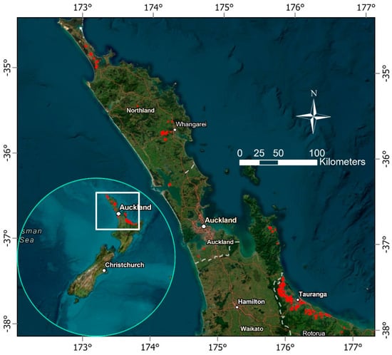
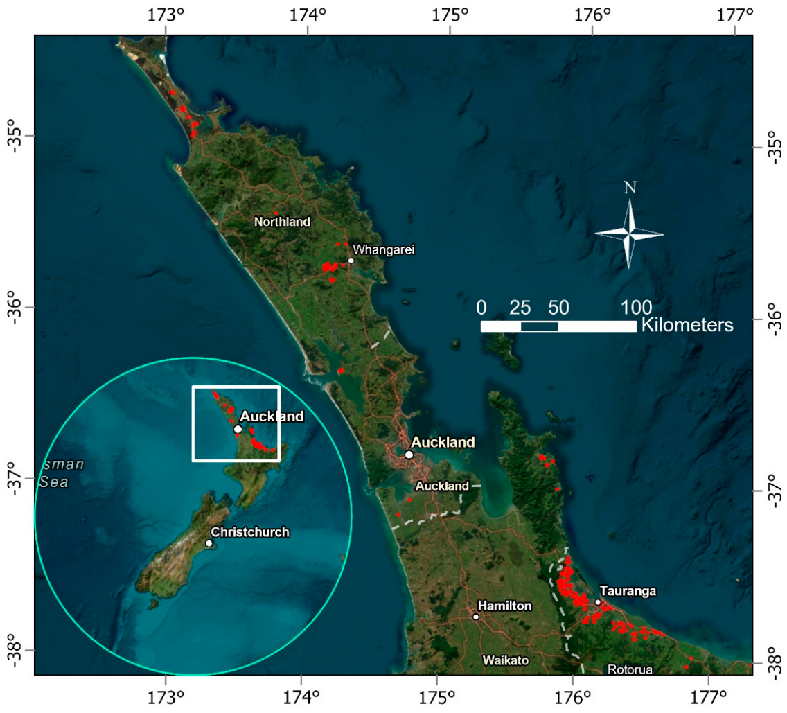
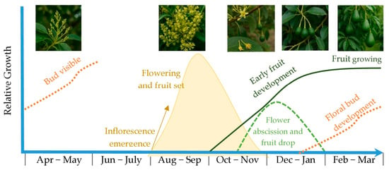
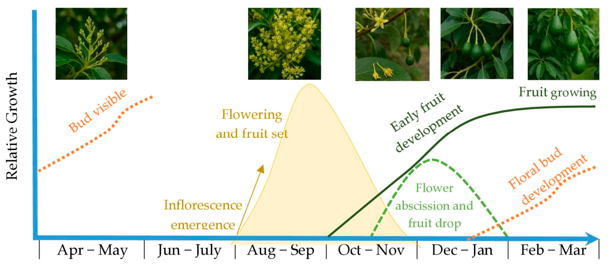
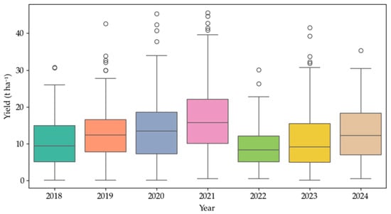
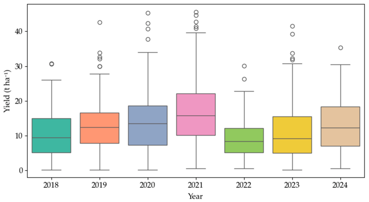
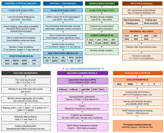
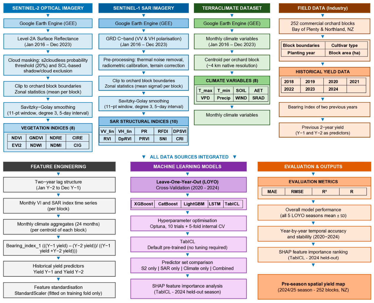
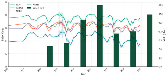
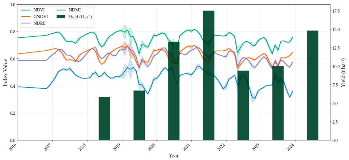
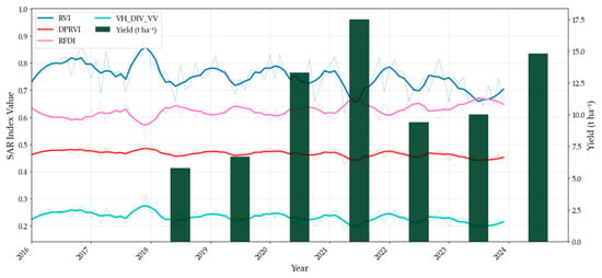
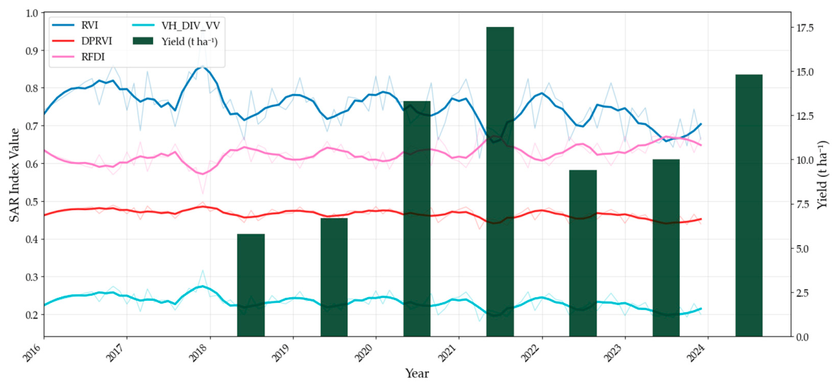
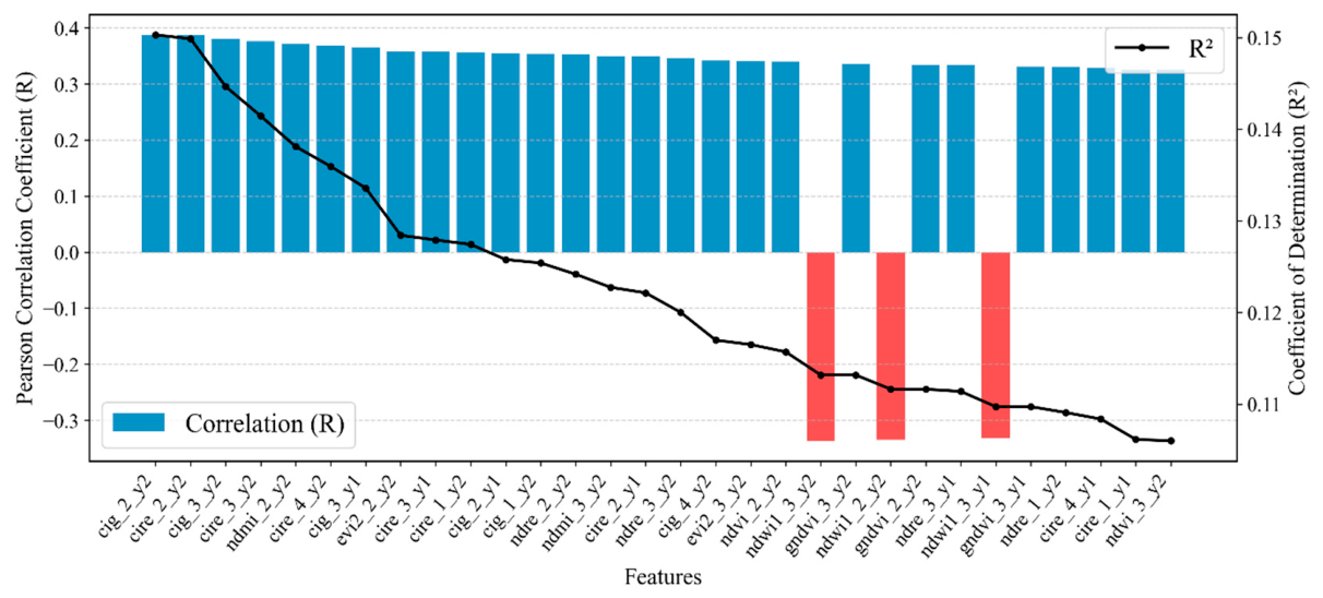
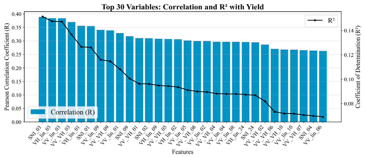
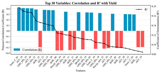
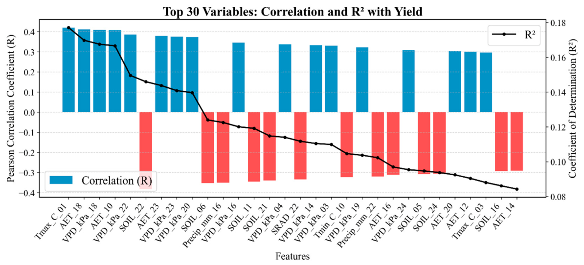
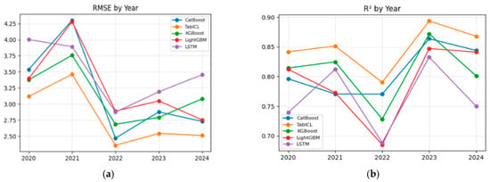
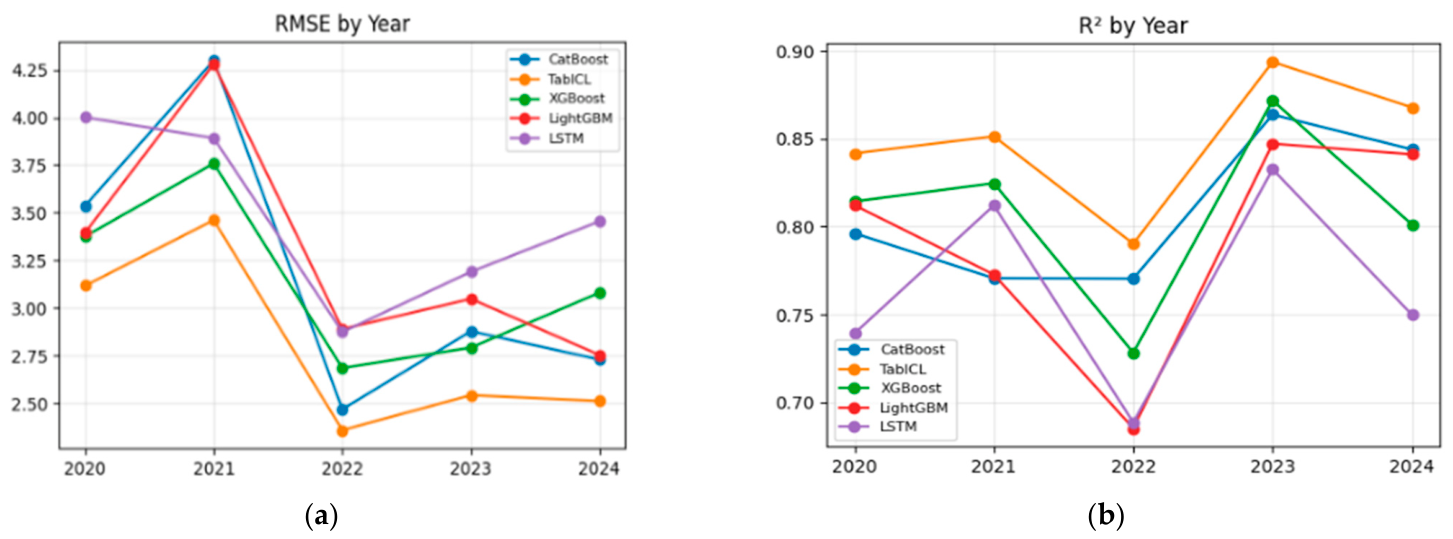
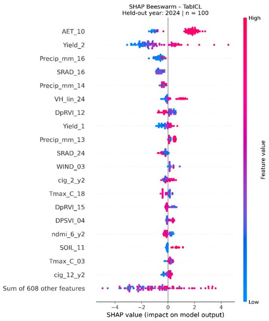
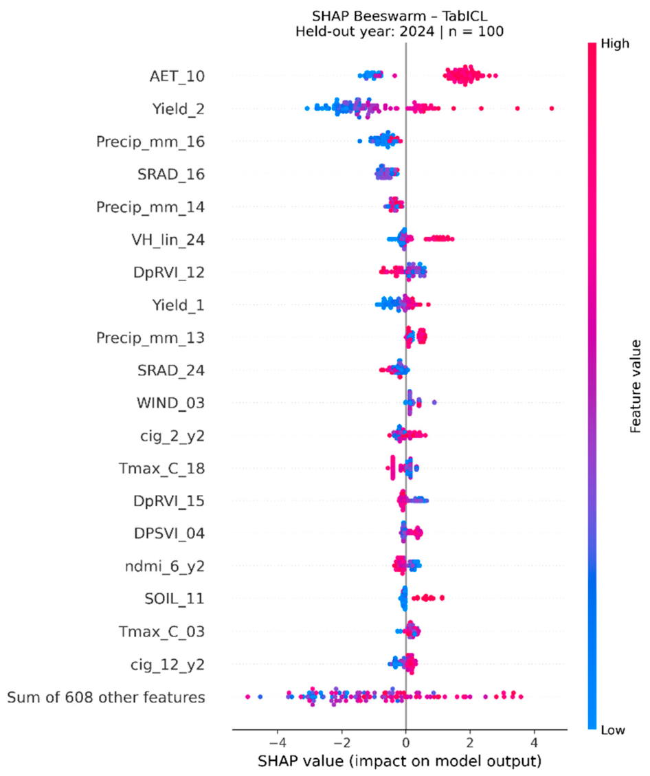
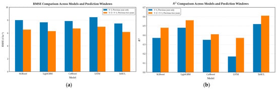
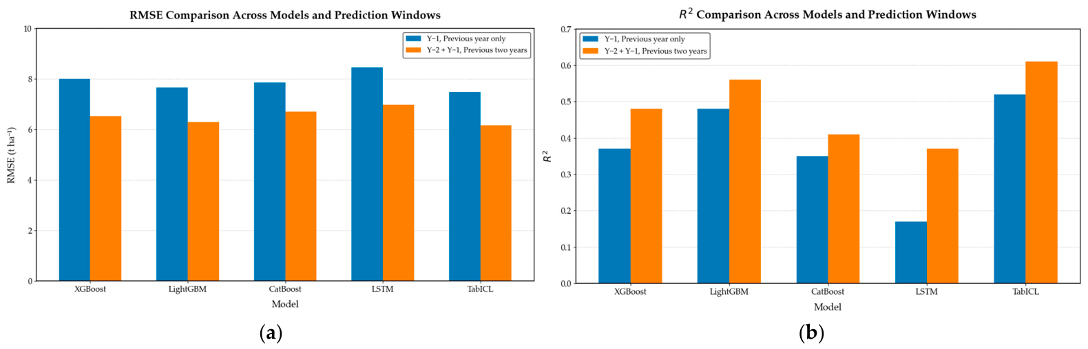
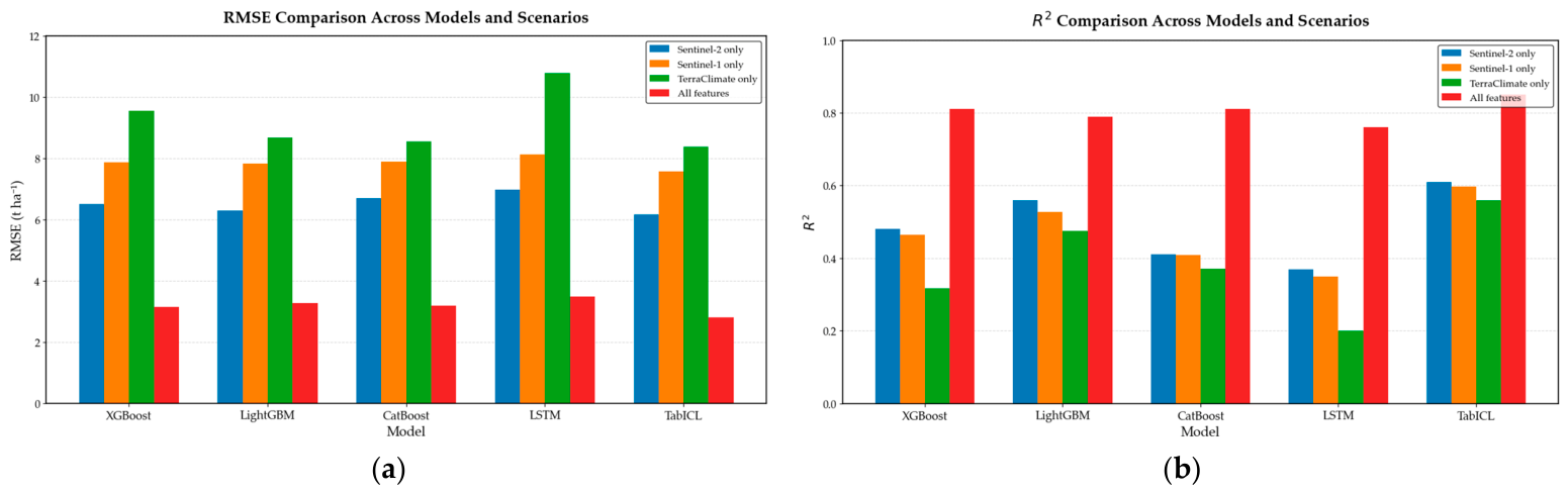
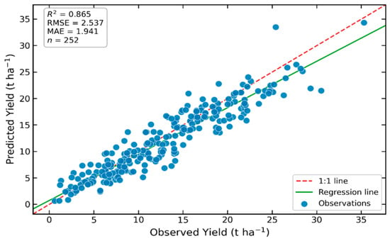
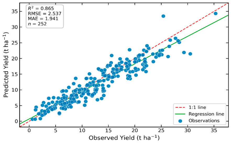
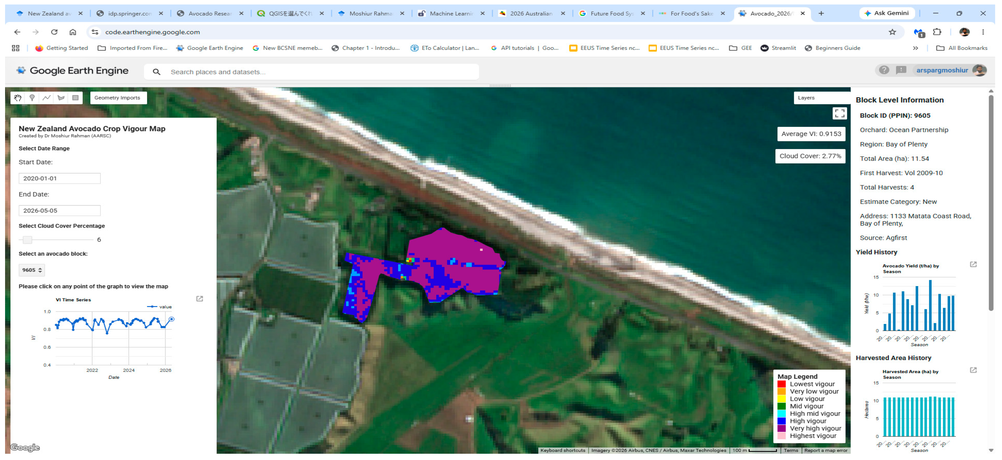

Disclaimer/Publisher’s Note: The statements, opinions and data contained in all publications are solely those of the individual author(s) and contributor(s) and not of MDPI and/or the editor(s). MDPI and/or the editor(s) disclaim responsibility for any injury to people or property resulting from any ideas, methods, instructions or products referred to in the content. |
© 2026 by the authors. Licensee MDPI, Basel, Switzerland. This article is an open access article distributed under the terms and conditions of the Creative Commons Attribution (CC BY) license.