Multi-Perspective Wildlife Monitoring with Drones and Camera Traps Using Deep Learning and Spatial Analysis

Highlights

What are the main findings?

• Spatial and spatiotemporal analyses showed broad correspondence between drone-derived wildlife distribution patterns and camera trap observations.
• Drone-based thermal imagery enhanced wildlife detectability, while paired RGB imagery provided landscape context.

What are the implications of the main findings?

• Drone and camera trap observations provide complementary spatial and temporal information for multi-perspective wildlife monitoring.
• Deep learning enables efficient wildlife detection from drone thermal and camera trap imagery, supporting cross-platform analysis.

Abstract

Wildlife monitoring is essential for biodiversity conservation, habitat management, and ecological assessment in protected landscapes. This study develops a multi-sensor, multi-perspective remote sensing approach that integrates drone-based thermal and RGB imagery, camera trap imagery, and deep learning models for wildlife monitoring in Chitwan National Park, Nepal. Thermal infrared drone imagery and daytime visible/nighttime infrared-illuminated camera trap images were organized into two independently constructed but related datasets for automated detection and cross-platform comparison. YOLOv8 and YOLOv11 models were trained and evaluated on the drone thermal dataset, while YOLOv5 and YOLOv11 models were trained and evaluated on the camera trap dataset. For cross-platform comparison, the analyses focused on deer and rhinos, the two taxa shared by both datasets. Detection outputs for these species were used to calculate drone-based detection densities and camera trap-based relative abundance index (RAI) values for spatial and spatiotemporal comparison. Among the evaluated models, YOLOv11s achieved the best performance on both datasets. In the drone dataset, YOLOv11s achieved an overall precision of 91.2%, recall of 85.4%, and mean Average Precision-50 (mAP50) of 93.6%. In the camera trap dataset, it achieved an overall precision of 95.5%, recall of 92.9%, and mAP50 of 95.4%. Spatial and spatiotemporal analyses showed broad correspondence between drone-derived wildlife distribution patterns and camera trap observations. These findings demonstrate that integrating aerial and ground-based sensing with deep learning can leverage the complementary advantages of each platform and enhance scalable wildlife monitoring across heterogeneous protected landscapes.

1. Introduction

Wildlife populations are fundamental components of ecosystem structure and function, and understanding their spatial distributions is essential for biodiversity conservation, habitat management, and ecological monitoring in protected landscapes [1,2,3]. Spatially explicit wildlife information can further reveal habitat-use patterns, identify areas of high species occurrence, and support assessments of ecosystem dynamics across space and time. However, wildlife monitoring remains challenging because animals are distributed across heterogeneous protected landscapes, where detection is affected by vegetation structure, illumination conditions, sensor perspective, and the limited spatial or temporal coverage of any single observation platform. Traditional field surveys are often labor-intensive, time-consuming, and limited in spatial and temporal coverage, with additional constraints related to observer bias and detection uncertainty [4]. These limitations highlight the need for scalable, spatially explicit monitoring approaches that can enhance wildlife detection, broaden observational coverage, and support landscape-scale ecological assessment.

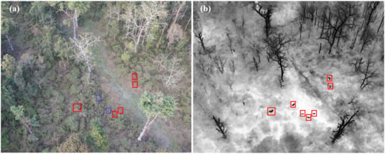
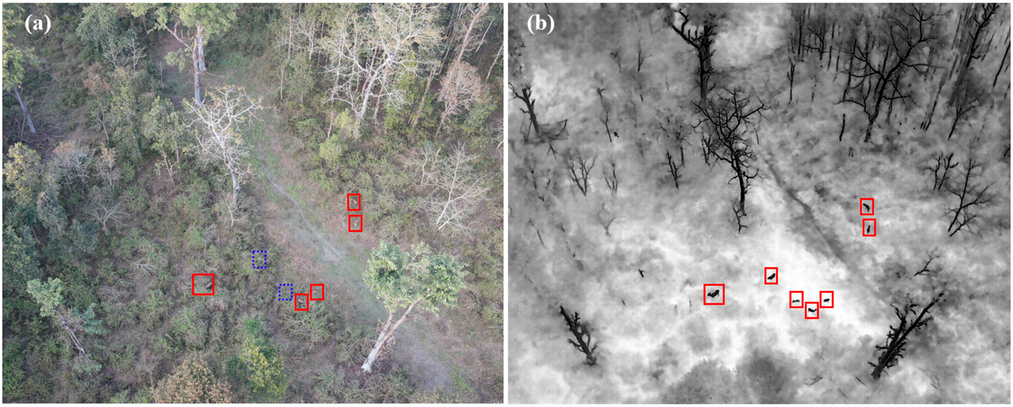
Recently, drones have emerged as a powerful tool for wildlife monitoring, offering broad spatial coverage and enabling access to remote or hard-to-access areas that are difficult to survey using traditional field survey methods [5,6]. Standard RGB sensors capture high-resolution true-color imagery, providing detailed visual information on habitat conditions, landscape context, and surface features that support wildlife monitoring and ecological interpretation. In addition to RGB imaging, thermal infrared sensors provide a specialized sensing capability by detecting differences in emitted radiation, often enabling animals to be distinguished from their surroundings based on surface temperature contrast [7]. Thermal sensors record infrared radiation emitted by surfaces, with the measured intensity primarily related to their apparent surface temperature and emissivity. As illustrated in Figure 1, the drone simultaneously acquired true color RGB and thermal infrared imagery. The paired images were collected at dusk on 10 February 2022, using a DJI Mavic 2 Enterprise Advanced. In the black-hot thermal palette, differences in apparent surface temperature between the deer and the surrounding vegetation and ground are represented as tonal contrast, with relatively warmer surfaces displayed in darker tones and cooler surfaces appearing lighter. Two deer are not visible in the RGB image but are clearly identifiable in the corresponding thermal image. Drones equipped with thermal sensors can improve wildlife detectability compared with standard visible-light systems, particularly under low-light conditions or in complex environments where animals are partially obscured by vegetation [8,9,10,11]. Recent research has further advanced drone-based wildlife monitoring through deep learning-based automated detection, improved detection of small targets in aerial imagery, RGB–thermal information fusion, and increasingly autonomous monitoring systems [12,13,14,15]. While drones extend spatial coverage, their observations are typically collected during discrete survey periods, creating a complementary role for ground-based monitoring systems that provide longer-term observations.

Figure 1. Paired drone imagery acquired at dusk on 10 February 2022, using a DJI Mavic 2 Enterprise Advanced, showing (a) true-color RGB imagery and (b) thermal infrared imagery. Two deer indicated by blue dashed boxes are difficult to distinguish in the RGB image but are more clearly identifiable in the corresponding thermal image.

Camera traps are static monitoring devices deployed at fixed locations, providing a ground-based and non-invasive approach for wildlife observation [16,17,18,19]. Typically equipped with RGB sensors and infrared illumination for nighttime imaging, camera traps are automatically triggered by animal movement within their detection range. They enable long-term monitoring while recording contextual information such as geographic location, timestamp, and ambient temperature, thereby supporting richer ecological analysis [20,21,22]. Overall, camera traps provide close-range observations from a horizontal ground-based perspective and can capture detailed animal appearances and activity patterns during both day and night. However, their spatial coverage is constrained by fixed placement, viewing direction, limited field of view, detection range, vegetation occlusion, and other obstructing landscape elements. In contrast, drones capture imagery from a vertical aerial perspective over broader areas and offer high mobility, with thermal sensors further improving animal detectability in complex environments. These differences highlight the contrasting spatial and temporal sampling characteristics of drones and camera traps.

Multi-sensor wildlife monitoring has shown strong potential in ecological research [23]. Early studies demonstrated the value of integrating multiple remote sensing sources for habitat analysis, combining passive optical imagery, including ETM+ and QuickBird, with active remote sensing data from LiDAR and SAR/InSAR to characterize forest structure for wildlife habitat assessment [24]. Subsequent multi-source data fusion approaches further integrated optical satellite imagery from platforms such as MODIS, Landsat, CBERS, and Terra with GPS tracking data to examine relationships between seasonal vegetation dynamics and wildlife movement patterns [25]. More recent studies have shifted toward ground-based and animal-borne sensing systems. For example, GPS tracking combined with RGB or thermal sensing has been used to capture fine-scale movement and behavioral patterns of wildlife [26,27]. Integrated multi-sensor platforms, such as BatRack, have also incorporated acoustic, visual, and environmental sensors to support multimodal ecological data collection [28]. These studies demonstrate the value of combining complementary sensing perspectives in ecological monitoring.

Despite rapid advances in drone-based sensing and automated wildlife detection, drones are still commonly investigated as an independent monitoring platform. In particular, relatively little attention has been given to how drone-based wildlife observations correspond spatially and spatiotemporally with long-duration observations from ground-based camera traps. The relationship between the broad, area-based perspective provided by drones and the temporally continuous, site-based perspective provided by camera traps therefore remains insufficiently examined. This gap limits our understanding of how the two monitoring perspectives provide complementary information on wildlife distribution across heterogeneous landscapes.

This study addresses this gap by integrating observations from drone-based thermal and RGB imagery with camera trap observations for multi-perspective wildlife distribution analysis. Cross-platform spatial and spatiotemporal comparison is the primary analytical focus of the study, while deep learning-based object detection serves as an enabling component for extracting wildlife observations from the two monitoring platforms. The purpose of this study is to examine how the spatial advantages of drone-based monitoring and the temporal advantages of camera traps provide complementary information on wildlife distribution patterns across heterogeneous landscapes. To achieve this, two independently annotated datasets were constructed from drone thermal imagery and camera trap imagery, and deep learning-based object detection models were trained and evaluated separately for each dataset. The resulting detections were used to calculate drone-based detection densities and camera trap-based relative abundance index (RAI) values, which were standardized for cross-platform comparison. The aerial and ground-based wildlife distributions were then compared through spatial and spatiotemporal analyses to examine correspondence between the two monitoring perspectives at different spatial and temporal scales.

The main contributions of this research are threefold. First, we develop a multi-perspective wildlife monitoring approach that integrates drone thermal, drone RGB, and camera trap observations to examine wildlife distributions from complementary aerial and ground-based perspectives. Second, we standardize platform-specific wildlife observations using drone-derived detection density and camera trap-derived RAI, enabling spatial comparison between monitoring platforms with fundamentally different sampling designs. Third, we conduct cross-platform spatial and spatiotemporal analyses to examine correspondence and differences in wildlife distribution patterns across heterogeneous protected landscapes.

2. Methods

2.1. Study Area

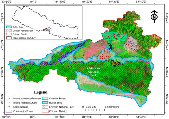
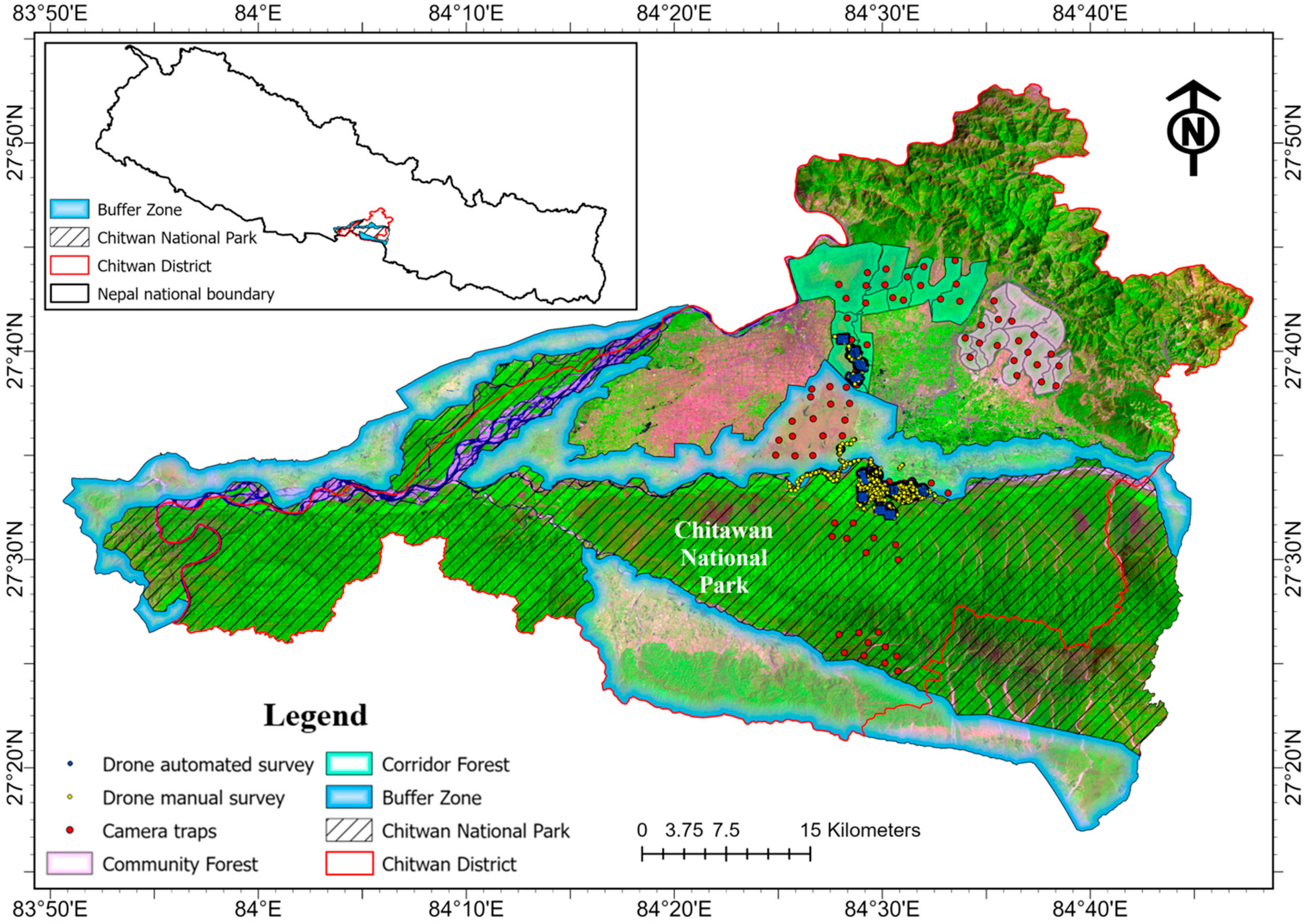
The study area encompasses Chitwan National Park (CNP) in south-central Nepal and its surrounding heterogeneous landscape (Figure 2). CNP covers approximately 932 km² and is a UNESCO World Heritage Site recognized for its exceptional biodiversity [29]. The park supports a wide range of wildlife species, including the endangered rhinos (One Horned Rhinoceros; Rhinoceros unicornis), tigers (Royal Bengal Tiger; Panthera tigris tigris), Asian elephants, multiple deer species, primates, and more than 500 bird species [30]. The region has a tropical monsoon climate, with a hot dry season from March to early June, followed by a monsoon period from late June to September during which most annual precipitation occurs.

Figure 2. Chitwan National Park and its surrounding landscapes. False color image of Landsat 8 collected on 5 April 2022. Red: band 6, 1560–1660 nm; Green: band 5, 845–885 nm; Blue: band 4, 630–680 nm.

The study area includes four major landscape units: Chitwan National Park, Buffer Zone, Corridor Forest, and Community Forest. Surrounding CNP is a Buffer Zone of approximately 750 km² characterized by a mixed-use landscape of forests, agricultural land, and settlements, supporting a substantial local population [31,32]. As a conservation-oriented transition area between the park and human-dominated landscapes, the Buffer Zone allows regulated local resource use while also serving as an important interface where human–wildlife interactions frequently occur. North of the Buffer Zone lies the Corridor Forest, which provides important habitat connectivity and supports wildlife movement between lowland and higher-elevation areas [33]. Community Forests in Nepal are locally managed forest areas handed over to Community Forest User Groups, which are legally authorized to protect, manage, and use forest resources under approved management plans [34]. Unlike strictly protected park areas, Community Forests combine conservation with regulated local resource use, allowing communities to collect forest products while participating directly in forest governance and restoration. CNP was selected because, together with its Buffer Zone, Corridor Forest, and Community Forest, it forms a connected landscape with contrasting ecological and land-use conditions while supporting conservation-priority wildlife, making it suitable for evaluating complementary drone and camera trap monitoring.

2.2. Dataset Construction

2.2.1. Drone Thermal Dataset

Drone imagery was collected across the study area between February and July 2022, primarily during the early morning (05:30–08:30) or evening (17:00–19:00), depending on suitable weather and field conditions for best temperature contrast between wildlife animals and their ambient background. Before each flight, standard calibration and pre-flight system checks were performed, including checks of the camera, gimbal, and positioning status. Data were collected using a DJI Mavic 2 Enterprise Advanced (SZ DJI Technology Co., Ltd., Shenzhen, China) platform equipped with both thermal infrared and RGB sensors. The system simultaneously acquired thermal infrared imagery at a resolution of 640 × 512 pixels and high-resolution true-color RGB imagery at 8000 × 6000 pixels. Thermal imagery was used as the primary data source for wildlife detection, while corresponding RGB imagery was used for visual interpretation and verification.

Data acquisition followed two drone survey strategies (Figure 2). During manual surveys, the drone was actively controlled by a pilot to locate wildlife and acquire targeted thermal images. Manual flights followed a pilot-controlled pattern at a standard altitude of 80 m above ground level (AGL) and a speed of approximately 3 m/s. Oblique views were used for navigation and visual identification, whereas images of detected wildlife were captured at nadir. When vegetation obstructed definitive species identification, the drone was lowered to approximately 40 m AGL to obtain clearer images. During automated surveys, the drone followed pre-defined flight paths over rectangular survey regions to systematically collect imagery. Automated flight missions were planned using the Mission Flight function in the DJI Pilot app (version 2.5). The missions were conducted at 80 m AGL and a flight speed of 3 m/s, with 80% forward and side overlapping. The gimbal was set for nadir image acquisition, and images were captured sequentially at distance-based intervals. Thermal images acquired from manual surveys were used to construct the training, validation, and testing dataset, whereas imagery collected from automated surveys was used for large-area wildlife detection. The resulting detections were then analyzed to characterize spatial distribution patterns across the study area.

A total of 28,053 images were collected from the two survey modes. All images acquired from manual surveys contained wildlife, whereas only a subset of images from automated surveys included wildlife detections. The open-access platform ImageLab was used to annotate wildlife in the thermal images. The annotations were reviewed by two wildlife researchers experienced in identifying large mammals in CNP, and the final species labels were verified by the field drone pilot.

The dataset was randomly partitioned into training, validation, and test sets using a 70:15:15 split for deep learning model development and evaluation. After dataset partitioning, image rotation and mosaic augmentation were applied to the underrepresented buffalo and rhino classes in the training subset to reduce class imbalance; no augmented images were included in the validation or test subsets. In addition, to standardize thermal images collected with different color palettes, all thermal imagery was converted to a black-hot palette, in which warmer objects appear darker and cooler objects appear lighter. No other image corrections were applied to the drone thermal images. Although additional wildlife species were observed during the drone surveys, their limited numbers were insufficient for constructing representative detection classes; therefore, the curated dataset focused on buffalo, rhino, and deer. The image and instance statistics of the drone thermal dataset are summarized in Table 1. Buffalo was included in the drone thermal dataset for detector training and evaluation but was excluded from the cross-platform analyses because it was not a target class in the camera trap dataset. Therefore, only deer and rhinos were used for the multi-perspective comparison.

Table 1. Image and instance statistics of the drone thermal dataset.

Class	Buffalo	Rhino	Deer
Images	2277	2277	2277
Instances	11,140	12,094	13,509

2.2.2. Camera Trap Dataset

Camera trap images were collected using Bushnell Core DS-4K (Bushnell Outdoor Products, Overland Park, KS, USA) cameras configured for motion-triggered image capture, with 32-megapixel still images recorded when movement was detected. Camera traps were strategically deployed at locations with a high likelihood of wildlife activity, and the GPS coordinates of each station were recorded prior to installation. A total of 80 cameras were installed across the study area, including 20 in CNP, 20 in the Buffer Zone, 20 in the Corridor Forest, and 20 in the Community Forest. All camera traps were serviced by trained field staff, and the stored data were retrieved approximately every two months.

The resulting imagery captured a diverse set of wildlife species, domestic animals, and humans. The image and instance statistics of the camera trap dataset are summarized in Table 2. Image annotation was conducted using the Roboflow platform [35]. Using Roboflow, the annotated images were randomly partitioned at the image level into training, validation, and test subsets in proportions of 70%, 20%, and 10%, respectively. The different ratios compared with the drone thermal dataset reflect differences in dataset scale and class structure: the smaller three-class drone dataset used equal validation and test proportions, whereas the larger eight-class camera trap dataset allocated a larger validation subset for multi-class model selection while retaining sufficient test images for final evaluation. To reduce class imbalance while preventing data leakage, random rotation augmentation was applied to the underrepresented tiger, rhino, and elephant classes exclusively within the training subset; no augmented images were included in the validation or test subsets. All images were resized to 640 × 640 pixels, a commonly used input size for the You Only Look Once (YOLO)-based object detection [36], to standardize model input, reduce computational cost, and accelerate training. Because animals in camera-trap images were generally captured at close range and occupied a substantial portion of the images, the resized images retained sufficient detail for detection. No additional denoising, infrared exposure correction, or motion-blur correction was applied.

Table 2. Image and instance statistics of the camera trap dataset.

Class	Tiger	Rhino	Elephant	Sambar Deer	Spotted Deer	Rhesus Macaques	Human	Domestic Goat
Images	1211	2733	1776	3639	2145	2220	1842	1120
Instances	1211	2805	1884	3931	4996	2997	2081	3042

2.3. Deep Learning Models

In this study, the YOLO family of real-time object detection models was adopted for automated wildlife detection. These models are widely used in ecological monitoring due to their efficiency and strong performance in detecting objects in complex environments [37].

Among the YOLO models, YOLOv5 is a widely applied model known for its balance between detection accuracy and computational efficiency. YOLOv5 adopts an anchor-based detection framework, in which predefined anchor boxes are used as initial references for object localization [38]. YOLOv8 introduces an anchor-free detection paradigm that directly predicts object locations from feature maps, reducing dependence on predefined anchors and simplifying model training [39]. YOLOv11 was selected as a recent YOLO architecture available when the model experiments were conducted. Compared with YOLOv8, YOLOv11 replaces the C2f modules with more computationally efficient C3k2 blocks and introduces a C2PSA attention module after the spatial pyramid pooling layer to strengthen spatial feature representation. Its neck also incorporates C3k2 blocks to improve multi-scale feature fusion and detection robustness [40].

Each YOLO version provides multiple model variants, including nano (n), small (s), medium (m), large (l), and extra-large (x), which vary in network depth and width, leading to differences in computational cost and detection performance. In this study, different model configurations were evaluated for the two datasets. For the drone thermal dataset, eight models were trained and evaluated, including YOLOv8n, YOLOv8s, YOLOv8m, YOLOv8l, YOLOv11n, YOLOv11s, YOLOv11m, and YOLOv11l, to compare the performance of different anchor-free YOLO architectures on thermal imagery. For the camera trap dataset, six models were trained and evaluated, including YOLOv5n, YOLOv5s, YOLOv5m, YOLOv11n, YOLOv11s, and YOLOv11m, enabling comparison between the anchor-based YOLOv5 architecture and the anchor-free YOLOv11 architecture.

All models were initialized with their respective official pretrained weights and then fine-tuned on the corresponding training subsets using a batch size of 32 for a maximum of 150 epochs on an NVIDIA RTX 3090 GPU with 24 GB of memory. All model fine-tuning, evaluation, and inference were performed offline on this workstation after image acquisition; no model inference was conducted onboard the drone or camera traps. The Stochastic Gradient Descent (SGD) optimizer was used with an initial learning rate of 0.01 and a weight decay of 0.0005. Early stopping was configured with a patience of 100 epochs. A random seed of 0 was used, and deterministic training was enabled to improve reproducibility. For YOLOv5, the default anchor configuration associated with the pretrained model was retained, whereas YOLOv8 and YOLOv11 use anchor-free detection heads. The same training settings were maintained across the evaluated model configurations to support a consistent comparison, rather than independently optimizing hyperparameters for each architecture. The best-performing model for each dataset was selected based on standard evaluation metrics (described below) and subsequently used for wildlife detection. The model comparison was intended to select a reliable detector for the subsequent multi-perspective analysis.

2.4. Evaluation Metrics

To evaluate the performance and reliability of the object-detection models, four standard metrics were used: precision, recall, mean Average Precision (mAP) at an Intersection over Union (IoU) threshold of 0.50 (mAP50), and mAP averaged over IoU thresholds from 0.50 to 0.95 (mAP50–95). During training, model performance was monitored on the validation set, and the checkpoint with the best validation performance was retained for each model configuration. Final performance was evaluated on the respective fully annotated held-out test sets, which were not used for model training or checkpoint selection. Model predictions on each held-out test set were compared with the corresponding ground-truth bounding-box and class annotations to determine true positives, false positives, and false negatives and calculate the four evaluation metrics. The same standard YOLO evaluation procedure was applied across all model configurations to support consistent comparisons. Precision and recall were defined as:

$$Precision= {\displaystyle \frac{TP}{TP+FP}}$$

(1)

$$Recall={\displaystyle \frac{TP}{TP+FN}}$$

(2)

where TP, FP, and FN denote true positives, false positives, and false negatives, respectively. Precision measures the proportion of predicted detections that are correct, whereas recall measures the proportion of ground-truth objects that are successfully detected.

The mAP50 metric evaluates detection performance at a fixed IoU threshold of 0.50, reflecting the model’s ability to correctly identify objects with moderate localization accuracy. In contrast, mAP50–95 provides a more stringent evaluation by averaging mAP across multiple IoU thresholds from 0.50 to 0.95 in increments of 0.05, requiring increasingly precise overlap between predicted and ground-truth bounding boxes. As a result, mAP50–95 provides a more comprehensive assessment of object detection performance than mAP50, as it evaluates both detection accuracy and localization precision across multiple IoU thresholds.

To assess the potential influence of class imbalance in the camera trap dataset, class-specific detection metrics and normalized confusion matrices were examined in addition to the overall evaluation metrics.

2.5. Multi-Perspective Comparison

The multi-perspective comparison focused on species shared by both datasets. Deer and rhinos were selected because they were detected in both drone and camera trap imagery. To harmonize labels across platforms, detected spotted deer and sambar deer in the camera trap data were aggregated into a single deer class.

Detection outputs from the best-performing deep learning models were converted into georeferenced point data using the geographic coordinates associated with the drone flight locations and camera trap sites. These points were then used to examine species-specific distribution patterns and compare wildlife monitoring results from aerial and ground-based perspectives.

2.5.1. Standardization of Detections

Standardization was conducted to account for differences in the sampling geometry and duration of the two monitoring platforms. Drone-based detections were generated from area-based surveys over a footprint at a specific point in time, whereas camera trap detections were recorded at fixed point locations over a duration of time. To support cross-platform comparison, the detection outputs from both platforms were transformed into spatially comparable indicators before subsequent analysis.

Drone surveys were conducted in ten regions. For each region, drone-based observation density was calculated by dividing the total number of detections of a species within the region by its corresponding area. Each drone survey region was then represented by its centroid, and the corresponding region-level observation density was assigned to that centroid for subsequent spatial comparison with camera trap observations.

Camera trap observations were summarized using the species-specific RAI for each camera trap, which was calculated as the number of independent detections of a species divided by the total number of camera trap days and multiplied by 100 [41]. RAI serves as a time-standardized measure of detection frequency across camera trap sites. Because drone-derived detection density and camera trap-derived RAI have different units and value ranges, the two measures were independently normalized to a range of 0–1 using min–max normalization for each species before cross-platform comparison.

2.5.2. Spatial Analysis

To enable direct comparison between drone and camera trap observations, the normalized RAI values from camera trap sites were spatially interpolated to the centroid of each drone survey region. Inverse distance weighting (IDW) algorithm was used to perform the interpolation, based on the assumption that spatial similarity decreases with distance [42,43]. For the centroid of each drone survey region, the estimated normalized RAI was calculated from those of nearby camera trap sites, with closer sites contributing more to the interpolated value. The resulting IDW-interpolated normalized RAI values were then compared with the normalized drone-derived observation densities at the corresponding region centroids. This procedure allowed camera trap observations to be spatially aligned with those of drone survey regions, thereby supporting cross-platform comparison of wildlife distribution patterns.

To further examine the contrasting deer patterns between selected regions, within-image deer aggregation was calculated as the mean number of deer detections per deer-positive image, calculated by dividing the total number of deer detections by the number of images containing at least one deer.

2.5.3. Spatiotemporal Analysis

To evaluate cross-platform consistency over a shared period of time, kernel density estimation (KDE) was applied to visualize the spatial distribution patterns of wildlife detections from drone imagery and camera trap observations. KDE converts discrete detection points into continuous density surfaces, where areas with higher concentrations of detections correspond to higher density values, and density decreases with distance from detection concentrations [44,45]. While the normalized drone-derived observation densities and IDW-interpolated normalized RAI values were used for quantitative cross-platform comparison, KDE provided continuous density surfaces for visualizing and comparing relative spatial patterns of wildlife activity between the two platforms.

The KDE-based spatiotemporal analysis focused on May 2022, a period of high detection activity for both deer and rhinos in the study area. Drone-based detections and camera trap observations from this period were used to generate platform-specific density surfaces, allowing for visual comparison of relative wildlife distribution patterns across aerial and ground-based perspectives.

To further examine fine-scale spatiotemporal correspondence, a one-day case study was conducted on 26 May 2022, in the Buffer Zone. Deep learning-based detections from drone thermal imagery and camera trap imagery acquired within a one-hour interval were compared to evaluate whether both platforms recorded rhino activity within close temporal and spatial proximity. Paired drone RGB imagery was also examined to provide additional landscape context for the drone-based thermal detection. This case-study analysis narrowed the comparison from monthly activity patterns to same-day observations, providing a more direct assessment of cross-platform consistency between aerial and ground-based wildlife monitoring.

3. Results

3.1. Drone-Based Wildlife Detection

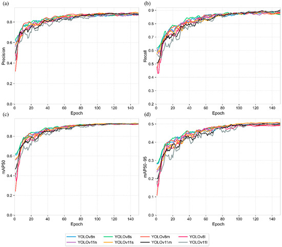
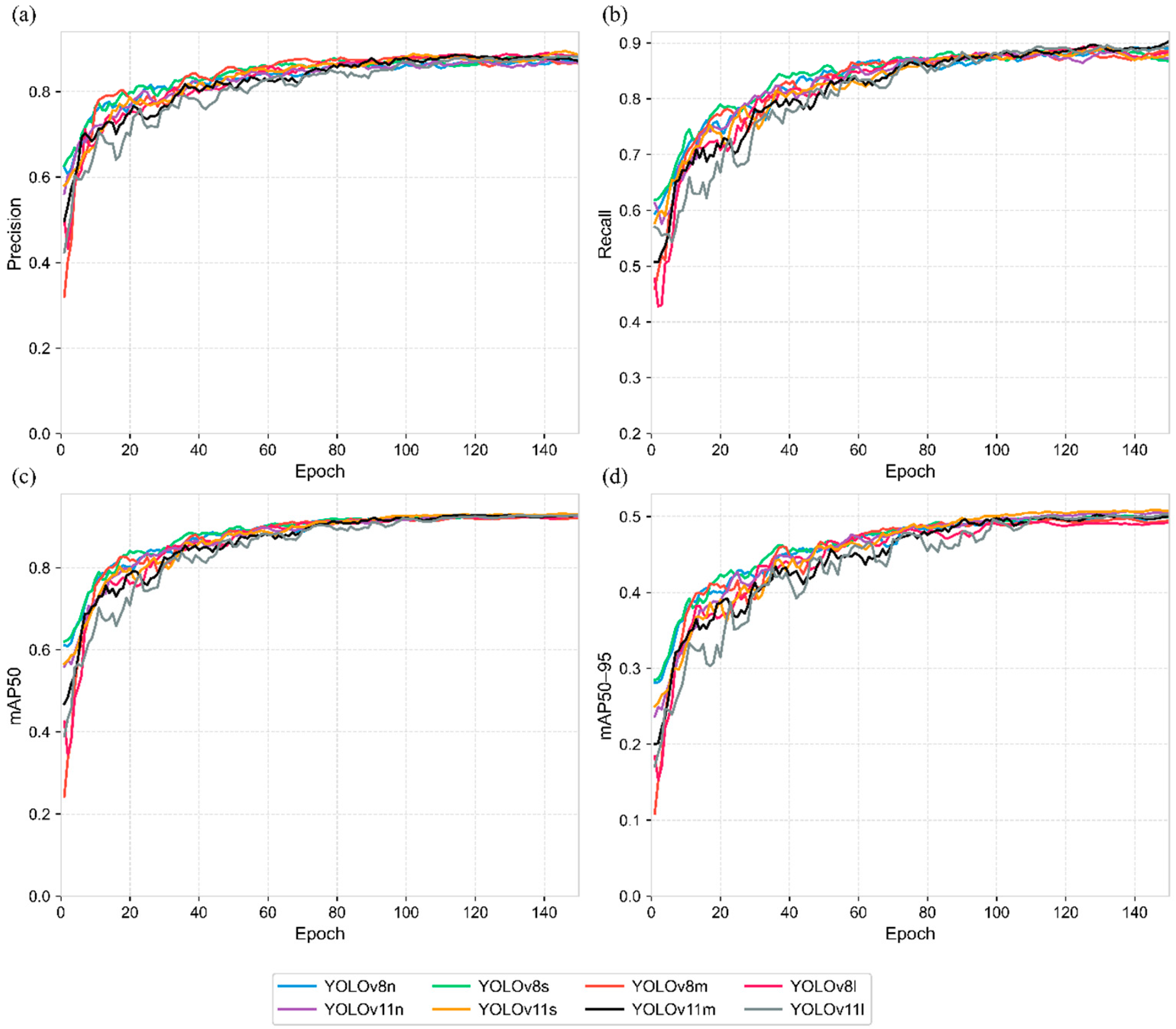
The validation performance curves of the evaluated YOLO models are shown in Figure 3. Performance improved rapidly during the initial training phase, particularly within the first 20–30 epochs, and then gradually stabilized. As training progressed, the curves became more stable, indicating effective convergence. After approximately 100 epochs, mAP50 had largely plateaued, while precision, recall, and mAP50–95 showed minor further improvements. Among the evaluated models, YOLOv11s achieved the strongest overall validation performance, particularly for precision, mAP50, and mAP50–95, suggesting robust detection and localization capability for wildlife detection in drone thermal imagery.

Figure 3. Validation performance curves of the evaluated YOLO models over 150 training epochs: (a) precision, (b) recall, (c) mAP50, and (d) mAP50–95. The curves were smoothed using a centered five-epoch moving average for visualization only. Model selection and the reported performance metrics were based on the original unsmoothed values.

Table 3 presents the testing performance of YOLOv8 and YOLOv11 models on the drone thermal dataset across accuracy and efficiency metrics. YOLOv11 variants outperformed YOLOv8 models across most metrics, indicating that improvements in feature representation and multi-scale prediction contribute to more robust detection and localization performance in thermal imagery. Among all models, YOLOv11s achieved the best overall performance, with the highest precision (0.912), mAP50 (0.936), and mAP50–95 (0.499). Although YOLOv11m and YOLOv11l have larger model capacities and more parameters, they do not outperform YOLOv11s on the drone thermal dataset. This is likely because thermal imagery has much lower spatial resolution than the RGB imagery, causing wildlife targets to appear as small, localized heat signatures with limited texture information. Larger and deeper models, such as YOLOv11m and YOLOv11l, involve more hierarchical feature extraction and down-sampling, which may reduce sensitivity to fine-scale spatial signals and weaken localization performance. In contrast, YOLOv11s provided sufficient representational capacity while better preserving small-target information, resulting in stronger performance on drone thermal imagery.

Table 3. Comparison of testing performance metrics for drone thermal dataset.

Models	Precision	Recall	mAP50	mAP50–95	Inference (ms)	FPS	Parameters (Million)
YOLOv8n	0.877	0.831	0.901	0.475	2.6	384.6	3.01
YOLOv8s	0.865	0.860	0.910	0.484	3.9	256.4	11.13
YOLOv8m	0.828	0.869	0.901	0.477	5.0	200.0	25.84
YOLOv8l	0.888	0.836	0.908	0.479	7.5	133.3	43.61
YOLOv11n	0.866	0.832	0.914	0.484	2.7	370.4	2.58
YOLOv11s	0.912	0.854	0.936	0.499	3.6	277.8	9.41
YOLOv11m	0.887	0.858	0.906	0.484	5.1	196.1	20.03
YOLOv11l	0.858	0.855	0.910	0.481	6.2	161.3	25.28

In terms of efficiency, lightweight models such as YOLOv8n and YOLOv11n achieved the fastest inference speeds and smallest parameter sizes, whereas larger models incurred higher computational costs. Overall, YOLOv11s provided the best trade-off between detection accuracy and computational efficiency for wildlife detection in drone thermal imagery, achieving an inference rate of 277.8 Frames Per Second (FPS) on the RTX 3090 GPU. The reported FPS values reflected GPU-based inference performance under the experimental computing environment rather than onboard drone processing. In this study, drone imagery was processed offline after data acquisition.

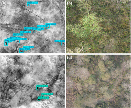
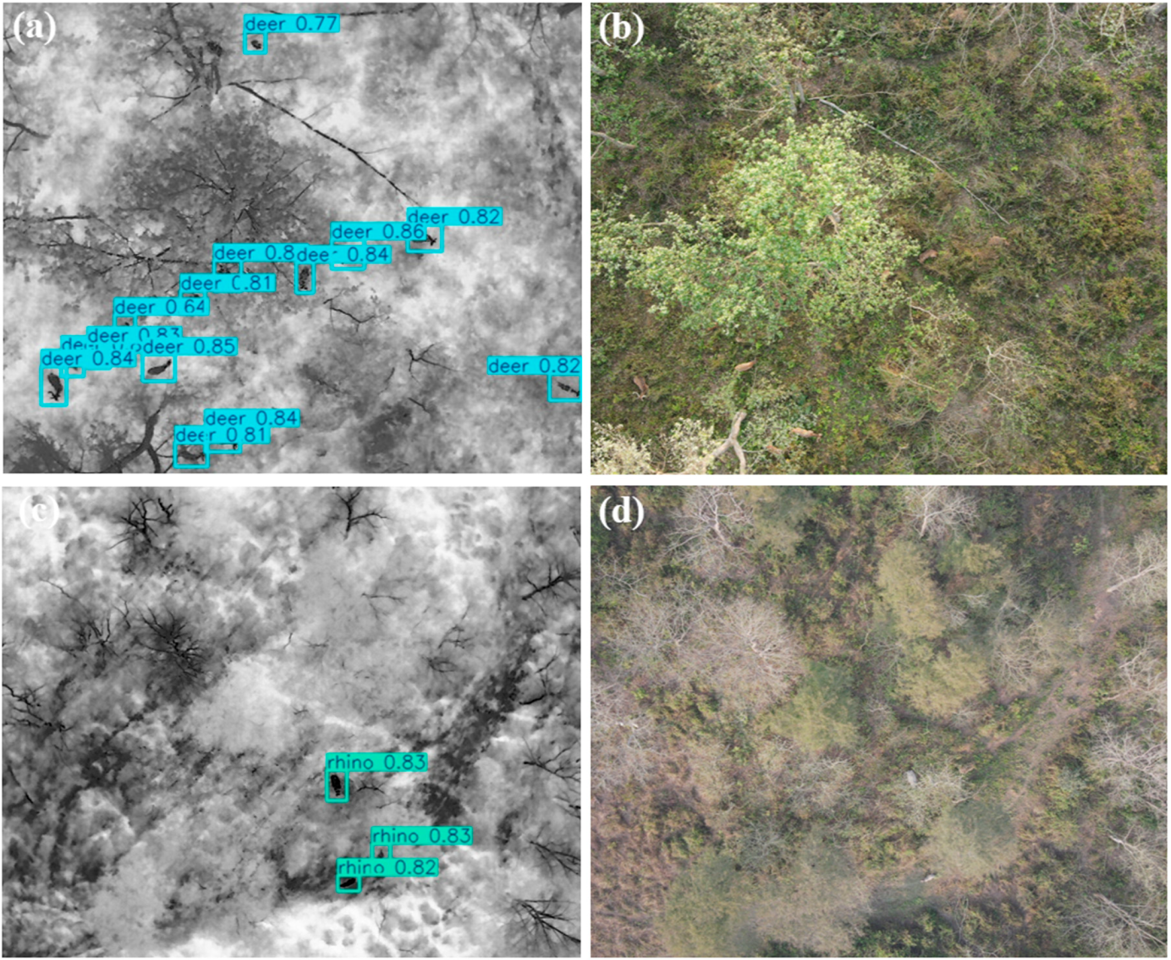
The best-performing YOLOv11s model, using the weights from its best-validation checkpoint, was therefore applied to detect wildlife in the drone automated survey areas. Figure 4 shows representative detection results from drone thermal imagery, with corresponding RGB imagery provided as visual reference. In Figure 4a, 14 deer were identified in the thermal image, six of which were not visible in the RGB image (Figure 4b) due to canopy occlusion. A similar pattern was observed in Figure 4c, where three rhinos were detected in the thermal image, one of which was not visible in the corresponding RGB image (Figure 4d). These examples demonstrated that thermal drone imagery can improve the detection of wildlife obscured by canopy cover in RGB imagery, while further highlighting the effectiveness of YOLOv11s for automated wildlife detection in complex forested environments.

Figure 4. Representative wildlife detection results of the YOLOv11s model on drone thermal imagery, with corresponding RGB images for visual reference: (a,c) thermal images showing detected deer and rhinos and (b,d) corresponding RGB images of the same scenes.

3.2. Camera Trap-Based Wildlife Detection

YOLO models trained on the camera trap dataset were comprehensively evaluated in our previous study [38]. Compared with YOLOv5 models, YOLOv11 models achieved substantially faster inference speeds while maintaining strong detection accuracy. Considering both accuracy and efficiency, YOLOv11s was selected as the most suitable model for object detection from camera trap imagery. For the selected YOLOv11s model, class-specific test results showed strong detection performance across classes with different sample frequencies, including the less frequent tiger, elephant, and rhino classes (Table S1). Normalized confusion matrices for the evaluated camera trap models further showed limited inter-class confusion (Figure S1).

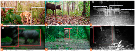
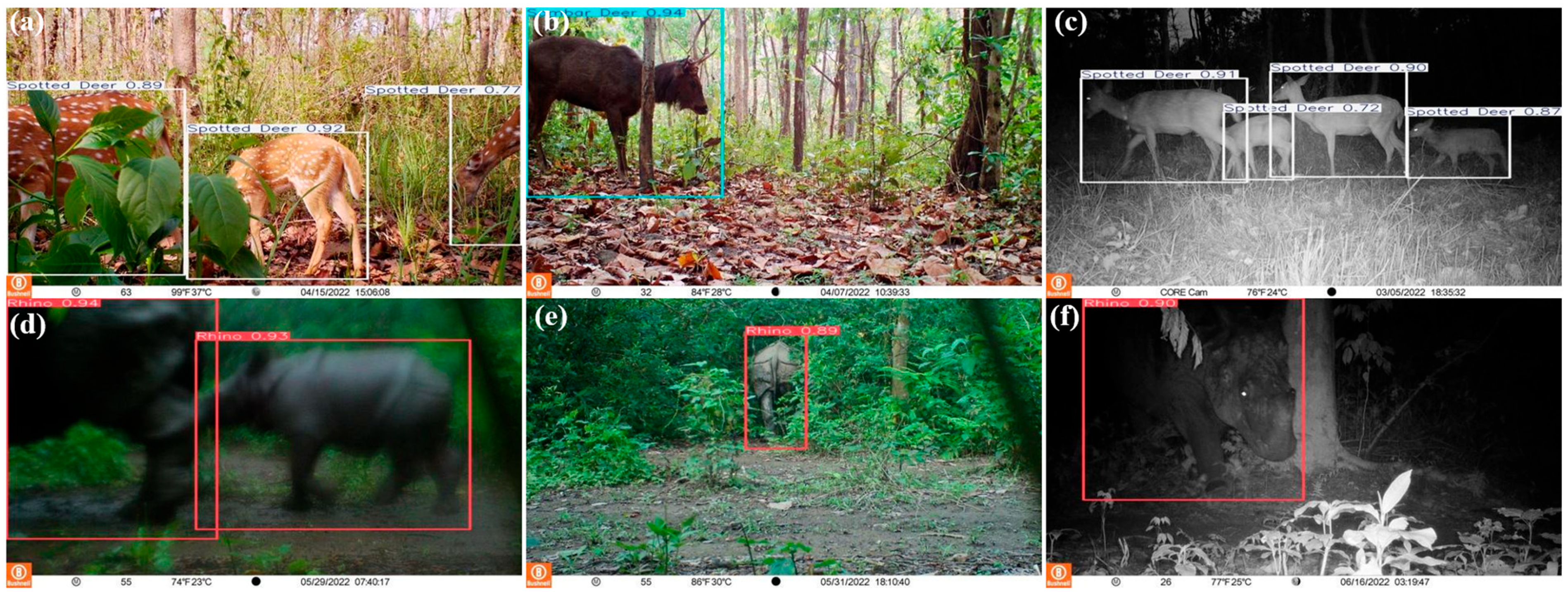
The best-performing YOLOv11s model was applied to 57,037 camera trap images acquired across the study area between February and July 2022. Deer detections, including spotted deer and sambar deer, and rhino detections were extracted to match the class of the drone thermal dataset and support multi-perspective monitoring. Representative detection results are shown in Figure 5. The model successfully detected animals under challenging conditions, including occlusion by vegetation (Figure 5a) and a tree trunk (Figure 5b), overlapping individuals (Figure 5c), motion blur (Figure 5d), partial visibility (Figure 5e), and nighttime infrared-illuminated scenes with limited visual detail (Figure 5f). These results demonstrate that YOLOv11s can support automated, high-throughput wildlife detection in camera trap imagery, providing reliable detection outputs for subsequent spatial analysis.

Figure 5. Representative detection results of the YOLOv11s model on the camera trap dataset under challenging conditions: (a) occlusion by vegetation; (b) tree-trunk obstruction; (c) overlapping individuals; (d) motion blur; (e) partial visibility; and (f) limited visual detail.

3.3. Multi-Perspective Monitoring Analysis

3.3.1. Platform-Specific Spatial Patterns

As shown in Table 4, drone-based detections revealed distinct spatial patterns for deer and rhinos. Deer were detected across all regions but exhibited a heterogeneous spatial distribution. The highest deer densities were observed in Corridor Forest, particularly in Region 4 (550.28 km⁻²) and Region 3 (189.41 km⁻²). Regions 8 (in CNP) and 1 (in Corridor Forest), however, showed the lowest deer densities at 19.18 km⁻² and 28.08 km⁻², respectively.

Table 4. Drone-derived wildlife detection counts and densities.

Region	Area (km2)	Deer		Rhino
		Count	Density (km−2)	Count	Density (km−2)
1	0.46	13	28.08	0	0.00
2	0.44	23	52.87	11	25.29
3	0.49	93	189.41	2	4.07
4	0.36	197	550.28	0	0.00
5	0.34	54	158.36	9	26.39
6	0.39	24	61.07	18	45.80
7	0.36	66	183.84	1	2.79
8	0.42	8	19.18	1	2.40
9	0.38	47	125.00	2	5.32
10	0.37	26	69.89	2	5.38

Unlike deer, rhino occurrences were clustered in particular areas rather than spread across all the regions. The highest rhino density was observed in the Buffer Zone in Region 6 (45.80 km⁻²). The next highest concentrations of rhinos were found in Region 5 inside CNP (26.39 km⁻²) and Region 2 in the Corridor Forest (25.29 km⁻²). In other regions, rhinos were either absent or detected at low densities, with no more than two detections recorded per region.

Camera trap observations showed substantial spatial variation in deer detection frequency and RAI among the sites located near the drone survey regions, as shown in Table 5. Deer were detected at all nearby camera trap sites, but their detection frequency varied substantially across locations. The RAI values indicated the highest deer detection activity at CRF05, with an RAI of 5600.68, followed by CRF02 and BZF17, with RAI values of 3820.55 and 1952.34, respectively. In contrast, lower deer activity was observed at BZF19 and CRF04, with RAI values of 217.72 and 126.47, respectively.

Table 5. Camera trap detection frequency and RAI for deer and rhinos. RAI values were reported as independent detections per 100 camera trap days.

Camera Traps	Deer		Rhino
	Frequency	RAI	Frequency	RAI
CRF01	488	280.46	0	0
CRF02	5578	3820.55	0	0
CRF03	861	878.57	78	79.59
CRF04	43	126.47	0	0
CRF05	8233	5600.68	21	14.28
BZF17	2499	1952.34	84	65.62
BZF18	1529	868.75	183	103.97
BZF19	172	217.72	13	16.45

Rhino detections were more spatially concentrated than deer detections. Rhinos were not detected at CRF01, CRF02, or CRF04, while the highest rhino RAI was recorded at BZF18, with an RAI value of 103.97. Relatively high rhino activity was also observed at CRF03 and BZF17, with RAI values of 79.59 and 65.62, respectively. Lower rhino detection levels were found at CRF05 and BZF19. Overall, the selected camera trap results indicate that deer activity was broadly distributed across camera trap sites, whereas rhino activity was more localized, with higher RAI values mainly concentrated in sites within the Buffer Zone and Corridor Forest.

3.3.2. Cross-Platform Spatial Comparison

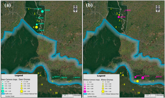
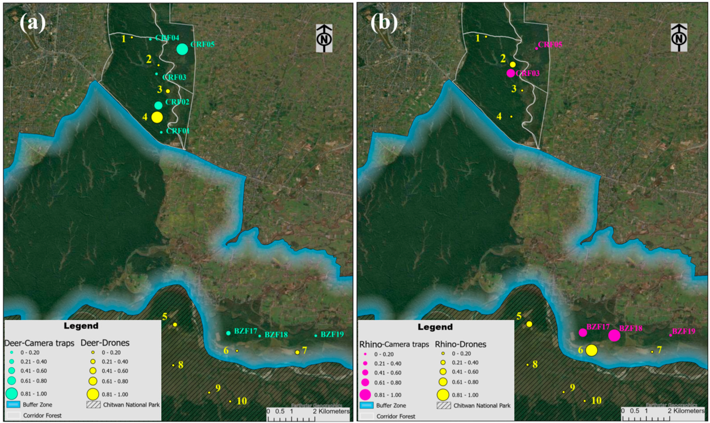
The normalized spatial indicators showed both correspondence and differences in wildlife distribution patterns between drone and camera trap observations (Figure 6). As shown in Figure 6a, deer activity exhibited spatial correspondence in several areas between the two monitoring platforms. The highest drone-derived activity was observed in Regions 4 and 3 within the Corridor Forest, and they were located near camera trap sites CRF02 and CRF03, which also showed relatively high or moderate normalized RAI values. The highest RAI value was observed at camera trap site CRF05, but this site was located away from the drone survey regions in the Corridor Forest. In the Buffer Zone, Region 7 showed relatively high drone-derived activity, whereas BZF17 showed relatively high camera trap-derived activity.

Figure 6. Spatial distribution of normalized drone-derived detection densities and normalized camera trap-derived RAI values for (a) deer and (b) rhinos. Drone survey regions are represented by centroid symbols sized according to normalized detection density, whereas camera trap sites are represented by symbols sized according to normalized RAI.

Rhino observations showed a similarly localized spatial pattern (Figure 6b). In the Buffer Zone, drone-derived rhino detections were mainly associated with Region 6, near BZF17 and BZF18, both of which had relatively high normalized RAI values. In the Corridor Forest, the highest normalized drone-derived density among the surveyed regions was observed in Region 2, near CRF03, which also showed a relatively high normalized RAI value.

Overall, the spatial alignment demonstrated some correspondence but not direct agreement between drone and camera trap observations, indicating both shared and differing species-specific spatial patterns across the two monitoring platforms.

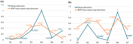
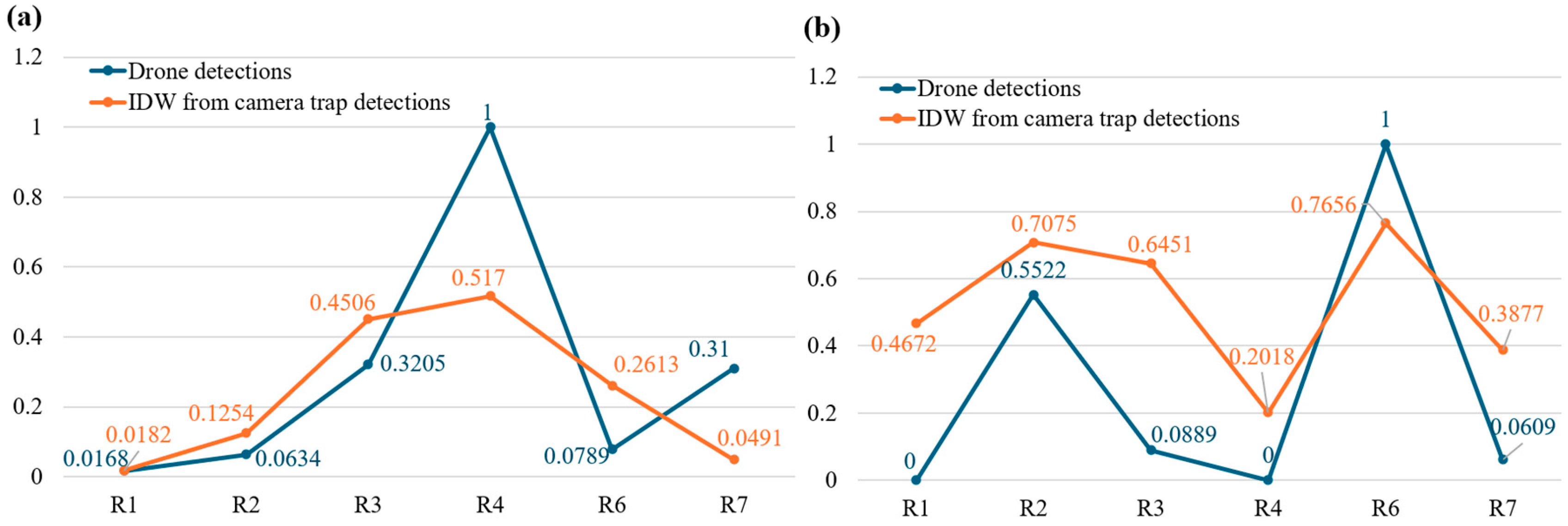
Figure 7 shows the cross-platform comparison across the drone survey regions. Figure 7a compares the deer activity patterns detected by drone and camera traps, which showed broadly similar spatial trends in the Corridor Forest between normalized drone-derived density and IDW-interpolated normalized camera trap RAI. Both drone-based and camera trap-derived results showed Region 4 (R4) as the highest-activity area and Region 1 (R1) as a low-activity area. The Corridor Forest regions showed a generally consistent increasing pattern from R1 to R4, although differences in relative magnitude were observed between the two platforms. In the Buffer Zone, however, Regions 6 and 7 showed contrasting patterns. R6 had a lower normalized drone-derived density than the IDW-interpolated camera trap RAI, whereas R7 showed a higher drone-derived density than the camera trap-derived value.

Figure 7. Cross-platform comparison of wildlife observations across drone survey regions for (a) deer and (b) rhinos. Camera trap observations are represented by IDW-interpolated normalized RAI values, while drone observations are represented by normalized drone-derived detection densities.

Figure 7b compares the rhino activity patterns detected by drone and camera traps. Despite differences in the relative magnitudes of the normalized values, both platforms showed a similar spatial trend across the six regions. Rhino activity increased from R1 to R2, decreased through R3 and R4, increased markedly at R6, and then declined at R7. Both platforms therefore identified R2 and R6 as regions of relatively high rhino activity, with R6 showing the highest normalized drone-derived density and a similarly high IDW-interpolated camera trap RAI.

Overall, the cross-platform comparison shows that drone and camera trap-based observations produced spatial correspondence in several regions, particularly in identifying relatively high-activity areas, while differences were also evident across some locations.

3.3.3. Cross-Platform Spatiotemporal Comparison

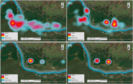
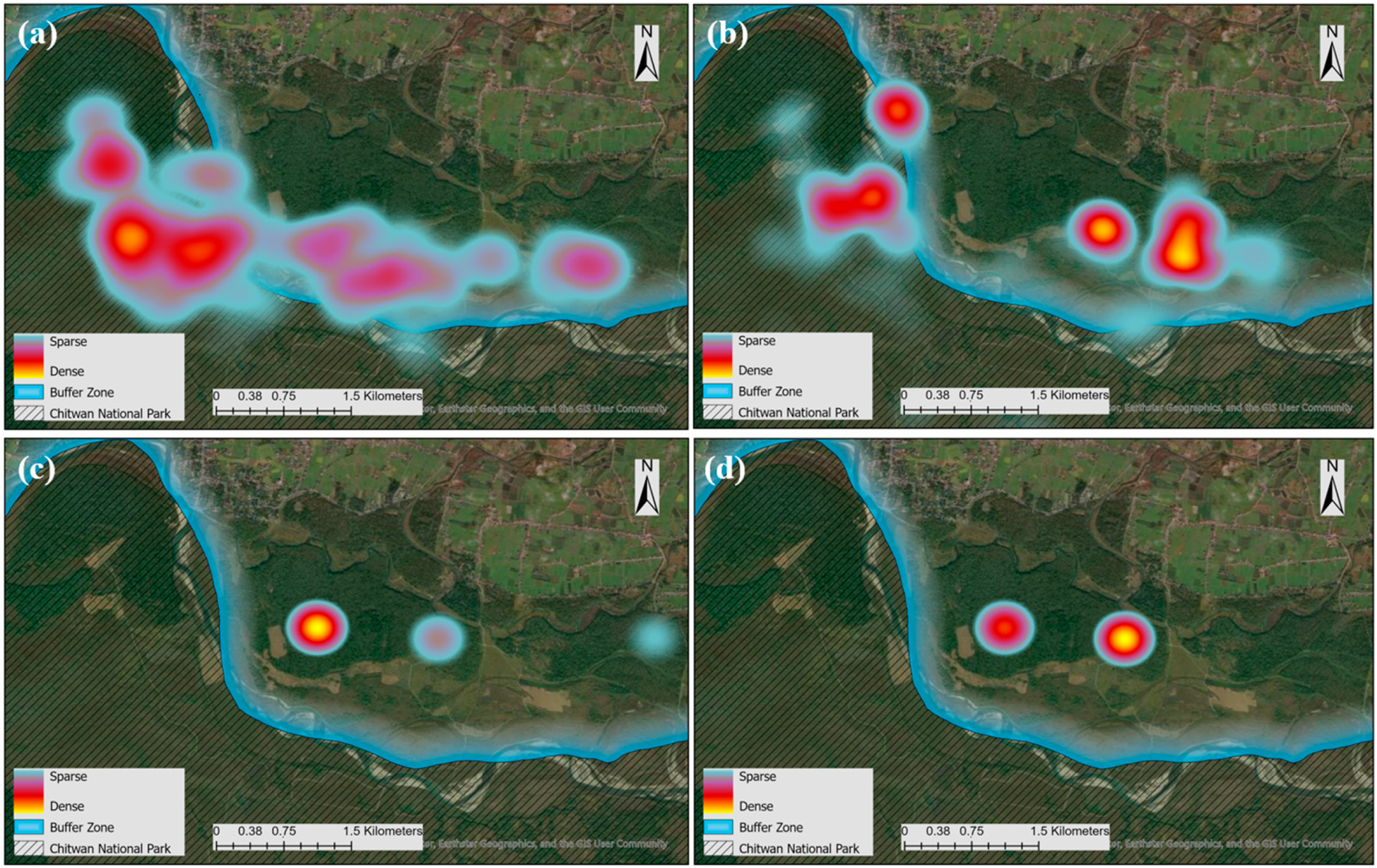
The KDE surfaces for May 2022 showed similar broad-scale spatial trends between drone and camera trap observations for both rhinos and deer (Figure 8). Drone-based rhino detections were concentrated mainly within CNP, with detection intensity decreasing from west to east (Figure 8a). Camera trap-derived rhino detections showed a similar west-to-east decline in activity (Figure 8c). This spatial correspondence suggests that both aerial and ground-based observations captured similar monthly distribution patterns for rhinos.

Figure 8. Kernel density maps of wildlife detections in May 2022, showing (a) drone-based rhino detections, (b) drone-based deer detections, (c) camera trap-based rhino detections, and (d) camera trap-based deer detections.

For deer, detections were concentrated mainly in the Buffer Zone, with higher activity in the eastern portion and lower activity in the western portion for both monitoring platforms (Figure 8b,d). These patterns showed spatial correspondence in the monthly distribution trends recorded by the two platforms.

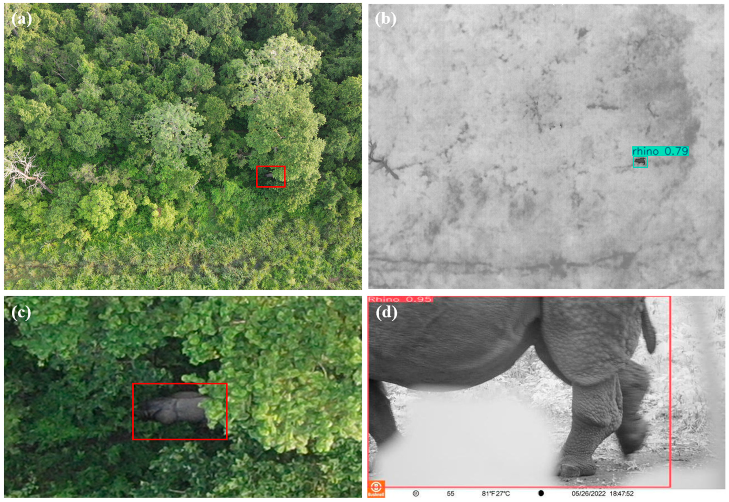
At a finer temporal scale, a one-day case study was examined for 26 May 2022, when drone and camera trap observations were acquired within a one-hour interval in the Buffer Zone. As shown in Figure 9, the deep learning model detected a rhino from the drone thermal imagery (Figure 9b), and the paired RGB images (Figure 9a,c) provided broader landscape context, partially showing the animal because of vegetation occlusion. Within only a one-hour interval, the deep learning model also identified a rhino from the camera trap imagery (Figure 9d), approximately 488 m from the detection location by drone. Although it cannot be confirmed that the drone and camera trap detections represented the same individual, their close temporal and spatial proximity provides cross-platform corroboration of rhino activity within the area.

Figure 9. Multi-perspective and multi-sensor rhino detection results acquired within a one-hour interval on 26 May 2022 and separated by approximately 488 m: (a) drone-collected RGB image for visual reference, (b) drone thermal detection, (c) zoomed-in drone RGB image showing additional detail, and (d) camera trap detection. Red boxes in (a,c) were manually added to indicate the rhino location.

4. Discussion

4.1. Deep Learning-Based Wildlife Detection

The deep learning experiments were conducted to select reliable detectors for subsequent spatial and spatiotemporal analyses rather than to provide an exhaustive benchmark of object-detection architectures. The two datasets presented different detection challenges. In camera trap images, animals were generally observed at closer range, occupied larger portions of the image, and retained more detailed shape and texture information. In contrast, animals in drone thermal images appeared as smaller top-down targets with limited visual detail and were sometimes affected by canopy obstruction and heterogeneous thermal backgrounds. Despite these differences, YOLOv11s maintained strong detection performance across both imaging perspectives and provided an appropriate accuracy–efficiency balance for generating the observations used in the subsequent analyses.

Radiometric variability among individual drone flights presents an additional source of uncertainty in thermal wildlife detection. Because the imagery was acquired under varying environmental conditions, animal–background thermal contrast could differ among flights as a result of changes in ambient temperature, solar heating, weather conditions, and time of day. Such variability can affect the appearance and visibility of animals in thermal imagery. To reduce this effect, surveys were conducted primarily during early morning or evening periods when thermal contrast between wildlife and the surrounding background was generally more favorable. Additionally, the training and test datasets contained thermal imagery acquired across multiple flights and environmental conditions. The strong test performance suggests that the deep learning models employed in this study were robust to radiometric variability presented in the collected dataset, although its flight-specific effect was not quantified.

Earlier wildlife-detection studies have applied both single-stage YOLO detectors and two-stage methods such as Faster R-CNN to aerial thermal imagery. Among these, our team developed an enhanced Faster R-CNN architecture to improve small-animal detection in drone thermal imagery through region proposals and multi-scale feature extraction [11]. In contrast, YOLO-based methods offer faster inference by performing localization and classification in a single stage, making them suitable for processing large volumes of drone imagery [7,10]. Recent studies have further demonstrated the ability of deep learning to locate animals in complex thermal scenes containing vegetation and partially obscured targets [12]. Consistent with these studies, our results indicate that YOLOv11s can provide reliable detections from both aerial thermal and ground-based camera trap imagery while retaining the computational efficiency required for large-scale offline image processing. Beyond detector selection, the main contribution of this study is the integration of detections derived from drones and camera traps in cross-platform spatial and spatiotemporal analyses to evaluate the distinct and complementary information provided by these two monitoring perspectives, a topic that has received relatively limited attention in previous wildlife-monitoring research.

4.2. Complementarity of Drone and Camera Trap Monitoring

The cross-platform analyses highlight the complementary value of drone and camera trap observations for wildlife monitoring. Although the two platforms differ fundamentally in sampling geometry, observation duration, and detection perspective, the correspondence in their relative spatial and spatiotemporal patterns suggests that they can capture a shared underlying signal of wildlife activity (Figure 6, Figure 7, Figure 8 and Figure 9). Drone surveys provide spatially extensive observations over defined areas at particular times, whereas camera traps provide repeated observations from fixed locations over longer periods. Integrating these perspectives therefore provides information across spatial and temporal dimensions that cannot be obtained as effectively from either platform alone.

Importantly, the normalized drone density and camera trap RAI should not be interpreted as equivalent measures of abundance. Normalization facilitates comparison of relative spatial patterns, but the two indicators remain products of different sampling processes. Drone-derived density reflects the number of animals visible within an aerial survey footprint during a relatively short observation period, whereas camera trap RAI reflects the frequency of independent detections accumulated at fixed sites over time. Consequently, differences in the magnitude of the normalized indicators at individual locations are expected and do not necessarily indicate inconsistency between the platforms. Rather, agreement in broader spatial trends is more informative for evaluating whether the two monitoring perspectives identify similar areas of wildlife activity.

The KDE comparison and the finer-scale rhino case further illustrate this complementarity from different temporal perspectives (Figure 8 and Figure 9). The monthly comparison indicates that the two platforms can recover similar broad distribution patterns despite their different sampling designs, while the fine-scale case demonstrates how observations from separate sensors can provide mutually supporting evidence of wildlife presence within a restricted spatial and temporal context. At the same time, such correspondence should be interpreted as cross-platform corroboration rather than confirmation that the same individual animal was observed. Together, these findings support the use of drones and camera traps as complementary components of a multi-perspective monitoring strategy, with aerial observations extending spatial coverage and ground-based observations providing repeated, close-range records over longer periods.

4.3. Interpretation of Deer Patterns in the Buffer Zone

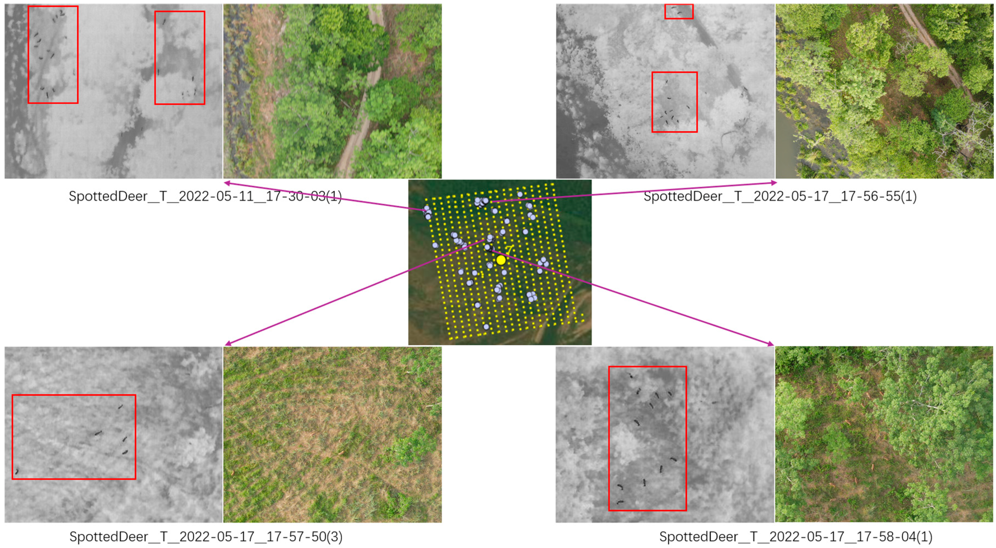
A notable discrepancy between the two monitoring platforms occurred in Regions 6 and 7 of the Buffer Zone, where the relative deer activity patterns were reversed between drone- and camera trap-derived observations (Figure 7a). One factor that may contribute to this difference is the spatial aggregation of deer within the drone imagery. In R6, 60 deer detections occurred across 38 deer-positive images, corresponding to a mean of 1.58 detections per positive image. In R7, 225 deer detections occurred across 89 deer-positive images, corresponding to a higher mean of 2.53 detections per positive image. Because drone-derived density is influenced by the number of individuals detected within the survey footprint at the time of image acquisition, greater aggregation can increase the observed density even when the number of occupied locations is limited. In contrast, camera trap RAI is based on independent detection events accumulated over time at fixed sites and therefore responds differently to short-term grouping behavior.

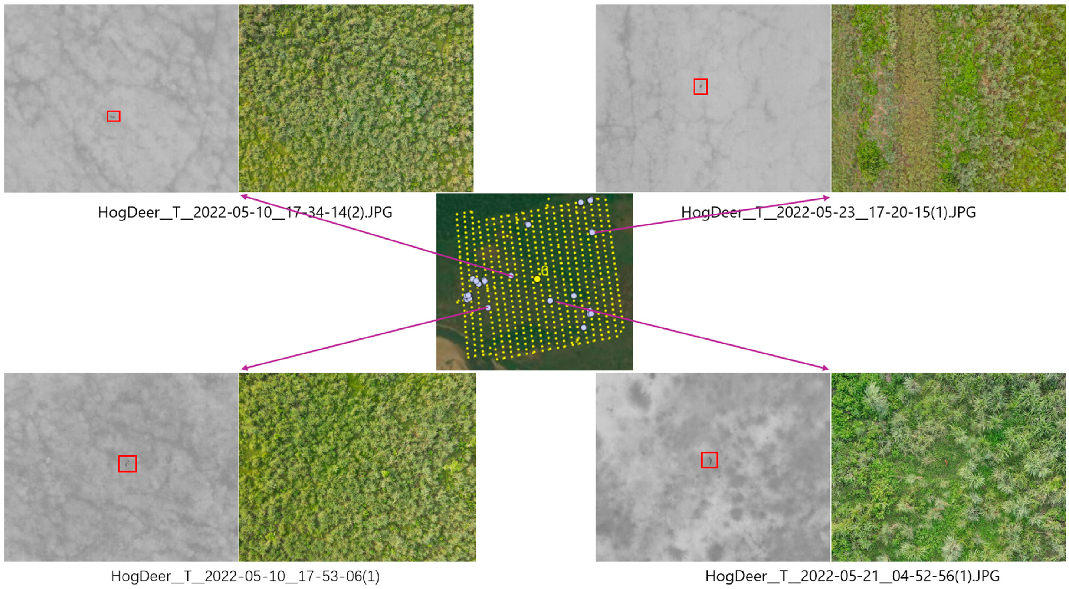
Visual examination of the paired thermal and RGB imagery provided additional ecological context for this contrast. Deer in R6 generally appeared as single individuals, whereas multiple individuals were more frequently observed together in R7 (Figure 10 and Figure 11), which is consistent with the quantitative aggregation analysis. The representative imagery also showed hog deer in R6 and spotted deer in R7. However, because the drone detection model used a single deer class and species composition was not systematically quantified across all detections, these species-level observations cannot be used to attribute the regional difference directly to species-specific behavior. They instead provide qualitative context for the observed aggregation patterns.

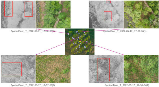
Figure 10. Visual examination of drone-derived deer detections in Region 6 using paired thermal and RGB imagery. The center panel shows drone image footprints and deer detection locations; yellow points represent drone image footprints, and light-blue points indicate images containing deer detections. The surrounding panels show paired thermal and RGB images, with detected deer highlighted by red boxes.

Figure 11. Visual examination of drone-derived deer detections in Region 7 using paired thermal and RGB imagery. The representative image pairs show multiple deer frequently occurring within single images in riverine and forested habitat.

Landscape conditions may also contribute to differences in how deer are distributed and detected. The paired RGB imagery showed that R6 was dominated by tall grassland, whereas R7 included more riverine and forested habitats (Figure 10 and Figure 11). Such differences in vegetation structure could affect both animal use of the landscape and visibility from an aerial perspective. However, because vegetation cover was not quantitatively classified in this study, these habitat differences should be interpreted as contextual observations rather than confirmed explanatory factors. The contrasting R6–R7 patterns therefore likely reflect a combination of within-image deer aggregation, local ecological conditions, and the fundamentally different spatial and temporal sampling characteristics of drone and camera trap monitoring.

5. Conclusions

This study integrates drone-based thermal imagery, paired RGB imagery, and camera trap imagery within a multi-perspective wildlife monitoring approach, with deep learning methods used to support automated detection. Among the evaluated models, YOLOv11s achieved the strongest overall performance on both the drone thermal and camera trap datasets, demonstrating its effectiveness for wildlife detection across aerial and ground-based imagery. For deer and rhinos, the two species shared by both datasets, cross-platform spatial and spatiotemporal analyses showed broad correspondence in wildlife distribution patterns while also revealing local differences between aerial and ground-based observations. These findings highlight the complementary value of the two monitoring perspectives rather than direct equivalence between their platform-specific activity measures. Drone-based thermal imagery improves detectability across broad areas, drone-based RGB imagery provides valuable environmental context, and camera traps offer close-range observational detail over longer periods.

Taken together, these findings indicate that integrating aerial and ground-based sensing with deep learning provides a practical multi-perspective approach for wildlife monitoring in heterogeneous protected landscapes. This study used a DJI Mavic 2 Enterprise Advanced with its integrated RGB–thermal imaging system; therefore, the transferability of the monitoring approach across different drone platforms and sensor systems remains to be evaluated. Future work should incorporate a broader range of species and apply advanced spatiotemporal interaction models to further evaluate species distributions, temporal dynamics, and the capacity of multi-perspective monitoring to characterize wildlife patterns across complex landscapes.

References

- Pollock, K.H.; Nichols, J.D.; Simons, T.R.; Farnsworth, G.L.; Bailey, L.L.; Sauer, J.R. Large-scale wildlife monitoring studies: Statistical methods for design and analysis. Environmetrics 2002, 13, 105–119. [Google Scholar] [CrossRef] [Scilit]
- Hodgson, J.C.; Baylis, S.M.; Mott, R.; Herrod, A.; Clarke, R.H. Precision wildlife monitoring using unmanned aerial vehicles. Sci. Rep. 2016, 6, 22574. [Google Scholar] [CrossRef] [Scilit]
- Linchant, J.; Lisein, J.; Semeki, J.; Lejeune, P.; Vermeulen, C. Are unmanned aircraft systems (UAS) the future of wildlife monitoring? A review of accomplishments and challenges. Mammal. Rev. 2015, 45, 239–252. [Google Scholar] [CrossRef] [Scilit]
- Sharma, S.; Sato, K.; Gautam, B.P. A methodological literature review of acoustic wildlife monitoring using artificial intelligence tools and techniques. Sustainability 2023, 15, 7128. [Google Scholar] [CrossRef] [Scilit]
- Corcoran, E.; Winsen, M.; Sudholz, A.; Hamilton, G. Automated detection of wildlife using drones: Synthesis, opportunities and constraints. Methods Ecol. Evol. 2021, 12, 1103–1114. [Google Scholar] [CrossRef] [Scilit]
- Koger, B.; Deshpande, A.; Kerby, J.T.; Graving, J.M.; Costelloe, B.R.; Couzin, I.D. Quantifying the movement, behaviour and environmental context of group-living animals using drones and computer vision. J. Anim. Ecol. 2023, 92, 1357–1371. [Google Scholar] [CrossRef] [Scilit]
- Lee, S.; Song, Y.; Kil, S.H. Feasibility analysis of real-time detection of wildlife using drone-derived thermal and RGB images. Remote Sens. 2021, 13, 2169. [Google Scholar] [CrossRef] [Scilit]
- Beaver, J.T.; Baldwin, R.W.; Messinger, M.; Newbolt, C.H.; Ditchkoff, S.S.; Silman, M.R. Evaluating the use of drones equipped with thermal sensors as an effective method for estimating wildlife. Wildl. Soc. Bull. 2020, 44, 434–443. [Google Scholar] [CrossRef] [Scilit]
- Besson, M.; Alison, J.; Bjerge, K.; Gorochowski, T.E.; Høye, T.T.; Jucker, T.; Clements, C.F. Towards the fully automated monitoring of ecological communities. Ecol. Lett. 2022, 25, 2753–2775. [Google Scholar] [CrossRef] [Scilit]
- Povlsen, P.; Bruhn, D.; Durdevic, P.; Arroyo, D.O.; Pertoldi, C. Using YOLO object detection to identify hare and roe deer in thermal aerial video footage—Possible future applications in real-time automatic drone surveillance and wildlife monitoring. Drones 2023, 8, 2. [Google Scholar] [CrossRef] [Scilit]
- Lyu, H.; Qiu, F.; An, L.; Stow, D.; Lewison, R.; Bohnett, E. Deer survey from drone thermal imagery using enhanced Faster R-CNN based on ResNets and FPN. Ecol. Inform. 2024, 79, 102383. [Google Scholar] [CrossRef] [Scilit]
- Backman, K.; Wood, J.; Brandimarti, M.; Beranek, C.T.; Roff, A. Human inspired deep learning to locate and classify terrestrial and arboreal animals in thermal drone surveys. Methods Ecol. Evol. 2025, 16, 1239–1254. [Google Scholar] [CrossRef] [Scilit]
- Aliane, N. Drones and AI-driven solutions for wildlife monitoring. Drones 2025, 9, 455. [Google Scholar] [CrossRef] [Scilit]
- Gao, P.; Zhong, D.; Qi, Q.; Ling, C.; Qiu, C.; Wang, B.; Du, X.; Gao, M. FDM-YOLO: Real-time small-target UAV wildlife detection via attention-guided cross-modality fusion. Ecol. Inform. 2026, 95, 103697. [Google Scholar] [CrossRef] [Scilit]
- Lundquist, U.P.S.; Afridi, S.; Berthelot, C.; Dat, N.N.; Hlebowicz, K.; Iannino, E.; Laporte-Devylder, L.; Maalouf, G.; May, G.; Meier, K.; et al. WildDrone: Autonomous drone technology for monitoring wildlife populations. Front. Robot. AI 2026, 12, 1695319. [Google Scholar] [CrossRef] [Scilit]
- Caravaggi, A.; Banks, P.B.; Burton, A.C.; Finlay, C.M.; Haswell, P.M.; Hayward, M.W.; Wood, M.D. A review of camera trapping for conservation behaviour research. Remote Sens. Ecol. Conserv. 2017, 3, 109–122. [Google Scholar] [CrossRef] [Scilit]
- Linkie, M.; Ridout, M.S. Assessing tiger-prey interactions in Sumatran rainforests. J. Zool. 2011, 284, 224–229. [Google Scholar] [CrossRef] [Scilit]
- Pierini, S.E.; Simoncini, M.S.; Larriera, A.; Guarascio, V.F.V.; Scarpa, L.J.; Piña, C.I. Camera-traps detect the maned wolf preying on broad-snouted caiman eggs. Glob. Ecol. Conserv. 2024, 51, e02916. [Google Scholar] [CrossRef] [Scilit]
- Rowcliffe, J.M.; Field, J.; Turvey, S.T.; Carbone, C. Estimating animal density using camera traps without the need for individual recognition. J. Appl. Ecol. 2008, 45, 1228–1236. [Google Scholar] [CrossRef] [Scilit]
- Tanwar, K.S.; Sadhu, A.; Jhala, Y.V. Camera trap placement for evaluating species richness, abundance, and activity. Sci. Rep. 2021, 11, 23050. [Google Scholar] [CrossRef] [Scilit]
- Jasiulionis, M.; Stirkė, V.; Balčiauskas, L. The distribution and activity of the invasive raccoon dog in Lithuania as found with country-wide camera trapping. Forests 2023, 14, 1328. [Google Scholar] [CrossRef] [Scilit]
- Palmer, M.S.; Swanson, A.; Kosmala, M.; Arnold, T.; Packer, C. Evaluating relative abundance indices for terrestrial herbivores from large-scale camera trap surveys. Afr. J. Ecol. 2018, 56, 791–803. [Google Scholar] [CrossRef] [Scilit]
- Himeur, Y.; Rimal, B.; Tiwary, A.; Amira, A. Using artificial intelligence and data fusion for environmental monitoring: A review and future perspectives. Inf. Fusion. 2022, 86, 44–75. [Google Scholar] [CrossRef] [Scilit]
- Hyde, P.; Dubayah, R.; Walker, W.; Blair, J.B.; Hofton, M.; Hunsaker, C. Mapping forest structure for wildlife habitat analysis using multi-sensor (LiDAR, SAR/InSAR, ETM+, QuickBird) synergy. Remote Sens. Environ. 2006, 102, 63–73. [Google Scholar] [CrossRef] [Scilit]
- Brum-Bastos, V.; Long, J.; Church, K.; Robson, G.; de Paula, R.; Demšar, U. Multi-source data fusion of optical satellite imagery to characterize habitat selection from wildlife tracking data. Ecol. Inform. 2020, 60, 101149. [Google Scholar] [CrossRef] [Scilit]
- Hajder, M.; Kolbusz, J.; Liput, M. An AI-based integrated multi-sensor system with edge computing for the adaptive management of human–wildlife conflict. Sensors 2025, 25, 6415. [Google Scholar] [CrossRef] [Scilit]
- Wild, T.A.; van Schalkwyk, L.; Viljoen, P.; Heine, G.; Richter, N.; Vorneweg, B.; Wikelski, M. A multi-species evaluation of digital wildlife monitoring using the Sigfox IoT network. Anim. Biotelemetry 2023, 11, 13. [Google Scholar] [CrossRef] [Scilit]
- Gottwald, J.; Lampe, P.; Höchst, J.; Friess, N.; Maier, J.; Leister, L.; Nauss, T. BatRack: An open-source multi-sensor device for wildlife research. Methods Ecol. Evol. 2021, 12, 1867–1874. [Google Scholar] [CrossRef] [Scilit]
- Mishra, H.R. Balancing human needs and conservation in Nepal’s Royal Chitwan Park. Ambio 1982, 11, 246–251. [Google Scholar]
- Dai, J.; Roberts, D.A.; Stow, D.A.; An, L.; Hall, S.J.; Yabiku, S.T.; Kyriakidis, P.C. Mapping understory invasive plant species with field and remotely sensed data in Chitwan, Nepal. Remote Sens. Environ. 2020, 250, 112037. [Google Scholar] [CrossRef] [Scilit]
- Baidya, N.G.; Bhuju, D.R.; Kandel, P. Land use change in buffer zone of Chitwan National Park, Nepal between 1978 and 1999. Ecoprint 2009, 16, 79–86. [Google Scholar] [CrossRef] [Scilit]
- Dangol, D.; Ghimire, A.; Bhattarai, S.B. Human–elephant conflict in the buffer zone of Chitwan National Park, Nepal. Nepal. J. Zool. 2020, 4, 36–43. [Google Scholar] [CrossRef] [Scilit]
- Lamichhane, S.; Gurung, A.; Pokheral, C.P.; Rayamajhi, T.; Gotame, P.; Regmi, P.R.; Lamichhane, B.R. First record of the Dhole Cuon alpinus (Mammalia: Carnivora: Canidae) in Barandabhar Corridor Forest, Chitwan, Nepal. J. Threat. Taxa 2018, 10, 11243–11244. [Google Scholar] [CrossRef] [Scilit]
- Smith, A.C.; Hurni, K.; Fox, J.; Van Den Hoek, J. Community Forest management led to rapid local forest gain in Nepal: A 29-year mixed methods retrospective case study. Land. Use Policy 2023, 126, 106526. [Google Scholar] [CrossRef] [Scilit]
- Roboflow. Computer Vision Tools for Developers and Enterprises. Available online: https://roboflow.com (accessed on 14 March 2025).
- Bjerge, K.; Alison, J.; Dyrmann, M.; Frigaard, C.E.; Mann, H.M.; Høye, T.T. Accurate detection and identification of insects from camera trap images with deep learning. PLoS Sustain. Transform. 2023, 2, e0000051. [Google Scholar] [CrossRef] [Scilit]
- Leonid, T.T.; Kanna, H.; VJ, C.C.; Hamritha, A.S.; Lokesh, C. Human-wildlife conflict mitigation using YOLO algorithm. In Proceedings of the 2023 Eighth International Conference on Science Technology Engineering and Mathematics (ICONSTEM); IEEE: Piscataway, NJ, USA, 2023; pp. 1–7. [Google Scholar] [CrossRef] [Scilit]
- Chen, H.; Qiu, F.; Kulsum, U.; Zhang, C.; Bohnett, E.; Lyu, H.; Tian, S.; Lamichhane, B.R.; Stow, D.; Lewison, R.; et al. Deep learning-based monitoring and spatiotemporal analysis of wildlife and human activities using camera trap imagery. Eur. J. Wildl. Res. 2026, 72, 122. [Google Scholar] [CrossRef] [Scilit]
- Talaat, F.M.; ZainEldin, H. An improved fire detection approach based on YOLOv8 for smart cities. Neural Comput. Appl. 2023, 35, 20939–20954. [Google Scholar] [CrossRef] [Scilit]
- Khanam, R.; Hussain, M. YOLOv11: An overview of the key architectural enhancements. arXiv 2024, arXiv:2410.17725. [Google Scholar] [CrossRef] [Scilit]
- Rovero, F.; Marshall, A.R. Camera trapping photographic rate as an index of density in forest ungulates. J. Appl. Ecol. 2009, 46, 1011–1017. [Google Scholar] [CrossRef] [Scilit]
- Ngoprasert, D.; Lynam, A.J.; Gale, G.A. Human disturbance affects habitat use and behaviour of Asiatic leopard Panthera pardus in Kaeng Krachan National Park, Thailand. Oryx 2007, 41, 343–351. [Google Scholar] [CrossRef] [Scilit]
- Wentzel, J.; Gall, C.; Bourn, M.; De Beer, J.; Du Plessis, F.; Fosgate, G.T. Carnivore detection at the domestic/wildlife interface within Mpumalanga Province, South Africa. Animals 2021, 11, 2535. [Google Scholar] [CrossRef] [Scilit]
- Bagheriyan, E.; Karimi, A.; Yazdandad, H. Assessing spatiotemporal patterns of human–wildlife conflicts in a human-dominated landscape: A case study from Iran. Biodivers. Conserv. 2023, 32, 4239–4257. [Google Scholar] [CrossRef] [Scilit]
- Ahmad, F.; Mori, T.; Rehan, M.; Bosso, L.; Kabir, M. Applying a random encounter model to estimate the Asiatic black bear (Ursus thibetanus) density from camera traps in the Hindu Raj Mountains, Pakistan. Biology 2024, 13, 341. [Google Scholar] [CrossRef] [Scilit]
Disclaimer/Publisher’s Note: The statements, opinions and data contained in all publications are solely those of the individual author(s) and contributor(s) and not of MDPI and/or the editor(s). MDPI and/or the editor(s) disclaim responsibility for any injury to people or property resulting from any ideas, methods, instructions or products referred to in the content. |
© 2026 by the authors. Licensee MDPI, Basel, Switzerland. This article is an open access article distributed under the terms and conditions of the Creative Commons Attribution (CC BY) license.