


Highlights
What are the main findings?
- 3D-GIGAMO integrates real-patch-guided implicit minority-class augmentation with a hybrid CNN–Transformer classifier for class-imbalanced HSI classification.
- On four public benchmarks, 3D-GIGAMO achieves average accuracies of 99.58%, 98.45%, 96.88%, and 99.85%, respectively, outperforming several recent methods.
What are the implications of the main findings?
- Classifier-oriented minority-class augmentation can effectively alleviate class imbalance and improve minority-class recognition under limited labeled samples.
- Joint learning with real and synthesized samples provides an effective framework for class-balanced HSI classification.
Abstract
Hyperspectral image (HSI) classification is important for land-cover recognition and remote-sensing scene analysis. However, class imbalance severely limits performance when minority classes contain only a few labeled samples, causing models to show strong overall results while failing to identify minority classes effectively. We propose a 3D guided implicit generative adversarial oversampling model (3D-GIGAMO), a generation–classification collaborative framework that alleviates class imbalance by producing class-conditioned minority-class patches for task-oriented oversampling, while learning discriminative spectral–spatial representations for robust and class-balanced HSI classification. A guided implicit neural representation conditioned on real training patches is embedded in an adversarial learning framework, and optimization is regularized using a conditional bounded-score objective with gradient-norm regularization. A hybrid convolutional neural network (CNN)–Transformer classifier is trained on both real and synthesized patches, and a class-consistency loss encourages the synthesized patches to preserve target-class semantics. Experiments on four public benchmarks (Indian Pines, Pavia University, WHU-Hi-LongKou, and Salinas) show improvements in both overall and average accuracy across all datasets, achieving average accuracies of 99.58%, 98.45%, 96.88%, and 99.85%, respectively, outperforming several recent methods.
1. Introduction
With rich spectral–spatial information and finer material separability than RGB or multispectral data, hyperspectral images (HSIs) are suitable for land-cover classification [1,2].
Image classification is one of the most important approaches for extracting land-cover information from HSIs [3,4]. Initial research on HSI classification primarily used conventional machine-learning approaches, including random forest (RF) [5,6] and logistic regression [7]. Although effective to some extent, these methods depended heavily on hand-crafted features and were limited in modeling spatial structures in HSIs.
To overcome the limitations of hand-crafted features, deep learning approaches have been broadly applied to HSI classification [8,9,10,11]. Early studies mainly relied on 2D CNNs [12] and 3D CNNs [13] to capture spatial or joint spectral–spatial information. Recent methods have further enhanced feature representation through advanced convolutional, multiscale, and sequence-modeling strategies. For example, Zhai and Zhao [14] developed a two-stream spectral–spatial architecture; Jiang et al. [15] proposed S2WaveNet to strengthen spectral–spatial feature modeling; Zhang et al. [16] introduced a multi-level deformable gated aggregation network. Meanwhile, recent sequence-modeling studies [17,18] further improved spectral–spatial representation learning by enhancing local contextual modeling and long-range dependency capture. Beyond HSI classification, deep learning has also been extended to broader hyperspectral image-processing tasks. The sliding dual-window-inspired reconstruction network [19] exploits contextual information for hyperspectral anomaly detection, while the nonlocal and local feature-coupled self-supervised network [20] enhances representation learning by jointly modeling local and nonlocal features. In addition, spectral-prior-guided object detection [21] incorporates spectral priors to strengthen target discrimination in hyperspectral remote sensing imagery. The visible-light-to-hyperspectral cross-domain detection network (VHCDN) [22] extracts domain-shared spatial features and models spectral uncertainty for hyperspectral object detection. These studies further demonstrate the importance of effectively exploiting spatial, spectral, and contextual information in hyperspectral representation learning.
Despite great advances in deep learning, imbalanced class distributions seriously impede practical HSI classification. Models tend to favor majority classes, yielding high overall accuracy (OA) yet poor minority-class performance and lower average accuracy (AA) [23]. To address this issue, sampling-based strategies such as undersampling [24], oversampling [25], and hybrid methods [26] have been widely adopted. Some studies further combine imbalance-aware oversampling with dedicated classifiers. For example, Datta et al. [27] used PCA, ADASYN, and a refined deep subsampled multi-scale cascaded forest to improve minority-class recognition. However, these methods still mainly rely on conventional resampling rules and classifier-level optimization, which are insufficient to characterize the complex spectral–spatial distribution of minority classes. Consequently, they often suffer from overfitting and redundant samples in real applications [28], motivating the development of generative oversampling methods for task-oriented minority-class augmentation.
Implicit neural representation (INR) models data as continuous functions by learning mappings from coordinates to signals [29] and has demonstrated strong representation capability in image super-resolution [30] and 3D reconstruction [31]. For minority-class hyperspectral samples, even when only a limited number of training patches are available, each patch still contains rich internal spectral–spatial correlations. The continuous coordinate-based modeling of INR can exploit such internal information and provide a more informative spectral–spatial representation for minority-class sample generation. In contrast, conventional noise-driven oversampling methods based on generative adversarial networks (GAN) mainly generate samples from random latent variables [32] and may not sufficiently utilize the internal spectral–spatial information contained in real minority-class samples when training data are scarce, which limits effective modeling of minority-class characteristics. Building upon GAMO [33], this paper proposes a novel 3D Guided Implicit Generative Adversarial Oversampling Model (3D-GIGAMO) for class-imbalanced HSI classification. The proposed framework combines INR with adversarial learning and introduces real minority-class HSI patches to guide the generation process. This enables the generator to exploit the internal spectral–spatial information of real samples through implicit representation while adversarial learning further constrains the synthesized samples. Meanwhile, the classifier provides class-consistency supervision to encourage the generated samples to preserve discriminative information of the target class and is trained using both real and synthesized samples. Consequently, minority-class samples contribute more effectively to model optimization, thereby alleviating majority-class bias caused by class imbalance. The contributions are listed below:
- A guided implicit neural representation (GINR) is developed by integrating coordinate-based generation with real-patch guidance to produce class-conditioned minority samples for task-oriented oversampling.
- A unified multiscale reweighting strategy is proposed for effective multiscale feature modeling in both the generator and the classifier.
- A Gaussian semantic token aggregator (GSTA) is introduced to compact spatial features into semantic tokens, reducing redundancy and improving modeling efficiency.
- A residual-enhanced transformer block (RETB) is proposed to strengthen long-range semantic dependency modeling and improve spectral–spatial representations.
The remainder of this paper is organized as follows. Section 2 presents the proposed 3D-GIGAMO framework, including patch extraction, guided implicit generation, conditional discrimination, the HCT classifier, and the training objectives. Section 3 describes the datasets and experimental settings and reports the classification results and computational costs. Section 4 discusses the ablation and sensitivity analyses. Section 5 concludes the paper and discusses the limitations and directions for future work.
2. Materials and Methods
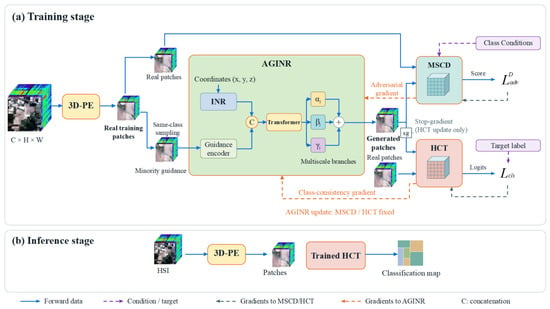
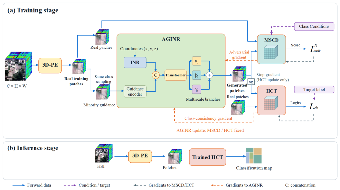
This section presents the proposed 3D-GIGAMO framework (Figure 1) for HSI classification. The framework contains four key modules: (1) a 3D patch extraction (3D-PE) module that partitions the HSI cube into local spectral–spatial patches; (2) a generator based on adaptive guided implicit neural representation (AGINR), responsible for producing class-conditioned minority-class patches for classifier-oriented augmentation; (3) a multiscale conditional discriminator (MSCD) that integrates 3D/2D convolutions with MLP structures to assess the class-conditional compatibility of generated samples with the learned training representation; and (4) a Hybrid CNN–Transformer (HCT) classifier that jointly models local spectral–spatial representations and long-range contextual relationships. This classifier enhances classification accuracy while enforcing a class-consistency constraint on the generator, guiding it to synthesize more discriminative minority-class samples.
Figure 1.
Illustration of our proposed 3D-GIGAMO, consisting of a 3D-PE module, an AGINR module, an MSCD module, and an HCT module.
To jointly optimize these modules, we adopt conditional bounded-score adversarial learning with gradient-norm regularization. Under the supervision of the discriminator and classifier, the generator learns class-conditioned, task-relevant minority samples, while the classifier learns from both real and generated data to enhance minority-class recognition. This joint training strategy mitigates class imbalance and improves overall classification performance.
2.1. 3D Patch Extractor
An HSI can be represented as a 3D hyperspectral tensor of size , denoted by . HSI classification aims to assign each pixel to one of U predefined land-cover categories, with the class index set defined as . Specifically, each pixel corresponds to a -dimensional spectral vector , where and .
Before patch extraction, PCA is applied along the spectral dimension to reduce the original HSI to 30 principal components, producing , where . Subsequently, 3D HSI patches are extracted from using a sliding window with a stride of 1, where denotes the spatial neighborhood and C denotes the number of retained principal components. These patches are used as inputs to the proposed 3D-GIGAMO network.
2.2. Adaptive Guided Implicit Neural Representation Generator
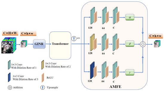
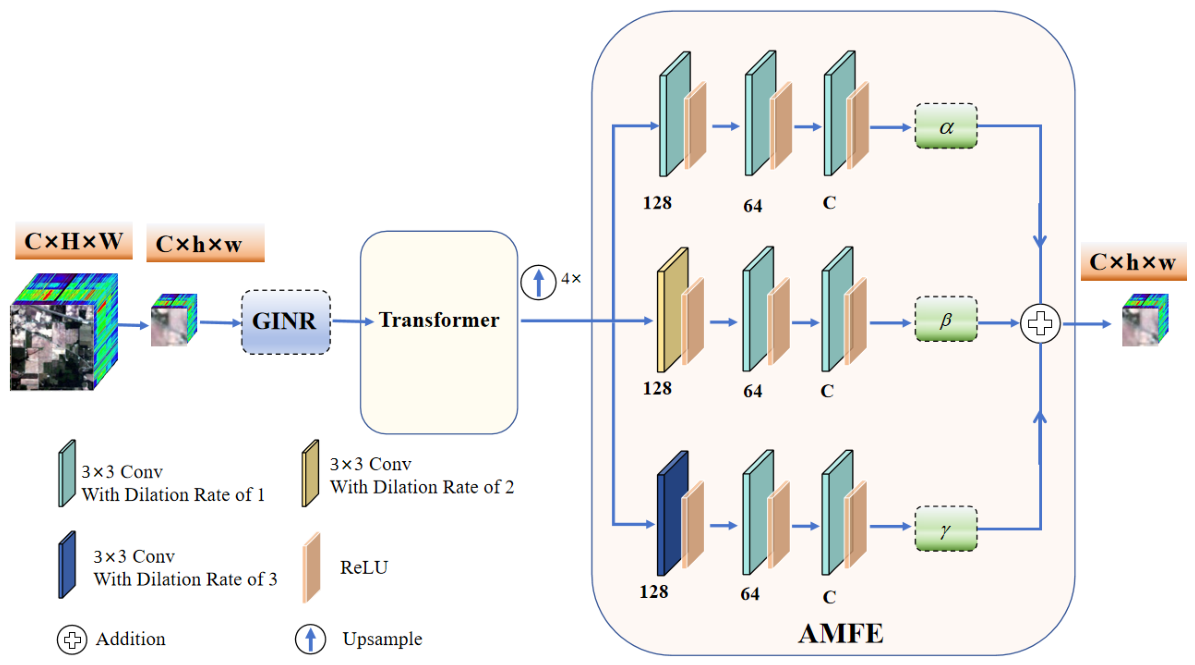
AGINR (Figure 2) serves as the generative core of 3D-GIGAMO and is designed to provide task-oriented minority-class augmentation. Unlike conventional oversampling driven only by random noise, AGINR introduces a real-sample-guided implicit representation to condition the generation process and preserve task-relevant spectral–spatial information. It consists of three components: (1) a Guided Implicit Neural Representation (GINR) module for coordinate-based generation conditioned on minority-class training patches; (2) a Transformer-based global feature modeling module for capturing long-range contextual dependencies and enhancing global semantic coherence; and (3) an Adaptive Multiscale Feature Extraction (AMFE) module for adaptively integrating multiscale contextual information to generate more discriminative minority-class patches.
Figure 2.
The structure of AGINR.
2.2.1. Guided Implicit Neural Representation
Compared with conventional INR without real-sample guidance, the proposed GINR uses minority-class training patches to condition coordinate-based synthesis and retain information relevant to class discrimination. Following the preprocessing described in the 3D Patch Extractor, GINR generates minority-class patches with the same dimensionality as the real training patches. These generated patches are used for classifier-oriented augmentation rather than for reconstructing the original reflectance spectra. Among U classes, the one having the highest sample count becomes the majority class, leaving the remaining as minority classes. For each minority class j (), an independent parameter set is learned to construct a GINR, formulated as:
where represents the GINR for the j-th minority class, represents its learnable parameters, and is the generated spectral value. The variables x, y, and z represent the spatial–spectral coordinates of the generated minority-class HSI patches, where , , and .
Let denote the generated samples count for the j-th minority class, defined as:
where and denote the counts of majority-class training samples and j-th minority-class real samples, respectively.
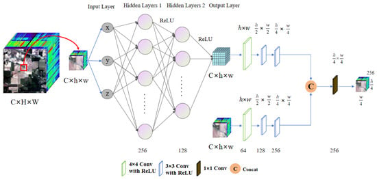
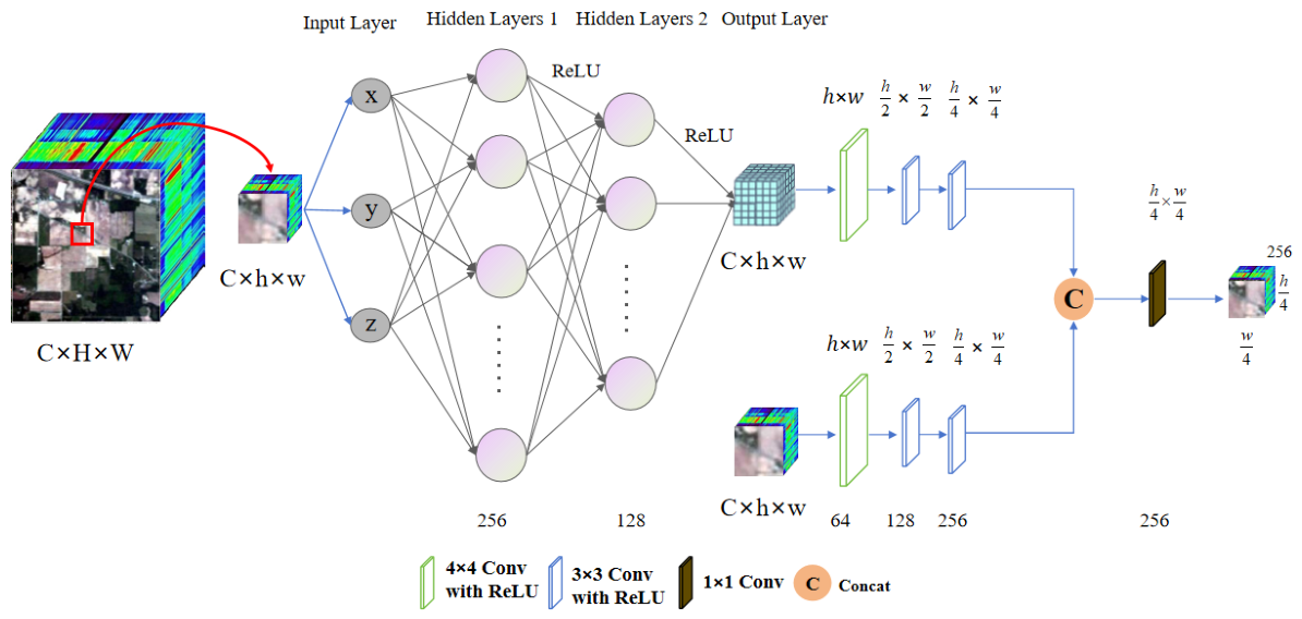
As shown in Figure 3, GINR consists of an Implicit-Generation Module (IGM) and a Generator-Guidance Module (GGM). The IGM is implemented as an MLP that maps the 3D coordinate vector to HSI pixel values. The network includes two ReLU-based fully connected hidden layers with 256 and 128 neurons, followed by a one-neuron output layer for predicting the HSI pixel value at the given coordinate. A complete minority-class HSI patch is generated by predicting all spectral values over spatial locations.
Figure 3.
The structure of GINR.
For each minority class, real guidance patches are drawn with replacement from its training samples, and their count is set equal to the generated-patch count in the current iteration. The synthetic minority-class patches are not pre-generated and fixed before training; instead, they are dynamically regenerated at each training iteration using the current generator parameters and newly resampled real guidance patches. Based on these paired generated and real samples, the GGM is designed to exploit their complementary information. Specifically, the minority-class HSI patch generated by the IGM and the corresponding real guidance patch are fed into two structurally identical 2D convolutional encoders for high-level feature extraction. Each encoder comprises three convolutional layers using and kernels, with stride-2 operations enabling two-stage spatial downsampling. This design preserves rich semantic information while producing more abstract features with lower spatial resolution, thus improving computational efficiency and generalization. After channel-wise concatenation, the extracted features enter a convolutional fusion encoder for dimension reduction and semantic integration, yielding a unified joint feature representation for subsequent global modeling and contextual reconstruction.
Let denote the feature representation of the generated sample, and let denote that of the guidance sample, where B is the batch size and is the number of feature channels. The fusion process is formulated as:
Importantly, the real training patches in AGINR serve as conditional guidance rather than direct reconstruction targets. Since the generated and guidance patches are processed through separate feature extraction paths and fused only at the feature level, the synthesized patch is not obtained by directly reproducing a selected guidance sample. This design reduces the dependence of the generation process on individual guidance patches and, to some extent, mitigates the risk of overfitting. Nevertheless, under extremely few-shot conditions, the diversity of the available guidance information remains inherently limited.
2.2.2. Adaptive Multiscale Feature Extraction Module
Before AMFE, the GINR-fused features are globally modeled by a four-layer Transformer encoder with eight attention heads, reshaped into a 2D feature map, and bilinearly upsampled to the original spatial resolution, yielding .
To exploit multiscale contextual cues in synthesized minority-class HSI patches, AMFE extracts features with multiple receptive fields and fuses them using class-aware scale weights, i.e., one set of sample-independent weights per class learned during training, thereby integrating complementary multiscale information according to class-specific structural characteristics. The process is formulated as
Here, , , and denote the multiscale features extracted from the generated HSI patches for minority class j using branches with different dilation rates. , , and denote dilated convolutions with dilation rates 1, 2, and 3, respectively. , , and are the class-aware scale weights for the j-th minority class. Each AMFE branch maps the feature channels from to C, producing , , and . Their weighted aggregation yields the synthesized HSI patches , whose individual sample has the same size as a real HSI patch.
2.3. Discriminator Network
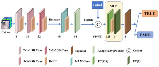
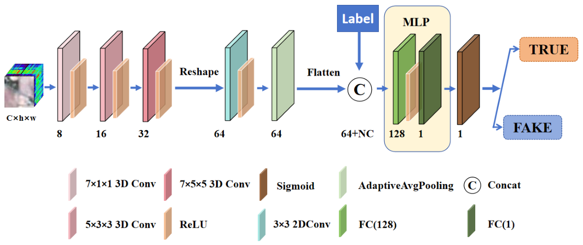
The MSCD network (Figure 4), inspired by the conditional discriminator in 3D-HyperGAMO [34], combines multiscale spectral–spatial convolutions with an MLP-based conditional head to distinguish real HSI patches from class-conditioned synthetic patches generated by AGINR. It uses three 3D convolution layers with kernel sizes of , , and , followed by a 2D convolution and global average pooling for compact feature representation. This design enlarges the receptive field and captures complementary multiscale spectral–spatial cues with modest cost. The pooled feature is concatenated with the class-condition vector and fed into a two-layer MLP followed by a sigmoid function, producing a bounded adversarial score . This output is not interpreted as a calibrated posterior probability. Instead, the sigmoid function constrains the score range, while the discriminator is optimized by enlarging the score gap between real and synthesized class-conditioned patches. During adversarial training, MSCD provides gradients that constrain generated patches relative to real training patches of the corresponding class, while target-class consistency is imposed separately by HCT.
Figure 4.
The structure of Multiscale Conditional Discriminator Network.
2.4. Hybrid CNN-Transformer Classifier Network
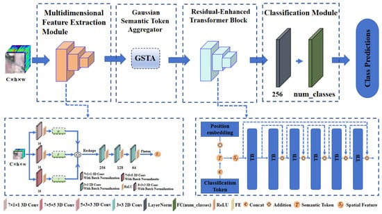
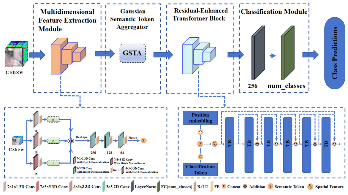
The proposed Hybrid CNN–Transformer (HCT) classifier (Figure 5) learns discriminative and robust spectral–spatial representations for HSI patch classification under severe class imbalance. Unlike a vanilla “CNN + Transformer” pipeline, it combines convolutional encoding for local spectral–spatial feature extraction with token-based global modeling for long-range semantic dependencies. It is composed of four parts: (1) a Multidimensional Feature Encoding (MFE) module for spectral–spatial encoding and adaptive fusion, (2) a Gaussian Semantic Token Aggregator (GSTA) for semantic token aggregation from dense feature maps, (3) a Residual-Enhanced Transformer Block (RETB) for global dependency modeling, and (4) a lightweight classification head. To reduce majority-class bias, HCT is trained with both real HSI patches and AGINR-synthesized minority patches, improving class balance and minority-class recognition when labeled samples are scarce.
Figure 5.
The structure of Hybrid CNN–Transformer Classifier Network.
2.4.1. Multidimensional Feature Encoding Module
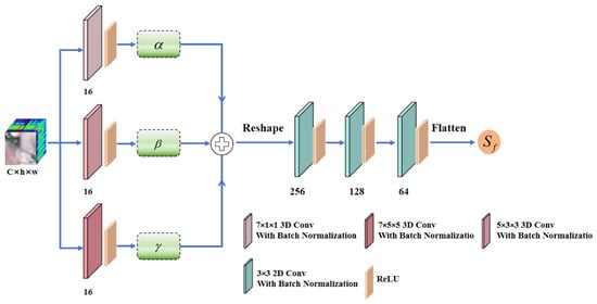
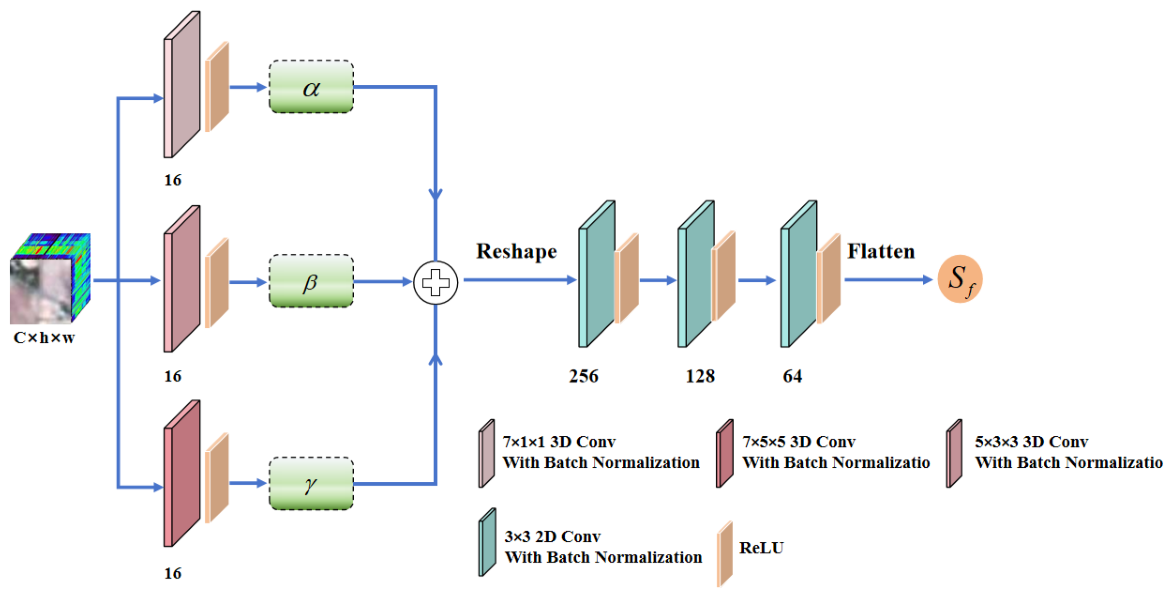
The MFE module (Figure 6) extracts joint spectral–spatial features from real and generated HSI patches through a shallow multi-branch 3D–2D hybrid encoder. Instead of using a fixed single-stream receptive field, MFE employs learnable branch reweighting to adaptively emphasize informative features. Its front-end three-branch parallel 3D convolutional block (TP3D-CB) uses , , and convolution branches for spectral feature extraction, local spatial pattern modeling, and joint spectral–spatial dependency learning, respectively.
Figure 6.
The structure of MFE.
Each branch is followed by Batch Normalization and GELU. The three branch outputs are fused by globally shared learnable branch weights for reweighted multiscale aggregation, similar to the generator AMFE module. The fused 3D features are flattened along the spectral dimension into 2D feature maps and refined by a three-layer 2D convolutional block (2D-CB) with BN and ReLU. The refined 2D features are finally flattened into , where N is the number of spatial positions and .
2.4.2. Gaussian Semantic Token Aggregator
To reduce spatial feature redundancy, we propose a Gaussian Semantic Token Aggregator (GSTA). Unlike conventional CNN–Transformer pipelines that directly flatten spatial features or use simple global pooling, GSTA extracts a compact set of semantic tokens from the flattened spatial feature sequence to improve modeling efficiency and cross-spatial semantic aggregation. It aggregates spatial features into L semantic tokens, denoted as , computed as follows:
In the above formulation, denotes the spatial feature sequence extracted from MFE. is a learnable weighting matrix for attention-score computation, initialized from a Gaussian distribution , with a mean of 0 and a standard deviation of 0.02. Softmax is applied along the spatial dimension N to produce token-wise attention weights . The learnable projection matrix maps spatial features to value vectors . The semantic token sequence is then obtained by aggregating V with A, yielding a semantic-aware low-redundancy representation for subsequent Transformer-based spectral–spatial modeling.
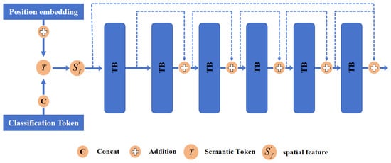
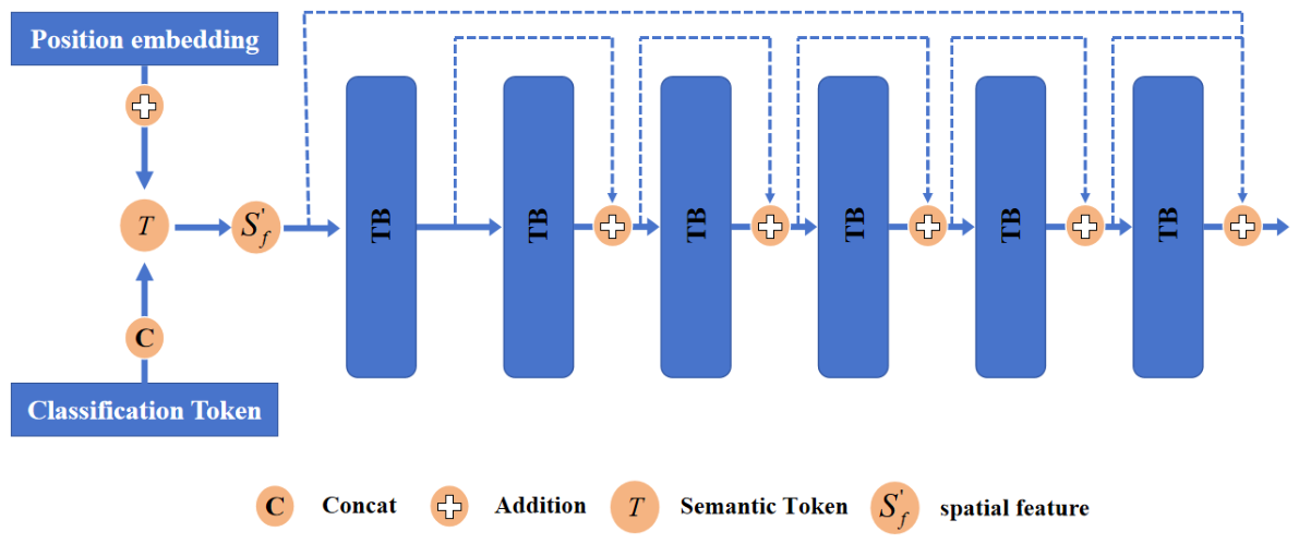
2.4.3. Residual-Enhanced Transformer Block
To model the high-level semantic dependencies in the semantic tokens aggregated by GSTA, we propose a RETB (Figure 7) to learn discriminative semantic representations for accurate classification. Unlike a vanilla stacked Transformer with only intra-block residuals, RETB introduces cross-layer residual links between successive Transformer Blocks and an outer global residual path from the input tokens to the final output. It consists of six stacked Transformer Blocks with inter-block and global residual connections. This design captures global dependencies while preserving local spatial details, thereby improving network performance. The output is computed as follows:
Figure 7.
The structure of RETB. Solid arrows indicate the main feature-propagation path, while dashed arrows denote the cross-layer and global residual connections.
Here, denotes the discriminative semantic features extracted by RETB, and denote the outputs of its six Transformer layers. is constructed by prepending a learnable classification token (CT) to the semantic tokens from GSTA and adding a shared learnable position embedding (PE) to all tokens. The resulting sequence is fed into RETB for deep feature extraction. This design allows the CT to interact with local tokens for global semantic extraction and global context aggregation, while PE enhances spatial awareness and improves feature completeness and discriminability. Finally, the final-layer hidden representation of the CT is normalized by LayerNorm and passed through a fully connected layer to produce the U-way class logits.
2.4.4. Loss Function
The overall training objective consists of three components: classifier supervision, conditional bounded-score adversarial learning with gradient-norm regularization, and class-consistency regularization. Let be a real HSI patch with class index and one-hot class condition , and denotes a synthesized patch. The discriminator outputs a sigmoid-bounded adversarial score, while the classifier produces U-way class logits. denotes the cross-entropy loss and the stop-gradient operator.
Classifier Supervision
The classifier is trained using both real and synthesized minority-class patches, where gradients from synthesized samples are blocked from flowing into the generator:
No additional weighting coefficient is introduced between the real-sample and synthesized-sample classification losses in Equation (13); both terms are assigned equal unit weights.
Conditional Bounded-Score Adversarial Learning
To distinguish real and synthesized patches under class conditioning while maintaining a controlled discriminator output range, we adopt a conditional bounded-score adversarial objective:
The discriminator minimizes to assign higher bounded adversarial scores to real patches and lower scores to synthesized patches. To stabilize adversarial optimization in the high-dimensional spectral–spatial space, an interpolation-based gradient-norm regularization term is introduced. This regularization is inspired by gradient-penalized adversarial learning [35], and its strength is controlled by the hyperparameter . The gradient-norm regularization coefficient is set to in all experiments.
where . The regularization encourages the discriminator input-gradient norm along the interpolation paths between real and synthesized patches to remain close to one, thereby avoiding excessively large or vanishing gradients. Since the discriminator retains a sigmoid-bounded output, the proposed objective is not intended to estimate the Wasserstein-1 distance and therefore differs from the standard WGAN-GP formulation.
Generator Objective with Class-Consistency
The generator is trained to increase the discriminator scores of synthesized patches while enforcing class consistency:
In Equation (16), unit coefficients are used for both the adversarial and class-consistency terms. In practice, the discriminator is updated multiple times per generator update. During generator optimization, the classifier is fixed and does not receive gradients from the class-consistency term.
2.5. Evaluation Scope of Synthetic Augmentation
During joint optimization, the generated patches are constrained by both class-conditional adversarial supervision and classifier-based class-consistency regularization. The former encourages compatibility with real training patches from the corresponding minority class, whereas the latter promotes target-class discriminability.
Since PCA is applied before patch extraction, the generated patches are primarily designed as task-oriented augmentation samples rather than physical reconstructions of the original reflectance spectra. Their effectiveness is therefore evaluated through downstream classification performance, including minority-class recognition, OA, AA, , class-wise accuracy, and controlled ablation studies.
3. Results
3.1. Datasets
We validate 3D-GIGAMO on four real-world HSI benchmarks, including Indian Pines (IP), Pavia University (UP), WHU-Hi-LongKou (LK), and Salinas (SA), to examine its classification performance.
3.1.1. Indian Pines Dataset
AVIRIS captured the Indian Pines scene in northwest Indiana, USA, in 1992. It originally comprised 224 bands across 0.4–2.5 m, with pixels and 20 m spatial resolution. The scene contains 16 land-cover classes. For experiments, we excluded 24 bands affected by noise or water absorption, retaining 200 bands.
3.1.2. Pavia University Dataset
ROSIS captured the Pavia University scene in northern Italy in 2001. The raw image contained 115 spectral bands across 0.43–0.86 m, with a size of pixels, 1.3 m spatial resolution, and nine land-cover categories. Excluding 12 noise-affected bands left 103 bands for experiments.
3.1.3. WHU-Hi-LongKou Dataset
Wuhan University collected the WHU-Hi-LongKou scene in 2019 over Longkou Town, Hubei, China, using a UAV-mounted Headwall Nano-Hyperspec sensor (Headwall Photonics, Inc., Bolton, MA, USA). The dataset comprises 270 bands within 0.4–1.0 m, pixels, approximately 0.463 m spatial resolution, and nine agricultural/artificial classes.
3.1.4. Salinas Dataset
AVIRIS acquired the Salinas scene in California’s Salinas Valley, USA. The dataset contains 224 bands spanning 0.4–2.5 m and has pixels, a 3.7 m ground sampling distance, and 16 land-cover classes dominated by vegetables, bare soil, and vineyards. After discarding 20 water-absorption bands, 204 bands were used.
Table 1, Table 2, Table 3 and Table 4 report the class labels and train/test sample distributions of the four benchmark datasets. For IP, UP, LK, and SA, the training sets are constructed by randomly selecting 10%, 1%, 0.2%, and 1% of labeled samples from each class, respectively. Considering the substantial differences in the total numbers of labeled samples among the four datasets, dataset-specific training ratios are adopted to maintain a limited-label evaluation setting while avoiding the use of an excessively large number of training samples for the larger datasets.
Table 1.
Training and test sample allocation for each class in the IP dataset.
Table 2.
Training and test sample allocation for each class in the UP dataset.
Table 3.
Training and test sample allocation for each class in the LK dataset.
Table 4.
Training and test sample allocation for each class in the SA dataset.
3.2. Experimental Settings
Experiments were run in PyTorch 2.4.0 on one NVIDIA GeForce RTX A5000 GPU with 24 GB memory. 3D-GIGAMO was trained with AdamW for 1500 epochs using a batch size of 64. The learning rates were for IP, UP, and SA and for LK. Patch sizes were 11, 15, 15, and 15 for IP, UP, LK, and SA, respectively. PCA [36] reduced the spectral dimension of each dataset to 30. The gradient-norm regularization coefficient was set to in all experiments. During adversarial training, the discriminator was updated five times for each generator update, corresponding to a discriminator-to-generator update ratio of 5:1.
3.3. Experimental Results and Analysis
To evaluate 3D-GIGAMO for class-imbalanced hyperspectral image classification, it is benchmarked against several representative competitive approaches, including general HSI classification models and imbalance-aware methods. The compared general HSI classification methods include GAHT [37], MorphFormer [38], GraphGST [39], DSFormer [40], and S2Mamba [18]. In addition, E-SPPO [25] and ADA-Es-gcForest [27] are included as representative imbalance-aware baselines. E-SPPO combines synthetic minority oversampling with pixel-pair-based data augmentation to address class imbalance and limited training samples, while ADA-Es-gcForest integrates ADASYN-based minority oversampling with a forest classifier to improve minority-class recognition.
Table 5, Table 6, Table 7 and Table 8 present the OA, AA, and values obtained on the four benchmark datasets. AA is particularly important for class-imbalanced classification because it reflects average recognition across classes and is less dominated by majority classes than OA. The numerical results and classification maps are further examined to highlight the effectiveness of the proposed method in overall accuracy, minority-class recognition, and class-balanced performance.
Table 5.
Performance comparison of competing methods on the IP test set using OA (%)/AA (%)/. The top scores are highlighted in bold.
Table 6.
Performance comparison of competing methods on the UP test set using OA (%)/AA (%)/. The top scores are highlighted in bold.
Table 7.
Performance comparison of competing methods on the LK test set using OA (%)/AA (%)/. The top scores are highlighted in bold.
Table 8.
Performance comparison of competing methods on the SA test set using OA (%)/AA (%)/. The top scores are highlighted in bold.
3.3.1. Indian Pines
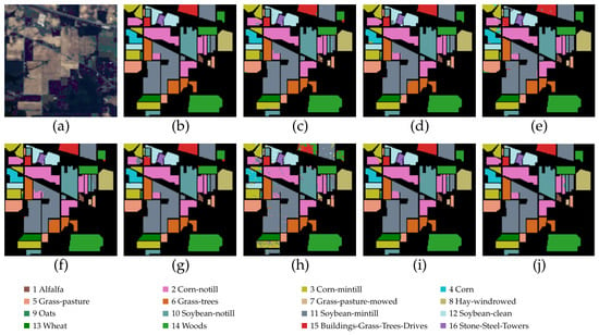
Table 5 shows that on the IP dataset, 3D-GIGAMO achieves the best OA, AA, and , reaching 99.37%, 99.58%, and 0.9928, respectively. In addition, 3D-GIGAMO attains the highest or tied-highest accuracy in 12 of the 16 categories, demonstrating strong class-wise discriminative capability. Compared with the two imbalance-aware baselines, E-SPPO and ADA-Es-gcForest, 3D-GIGAMO achieves higher OA, AA, and , indicating that the proposed generation–classification framework can effectively improve class-balanced HSI classification under imbalanced training conditions. These advantages are also supported by the prediction maps in Figure 8, which show more accurate results for most categories.
Figure 8.
Classification maps comparison for the IP dataset. (a) False-color map. (b) Ground truth. (c) GAHT. (d) MorphFormer. (e) GraphGST. (f) DSFormer. (g) S2Mamba. (h) E-SPPO. (i) ADA-Es-gcForest. (j) Proposed.
3.3.2. Pavia University
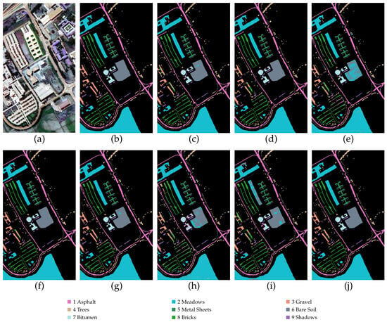
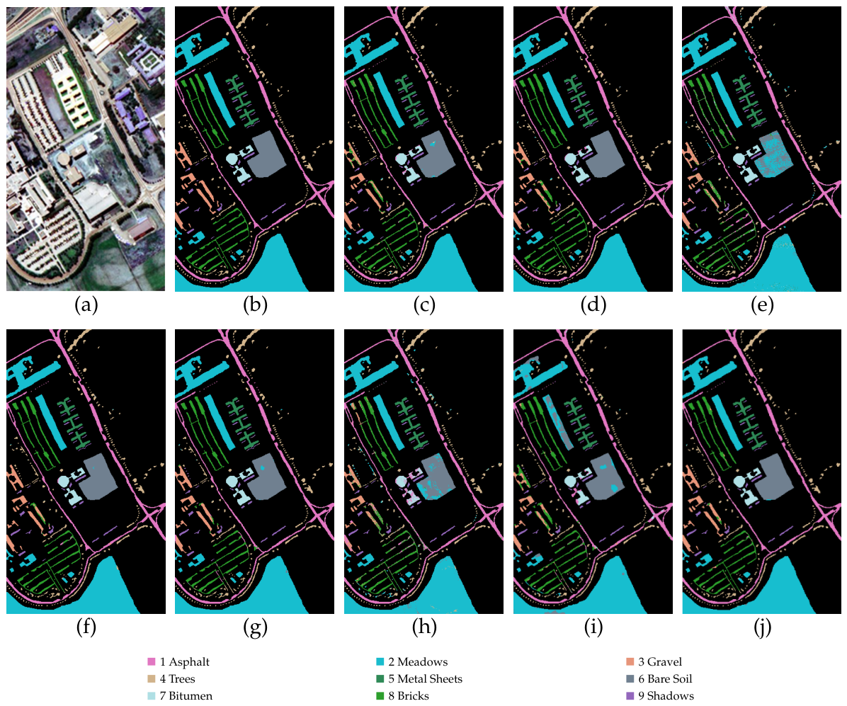
Table 6 reports the classification results on the UP dataset. 3D-GIGAMO achieves an OA of 99.13%, an AA of 98.45%, and a of 0.9885, yielding the best overall performance among the compared methods. More importantly, its class-wise accuracies remain consistently high, with the lowest category accuracy reaching 96.15%. This relatively high performance floor indicates that the proposed method maintains stable recognition even for more difficult categories. Compared with E-SPPO and ADA-Es-gcForest, 3D-GIGAMO also achieves higher overall evaluation metrics, further demonstrating its effectiveness under imbalanced training conditions. Figure 9 presents the corresponding classification maps.
Figure 9.
Classification maps comparison for the UP dataset. (a) False-color map. (b) Ground truth. (c) GAHT. (d) MorphFormer. (e) GraphGST. (f) DSFormer. (g) S2Mamba. (h) E-SPPO. (i) ADA-Es-gcForest. (j) Proposed.
3.3.3. WHU-Hi-LongKou
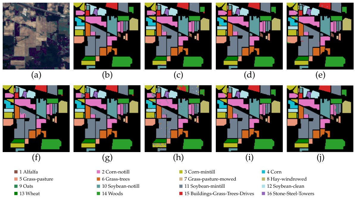
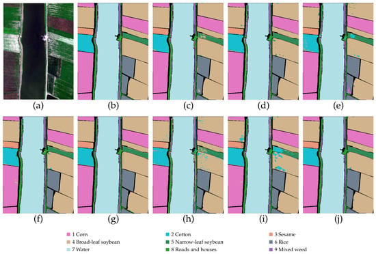
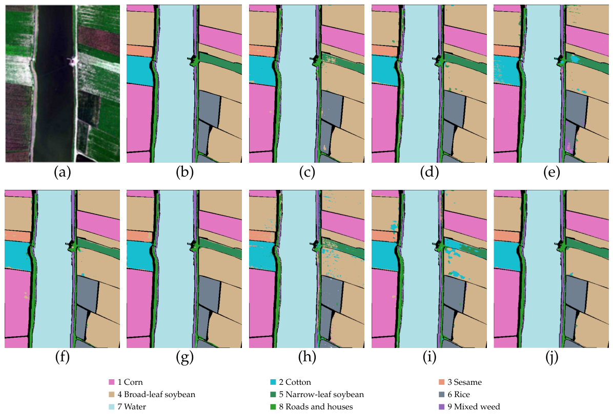
According to Table 7, on the LK dataset, 3D-GIGAMO achieved the best OA, AA, and , reaching 98.86%, 96.88%, and 0.9851, respectively. In particular, the accuracy of Narrow-leaf soybean increases markedly to 96.67%, highlighting the capability of the proposed method in recognizing minority and difficult classes. Figure 10 also shows more accurate and spatially coherent classification results in complex scenes.
Figure 10.
Classification maps comparison for the LK dataset. (a) False-color map. (b) Ground truth. (c) GAHT. (d) MorphFormer. (e) GraphGST. (f) DSFormer. (g) S2Mamba. (h) E-SPPO. (i) ADA-Es-gcForest. (j) Proposed.
3.3.4. Salinas
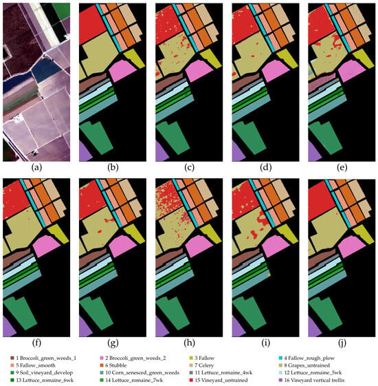
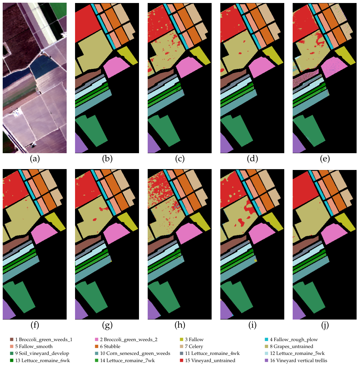
As shown in Table 8, 3D-GIGAMO achieves the highest OA, AA, and , showing strong robustness under class-imbalanced conditions. It obtains the highest or tied-highest accuracy in 12 of the 16 categories, with 7 categories reaching 100%, which further demonstrates its strong discriminative capability across diverse land-cover classes. Figure 11 shows that 3D-GIGAMO produces more precise boundary delineations, especially for challenging classes such as Broccoli_green_weeds_1 (brown), Fallow_smooth (light orange), and Lettuce_romaine_7wk (light green).
Figure 11.
Classification maps comparison for the SA dataset. (a) False-color map. (b) Ground truth. (c) GAHT. (d) MorphFormer. (e) GraphGST. (f) DSFormer. (g) S2Mamba. (h) E-SPPO. (i) ADA-Es-gcForest. (j) Proposed.
3.4. Computational Complexity and Inference Efficiency
To evaluate the computational overhead of the proposed method, we compare its parameter count, FLOPs, full-map inference time, and peak GPU memory with those of 3D-CNN, DSFormer, and S2Mamba. All models are evaluated on the UP dataset using the same NVIDIA GeForce RTX A5000 GPU. The input contains 30 PCA components with a spatial size of , consistent with the experimental settings. FLOPs are calculated for processing a single input patch, whereas the full-map inference time measures the time required to generate the corresponding classification map. For 3D-GIGAMO, all complexity metrics reported in Table 9 correspond to the HCT classifier used during inference, rather than to the complete AGINR–MSCD–HCT training framework.
Table 9.
Computational complexity and inference efficiency on the UP dataset. FLOPs are measured for one input patch, while full-map time represents the inference time for generating the classification map.
During inference, AGINR and MSCD are no longer used, and only the HCT classifier is retained for test-sample prediction. The complete training framework, including AGINR, MSCD, and HCT, contains 49.094 million parameters. As shown in Table 9, HCT contains 1.785 million parameters and requires 68.836 MFLOPs for one input patch. Its full-map inference time and peak GPU memory consumption are 42.41 s and 177.44 MB, respectively. Although HCT introduces higher computational cost than the lightweight 3D-CNN and S2Mamba models, it requires substantially fewer FLOPs, shorter inference time, and less GPU memory than DSFormer. Combined with the classification results in Table 6, these results indicate that 3D-GIGAMO achieves a reasonable trade-off between classification performance and inference efficiency.
4. Discussion
4.1. Ablation Study
To evaluate the role of individual modules in 3D-GIGAMO, six ablation studies are carried out on the UP dataset. In each experiment, one module is removed, while the rest of the architecture and training strategies remain identical to those of the full model for controlled comparison. These ablations evaluate the contribution of the generated patches and the key components to classification performance. In particular, removing GGM tests the contribution of real-patch guidance, while replacing IGM with random noise evaluates the benefit of coordinate-based generation. The results are reported in Table 10.
Table 10.
Ablation results for different modules of 3D-GIGAMO. The best results are highlighted in bold.
4.1.1. Ablation of the GGM
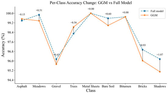
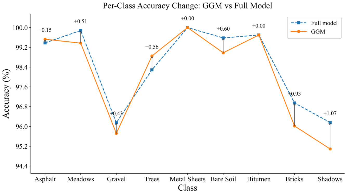
Excluding GGM decreases OA from 99.13% to 98.77% and AA from 98.45% to 98.13% for the UP dataset. According to Figure 12, the complete model obtains superior results in most categories, especially Shadows, Bricks, and Bare Soil. These results indicate that real-sample guidance helps improve minority-class representation and discrimination.
Figure 12.
Per-class accuracy comparison on the UP dataset for the full model and its GGM-removed counterpart.
4.1.2. Ablation of the Generator’s IGM
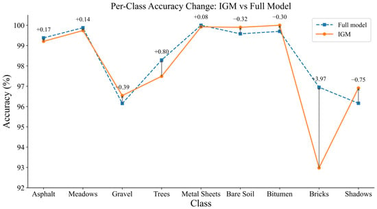
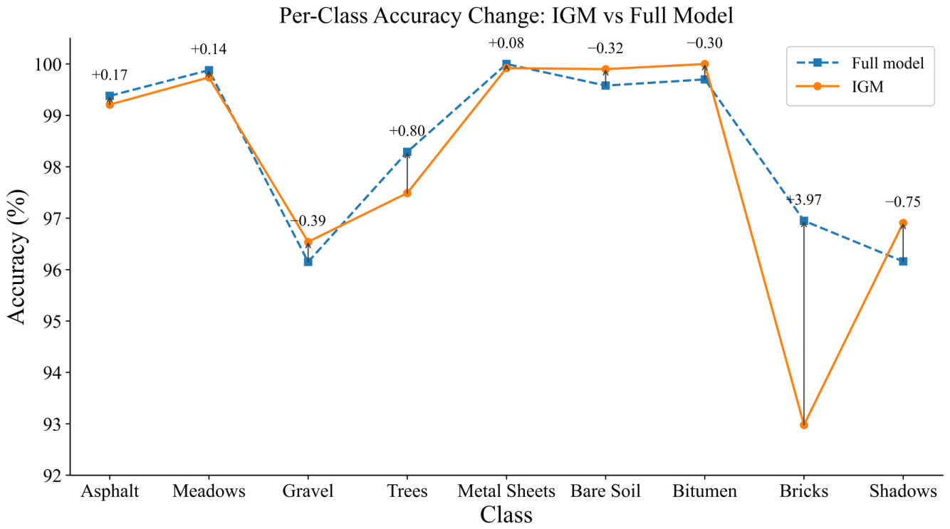
Replacing IGM with random noise reduces OA to 98.72% and AA to 98.07%. Figure 13 illustrates that the complete model shows superior category-wise results, with the largest gain observed for Bricks. This finding indicates that coordinate-based implicit representation offers stronger minority-class oversampling capability than noise-driven generation.
Figure 13.
Per-class accuracy comparison on the UP dataset for the full model and its IGM-removed counterpart.
4.1.3. Ablation of the GSTA
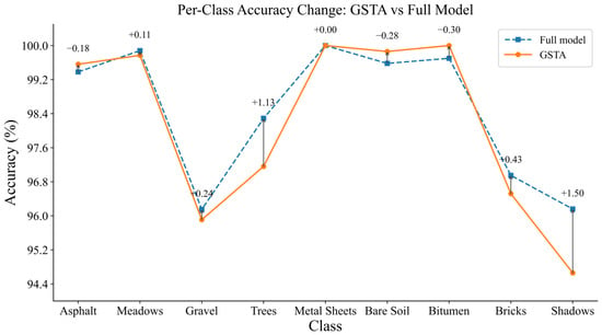
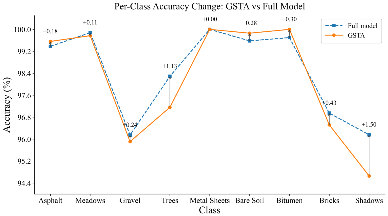
Removing GSTA causes a slight performance drop, with OA decreasing to 98.99% and AA to 98.16%. As shown in Figure 14, the class-wise differences are generally small, but the full model is more stable across categories. This suggests that GSTA mainly serves as a lightweight regularizer that reduces redundancy and stabilizes token formation.
Figure 14.
Per-class accuracy comparison on the UP dataset for the full model and its GSTA-removed counterpart.
4.1.4. Ablation of the RETB
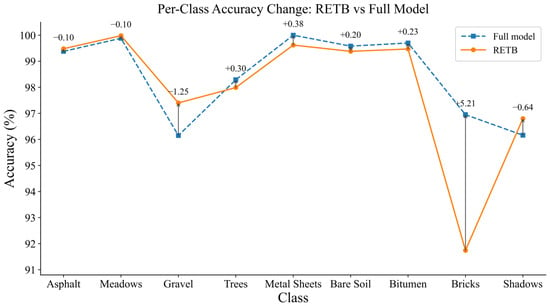
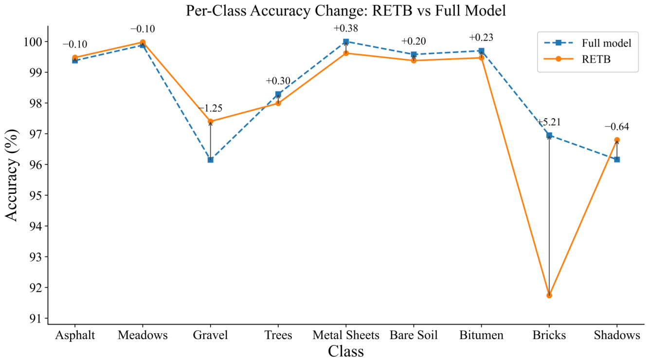
Without RETB, OA and AA drop to 98.73% and 98.12%, respectively. Figure 15 shows that Bricks is particularly affected by the removal of RETB, indicating the benefit of global contextual modeling. These results confirm that RETB improves both discriminability and class-wise stability.
Figure 15.
Per-class accuracy comparison on the UP dataset for the full model and its RETB-removed counterpart.
4.1.5. Ablation of the TP3D-CB
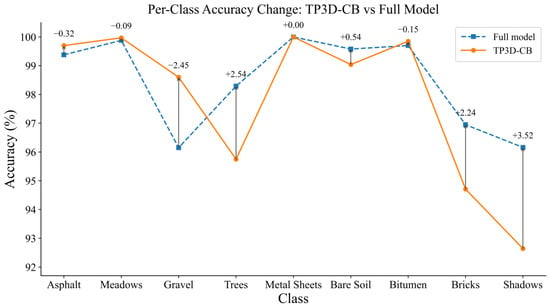
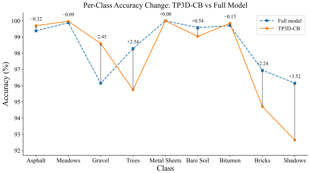
Removing TP3D-CB reduces OA from 99.13% to 98.75% and AA from 98.45% to 97.98%. As shown in Figure 16, the most noticeable accuracy degradations occur for Shadows, Trees, and Bricks. This highlights the necessity of modeling spectral information for effective spectral–spatial feature extraction.
Figure 16.
Per-class accuracy comparison on the UP dataset for the full model and its TP3D-CB-removed counterpart.
4.1.6. Ablation of the 2D-CB
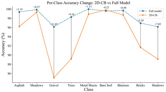
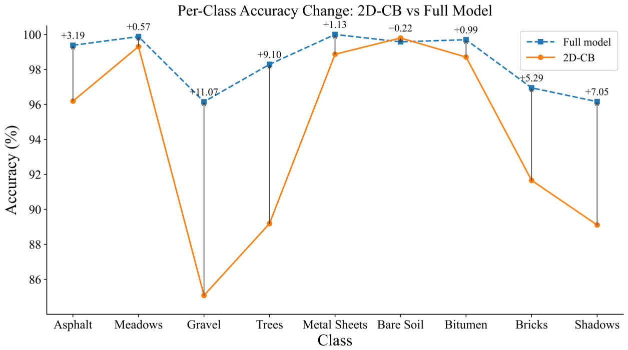
Removing 2D-CB leads to the largest performance degradation, with OA and AA dropping to 96.54% and 94.21%, respectively. Figure 17 further shows clear declines in most categories, especially Gravel, Trees, Shadows, and Bricks. Therefore, 2D-CB is essential for preserving spatial detail and providing the classifier with strong basic discriminative capability.
Figure 17.
Per-class accuracy comparison on the UP dataset for the full model and its 2D-CB-removed counterpart.
Overall, the ablation results show that the components of 3D-GIGAMO contribute in complementary ways. Among all components, 2D-CB produces the largest performance gain, while IGM, GGM, GSTA, RETB, and TP3D-CB provide complementary improvements in class-balanced recognition. A synthesis of Table 10 and Figure 12, Figure 13, Figure 14, Figure 15, Figure 16 and Figure 17 shows that the 2D-CB is the core spatial feature extractor and provides the classifier’s basic discriminative capability; removing it causes the largest drop in OA and AA. In contrast, the proposed modules mainly target class imbalance and prediction stability. The IGM and GGM provide coordinate-based, real-guided synthetic augmentation, and their removal reduces OA and AA, indicating that the resulting task-oriented patches contribute to minority-class discrimination. TP3D-CB and RETB strengthen spectral–spatial coupling and global contextual representation, while GSTA supports token formation and stabilizes class-wise predictions. These ablations demonstrate the contribution of the generated patches and the proposed modules to class-balanced classification.
4.2. Sensitivity Analysis
4.2.1. Sensitivity to the Gradient-Norm Regularization Coefficient
To investigate the influence of the gradient-norm regularization coefficient, we evaluate on the Indian Pines dataset while keeping all other experimental settings unchanged. As shown in Table 11, achieves the best classification performance, with an OA of 99.37%, an AA of 99.58%, and a of 0.9928.
Table 11.
Sensitivity analysis of the gradient-norm regularization coefficient on the Indian Pines dataset. The best results are highlighted in bold.
4.2.2. Sensitivity to the Training Sample Ratio
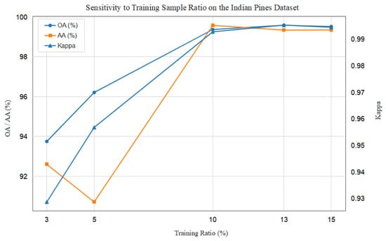
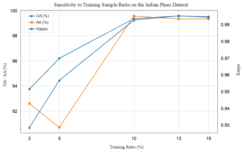
To assess the sensitivity of 3D-GIGAMO to label availability, we conduct additional experiments on the Indian Pines dataset using training ratios of 3%, 5%, 10%, 13%, and 15%, while keeping all other experimental settings unchanged. As shown in Figure 18, OA and increase from 93.75% and 0.9287 at 3% to 99.37% and 0.9928 at 10%, respectively. Although AA decreases slightly from 92.60% at 3% to 90.71% at 5%, it subsequently increases to 99.58% at 10%. When the training ratio is further increased to 13% and 15%, OA, AA, and remain consistently high with only minor variations. These results show that increasing the labeled proportion generally improves classification performance, while the performance tends to stabilize once the training ratio reaches 10%.
Figure 18.
Sensitivity to different training sample ratios on the Indian Pines dataset.
5. Conclusions
This study tackles HSI class imbalance, which often causes classifiers to bias toward majority classes. We propose 3D-GIGAMO as a task-oriented generative oversampling framework that integrates GINR with adversarial learning. GINR performs conditional oversampling for minority classes in a continuous coordinate space, where real training patches provide guidance for the generation process. Transformer encoding and AMFE enrich global contextual modeling and multiscale semantic representation. A conditional discriminator and a bounded-score adversarial objective with gradient-norm regularization stabilize adversarial learning, while HCT supplies target-class consistency constraints.
Results on four public benchmark datasets show that 3D-GIGAMO consistently obtains higher OA, AA, and than several representative methods, including the imbalance-aware baseline ADA-Es-gcForest. Ablation results further verify the complementary contributions of the key modules, with TP3D-CB, IGM, RETB, and 2D-CB showing notable effects on different aspects of the classification performance. Overall, the proposed joint augmentation–classification framework effectively alleviates class imbalance and improves class-balanced HSI classification performance. Nevertheless, the generator is optimized primarily for task-specific discriminability. Evaluating the spectral fidelity and distributional diversity of the generated samples remains an important direction for future work.
Author Contributions
Conceptualization, Z.W.; methodology, Z.W.; validation, Z.M. and M.Y.; formal analysis, X.Z. and Y.Z.; investigation, X.W.; resources, L.M.; data curation, X.D.; writing—original draft preparation, Z.W.; writing—review and editing, Z.M. and M.Y.; visualization, L.M.; supervision, Z.M. and M.Y.; project administration, Z.M.; funding acquisition, Z.M. All authors have read and agreed to the published version of the manuscript.
Funding
This research was funded by the National Key Research and Development Program of China, grant number 2021YFA0715104; the National Natural Science Foundation of China, grant number 42071309; and the FDCT-supported Open Project of the State Key Laboratory of Lunar and Planetary Sciences, Macau University of Science and Technology, grant number 002/2024/SKL.
Data Availability Statement
Data will be made available upon request, and the code will be provided shortly. https://github.com/zhiweiw-23/3D-GIGAMO (accessed on 23 September 2026).
Conflicts of Interest
The authors declare no conflicts of interest.
References
- Zhu, C.; Song, X.; Li, Y.; Deng, S.; Zhang, T. A spatial-frequency dual-domain implicit guidance method for hyperspectral and multispectral remote sensing image fusion based on Kolmogorov–Arnold network. Inf. Fusion 2025, 123, 103261. [Google Scholar] [CrossRef] [Scilit]
- Zhu, C.; Deng, S.; Song, X.; Li, Y.; Wang, Q. Mamba collaborative implicit neural representation for hyperspectral and multispectral remote sensing image fusion. IEEE Trans. Geosci. Remote Sens. 2025, 63, 5504915. [Google Scholar] [CrossRef] [Scilit]
- Bioucas-Dias, J.M.; Plaza, A.; Camps-Valls, G.; Scheunders, P.; Nasrabadi, N.; Chanussot, J. Hyperspectral remote sensing data analysis and future challenges. IEEE Geosci. Remote Sens. Mag. 2013, 1, 6–36. [Google Scholar] [CrossRef] [Scilit]
- Moharram, M.A.; Sundaram, D.M. Land use and land cover classification with hyperspectral data: A comprehensive review of methods, challenges and future directions. Neurocomputing 2023, 536, 90–113. [Google Scholar] [CrossRef] [Scilit]
- Biau, G. Analysis of a random forests model. J. Mach. Learn. Res. 2012, 13, 1063–1095. [Google Scholar]
- Ham, J.; Chen, Y.; Crawford, M.M.; Ghosh, J. Investigation of the Random Forest Framework for Classification of Hyperspectral Data. IEEE Trans. Geosci. Remote Sens. 2005, 43, 492–501. [Google Scholar] [CrossRef] [Scilit]
- Ohsaki, M.; Wang, P.; Matsuda, K.; Katagiri, S.; Watanabe, H.; Ralescu, A. Confusion-matrix-based kernel logistic regression for imbalanced data classification. IEEE Trans. Knowl. Data Eng. 2017, 29, 1806–1819. [Google Scholar] [CrossRef] [Scilit]
- Chen, Y.; Lin, Z.; Zhao, X.; Wang, G.; Gu, Y. Deep learning-based classification of hyperspectral data. IEEE J. Sel. Top. Appl. Earth Obs. Remote Sens. 2014, 7, 2094–2107. [Google Scholar] [CrossRef] [Scilit]
- Yu, S.; Jia, S.; Xu, C. Convolutional neural networks for hyperspectral image classification. Neurocomputing 2017, 219, 88–98. [Google Scholar] [CrossRef] [Scilit]
- Zhong, Z.; Li, J. Hyperspectral image classification using deep convolutional neural networks. J. Comput. Vis. Imaging Syst. 2017, 3. [Google Scholar] [CrossRef] [Scilit]
- Gao, Q.; Lim, S.; Jia, X. Hyperspectral image classification using convolutional neural networks and multiple feature learning. Remote Sens. 2018, 10, 299. [Google Scholar] [CrossRef] [Scilit]
- Makantasis, K.; Karantzalos, K.; Doulamis, A.; Doulamis, N. Deep supervised learning for hyperspectral data classification through convolutional neural networks. In IEEE International Geoscience and Remote Sensing Symposium (IGARSS); IEEE: Piscataway, NJ, USA, 2015; pp. 4959–4962. [Google Scholar] [CrossRef] [Scilit]
- Hamida, A.B.; Benoit, A.; Lambert, P.; Amar, C.B. 3-D deep learning approach for remote sensing image classification. IEEE Trans. Geosci. Remote Sens. 2018, 56, 4420–4434. [Google Scholar] [CrossRef] [Scilit]
- Zhai, H.; Zhao, J. Two-stream spectral-spatial convolutional capsule network for hyperspectral image classification. Int. J. Appl. Earth Obs. Geoinf. 2024, 127, 103614. [Google Scholar] [CrossRef] [Scilit]
- Jiang, Y.; Zhang, Z.; Zhang, C.; Zhou, H.; Ma, Q.; Zhong, C. S2WaveNet: A novel spectral–spatial wave network for hyperspectral image classification. Int. J. Appl. Earth Obs. Geoinf. 2024, 128, 103754. [Google Scholar] [CrossRef] [Scilit]
- Zhang, Z.; Zhou, H.; Zhang, C.; Zhang, X.; Jiang, Y. A multi-level deformable gated aggregated network for hyperspectral image classification. Int. J. Appl. Earth Obs. Geoinf. 2023, 123, 103482. [Google Scholar] [CrossRef] [Scilit]
- Wang, C.; Huang, J.; Lv, M.; Du, H.; Wu, Y.; Qin, R. A local enhanced Mamba network for hyperspectral image classification. Int. J. Appl. Earth Obs. Geoinf. 2024, 133, 104092. [Google Scholar] [CrossRef] [Scilit]
- Wang, G.; Zhang, X.; Peng, Z.; Zhang, T.; Jiao, L. S2Mamba: A spatial–spectral state space model for hyperspectral image classification. IEEE Trans. Geosci. Remote Sens. 2025, 63, 5511413. [Google Scholar] [CrossRef] [Scilit]
- Wang, D.; Zhuang, L.; Gao, L.; Sun, X.; Zhao, X.; Plaza, A. Sliding Dual-Window-Inspired Reconstruction Network for Hyperspectral Anomaly Detection. IEEE Trans. Geosci. Remote Sens. 2024, 62, 5504115. [Google Scholar] [CrossRef] [Scilit]
- Wang, D.; Ren, L.; Sun, X.; Gao, L.; Chanussot, J. Nonlocal and Local Feature-Coupled Self-Supervised Network for Hyperspectral Anomaly Detection. IEEE J. Sel. Top. Appl. Earth Obs. Remote Sens. 2025, 18, 6981–6993. [Google Scholar] [CrossRef] [Scilit]
- Zhang, H.; Sun, H.; Sun, X.; Gao, H.; Yu, H.; Zhang, B. SPG-OD: Spectral-Prior-Guided Object Detection for Hyperspectral Remote Sensing Images. IEEE Trans. Geosci. Remote Sens. 2026, 64, 5523115. [Google Scholar] [CrossRef] [Scilit]
- Zhang, H.; Sun, H.; Gao, H.; Gao, L.; Zhang, B. Hyperspectral Remote Sensing Object Detection via Cross-Domain Learning From Visible Images. IEEE Trans. Geosci. Remote Sens. 2026, 64, 5510518. [Google Scholar] [CrossRef] [Scilit]
- Paoletti, M.E.; Mogollon-Gutierrez, O.; Moreno-Álvarez, S.; Sancho, J.C.; Haut, J.M. A Comprehensive Survey of Imbalance Correction Techniques for Hyperspectral Data Classification. IEEE J. Sel. Top. Appl. Earth Obs. Remote Sens. 2023, 16, 5297–5314. [Google Scholar] [CrossRef] [Scilit]
- Galar, M.; Fernández, A.; Barrenechea, E.; Herrera, F. EUSBoost: Enhancing ensembles for highly imbalanced data-sets by evolutionary undersampling. Pattern Recognit. 2013, 46, 3460–3471. [Google Scholar] [CrossRef] [Scilit]
- Feng, W.; Long, Y.; Dauphin, G.; Quan, Y.; Huang, W.; Xing, M. Ensemble synthetic oversampling with pixel pair for class-imbalanced and small-sized hyperspectral data classification. Int. J. Appl. Earth Obs. Geoinf. 2024, 128, 103697. [Google Scholar] [CrossRef] [Scilit]
- Ramentol, E.; Caballero, Y.; Bello, R.; Herrera, F. SMOTE-RSB*: A hybrid preprocessing approach based on oversampling and undersampling for high imbalanced data-sets using SMOTE and rough sets theory. Knowl. Inf. Syst. 2012, 33, 245–265. [Google Scholar] [CrossRef] [Scilit]
- Datta, D.; Mallick, P.K.; Reddy, A.V.; Mohammed, M.A.; Jaber, M.M.; Alghawli, A.S.; Al-Qaness, M.A. A hybrid classification of imbalanced hyperspectral images using ADASYN and enhanced deep subsampled multi-grained cascaded forest. Remote Sens. 2022, 14, 4853. [Google Scholar] [CrossRef] [Scilit]
- Luo, W.; Zhang, C.; Li, Y.; Yang, F.; Zhang, D.; Hong, Z. Deeply-supervised pseudo learning with small class-imbalanced samples for hyperspectral image classification. Int. J. Appl. Earth Obs. Geoinf. 2022, 112, 102949. [Google Scholar] [CrossRef] [Scilit]
- Xu, D.; Wang, P.; Jiang, Y.; Fan, Z.; Wang, Z. Signal processing for implicit neural representations. Adv. Neural Inf. Process. Syst. 2022, 35, 13404–13418. [Google Scholar] [CrossRef] [Scilit]
- Chen, Z.; Chen, Y.; Liu, J.; Xu, X.; Goel, V.; Wang, Z.; Shi, H.; Wang, X. VideoINR: Learning video implicit neural representation for continuous space-time super-resolution. In 2022 IEEE/CVF Conference on Computer Vision and Pattern Recognition (CVPR); IEEE: Piscataway, NJ, USA, 2022; pp. 2047–2057. [Google Scholar] [CrossRef] [Scilit]
- Mildenhall, B.; Srinivasan, P.P.; Tancik, M.; Barron, J.T.; Ramamoorthi, R.; Ng, R. NeRF: Representing scenes as neural radiance fields for view synthesis. Commun. ACM 2022, 65, 99–106. [Google Scholar] [CrossRef] [Scilit]
- Jozdani, S.; Chen, D.; Pouliot, D.; Johnson, B.A. A review and meta-analysis of generative adversarial networks and their applications in remote sensing. Int. J. Appl. Earth Obs. Geoinf. 2022, 108, 102734. [Google Scholar] [CrossRef] [Scilit]
- Mullick, S.S.; Datta, S.; Das, S. Generative adversarial minority oversampling. In 2019 IEEE/CVF International Conference on Computer Vision (ICCV); IEEE: Piscataway, NJ, USA, 2019; pp. 1695–1704. [Google Scholar] [CrossRef] [Scilit]
- Roy, S.K.; Haut, J.M.; Paoletti, M.E.; Dubey, S.R.; Plaza, A. Generative adversarial minority oversampling for spectral–spatial hyperspectral image classification. IEEE Trans. Geosci. Remote Sens. 2022, 60, 5500615. [Google Scholar] [CrossRef] [Scilit]
- Gulrajani, I.; Ahmed, F.; Arjovsky, M.; Dumoulin, V.; Courville, A.C. Improved training of Wasserstein GANs. Adv. Neural Inf. Process. Syst. 2017, 30, 5769–5779. [Google Scholar]
- Prasad, S.; Bruce, L.M. Limitations of principal components analysis for hyperspectral target recognition. IEEE Geosci. Remote Sens. Lett. 2008, 5, 625–629. [Google Scholar] [CrossRef] [Scilit]
- Mei, S.; Song, C.; Ma, M.; Xu, F. Hyperspectral image classification using group-aware hierarchical transformer. IEEE Trans. Geosci. Remote Sens. 2022, 60, 5539014. [Google Scholar] [CrossRef] [Scilit]
- Roy, S.K.; Deria, A.; Shah, C.; Haut, J.M.; Du, Q.; Plaza, A. Spectral–spatial morphological attention transformer for hyperspectral image classification. IEEE Trans. Geosci. Remote Sens. 2023, 61, 5503615. [Google Scholar] [CrossRef] [Scilit]
- Jiang, M.; Su, Y.; Gao, L.; Plaza, A.; Zhao, X.L.; Sun, X.; Liu, G. GraphGST: Graph generative structure-aware transformer for hyperspectral image classification. IEEE Trans. Geosci. Remote Sens. 2024, 62, 5504016. [Google Scholar] [CrossRef] [Scilit]
- Xu, Y.; Wang, D.; Zhang, L.; Zhang, L. Dual selective fusion transformer network for hyperspectral image classification. Neural Netw. 2025, 187, 107311. [Google Scholar] [CrossRef] [Scilit]

Disclaimer/Publisher’s Note: The statements, opinions and data contained in all publications are solely those of the individual author(s) and contributor(s) and not of MDPI and/or the editor(s). MDPI and/or the editor(s) disclaim responsibility for any injury to people or property resulting from any ideas, methods, instructions or products referred to in the content. |
© 2026 by the authors. Licensee MDPI, Basel, Switzerland. This article is an open access article distributed under the terms and conditions of the Creative Commons Attribution (CC BY) license.