


Highlights
What are the main findings?
- A statistical time-series feature classification and pixel-wise TCEV modeling method was developed for SAR flood anomaly mapping.
- TFAMs provide continuous representations of flood anomalies and capture their temporal variations across different extreme flood events.
What are the implications of the main findings?
- Extreme-event characterization provides an interpretable strategy for SAR-based flood anomaly detection under complex environmental conditions.
- The proposed method enables dynamic characterization of flood anomalies beyond conventional inundation mapping.
Abstract
Flood mapping using Synthetic Aperture Radar (SAR) observations is essential for rapid disaster response, yet existing approaches often struggle to characterize rare extreme flood events due to limited temporal context and insufficient representation of flood anomalies. This study proposes a statistical time-series feature classification and pixel-wise TCEV modeling method for SAR flood anomaly mapping by integrating extreme value theory. Long-term Sentinel-1 SAR time series were used to construct nine statistical features for flood classification using a Tabular Prior-data Fitted Network (TabPFN), while a separately fitted Two-Component Extreme Value (TCEV) model was used to calculate event-period anomaly probabilities. The resulting spatial classification mask and TCEV-based anomaly probabilities were then combined to produce Temporal Flood Anomaly Maps (TFAMs). The proposed method was evaluated using four extreme flood events under diverse environmental conditions. The generated TFAMs characterized flood-related temporal anomalies, with the highest ROC-AUC 0.87 and average precision 0.81 achieved for New South Wales. The corresponding TFAM-derived binary flood extent map achieved the highest F1-score of 0.81, IoU of 0.69, and Kappa coefficient of 0.72.
1. Introduction
The increasing frequency and severity of natural disasters under global environmental change have posed substantial challenges to disaster prevention and risk management [1,2]. According to the 2025 Global Assessment Report on Disaster Risk Reduction issued by the United Nations Office for Disaster Risk Reduction, disaster risks are intensifying worldwide. Among various natural hazards, floods are among the most frequent and destructive events, causing severe impacts on human lives, infrastructure, and ecosystems [3]. Globally, floods result in hundreds of billions of dollars in economic losses annually and remain a major threat to sustainable development and societal resilience [4]. Therefore, accurate and timely flood mapping is essential for emergency response, hazard assessment, and post-disaster recovery.
Remote sensing technologies provide an effective approach for large-scale and rapid flood monitoring. In particular, Synthetic Aperture Radar (SAR) has become one of the most widely used data sources for flood mapping due to its all-weather and day-and-night imaging capabilities [5,6,7]. The open-access Sentinel-1 SAR mission, with high spatial resolution and frequent revisit capability, provides valuable observations for capturing flood dynamics over large regions [8,9,10].
The fundamental principle of SAR-based flood mapping relies on the distinct electromagnetic response of water surfaces, which generally exhibit lower backscatter intensity compared with surrounding land surfaces [11]. Existing SAR flood mapping approaches can generally be divided into single-image-based and multi-temporal methods [12]. Single-image approaches typically extract flooded areas from individual SAR acquisitions using techniques such as thresholding, texture analysis, and region-growing segmentation [13,14]. Although computationally efficient, these methods are highly sensitive to environmental conditions because certain land-cover types, including vegetated areas and wet snow, may exhibit scattering characteristics similar to water surfaces, leading to false detections and classification uncertainty [15,16]. To overcome these limitations, multi-temporal approaches exploit backscatter variations between pre-flood and post-flood SAR observations to identify flood-induced changes [17]. However, their performance strongly depends on the availability and quality of appropriate reference images. In regions with limited satellite observations, irregular acquisition intervals, or complex environmental conditions, selecting suitable pre-flood baseline images remains challenging, which restricts their robustness and operational applicability [18,19].
Recently, machine learning and deep learning approaches have demonstrated considerable potential for improving SAR-based flood mapping [20,21]. Convolutional Neural Networks (CNNs) and other deep architectures can automatically extract complex spatial and temporal patterns from remote sensing observations, reducing the dependence on manually designed features [22,23,24]. These data-driven approaches have achieved promising performance in various flood mapping applications.
However, most existing deep learning models regard flood mapping primarily as a pattern recognition problem and rely on the statistical characteristics of training samples. Such data-driven approaches may suffer from limited generalization when applied to unseen environments or rare events, because the learned representations are influenced by the distribution and diversity of training data [25]. Consequently, these models may perform well under common flood conditions but remain less effective in identifying rare and extreme flood events. In practice, floods represent abnormal deviations from normal surface conditions rather than ordinary land-cover transitions [26]. Therefore, accurately characterizing the degree of abnormality and rarity of SAR observations is crucial for improving the robustness and interpretability of flood detection models [27,28,29]. This limitation indicates that flood mapping requires not only learning discriminative features from data but also incorporating knowledge about extreme event behavior. Integrating statistical or physical knowledge with data-driven learning has been increasingly recognized as an effective strategy for improving the reliability and interpretability of environmental models [30]. Developing a method that can combine temporal representation learning with statistically interpretable extreme-event characterization remains an important challenge [31].
Extreme Value Theory (EVT) provides a statistical method for modeling rare events and has been widely applied in hydrology, climatology, and risk analysis [32,33]. Unlike conventional statistical methods that describe average conditions, EVT focuses on the tail behavior of probability distributions and is therefore naturally suited for representing extreme flood events. Among EVT-based approaches, the Two-Component Extreme Value (TCEV) model is particularly attractive because it considers heterogeneous extreme mechanisms by separating ordinary variations from extreme events [34]. For multi-temporal SAR observations, TCEV enables the characterization of each pixel according to its historical distribution and provides a quantitative measure of how unusual a given observation is relative to its long-term behavior. Nevertheless, EVT-based approaches have rarely been integrated with temporal deep learning methods for SAR flood mapping. Existing methods typically use statistical models or deep learning independently, while the potential of combining extreme-event theory with statistical feature construction from multi-temporal SAR observations remains largely unexplored. Combining statistical time-series feature classification with pixel-wise TCEV-based anomaly characterization may provide a useful pathway for statistically interpretable SAR flood anomaly mapping.
In this study, we develop a framework that integrates statistical features constructed from long-term Sentinel-1 observations, TabPFN (v2.6)-based spatial classification, and pixel-wise TCEV modeling for SAR flood anomaly mapping. The nine statistical descriptors C1–C9 are used by TabPFN to identify the event-informed maximum flood extent, whereas the separately fitted TCEV distribution is used to characterize the statistical rarity of event-period VH observations at each pixel. These two components are subsequently combined to generate TFAMs that represent spatial differences in SAR anomaly scores across the available acquisition dates. The main contributions of this study are as follows:
- (1)
- We integrate two complementary components: TabPFN uses nine statistical descriptors constructed from historical seasonal SAR observations to identify potential flood areas, while a separately fitted TCEV model evaluates the statistical rarity of event-period observations at each pixel. Their integration combines spatial classification with historical anomaly assessment.
- (2)
- We construct continuous Temporal Flood Anomaly Maps (TFAMs) that characterize pixel-specific SAR anomalies within the estimated flood mask. These maps complement binary inundation delineation by representing spatial differences in anomaly scores and their changes across available acquisition dates.
The remainder of this paper is organized as follows. Section 2 introduces the study areas and datasets. Section 3 describes SAR preprocessing, statistical feature construction, TCEV fitting, TabPFN classification, TFAM generation, and accuracy assessment. Section 4 presents the flood mapping results, the supplementary hydro-meteorological consistency assessment for Guangxi, and changes in SAR anomaly patterns between available acquisition dates for each event. Section 5 discusses extreme-event characterization, the integration of statistical modeling and classification, and the interpretation of continuous anomaly maps. Section 6 presents the conclusions and future research directions.
2. Study Area and Data
2.1. Study Area and Flood Events
To examine the applicability of the proposed TCEV-guided temporal learning method, four extreme flood events were selected as case studies based on the availability of long-term and event-period Sentinel-1 observations, documented flood occurrence, contrasting environmental conditions, and available reference or auxiliary data (Figure 1a). Spanning different continents and complex land-cover types, these areas provide contrasting settings for an initial assessment of the method’s capability to capture low-frequency, high-impact inundation anomalies against various background environments. A brief introduction to each of these extreme flood cases is provided below.
Figure 1.
Spatial distribution and land cover maps of the four selected study areas: (a) geographic locations of the four extreme flood events; (b–e) land cover classifications for (b) Guangxi, China, (c) Córdoba, Colombia, (d) Zagora, Greece, and (e) New South Wales, Australia. The land cover maps are derived from the Esri 10 m resolution global land cover product.
Located in southern China, the Guangxi Zhuang Autonomous Region (Figure 1b) is a subtropical study area characterized by dense forests, scattered croplands, and mountainous topography. In autumn 2025, three successive typhoons (Ragasa, Bualoi, and Matmo) brought persistent heavy precipitation [35]. Their successive impacts caused widespread flooding across Guangxi (https://typhooncommittee.org/20IWS/docs/Members%20REport/CHina/Member%20Report%20of%20China%20for%20Typhoon%20Committee%20IWS20.pdf, accessed on 23 September 2026).
Situated in northern Colombia’s tropical lowlands, the Córdoba Department (Figure 1c) is heavily dominated by expansive grasslands and wetlands. In February 2026, an unusual severe rainstorm struck during the traditionally dry season. Driven by high antecedent soil moisture and a complete loss of surface storage capacity, the region experienced catastrophic, out-of-season flooding (https://mapping.emergency.copernicus.eu/news/flood-in-cordoba-colombia-emsr865/, accessed on 23 September 2026).
In central Greece, the Zagora and Thessaly Plain region (Figure 1d) comprises a Mediterranean landscape with a complex mixture of croplands, forests, and steep topography. In September 2023, Medicane Daniel delivered unprecedented precipitation immediately following weeks of severe drought [36]. This abrupt temporal transition from extreme drought to massive inundation overwhelmed natural drainage systems, serving as a textbook extreme-value anomaly for Earth observation modeling [37,38].
New South Wales (Figure 1e), positioned on Australia’s eastern coast, is a temperate coastal region consisting of forests, grasslands, and built-up environments. In early 2022, driven by a rare consecutive La Niña macro-climate background, relentless extreme rainfall caused prolonged and extensive flooding [39].
2.2. Sentinel-1 SAR Time-Series Dataset
Sentinel-1 SAR observations associated with these flood events were collected from January 2015 to March 2026. Multiple Sentinel-1 scenes acquired on the same date were mosaicked and then clipped to the corresponding study-area boundary. All valid Sentinel-1 observations acquired within the corresponding three-month period were retained in the long-term seasonal observation series, including the target-event images and adjacent same-season observations. A total of 1184 Sentinel-1 observation times were initially obtained, including 296 observation times for Guangxi, 276 for Córdoba, 280 for Zagora, and 332 for New South Wales (Table 1). To ensure temporal consistency among observations, historical Sentinel-1 images acquired during the corresponding seasonal periods of each flood event were selected for subsequent analysis. Specifically, Sentinel-1 observations acquired within the same seasonal period during 2015–2026 were retained for constructing seasonally consistent temporal sequences. The seasonal periods reported in Table 1 refer specifically to the historical observations used for background time-series construction. The event-period observations used for TFAM generation were subsequently evaluated individually against the fitted pixel-wise seasonal distributions. After seasonal filtering, 272 images were selected, including 67 images for Guangxi, 72 for Córdoba, 69 for Zagora, and 64 for New South Wales.
Table 1.
Summary of Sentinel-1 SAR datasets used for flood mapping.
2.3. Reference and Auxiliary Validation Data
To assess the accuracy of the proposed flood anomaly mapping approach, multi-source satellite observations and hydro-meteorological datasets were compiled as reference and auxiliary validation data. The datasets include SAR imagery, high-resolution optical imagery, precipitation products, and reanalysis data. Detailed information on the data sources, acquisition dates, and spatial resolutions is provided in Table 2.
Table 2.
Reference datasets and corresponding Sentinel-1 data used for flood mapping evaluation.
For the Córdoba flood event, identified as EMSR865 by the Copernicus Emergency Management Service Rapid Mapping (EMSR) [40], the reference flood maps derived from Sentinel-1 observations acquired on 2, 8, and 14 February 2026 were downloaded from the corresponding product. These extents were produced separately from our method but were not based on an independent sensor. For the Zagora flood event (EMSR692), multi-source satellite observations were considered, including Sentinel-1 imagery and WorldView-2 images. For the New South Wales flood event (EMSR570), COSMO-SkyMed SAR imagery acquired on 31 March 2022 was used as an independent reference dataset for evaluating the flood mapping performance. The reference flood maps were downloaded directly from CEMS (Copernicus Emergency Management Service) and were not re-extracted by the authors from the listed source images. According to the CEMS product information, the flood delineations were generated primarily through semi-automatic extraction, whereas the Zagora flood extent on 19 September 2023 was produced through manual photo-interpretation of WorldView-2 imagery. For each evaluation date, the corresponding polygon shapefile was used to define the complete validation boundary. Within this boundary, the downloaded flood delineations were rasterized as binary reference masks at 30 m, with reference flood pixels assigned a value of 1 and all remaining pixels, including unassigned or NoData locations, assigned a value of 0 and treated as non-flood pixels. Pixels outside the validation boundary were excluded from quantitative evaluation. Nearest-neighbor resampling was used where necessary to preserve the categorical reference labels.
For the Guangxi flood event, high-resolution flood extent products or independent optical reference data were unavailable during the investigated period. Therefore, auxiliary hydro-meteorological datasets were used for indirect evaluation. Specifically, GPM precipitation data (0.1° spatial resolution) [41] and ERA5-Land reanalysis products [42] were employed to characterize precipitation conditions and surface soil moisture variations associated with the flood event. These datasets were used to assess whether the hydro-meteorological conditions surrounding the Sentinel-1 acquisition were conducive to flooding, providing supplementary environmental context rather than direct validation of the mapped flood extent.
3. Methods
This study proposes a deep learning-based method for pixel-wise flood classification and temporal anomaly mapping by integrating long-term Sentinel-1 SAR observations. The proposed method consists of three steps (Figure 2).
Figure 2.
Overview of the proposed method. The ellipsis indicates the intermediate feature layers (C2–C8), which are omitted for visual clarity.
First, multi-year Sentinel-1 Ground Range Detected (GRD) data are systematically pre-processed and seasonally filtered to construct a seasonal pixel-based SAR time-series dataset. Second, a 9-channel feature tensor is constructed from the transformed empirical distribution, piecewise linear fitting results, and summary statistics of the historical SAR observations. In parallel, a TCEV model is independently fitted to the historical observations of each pixel. Third, TabPFN (Tabular Prior-data Fitted Network) uses the extracted historical SAR statistical features and labeled flood/non-flood samples as context examples for pixel-wise classification. The resulting classifier is then applied to study area observations to infer the maximum flood extent at the pixel level. Finally, the inferred maximum flood extent is integrated with the event-based SAR image and pixel-wise TCEV characteristics to generate the TFAM, which depicts the spatial distribution of event-induced flood anomalies relative to historical SAR variability.
3.1. Sentinel-1 Data Processing and Historical Time-Series Construction
To establish a robust historical SAR observation database, Sentinel-1 GRD products acquired from the Google Earth Engine (GEE; Google LLC., Mountain View, CA, USA) COPERNICUS/S1_GRD collection were used [43]. These products had already undergone standard preprocessing in GEE, including precise orbit correction [44], GRD border noise removal, thermal noise removal [45], radiometric calibration [46], terrain correction [47], and conversion to decibel (dB) scale [48]. The VH polarization was selected because it is more sensitive for distinguishing flooded and non-flooded surfaces and generally provides better flood mapping performance than VV polarization [49,50]. To minimize systematic backscatter differences caused by varying observation geometries, Sentinel-1 images were grouped according to their orbit information before analysis, ensuring consistent observation conditions across the time series [51].
where represents the calibrated radar backscatter coefficient.
No additional spatial speckle filtering was applied because such filtering could modify the extreme observations used for TCEV fitting and smooth narrow inundation boundaries. Permanent water was retained because TFAM characterizes each event observation relative to the historical distribution of the same pixel. No explicit layover and radar-shadow mask or additional local incidence-angle correction was applied. The use of consistent orbit geometry and pixel-wise historical distributions reduces the influence of persistent terrain and incidence-angle effects but does not completely eliminate them.
Radar backscatter coefficients are influenced by seasonal variations in vegetation phenology and soil moisture conditions [17], resulting in substantial temporal fluctuations unrelated to flood events. Directly modeling SAR observations acquired throughout the entire year may mix these seasonal background variations with flood-induced backscatter changes, thereby reducing the separability of flood signals from normal environmental dynamics. Previous SAR time-series flood detection experiments have also reported that seasonal changes introduced by a longer temporal span can affect detection performance and that selecting pre-flood observations from the same season can provide more suitable background information [52]. To reduce broad seasonal differences in land surface conditions, Sentinel-1 observations were filtered according to acquisition months extracted from image metadata. The acquisition month of each flood event was assigned to one of four seasonal periods (March–May, June–August, September–November, and December–February). Sentinel-1 observations acquired within the same seasonal period during 2015–2026 were retained to construct pixel-wise background time series. This procedure represents seasonal filtering rather than temporal aggregation because the individual observations were not averaged or composited. It provides a more comparable broad seasonal background but does not eliminate variations in vegetation, cropping conditions, or soil moisture within the selected period. These within-period and interannual variations remain represented in the historical distribution of each pixel and may introduce uncertainty into the detected anomaly signals. The resulting seasonal SAR time-series stack was resampled to a 30 m grid using bilinear interpolation and stored in HDF5 format. This grid spacing was selected to reduce the computational burden of pixel-wise feature construction, TCEV fitting, and classifier inference across the study areas, at the expense of some spatial detail.
3.2. Statistical Feature Construction and Pixel-Wise TCEV Fitting
Flooded surfaces usually exhibit low SAR backscatter due to specular reflection effects [26]. Therefore, rather than applying a universal threshold, this study characterizes the historical backscatter behavior independently for each pixel through a pixel-wise extreme value modeling strategy.
For each pixel, long-term Sentinel-1 SAR observations acquired during the same seasonal period were first collected to establish a temporally consistent background distribution. Since flooded surfaces generally produce lower backscatter values due to specular reflection from smooth water surfaces, the original backscatter coefficients were transformed by sign inversion:
where denotes the transformed value used for subsequent analysis. This transformation converts flood-induced low-backscatter observations into high values in the transformed domain, allowing flood signals to be represented as upper-tail extreme events and enabling their characterization using extreme value theory.
For each pixel, the transformed observations were sorted in ascending order:
and the empirical Cumulative Distribution Function (CDF) was calculated using a rank-based estimator [53,54]:
where represents the rank of the observation and denotes the total number of historical SAR observations.
The empirical CDF provides a pixel-specific statistical description of long-term SAR variability, allowing each observation to be evaluated according to its relative rarity within the historical distribution rather than relying on absolute backscatter thresholds. In this method, flood detection is reformulated as identifying observations that significantly deviate from the normal temporal behavior of each pixel.
To enhance the representation of extreme responses, the empirical CDF was further transformed using a double logarithmic extreme-value probability transformation function:
This transformation expands the distribution tail and increases the separability between normal background variations and extreme flood-induced responses. In the transformed space, the temporal distribution of each pixel exhibits distinct structural characteristics, where normal observations and extreme responses can be separated based on their distributional transition. Therefore, a piecewise linear fitting strategy was applied to identify the transition point between regular variations and extreme behaviors and to extract pixel-specific statistical characteristics associated with extreme flood responses.
Based on the piecewise linear fitting results, a set of statistical descriptors characterizing the temporal evolution, transition behavior, and extreme response patterns of the transformed SAR signals was extracted. These descriptors were further organized into a 9-channel feature tensor:
where each channel represents a statistical feature derived from the historical SAR distribution and extreme response characteristics. Specifically, C1 represents the slope ratio between the two fitted linear segments, reflecting the difference in SAR variation rates before and after the transition point. C2 and C3 denote the slope and intercept of the first fitted linear segment, respectively, describing the regular SAR variation. C4 and C5 represent the slope and intercept of the second fitted linear segment, respectively, characterizing the extreme response after the transition point. C6 and C7 represent the breakpoint-related descriptors, indicating the temporal transition points where the SAR signal shifts from normal fluctuations to abnormal flood-induced behaviors. C8 represents the temporal variation amplitude of dB values for each pixel, quantifying the magnitude of SAR backscatter changes over the observation period. C9 represents the mean value of the upper 10% SAR responses, quantifying the intensity of extreme tail responses and highlighting pixels with pronounced flood-related backscatter changes. The nine descriptors C1–C9 are constructed from historical SAR observations independently of TCEV fitting. C1–C7 describe the fitted segments and breakpoint of the transformed empirical distribution, whereas C8 and C9 represent the temporal amplitude and upper-tail mean, respectively. These descriptors constitute the input features used by TabPFN. Because C1–C9 were derived from the complete seasonal observation series, target-event observations may contribute to C8 when they expand the full backscatter range and to C9 when they occur within the upper 10% of transformed responses. This contribution is consistent with the use of these features by TabPFN to identify the event-informed maximum flood extent. C8 and C9 are not treated as parameters of the TCEV distribution.
Separately, a TCEV model was fitted for each pixel as a two-component parametric approximation of the transformed historical seasonal SAR distribution [34]:
where denotes the transformed VH backscatter coefficient in dB. Equation (7) corresponds to the classical TCEV formulation expressed as the product of two Gumbel cumulative distributions. The descriptors C2–C5 obtained from the piecewise linear fitting were used to generate the initial values for the nonlinear fitting of the TCEV model, specifically, , , , . The final parameters were estimated for each pixel by nonlinear least-squares fitting of the complete TCEV cumulative distribution to the empirical cumulative probabilities of all historical seasonal observations. Therefore, C2–C5 were used only to initialize the nonlinear optimization and were not directly treated as the final TCEV parameters.
The same-season Sentinel-1 observations used in this study are routine SAR acquisitions rather than block maxima or threshold exceedances. Accordingly, the TCEV model is used as a two-component parametric approximation of the transformed historical seasonal distribution at each pixel and is not used for classical return-period estimation. The two components have a statistical rather than uniquely determined physical interpretation. One component mainly represents the dominant range of historical backscatter variability, whereas the second provides additional flexibility for representing the upper tail of the transformed distribution, which corresponds to unusually low VH backscatter on the original scale. Such observations may be associated with inundation, although similar backscatter responses may also result from soil moisture, vegetation, permanent water, or radar observation geometry. In the proposed framework, this ambiguity is reduced by restricting TFAM calculation to the TabPFN-derived historical flood extent and interpreting the resulting conditional anomaly scores together with their spatial context and available supporting evidence.
The fitted TCEV distribution is independent of the construction of C1–C9. It is subsequently used to calculate the cumulative probability of the event-period VH observation at each pixel. This probability represents the statistical rarity of the observation relative to the historical seasonal distribution and serves as the anomaly score used for TFAM generation. Higher probabilities indicate more unusual VH backscatter observations relative to the historical behavior of the same pixel.
3.3. TabPFN Flood Classification and Temporal Anomaly Mapping
The labeled points used for TabPFN classification were not extracted from the reference flood extents used for the final accuracy evaluation. Instead, flood and non-flood samples were manually interpreted and labeled using a high-resolution (3 m) Planet optical image acquired over Guangxi on 1 October 2025. Pixels showing clear inundation characteristics and clearly non-inundated conditions were selected, while flood boundaries, cloud shadows, and mixed pixels were avoided where possible. The labels were stored as vector points, with value = 1 representing non-flood samples and value = 2 representing flood samples. Before classification, these labels were recoded as y = 0 for non-flood and y = 1 for flood. The nine long-term seasonal SAR statistical features were then extracted at the labeled locations. Points containing invalid values or missing one or more feature values were excluded.
A total of 83 valid samples were retained, including 44 flood samples (53.01%) and 39 non-flood samples (46.99%). The nine input variables provided to TabPFN corresponded to the statistical descriptors C1–C9. Because TabPFN is a pretrained tabular foundation model, these labeled points were used as context samples for classification. No split into training, validation, and test subsets or gradient-based model retraining was performed.
The nine statistical features, C1–C9, were constructed from the seasonally filtered long-term Sentinel-1 time series, including both normal observations and historical flood-affected observations. The resulting 9-channel feature tensor represents the statistical characteristics of the historical SAR observations at each pixel. The TabPFN classifier, a transformer-based tabular model with in-context learning capability, was employed for pixel-wise flood classification under small-sample conditions [55]. The experiment used TabPFN with eight internal estimators, random_state = 0, and CPU execution. The feature vectors and recoded binary labels from Guangxi were supplied to TabPFN as labeled context examples, allowing the model to infer the relationship between the SAR statistical characteristics and the flood classes without gradient-based retraining. The flood occurrence probability of each pixel was estimated as:
where represents the probability that a pixel belongs to the historical flood category based on its SAR temporal characteristics. A fixed probability threshold of 0.5 was used to convert the TabPFN probabilities into a binary maximum flood extent mask at a 30 m pixel spacing. This threshold was used only for TabPFN classification and was distinct from the event-specific thresholds subsequently used to evaluate the TFAM-derived binary flood maps. For the main four-case analysis, the same Guangxi context samples and TabPFN configuration were applied to all four study areas without target-region refitting or classification-threshold optimization.
For each pixel within the identified flood inundation region, the corresponding SAR observation acquired during the flood event was introduced into its pixel-specific TCEV model established from historical seasonal observations. The cumulative probability of the event observation was calculated as:
The resulting cumulative probability was retained as the TFAM value for the corresponding acquisition date. A higher value indicates that the event-period VH observation is more statistically unusual relative to the historical seasonal distribution of the same pixel. Each TFAM was calculated using only the image acquired on the corresponding date; therefore, later target-event observations were not used to generate an earlier-date TFAM. Although the TFAM anomaly scores were originally calculated within the maximum historical flood extent identified by TabPFN, pixels without a TFAM value, including pixels outside this extent, were assigned an anomaly score of 0 during quantitative evaluation. This allowed omission errors outside the TabPFN-defined spatial constraint to be evaluated within the complete reference validation boundary.
Finally, the spatial flood classification results from TabPFN and the temporal anomaly information derived from the TCEV fitting were integrated to generate the TFAM. The TabPFN-based maximum inundation extent provides spatial constraints for potential flooded areas, while the TCEV-derived values characterize the degree of temporal abnormality at the pixel level. This combination supports flood anomaly mapping by jointly considering spatial classification and the temporal rarity of SAR changes.
3.4. Accuracy Assessment of TFAMs
3.4.1. Evaluation of TFAMs
The generated TFAMs were evaluated to quantify their capability in representing flood-related anomalies and distinguishing flooded areas from non-flooded backgrounds. Unlike binary flood products, TFAMs provide continuous statistical anomaly scores at the pixel level, where larger values indicate stronger temporal deviations associated with flood occurrence. Therefore, the TFAM values were treated as continuous anomaly scores and compared with the reference flood labels without introducing a predefined threshold.
Before evaluation, a date-specific polygon shapefile was used to define the complete validation boundary. A common evaluation grid covering this boundary was constructed using the coordinate reference system, pixel spacing, grid orientation, and pixel alignment of the corresponding reference raster. The TFAM and reference flood raster were then reprojected onto this common grid using nearest-neighbor resampling. Within the validation boundary, reference flood pixels were encoded as 1 and all remaining pixels were encoded as 0. TFAM values retained their original continuous range of 0–1, whereas pixels without a TFAM value, including those outside the maximum historical flood extent identified by TabPFN, were assigned a value of 0. Pixels outside the polygon validation boundary were excluded.
Consequently, the reference-label array and TFAM-score array contained exactly the same number of pixels, and all pixels within the date-specific validation boundary were included in the ROC, precision-recall, threshold-sensitivity, and confusion-matrix calculations. A reference flood pixel located outside the TabPFN-derived maximum flood extent was therefore counted as a false negative rather than being excluded, whereas a reference non-flood pixel in this area was counted as a true negative. The reported metrics thus represent the end-to-end performance of the complete framework over the reference validation domain rather than conditional performance restricted to the TabPFN-derived mask. Resampling the reference products to the common 30 m analysis grid may nevertheless omit narrow inundated features and alter flood-boundary representation; therefore, the reported accuracy reflects spatial agreement at the 30 m scale.
The discriminative capability of TFAM was evaluated using the Receiver Operating Characteristic (ROC) curve and Precision-Recall (PR) curve [56]. For a given threshold , pixels exceeding were classified as flood candidates, and the True Positive Rate (TPR, equivalent to Recall) and False Positive Rate (FPR) were calculated as:
where , , , and denote the numbers of True Positive, True Negative, False Positive, and False Negative pixels under threshold , respectively [57]. The ROC-AUC was calculated by integrating the TPR over different FPR levels:
where TPR represents the proportion of correctly identified flooded pixels among all reference flooded pixels, and FPR denotes the proportion of non-flooded pixels incorrectly classified as flooded. A higher AUC indicates a stronger capability of TFAM to discriminate flooded and non-flooded areas across different thresholds.
Considering the severe class imbalance commonly encountered in flood mapping tasks, the PR curve was additionally employed [58]. Precision was calculated as:
The Average Precision (AP), representing the area under the PR curve, was calculated as:
where and represent precision and recall values at the -th threshold, respectively. The ROC-AUC and AP jointly characterize the intrinsic anomaly discrimination capability of TFAM without relying on a specific segmentation threshold [59].
3.4.2. Evaluation of Binary Flood Extent Maps
To further evaluate the practical flood mapping capability of TFAM, continuous anomaly maps were converted into Binary Flood Extent Maps (BFEMs) through threshold segmentation. A threshold sensitivity analysis was conducted by varying the threshold from 0.05 to 0.95 with an interval of 0.01. For each threshold , the binary flood map was generated as:
where represents the binary flood classification result at pixel location .
The generated binary flood maps were compared with the reference flood masks using pixel-level spatial accuracy metrics, including precision, recall, F1-score [60], and Intersection over Union (IoU). Precision measures the proportion of correctly identified flooded pixels among all predicted flooded pixels, whereas recall (equivalent to TPR defined above) evaluates the proportion of reference flooded pixels that are successfully detected. The F1-score was calculated as:
The spatial agreement between the flood extents derived from the proposed method and the reference flood extents was further quantified using the IoU [61,62]:
In addition, the Cohen’s Kappa coefficient was used to evaluate the overall agreement between the extracted flood maps and reference flood masks while considering the possibility of agreement occurring by chance. Unlike F1-score and IoU, which mainly focus on the positive flood class, Kappa provides a comprehensive measurement of classification consistency by considering both flooded and non-flooded pixels [63]. A higher Kappa value indicates stronger agreement between the extracted flood extent and the reference flood map. The optimal segmentation threshold was determined separately for each observation date by maximizing the F1-score:
The corresponding F1-score, IoU, and Kappa were reported as event-specific optimal results. Because the threshold was selected and evaluated using the same reference flood map, these metrics represent the maximum within-case agreement obtained through post hoc threshold selection and may provide an optimistic estimate of mapping performance. They should not be interpreted as independent accuracy estimates for unknown dates or flood events, and the resulting optimal thresholds are not assumed to be transferable between regions.
3.4.3. Cross-Region Transfer Design and Evaluation Metrics
To further examine cross-region transferability of the TabPFN classification component, a reciprocal transfer experiment was conducted between Guangxi and New South Wales. A New South Wales label set was manually interpreted from a high-resolution (3 m) Planet optical image acquired on 1 April 2022, using the same point-selection criteria applied in Guangxi. It contained 115 valid samples, including 58 flood samples (50.43%) and 57 non-flood samples (49.57%). The same nine statistical descriptors, C1–C9, were used as inputs for both regional models.
The Guangxi regional model was directly applied to New South Wales without using New South Wales labels for refitting. Conversely, the New South Wales regional model was directly applied to Guangxi without using Guangxi labels for refitting. This design evaluated reciprocal cross-region model transfer rather than leave-one-event-out validation.
For each target region, the local-model result was used as a comparison baseline and was not treated as a ground-truth flood label. Prediction results were clipped using the predefined study-area boundaries for New South Wales and Guangxi, respectively. Evaluation was performed only over pixels valid in both the local and transferred-model results. Pearson’s correlation coefficient was used to assess consistency between continuous probability maps. Binary candidate masks generated using the fixed probability threshold of 0.5 were compared using IoU and Cohen’s Kappa to quantify spatial overlap and classification agreement, respectively. This experiment assessed whether the transferred model retained the principal probability structure and candidate spatial distribution identified by the target-region local model; it did not replace independent reference-data-based flood-mapping accuracy evaluation.
4. Results
4.1. Overall Performance of TFAMs and Derived BFEMs
The quantitative performance of the generated TFAMs and the corresponding BFEMs was evaluated across different flood events. Table 3 summarizes the threshold-independent discrimination capability of TFAMs and the spatial accuracy of BFEMs derived from TFAM threshold segmentation. The TFAMs achieved ROC-AUC values ranging from 0.76 to 0.87 and AP values ranging from 0.43 to 0.81, indicating that the continuous anomaly scores generated by TFAMs can effectively distinguish flooded and non-flooded areas without relying on a fixed classification threshold.
Table 3.
Quantitative assessment of TFAMs and derived BFEMs across different flood events. Bold values indicate the best result for each metric.
After threshold segmentation, the derived BFEMs achieved F1-scores ranging from 0.55 to 0.81, IoU values ranging from 0.38 to 0.69, and Kappa coefficients ranging from 0.49 to 0.72 across all evaluated events. Among the investigated cases, the New South Wales flood event achieved the highest event-specific optimal agreement with the reference flood extent, with an F1-score of 0.81, an IoU of 0.69, and a Kappa coefficient of 0.75, together with an AUC of 0.87 and an AP of 0.81.
These results show that the continuous TFAM scores discriminated flooded and non-flooded pixels in the evaluated cases, while the BFEM metrics indicate the maximum within-case agreement obtained using event-specific optimal thresholds.
4.2. Flood Mapping Results Across Extreme Flood Events
The proposed TFAM method was evaluated across three flood events for which external reference flood extent products were available, including Córdoba, Zagora, and New South Wales. The reference extents for Córdoba and part of the Zagora evaluation were derived from same-date Sentinel-1 observations, whereas the remaining Zagora reference and the New South Wales reference were obtained from WorldView-2 and COSMO-SkyMed imagery, respectively. The generated TFAMs consistently identified high anomaly regions corresponding to observed inundated areas, while the derived BFEMs showed good spatial agreement with reference flood products.
The Córdoba flood event was selected as a representative case to evaluate the spatial flood mapping capability of the proposed TFAM method. The generated TFAMs, the corresponding binary flood extent maps derived from TFAM threshold segmentation, the reference flood extents, and the spatial agreement analysis are presented in Figure 3. The TFAMs revealed distinct flood-related anomaly patterns within the study area, with high anomaly values mainly distributed in regions identified as flooded by the reference datasets. The extracted BFEMs showed overall spatial consistency with the reference flood extents, indicating that the anomaly information generated from Sentinel-1 temporal observations can effectively characterize flood-induced surface changes. The spatial agreement maps (Figure 3(a4–c4)) further demonstrate that most detected flood pixels overlapped with the reference flood regions, while discrepancies were mainly observed along the boundaries between flooded and non-flooded areas. The quantitative evaluation of TFAMs and BFEMs is presented in Figure 4. The ROC and precision-recall curves show that TFAMs maintained effective discrimination capability across the three observation dates, with AUC values of 0.79, 0.81, and 0.86 and AP values of 0.43, 0.49, and 0.44, respectively. At the event-specific F1-maximizing thresholds, the corresponding BFEMs achieved F1-scores of 0.55, 0.60, and 0.56, IoU values of 0.38, 0.43, and 0.39, and Kappa coefficients of 0.51, 0.55, and 0.51, respectively (Table 3). These values represent the maximum within-case agreement with the corresponding reference flood maps.
Figure 3.
Multi-temporal flood mapping results of the Córdoba flood event based on the proposed TFAM method. (a1–c1) Generated TFAMs showing temporal variation in statistical SAR anomaly scores on 2 February, 8 February, and 14 February 2026; (a2–c2) binary flood extents derived from TFAM thresholding; (a3–c3) reference flood extents; and (a4–c4) spatial agreement analysis between the proposed method and reference flood extents, with black outlines delineating the study-area boundary.
Figure 4.
Quantitative validation of the proposed TFAM method for the Córdoba flood event. (a) ROC and precision-recall curves illustrating the discrimination capability of TFAM under different flood stages; the gray dashed diagonal line indicates the no-discrimination baseline. (b) threshold sensitivity analysis based on F1-score and IoU, and corresponding confusion matrices showing the flood classification performance on 2 February, 8 February, and 14 February 2026. The blue shading intensity represents the proportion of evaluated pixels in each confusion-matrix category, with darker blue indicating a larger proportion.
The relatively lower AP and IoU values obtained for the Córdoba event may be associated with its heterogeneous land-surface conditions. To further examine the sources of error, five representative regions were selected for comparison using pre-event Sentinel-2 imagery, the flood extents derived by the proposed method and the reference product, and event-period Sentinel-1 imagery (Figure 5). A land-cover analysis was conducted for the false-positive pixels within these regions. Among the 11,834 false-positive pixels, 71.0% were located in grassland, 19.8% in wetlands, 9.0% in cropland, and 0.2% in forest. The composition varied among the selected regions: wetlands accounted for the largest proportion in the first two regions, whereas grassland dominated the remaining three regions. Variations in vegetation conditions and surface moisture in grassland and cropland may produce VH backscatter anomalies similar to inundation signals. In wetlands, persistent surface water, saturated soil, and mixed pixels near wetland boundaries may further increase confusion between flooded and non-flooded surfaces. These effects, together with uncertainties in flood-boundary delineation, may contribute to the relatively lower AP and IoU values obtained for the Córdoba event.
Figure 5.
Representative local comparisons and land-cover analysis of false-positive pixels for the Córdoba flood event. The left column shows pre-event Sentinel-2 images; the middle column compares the flood extents derived by the proposed method with the corresponding reference flood extents; and the right column shows the land-cover types associated with false-positive pixels overlaid on event-period Sentinel-1 images.
The Zagora flood event was used to further evaluate the applicability of the proposed method under different environmental conditions. The TFAM-derived flood anomaly maps, binary flood extent maps, reference flood products, and spatial agreement analysis are shown in Figure 6. The TFAMs identified high anomaly regions that were mainly distributed within the inundated areas indicated by the reference datasets. The corresponding BFEMs showed consistent spatial patterns with the reference flood extents, demonstrating the capability of TFAM threshold segmentation for extracting flood-affected areas. Although some differences were observed near flood boundaries, the overall spatial distribution of detected inundation was consistent with the reference observations. The quantitative evaluation results are summarized in Table 3. The TFAMs achieved AUC values of 0.76 and 0.78 and AP values of 0.67 and 0.69 for the two observation dates, respectively. At the event-specific F1-maximizing thresholds, the derived BFEMs yielded F1-scores of 0.69 and 0.74, IoU values of 0.53 and 0.59, and Kappa coefficients of 0.59 and 0.49, respectively. These values describe the maximum within-case agreement with the reference flood maps and should not be interpreted as evidence that the corresponding thresholds are transferable to other regions.
Figure 6.
Multi-temporal flood evolution and quantitative validation of the proposed TFAM method during the Zagora flood event. (a,b) Temporal flood mapping results on 7 September and 19 September 2023, respectively, including TFAM-derived flood detection results, binary flood extents obtained through threshold segmentation, reference flood extents, and spatial agreement between the proposed method and reference data, with black outlines delineating the study-area boundary; (c) threshold-independent evaluation of TFAM using ROC and precision-recall curves, in which the gray dashed diagonal line indicates the no-discrimination baseline; and (d) threshold sensitivity analysis based on F1-score and IoU.
The flood mapping capability of the proposed method was further evaluated using the New South Wales case study, characterized by extensive inundation coverage across the study region (Figure 7). The TFAM generated from Sentinel-1 temporal observations identified widespread flood-related anomalies, and the spatial distribution of high anomaly regions showed consistency with the reference flood extent derived from COSMO-SkyMed observations. The binary flood extent derived from TFAM threshold segmentation exhibited substantial spatial agreement with the independent validation dataset. The overlap analysis (Figure 7d) shows that large portions of the detected flood areas coincided with the reference extent, demonstrating the capability of TFAMs to capture large-scale inundation patterns. The remaining differences were mainly observed in areas with inconsistent flood coverage between the two datasets, which may result from differences in observation timing, spatial resolution, and the dynamic variation in flood conditions.
Figure 7.
Validation of the TFAM method for flood extent extraction during the New South Wales flood event. (a) Flood detection result derived from TFAM; (b) binary flood extent obtained through threshold segmentation; (c) reference flood extent; (d) spatial agreement between the proposed method and reference flood map, with the black outline delineating the study-area boundary; (e) threshold-independent evaluation of TFAM using ROC and precision-recall curves, in which the gray dashed diagonal line indicates the no-discrimination baseline; and (f) threshold sensitivity analysis based on F1-score and IoU.
These three cases demonstrate that the proposed method can adapt to different flood mechanisms, spatial scales, and environmental backgrounds, while maintaining consistent flood anomaly characterization.
4.3. Hydro-Meteorological Consistency Assessment of the Guangxi Flood Event
Due to the lack of independent flood extent reference data for the Guangxi event, a supplementary hydro-meteorological consistency assessment was conducted using GPM precipitation and ERA5-Land soil moisture data. The environmental conditions surrounding the Sentinel-1 acquisition used to generate the TFAM are presented in Figure 8.
Figure 8.
Indirect validation of the proposed TFAM method for the Guangxi flood event based on hydro-meteorological observations. (a) Blue bars represent daily precipitation; (b) the blue line and circular markers represent cumulative precipitation derived from GPM products; and (c) the brown line and circular markers represent surface soil moisture variation from ERA5-Land reanalysis data during the period from 23 September 2025 to 8 October 2025. The dashed line indicates the Sentinel-1 observation date. These observations provide environmental context for interpreting the TFAM results but do not independently validate the mapped flood extent.
The Sentinel-1 image acquired on 1 October 2025 was used to generate the TFAM. The precipitation data showed multiple high-intensity precipitation episodes before the Sentinel-1 acquisition date, indicating enhanced precipitation conditions during the event period. Meanwhile, ERA5-Land soil moisture exhibited increased moisture conditions before the satellite observation and temporal variations during the investigated period. These hydro-meteorological conditions provided a favorable environmental background for flood development.
The detected flood anomalies from TFAM showed temporal agreement with the variations in precipitation and soil moisture conditions, providing supplementary environmental evidence for the detected flood signals when direct flood reference products were unavailable. These results demonstrate the potential of the proposed method for characterizing flood-related anomalies in regions where independent flood extent datasets are limited. However, this hydro-meteorological consistency does not directly validate the spatial accuracy of the mapped flood extent.
4.4. Changes in SAR Anomaly Patterns Across Acquisition Dates
TFAMs provide continuous characterization of changes in flood-related SAR anomalies across available acquisition dates. For each event, the maximum flood extent derived from TabPFN was used to define the monitoring domain, within which sequential TFAMs were generated to describe the temporal evolution of flood-related anomalies (Figure 9, Figure 10, Figure 11 and Figure 12).
Figure 9.
TabPFN-derived maximum flood extent and TFAM-based comparison of SAR anomaly patterns across available acquisition dates during the Córdoba flood event. (a) Maximum flood extent derived from TabPFN, used to define the spatial monitoring domain for subsequent TFAM analysis; (b–f) temporal evolution of flood anomalies derived from TFAMs during the Córdoba flood event. The background imagery is a Sentinel-2 surface reflectance median composite generated using a date range from 1 January 2025 to 1 June 2025 and displayed in true color (RGB: B4, B3, B2) for geographical context. The image acquired on 22 March 2026 was used only as an additional post-event observation and was not included in the December–February historical background series.
Figure 10.
TabPFN-derived maximum flood extent and TFAM-based comparison of SAR anomaly patterns across available acquisition dates during the Zagora flood event. (a) Maximum flood extent derived from TabPFN, used to define the spatial monitoring domain for subsequent TFAM analysis; (b–f) temporal evolution of flood anomalies derived from TFAMs during the Zagora flood event. The background imagery is a Sentinel-2 surface reflectance median composite generated using a date range from 1 March 2023 to 1 September 2023 and displayed in true color (RGB: B4, B3, B2) for geographical context.
Figure 11.
TabPFN-derived maximum flood extent and TFAM-based comparison of SAR anomaly patterns across available acquisition dates during the New South Wales flood event. (a) Maximum flood extent derived from TabPFN, used to define the spatial monitoring domain for subsequent TFAM analysis; (b–h) temporal evolution of flood anomalies derived from TFAMs during the New South Wales flood event. The background imagery is a Sentinel-2 surface reflectance median composite generated using a date range from 1 September 2021 to 15 April 2022 and displayed in true color (RGB: B4, B3, B2) for geographical context. The image acquired on 18 February 2022 was used only as an additional observation to describe the early conditions surrounding the event and was not included in the March–May historical background series.
Figure 12.
TabPFN-derived maximum flood extent and TFAM-based comparison of SAR anomaly patterns across available acquisition dates during the Guangxi flood event. (a) Maximum flood extent derived from TabPFN, used to define the spatial monitoring domain for subsequent TFAM analysis; (b–d) temporal evolution of flood anomalies derived from TFAMs during the Guangxi flood event. The red boxes in panel (c) indicate five representative regions, which are enlarged in panels (c1–c5) to highlight the spatial details of the detected flood anomalies. The background imagery is a Sentinel-2 surface reflectance median composite generated using a date range from 1 March 2025 to 1 September 2025 and displayed in true color (RGB: B4, B3, B2) for geographical context.
The seasonal periods reported in Table 1 refer to the historical observations used for feature construction and TCEV fitting, whereas additional observations outside these periods were used only to describe the conditions surrounding the flood events. For the Córdoba case, the image acquired on 22 March 2026 was excluded from the December–February historical background series and was used only as a post-event observation to characterize the weakening of flood-related SAR anomalies. For the New South Wales case, the image acquired on 18 February 2022 was excluded from the March–May historical background series and was used only as an additional observation to characterize the early conditions surrounding the event. Neither image was used for historical model fitting or quantitative accuracy evaluation.
Across all four events, TFAMs showed changes in SAR anomaly patterns across the available acquisition dates, providing information on the observed stages of flood evolution. Earlier observations generally exhibited low TFAM values. During the apparent flood expansion phase, areas with high TFAM values increased and became more spatially extensive, accompanied by a shift in the TFAM distributions toward higher values. Subsequent decreases in high TFAM values were consistent with a weakening of flood-related SAR anomalies during the apparent recession phase. These variations illustrate how TFAMs can complement binary flood extent maps by describing changes in SAR anomaly patterns between acquisition dates.
The four cases further reveal distinct flood evolution patterns. The Córdoba event showed a gradual increase and persistence of high anomaly responses, indicating a prolonged flood development process. The Zagora event exhibited a rapid transition from low to high anomaly intensity, reflecting fast flood expansion. The New South Wales event displayed spatially heterogeneous anomaly patterns, with multiple regions experiencing different temporal responses. The Guangxi event demonstrated the capability of TFAMs to capture fine-scale flood structures, where enlarged regions revealed detailed spatial variations in flood anomalies.
The integration of spatial TFAM patterns and their statistical distributions provides a comprehensive representation of flood evolution. Unlike static flood maps, TFAMs preserve continuous anomaly information, enabling the characterization of both temporal variations and spatial heterogeneity during extreme flood events.
4.5. Reciprocal Cross-Region Transfer Results
The reciprocal transfer results are summarized in Table 4. In New South Wales, the probability map generated by the Guangxi-transferred model showed a Pearson correlation coefficient of 0.96 with the New South Wales local-model probability map. The corresponding binary candidate masks achieved an IoU of 0.52 and a Kappa coefficient of 0.64. These results indicate that the principal high- and low-probability spatial patterns identified by the New South Wales local model were retained after the Guangxi model was applied directly to the region.
Table 4.
Reciprocal cross-region transfer comparison between local and transferred TabPFN model outputs. Metrics were calculated only over pixels valid in both results within the predefined study-area boundaries. Local-model outputs were used as comparison baselines rather than ground-truth flood labels.
In Guangxi, the probability map generated by the New South Wales-transferred model achieved a Pearson correlation coefficient of 0.89 with the Guangxi local-model probability map. The binary candidate masks had an IoU of 0.41 and a Kappa coefficient of 0.57. The moderate IoU indicates differences in candidate extent and/or boundary delineation after transfer, whereas the relatively high probability correlation indicates that the principal spatial probability structure remained consistent with the Guangxi local-model result.
The reciprocal transfer experiments showed high probability-map correlations and moderate binary spatial agreement in both study areas. The results indicate that the regional models suggest that the regional models can be applied to the other study area without target-region label-based refitting while retaining the principal spatial recognition pattern. Because the local-model outputs were used as comparison baselines rather than independent ground truth, these results demonstrate cross-region spatial-pattern transferability and should not be interpreted as independent cross-event flood-mapping accuracy.
5. Discussion
5.1. Extreme-Event Characterization for SAR Flood Mapping
Flood mapping using SAR observations remains challenging, particularly for rare and extreme flood events. Existing approaches generally rely on backscatter differences, predefined thresholds, or data-driven feature extraction, which are effective for identifying obvious surface changes but may have difficulty distinguishing flood-induced anomalies from normal temporal variations. This limitation is particularly relevant in areas with strong seasonal fluctuations, heterogeneous land-cover conditions, and complex background scattering characteristics, where similar SAR responses may arise from non-flood-related processes.
In this study, TCEV was introduced to characterize flood-related SAR responses from the perspective of extreme deviations relative to pixel-specific historical behavior. Unlike conventional statistical methods that mainly describe average temporal variability, extreme value theory focuses on the tail distribution of observations and is therefore more suitable for representing rare events. By modeling the probability of extreme SAR responses, TCEV provides a quantitative description of how unusual an observation is compared with its historical context. This allows flood detection to move beyond direct comparison of signal magnitude and toward the identification of statistically abnormal surface responses.
The use of pixel-wise extreme-event characterization also offers a means of reducing reliance on manually selected thresholds or universally applicable rules. Since different locations may exhibit distinct background behaviors due to variations in vegetation, soil moisture, and land-cover conditions, evaluating anomalies relative to local historical distributions provides a more adaptive interpretation of flood-related changes. Therefore, incorporating extreme-event information offers a complementary perspective to conventional SAR flood mapping approaches and provides a more transparent interpretation of flood-related SAR anomalies.
5.2. Integration of Extreme-Value Knowledge and Temporal Deep Learning
Deep learning methods have increasingly been applied to SAR-based flood mapping because of their ability to learn complex relationships from remote sensing data. However, many existing approaches primarily treat flood mapping as a classification problem and depend heavily on the quantity and representativeness of labeled samples. For rare extreme events, the limited availability of training examples and the differences between historical conditions and event scenarios may restrict the generalization capability of purely data-driven models.
The proposed framework combines TabPFN-based classification using nine historical SAR statistical descriptors with pixel-wise TCEV-based anomaly characterization. Rather than directly learning from raw SAR observations, the model uses temporal features that describe pixel-level variability, transition characteristics, and extreme responses. These features provide information about the historical context of each pixel, while the learning model identifies relationships between temporal anomaly patterns and flood occurrence.
This framework combines complementary statistical modeling and tabular classification components. TCEV independently provides a pixel-wise anomaly probability, indicating whether a SAR response is unusual relative to historical observations. TabPFN separately integrates multiple statistical descriptors for spatial classification. Together, these components support the joint characterization of spatial flood candidates and pixel-wise temporal anomalies under limited labeled-sample conditions.
5.3. Continuous Flood Anomaly Representation Beyond Binary Mapping
Most operational SAR flood products represent flooding as a binary classification problem, where pixels are assigned as either flooded or non-flooded. Although this representation is valuable for rapid assessment and emergency response, it inevitably simplifies the complexity of flood-related surface changes and does not fully preserve variations in anomaly intensity.
The proposed TFAM provides a continuous representation of flood-related anomalies by quantifying the deviation between event-period SAR observations and historical conditions. Unlike binary flood maps that only indicate the presence or absence of inundation, TFAM characterizes the statistical rarity of event-period VH backscatter relative to the historical distribution of each pixel. Higher TFAM values indicate more unusual backscatter observations, rather than greater water depth, flood intensity, or damage severity. Persistent high values across successive acquisitions may suggest sustained inundation when supported by other flood evidence; however, they do not establish uninterrupted flooding between observations or directly quantify flood duration. This continuous representation allows spatial differences in flood responses to be better characterized, particularly in environments where inundation conditions vary substantially across the landscape.
Another important advantage of TFAM is that anomaly intensity is evaluated according to pixel-specific historical behavior rather than absolute SAR values. This reduces the influence of spatially varying background conditions and provides a more consistent interpretation of flood-related changes across different environments. Consequently, TFAM extends SAR flood mapping from simple inundation delineation toward a more informative characterization of flood anomalies and their temporal variability.
Although the use of consistent orbit geometry and pixel-wise historical distributions reduces persistent geometric effects, residual speckle, layover, radar shadow, and local incidence-angle variability may still influence the anomaly scores, particularly in the mountainous areas of Guangxi and Zagora. Seasonal variations in permanent water and mixed pixels near water and land-cover boundaries may also produce anomalous SAR responses unrelated to flooding. In addition, resampling to a 30 m grid reduces the representation of narrow inundated features and detailed flood boundaries.
The present study did not establish a common transferable threshold for converting TFAMs into binary flood maps. Reliable evaluation of such a threshold would require additional independent flood events divided into separate threshold-calibration and testing datasets. Future work should evaluate common or region-adaptive thresholds using independent events that are not involved in threshold selection.
Filtering Sentinel-1 observations by orbit and the corresponding three-month period reduces differences in observation geometry and broad seasonal conditions, although it cannot ensure that the pixel-wise SAR series is strictly independent and stationary. Moreover, the limited number of observations may affect the stability of the four-parameter TCEV fitting. Because this study did not formally compare TCEV with alternative anomaly models, the current results do not establish the statistical superiority of the two-component model. Future research should assess parameter stability through resampling and compare alternative anomaly models using independent events and out-of-sample evaluation.
6. Conclusions
This study proposed a statistical time-series feature classification and pixel-wise TCEV modeling method for SAR flood anomaly mapping. By integrating pixel-wise extreme-value modeling, statistical feature construction from multi-temporal SAR observations, and anomaly-based characterization, the proposed method identifies flood-related SAR responses based on their deviations from historical variability, providing an interpretable method for multi-temporal flood monitoring. The main conclusions are summarized as follows:
- (1)
- The integration of TCEV and TabPFN combines extreme-event characterization with temporal learning, enabling the identification and temporal characterization of rare flood-related SAR anomalies from long-term observations.
- (2)
- The proposed TFAM extends conventional binary flood mapping by providing continuous anomaly representations, allowing more detailed characterization of spatial heterogeneity and temporal changes in flood responses.
- (3)
- The proposed method demonstrates applicability across diverse flood scenarios and environmental conditions, with the Guangxi case providing supplementary hydro-meteorological context rather than direct validation of flood mapping accuracy.
Future studies should further integrate multi-source remote sensing observations and hydrological information to improve the quantitative interpretation of flood severity. Moreover, developing scenario-aware adaptive methods that dynamically adjust model parameters and accuracy benchmarks based on specific flood types and environmental contexts will be a crucial next step. Extending the proposed method to the continuous, long-term monitoring of frequently flooded and high-risk regions could enhance operational disaster response and provide additional insight into historical inundation patterns, thereby supporting long-term spatial planning and climate resilience strategies.
Author Contributions
Conceptualization, L.T. and C.Y.; methodology, L.T., C.Y. and J.V.-A.; software, Q.L.; validation, L.T. and Q.L.; formal analysis, L.T.; investigation, L.T. and Q.L.; resources, C.Y. and J.V.-A.; data curation, Q.L.; writing—original draft preparation, L.T.; writing—review and editing, C.Y. and J.V.-A.; visualization, L.T.; supervision, C.Y.; project administration, C.Y.; funding acquisition, C.Y. All authors have read and agreed to the published version of the manuscript.
Funding
This research was funded by the National Science and Technology Major Project (2024ZD1000407), the National Natural Science Foundation of China (42377159), the Fundamental Research Funds for the Central Universities, Chang’an University, China (300103724057, 300102264901, 300102265723), the Shaanxi Province Geoscience Big Data and Geohazard Prevention Innovation Team (2022).
Data Availability Statement
The data generated in this study are publicly available at https://github.com/Liangyu2021/Temporal-Flood-Anomaly-Maps-TFAMs (accessed on 23 September 2026).
Acknowledgments
The authors are grateful for the constructive comments from anonymous reviewers and the editors.
Conflicts of Interest
The authors declare no conflicts of interest.
Abbreviations
The following abbreviations are used in this manuscript:
| SAR | Synthetic Aperture Radar |
| CNNs | Convolutional Neural Networks |
| EVT | Extreme Value Theory |
| TCEV | Two-Component Extreme Value |
| EMSR | Copernicus Emergency Management Service Rapid Mapping |
| CEMS | Copernicus Emergency Management Service |
| GRD | Ground Range Detected |
| TabPFN | Tabular Prior-data Fitted Network |
| TFAMs | Temporal Flood Anomaly Maps |
| GEE | Google Earth Engine |
| CDF | Cumulative Distribution Function |
| ROC | Receiver Operating Characteristic |
| PR | Precision-Recall |
| TPR | True Positive Rate |
| FPR | False Positive Rate |
| TP | True Positive |
| TN | True Negative |
| FP | False Positive |
| FN | False Negative |
| AP | Average Precision |
| BFEMs | Binary Flood Extent Maps |
| IoU | Intersection over Union |
References
- Yang, L.; Yang, Y.; Villarini, G.; Li, X.; Hu, H.; Wang, L.; Blöschl, G.; Tian, F. Climate More Important for Chinese Flood Changes than Reservoirs and Land Use. Geophys. Res. Lett. 2021, 48, e2021GL093061. [Google Scholar] [CrossRef] [Scilit]
- Mallapaty, S. Why are Pakistan’s Floods so Extreme This Year? Nature 2022. Online ahead of print. [Google Scholar] [CrossRef] [Scilit]
- Tellman, B.; Sullivan, J.A.; Kuhn, C.; Kettner, A.J.; Doyle, C.S.; Brakenridge, G.R.; Erickson, T.A.; Slayback, D.A. Satellite Imaging Reveals Increased Proportion of Population Exposed to Floods. Nature 2021, 596, 80–86. [Google Scholar] [CrossRef] [Scilit]
- United Nations Office for Disaster Risk Reduction [UNDRR]. Global Assessment Report on Disaster Risk Reduction 2025: Resilience Pays: Financing and Investing for Our Future; UNDRR: Geneva, Switzerland, 2025. [Google Scholar]
- Danklmayer, A.; Doring, B.J.; Schwerdt, M.; Chandra, M. Assessment of Atmospheric Propagation Effects in SAR Images. IEEE Trans. Geosci. Remote Sens. 2009, 47, 3507–3518. [Google Scholar] [CrossRef]
- Wang, L.; Jin, G.; Xiong, X. Flood Duration Estimation Based on Multisensor, Multitemporal Remote Sensing: The Sardoba Reservoir Flood. J. Earth Sci. 2023, 34, 868–878. [Google Scholar] [CrossRef] [Scilit]
- Oberstadler, R.; Hönsch, H.; Huth, D. Assessment of the Mapping Capabilities of ERS-1 SAR Data for Flood Mapping: A Case Study in Germany. Hydrol. Process. 1997, 11, 1415–1425. [Google Scholar] [CrossRef]
- McCormack, T.; Campanyà, J.; Naughton, O. A Methodology for Mapping Annual Flood Extent Using Multi-Temporal Sentinel-1 Imagery. Remote Sens. Environ. 2022, 282, 113273. [Google Scholar] [CrossRef] [Scilit]
- DeVries, B.; Huang, C.; Armston, J.; Huang, W.; Jones, J.W.; Lang, M.W. Rapid and Robust Monitoring of Flood Events Using Sentinel-1 and Landsat Data on the Google Earth Engine. Remote Sens. Environ. 2020, 240, 111664. [Google Scholar] [CrossRef] [Scilit]
- Zhao, J.; Pelich, R.; Hostache, R.; Matgen, P.; Cao, S.; Wagner, W.; Chini, M. Deriving Exclusion Maps from C-band SAR Time-Series in Support of Floodwater Mapping. Remote Sens. Environ. 2021, 265, 112668. [Google Scholar] [CrossRef] [Scilit]
- Dasgupta, A.; Grimaldi, S.; Ramsankaran, R.; Pauwels, V.R.; Walker, J.P. Towards Operational SAR-Based Flood Mapping Using Neuro-Fuzzy Texture-Based Approaches. Remote Sens. Environ. 2018, 215, 313–329. [Google Scholar] [CrossRef] [Scilit]
- Ta, L.; Yu, C.; Li, Z.; Hu, X.; Song, C.; Huang, W.; Zhou, M. Dynamic Flood Mapping by a Normalized Probabilistic Classification Method Using Satellite Radar Amplitude Time Series. GISci. Remote Sens. 2024, 61, 2380125. [Google Scholar] [CrossRef] [Scilit]
- Chini, M.; Hostache, R.; Giustarini, L.; Matgen, P. A Hierarchical Split-Based Approach for Parametric Thresholding of SAR Images: Flood Inundation as a Test Case. IEEE Trans. Geosci. Remote Sens. 2017, 55, 6975–6988. [Google Scholar] [CrossRef] [Scilit]
- Liang, J.; Liu, D. A Local Thresholding Approach to Flood Water Delineation Using Sentinel-1 SAR Imagery. ISPRS J. Photogramm. Remote Sens. 2020, 159, 53–62. [Google Scholar] [CrossRef] [Scilit]
- Grimaldi, S.; Xu, J.; Li, Y.; Pauwels, V.R.; Walker, J.P. Flood Mapping Under Vegetation Using Single SAR Acquisitions. Remote Sens. Environ. 2020, 237, 111582. [Google Scholar] [CrossRef] [Scilit]
- Pulvirenti, L.; Marzano, F.S.; Pierdicca, N.; Mori, S.; Chini, M. Discrimination of Water Surfaces, Heavy Rainfall, and Wet Snow Using COSMO-SkyMed Observations of Severe Weather Events. IEEE Trans. Geosci. Remote Sens. 2014, 52, 858–869. [Google Scholar] [CrossRef]
- Schlaffer, S.; Matgen, P.; Hollaus, M.; Wagner, W. Flood Detection from Multi-temporal SAR Data Using Harmonic Analysis and Change Detection. Int. J. Appl. Earth Obs. Geoinf. 2015, 38, 15–24. [Google Scholar] [CrossRef] [Scilit]
- Hostache, R.; Matgen, P.; Wagner, W. Change Detection Approaches for Flood Extent Mapping: How to Select the Most Adequate Reference Image from Online Archives? Int. J. Appl. Earth Obs. Geoinf. 2012, 19, 205–213. [Google Scholar] [CrossRef] [Scilit]
- Li, Y.; Martinis, S.; Plank, S.; Ludwig, R. An Automatic Change Detection Approach for Rapid Flood Mapping in Sentinel-1 SAR Data. Int. J. Appl. Earth Obs. Geoinf. 2018, 73, 123–135. [Google Scholar] [CrossRef] [Scilit]
- Chen, L.; Cai, X.; Xing, J.; Li, Z.; Zhu, W.; Yuan, Z.; Fang, Z. Towards Transparent Deep Learning for Surface Water Detection from SAR Imagery. Int. J. Appl. Earth Obs. Geoinf. 2023, 118, 103287. [Google Scholar] [CrossRef] [Scilit]
- Ghosh, B.; Garg, S.; Motagh, M. Automatic Flood Detection from Sentinel-1 Data Using Deep Learning Architectures. ISPRS Ann. Photogramm. Remote Sens. Spat. Inf. Sci. 2022, V-3-2022, 201–208. [Google Scholar] [CrossRef] [Scilit]
- Huang, B.; Li, P.; Lu, H.; Yin, J.; Li, Z.; Wang, H. WaterDetectionNet: A New Deep Learning Method for Flood Mapping with SAR Image Convolutional Neural Network. IEEE J. Sel. Top. Appl. Earth Obs. Remote Sens. 2024, 17, 14471–14485. [Google Scholar] [CrossRef] [Scilit]
- Zhu, X.X.; Tuia, D.; Mou, L.; Xia, G.-S.; Zhang, L.; Xu, F.; Fraundorfer, F. Deep Learning in Remote Sensing: A Comprehensive Review and List of Resources. IEEE Geosci. Remote Sens. Mag. 2017, 5, 8–36. [Google Scholar] [CrossRef] [Scilit]
- He, X.; Zhang, S.; Xue, B.; Zhao, T.; Wu, T. Cross-modal Change Detection Flood Extraction Based on Convolutional Neural Network. Int. J. Appl. Earth Obs. Geoinf. 2023, 117, 103197. [Google Scholar] [CrossRef] [Scilit]
- Reichstein, M.; Camps-Valls, G.; Stevens, B.; Jung, M.; Denzler, J.; Carvalhais, N.; Prabhat. Deep Learning and Process Understanding for Data-driven Earth System Science. Nature 2019, 566, 195–204. [Google Scholar] [CrossRef] [Scilit]
- Schumann, G.J.P.; Moller, D.K. Microwave Remote Sensing of Flood Inundation. Phys. Chem. Earth 2015, 83–84, 84–95. [Google Scholar] [CrossRef] [Scilit]
- Shen, X.; Wang, D.; Mao, K.; Anagnostou, E.; Hong, Y. Inundation Extent Mapping by Synthetic Aperture Radar: A Review. Remote Sens. 2019, 11, 879. [Google Scholar] [CrossRef] [Scilit]
- Landuyt, L.; Wesemael, A.V.; Schumann, G.J.P.; Hostache, R.; Verhoest, N.E.C.; Coillie, F.M.B.V. Flood Mapping Based on Synthetic Aperture Radar: An Assessment of Established Approaches. IEEE Trans. Geosci. Remote Sens. 2019, 57, 722–739. [Google Scholar] [CrossRef] [Scilit]
- Natsuaki, R.; Nagai, H. Synthetic Aperture Radar Flood Detection under Multiple Modes and Multiple Orbit Conditions: A Case Study in Japan on Typhoon Hagibis, 2019. Remote Sens. 2020, 12, 903. [Google Scholar] [CrossRef] [Scilit]
- Karniadakis, G.E.; Kevrekidis, I.G.; Lu, L.; Perdikaris, P.; Wang, S.; Yang, L. Physics-informed Machine Learning. Nat. Rev. Phys. 2021, 3, 422–440. [Google Scholar] [CrossRef] [Scilit]
- Karpatne, A.; Atluri, G.; Faghmous, J.H.; Steinbach, M.; Banerjee, A.; Ganguly, A.; Shekhar, S.; Samatova, N.; Kumar, V. Theory-Guided Data Science: A New Paradigm for Scientific Discovery from Data. IEEE Trans. Knowl. Data Eng. 2017, 29, 2318–2331. [Google Scholar] [CrossRef] [Scilit]
- Coles, S. An Introduction to Statistical Modeling of Extreme Values; Springer: London, UK, 2001. [Google Scholar]
- Gumbel, E.J. Statistics of Extremes; Courier Corporation: North Chelmsford, MA, USA, 2004. [Google Scholar]
- Rossi, F.; Fiorentino, M.; Versace, P. Two-component Extreme Value Distribution for Flood Frequency Analysis. Water Resour. Res. 1984, 20, 847–856. [Google Scholar] [CrossRef] [Scilit]
- Qi, L.; Zhou, Y.; Zou, Y.; Zhai, L.; Yiling, L.; Lai, Z. Analysis of Precipitation Characteristics and Causes of Flood-inducing Successive Typhoons Affecting Guangxi in the Autumn of 2025. J. Meteorol. Res. Appl. 2026, 47, 33–40. [Google Scholar] [CrossRef]
- He, K.; Yang, Q.; Shen, X.; Dimitriou, E.; Mentzafou, A.; Papadaki, C.; Stoumboudi, M.; Anagnostou, E.N. Brief Communication: Storm Daniel Flood Impact in Greece in 2023: Mapping Crop and Livestock Exposure from Synthetic-aperture Radar (SAR). Nat. Hazards Earth Syst. Sci. 2024, 24, 2375–2382. [Google Scholar] [CrossRef] [Scilit]
- Falaras, T.; Dosiou, A.; Tounta, S.; Diakakis, M.; Lekkas, E.; Parcharidis, I. Mapping of Flood Impacts Caused by the September 2023 Storm Daniel in Thessaly’s Plain (Greece) with the Use of Remote Sensing Satellite Data. Remote Sens. 2025, 17, 1750. [Google Scholar] [CrossRef] [Scilit]
- Triantafyllou, A.I.; Mamagiannou, E.M.G.; Vergos, G.S.; Tzanou, E.A. Analysis of Extreme Flood Events Using GRACE-FO and SAR Data: A Case Study of Short-Term Flood in Thessaly, Greece. In Proceedings of the International Symposium on Gravity, Geoid and Height Systems 2024 (GGHS2024); Springer: Cham, Switzerland, 2026; pp. 149–159. [Google Scholar]
- Lerat, J.; Vaze, J. How February 2022 Redefines Extreme Floods in Australia. Commun. Earth Environ. 2025, 6, 378. [Google Scholar] [CrossRef] [Scilit]
- Wania, A.; Joubert-Boitat, I.; Dottori, F.; Kalas, M.; Salamon, P. Increasing Timeliness of Satellite-Based Flood Mapping Using Early Warning Systems in the Copernicus Emergency Management Service. Remote Sens. 2021, 13, 2114. [Google Scholar] [CrossRef] [Scilit]
- Huffman, G.J.; Stocker, E.F.; Bolvin, D.T.; Nelkin, E.J.; Tan, J. GPM IMERG Final Precipitation L3 Half Hourly 0.1 Degree × 0.1 Degree V07; Goddard Earth Sciences Data and Information Services Center (GES DISC): Greenbelt, MD, USA, 2023. Available online: https://disc.gsfc.nasa.gov/datasets/GPM_3IMERGHH_07/summary (accessed on 23 September 2026).
- Muñoz-Sabater, J.; Dutra, E.; Agustí-Panareda, A.; Albergel, C.; Arduini, G.; Balsamo, G.; Boussetta, S.; Choulga, M.; Harrigan, S.; Hersbach, H.; et al. ERA5-Land: A State-of-the-art Global Reanalysis Dataset for Land Applications. Earth Syst. Sci. Data 2021, 13, 4349–4383. [Google Scholar] [CrossRef] [Scilit]
- Gorelick, N.; Hancher, M.; Dixon, M.; Ilyushchenko, S.; Thau, D.; Moore, R. Google Earth Engine: Planetary-Scale Geospatial Analysis for Everyone. Remote Sens. Environ. 2017, 202, 18–27. [Google Scholar] [CrossRef] [Scilit]
- Prats-Iraola, P.; Nannini, M.; Scheiber, R.; De Zan, F.; Wollstadt, S.; Minati, F.; Vecchioli, F.; Costantini, M.; Borgstrom, S.; De Martino, P.; et al. Sentinel-1 Assessment of the Interferometric Wide-Swath Mode. In Proceedings of the 2015 IEEE International Geoscience and Remote Sensing Symposium (IGARSS), Milan, Italy, 26–31 July 2015; pp. 5247–5251. [Google Scholar]
- Ali, I.; Cao, S.; Naeimi, V.; Paulik, C.; Wagner, W. Methods to Remove the Border Noise from Sentinel-1 Synthetic Aperture Radar Data: Implications and Importance for Time-Series Analysis. IEEE J. Sel. Top. Appl. Earth Obs. Remote Sens. 2018, 11, 777–786. [Google Scholar] [CrossRef] [Scilit]
- Sabel, D.; Bartalis, Z.; Wagner, W.; Doubkova, M.; Klein, J.-P. Development of a Global Backscatter Model in Support to the Sentinel-1 Mission Design. Remote Sens. Environ. 2012, 120, 102–112. [Google Scholar] [CrossRef] [Scilit]
- Farr, T.G.; Rosen, P.A.; Caro, E.; Crippen, R.; Duren, R.; Hensley, S.; Kobrick, M.; Paller, M.; Rodriguez, E.; Roth, L.; et al. The Shuttle Radar Topography Mission. Rev. Geophys. 2007, 45, RG2004. [Google Scholar] [CrossRef] [Scilit]
- Lin, Y.N.; Yun, S.-H.; Bhardwaj, A.; Hill, E.M. Urban Flood Detection with Sentinel-1 Multi-Temporal Synthetic Aperture Radar (SAR) Observations in a Bayesian Framework: A Case Study for Hurricane Matthew. Remote Sens. 2019, 11, 1778. [Google Scholar] [CrossRef] [Scilit]
- McCormack, T.; Campanyà, J.; Naughton, O. Reconstructing Flood Level Timeseries at Seasonal Wetlands in Ireland Using Sentinel-1. Remote Sens. Environ. 2023, 299, 113839. [Google Scholar] [CrossRef] [Scilit]
- Manavalan, R.; Rao, Y.S.; Krishna Mohan, B. Comparative Flood Area Analysis of C-band VH, VV, and L-band HH Polarizations SAR Data. Int. J. Remote Sens. 2017, 38, 4645–4654. [Google Scholar] [CrossRef] [Scilit]
- Cian, F.; Marconcini, M.; Ceccato, P. Normalized Difference Flood Index for rapid flood mapping: Taking advantage of EO big data. Remote Sens. Environ. 2018, 209, 712–730. [Google Scholar] [CrossRef] [Scilit]
- Yadav, R.; Nascetti, A.; Azizpour, H.; Ban, Y. Unsupervised Flood Detection on SAR Time Series Using Variational Autoencoder. Int. J. Appl. Earth Obs. Geoinf. 2024, 126, 103635. [Google Scholar] [CrossRef] [Scilit]
- Weibull, W. A Statistical Theory of Strength of Materials; Generalstabens Litografiska Anstalts Förlag: Stockholm, Sweden, 1939; p. 151. [Google Scholar]
- Duan, K.; Mei, Y.; Zhang, L. Copula-based Bivariate Flood Frequency Analysis in a Changing Climate—A Case Study in the Huai River Basin, China. J. Earth Sci. 2016, 27, 37–46. [Google Scholar] [CrossRef] [Scilit]
- Hollmann, N.; Müller, S.; Purucker, L.; Krishnakumar, A.; Körfer, M.; Hoo, S.B.; Schirrmeister, R.T.; Hutter, F. Accurate Predictions on Small Data with a Tabular Foundation Model. Nature 2025, 637, 319–326. [Google Scholar] [CrossRef] [Scilit]
- Davis, J.; Goadrich, M. The Relationship Between Precision-Recall and ROC Curves. In Proceedings of the 23rd International Conference on Machine Learning, Pittsburgh, PA, USA, 25–29 June 2006; pp. 233–240. [Google Scholar]
- Kalantar, B.; Ueda, N.; Saeidi, V.; Janizadeh, S.; Shabani, F.; Ahmadi, K.; Shabani, F. Deep Neural Network Utilizing Remote Sensing Datasets for Flood Hazard Susceptibility Mapping in Brisbane, Australia. Remote Sens. 2021, 13, 2638. [Google Scholar] [CrossRef] [Scilit]
- Saito, T.; Rehmsmeier, M. The Precision-Recall Plot Is More Informative than the ROC Plot When Evaluating Binary Classifiers on Imbalanced Datasets. PLoS ONE 2015, 10, e0118432. [Google Scholar] [CrossRef] [Scilit]
- Bentivoglio, R.; Isufi, E.; Jonkman, S.N.; Taormina, R. Deep Learning Methods for Flood Mapping: A Review of Existing Applications and Future Research Directions. Hydrol. Earth Syst. Sci. 2022, 26, 4345–4378. [Google Scholar] [CrossRef] [Scilit]
- Jamali, A.; Roy, S.K.; Hashemi Beni, L.; Pradhan, B.; Li, J.; Ghamisi, P. Residual Wave Vision U-Net for Flood Mapping Using Dual Polarization Sentinel-1 SAR Imagery. Int. J. Appl. Earth Obs. Geoinf. 2024, 127, 103662. [Google Scholar] [CrossRef] [Scilit]
- Bonafilia, D.; Tellman, B.; Anderson, T.; Issenberg, E. Sen1Floods11: A Georeferenced Dataset to Train and Test Deep Learning Flood Algorithms for Sentinel-1. In Proceedings of the 2020 IEEE/CVF Conference on Computer Vision and Pattern Recognition Workshops (CVPRW), Virtual, 14–19 June 2020; pp. 835–845. [Google Scholar]
- Iselborn, K.; Stricker, M.; Miyamoto, T.; Nuske, M.; Dengel, A. On the Importance of Feature Representation for Flood Mapping Using Classical Machine Learning Approaches. arXiv 2023, arXiv:2303.00691. [Google Scholar] [CrossRef] [Scilit]
- Congalton, R.G. A Review of Assessing the Accuracy of Classifications of Remotely Sensed Data. Remote Sens. Environ. 1991, 37, 35–46. [Google Scholar] [CrossRef] [Scilit]
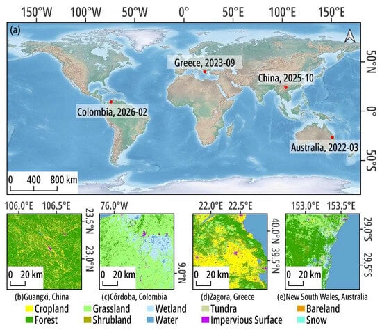
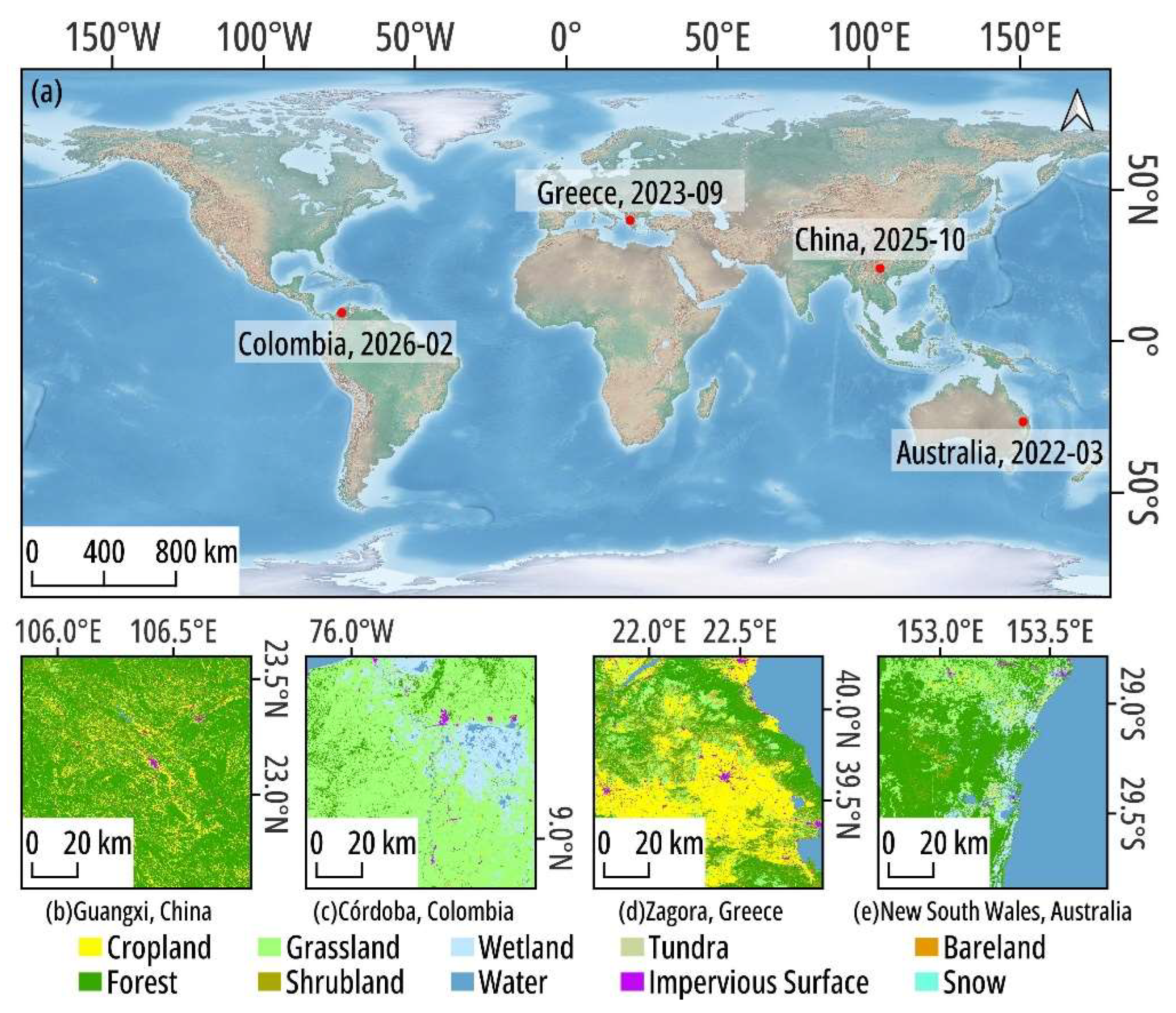
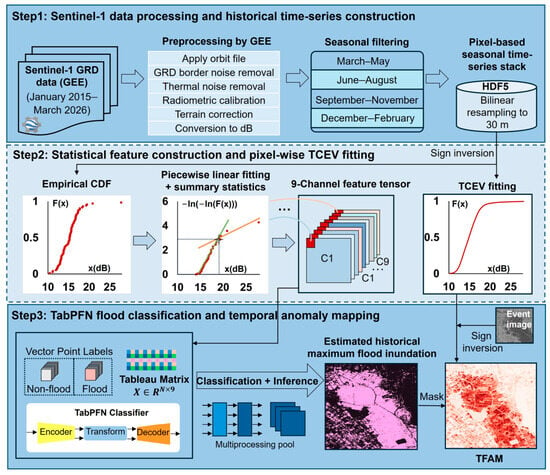
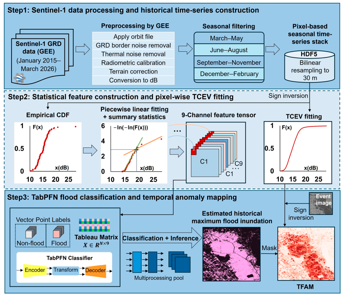
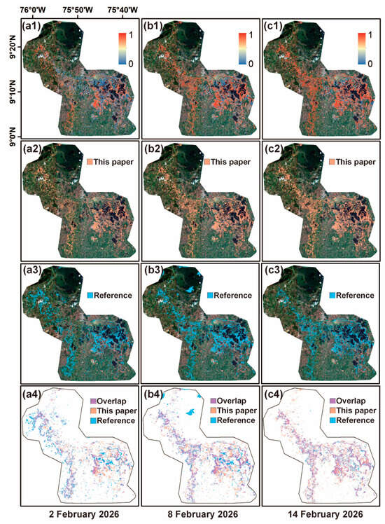
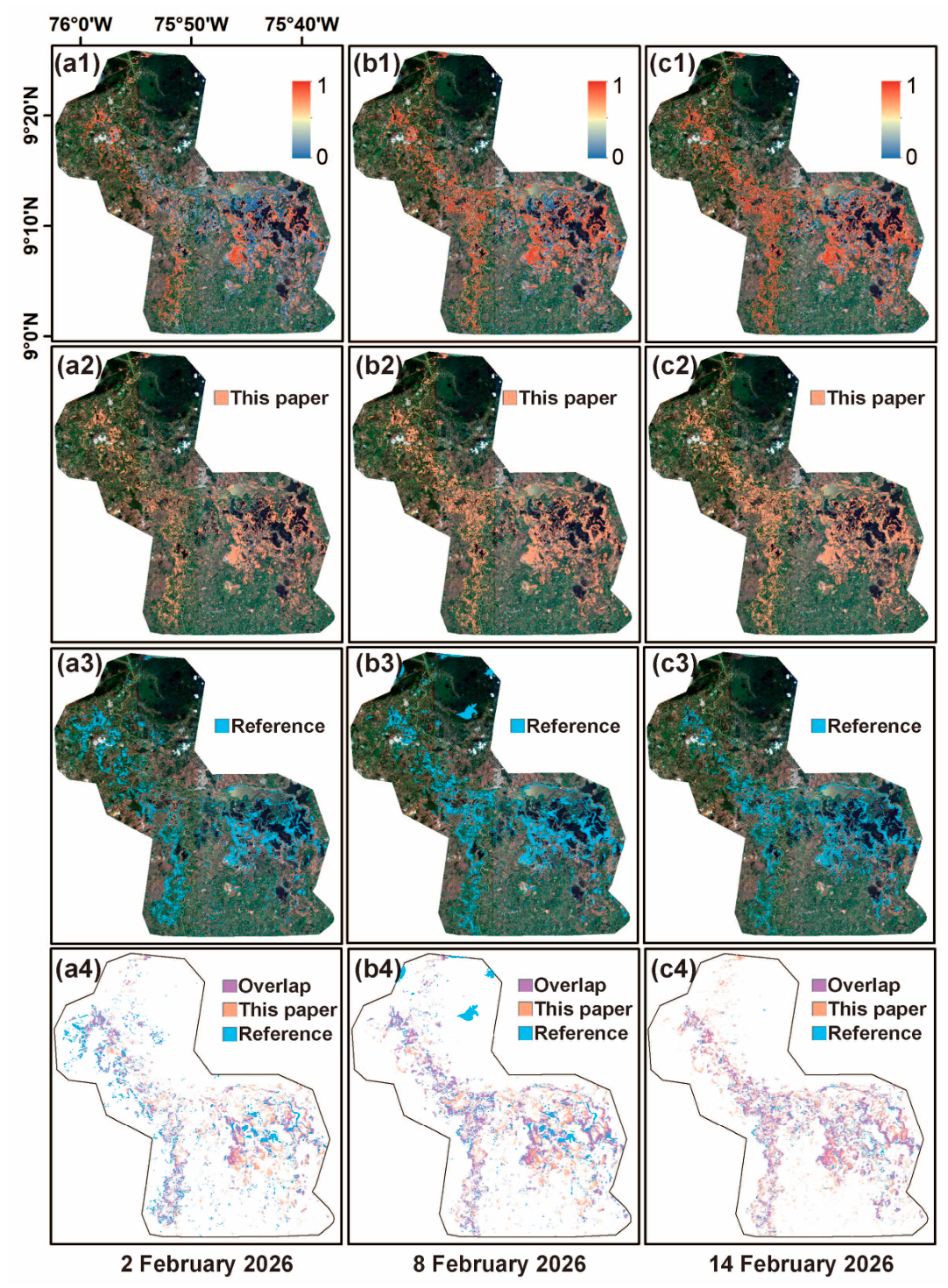
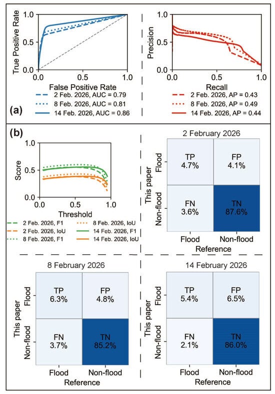
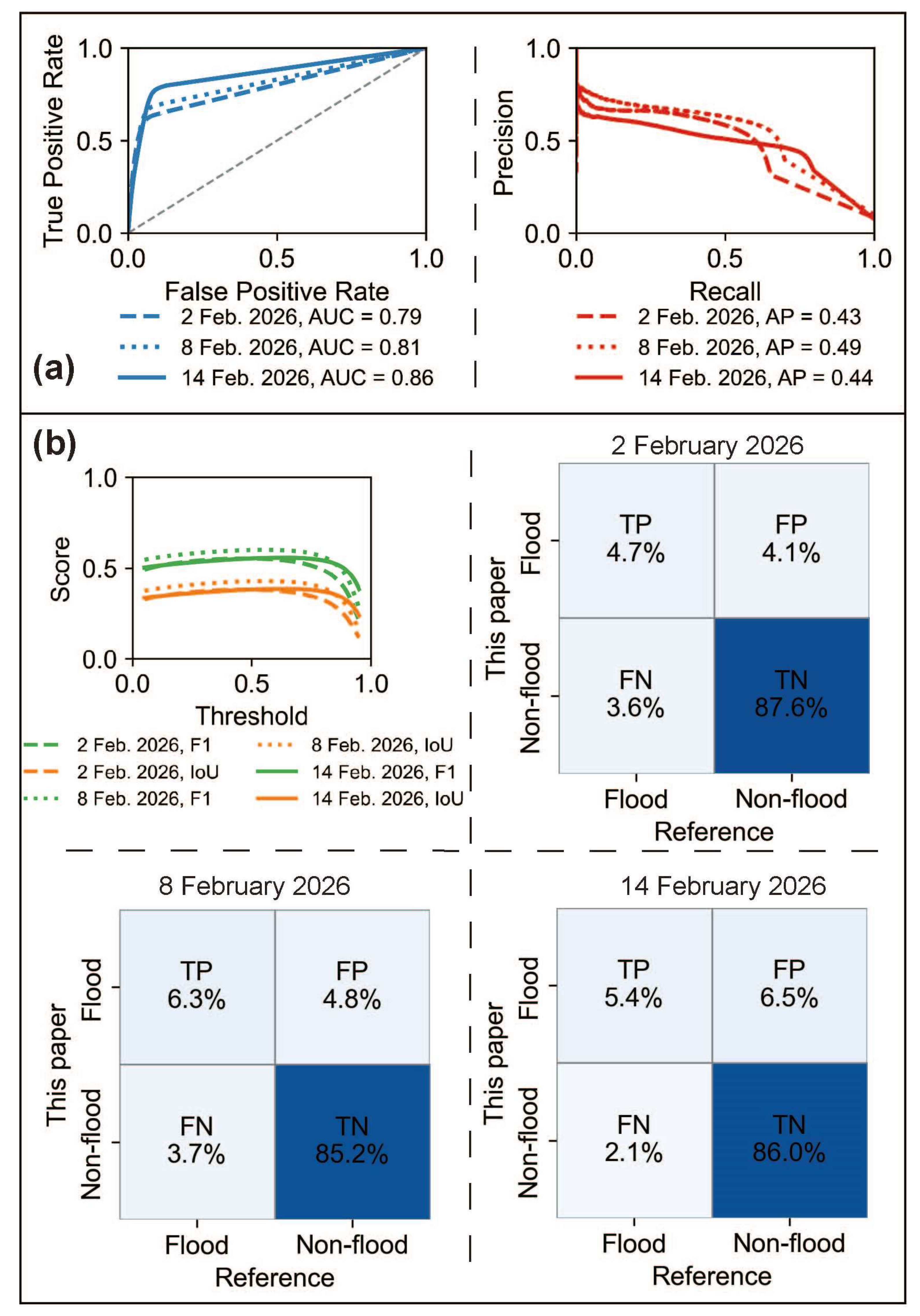
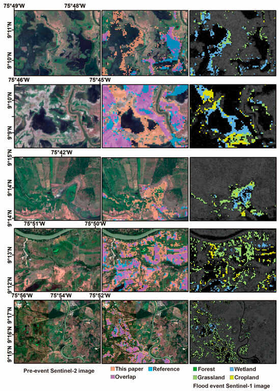
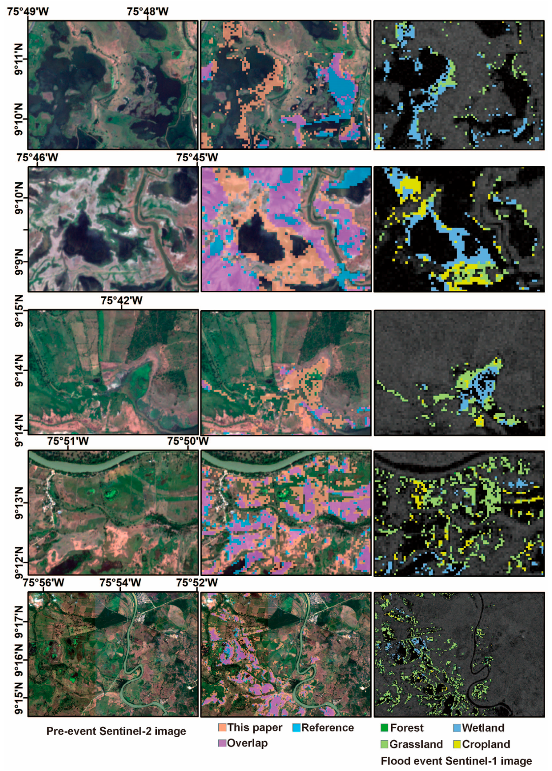
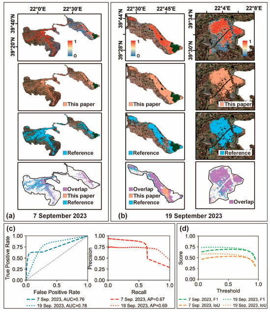
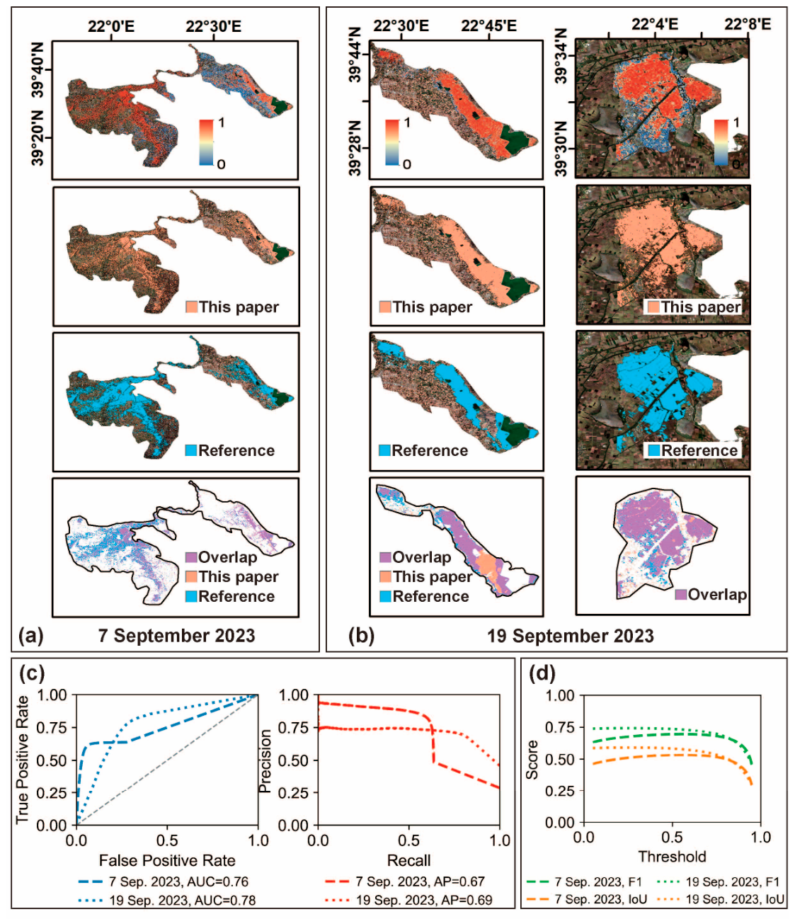
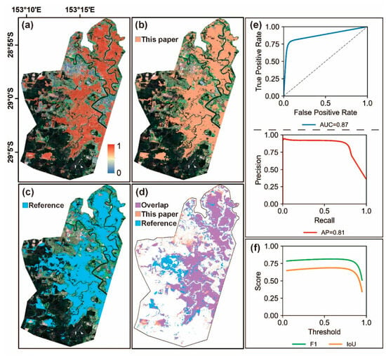
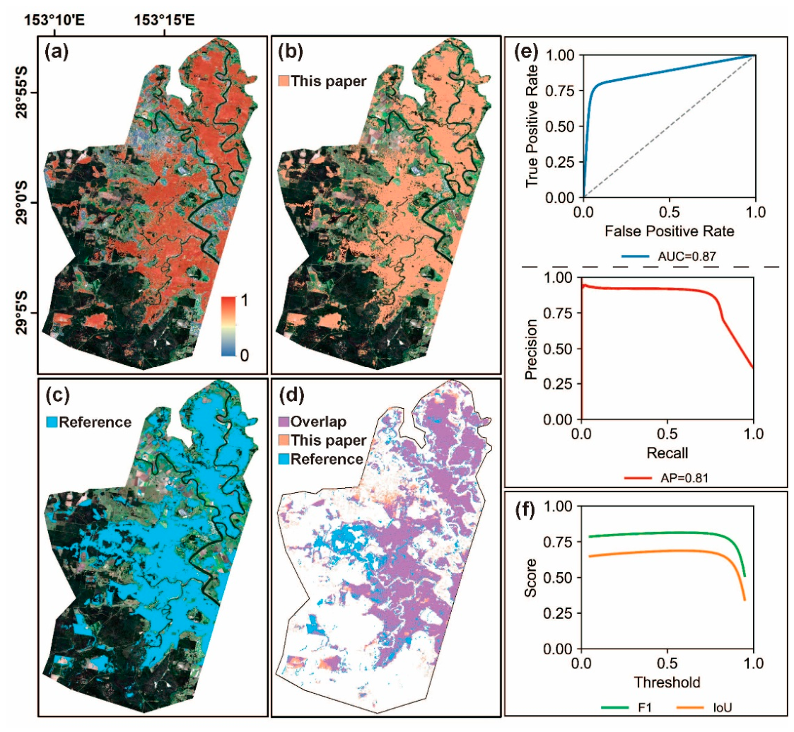
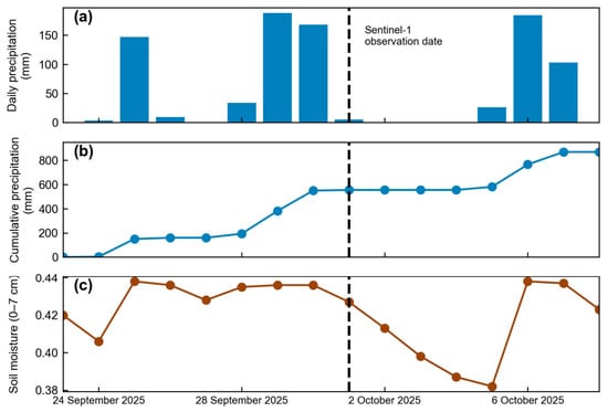
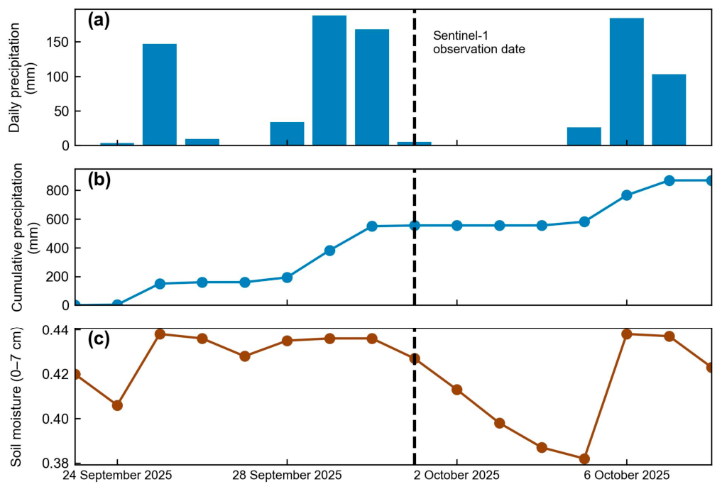
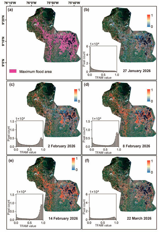
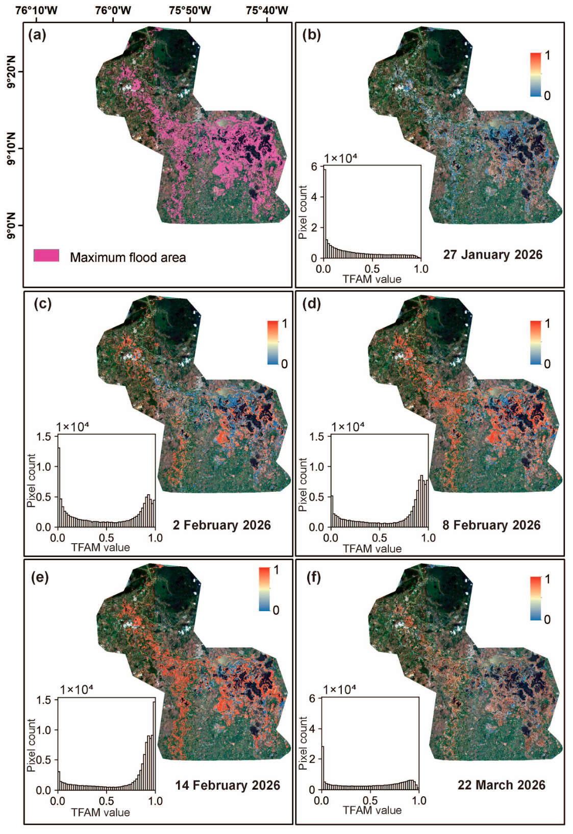
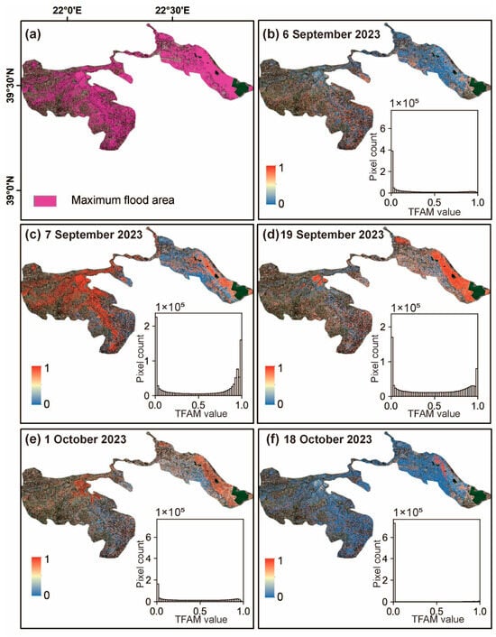
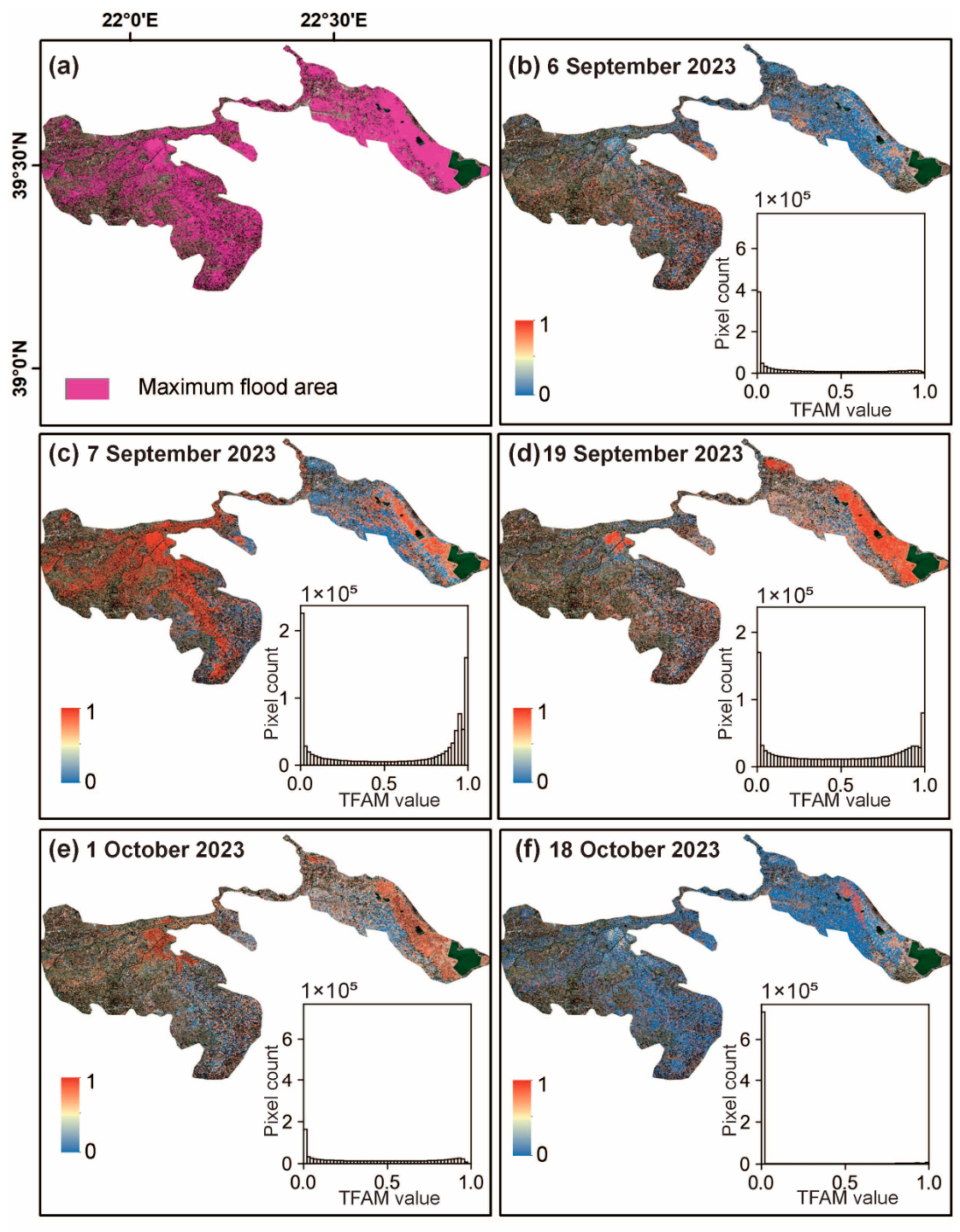
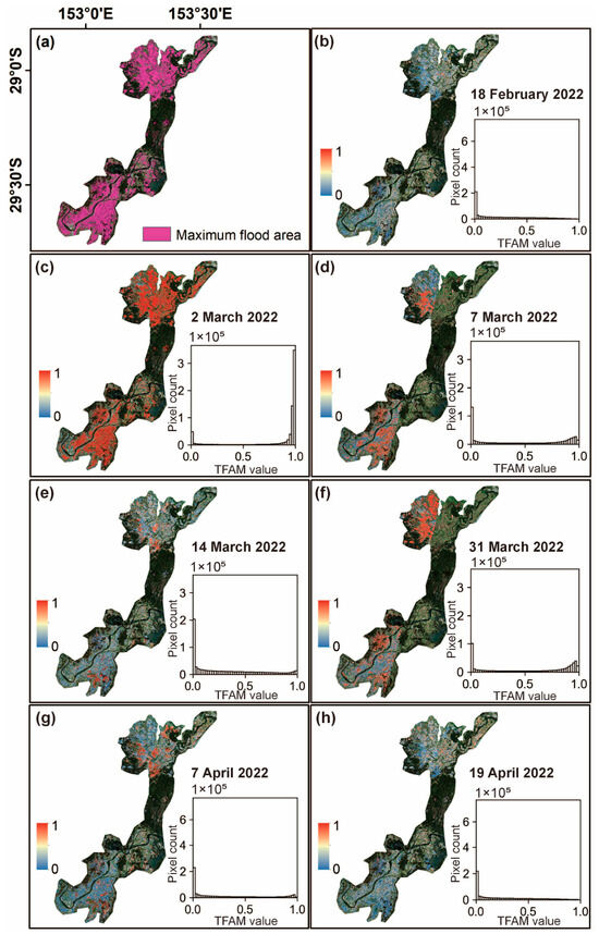
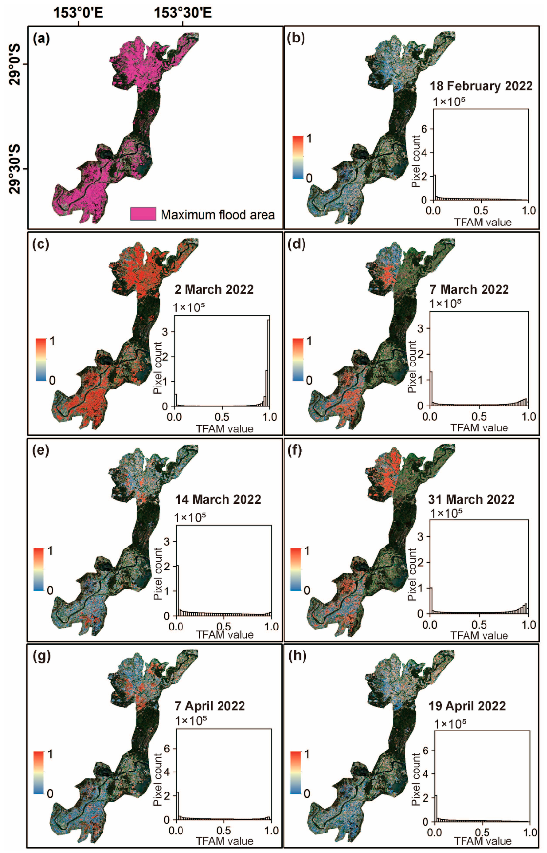
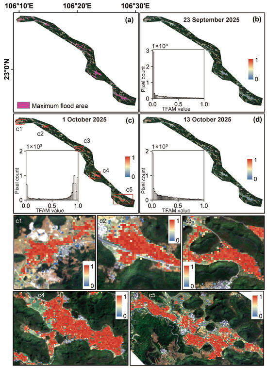
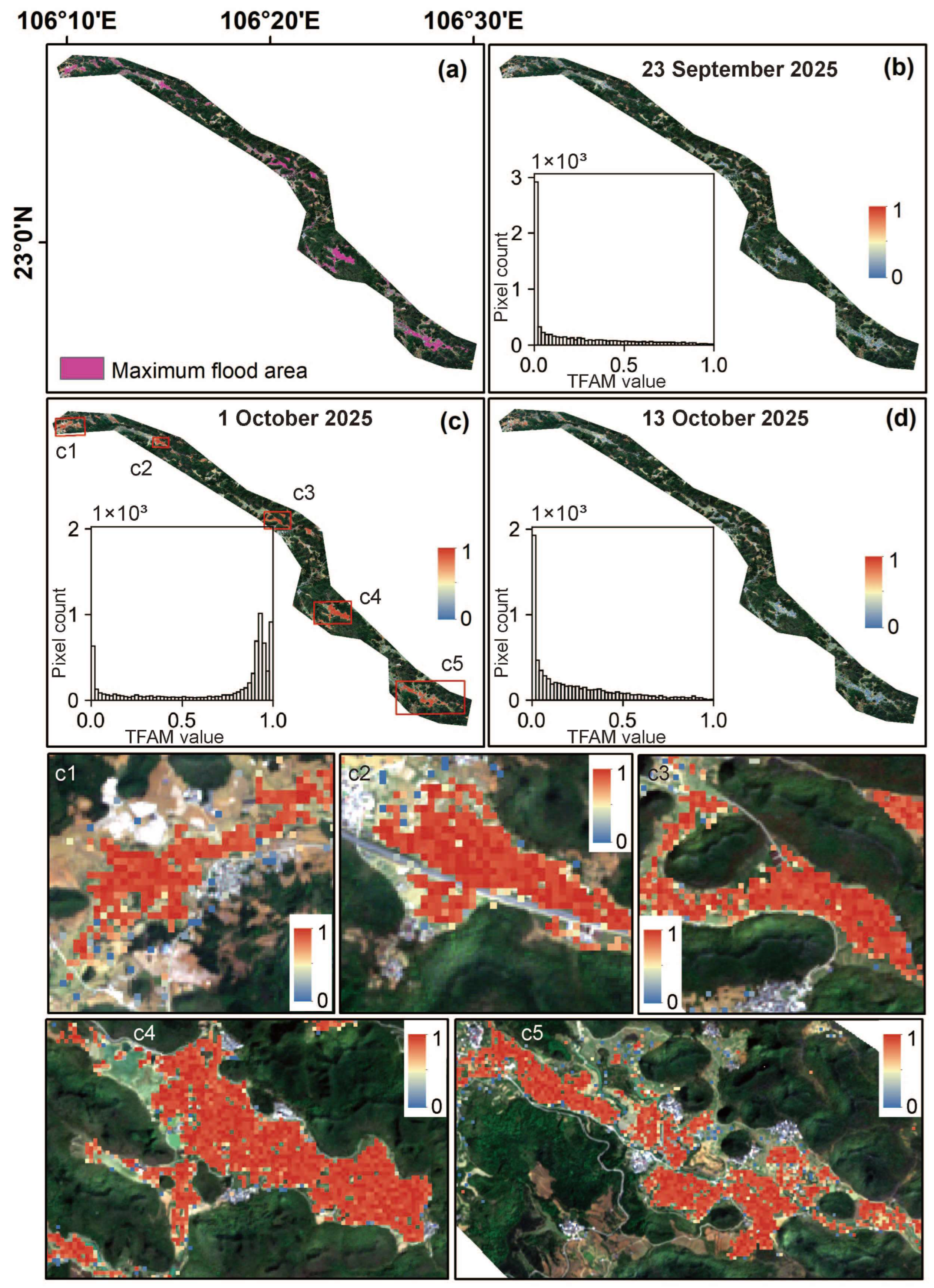

Disclaimer/Publisher’s Note: The statements, opinions and data contained in all publications are solely those of the individual author(s) and contributor(s) and not of MDPI and/or the editor(s). MDPI and/or the editor(s) disclaim responsibility for any injury to people or property resulting from any ideas, methods, instructions or products referred to in the content. |
© 2026 by the authors. Licensee MDPI, Basel, Switzerland. This article is an open access article distributed under the terms and conditions of the Creative Commons Attribution (CC BY) license.