Physics-Informed Liquid Neural Network Emulator for CRTM with Atmospheric-Layer Jacobian Capability

Highlights

What are the main findings?

• The proposed CRTM-LNN emulator learns layer optical-depth increments (Δτ) through adaptive, ODE-inspired liquid dynamics rather than directly mapping atmospheric states to radiances. Coupling these predictions with an analytic, differentiable radiative-transfer solver preserves the complete physical pathway from layer optical depth to cumulative optical depth, transmittance, weighting functions, brightness temperatures, and Jacobians.
• The CRTM–LNN emulator achieves global, channel-mean BT biases (CRTM_LNN − CRTM) below 0.1 K in magnitude, although regional bias magnitudes reach several tenths of a kelvin for selected channels and latitude bands. It also achieves correlation coefficients above 0.97 for key radiative-transfer quantities at cumulative optical depths below five and up to an 18-fold speedup in forward calculations. Compared with a conventional MLP emulator, the CRTM-LNN produces smoother, better-localized, and more vertically coherent temperature Jacobians, while two-GPU automatic differentiation is approximately five times faster than CPU-based CRTM tangent-linear calculations.

What are the implications of the main findings?

• The ODE-driven, end-to-end differentiable framework preserves key aspects of CRTM’s physical functionality and interpretability while enabling efficient, batched GPU-based Jacobian calculations through automatic differentiation.
• These capabilities provide a foundation for future applications in satellite radiance simulation, atmospheric retrievals, observation-minus-background monitoring, and variational data assimilation.

Abstract

Physics-based fast radiative transfer models (RTMs), such as the Community Radiative Transfer Model (CRTM), face increasing computational demands from growing satellite data volumes and model complexity. We developed a physics-informed Liquid Neural Network emulator for CRTM (CRTM-LNN) that draws on continuous dynamical-system concepts while retaining physical interpretability. The framework combines an Ordinary Differential Equation (ODE)-inspired Liquid Neural Network for layer-by-layer optical-depth modeling with an analytic, differentiable radiative-transfer solver. This design preserves the explicit optical-depth-to-radiance pathway and incorporates physical constraints directly into the forward calculation. In the implementation evaluated in this study, the LNN uses discrete hidden-state updates on the fixed European Centre for Medium-Range Weather 91-layer (ECMWF91L) grid under clear-sky, absorption-only assumptions. Evaluation using Infrared Atmospheric Sounding Interferometer (IASI) observations and ECMWF91L forecast profiles shows that CRTM–LNN closely reproduces the reference CRTM simulations, with global, channel-mean brightness-temperature biases below 0.1 K in magnitude. Regional bias magnitudes nevertheless reach approximately 0.2–0.4 K for selected channels and latitude bands. Correlations with CRTM exceed 0.97 for cumulative optical depth, transmittance, and weighting functions in regimes with cumulative optical depth below five. It accelerates forward calculations by up to 18-fold and efficiently generates Jacobians through automatic differentiation. Compared with a conventional multilayer perceptron CRTM emulator, CRTM-LNN produces smoother and more physically consistent Jacobians, with improved vertical localization and fewer spurious oscillations. Absolute centroid-pressure errors for temperature Jacobians are reduced across all evaluated channels, ranging from 1.77 to 5.01 hPa for CRTM-LNN versus 5.88–8.17 hPa for CRTM–MLP, although the magnitude of improvement varies by channel. These results highlight the potential of the integrated CRTM–LNN framework, which combines ODE-driven neural emulation with physics-based radiative-transfer modeling, to provide a scalable foundation for atmospheric retrievals, satellite data assimilation, and near-real-time radiative-transfer applications. Current limitations and opportunities for extension to more complex radiative processes are also discussed.

1. Introduction

Atmospheric radiative transfer models, such as the Community Radiative Transfer Model (CRTM), are among the most widely used operational models in satellite remote sensing and serve as the radiative-transfer engine for numerous satellite data assimilation, retrievals, radiance monitoring, and instrument calibration/validation (Cal/Val) [1,2,3]. Accurate simulation of satellite radiances is essential for fully exploiting these observations, as it establishes the physical link between atmospheric-state variables and measured radiances. For retrieval and data-assimilation applications, accurate atmospheric-state Jacobians are also essential because they quantify the sensitivity of simulated radiances to changes in temperature, water vapor, trace gases, and surface properties.

As both the volume and spectral resolution of satellite observations continue to increase, CRTM computations have become a major bottleneck for large-scale processing, near-real-time applications, and next-generation hyperspectral observing systems, for example, the Infrared Atmospheric Sounding Interferometer (IASI), its new generation IASI-NG, and the Geostationary Infrared Sounder, as well as the emerging hyperspectral microwave sounders. These instruments provide thousands to tens of thousands of spectral measurements that contain rich information about atmospheric temperature, humidity, and trace gases, playing a central role in NWP, atmospheric composition monitoring, climate research, and environmental applications [4,5,6,7]. Their rapidly increasing data volume creates substantial computational demands not only for forward radiance simulation but also for the repeated Jacobian calculations required by iterative retrieval and assimilation systems.

The rapid development of artificial intelligence and machine learning (AI/ML) technologies has driven growing interest in neural-network-based CRTM emulators, which have demonstrated substantial computational acceleration while maintaining high forward-prediction accuracy across diverse remote-sensing applications [8,9,10,11,12,13,14,15,16,17,18].

However, many existing AI-based radiative-transfer emulators use direct-output formulations that map atmospheric and surface variables directly to top-of-atmosphere radiances or brightness temperatures (BTs). For example, Liang et al. (2022) [13] developed FCDN-CRTM, a fully connected neural network emulator for the 22 Advanced Technology Microwave Sounder (ATMS) channels, with atmospheric and surface Jacobians obtained by differentiating the learned atmospheric-state-to-BT mapping. Liu and Liang (2023) [14] extended this formulation by introducing a Jacobian-matching loss that constrains the neural-network-derived sensitivities against CRTM reference Jacobians during training. Although these approaches achieve strong forward accuracy and can provide useful radiative sensitivities, intermediate quantities governing radiance formation—such as layer and cumulative optical depth, atmospheric transmittance, and weighting functions—remain implicit in the forward calculation. Consequently, it is difficult to determine whether accurate BT predictions and Jacobians are supported by physically accurate vertical absorption structures. This limitation has motivated complementary approaches that represent the ordered vertical structure of atmospheric radiative transfer more explicitly. One such direction is the use of sequence-based architectures that propagate information through successive atmospheric layers.

Ukkonen (2022) [15] developed a bidirectional recurrent architecture, implemented using Gated Recurrent Unit (GRU) layers, that propagates information vertically through the atmospheric column and predicts radiative fluxes at atmospheric-layer interfaces. Like other conventional discrete recurrent architectures, including Long Short-Term Memory (LSTM) networks, this GRU-based model employs predefined state-transition and gating equations, although its hidden states and gate values remain input-dependent. Moreover, recurrence alone does not explicitly preserve the intermediate optical quantities or the physical pathway of radiative transfer, motivating complementary hybrid approaches that couple learned optical properties with a physical radiative-transfer solver.

Following this hybrid strategy, Veerman et al. (2021) [17] trained feed-forward neural networks to predict layer-local optical quantities, including optical depth, single-scattering albedo, and Planck-source terms, which were subsequently supplied to the Radiative Transfer for Energetics and Rapid Radiative Transfer Model for General Circulation Model Applications–Parallel (RTE+RRTMGP) solver for shortwave and longwave flux calculations. This approach preserves a physical solver after the learned gas-optics component, but each layer is treated independently by the neural model, without a recurrent hidden state that propagates vertical context through the atmospheric column. Kawahara et al. (2022) [18] demonstrated that opacity and spectral radiative-transfer calculations can be implemented within an end-to-end automatically differentiable framework, allowing sensitivities to atmospheric temperature–pressure profiles and molecular abundances to propagate through the physical calculation. Although ExoJAX—the developed Graphics Processing Unit (GPU)/Tensor Processing Unit (TPU) compatible package for automatic differentiation and accelerated linear algebra—is not a CRTM neural emulator, it provides an important precedent for retaining an explicit differentiable radiative-transfer solver when atmospheric sensitivities are required.

These previous studies establish important foundations for direct-output emulation, recurrent vertical modeling, optical-property prediction, Jacobian supervision, and differentiable radiative transfer. Taken together, they also identify two important capabilities for next-generation radiative-transfer emulators: an effective representation of information propagation through the ordered atmospheric column and an explicit differentiable pathway that connects atmospheric optical properties to radiances and sensitivities. These requirements motivate the exploration of neural architectures whose internal state evolution is naturally suited to layer-by-layer dynamical processes.

Liquid Neural Networks (LNNs) have recently emerged as a promising framework for modeling complex dynamical systems through Ordinary Differential Equations (ODE)-inspired hidden-state evolution [19]. Closely related to Neural ODEs [20], LNNs parameterize a nonlinear state tendency that depends on the current input and hidden state and numerically advance the resulting dynamics through an ordered sequence. Thus, although their trainable parameters remain fixed after training, the hidden-state trajectory and effective update vary with each input. Conventional RNN, GRU, and LSTM architectures also generate input-dependent hidden states and gates, but they do so through predefined discrete state-transition equations rather than an explicitly ODE-inspired dynamical-system formulation, and do not, when used as direct-output emulators, necessarily preserve the complete optical-depth-to-radiance pathway. Furthermore, the LNN provides a natural connection to atmospheric radiative transfer, in which absorption, transmission, and emission evolve cumulatively through successive atmospheric layers. Although the LNN hidden state is a latent representation rather than a physical radiative quantity itself, its dynamical formulation provides a structured mechanism for representing layer-to-layer dependencies and analyzing how information propagates through the atmospheric column. Motivated by the correspondence between dynamical-system modeling and the vertically cumulative nature of radiative transfer, we extend the LNN concept from temporal evolution to the atmospheric vertical coordinate through a layer-by-layer optical-depth Liquid Neural Network (LNN-LOD). The atmospheric layers are treated as an ordered sequence extending from the top of the atmosphere to the surface, along which a latent radiative state is propagated. At each layer, a bounded, input-dependent gate modulates the ODE-inspired hidden-state update according to the local thermodynamic and compositional conditions and the vertical context carried from preceding layers. The resulting latent states are mapped to channel-dependent layer optical-depth increments, Δτ. The LNN-LOD network’s “liquid” behavior arises from an input- and state-dependent, signed element-wise gate that modulates the learned hidden-state tendency, allowing the latent representations to respond to atmospheric conditions and vertically propagated context. This gate controls the internal latent-state evolution rather than representing physical layer thickness or a direct measure of extinction.

The LNN-LOD is subsequently coupled with an analytic, differentiable radiative-transfer solver to form the proposed CRTM-LNN emulator. Rather than directly mapping atmospheric states $\left(\mathit{X},\mathit{g}\right)$ to top-of-atmosphere (TOA) brightness temperatures (BTs), the framework preserves the explicit radiative-transfer pathway: Δτ → cumulative optical depth → transmittance → weighting function → radiance/BT. The learned and analytic components therefore have complementary roles: LNN-LOD models the atmospheric-state-to-optical-depth relationship, whereas the analytic solver determines how the predicted optical depths produce cumulative absorption, transmittance, atmospheric weighting functions, atmospheric and surface radiance contributions, and TOA BTs. During training, the predicted layer optical depths and solver-generated BTs are jointly constrained. The Δτ-based losses preserve the local magnitude and cumulative vertical structure of atmospheric absorption, while the BT loss propagates backward through the differentiable solver to improve the radiometric consistency of the optical-depth predictions.

We summarize the existing AI-based radiative-transfer emulators discussed above and compare their principal characteristics with those of the CRTM-LNN framework developed in this study in

Table 1. A compact related-work comparison table.

Emulator Category	Typical Learned Output	Treatment of Atmospheric Vertical Structure	Physical Pathway	Jacobian Source	Ref.
Direct MLP emulator	Radiance or BT	Flattened/static mapping	Usually not retained	Derivative of learned BT mapping	e.g., [12,13]
Loss-based physics-informed MLP emulator	Often radiance or BT	Architecture dependent	Physics mainly imposed through losses, such as Jacobian loss	Architecture dependent	e.g., [14]
RNN emulator (LSTM or GRU)	Radiance, BT, or sequential output	Fixed-form recurrent cell based on predefined discrete state-transition structures	Depends on formulation	Derivative of learned mapping	e.g., [15]
Hybrid Differentiable-physics emulator	Optical or state variables	Architecture dependent	Explicit differentiable physical solver	Differentiation through the complete learned- solver pathway	e.g., [17,18]
CRTM-LNN	Layer Δτ, BT	ODE-inspired, input-dependent liquid evolution	$\left(\mathit{X},\mathit{g}\right)\to ∆{\tau }_{\upsilon ,k}\to {\tau }_{\upsilon ,k}\to {\mathcal{T}}_{\upsilon ,k}\to I_{\upsilon ,TOA}\to BT$	Autograd through learned Δτ and an analytic RT solver	e.g., [19]

.

The primary objective of this study is not to conduct a general comparison or establish a universal ranking among LNN, MLP, and RNN architectures. Rather, our goal is to develop and evaluate a new CRTM-LNN emulator that combines ODE-inspired layer-optical-depth modeling with an explicit differentiable radiative-transfer pathway and thereby provides the potential to generate physically structured atmospheric Jacobians through automatic differentiation. These Jacobians account for both the learned dependence of optical depth on the atmospheric state and the analytically prescribed dependence of radiance on optical depth. The conventional direct-BT MLP is included only as a supporting reference for illustrating the value of retaining intermediate optical quantities and an explicit radiative-transfer pathway; it is not intended as an exhaustive architectural comparison. The principal contribution of CRTM-LNN is therefore the integration of ODE-inspired vertical optical-depth dynamics, joint Δτ–BT supervision, and analytic radiative-transfer coupling within an end-to-end differentiable CRTM emulator.

To evaluate CRTM-LNN, we focused on 111 channels within the IASI 15 μm CO₂ absorption band (645–672.5 cm⁻¹). This spectral range is critical for hyperspectral infrared temperature sounding, serving as a rigorous benchmark for radiative-transfer emulators. Since radiances from these channels are primarily driven by CO₂ absorption, with minimal influence from surface emissivity and cloud contamination, differences between emulator predictions and CRTM simulations directly reflect the model’s capacity to represent vertical radiative processes and layer-to-layer interactions. Furthermore, the strong absorption and inherent nonlinearity of this spectral region make it an ideal testbed for evaluating how well the proposed framework preserves physically realistic optical-depth structures, radiative sensitivities, and overall hyperspectral consistency, free from the added complexity of scattering.

In this paper, the detailed data and methodology, including the detailed gate formulation, stabilized two-stage update, and network architecture of LNN-LOD, are presented in Section 2. Section 3 provides an assessment of the model’s performance, while Section 4 discusses the results and their implications. Finally, conclusions are summarized in Section 5. To maintain conciseness, we use “CRTM-LNN” or “CRTMLNN” interchangeably to denote the physics-informed, radiative transfer consistent AI emulator, for which LNN-LOD serves as the core framework.

2. Methodology, CRTM-LNN Implementation, and Dataset

2.1. CRTM-LNN Implementation with Layer Optical Depth Modeling (LNN-LOD)

CRTM-LNN is especially suited for hyperspectral satellite sounder observations, and it adopts a physics-informed modeling strategy for radiative-transfer emulation. At the core of the framework is the LNN-LOD, which learns the layer-by-layer evolution of latent radiative-transfer states through adaptive liquid dynamics. By propagating these hidden states along the atmospheric column, the LNN-LOD naturally represents the cumulative absorption and emission processes governing atmospheric radiative transfer and provides a physical representation of the vertical atmospheric structure. The latent radiative-transfer states are subsequently mapped to layer optical-depth increments (Δτ), which serve as one primary physical quantity predicted by the network. To ensure physical interpretability, the predicted Δτ is coupled with an analytic radiative-transfer solver that reconstructs cumulative optical depth, transmittance, weighting functions, and top-of-atmosphere radiances/BTs. The LNN-LOD captures the cumulative nature of atmospheric radiative transfer through its sequential hidden-state evolution, allowing information from preceding layers to propagate throughout the atmospheric column.

The radiative transfer of the atmosphere is briefly discussed here. Given the vertical state $x_k$ by

$$x_k={[T_k,q_k,O_{3,k},{CO}_{2,k},p_k]}^T,k=1,\dots ,L$$

(1)

The atmospheric state vector X:

$${X=\left\{x_k\right\}}_{k=1}^L$$

(2)

where k is the vertical layer index, with k = 1 at the TOA; k = L at the ground surface. $T_k$ is temperature, $q_k$ stands for water vapor specific humidity, O_3,k is ozone mixing ratio, CO_2,k is carbon dioxide mixing ratio, $p_k$ is the layer pressure.

The auxiliary viewing-geometry and surface-boundary vector:

$$g=[sec\_sza,sec\_sa,saa,psfc,skt].$$

(3)

where sec_sza is the secant of the sensor zenith angle, sec_sa is the secant of the sensor scan angle, saa is the sensor azimuth angle, psfc is the surface pressure, and skt is the surface skin temperature. Surface pressure is physically relevant because it defines the lower boundary and effective extent of the atmospheric column. Surface skin temperature primarily controls the surface radiative boundary and has only limited direct influence on most channels in the strongly absorbing 15 μm CO₂ band; nevertheless, it was retained as a general surface-context variable that may provide information for less opaque band-edge channels or lower-atmospheric regimes correlated with surface conditions. Sensor zenith angle determines the physical slant path in the analytic solver, whereas scan angle describes the instrument sampling position and may contain partially redundant geometric information. Sensor azimuth has no direct scalar radiative effect under the present assumptions and was included only as general observation context. Please see Section 4 for discussion.

Together, (X, g) fully define the inputs to the radiative-transfer system. The targets (Y) of the training dataset used in this study are derived from CRTM ([21]; version 3.0, [22]) simulations for both BT and layer optical depth.

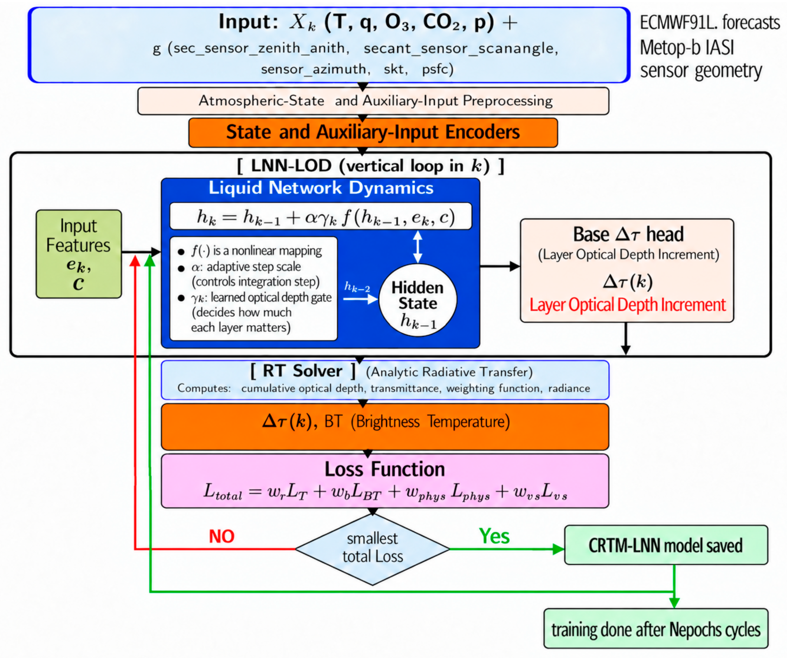
An overview of the LNN-LOD architecture is shown in Figure 1, and the detailed components are described in the following subsections.

2.1.1. The CRTM and LNN Connection

The radiative transfer in the atmosphere is the first-order differential equation when only considering the atmospheric absorption and emission:

$$\mu {\displaystyle \frac{d{I}_{\upsilon }(\tau ,\mu )}{d\tau }}=I_{\upsilon }(\tau ,\mu )-B_{\upsilon }(T)$$

(4)

And the monochromatic optical depth ${\tau }_{\upsilon }$ satisfies the differential relation:

$${\displaystyle \frac{d{\tau }_{\upsilon }}{dz}}={-k}_{\upsilon }(z)\rho (z)$$

(5)

where $I_{\upsilon }$: the intensity of radiation; μ = cosθ, θ: viewing zenith angle; B_υ: the Planck radiance; τ: optical depth; k_υ(z) is the absorption coefficient; $\rho \left(z\right)$ is the absorber density; υ is the wavenumber; and z denotes altitude increasing upward. Therefore, cumulative optical depth is obtained through vertical integration of local-layer contributions.

$${\tau }_{\upsilon }\left(z\right)={\int }_z^{TOA}{k}_{\upsilon }\left(z^{\prime }\right)\rho \left(z^{\prime }\right)d{z}^{\prime }$$

(6)

where TOA denotes the top of the atmosphere. After discretization, this becomes a sequential accumulation process:

$${\tau }_k\left(\upsilon \right)={\sum }_{i=1}^k∆{\tau }_i\left(\upsilon \right),{\tau }_0(\upsilon )=0$$

(7)

where $∆{\tau }_i$ is the vertical optical depth of layer i; the vertical index i,k increases downward from the TOA. ${\tau }_k$ is the cumulative vertical optical depth, with no viewing-angle factor included in this summation. Thus τ’s vertical evolution naturally follows a recursive layer-by-layer integration structure. This is the key motivation for using the LNN-LOD framework. By predicting local-layer optical depth, the model learns to represent effective absorption within individual atmospheric layers. Each prediction depends on both the local encoded atmospheric state and the vertically propagated context carried by the hidden state, rather than exclusively on local-layer properties. Viewing geometry is incorporated through a slant-path factor μ:

$$∆{\tau }_k^{\left(slant\right)}(\upsilon )={\displaystyle \frac{∆{\tau }_k\left(\upsilon \right)}{\mu }}$$

(8)

The atmospheric transmittance can then be reconstructed through cumulative optical depth (Equation (7)):

$${Tr}_k=e^{-{\displaystyle \frac{{\tau }_{phys,k}}{\mu }}}=e^{-{\displaystyle \frac{1}{\mu }}{\sum }_{i=1}^k∆{\tau }_i}=e^{-{\displaystyle \frac{1}{\mu }}{\sum }_{i=1}^k∆{\tau }_i^{\left(slant\right)}}$$

(9)

This formulation is highly compatible with the ODE-like hidden-state evolution in LNN, where information propagates sequentially along the atmospheric column. The framework therefore mimics the physical accumulation process inherent in radiative transfer: local absorption is first computed layer-by-layer, and the total radiative effect emerges through cumulative vertical integration, providing sound physical interpretability of layer-dependent radiative-transfer behavior.

2.1.2. Atmospheric-State and Auxiliary-Input Preprocessing

Before entering the neural-network encoders, the atmospheric-state and auxiliary variables are transformed to improve numerical conditioning and ensure comparable feature scales. For each atmospheric layer, temperature and CO₂ are standardized using their training-data means and standard deviations, whereas water vapor and ozone are first logarithmically transformed to compress their large dynamic ranges and then standardized. Layer pressure is represented by the dimensionless pressure coordinate ${\sigma }_k={\displaystyle \frac{p_k}{psfc}}$. The resulting atmospheric-state vector is

$${\tilde{x}}_k=[{\displaystyle \frac{T_k-{\mu }_T}{{\sigma }_T}},{\displaystyle \frac{{\mathrm{l}\mathrm{o}\mathrm{g}(q}_k+{ϵ}_q)-{\mu }_{logq}}{{\sigma }_{logq}}},{\displaystyle \frac{{\mathrm{l}\mathrm{o}\mathrm{g}(O}_{3,k}+{ϵ}_{O_3})-{\mu }_{log{O}_3}}{{\sigma }_{log{O}_3}}},{\displaystyle \frac{{CO}_{2,k}-{\mu }_{{CO}_2}}{{\sigma }_{{CO}_2}}},{\displaystyle \frac{p_k}{psfc}}]$$

where ϵ is a small constant to ensure numerical stability: ${ϵ}_q={10}^{-10}$ and ${ϵ}_{O_3}={10}^{-12}$. The five raw viewing-geometry and surface-boundary variables are separately transformed into a six-dimensional auxiliary feature vector. The sensor-zenith and scan-angle secants are shifted by one so that the nadir condition corresponds to zero. Sensor azimuth is represented by its sine and cosine components to preserve angular continuity, while surface pressure and skin temperature are scaled to dimensionless values of approximately order one. The resulting vector is

$$\tilde{g}=[sec\_sza-1,sec\_sa-1,\sin \left(saa\right),\mathrm{c}\mathrm{o}\mathrm{s}(saa),{\displaystyle \frac{psfc}{1000}},{\displaystyle \frac{skt-250}{50}}].$$

These transformations reduce scale disparities, account for the periodicity of azimuth, and provide dimensionless, numerically stable inputs to the atmospheric-state and auxiliary-input encoders.

2.1.3. State and Auxiliary-Input Encoder

Within the proposed CRTM-LNN framework, the atmospheric-state and auxiliary-input encoders form a dual-branch input-processing module for the LNN-LOD. At each atmospheric layer, the state encoder projects five preprocessed variables ${\tilde{x}}_k$—temperature, water vapor, ozone, CO₂, and normalized pressure ${\sigma }_k$—into a 64-dimensional latent representation ${\mathit{e}}_k$ that describes the local thermodynamic and compositional state. In parallel, the auxiliary-input encoder processes six preprocessed viewing-geometry and surface-boundary features $\tilde{g}$ through two fully connected layers to produce a 64-dimensional context vector $\mathit{c}$.

The two encoded representations provide complementary information to the LNN-LOD. The atmospheric-state representation characterizes the local conditions at each layer, whereas the auxiliary representation supplies profile-level viewing-geometry and surface-boundary context. Both are incorporated into the hidden-state tendency and adaptive-gate calculations, allowing the layer-by-layer state evolution to respond jointly to local atmospheric properties, vertically propagated information, and observation-specific conditions.

2.1.4. LNN-LOD for Vertical Optical-Depth Dynamics

Although the proposed LNN-LOD is inspired by Liquid Time-Constant (LTC) networks [19], its hidden-state evolution differs substantially from the classical LTC formulation. The original LTC dynamics are typically expressed as

$${\displaystyle \frac{dh}{dt}}=-\left[{\displaystyle \frac{1}{{\tau }_c}}+f\left(h,\mathit{e},\mathit{c}\right)\right]h\left(t\right)+f\left(h,\mathit{e},\mathit{c}\right)A$$

where ${\tau }_c$ is the time constant, A is the equilibrium state, $f\left(·\right)$ is a learned nonlinear mapping that dynamically modulates the system behavior. $\mathit{e},\mathit{c}$ denote the compatible 64-dimensional latent representations obtained by projecting the preprocessed atmospheric state $\tilde{x}$ and auxiliary inputs $\tilde{g}$ through their respective encoders. The first term represents leakage or relaxation toward equilibrium, while the second term represents the input-driven forcing. The hidden state evolves through a balance between a state-dependent decay term and a nonlinear forcing term.

For radiative-transfer applications involving cumulative optical depth, the governing equation is an accumulation process as shown in Equation (6), i.e.,

$${\tau }_{k+1}\left(\upsilon \right)={\tau }_k\left(\upsilon \right)+k_v\left(k\right)\rho \left(k\right){∆z}_k$$

where $k_v$ is the absorption coefficient, $\rho$ is the absorber density, and ${∆z}_k$ is the layer thickness. Since optical depth only accumulates and does not physically decay or leak, the leakage term in the LTC formulation can be removed. In this study, the removal of the explicit leakage term is an architectural design choice inspired by optical-depth accumulation, rather than a consequence of the radiative-transfer equation. The resulting LTC-inspired optical depth model becomes:

$${\displaystyle \frac{dh}{dt}}=f\left(h,\mathit{e},\mathit{c}\right)A$$

As a result, we model the vertical evolution of absorption using a Liquid Neural Network for layer optical depth modeling. As an initial investigation of the LNN-LOD framework for radiative-transfer modeling, this study focuses on absorption-dominant atmospheric conditions, allowing the proposed architecture and its radiative-transfer consistency to be evaluated without the additional complexity introduced by scattering processes.

Let $h_k$∈$R^H$ be the hidden state at layer k. The hidden states are latent radiative-transfer representations that encode the evolving atmospheric and geometric context across layers. Therefore, the dynamics are defined by an ODE-like update that is inspired by the optical-depth propagation equation, different from the classical LTC:

$$h_k=h_{k-1}+\alpha {\gamma }_{k}f(h_{k-1},{\mathit{e}}_k,\mathit{c})$$

(10)

Here $\alpha$ denotes the effective step scale, obtained by multiplying a learnable step-scale parameter ${\mathsf{\alpha }}_0$ by the bounded auxiliary conditioning factor:

$$\begin{gathered} \alpha ={\mathsf{\alpha }}_0{g}_{scale} \\ {g}_{scale}={\displaystyle \frac{sec\_sza}{1.0+1.5sec\_sza+{10}^{-8}}}, \end{gathered}$$

which satisfies $0.4\le g_{scale}\le 2/3$ for sensor zenith angles $0^{\mathrm{o}}\le se{c}_{sza}\le {90}^{\mathrm{o}}$.

In the proposed LNN, hidden-state evolution across atmospheric layers is implemented through discrete, ODE-inspired updates. The nonlinear term $f\left(h_{k-1},{\mathit{e}}_k,\mathit{c}\right)$ represents the learned hidden-state tendency, conditioned on the current hidden state, local atmospheric inputs, and scene-and-geometry information, rather than a direct physical radiative contribution. The adaptive gate ${\gamma }_k$ is a learned, input- and state-dependent vector whose elements satisfy −0.5 < ${\gamma }_k$ < 0.5. The product $\alpha {\gamma }_k$ provides signed, element-wise scaling of the learned hidden-state tendency, modulating the magnitude of each element and potentially reversing its sign. Because the gate depends on the current input and hidden state, this modulation allows different latent features to respond differently to atmospheric conditions and vertically propagated context. Here, “adaptive” refers to input- and state-dependent modulation of the latent dynamics, rather than adaptive selection of numerical integration steps. Neither the gate nor the product $\alpha {\gamma }_k$ is assigned the physical meaning of optical depth or layer thickness. The prescribed updates proceed on the fixed ECMWF91L grid without skipping layers or changing their spacing. Thus, the formulation provides input-conditioned evolution of continuous-valued hidden states through discrete layer-by-layer updates; “continuous-valued” refers to the hidden-state variables, not continuous resolution of the vertical coordinate. Please see Appendix A for more details about ${\gamma }_k$ and $f\left(h_{k-1},{\mathit{e}}_k,\mathit{c}\right)$.

The viewing geometry enters the LNN through two complementary conditioning pathways: a learned scene-and-geometry embedding, $\mathit{c}$, and a prescribed bounded angular multiplier, $g_{scale}$. The embedding $\mathit{c}$ allows the hidden-state tendency and adaptive gate to learn interactions among viewing geometry, atmospheric structure, and vertically propagated context, while $g_{scale}$ provides smooth, bounded angular modulation of the discrete hidden-state updates. Together, these pathways combine flexible, scene-dependent learning with an explicit angular dependence in the latent dynamics. The hidden states are learned representations relevant to atmospheric radiative transfer rather than directly prescribed physical variables. Their coupling with the analytic, differentiable RT solver connects optical-depth prediction to transmittance, weighting functions, brightness temperatures, and radiative sensitivities.

Although the network predicts vertical layer optical depth, its intermediate representations can therefore incorporate viewing geometry to condition how radiative-transfer-relevant information evolves across atmospheric layers. Both pathways condition the latent dynamics rather than explicitly transform the optical path; the physical conversion from vertical to slant-path optical depth is applied only once in the RT solver.

In practice, we use an RK2-inspired stabilized integration scheme:

$$h_k^{(1/2)}=h_{k-1}+{\displaystyle \frac{1}{2}}\alpha {\gamma }_{k}f(h_{k-1},{\mathit{e}}_{\mathit{k}},\mathit{c})$$

(11)

$$h_k=h_{k-1}+\alpha {\gamma }_{k}f(h_k^{(1/2)},{\mathit{e}}_{\mathit{k}},\mathit{c})$$

(12)

This formulation mirrors the cumulative nature of optical depth and ensures stable propagation across layers.

Layer optical depths are subsequently derived from these hidden states through a lightweight fully connected prediction head, denoted as ${\Phi }_{base}$, rather than being represented directly by the hidden states themselves. ${\Phi }_{base}$ consists of two linear networks separated by a SiLU activation function, enabling nonlinear feature refinement while maintaining numerical stability and smooth gradient propagation. The resulting output produces the initial layer optical-depth estimate for all spectral channels at atmospheric layer k, $∆{\tau }_k$:

$$∆{\tau }_k={\Phi }_{base}\left(h_k\right)$$

(13)

$∆{\tau }_k$ predicted by the network are in standardized logarithmic space, depending on the local encoded state and on the vertically propagated context carried by the hidden state. They are first transformed from the standardized $∆{\tau }_k$ back to log space $\widehat{∆{\tau }_k}=s∆{\tau }_k+m$, where s and m are the channel-dependent normalization scale and offset, and then converted to physical optical depth using:

$$∆{\tau }_{phys,k}=\mathrm{m}\mathrm{a}\mathrm{x}\{\exp \left[\mathrm{c}\mathrm{l}\mathrm{i}\mathrm{p}\left(\widehat{∆{\tau }_k},-10,4.5\right)\right],{10}^{-8}\}$$

The constants −10 and 4.5 bound the argument of the exponential and therefore restrict the physical layer increment to roughly 4.5 × 10⁻⁵ to 90, while 10⁻⁸ imposes a strictly positive floor. Therefore, $∆{\tau }_{phys,k}\ge 0$ is enforced by construction rather than an additional penalty term.

2.1.5. Analytic RT Solver Coupling

From Equation (4), under absorption-dominant atmospheric conditions, the TOA upward radiance can be calculated using the following equation:

$$I_{\upsilon }^{\uparrow }\left(\tau ,\mu \right)={[\epsilon }_{\upsilon }{B}_{\upsilon }\left(T_s\right)+\left(1-{\epsilon }_{\upsilon }\right)I_{\upsilon }^{\downarrow }\left({\tau }_s,\mu \right)]e^{-{\displaystyle \frac{{\tau }_s-\tau }{\mu }}}+{\int }_{\tau }^{{\tau }_s}{B}_{\upsilon }\left(\mathrm{T}\right)e^{-{(\tau }^{\prime }-\tau )/\mu }{\displaystyle \frac{d{\tau }^{\prime }}{\mu }}$$

(14)

where ${\epsilon }_{\upsilon }$ is the surface emissivity and $I_{\upsilon }^{\downarrow }$ is the downwelling atmospheric radiance reaching the surface. As the first exploration of the physics-informed LNN-LOD framework, we assumed a unit surface emissivity (=1), along with focusing on an absorbing atmosphere. This approximation is appropriate for the selected IASI 15 um (Ch1–Ch111) temperature-sounding channels, whose radiative sensitivities are concentrated in the upper troposphere and lower stratosphere within the strong 15 μm CO₂ absorption band. As a result, the contribution of surface emission and emissivity effects to the TOA radiances is minimal.

Therefore, the discrete upwelling monochromatic radiance at the top of the atmosphere (TOA) is:

$$I_{\upsilon }^{TOA}=B_{\upsilon }\left(T_s\right)e^{-{\tau }_s/\mu }+{\sum }_{k=1}^N{B}_{\upsilon }\left(T_k\right)(e^{-{\tau }_{k-1}/\mu }-e^{-{\tau }_k/\mu })$$

(15)

where $T_s$: surface skin temperature; and $T_k$: air temperature at layer k. The brightness temperature is $BT\left(\upsilon \right)=B^{-1}\left(I\left(\upsilon \right)\right)$. $B^{-1}$ represents the inverse Planck function. Viewing geometry is incorporated through a slant-path factor μ as shown in Equation (8). The transition from latent neural representations to observable BTs is achieved through a differentiable analytic coupling. Once the predicted optical depths ($∆{\tau }_k$) are mapped back from the latent manifold to physical space, they are integrated into the formal solution of the Radiative-Transfer Equation (RTE) as defined in Equation (15).

This architectural design creates a strict separation of concerns between the statistical learning and the physical simulation: The LNN-LOD is tasked solely with modeling the complex, non-linear absorption physics—a high-dimensional mapping problem that traditional look-up tables or parameterizations struggle to capture efficiently. By predicting $∆{\tau }_k$ directly, the network is forced to learn the intrinsic optical properties of the atmospheric state. The actual propagation of radiation through the layers is handled by an analytic solver. Because this solver is based on the fundamental physics of emission and transmission, the resulting BT is guaranteed to be physically consistent with the predicted optical depths. This eliminates the “black box” risk where a standard neural network might predict a radiance that violates the laws of thermodynamics (e.g., producing upwelling radiance higher than the source function). Since the RT solver in Equation (15) is mathematically analytic, its gradients can be propagated backward during training. This allows the loss signal from the final BT error to directly refine the optical-depth predictions, ensuring that the entire system is optimized for end-of-pipe accuracy while maintaining internal physical integrity.

Please note that the analytic radiative-transfer solver used in CRTM-LNN is based on the same formal solution of the clear-sky, non-scattering radiative-transfer equation used by CRTM under the assumptions adopted in this study, but it is not the complete CRTM solver and is not a direct port of the CRTM source code.

2.1.6. Loss Functions

To train the proposed hybrid LNN-LOD framework, we implement a multi-objective loss function. This formulation jointly optimizes optical-depth reconstruction, brightness-temperature consistency, radiative-transfer structure, and vertical physical behavior. Ultimately, the objective is designed to ensure stable brightness-temperature (BT) reconstruction while preserving integrated radiative-transfer consistency.

The total optimization objective is formulated as

$$\mathcal{L}={\omega }_{\tau }{\mathcal{L}}_{\tau }+{\omega }_{BT}{\mathcal{L}}_{BT}+{\omega }_{phys}{\mathcal{L}}_{phys}+{\omega }_{vs}{\mathcal{L}}_{vs}$$

(16)

where ${\mathcal{L}}_{\tau }$ is the optical-depth reconstruction loss, ${\mathcal{L}}_{BT}$ is the brightness-temperature reconstruction loss, ${\mathcal{L}}_{phys}$ denotes the radiative-transfer physics consistency constraints based on physical optical depth, and ${\mathcal{L}}_{vs}$ is the vertical smoothness regularization term. In ${\mathcal{L}}_{phys}$, the cumulative optical-depth consistency loss, ${\mathcal{L}}_{\tau \_cum}$, was included to constrain the vertically accumulated optical depth to preserve physically consistent transmittance evolution and vertically integrated radiative-transfer behavior throughout the atmospheric column. These components are jointly optimized and are designed to function as an integrated CRTM-LNN framework.

The loss coefficients were selected to balance complementary objectives defined in different numerical spaces. Unit weights were assigned to the normalized layer-optical-depth loss and the core physical-space optical-depth loss, i.e., ${\omega }_{\tau }=1.0$, and ${\omega }_{\tau phys}=1.0,$ because Δτ is the primary learned quantity and must be accurate in both normalized log space and physical space. The additional large-optical-depth term was assigned a moderate weight ${\omega }_{\tau phys,large}$ of 0.5 to restore sensitivity to strongly absorbing layers that receive less emphasis from the weak-absorption weighting, while preventing these layers from dominating the optimization. The cumulative-optical-depth term was assigned a weight ${\omega }_{\tau cum}$ of 0.3 because cumulative errors have a larger numerical scale and generate correlated gradients across multiple levels; this coefficient enforces column-integrated absorption consistency without overwhelming the local layer-Δτ constraints. The vertical-structure coefficient was set to 1.5 × 10⁻³ because this term serves only as a weak regularizer to suppress unsupported vertical oscillations while preserving genuine sharp absorption structures. Finally, an exponentially smoothed adaptive BT weight balances the differently scaled optical-depth and BT losses throughout training. The BT weight is calculated from the ratio of their exponential moving-average (EMA) losses and bounded between 0.5 and 3.0, ensuring persistent radiometric supervision while preventing unstable changes in the relative objective weights. These values are empirical scale-balancing hyperparameters rather than physical constants.

Table 2. Loss functions.

Loss Function		Formula	Weight	Target
	${\mathcal{L}}_{\tau }$	${\mathcal{L}}_{\tau }={\left[\overline{∆{\tau }_{n,c,l}^{pred}-∆{\tau }_{n,c,l}^{true}}\right]}^2$	${\omega }_{\tau }=1.0$	To constrain the relative spectral and vertical structure of layer optical depth.
	${\mathcal{L}}_{BT}$	${\mathcal{L}}_{BT}=\overline{{({BT}_{n,c}^{pred}-{BT}_{n,c}^{true})}^2}$	EMA-balanced weight, bounded to 0.5–3.0.	To constrain the CRTM-LNN radiative accuracy.
${\mathcal{L}}_{phys}$	${\mathcal{L}}_{{\tau }_{phys}}$	$D=∆{\tau }_{phys,n,c,l}^{pred}-{∆\tau }_{phys,n,c,l}^{true}$ ${\mathcal{L}}_{{\tau }_{phys}}=\overline{{{\omega }_{{\tau }_{phys}}^{*}D}^2}$ ${\omega }_{{\tau }_{phys}}^{*}={\displaystyle \frac{1}{\sqrt{{∆\tau }_{phys,n,c,l}^{true}+0.05}}}$$,\le 20.0$	${\omega }_{{\tau }_{phys}}=1.0$	To constrain the predicted physical layer optical depth while emphasizing optically thin regions.
	${\mathcal{L}}_{{\tau }_{phys,large}}$	${\mathcal{L}}_{{\tau }_{phys,large}}=\overline{{\sigma \left(2\left({∆\tau }_{phys,n,c,l}^{true}-1.0\right)\right)D}^2}$ σ(⋅): sigmoid activation function	${\omega }_{{\tau }_{phys,large}}=0.5$	To further emphasize radiative-transfer accuracy in strongly absorbing atmospheric regions.
	${\mathcal{L}}_{\tau \_cum}$	${\mathcal{L}}_{\tau \_cum}=\overline{{({\tau }_{cum,n,c,l}^{pred}-{\tau }_{cum,n,c,l}^{true})}^2}$	${\omega }_{\tau \_cum}=0.3$	To constrain the vertically accumulated optical depth to preserve physically consistent transmittance evolution and vertically integrated radiative-transfer behavior.
	${\mathcal{L}}_{vs}$	${\mathcal{L}}_{vs}=\overline{{({\tau }_{phys,n,l+1,c}^{pred}-{\tau }_{phys,n,l,c}^{pred})}^2}+0.2\overline{{({\tau }_{phys,n,l+2,c}^{pred}-{\tau }_{phys,n,l,c}^{pred})}^2}$	${\omega }_{vs}=1.5\times {10}^{-3}$	To reduce layer-to-layer oscillations and enforce physically realistic vertical continuity.

is a summary of the loss functions used in this study. Please see Appendix B for more details.

2.1.7. Model Configuration and Training Hyperparameters

To facilitate reproducibility, the active CRTM-LNN architecture, training hyperparameters, and computational environment used in the reported experiments are summarized in

Table 3. Active CRTM-LNN model configuration.

Configuration Item	Value or Architecture	Role
Atmospheric-state variables per layer	5	T, q, O3, CO2, and normalized pressure
Raw auxiliary variables	5	Viewing geometry and surface-boundary variables
Preprocessed auxiliary-feature dimension	6	Azimuth is represented by both sine and cosine
Hidden-state dimension	64	LNN-LOD latent-state dimension
Atmospheric-state projection	5 → 64	Maps each layer state into the latent space
Auxiliary-input encoder	6 → 64 → 64	Produces a profile-level context vector
Base Δτ output head	64 → 64 → 111	Predicts layer optical-depth increments
Number of atmospheric layers	91	Fixed ECMWF91L vertical grid
Number of output channels	111	IASI 15 μm CO2-band channels
Total trainable parameters	45,616	Active model configuration

,

Table 4. Trainable-parameter breakdown.

Active Component	Architecture or Contents	Trainable Parameters
Auxiliary-input encoder	Linear 6 → 64, ReLU, Linear 64 → 64, ReLU	4608
LNN-LOD vertical- dynamics module	State and hidden projections, LayerNorm, state-tendency network, adaptive-gate networks, and gate-scale parameter	29,633
Base Δτ output head	Linear 64 → 64, SiLU, Linear 64 → 111	11,375
Total	Active CRTM-LNN configuration	45,616

and

Table 5. Training hyperparameters and numerical settings.

Training or Numerical Setting	Value
Optimizer	Adam
Number of epochs	120
Per-GPU/per-process batch size	2048
Number of GPUs and DDP processes	2
Effective global batch size	4096
Initial learning rate	5.0 × 10−4
Learning-rate scheduler	StepLR
Scheduler step size	15 epochs
Scheduler decay factor	0.5
Maximum gradient norm	1.0
Automatic mixed precision	Enabled via torch.amp.autocast for selected model/loss operations.
TensorFloat-32 computation	Enabled
Distributed-training framework	PyTorch DistributedDataParallel
Distributed launcher	torchrun --nproc_per_node=2 for 2 GPUs
Communication backend	NCCL

.

2.2. Data for the CRTM-LNN Model Training

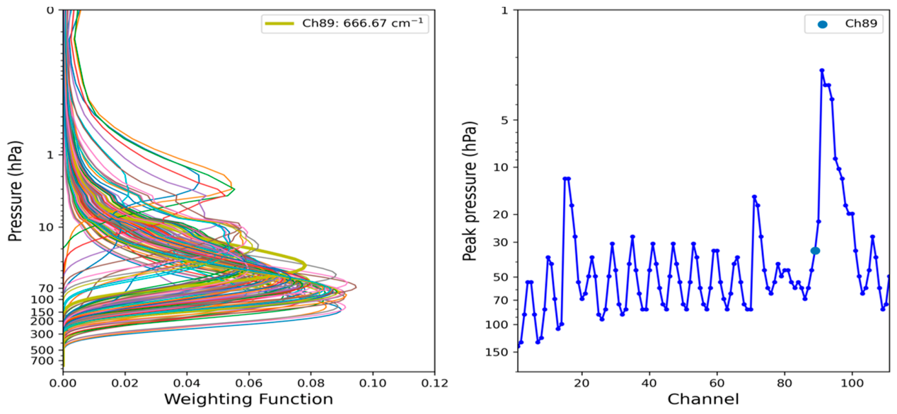
In this study, we focus on the CO₂ absorption band near 15 μm, corresponding to IASI wavenumbers from 645 to 672.5 cm⁻¹ (Ch1–111). Figure 2 illustrates the vertical sounding characteristics of the investigated IASI CO₂ absorption channels. The weighting functions, defined as $-{\displaystyle \frac{d{Tr}_k}{dln\left(p_k\right)}}$, span a broad range of atmospheric layers, with peak sensitivities varying from approximately 2–3 hPa in the upper stratosphere to about 150 hPa in the upper troposphere. This variation reflects the channel-dependent CO₂ absorption strength across the 15 μm band, enabling atmospheric temperature sounding over a wide range of altitudes. Channels located closer to strong CO₂ absorption regions generally exhibit higher-altitude sensitivity, whereas weaker absorption channels penetrate deeper into the atmosphere. The resulting distribution of weighting-function peak pressures demonstrates that the selected channels provide complementary vertical information throughout the upper troposphere and stratosphere, making this spectral region a demanding and informative testbed for evaluating the radiative-transfer consistency of the proposed LNN-LOD framework.

The CO₂ data applied here were downloaded from CAMS global inversion-optimized greenhouse gas fluxes and concentrations [23,24]. The targets (Y) of the training dataset used in this study are derived from CRTM version 3.0 simulations. The (X, g) shown in Equations (1) and (3) fully define the inputs to the radiative-transfer system. As a first step, ECMWF 91-level (ECMWF91L; [25]) forecast fields are spatially and temporally collocated with MetOp-B IASI BT observations. The matched atmospheric states, including vertical profiles of temperature/water vapor/O₃/CO₂, surface skin temperature, surface pressure, and associated sensor geometry, are then used as inputs to the CRTM forward model to generate physically IASI-consistent radiative-transfer outputs. The resulting CRTM simulations provide both the layer vertical optical depths,

$$∆{\tau }_k\in R^C,k=1,\dots ,L$$

and the corresponding brightness temperatures (BTs), where C = 111 denotes the number of spectral channels; L is the number of total vertical layers (=91). These simulated quantities serve as training targets (Y) for the CRTM-LNN, with both Δτ and BT treated as the primary learning targets. More details on the CRTM matching and simulation procedures can be found in [26,27].

CRTM-LNN is designed to approximate the mapping

(X, g) → Δτ → BT,

where the first stage, (X, g) → Δτ, is learned by the Liquid Neural Network, and the second stage, Δτ → BT, is computed analytically using the radiative equation.

To construct a robust and regime-balanced training dataset, data were collected across global land and ocean regions between 60°S and 60°N. To reduce potential contamination from high-level cirrus clouds, the dataset was screened using a brightness-temperature threshold of ∣O−B∣ < 5 K, where O denotes the IASI-observed BT and B denotes the corresponding CRTM-simulated BT [26,27]. This criterion served as a broad quality-control filter to remove gross radiance outliers and strongly cloud-contaminated scenes and to reduce, although not necessarily eliminate, residual thin-cloud contamination. The resulting dataset is therefore considered predominantly clear-sky, rather than strictly cloud-free.

To construct a balanced training dataset, prevent densely sampled atmospheric or viewing regimes from dominating the optimization, and ensure that rare or sparsely sampled conditions retain sufficient representation, the samples were stratified according to latitude, tropopause pressure, and viewing geometry. Specifically, latitude was divided into N_lat = 5 bins between 60°S and 60°N; tropopause pressure was separated into N_trop = 4 categories using boundaries at 100, 200, and 300 hPa; and viewing geometry was divided into N_sza = 10 bins based on the secant of the sensor zenith angle. This 5 × 4 × 10 = 200-regime stratification limits the overrepresentation of common conditions while preserving available samples from rare regimes, thereby promoting robust generalization across diverse atmospheric and observational conditions.

The complete dataset consists of 1,635,000 input–output pairs, (X, g) ⟷ (Δτ, BT), generated from 12 selected days over a year with global CRTM simulations in 2025, i.e., three days per month in January, April, July, and October. The complete dataset was randomly divided into training, validation, and test datasets containing 1,050,000, 135,000, and 450,000, respectively. This partitioning was intentionally adopted to reduce computational cost during training while retaining a held-out validation subset for internal assessment of predictive performance. Because these subsets are drawn from the same pooled dataset, results from the random test subset should not be interpreted as evidence of temporally independent generalization. Temporal generalization is assessed separately using data from six temporally independent days spanning November and December 2025 in this study.

Prior to model training, a logarithmic transform, log (Δτ + ϵ), is first applied to compress the large dynamic range of optical depth across channels and vertical layers, where ϵ is a small constant ($={10}^{-8})$ to ensure numerical stability. The transformed values are then standardized using channel mean and standard deviation, yielding a normalized representation that is well-suited for neural-network training. This preprocessing improves numerical conditioning, balances contributions from both weak and strong absorption regions, and stabilizes gradient propagation—particularly important in hyperspectral infrared bands where optical depth spans several orders of magnitude.

3. Model Training, Testing, and Validation

3.1. Model Training and Convergence Performance

This section evaluates the training performance of the proposed model using both validation and test datasets. The analysis focuses on brightness-temperature accuracy, optical-depth consistency, and computational efficiency relative to CRTM simulations. Metrics including RMSE, bias, and coefficient of determination (R²) are used to quantify model performance across channels, atmospheric regimes, and vertical structures. 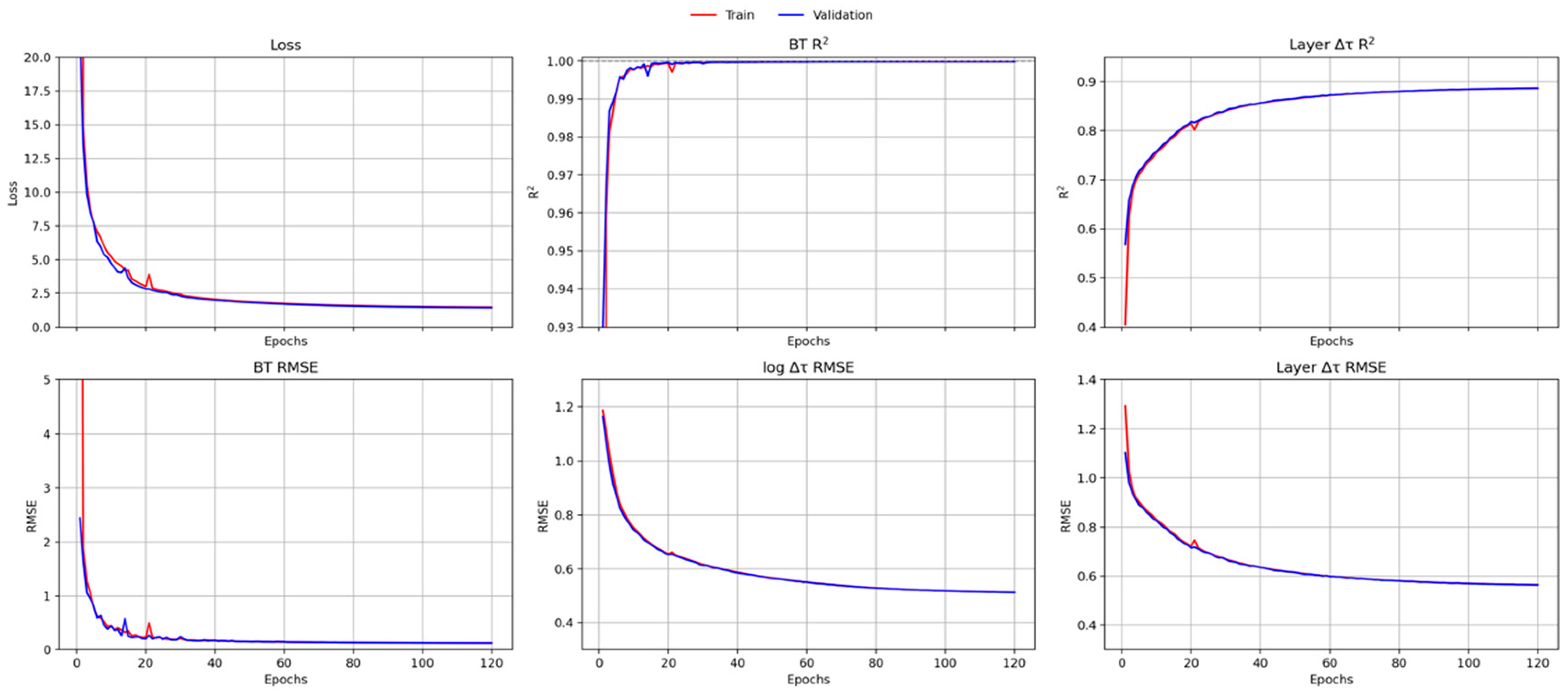Figure 3 demonstrates the training performance and convergence behavior of the proposed hybrid physics-informed CRTM-LNN over 120 training epochs. Training and validation losses remain highly consistent throughout optimization, indicating stable convergence and strong generalization capability without noticeable overfitting. The total loss decreases rapidly during the early training stage and gradually approaches a stable minimum. The BT prediction metrics exhibit exceptionally strong convergence characteristics. Both training and validation BT R² values quickly approach 1.0, while the corresponding BT RMSE decreases rapidly and stabilizes at a very low level, demonstrating highly accurate and robust BT prediction performance. The model also achieves strong learning capability for layer optical depth (Δτ) prediction. The layer Δτ R² increases steadily to approximately 0.90 for both training and validation datasets, while the corresponding RMSE decreases smoothly throughout training. Compared with BT prediction, Δτ convergence is more gradual, reflecting the higher complexity and nonlinearity of physically consistent layer optical-depth prediction. The log-transformed Δτ RMSE further demonstrates stable optimization across the full optical-depth dynamic range. The smooth monotonic decrease in both training and validation RMSE curves indicates that the model effectively learns both strong- and weak-absorption atmospheric layers without introducing significant optimization instability. Importantly, the close agreement between training and validation metrics across all panels confirms that the proposed physics-informed LNN-LOD framework achieves stable convergence behavior while maintaining strong physical consistency and predictive capability for both brightness temperature and optical-depth-related radiative-transfer variables.

3.2. Comprehensive Validation and Performance Assessment of the Emulator Using Independent Evaluation Datasets

To further evaluate the robustness and generalization capability of CRTM-LNN, additional independent datasets were selected from six separate days in late 2025, corresponding to 1 November 2025, 15 November 2025, 30 November 2025, 1 December 2025, 15 December 2025, and 31 December 2025. These datasets were completely independent of the training, validation, and testing datasets used during model development. Focusing on the latitude range of 60°S~60°N, the selected days span diverse temporal and atmospheric conditions, enabling comprehensive assessment of model stability, robustness, and radiative-transfer consistency under varying seasonal and geophysical environments. The emulator predictions were directly compared against CRTM simulations using channel-dependent brightness temperatures and other RT-related diagnostics, including transmittance, cumulative optical depth, and weighting functions, across all 111 IASI channels within the selected 15 µm CO₂ absorption band.

3.2.1. Output Evaluation: Brightness Temperature and Optical Depth Statistics

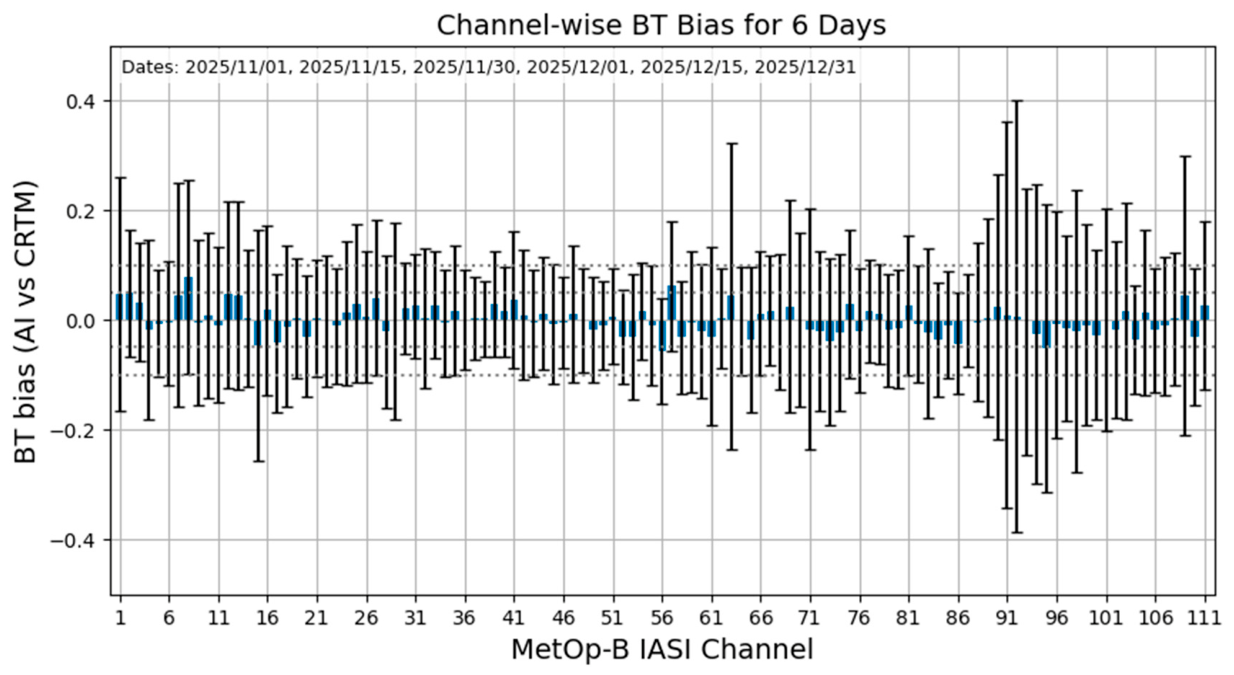
Figure 4 presents the IASI channel-dependent BT bias statistics between the CRTM-LNN results and CRTM reference simulations using six independent datasets from late 2025. Mean BT biases remain close to zero for nearly all channels, with most biases within approximately ±0.05 K, indicating minimal systematic error and excellent preservation of CRTM radiative-transfer characteristics. The channel standard deviations are generally below 0.2 K, demonstrating stable emulator performance across diverse atmospheric conditions. The absence of strong channel-dependent bias drift further highlights the spectral stability, robustness, and operational potential of the proposed CRTM-LNN for hyperspectral infrared radiative-transfer applications.

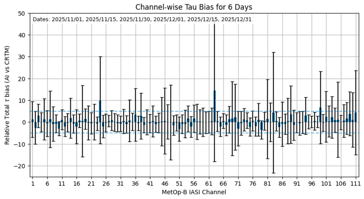
Because the CRTM-LNN directly predicts layer optical-depth increments (Δτ), it is important to evaluate optical-depth accuracy in addition to brightness temperatures. Figure 5 presents the channel-dependent relative bias (%) of vertically integrated optical depth between the emulator and CRTM for the same six independent evaluation days as above. Most channels exhibit small mean biases centered near zero (generally within ±2%), indicating that the emulator successfully reproduces the overall optical-depth structure learned from CRTM.

The channel-dependent standard deviations exhibit several localized peaks, indicating enhanced profile-to-profile sensitivity to atmospheric structure, viewing conditions, and absorption regimes for certain channels. Because the corresponding mean biases generally remain small, these peaks primarily reflect increased variability rather than persistent systematic errors. Overall, the results show good agreement between CRTM-LNN and CRTM across the atmospheric conditions represented in the evaluation dataset.

Importantly, balancing layer-level optical-depth fidelity with final radiometric accuracy is a deliberate design principle of the integrated CRTM-LNN framework. Layer-level Δτ errors do not contribute equally to the top-of-atmosphere radiance. Errors near the effective emitting region, where cumulative optical depth is typically of order unity, can strongly influence transmittance, weighting functions, and BTs. In contrast, errors in deeper layers beneath an already opaque region have little radiometric effect because their contributions are strongly attenuated. Therefore, accurate BTs alone do not fully characterize layer-level optical-depth fidelity. Conversely, uniformly emphasizing pointwise Δτ agreement across all layers could direct excessive model capacity toward radiatively inactive regions and compromise BT accuracy.

Accordingly, CRTM-LNN was designed to jointly constrain Δτ in normalized logarithmic and physical spaces, cumulative optical depth, and final BT through the analytic radiative-transfer pathway. This integrated training strategy balances local optical-property fidelity with end-to-end radiometric consistency rather than optimizing either objective in isolation. The cumulative optical depth, transmittance, and weighting functions receive greater emphasis in this study because they more directly quantify the radiative consequences of the remaining layer-level errors.

3.2.2. Evaluation of Model Performance on Cumulative Optical Depth, Transmittance, and Weighting Function

Although CRTM-LNN directly predicts layer optical-depth increments (Δτ), radiative-transfer calculations are ultimately governed by cumulative optical depth, atmospheric transmittance, and weighting functions. These quantities control atmospheric absorption, transmission, and radiance formation throughout the atmospheric column and therefore provide a more physically meaningful assessment of radiative-transfer consistency than individual layer optical depths alone.

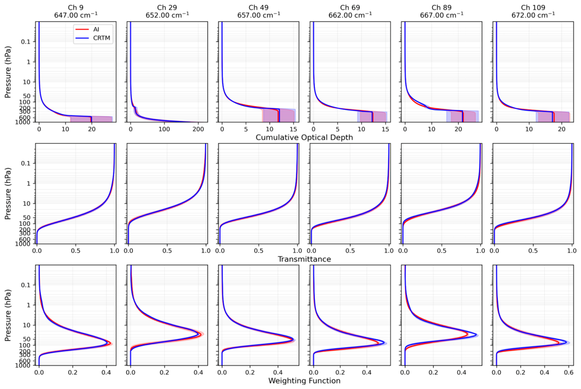
Figure 6 evaluates the vertical radiative-transfer behavior of the emulator using six representative IASI channels spanning the investigated 15 μm CO₂ absorption band. Here and in subsequent analyses, the weighting function is calculated using $wf=-{\displaystyle \frac{d{Tr}_k}{dln{(p}_k)}}$. Despite their substantially different absorption strengths and vertical sensitivities, the emulator accurately reproduces the cumulative optical depth, transmittance, and weighting-function profiles of CRTM. In particular, the magnitude, altitude, and spectral migration of weighting-function peaks are well preserved, indicating that the emulator successfully captures the fundamental radiative-transfer processes governing atmospheric radiance formation.

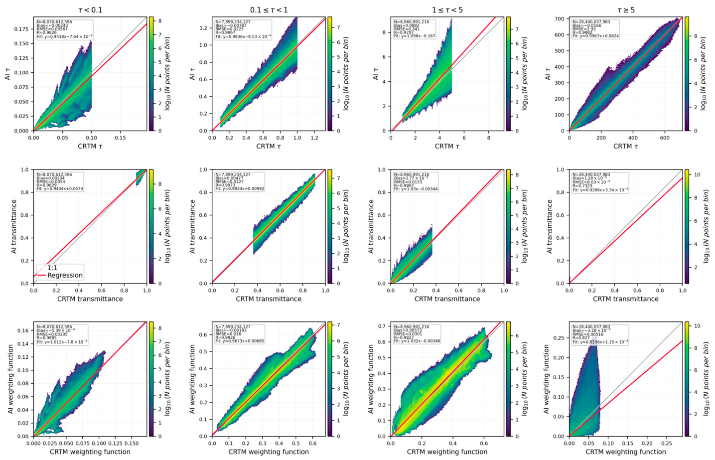
Figure 7 compares CRTM-LNN and CRTM cumulative optical depth, transmittance, and weighting functions over six evaluation days, stratified by the CRTM cumulative optical-depth regimes τ < 0.1, 0.1 ≤ τ < 1, 1 ≤ τ < 5, and τ ≥ 5. Overall, the high-density regions remain close to the 1:1 line, indicating good agreement across a broad range of absorption conditions. The strongest performance is obtained in the radiatively important intermediate regimes, 0.1 ≤ τ < 5, where transmittance is neither fully transparent nor saturated and optical-depth errors have the greatest influence on radiance formation.

For cumulative optical depth, CRTM-LNN performs well in the optically thin and moderately absorbing regimes. For τ < 0.1, the high R of 0.9826, the small negative bias of −0.00243, RMSE of 0.00567, and regression slope of 0.9418 indicate a slight underestimation of weak cumulative absorption. Agreement is strongest for 0.1 ≤ τ < 1, with R = 0.9967, RMSE = 0.0225, and a slope of 0.9836. The largest discrepancy occurs for 1 ≤ τ < 5, where the positive bias increases to 0.0882, the RMSE reaches 0.341, and the slope of 1.098 indicates increasing overestimation toward larger optical depths. For τ ≥ 5, the slope returns to nearly unity and R = 0.9982; although the RMSE is 2.93, this error is small relative to the very large optical-depth range and has limited radiative influence because the atmosphere is already nearly opaque.

The transmittance results are particularly strong. For all regimes with τ < 5, correlations exceed 0.98 and RMSE values remain below 0.016. Even in the 1 ≤ τ < 5 regime, where cumulative-optical-depth errors are largest, the transmittance bias is only 2.77 × 10⁻⁴, with an RMSE of 0.0153 and R = 0.9907. For τ ≥ 5, the correlation decreases to 0.7323 because both CRTM and CRTM-LNN transmittances are concentrated very close to zero, leaving little meaningful variance for correlation analysis. The extremely small bias of 1.28 × 10⁻⁵ and RMSE of 8.0 × 10⁻⁴ confirm that the absolute transmittance error in this opaque regime remains negligible.

The weighting functions also agree closely for τ < 5, with correlations of 0.9885, 0.9926, and 0.9827 across the first three regimes. The corresponding RMSE values are 0.00335, 0.0160, and 0.0301, respectively. The slight negative bias and regression slope below unity for 0.1 ≤ τ < 1 indicate modest underestimation of some layer contributions, whereas the positive bias and slope of 1.032 for 1 ≤ τ < 5 indicate slight overestimation in the stronger-transition regime. For τ ≥ 5, the lower correlation of 0.8270 and slope of 0.8336 reflect weaker agreement in the detailed weighting-function structure. Most values are near zero and therefore have little direct effect on TOA radiance; however, the broader scatter indicates that some layer contributions may be vertically misplaced when CRTM is already strongly opaque. Such localized differences may be more relevant to weighting function and Jacobian vertical localization than to final BT accuracy.

Overall, Figure 6 and Figure 7 show strong agreement between CRTM-LNN and CRTM in cumulative optical depth, transmittance, and weighting functions, particularly in the radiatively active range 0.1 ≤ τ < 5. The high correlations, small biases, and low RMSEs indicate that the emulator generally preserves the explicit optical-depth-to-radiance transformations represented by the clear-sky analytic solver. The main remaining discrepancies are the overestimation of cumulative optical depth for 1 ≤ τ < 5 and localized weighting-function differences for τ ≥ 5. Because the pooled statistics combine all channels and pressure levels, they may mask larger errors in specific transition channels or atmospheric layers; more detailed channel- and level-resolved analyses are therefore identified as future work.

3.2.3. Verification of Analytic Transmittance and Brightness-Temperature Jacobians

To verify the analytic derivative formulations in the radiative-transfer module, we evaluated the transmittance and brightness-temperature (BT) Jacobians with respect to layer optical-depth increments,

$$J_{Tr,\upsilon ,k}={\displaystyle \frac{\partial {Tr}_{\upsilon ,k}}{\partial {∆\tau }_j\left(\upsilon \right)}}=\{\begin{array}{cc}-{\displaystyle \frac{{Tr}_{\upsilon ,k}}{\mu }}& j\le k\\ 0& j>k\end{array}$$

(17)

$$J_{BT,\upsilon ,k}={\displaystyle \frac{\partial {BT}_{\upsilon }}{\partial {∆\tau }_k\left(\upsilon \right)}}=-{\displaystyle \frac{1}{\mu }}{\displaystyle \frac{(I_{\upsilon ,k+1}-B_{\upsilon }\left(T_k\right))e^{-\frac{{\tau }_k\left(\upsilon \right)}{\mu }}}{{\left(\frac{d{B}_{\upsilon }}{dT}\right)}_{{BT}_{\upsilon }}}}$$

(18)

where ${Tr}_k$ represents the transmittance shown in Equation (9), $I_{\upsilon ,k+1}$ is the radiance immediately below layer k. These Jacobians were calculated directly from the analytic radiative-transfer equations and did not require automatic differentiation. Because they are determined by optical depth, atmospheric temperature, and viewing geometry, their agreement with CRTM primarily verifies the analytic solver and derivative formulations rather than independently validating the learned atmospheric-state sensitivities. The learned sensitivity structure is evaluated separately using temperature and CO₂ Jacobians in the next sections.

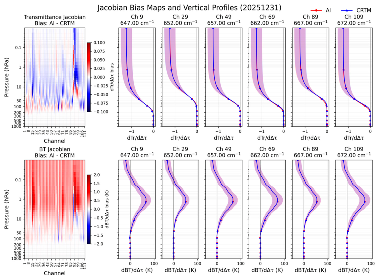
Transmittance and BT Jacobians derived from CRTM–LNN and CRTM were compared across all six temporally independent evaluation days. Figure 8 presents the comparison for 31 December 2025 as an illustrative example. The left panels show the global-mean channel- and pressure-dependent Jacobian bias distributions (CRTMLNN − CRTM) for all 111 IASI channels. Overall, both transmittance and BT Jacobians exhibit small residual biases throughout most of the atmospheric column. Similar to the optical-property diagnostics, the bias fields display alternating positive and negative patterns rather than systematic errors, with the largest differences confined mainly to the rapid-transition CO₂ absorption channels (approximately Ch16 and Ch89–Ch100), where vertical radiative sensitivity changes most rapidly.

The right panels compare vertical Jacobian profiles for six representative channels spanning the 15 μm CO₂ absorption band. The emulator accurately reproduces the magnitude, peak location, and overall vertical structure of both transmittance and BT Jacobians across channels with substantially different absorption strengths. Although small, localized differences remain near the sensitivity maxima, the overall agreement is excellent.

These Jacobian comparisons primarily support the consistency of the analytic solver and its derivatives, rather than independently validating learned atmospheric-state sensitivities. The latter are assessed separately through temperature- and CO₂-Jacobian comparisons, subject to the limitations discussed in the corresponding subsections.

In addition, the largest biases remain concentrated near Ch16 and Ch89–Ch100, where the weighting-function peaks shift rapidly over a broad vertical range (Figure 2). These transition channels sample substantially different atmospheric layers within a relatively narrow spectral interval, making them particularly sensitive to small errors in the vertical optical-depth structure. Consequently, even minor inaccuracies in the vertical distribution of absorption can be amplified into larger transmittance errors in these transition regions. This behavior also suggests that although the transition channels remain the most challenging, this behavior suggests that the proposed CRTM-LNN captures the underlying continuous radiative-transfer dynamics to a considerable extent, preserving the physical structure of atmospheric absorption rather than merely learning a global input–output mapping.

3.2.4. Evaluation of Model Performance on the Jacobian Terms from Automatic Differentiation

The proposed physics-informed LNN-LOD framework can directly generate physically meaningful Jacobians and radiative sensitivities without requiring a separate Jacobian network, tangent-linear model, or adjoint model. Because the predicted layer optical depths are coupled with a fully analytic and differentiable radiative-transfer solver, the entire framework remains end-to-end differentiable. Consequently, radiative sensitivities with respect to atmospheric temperature, trace gases, optical depth, and other state variables can be obtained efficiently through automatic differentiation of the trained model.

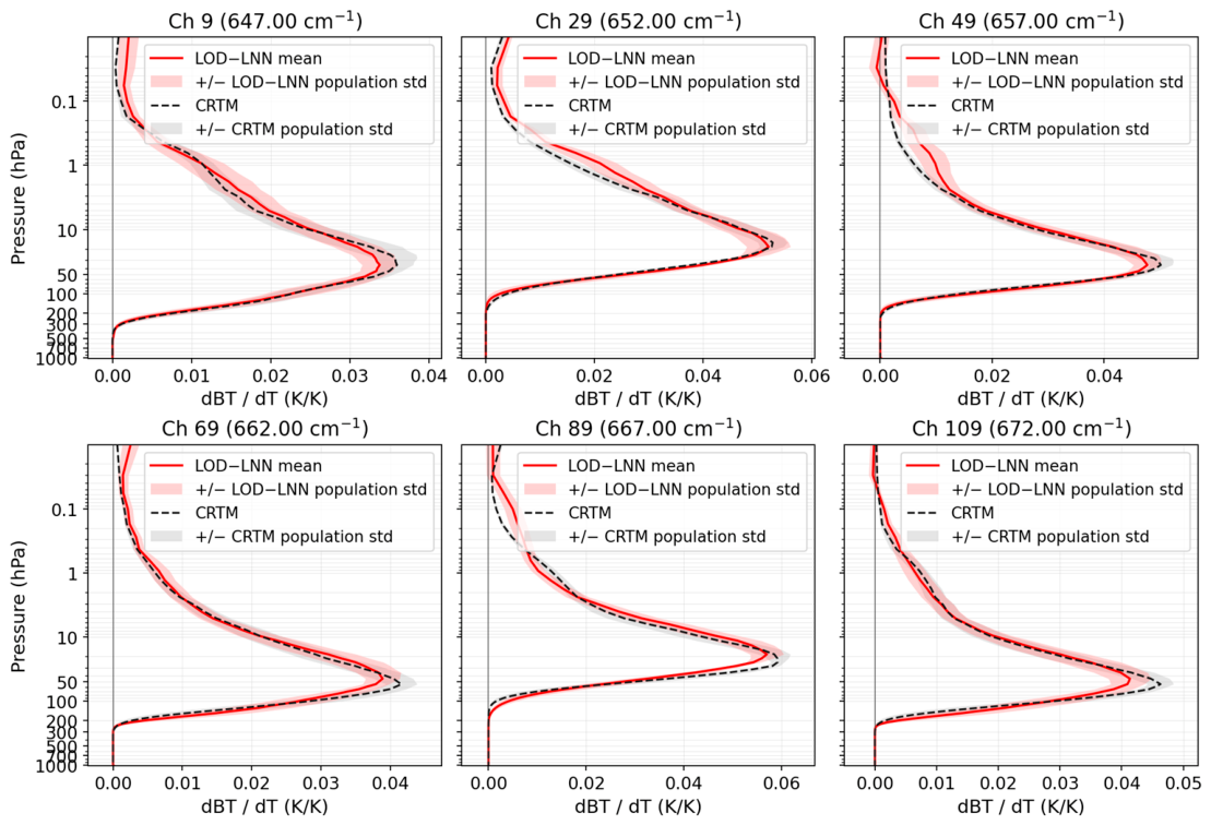
The selected IASI channels (Ch1–Ch111) lie within the 15 μm CO₂ absorption band and exhibit relatively weak sensitivity to atmospheric water vapor and most other atmospheric constituents. Therefore, this study focuses on the temperature Jacobian (∂BT/∂T), which represents the dominant radiative sensitivity for these channels. Figure 9 compares the temperature Jacobians produced by CRTM-LNN with the corresponding CRTM K-matrix Jacobians for six representative channels on 31 December 2025. Overall, the CRTM-LNN Jacobians successfully reproduce the vertical sensitivity structure of the CRTM, including the dominant upper-tropospheric and lower-stratospheric sensitivity peaks and their systematic altitude shifts across the spectral band. The good agreement in both the location and magnitude of the primary sensitivity maxima indicates that the model has learned the dominant radiative-response characteristics of atmospheric temperature perturbations. The relatively narrow uncertainty envelopes further demonstrate stable and robust Jacobian behavior across the independent evaluation dataset.

Some differences remain in the detailed shape and amplitude of the sensitivity peaks, particularly in channels exhibiting sharp vertical sensitivity gradients. In these regions, small differences in the predicted optical-depth, transmittance, or weighting-function structures can be amplified in the resulting Jacobians. Because the Jacobians are obtained through automatic differentiation of the complete physics-informed framework, the remaining Jacobian differences primarily reflect residual inaccuracies in the predicted optical-depth structure rather than deficiencies in the differentiation procedure itself.

Unlike brightness temperatures, derivative quantities are inherently more sensitive to local approximation errors in the neural representation. Consequently, small optical-depth errors may have only a minor impact on forward radiance simulations but become amplified in the corresponding Jacobians. This effect is particularly pronounced for weaker sensitivity terms associated with other atmospheric variables, such as water vapor and ozone concentration, whose Jacobians are substantially smaller than the dominant temperature Jacobian (please see some discussions in Section 3.2.6). As a result, these weaker sensitivities are inherently more difficult to learn accurately, although their impact on overall radiative-transfer accuracy and atmospheric sounding performance is generally limited. Nevertheless, the overall agreement demonstrates that the emulator successfully preserves the dominant radiative sensitivities governing the 15 μm CO₂ band. This result is particularly encouraging because temperature Jacobians constitute the primary sensitivity term for atmospheric sounding, retrieval, and data-assimilation applications within this spectral region.

In addition, close agreement in the total temperature Jacobian may partly reflect the analytically prescribed Planck-source contribution and therefore may not, by itself, demonstrate that the temperature dependence of layer optical depth has been fully learned. Further analysis on Jacobian metrics will be presented in the following Section 3.2.5 and Section 3.2.6.

3.2.5. An Ablation Study on the Loss Term ${\mathcal{L}}_{vs}$

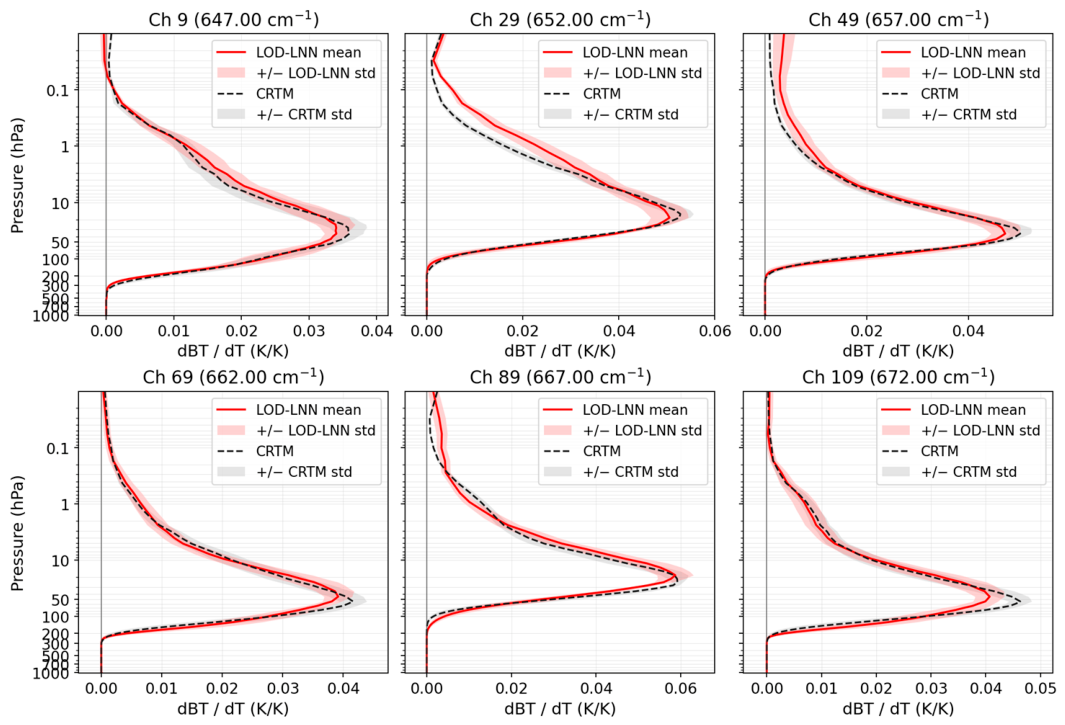
In this study, we conducted an ablation study to check the contribution of the vertical-smoothing loss ${\mathcal{L}}_{vs}$. In this new experiment, we set ${\omega }_{vs}=0.0$. Figure 10 is the same as Figure 9, except for no_Lvs. The two sets of results are highly similar across all six representative channels. The mean Jacobian profiles retain nearly identical vertical shapes, peak pressures, peak magnitudes, and sensitivity ranges, and both configurations reproduce the overall CRTM vertical structure well. The profile-to-profile standard-deviation envelopes are also comparable, with no consistent reduction in variability after removing ${\mathcal{L}}_{vs}$. Small differences are visible at some upper-atmospheric levels and near the Jacobian peaks, but they are minor and do not show a systematic improvement across channels.

The channel-dependent discrepancies relative to CRTM also remain largely unchanged. For example, both configurations show slight underestimation of the Jacobian peaks for several channels, including Ch9, Ch49, Ch69, and Ch109, while the modest upper-atmospheric differences in Ch29, Ch49, and Ch89 persist after introducing the smoothing term. Thus, ${\mathcal{L}}_{vs}$ does not materially correct the remaining peak-amplitude or vertical-localization differences. More importantly, the model trained without ${\mathcal{L}}_{vs}$ already produces smooth and vertically coherent Jacobian profiles, with no substantial increase in spurious layer-to-layer oscillations.

This ablation indicates that ${\mathcal{L}}_{vs}$ functions primarily as a weak regularizer that may suppress minor local fluctuations without controlling the main Jacobian structure. The overall vertical coherence therefore appears to arise mainly from the integrated CRTM-LNN design—including the LNN-LOD layer-by-layer state evolution, direct supervision of layer optical-depth increments, cumulative optical-depth constraints, and analytic radiative-transfer coupling—rather than from the explicit smoothing penalty alone.

Table 6. Comparison of temperature-Jacobian metrics from CRTM-LNN models trained with and without the vertical-smoothing loss ${\mathcal{L}}_{vs}$. Spatial mean Jacobian profiles and their ±1 standard-deviation envelopes over 872,532 profiles are shown for 31 December 2025.

Variable		Jacobian-Profile RMSE	Jacobian-Profile Corr.	Abs. Peak-p Error (hPa)	Abs. Centroid-p Error (hPa)	Vertical-Roughness Mismatch
Ch9	$\mathrm{with}{\mathcal{L}}_{vs}$	0.00223711 ± 0.000985672	0.984591 ± 0.0141226	7.54311 ± 6.78795	4.37183 ± 3.30724	0.160508 ± 0.132905
	$\mathrm{without}{\mathcal{L}}_{vs}$	0.00212646 ± 0.000851163	0.985778 ± 0.0118809	7.89518 ± 7.53589	3.91791 ± 2.53039	0.165107 ± 0.139135
Ch29	$\mathrm{with}{\mathcal{L}}_{vs}$	0.00250732 ± 0.000972709	0.989522 ± 0.00841641	2.42193 ± 2.46676	1.76841 ± 1.13258	0.0886009 ± 0.0218551
	$\mathrm{without}{\mathcal{L}}_{vs}$	0.0029594 ± 0.000884596	0.985856 ± 0.00844156	2.62272 ± 2.62163	2.1879 ± 1.35922	0.0890436 ± 0.0213407
Ch49	$\mathrm{with}{\mathcal{L}}_{vs}$	0.00270945 ± 0.00125519	0.984737 ± 0.0142031	5.27324 ± 4.43166	3.58915 ± 2.52585	5.56933 ± 8.28571
	$\mathrm{without}{\mathcal{L}}_{vs}$	0.00274916 ± 0.00123639	0.984587 ± 0.0142727	5.50563 ± 4.48221	3.72836 ± 2.43326	4.39196 ± 6.3135
Ch69	$\mathrm{with}{\mathcal{L}}_{vs}$	0.00299729 ± 0.00132287	0.97566 ± 0.0209765	10.9728 ± 7.68454	4.62419 ± 3.38318	2.66856 ± 6.81185
	$\mathrm{without}{\mathcal{L}}_{vs}$	0.00294401 ± 0.00133347	0.976077 ± 0.021235	11.0448 ± 7.54553	5.19631 ± 3.52385	1.80343 ± 4.01739
Ch89	$\mathrm{with}{\mathcal{L}}_{vs}$	0.00333181 ± 0.00111179	0.982667 ± 0.0131838	5.26292 ± 3.68911	1.7859 ± 1.2784	0.128358 ± 0.0295561
	$\mathrm{without}{\mathcal{L}}_{vs}$	0.00328286 ± 0.00122079	0.982605 ± 0.0137023	5.0807 ± 3.6108	1.94445 ± 1.36945	0.132048 ± 0.0495752
Ch109	$\mathrm{with}{\mathcal{L}}_{vs}$	0.0036324 ± 0.00157051	0.968872 ± 0.0258975	9.38379 ± 6.91835	5.01093 ± 3.61691	0.31688 ± 0.360008
	$\mathrm{without}{\mathcal{L}}_{vs}$	0.00370933 ± 0.00142853	0.968194 ± 0.024036	10.8724 ± 7.40961	5.46791 ± 3.69272	0.287902 ± 0.200308

further compares the spatial mean Jacobian metrics with their spatial standard deviations (STDs) between the CRTM-LNN with and without ${\mathcal{L}}_{vs}$ using the data on 31 December 2025. Five complementary diagnostics were used to evaluate the vertical fidelity of the atmospheric-state Jacobians. For each atmospheric variable, spectral channel, and matched profile, the CRTM-LNN and CRTM Jacobian vectors were compared across all 91 atmospheric layers. The profile-level diagnostics included Jacobian-profile RMSE and correlation, the absolute peak-pressure error, the absolute centroid-pressure error, and the vertical-roughness mismatch. For each channel, variable, and atmospheric profile, the Jacobian RMSE quantifies the overall magnitude of the layer-by-layer differences, with smaller values indicating closer agreement, while the Pearson correlation coefficient measures the similarity of the vertical-profile shape, with values approaching unity indicating strong structural agreement. The peak pressure was defined as the pressure level at which the absolute Jacobian magnitude was largest. The centroid pressure is calculated using the absolute Jacobian magnitude in log-pressure coordinates:

$$p_{centroid}^{\left(J\right)}={10}^{{\displaystyle \frac{\sum _k\left|J_{\upsilon ,x,k}\right|{log}_{10}{p}_k}{\sum _k\left|J_{\upsilon ,x,k}\right|}}}.$$

Peak- and centroid-pressure errors are reported as the absolute difference between the AI-derived pressures and the corresponding CRTM reference values. These metrics quantify the magnitude of the displacement in pressure coordinates, with smaller values indicating closer agreement with the reference Jacobian locations. Vertical roughness was quantified by the root-mean-square second derivative of the Jacobian with respect to log₁₀(p), while the roughness-mismatch RMSE measured the difference between the AI and CRTM Jacobian curvatures. Thus, peak pressure characterizes the location of maximum sensitivity, centroid pressure characterizes the overall vertical localization of the radiance information, and roughness characterizes the smoothness and small-scale vertical structure of the Jacobian profile. Finally, for each channel, the spatial mean and standard deviation of each profile-level metric were calculated over the same 872,532 matched profiles on 31 December 2025.

Table 6 shows that with ${\mathcal{L}}_{vs}$, CRTM-LNN maintains strong temperature-Jacobian fidelity across the six channels, with correlations of 0.969–0.990, RMSEs of 2.24 × 10⁻³–3.63 × 10⁻³, absolute peak-pressure errors of 2.42–10.97 hPa, and absolute centroid-pressure errors of 1.77–5.01 hPa. Comparisons with the configuration without ${\mathcal{L}}_{vs}$ present generally small and channel-dependent differences: ${\mathcal{L}}_{vs}$ modestly improves several RMSE, correlation, and vertical-localization metrics, particularly for Ch29 and Ch109, but does not improve every metric. Notably, the model without ${\mathcal{L}}_{vs}$ produces smaller roughness mismatches for Ch49 (4.39 versus 5.57) and Ch69 (1.80 versus 2.67). Overall, ${\mathcal{L}}_{vs}$ acts mainly as a weak supplementary regularizer rather than the primary source of the smooth and vertically coherent Jacobians generated by CRTM-LNN.

3.2.6. Comparison with MLP Model Focusing on BT Jacobians Only

To provide a supporting baseline for evaluating the Jacobian fidelity of the complete CRTM-LNN framework, a conventional CRTM-MLP emulator was developed using the same training dataset and input preprocessing [28]. The MLP contains 460 input features$-\{x_k,g\}$ (i.e., Equations (1) and (3)), followed by three fully connected hidden layers with 512, 256, and 256 neurons, respectively. Its output layer contains 10,212 elements, jointly representing the 111-channel brightness temperatures and the corresponding (111 × 91) layer optical-depth increments. As in CRTM-LNN, the optical-depth targets were first transformed using log (Δτ + ϵ) to compress their large dynamic range and improve numerical stability, after which both the input variables and target outputs were normalized before training. The MLP was trained using the same training dataset as the CRTM-LNN. The training is configured for up to 100 epochs using mean squared error, the Adam optimizer, a batch size of 2048, and mixed precision. The initial learning rate of 10⁻³ is halved every 15 epochs. The best validation-loss checkpoint is retained. Because the CRTM-MLP and CRTM-LNN differ not only in neural architecture but also in their vertical state representation, radiative-transfer coupling, and training constraints, this comparison should be interpreted as an evaluation of two complete emulator designs rather than as a strict isolation of the network architecture alone. The reported CRTM–LNN and CRTM–MLP results are based on a single training realization for each model.

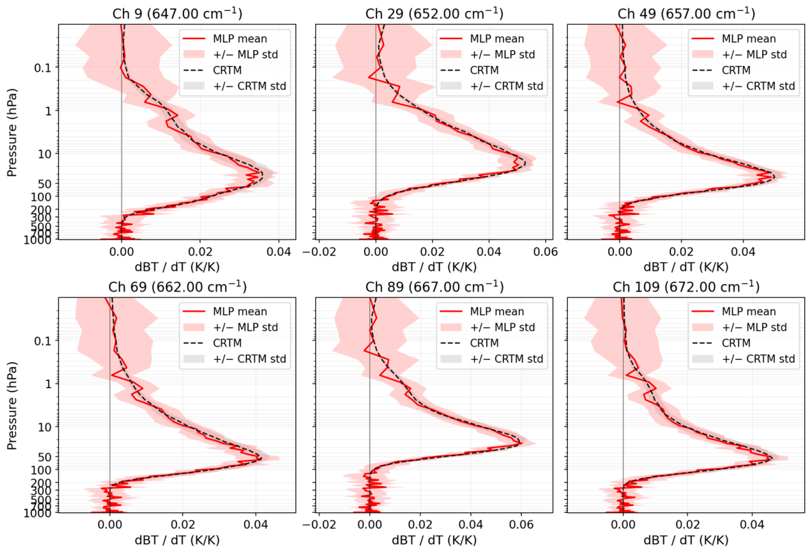
Figure 11 presents the temperature Jacobians generated by the conventional CRTM-MLP emulator. Compared with the CRTM-LNN results in Figure 9, the two models exhibit substantially different vertical-sensitivity characteristics. CRTM-LNN more closely reproduces the CRTM reference profiles throughout the atmospheric column, yielding smoother vertical structures and profile-to-profile standard-deviation envelopes comparable to those of CRTM. In contrast, CRTM-MLP shows substantially greater variability at pressures below approximately 1 hPa and pronounced layer-to-layer oscillations in both strong- and weak-sensitivity regions. These oscillations are particularly evident between approximately 200 and 1000 hPa, where accurate vertical attribution of radiance information is important for numerical weather prediction.

Similar oscillatory behavior in low-sensitivity regions has been reported for fully connected CRTM emulators by Liang et al. [13], indicating that high forward-model accuracy does not necessarily guarantee smooth and vertically coherent radiative sensitivities. Such oscillations may introduce spurious observation sensitivities, misattribute radiance information to incorrect atmospheric layers, and adversely affect variational data assimilation and forecast initialization. By retaining the explicit pathway from layer optical depth to radiance, CRTM-LNN substantially suppresses these nonphysical oscillations and produces Jacobians that more closely follow the vertical structure of the CRTM reference. Moreover, the analysis in Section 3.2.5 shows that the configurations trained with and without ${\mathcal{L}}_{vs}$ yield generally similar Jacobian metrics. Therefore, the improved smoothness and vertical coherence of CRTM-LNN relative to the MLP baseline cannot be attributed primarily to the vertical-smoothing loss; instead, they reflect the combined effects of the LNN-LOD vertical state evolution, supervised optical-depth prediction, and analytic radiative-transfer coupling.

Table 7. Comparison of temperature-Jacobian metrics between CRTM-LNN and CRTM-MLP. Spatial mean Jacobian profiles and their ±1 standard-deviation envelopes over 872,532 profiles are shown for 31 December 2025. Note: the CRTM-LNN results are identical to those reported in Table 6 for the configuration with the vertical-smoothing loss ${\mathcal{L}}_{vs}$; they are repeated here to facilitate direct comparison.

Variable		Jacobian-Profile RMSE	Jacobian-Profile Corr.	Abs. Peak-p Error (hPa)	Abs. Centroid-p Error (hPa)	Vertical-Roughness Mismatch
		Temperature Jacobian Metrics
Ch9	CRTM-LNN	0.00223711 ± 0.000985672	0.984591 ± 0.0141226	7.54311 ± 6.78795	4.37183 ± 3.30724	0.160508 ± 0.132905
	CRTM-MLP	0.00546768 ± 0.00125965	0.914337 ± 0.0398085	12.9905 ± 12.9287	5.87686 ± 4.36475	335.025 ± 112.859
Ch29	CRTM-LNN	0.00250732 ± 0.000972709	0.989522 ± 0.00841641	2.42193 ± 2.46676	1.76841 ± 1.13258	0.0886009 ± 0.0218551
	CRTM-MLP	0.00693719 ± 0.00172388	0.92073 ± 0.0405987	5.24675 ± 3.73189	7.3 ± 3.44382	439.238 ± 245.62
Ch49	CRTM-LNN	0.00270945 ± 0.00125519	0.984737 ± 0.0142031	5.27324 ± 4.43166	3.58915 ± 2.52585	5.56933 ± 8.28571
	CRTM-MLP	0.00620718 ± 0.0014786	0.92938 ± 0.0354335	7.3511 ± 5.7945	6.88172 ± 4.5124	305.002 ± 149.202
Ch69	CRTM-LNN	0.00299729 ± 0.00132287	0.97566 ± 0.0209765	10.9728 ± 7.68454	4.62419 ± 3.38318	2.66856 ± 6.81185
	CRTM-MLP	0.00570007 ± 0.0013881	0.924221 ± 0.0374498	11.9594 ± 9.76038	6.86477 ± 4.98645	294.203 ± 106.069
Ch89	CRTM-LNN	0.00333181 ± 0.00111179	0.982667 ± 0.0131838	5.26292 ± 3.68911	1.7859 ± 1.2784	0.128358 ± 0.0295561
	CRTM-MLP	0.0072581 ± 0.00168843	0.924161 ± 0.0361681	4.54453 ± 4.22487	8.16641 ± 4.01981	421.151 ± 234.197
Ch109	CRTM-LNN	0.0036324 ± 0.00157051	0.968872 ± 0.0258975	9.38379 ± 6.91835	5.01093 ± 3.61691	0.31688 ± 0.360008
	CRTM-MLP	0.00599941 ± 0.00149055	0.926278 ± 0.0377427	10.4746 ± 8.88207	6.8062 ± 4.97771	292.211 ± 107.95

further compares the mean temperature Jacobian metrics between the CRTM-LNN and CRTM-MLP using the data of 2025/12/31. This table shows that CRTM- LNN generally reproduces the CRTM temperature Jacobians more accurately than the CRTM-MLP baseline across the six selected channels. CRTM-LNN yields lower RMSEs for every channel, ranging from 2.24 × 10⁻³ to 3.63 × 10⁻³, compared with 5.47 × 10⁻³ to 7.26 × 10⁻³ for CRTM-MLP. Its correlations are also consistently higher, ranging from 0.969 to 0.990, whereas the MLP correlations range from 0.914 to 0.929. Averaged over the six channels, CRTM-LNN reduces the Jacobian RMSE by approximately 54% and increases the correlation by about 0.058.

The vertical-localization metrics also generally favor CRTM-LNN. Its centroid-pressure errors are smaller for all six channels, with the largest improvements occurring for Ch29 and Ch89. Peak-pressure errors are reduced for five of the six channels, although the improvement for Ch69 is modest and CRTM-MLP performs slightly better for Ch89, with errors of 4.54 hPa for MLP and 5.26 hPa for LNN. These results indicate that CRTM-LNN better preserves the overall center of the vertical sensitivity profile, while its advantage in locating the single maximum is less uniform. The relatively large standard deviations of some pressure-error metrics also indicate substantial profile-to-profile variability and should be considered when interpreting the mean differences.

The clearest difference occurs in vertical-roughness mismatch. CRTM-LNN produces substantially smaller values for every channel, whereas the MLP values range from approximately 292 to 439, indicating pronounced disagreement with the CRTM vertical curvature structure. The LNN roughness mismatch remains below 0.32 for Ch9, Ch29, Ch89, and Ch109, although larger values and variability occur for Ch49 and Ch69. Nevertheless, even for these two channels, the LNN mismatches of 5.57 and 2.67 remain far below the corresponding MLP values of 305.00 and 294.20. Overall, the table supports improved Jacobian magnitude, correlation, vertical localization, and especially vertical coherence for the integrated CRTM-LNN framework. Because the two baselines differ in prediction pathway and model design, however, these results should be interpreted as a comparison of the complete emulator frameworks rather than as evidence that the LNN architecture alone causes every improvement.

Table 8. The same as Table 7, except for CO₂-Jacobian metrics. Spatial mean Jacobian profiles and their ±1 standard-deviation envelopes over 872,532 profiles are shown for 31 December 2025.

Variable		RMSE	Corr.	Abs. Peak-p Error (hPa)	Abs. Centroid-p Error (hPa)	Vertical-Roughness Mismatch
		CO2-Jacobian Metrics
Ch9	CRTM-LNN	0.00246902 ± 0.00115106	0.0830301 ± 0.349024	13.803 ± 26.432	9.41494 ± 5.27594	0.0524791 ± 0.0354677
	CRTM-MLP	0.0254032 ± 0.00910398	0.0182369 ± 0.0579377	8.6825 ± 19.6441	9.74681 ± 5.18589	84.8172 ± 56.1502
Ch29	CRTM-LNN	0.00274155 ± 0.000959467	0.00491019 ± 0.281853	3.37633 ± 2.31464	4.28346 ± 0.9237	0.0250078 ± 0.00956602
	CRTM-MLP	0.038818 ± 0.0115781	0.0243181 ± 0.059083	3.57686 ± 2.325	2.04808 ± 1.13062	132.493 ± 82.6635
Ch49	CRTM-LNN	0.00310533 ± 0.0011706	0.226348 ± 0.132141	65.627 ± 98.8153	8.65375 ± 5.13146	0.137944 ± 0.21438
	CRTM-MLP	0.0330502 ± 0.0122134	0.0143318 ± 0.0526811	65.6074 ± 98.8023	5.99655 ± 5.06246	118.576 ± 66.7329
Ch69	CRTM-LNN	0.00621823 ± 0.00845807	0.210773 ± 0.147405	138.408 ± 145.814	20.9861 ± 31.078	3.26426 ± 7.9748
	CRTM-MLP	0.0278353 ± 0.0104504	0.013494 ± 0.0572386	138.458 ± 146.766	19.1202 ± 31.0265	94.1979 ± 55.2835
Ch89	CRTM-LNN	0.0131434 ± 0.00384192	0.212436 ± 0.0607536	6.74931 ± 28.6453	4.99388 ± 1.59905	0.0678939 ± 0.0839954
	CRTM-MLP	0.0422816 ± 0.0140194	0.0227821 ± 0.0539093	6.70441 ± 28.6484	2.6712 ± 1.581	144.299 ± 81.8401
Ch109	CRTM-LNN	0.0034777 ± 0.00162339	0.155501 ± 0.121595	71.0989 ± 121.412	10.2017 ± 9.80429	0.381067 ± 0.909979
	CRTM-MLP	0.0273099 ± 0.00985015	0.0205563 ± 0.0532455	70.0998 ± 122.125	8.57331 ± 9.67578	97.7544 ± 57.2827

is the same as Table 7, except for CO₂ Jacobians. This table shows that CRTM-LNN provides a clear improvement over CRTM-MLP in reproducing the magnitude and vertical smoothness of the CO₂ Jacobians. Across the six selected channels, CRTM-LNN reduces the Jacobian RMSE by approximately 69–93% and produces substantially smaller vertical-roughness mismatches. Its correlations are also generally higher than those of CRTM-MLP, except for Ch29, where both correlations remain close to zero. Nevertheless, accurate CO₂-Jacobian representation remains challenging: the CRTM-LNN correlations are still relatively low (0.005–0.226), peak-pressure errors remain comparable to those of CRTM-MLP and exceed 65–138 hPa for several channels, and centroid-pressure errors are not consistently improved. The large spatial standard deviations further indicate considerable profile-to-profile variability in the vertical localization of the CO₂ sensitivities. Unlike temperature Jacobians, CO₂ Jacobians do not benefit from a direct Planck-source contribution and depend primarily on the learned sensitivity of layer optical depth to CO₂. In addition, the CO₂ cap (approximately 366~400 ppmv) applied in the current CRTM configuration compresses the CO₂ variability represented in the training targets, thereby limiting the range of CO₂-dependent absorption responses available to the AI model and likely contributing to the reduced Jacobian correlation and vertical-localization accuracy.

Future work should therefore incorporate broader physically realistic CO₂ variability, targeted CO₂ perturbations, and gas- or layer-dependent sensitivity constraints to improve CO₂-Jacobian fidelity.

Above all, the low CO₂-Jacobian correlations (0.005 to 0.226; Table 8) are consistent with weakly constrained optical-depth sensitivities to CO₂, emphasizing that agreement in the total temperature Jacobian should not be interpreted as validation of all learned optical-depth sensitivities. Nevertheless, CRTM–LNN achieves consistently higher temperature-Jacobian correlations with the reference CRTM calculations (0.969–0.990) than CRTM–MLP (0.914–0.929), demonstrating improved agreement in the vertical structure of temperature sensitivities across the evaluated channels. This comparative advantage supports the ability of CRTM–LNN to reproduce the overall temperature response more faithfully.

3.3. O-B ∆BT Analysis

Comparisons with CRTM directly assess emulator fidelity, while comparisons with IASI observations provide a complementary assessment of observation–simulation consistency, as the |O−B_CRTM∣ < 5 K screening was used for the training dataset generation. Accordingly, O–B (observation minus background) diagnostics are examined to determine whether CRTM–LNN preserves the observational agreement achieved by the reference CRTM. Here, O denotes the observed brightness temperature, and B denotes the corresponding CRTM- or emulator-simulated brightness temperature. Comparing their O–B statistics provides an application-oriented assessment of the emulator’s ability to reproduce the reference model’s radiometric behavior relevant to radiance monitoring, retrieval, and data assimilation.

While comparisons against CRTM provide a direct assessment of emulator fidelity, they do not fully demonstrate whether the emulator preserves the radiometric characteristics observed in real satellite measurements. Therefore, O–B (observation minus background) diagnostics are further examined as a complementary observation-based assessment. O–B statistics are widely used in satellite calibration, validation, and data assimilation because they directly quantify the consistency between observations and model-simulated radiances. By comparing O–B values computed using emulator-generated radiances and CRTM-generated radiances, it is possible to determine whether the emulator reproduces not only the CRTM forward calculations but also the observation-based radiometric behavior relevant to operational applications. Consequently, agreement in O–B statistics provides a more practical and application-oriented validation of the emulator’s performance, demonstrating its ability to maintain the observational consistency required for radiance monitoring, retrieval, and data-assimilation systems.

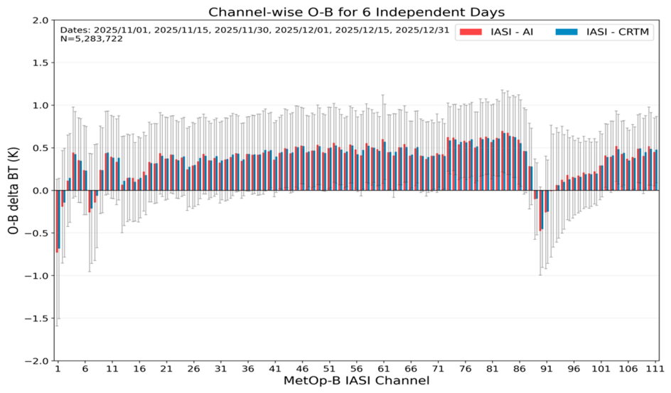
Figure 12 compares channel-dependent O–B BT statistics derived from the CRTM-LNN and CRTM across six independent evaluation days. Overall, the emulator closely reproduces the O–B characteristics of CRTM throughout the entire 15 μm CO₂ absorption band, with nearly identical mean values and variability across all 111 channels. Both datasets exhibit consistent channel-dependent behavior, including the stronger positive O–B values near the center of the CO₂ absorption band and the negative O–B values observed in several strongly absorbing channels. The differences between the emulator and CRTM are generally small relative to the corresponding standard deviations, indicating that the emulator successfully preserves the radiometric characteristics represented by the CRTM forward model. The analysis includes approximately 5.28 million independent observations spanning a wide range of atmospheric, geographical, and seasonal conditions. The close agreement further demonstrates the robustness and generalization capability of CRTM-LNN under diverse atmospheric and observational conditions.

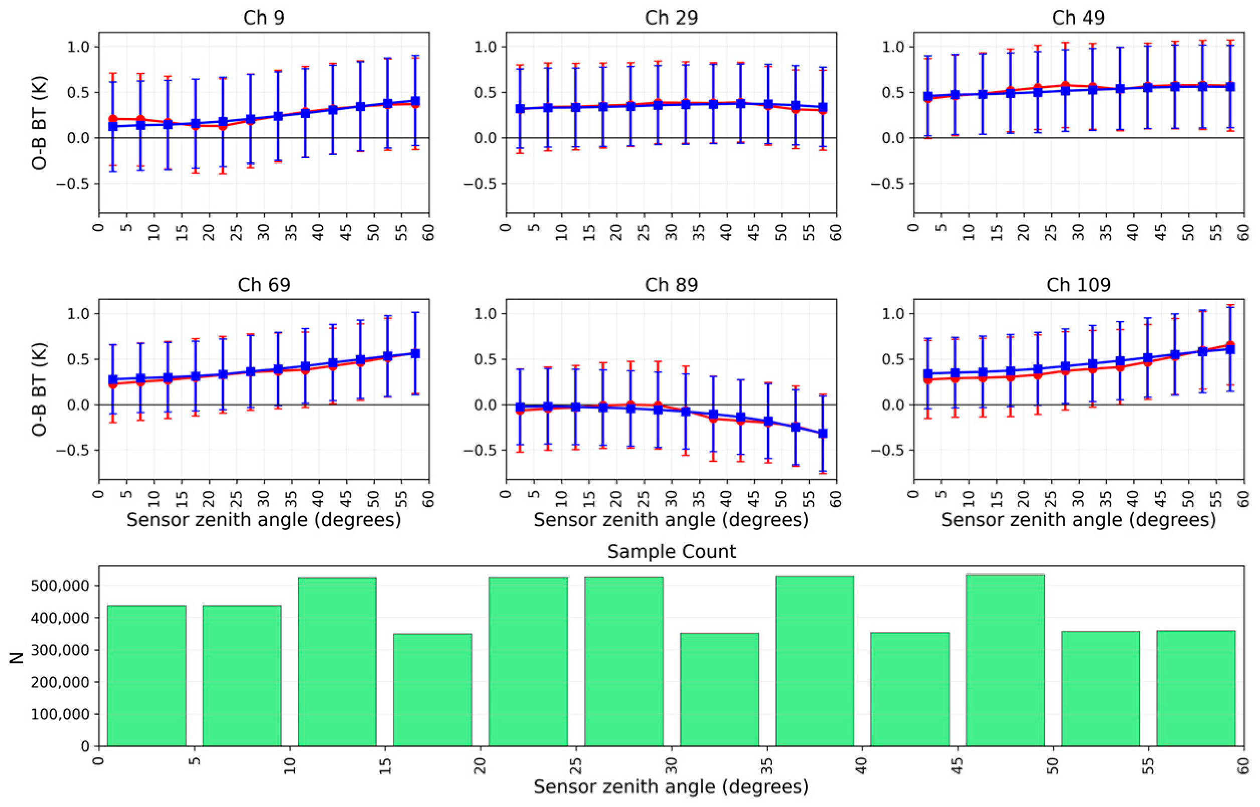
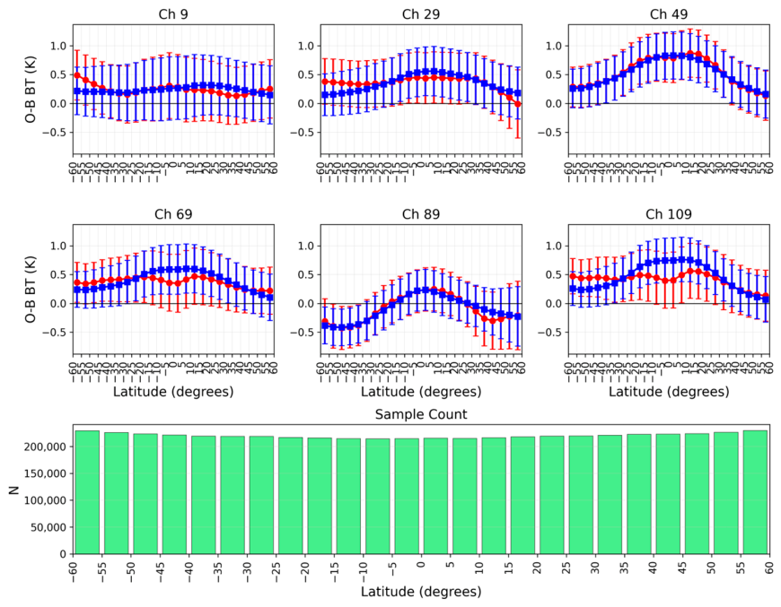
Additional evaluations were performed to examine the ability of CRTM-LNN to reproduce operational radiance diagnostics across different viewing geometries and atmospheric regimes, as shown in Figure 13 and Figure 14, respectively. The sensor-zenith-angle comparison shows substantially better consistency between IASI–AI and IASI–CRTM. Both reproduce nearly the same angular dependence: O–B increases with sensor zenith angle for Ch9, Ch69, and Ch109, remains relatively stable for Ch29, increases moderately for Ch49, and becomes increasingly negative for Ch89. Some channel-dependent offsets remain, but these differences are mostly modest and do not increase sharply toward the largest viewing angles. The similar trends and overlapping variability ranges indicate that CRTM-LNN does not introduce a strong additional scan-angle dependence relative to CRTM.

The latitude-binned comparison shows that IASI–AI and IASI–CRTM reproduce some common large-scale patterns, but their agreement is not uniformly close across latitude. Pronounced and spatially coherent differences occur in the tropics and Southern Hemisphere mid-to-high latitudes. For Ch9 and Ch29, IASI–AI is approximately 0.2–0.35 K higher than IASI–CRTM over the southern mid-to-high latitudes, indicating that the AI-predicted BTs are systematically lower than the CRTM simulations in this region. In contrast, Ch69 and especially Ch109 show substantially lower IASI–AI values over the tropics, with differences reaching roughly 0.20–0.4 K, indicating that the AI predicts warmer BTs than CRTM there. Ch89 shows its largest separation over the northern mid-to-high latitudes. Although the variability ranges often overlap, the persistence of these mean differences across several neighboring latitude bins indicates a structured latitude-dependent residual rather than random sampling noise. Thus, CRTM-LNN captures the broad geographical behavior but still shows important atmospheric-regime-dependent biases, particularly in tropical and southern mid-to-high-latitude conditions.

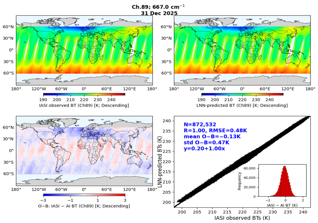
BT spatial comparisons were conducted across all six temporally independent evaluation days. Figure 15 presents the comparison for IASI Ch89 (667 cm⁻¹) on 31 December 2025 as an illustrative example. Ch89 was selected as a representative channel because it lies within the strongest CO₂ absorption region of the investigated 15 μm band. The emulator accurately reproduces the global BT distribution simulated by CRTM, including the large-scale latitudinal temperature gradients and regional atmospheric variability. The BT bias field shows only small, localized differences, with most regions remaining within ±0.5 K and no obvious large-scale systematic bias patterns. The scatterplot further demonstrates the excellent agreement between emulator predictions and CRTM simulations, yielding a correlation coefficient of 1.00, an RMSE of only 0.48 K, and a mean bias of −0.13 K. The bias histogram is nearly symmetric about zero, indicating negligible systematic error. Although only one representative channel and day are shown here, similar results were obtained for the remaining channels and independent evaluation days, demonstrating the emulator’s strong radiometric accuracy and generalization capability.

3.4. Evaluation of Model Performance on Calculation Speed

Training was conducted on a single computational node equipped with two NVIDIA A2 GPUs and two Intel Xeon Gold 6338 processors operating at 2.00 GHz, providing 128 logical CPU threads. The node contained approximately 1.0 TiB of system memory and ran Red Hat Enterprise Linux 9.8. The software environment included Python 3.12.9, PyTorch 2.6.0+cu126, CUDA 12.6, cuDNN 9.5.1, and NCCL 2.21.5. The complete 120-epoch CRTM-LNN training run required approximately 19 h. Although this represents a one-time offline training cost, the trained emulator provides substantial computational savings during repeated forward and Jacobian calculations.

The CRTM simulator driver was compiled with GNU Fortran 11.5.0 (-O3 -ffast-math -funroll-loops) and linked with -fopenmp, whereas the inspected CRTM forward-module object used GNU Fortran 8.5.0 with debugging and runtime checks (-ggdb -fbounds-check -ffpe-trap=overflow,zero,invalid) and no recorded -O3 or -fopenmp. Binary inspection suggests single-threaded CRTM execution despite 128 available logical threads. Reported speedups therefore apply to this specific build, rather than an optimized, multithreaded CRTM configuration.

The CRTM-LNN Jacobian calculations are parallelized across atmospheric profiles using one independent process per GPU. Dates are processed sequentially, but profiles within each date are divided into non-overlapping subsets and processed concurrently by the GPUs, each using its own copy of the trained model.

We have found that CRTM-LNN substantially accelerates the radiative-transfer calculations under the tested configurations. The reported CRTM-LNN wall-clock times include only the forward/Jacobian computations. For one day of data covering the 111-channel IASI CO₂ band, the CPU-based CRTM-LNN reduced the forward-simulation time from approximately 90 to 7.5 min relative to the CPU-based CRTM, corresponding to an approximately 12× CPU-to-CPU speedup. When executed on a single GPU, the emulator achieved an approximately 18× wall-clock speedup relative to the CPU-based CRTM. The differentiable tensor-based implementation also supports GPU parallelization for Jacobian generation, achieving approximately 2.5× and 5× system-level speedups using one and two GPUs, respectively, relative to the CPU-based CRTM tangent-linear calculation. Because the GPU and CRTM benchmarks use different hardware, these Jacobian speedups represent practical acceleration under the tested configurations rather than hardware-normalized algorithmic comparisons. Nevertheless, the combination of forward accuracy, explicit radiative-transfer consistency, and efficient batched forward and sensitivity calculations supports the potential use of CRTM-LNN in large-scale hyperspectral simulations, Jacobian generation, retrievals, data-assimilation research, and near-real-time remote-sensing applications.

Table 9. Computational configuration and timing summary.

Environment Item	Configuration
Active trainable parameter	45,616
Approximate FP32 parameter storage	0.18 MB
Compute nodes	1
GPUs	2 NVIDIA A2 GPUs
CPUs	2 Intel Xeon Gold 6338 processors at 2.00 GHz
Logical CPU threads	128
System memory	Approximately 1.0 TiB
Operating system	Red Hat Enterprise Linux 9.8
Python	3.12.9
PyTorch	2.6.0+cu126
CUDA runtime	12.6
cuDNN	9.5.1
NCCL	2.21.5
Distributed configuration	PyTorch DistributedDataParallel, two DDP processes, one per GPU
Per-GPU batch size	2048
Effective global batch size	4096
Training duration	~19 h
Forward timing	CRTM: ~90 min; CRTM-LNN: ~7.5 min on one CPU and ~5 min on one GPU
Averaged forward timing per profile per channel	CRTM: ~5.58 × 10−5 s; CRTM-LNN: ~4.65 × 10−6 s on one CPU and ~3.10 × 10−6 s on one GPU
Forward acceleration	Approximately 12×, CPU-to-CPU; 18×, CPU-to-one-GPU
Jacobian timing	CRTM tangent-linear: ~95 min on one CPU; CRTM-LNN: ~38 min on one GPU; ~19 min on two GPUs
Averaged Jacobian timing per profile per channel	CRTM tangent-linear: ~5.89 × 10−5 s on one CPU; CRTM-LNN: ~2.35 × 10−5 s on one GPU; ~1.18 × 10−5 s on two GPUs
Jacobian acceleration	Approximately 2.5×~5×, system-level
Peak forward runtime memory	0.2412 GB
Peak Jacobian runtime memory	0.1447 GB

summarizes the computational configuration and timing summary.

4. Discussion

4.1. Advantages, Computational Trade-Offs, and Current Scope of the Physics-Informed CRTM-LNN

The results of this study highlight several practical advantages of the integrated CRTM-LNN framework for radiative-transfer emulation. First, its ODE-inspired layer-wise state evolution is well aligned with the ordered and cumulative character of atmospheric radiative transfer. The LNN-LOD propagates a latent state through successive pressure layers while allowing the effective update to depend on the local thermodynamic and compositional conditions and the vertical context carried from preceding layers. Consequently, nearly transparent, weakly absorbing, and strongly absorbing layers can produce different hidden-state trajectories and update magnitudes. This behavior should be understood as input-conditioned state evolution: the model parameters remain fixed after training, while the hidden-state trajectory and gate values vary with each atmospheric profile. Although the hidden state is a learned latent representation rather than a physical radiance or optical-depth variable, this formulation provides a physically motivated and flexible mechanism for representing layer-to-layer dependencies across the atmospheric column.

Second, the interpretability and diagnostic capability of CRTM-LNN arise primarily from its explicit prediction of layer optical-depth increments and their propagation through the analytic radiative-transfer pathway,

$$\left(\mathit{X},\mathit{g}\right)\to ∆{\tau }_{\upsilon ,k}\to {\tau }_{\upsilon ,k}\to I_{\upsilon ,TOA}\to BT$$

This formulation makes layer and cumulative optical depth, transmittance, weighting or contribution functions, radiance, and brightness temperature directly available for evaluation. Model errors can therefore be diagnosed at multiple stages of radiance formation rather than solely through final BT agreement. Because the entire pathway is differentiable, atmospheric-state Jacobians can be generated through automatic differentiation of both the learned atmospheric-state-to-optical-depth relationship and the analytic optical-depth-to-radiance calculation.

Third, the configuration evaluated in this study provides a compact representation of vertical radiative-transfer behavior. The model contains 45,616 trainable parameters, compared with approximately 3.06 million parameters in the CRTM-MLP baseline. This comparison demonstrates the lower parameter and model-memory requirements of CRTM-LNN but should not be interpreted as the direct cause of its computational acceleration, which also depends on the computational graph, batching strategy, hardware, numerical precision, and implementation. In the forward-model benchmark, both CRTM and CRTM-LNN were executed on CPUs, and CRTM-LNN reduced the wall-clock time by approximately 12×, providing a relatively hardware-comparable measure of forward computational efficiency. For Jacobian generation, CRTM-LNN automatic differentiation using two GPUs was approximately 5× faster than the CPU-based CRTM tangent-linear calculation. Because the Jacobian benchmark involves different hardware platforms, this value represents the practical end-to-end acceleration obtained under the tested configurations rather than a hardware-normalized comparison of algorithmic efficiency.

The reported CRTM–LNN and CRTM–MLP results are based on a single training realization for each model. The standard deviations in Table 6, Table 7 and Table 8 characterize profile-to-profile variability within the evaluation dataset and do not quantify run-to-run training variability. Accordingly, the comparisons describe the evaluated model realizations, and the robustness of smaller performance differences across independent training runs remains unassessed.

A computational trade-off of the current CRTM-LNN architecture is that its layer-by-layer recurrence and two-stage state update introduce sequential operations along the 91-layer vertical grid, limiting vertical parallelism and increasing training and inference costs relative to fully feed-forward architectures, despite the model’s small parameter count. Nevertheless, once trained, its tensor-based GPU implementation supports efficient batched forward and Jacobian calculations over large numbers of atmospheric profiles and channels. These computational gains are particularly relevant to applications requiring repeated radiance and sensitivity evaluations, including large-volume observation-minus-background monitoring, rapid quality control, iterative atmospheric retrievals, channel-selection and information-content analyses, ensemble sensitivity experiments, and variational or ensemble-based data assimilation. In such applications, the accumulated cost of repeated CRTM calculations can become substantial. However, these speedup values apply only to the forward-model and Jacobian calculations tested in this study; the overall acceleration of an operational system will also depend on data input/output, preprocessing, quality control, minimization, and interprocess communication.

The current auxiliary-input branch includes sensor zenith angle, scan angle, sensor azimuth, surface pressure, and surface skin temperature. Not all these variables have an independent physical role in determining vertical atmospheric optical depth under the clear-sky, plane-parallel assumptions adopted here. In particular, sensor azimuth has no direct scalar radiative effect, surface skin temperature primarily controls the surface-boundary contribution, and sensor zenith and scan angles contain substantial geometric redundancy. Although direct supervision of layer optical depth and the independent viewing-angle evaluations limit evidence of substantial spurious behavior within the tested domain, the present structure does not strictly prevent the learned optical-depth predictor from exploiting sampling-related correlations. Future work will therefore compare reduced-input configurations, separate surface-boundary variables from the atmospheric optical-depth branch and test the invariance of predicted vertical optical depth under controlled changes in viewing geometry.

Applications involving window and surface-sensitive channels require a more complete treatment of the surface-boundary condition. Although channel-dependent surface emissivity can be introduced through the analytic solver, a realistic implementation must also account for surface skin temperature, reflected downwelling atmospheric radiance, spectral and angular emissivity variations, and differences among ocean, land, snow, and ice surfaces. These extensions are more direct than all-sky development because they modify the surface boundary rather than the atmospheric propagation equation, but they still require dedicated validation.

Extension to clouds, aerosols, and precipitation represents a substantially more difficult problem. Multiple scattering introduces angular coupling among radiances, interactions between upward- and downward-propagating radiation, and dependence on additional optical and microphysical properties, including scattering optical depth, single-scattering albedo, phase-function information, particle size, and cloud overlap. The current absorption-oriented, single-path hidden-state formulation may therefore require substantial modification, together with coupling to a differentiable multi-stream or multiple-scattering solver. Similarly, robustness under atmospheric regimes outside the training distribution must be established using independent datasets and controlled perturbation experiments rather than inferred solely from the input-conditioned LNN dynamics.

Overall, the principal strength of CRTM-LNN lies in the integration of ODE-inspired vertical state evolution, supervised layer-optical-depth prediction, and an explicit differentiable radiative-transfer pathway. This design provides physically interpretable intermediate quantities, supports automatic-differentiation-based Jacobian generation, and achieves substantial computational acceleration within the clear-sky spectral domain evaluated here. The identified trade-offs and current scope define the technical priorities for extending the framework to broader spectral, surface, and atmospheric applications.

4.2. Potential NWP Applications

CRTM-LNN has potential as a differentiable surrogate observation operator for future numerical weather prediction applications. CRTM is widely used for radiance simulation, observation-minus-background monitoring, quality control, atmospheric retrievals, and data assimilation. In these applications, the computational burden arises not only from individual forward simulations but also from repeated evaluations over large numbers of atmospheric profiles, spectral channels, retrieval iterations, and ensemble members. The demonstrated forward-model acceleration therefore suggests immediate research applications in large-volume O–B monitoring, rapid observation-quality assessment, synthetic-observation generation, channel-selection studies, iterative retrievals, and ensemble sensitivity experiments.

A particularly important application is atmospheric-state Jacobian generation for variational retrieval and data-assimilation systems. Because CRTM-LNN retains a differentiable pathway from atmospheric state to layer optical depth and from optical depth to radiance, forward simulations and radiative sensitivities can be obtained from the same trained emulator without requiring a separate neural Jacobian model. The encouraging temperature-Jacobian results indicate that this approach could reduce the computational cost of research-oriented retrieval and assimilation experiments while preserving vertically resolved sensitivity information. Before operational implementation, the Jacobians should be evaluated more broadly across channels, atmospheric and surface variables, viewing geometries, and geophysical regimes. Their effects on retrieval convergence, analysis increments, and forecast performance should also be tested within actual assimilation systems.

The explicitly retained intermediate radiative quantities may provide additional value for observation monitoring and model diagnosis. Differences between CRTM-LNN and CRTM can be examined in layer optical depth, cumulative optical depth, transmittance, weighting function, radiance, and BT space. This allows a discrepancy to be traced more directly to the atmospheric optical-depth prediction, vertical radiative structure, surface-boundary condition, or final radiance calculation. Such diagnostics could support channel quality control, bias characterization, sensitivity analysis, and the development of emulator-specific model-error estimates for retrieval and assimilation applications.

The most immediate NWP applications are therefore clear-sky forward simulation, large-scale O–B monitoring, sensitivity analysis, and research-oriented retrieval and data-assimilation experiments. Progress toward operational use will require broader independent validation, characterization of emulator bias and uncertainty, testing of numerical stability and local linearity, evaluation within complete retrieval or assimilation workflows, and documentation of throughput and memory requirements under operational workloads. These system-level experiments will determine whether the computational and diagnostic advantages demonstrated here translate into measurable benefits in complete NWP applications.

5. Conclusions

A physics-informed CRTM-LNN AI Emulator for atmospheric hyperspectral radiative transfer is demonstrated using IASI observations within the 15 μm CO₂ absorption band in this study. The vertical evolution of optical depth is represented using a layer-by-layer optical-depth Liquid Neural Network with ODE-like dynamics. By coupling neural-network-predicted optical depths with an analytic radiative-transfer solver, the framework maintains physical interpretability and consistency while significantly reducing the computational complexity of hyperspectral radiative-transfer calculations. The CRTM–LNN emulates CRTM, which is itself a fast, parameterized radiative transfer model; therefore, the reported emulator–CRTM comparison metrics quantify agreement with CRTM rather than absolute radiometric accuracy, and accuracy relative to independent line-by-line calculations has not been assessed in this study.

The CRTM-LNN emulator closely reproduced CRTM brightness temperatures, with representative channels exhibiting small mean global, channel-mean biases (<0.1 K), along with small channel standard deviations typically below 0.2 K. Observation-minus-background analyses against IASI observations further showed that CRTM-LNN preserves the major channel-, latitude-, and sensor-zenith-angle-dependent characteristics of CRTM. Residual differences remain channel-dependent and are most pronounced in the tropics and Southern Hemisphere mid-to-high latitudes, whereas viewing-angle offsets are generally smaller and do not systematically increase at large zenith angles. These results demonstrate strong overall radiometric consistency while identifying specific atmospheric regimes and channels that could benefit from improved regime balancing and channel-aware optical-depth refinement.

Extensive evaluations were also performed on physically meaningful radiative-transfer diagnostics, including cumulative optical depth, atmospheric transmittance, weighting functions, and Jacobians. The emulator accurately reproduced the vertical structure and spectral variability of the layer-means of these quantities. The close agreement between the CRTM-LNN and CRTM demonstrates that the proposed framework not only predicts radiances accurately but also preserves the underlying radiative-transfer physics governing atmospheric absorption, transmission, and vertical radiative sensitivity. The consistency between the aggregated and daily statistics further indicates stable and robust model performance across a wide range of atmospheric conditions.

Automatic-differentiation-based analyses demonstrate that CRTM-LNN reproduces the magnitude and vertical structure of CRTM temperature Jacobians while supporting efficient GPU-accelerated sensitivity calculations. Relative to the CRTM-MLP baseline, CRTM-LNN achieves lower RMSE, higher correlations, reduced profile-to-profile variability above 1 hPa, and substantially smoother vertical structures below 200 hPa, although improvements in peak-pressure location remain channel-dependent. CRTM–LNN reduces absolute centroid-pressure errors across all evaluated channels, yielding errors of 1.77–5.01 hPa compared with 5.88–8.17 hPa for CRTM–MLP. These results indicate improved vertical localization of temperature Jacobian sensitivities, although the magnitude of improvement varies by channel. For CO₂, CRTM-LNN markedly reduces RMSE and roughness mismatch and generally improves correlation; however, the remaining low correlations and inconsistent peak- and centroid-pressure improvements indicate that accurate CO₂ Jacobians remain challenging. This limitation likely reflects the weak CO₂ radiative sensitivity and the restricted CO₂ variability imposed by the cap in the current CRTM configuration. Overall, these findings demonstrate the value of preserving the explicit layer-optical-depth-to-BT pathway for representing the local differential structure of radiative transfer, particularly for temperature sensitivities, while motivating future improvements through broader CO₂ variability and targeted sensitivity constraints. The MLP comparison provides supporting context rather than a universal ranking of neural architectures, and the results support further evaluation of CRTM-LNN as a differentiable surrogate observation operator for atmospheric retrieval and data-assimilation applications.

The present findings should be interpreted within the defined scope of this study. The current evaluation considers 111 IASI channels in the 15 μm CO₂ absorption band under clear-sky, absorption-only conditions and uses the fixed ECMWF91L vertical grid. Detailed atmospheric-state sensitivity evaluation is focused primarily on temperature Jacobians, while weaker sensitivities to water vapor, ozone, and CO₂ require further quantitative assessment. The results do not establish that the same accuracy, computational efficiency, or Jacobian coherence will necessarily persist under cloudy or scattering conditions. Extending the framework to the full IASI spectrum—including surface-sensitive and window channels—and to cloudy, aerosol-laden, and precipitating conditions would present substantial additional challenges. Full-spectrum implementation would greatly increase the output dimensionality and require a realistic treatment of surface emissivity; maintaining computational efficiency may therefore require channel embeddings, parameter sharing, low-rank spectral representations, or principal-component compression. All-sky applications would additionally require explicit representation of scattering optical properties and coupling to a differentiable multi-stream or multiple-scattering radiative-transfer solver.

Overall, our study demonstrates that the proposed physics-informed CRTM-LNN AI Emulator provides an efficient and physically interpretable potential alternative to conventional radiative-transfer calculations while maintaining high radiometric accuracy and radiative-transfer consistency. The proposed framework offers a promising pathway toward next-generation AI-enabled radiative-transfer modeling for hyperspectral infrared observations.