Unified Multi-Application Segmentation of High-Resolution Satellite Images Through Consensus-Based Probabilistic Fusion

Highlights

What are the main findings?

• Probability Fusion via Multiple Model Instances: Achieved pixel-wise class probability estimation by leveraging the collective intelligence of per-dataset model instances trained on heterogeneous remote sensing datasets.
• Improved Cross-Dataset Performance: Demonstrated enhanced generalization capabilities across various segmentation architectures while maintaining original intra-dataset accuracy.

What are the implications of the main findings?

• Customizable Unified Label Configuration: Allows users to flexibly scale or tailor a single unified label space to meet specific target application needs.
• Improved Generalization without Additional Annotation: Provides reliable generalization to unseen aerial imagery without requiring the labor-intensive production of huge, human-labeled target datasets.

Abstract

Deep-learning-based land cover segmentation models for high-resolution aerial images often suffer from inconsistent performance on unseen data due to limited spatial and temporal dataset ranges alongside inherent labeling inconsistencies. Existing solutions, such as foundation models and unsupervised domain adaptation, offer indirect improvements but require considerable post-processing or transfer learning. To address this limitation, this study introduces a direct dataset integration method that fuses heterogeneous datasets with disparate class compositions into a single operational framework. For each individual dataset, multiple model instances (MMIs) predict pixel-wise class probabilities. These probabilities are subsequently combined within a single, unified, and customizable label space, enabling improved generalization to unseen domains without additional manual annotation. We applied and validated this method using three benchmark remote sensing datasets: OpenEarthMap, FLAIR, and the cloud dataset based on high-resolution optical satellite imagery (KOMPSAT-3 and 3A), sourced from the official AI-Hub platform in South Korea. Across both 2-fold and holdout tests, statistical validation confirmed that the unified model enhances generalization on untrained imagery (p < 0.0001) while reliably maintaining or slightly improving original intra-dataset accuracy. Furthermore, it successfully consolidates diverse land-cover categories with atmospheric features such as clouds, which were previously handled only by separate dedicated models.

1. Introduction

AI-based pixel-level classification, also widely conceptualized as semantic segmentation, has emerged as a cornerstone methodology for automated land cover mapping in high-resolution remote sensing imagery. By training deep convolutional neural networks (CNNs) or vision transformers on large-scale datasets, these advanced frameworks typically yield significantly more accurate, detailed, and contiguous segmentation results compared to classical pixel-based or object-based alternative methods [1,2,3]. Despite these remarkable technological advancements, a pervasive and fundamental limitation of complex machine learning classifiers remains their inherent tendency to overfit the specific statistical distributions of their training samples. While these highly parameterized deep learning models exhibit exceptional performance and near-perfect accuracy when evaluated within their native training datasets, they frequently manifest unexpectedly poor and degraded performance when deployed on unseen images captured outside their initial training environment [4,5,6].

This critical generalization bottleneck primarily arises from explicit and implicit limitations embedded within the remote sensing datasets themselves. High-resolution aerial and satellite images are highly sensitive to vast environmental and technical variations, including geographic locations, seasonal timings, multi-temporal atmospheric conditions, sensor degradation, and disparate imaging source specifications. Typically, a public or commercial dataset is meticulously curated for a specific object of interest or regional project, operating under a constrained geographic scope, tight project timeframes, and fixed institutional budgets. For instance, a dataset optimized for urban planning in European cities will feature distinct architectural topologies, solar angles, and spectral signatures that do not align with agricultural monitoring datasets in Asian regions. Consequently, a deep learning model highly optimized for one specific dataset often struggles to perform effectively when presented with imagery from an entirely different dataset, leading to severe domain shift issues that hinder practical, large-scale deployment.

To alleviate these domain shift challenges and improve the overall generalization capabilities of deep learning architectures in remote sensing land cover mapping, three distinct methodological paradigms have been extensively studied by the geospatial community, each offering unique technological strengths alongside distinct operational and architectural limitations.

First, Unsupervised Domain Adaptation (UDA) frameworks have gained significant traction and academic visibility due to their theoretical ability to address severe domain shifts without requiring labor-intensive ground-truth annotations in the newly encountered target domain, as exemplified by domain-adaptive benchmarks like LoveDA [7]. By utilizing adversarial training strategies, maximum mean discrepancy (MMD) alignments, or category-certainty attention formulations, UDA source-to-target alignment provides a cost-effective operational strategy for cross-regional model deployment [8]. However, traditional UDA paradigms are inherently unidirectional and local, as they focus exclusively on optimizing the distribution shift for a single, predefined target domain. This localized distribution alignment tends to force the network’s latent space to overfit that specific target domain, thereby compromising the model’s capacity to generalize universally when subsequently exposed to entirely unseen geographical regions or alternative sensor modalities.

Second, Geospatial Foundation Models have recently transformed the remote sensing paradigm by providing highly robust, generalizable, and self-supervised feature representations that are pre-trained on massive, uncurated image datasets covering continental scales via advanced continual pre-training [9] and multitemporal configurations like Prithvi-EO-2.0 [10]. Leveraging masked autoencoders (MAE) or specialized frameworks tailored for multi-spectral and temporal satellite dynamics like SatMAE [11], these massive foundation models excel at capturing intricate spatial contexts, texturing patterns, and geometric structures that standard supervised architectures often completely overlook. They inherently internalize critical confounding factors within their deep foundational weight layers. However, it is vital to recognize that a geospatial foundation model operates predominantly as an indirect teacher or a highly capable starting backbone rather than a plug-and-play semantic solution. To translate these self-supervised representations into accurate, pixel-wise semantic labels, a subsequent fine-tuning or transfer learning stage remains mandatory. This downstream adaptation process inevitably reintroduces the strict requirement for explicitly labeled target datasets.

Third, manually fused benchmarks, with the OpenEarthMap dataset serving as a prominent pioneering example for global high-resolution mapping [12], offer highly reliable, expert-curated ground-truth templates that successfully capture the real-world diversity of global geography and distinct imaging sensors. By collecting and organizing disparate datasets into a unified framework, these benchmarks create a robust, standardized baseline for rigorous multi-regional validation, expanding the scope of fine-grained recognition over complex terrains [13]. These combined resources accurately reflect the true, intrinsic categorical variations found across complex global terrains and heterogeneous land-use types. However, this manual harmonization approach is heavily constrained by the extreme structural rigidity of its static taxonomy. Because these benchmarks rely on strictly predefined, hard-coded structural rules to align different label configurations, introducing a modified, fine-grained class type demands ongoing, labor-intensive human annotations and re-labeling efforts, which severely hinders the framework’s ability to scale dynamically in production.

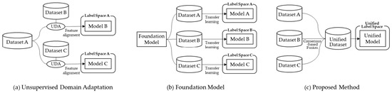
To systematically overcome these multi-faceted limitations, this paper introduces a novel data-centric fusion strategy that directly harnesses the probabilistic agreement among multiple model instances (MMIs) generated from both intra-dataset and cross-dataset perspectives. To illustrate the operational bottlenecks of existing methodologies and how they are resolved by the proposed method, Figure 1 compares the structural workflows of existing paradigms with our approach assuming a scenario with three heterogeneous datasets, each featuring distinct domain distributions and label taxonomies (Datasets A, B, and C).

Figure 1. Structural comparison of cross-dataset generalization paradigms across three heterogeneous datasets: (a) Unsupervised Domain Adaptation (UDA), which forces target domains into a rigid source taxonomy (Label Space A); (b) Geospatial Foundation Models, requiring separate fine-tuning that results in fragmented models (Label Spaces A, B, C); and (c) our proposed approach, which integrates disparate datasets into a single Unified Dataset with a customizable unified label space.

As shown in Figure 1a, UDA aligns feature distributions in a unidirectional manner toward a single source dataset. This limitation forces all resulting downstream models to be strictly tied to the source’s inherited taxonomy (Label Space A). Meanwhile, Geospatial Foundation Models, depicted in Figure 1b, provide powerful self-supervised feature representations. However, translating these features into operational models necessitates separate downstream fine-tuning stages, yielding fragmented models (Models A, B, and C), each confined to its native label space (Label Spaces A, B, and C).

In contrast, our approach (Figure 1c) operates entirely at the data level. By utilizing MMIs to reconcile label discrepancies before final model training, our framework consolidates disparate datasets into a single unified dataset to train a single model. This model can be deployed across a broad and customizable label space without incurring additional overhead from active ensembles or requiring architectural modifications during inference.

Our approach is fundamentally distinct from traditional model ensembles and standard probability fusion methods. While classic ensembles aim to reduce variance during inference using a static and uniform taxonomy, our proposed method emphasizes a data-centric pre-training phase that integrates diverse, heterogeneous taxonomies into a single, cohesive, and customizable label space. Moreover, unlike domain generalization and unsupervised domain adaptation (UDA) frameworks that rely on complex, localized alignments at the feature or representation level, our method shifts the harmonization process entirely to the label space.

The proposed methodology intentionally prioritizes structural universality over optimization for a single target domain, thereby ensuring robust and consistent generalization across diverse dataset distributions. Additionally, because alignment occurs in the label space rather than through intrusive modifications at the network level, our framework remains strictly model-agnostic. Consequently, it can be seamlessly applied to various state-of-the-art segmentation architectures without adding any computational overhead during inference.

To contextualize our methodology within the existing literature, Table 1 provides a systematic comparison of our proposed method against established paradigms, including traditional model ensembles, conventional probability fusion, and UDA. As shown in Table 1, traditional ensembles are computationally expensive during inference, and UDA frameworks are inherently constrained by a static taxonomy derived from the source domain. In contrast, our consensus-based probabilistic fusion framework creates a customizable and unified label space without requiring model modifications or introducing test-time computational penalties.

Table 1. Key operational and structural differences between the proposed method and existing training/inference paradigms.

Dimension	Traditional Model Ensembles & Probability Fusion	Domain Generalization/ Adaptation (UDA)	Proposed Method
Operational Phase	Inference phase (combining outputs during testing/deployment)	Training phase (aligning latent representations)	Data-centric pre-training phase
Target Label Space	Static, and identical (all models must share the exact same taxonomy)	Static taxonomy (strictly predefined by the source domain)	Unified & customizable
Mathematical Mechanism	Variance reduction (e.g., voting or averaging softmax probabilities)	Feature distribution alignment (using adversarial losses or MMD)	Pixel-wise joint class probability estimation & loss scaling
Inference Overhead	Very High (must run multiple model instances in parallel)	None (usually a single model is deployed)	None (only a single, unified model is deployed at inference)

Evaluating the architectural consistency, robustness, and applicability of this design, we conducted an extensive empirical analysis of the proposed framework across state-of-the-art network configurations. To ensure empirical validity, our evaluation encompasses diverse backbone networks utilizing multi-scale convolutional neural network (CNN) hierarchies—specifically including ResNet [14], ConvNeXt [15], and HRNet [16]—as well as global-context-aware Vision Transformers such as the Swin Transformer [17] and the Mix Transformer (MiT) within the SegFormer framework [18]. In addition, to thoroughly evaluate our framework under contemporary structural paradigms, we extend our benchmarking to modern SOTA milestones: ViT-CoMer [19], which features bidirectional multi-scale interaction between CNN and Transformer layers, and UniRepLKNet [20], which leverages large-kernel convolutions for expanded receptive fields. By incorporating these hybrid and large-kernel architectures, we demonstrate that our data-centric, label-space alignment mechanism achieves robust, architecture-agnostic cross-dataset generalization without being constrained by the underlying feature extraction mechanics.

Complementing these backbones, we extensively validated our framework across a wide range of established semantic segmentation decoders and heads. This includes traditional context aggregators like the PSPNet [21], DeepLabV3+ [22], and UperNet [23], advanced object-contextual representations (OCRNet) [24], and recent architectures driven by advanced attention or dynamic kernel formulations, including SegFormer [18], K-Net [25], and Mask2Former [26].

The practical effectiveness of the proposed framework was validated using three large-scale, heterogeneous remote sensing datasets featuring different class schemas: the OpenEarthMap dataset [12], the FLAIR dataset [27], and the cloud dataset from AI-Hub in South Korea [28]. Statistical evaluations across both 2-fold cross-validation and holdout testing protocols confirm that our unified model consistently enhances cross-dataset generalization performance while maintaining native intra-dataset accuracy. Notably, the framework consolidates diverse land-cover classes into a single, customizable label space. This unified schema achieves what was previously only possible through multiple separate, specialized models.

2. Materials

In this study, we used three publicly accessible datasets: OpenEarthMap, FLAIR, and the AI-Hub cloud dataset. All of the datasets are for semantic segmentation and have high-quality masks generated from aerial or satellite imagery. However, the configurations regarding image sources, spatial resolutions, class compositions, and strategies for collecting image locations are entirely different. Table 2 summarizes the detailed configurations of the datasets.

Table 2. Comparison of dataset configurations.

Dataset	OpenEarthMap	FLAIR	AI-Hub Cloud
Image source	From existing benchmarks (e.g., xBD, Inria, SpaceNet)	Aerial imagery (BD ORTHO) from IGN	Satellite imagery (KOMPSAT-3 and KOMPSAT-3A)
Spatial resolution	0.25 m–0.5 m	0.2 m	0.55 m–0.7 m
Spectral bands	R, G, B	R, G, B	R, G, B, NIR
Bit depth	8 bits	8 bits	16 bits
Target classes	Bareland, Rangeland, Developed space, Road, Tree, Water, Agricultural land, Building and Background	Building, Pervious surface, Impervious surface, Bare soil, Water, Coniferous, Deciduous, Brushwood, Vineyard, Herbaceous vegetation, Agricultural land, Plowed land, and Background	Thick cloud, Thin cloud, Cloud shadow, and Clear sky
Imaging locations	97 regions across 44 countries on 6 continents	50 to 74 departments in metropolitan France	Various global regions with different surface conditions

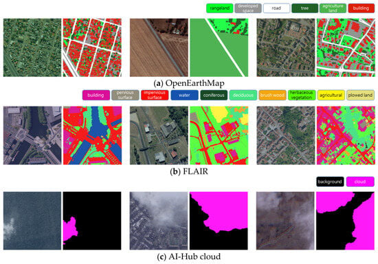
Figure 2 displays samples of images along with their corresponding labels from each dataset. For the cloud dataset, we combined the thin and thick cloud classes into a single cloud class while considering both the shadow and clear-sky classes as the background class.

Figure 2. Samples of image-label pairs from datasets.

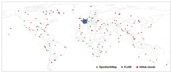
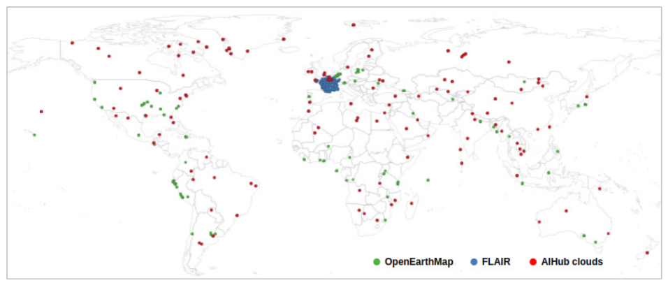
Figure 3 illustrates the image locations of each dataset. OpenEarthMap and the cloud dataset have a global scope for universal model training, while FLAIR focuses region-specific land cover characteristics of France.

Figure 3. Spatial locations of training images for each dataset.

2.1. Image Processing

We standardized the spatial resolution of images from the datasets, which ranged from 0.25 m to 0.7 m, to 1.0 m in order to create a single model suitable for various satellite imagery. The cloud dataset images were transformed from 16-bit to 8-bit using 1% percentile stretching for each band, and the NIR channel was removed for data uniformity.

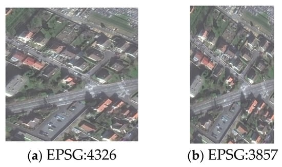
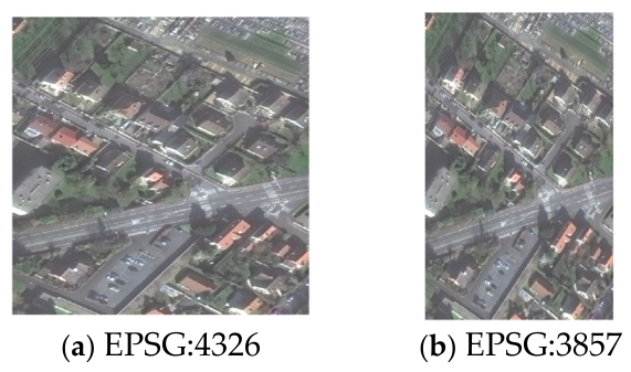
Some images from OpenEarthMap utilize the EPSG:4326 coordinate system, where geographic coordinates are expressed in degrees. Depending on the latitude of an image, the aspect ratio may differ from 1.0 in meters [29]. In such cases, the aspect ratio is adjusted to 1.0 after converting to EPSG:3857, ensuring that objects appear independent of latitude. Figure 4 displays “paris_3.tif” from OpenEarthMap in both EPSG:4326 and EPSG:3857 formats. The aspect ratio in EPSG:4326 is significantly distorted because the actual distances of the longitudinal and lateral dimensions differ by more than 1.5 times. This indicates that coordinate conversion and aspect ratio adjustment are essential steps for both training and inference.

Figure 4. Difference in the appearance of “paris_3.tif” according to the coordinate system.

2.2. Patchification and Sample Augmentation

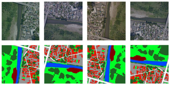
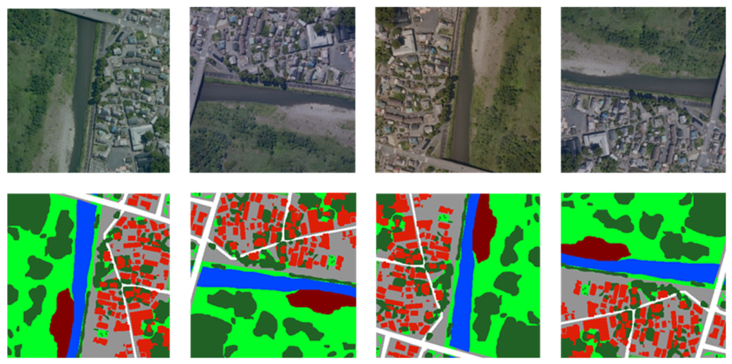
The input layer’s patch size is set to 320 × 320 pixels (320 m × 320 m) to ensure the visibility of target classes alongside relevant background. Each patch is extracted with a half-size overlap. During data extraction, a random multiple of 90-degree rotations is applied to enforce geometric invariance against varied satellite orbit trajectories, building upon established survey paradigms in image segmentation [30]. Furthermore, to simulate diverse environmental and atmospheric variations common in heterogeneous remote sensing imagery, color modification is implemented by injecting Gaussian noise N(0.0, 5.0) into both the C_b and C_r channels within the YC_bC_r color space. Compared to conventional RGB-space perturbations, augmenting data within these decoupled luminance-chrominance channels has been proven to enhance structural robustness under fluctuating solar illumination and radiometric discrepancies, thereby effectively stabilizing dense, pixel-wise prediction tasks under challenging, real-world satellite observations [31,32]. Figure 5 shows an example of the sample augmentation. The process retains the brightness and contrast while only changing the color information.

Figure 5. An example of data augmentation through patchification, where the upper panels display the augmented images and the lower panels show the corresponding ground-truth (GT) masks.

3. Methods

3.1. Proposed Process for Unifying Heterogeneous Datasets

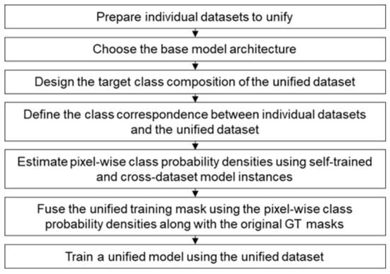
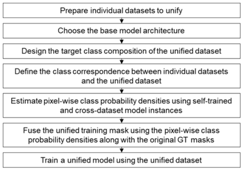
Figure 6 illustrates the overall process of the proposed method. In this study, we utilize three datasets to demonstrate the method’s effectiveness. While the mathematical formulation naturally extends to additional datasets through modular taxonomy expansion and incremental MMI cross-inference, practical scaling across larger multi-dataset collections involves specific label-harmonization trade-offs (discussed in Section 5).

Figure 6. The overall process of training a unified model by combining heterogeneous datasets.

The first step involves preparing the datasets for unification. In real-world scenarios, many datasets are created for various purposes. Often, individual datasets lack the variability of the source images. By combining these datasets, we can enhance variability, but due to different configurations, simple concatenation is not feasible. For this step, we selected three datasets as outlined in the Section 2: OpenEarthMap, FLAIR, and the AI-Hub cloud dataset.

The second step involves selecting a base model architecture to analyze the datasets. The sole purpose of this step is to generate a unified dataset, which will then serve as the foundation for training unified models across various architectural configurations. Various network architectures were evaluated using the MMSegmentation (v1.2.2) framework built on PyTorch (v2.10.0). To seamlessly integrate and test the latest backbone models, including ViT-CoMer and UniRepLKNet, the open-source mmseg-extension library was utilized (version commit 6a3996a, available online: https://github.com/chenller/mmseg-extension, accessed on 7 September 2026).

The third step outlines the composition of classes within the unified dataset. The design of the unified label space is fully customizable to meet specific application requirements, ranging from the full superset of all datasets to any of its subsets, provided that the correspondence between individual classes and the unified classes is clearly defined. In this study, we utilize the full superset to facilitate a quantitative performance comparison between dedicated models and the unified model trained within this unified label space. For a direct 1:1 comparison, a proper inverse-mapping mechanism from the unified label space back to each individual label space must be established (see Section 3.3).

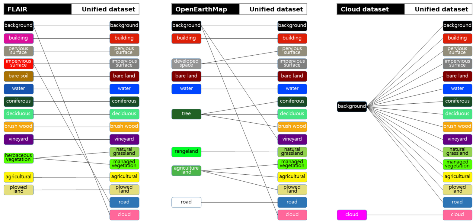
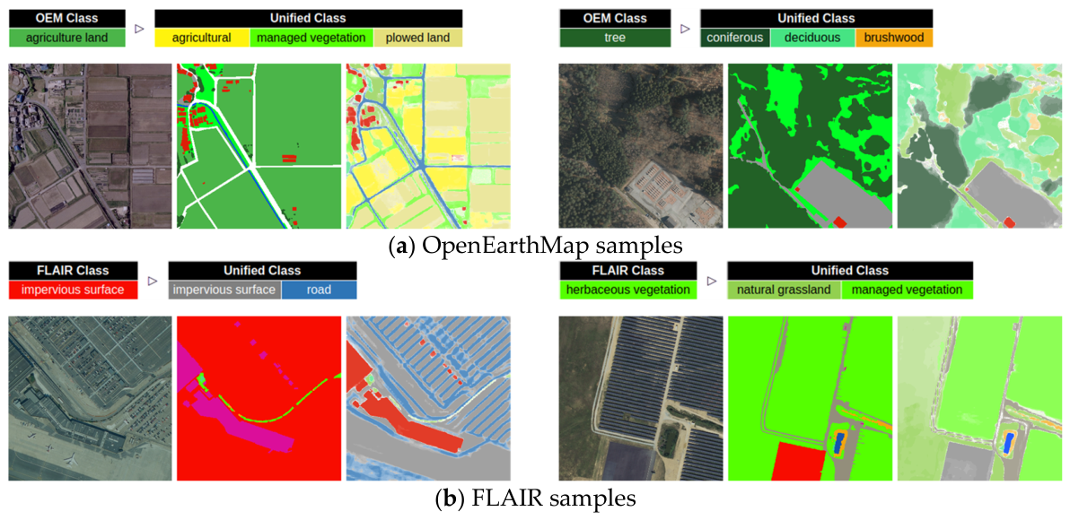
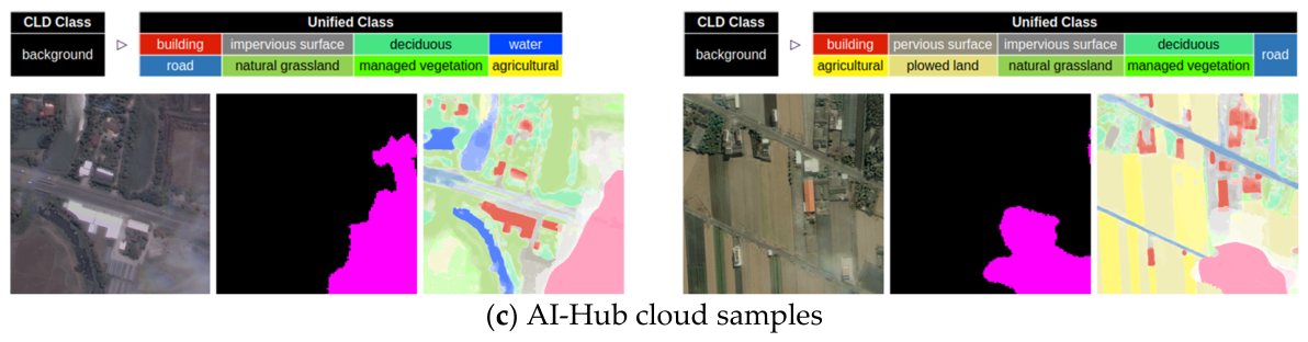
The FLAIR label space includes almost all classes except for the road and cloud classes. Even after adding these two classes, semantic ambiguity remained with the herbaceous vegetation class. In our initial design, we did not subdivide this class, which consequently led to high confusion among class instances. After examining the characteristics of herbaceous vegetation in the FLAIR dataset, we split it into natural and managed categories, ensuring a clear mapping to the OpenEarthMap label space. This adjustment resolved much of the confusion and allowed us to finalize the design. Figure 7 illustrates the relationship between the classes of each individual dataset and those of the unified dataset.

Figure 7. The correspondence between individual and the unified dataset classes.

The tree and agricultural land classes in OpenEarthMap are subdivided into more specific categories. The cloud class remains entirely unknown for both OpenEarthMap and FLAIR, while all classes other than the cloud class are considered unknown for the cloud dataset. These unidentified classes are mapped to their corresponding background classes.

The next step involves training MMIs for each dataset. Each instance utilizes a different combination of training and validation sets to yield distinct inference results. These results are then combined to generate pixel-wise class probabilities, denoted as P(k) for a class index k, which reflect the consensus within the dataset [33]. A sample is used for the validation by certain models. The number of these instances is calculated by multiplying the number of total instances by the validation data ratio, which in turn determines the number of levels of P(k).

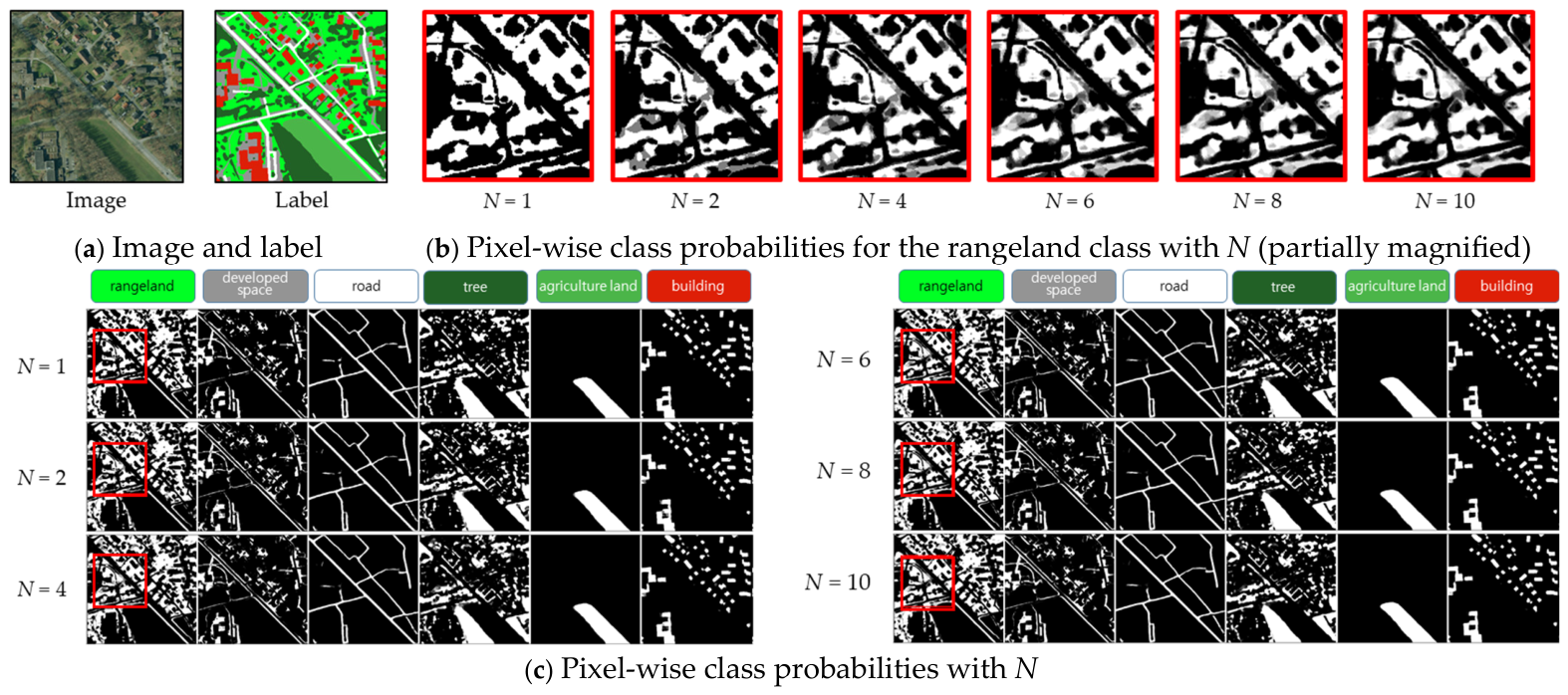
Figure 8 shows an OpenEarthMap example, displaying the original image, ground truth labels, and pixel-wise class probabilities as a function of the number of MMIs. As the number of MMIs (N) increases, the probability resolution improves by a factor of N. We observed that aggregating six MMIs yields sufficient probability information. Furthermore, we set the validation rate for each instance to 0.3—larger than the standard 0.2—because the MMIs collectively can achieve 100% coverage of the training data. Since the probability estimation for a given sample must be conducted by MMIs that did not use it during training, a total of 20 MMIs are required to guarantee at least 6 MMIs for estimation under this validation ratio, thereby resulting in six discrete levels for P(k).

Figure 8. Comparison of pixel-wise class probabilities with respect to the number of estimating MMIs (N). (a) The target image and the associated GT label; (b) partially magnified pixel-wise class probabilities for the rangeland class; and (c) the full pixel-wise class probabilities with N. The regions indicated by red rectangles in (c) are magnified in (b).

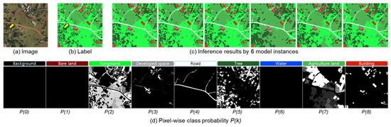
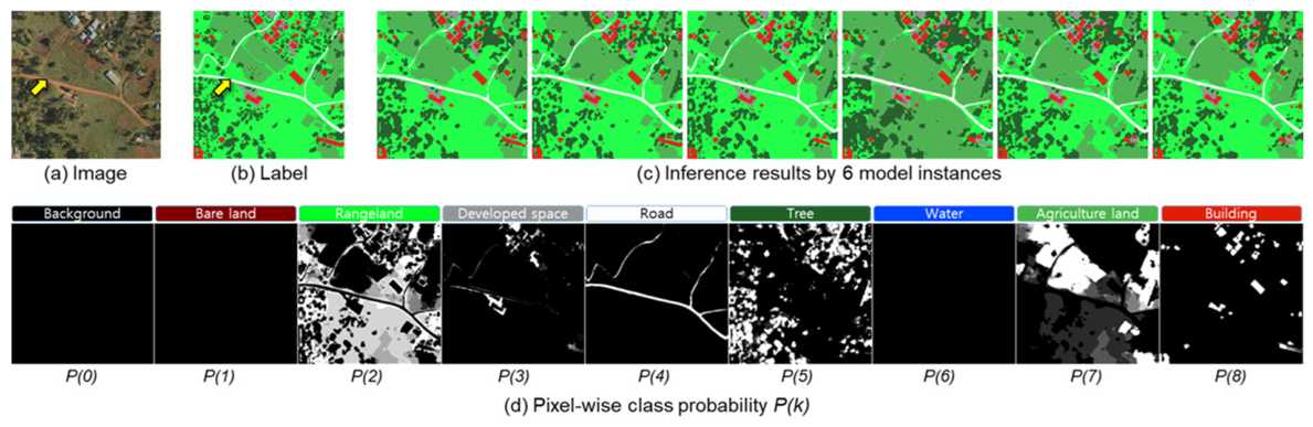
Figure 9 shows an OpenEarthMap example of MMIs forming a pixel-wise class probability. The yellow arrow in the image indicates the position that the majority of instances consider to be agricultural land, despite the GT class being rangeland.

Figure 9. An OpenEarthMap example of model instances forming a pixel-wise class probability. In the area indicated by the yellow arrow, model instances tend to expect the region to be agricultural land while the label is rangeland.

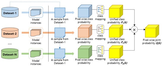
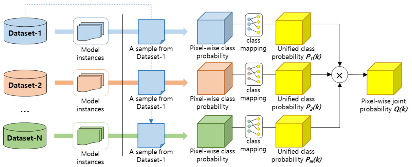
Pixel-wise class probabilities can also be generated by using cross-dataset MMIs, providing another perspective on the ensemble-based consensus across different datasets. Ultimately, the probabilities at each pixel location are multiplied—similar to the approach of the Naive Bayes classifier—and then normalized to sum to 1.0, yielding a pixel-wise joint probability [34]. Figure 10 outlines the steps for data processing, while Figure 11 provides an example of fusing the pixel-wise joint probability.

Figure 10. Calculation of pixel-wise joint probability using self-trained model instances and cross-dataset model instances.

Figure 11. An example of computing the pixel-wise joint probability for an OpenEarthMap patch by fusing pixel-wise class probabilities, each generated by per-dataset model instances.

There is an important consideration to keep in mind. When working with two datasets, A and B, classes that appear only in dataset B may be classified as part of the background class in dataset A. When calculating the joint probability of a pixel belonging to such a class in dataset B, it is reasonable to reduce the weight of the probability estimates derived from MMIs trained on dataset A. For example, the cloud class is never seen by models trained on OpenEarthMap. When computing the joint probability of pixels where the GT is the cloud class, the probability derived from OpenEarthMap MMIs is assigned a lower weight.

A pixel-wise joint probability for class k is calculated with the weights as follows:

$$Q\left(\mathrm{k}\right)={\left\{ {\displaystyle {\displaystyle \prod }_{i=1}^N}{P}_i{\left(k\right)}^{w_i\left(k\right)} \right\}}^{ {\displaystyle \frac{1}{{{\displaystyle \sum }}_i{w}_i\left(k\right)}}} ,$$

(1)

where $P_i\left(k\right)$ represents the pixel-wise class probability for class k estimated by MMIs trained on dataset i, and $w_i\left(k\right)$ is the corresponding weight. Normally, the weights are set to 1.0; however, if a class is unique to a specific dataset, a lowered weight—referred to as the ignorance factor—is applied to probabilities derived from irrelevant datasets.

The final step to unify datasets involves harmonizing the individual masks based on pixel-wise joint probabilities. Each pixel location is assigned a consensus class label with an associated confidence level, functioning as a loss weight to train the unified model. We refer to the class with the highest probability as the dominant class; its class index is denoted as $c_D$, and its joint probability is represented by $Q\left(c_D\right)$. The set G represents the class indices in the unified label space, corresponding to a GT class of the individual dataset, and the sum of their probabilities is referred to as $P_G$ as in

$$P_G={\displaystyle \sum }_{k\in G}Q\left(k\right) .$$

(2)

Considering these factors, we can identify three specific cases. If the $c_D$ is part of set G, it is clear that the resulting class index becomes $c_D$, with a confidence level of $Q\left(c_D\right)$. If $c_D$ is not in set G and $Q\left(c_D\right)$ exceeds $P_G$, it indicates that the dominant class is overwhelming the original GT class. In this case, the target class index is assigned to $c_D$, while its confidence $Q\left(c_D\right)$ is adjusted by subtracting $P_G$. If $Q\left(c_D\right)$ is smaller than $P_G$, it indicates that the outcome of the majority vote has minimal impact on the pixel. In this scenario, the original GT class remains unchanged. However, within the unified label space, an individual GT class can be subdivided into multiple classes. As a result, the class ($c_G$) with the highest confidence score within G is used to represent the group. The associated confidence score, $Q\left(c_G\right)$, is then reduced by the ratio of 1.0 − $Q\left(c_D\right)/P_G$.

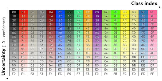
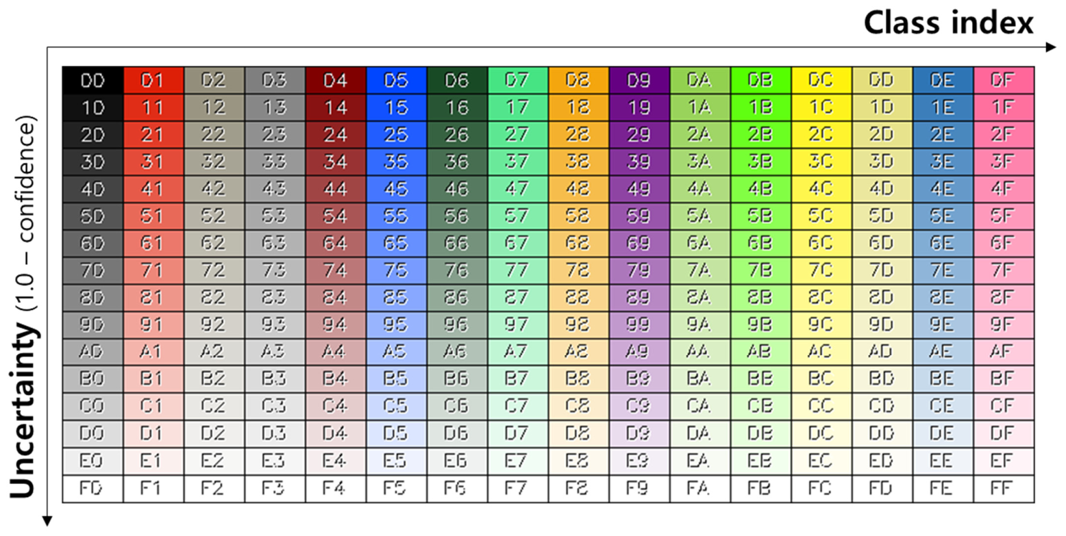
Each pixel in the resulting unified masks is associated with a class index and a confidence level [35]. This information is encoded as a single byte, created by combining the class index (represented in the lower 4 bits) with the confidence level (represented in the higher 4 bits). This encoding allows for a maximum of 16 different classes, with the confidence level expressed across 16 different levels. To maintain consistency with traditional indexed color masks, the confidence level is converted to uncertainty by taking its complement. Figure 12 illustrates the color palette used for the unified dataset in this study.

Figure 12. Color palette for labels of the unified dataset. An entry consists of the upper 4 bits representing the confusion level and the lower 4 bits representing the class index.

3.2. Training a Unified Model

The unified dataset comprises patches from individual datasets, with training masks replaced by harmonized versions. The masks are represented by class indices and uncertainties. Assuming that a mask value consists of c bits (where c = 4 in Section 3.1) representing the confusion level, with the remaining bits designated for the GT class index, the pixel-wise weight W(x) is defined as the complement of the uncertainty U(x) normalized by the maximum available value, as follows:

$$W\left(x\right)=1 - {\displaystyle \frac{U\left(x\right)}{2^c-1}} .$$

(3)

Optimizing parameters θ of ordinary semantic segmentation models involves minimizing the total loss L across all pixel locations, along with a specific regularization term R as follows:

$$\underset{\theta \in \mathsf{\Theta }}{\min }{\displaystyle \sum }_{\left(I, M\right)\in T}L\left(\widehat{M},M\right)+\lambda R\left(\theta \right) ,$$

(4)

where $M$ and $\widehat{M}$ represent the target and predicted logits, respectively.

The pixel-wise weights are utilized in the loss calculation to adjust parameter updates based on confidence levels [36], as illustrated in Equation (5).

$$L\left(\widehat{M},M\right)={\displaystyle \sum }_{x}W\left(x\right)·L\left(\widehat{M}\left(x\right),M\left(x\right)\right)$$

(5)

This loss calculation can be efficiently implemented with minimal lines of code within the MMSegmentation framework (as shown in Listing 1). Crucially, this loss calculation can also be applied to standard semantic masks lacking confidence information, as the upper four bits evaluate to zero under default conditions. After registering the custom module as a new loss class, it can be seamlessly integrated into any decoder configuration by replacing the loss_decode attributes within both the decode_head and auxiliary_head components with the proposed custom loss.

Listing 1. Python implementation of the custom confidence loss module using PyTorch (v2.10.0) and MMSegmentation framework (v1.2.2). The block extract the 4-bit confidence weights and 4-bit sematic labels before evaluating pixel-wise cross-entropy.

from mmseg.registry import MODELS import torch @MODELS.register_module() class MyConfidenceLoss(torch.nn.Module):    def __init__(self, use_mask=False, loss_weight=1.0, loss_name=’MCL’):       super().__init__()       self.loss_weight = loss_weight    def forward(self, cls_score, label, weight=None, avg_factor=None,       reduction_override=None, **kwargs):       # Split the pixel-wise confidence and the associated label       weight = (15 - (label >> 4) & 0xF) / 15.0       label = label & 0xF       # Calculate standard pixel-wise cross-entropy loss       loss = torch.nn.functional.cross_entropy(cls_score, label,          reduction=’none’, ignore_index=255)       # Apply the dynamic pixel-wise confidence weight and global scale       loss = loss * weight       return self.loss_weight * loss

The unified model is trained with a consistent loss function, regardless of the dataset from which a sample originates. However, the metric for selecting the best parameters differs. The model’s performance is assessed using the Mean Intersection over Union (mIoU). We take the average mIoU from all individual datasets as the metric for training the unified model, as we expect it to perform consistently well across all datasets.

3.3. Comparative Evaluation of Universal Performance

The objective of this evaluation is to compare the performance of dedicated models with unified models. Prior to the unification process, all individual datasets were divided into two parts—Part A and Part B—to facilitate 2-fold cross-validation. Performance is evaluated in a cross-part manner: the models from part A are assessed using the dataset from part B and vice versa. This division is carried out without shuffling, ensuring that the locations of the two parts never overlap [37]. For each part, we trained two types of models: dedicated and unified. Specifically, the dedicated models were trained on individual datasets, resulting in three dedicated models, while the unified models were trained on the unified dataset. Within each fold, a random 80:20 split was applied to training pool to divide it into training and validation sets. Consequently, this evaluation framework effectively maintains an overall training, validation, and testing ratio of 4:1:5. Classes with a coverage of less than 1.0% are considered trivial and are excluded from the calculation of the mIoU, such as the background class in both OpenEarthMap and FLAIR.

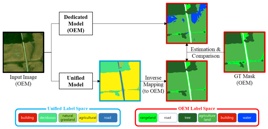
We evaluated the performance of dedicated models versus the unified model in two aspects: intra-dataset and cross-dataset. Intra-dataset performance refers to the evaluation conducted on the same dataset that was used to train a dedicated model. In this context, the original GT mask is available and utilized for evaluation purposes. The output of the unified model is then inverse-mapped to align with the label space. Figure 13 illustrates the overall pipeline of the intra-dataset evaluation within the OpenEarthMap label space.

Figure 13. Intra-dataset validation pipeline for the OpenEarthMap (OEM) label space.

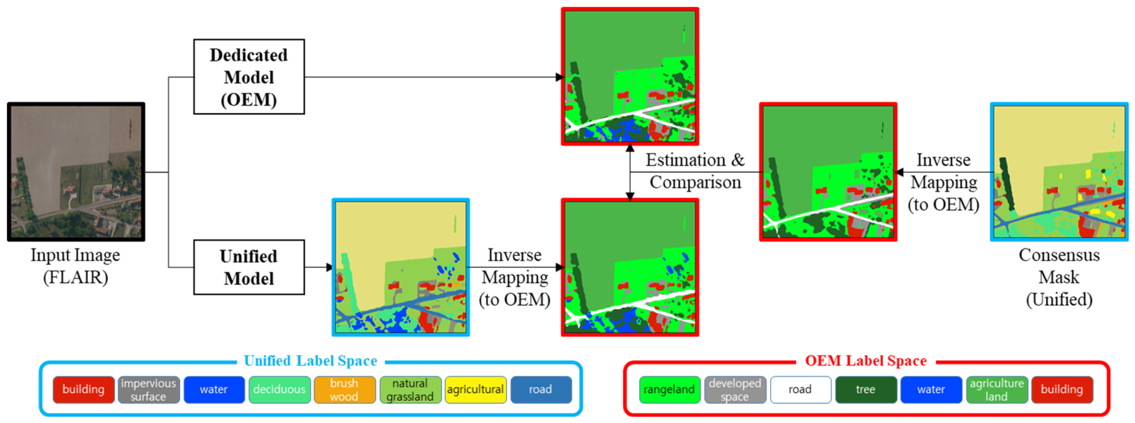
In contrast, cross-dataset performance measures the performance across datasets that were not utilized for training the dedicated model [38]. In this context, we utilize the inverse-mapped unified masks, as the original GT masks for the target label space are unavailable. Although automatically generated from a multi-model consensus rather than being hand-labeled, these masks serve as a viable proxy for actual GT masks to evaluate overall performance on unseen images. Figure 14 illustrates an example of cross-dataset evaluation on a FLAIR image within the OpenEarthMap label space.

Figure 14. Cross-dataset validation pipeline for the OpenEarthMap (OEM) label space.

The unified model inevitably encounters a wider range of scenarios, which may either induce side effects or enhance performance within the specific label space. Intra-dataset estimation demonstrates these effects using images from the same dataset. Conversely, cross-dataset estimation captures performance variations when images from different datasets are used. This evaluation allows us to assess the generalizability of the unified model to images that remain unseen by dedicated models.

To assess the universal effectiveness of the proposed method, we performed extensive benchmarking across a diverse range of prominent semantic segmentation decoder architectures: OCRNet, SegFormer, UperNet, DeepLabV3+, PSPNet, and K-Net. All six architectures are compatible without the need for any internal pipeline modifications. This compatibility arises from a shared foundational approach: regardless of their core mechanisms—whether they use CNN-based dense convolutions (DeepLabV3+ and PSPNet), Transformer-based context aggregations (SegFormer, UperNet, and OCRNet), or dynamic query-based kernel updates (K-Net)—all six decoders maintain the full-resolution spatial grid matrix across the spatial dimensions of height (H) and width (W) when computing the final loss function. As a result, the [H, W] weight map produced by our unified pipeline can be directly multiplied by the loss tensor through simple spatial broadcasting.

In contrast, Mask2Former is a distinct case that does not directly align with the proposed methods. To enhance computational efficiency when working with high-resolution feature maps, Mask2Former avoids the typical full-grid loss calculation. Instead, it employs a framework based on importance sampling that dynamically extracts a sparse 1D array of specific coordinates located near predicted boundaries. This point-sampling step condenses the continuous 2D spatial coordinates into a non-contiguous 1D array, resulting in a [K] dimension. Consequently, the [H, W] spatial weight map becomes isolated and mathematically incompatible with the localized gradient calculation utilized by Mask2Former, unless extensive architectural modifications are made. Consequently, Mask2Former was excluded from the unified model evaluation to maintain focus on the six architectures with native spatial loss compatibility. It nonetheless remains a viable candidate for the base model architecture in consensus-based probability estimation, as this initial unification phase is independent of the weight-map-based loss calculations used during final model training.

Under the 2-fold cross-validation setup, the MMI ensemble was benchmarked using the K-Net architecture with a Swin Transformer-Base backbone. Beyond their primary role in generating the unified dataset, MMIs can also produce direct ensemble results through majority voting. Since these MMIs are trained solely on their respective native datasets, they have not encountered cross-domain imagery, mimicking dedicated models. Consequently, this benchmark allows us to evaluate performance improvements considering collective intelligence in both intra- and cross-dataset settings.

The partitioning method is an effective way to assess generalization; however, it can be quite strict since only 50% of the data is used to train the model, potentially leading to underfitting. To address this issue, we also conducted a performance evaluation without partitioning for a selected model architecture to better understand the model’s realistic and qualitative performance. In this approach, the dataset was partitioned into a 20% test set and an 80% training set. To evaluate generalization performance, data shuffling was omitted. Within the training partition, 20% was reserved for validation to determine the optimal metric parameters, leading to an effective split of 64% for training, 16% for validation, and 20% for testing.

Finally, to verify the statistical significance of class-wise improvements across diverse network architectures, the Wilcoxon signed-rank test was conducted for both the 2-fold cross-validation and holdout validation, with the intra- and cross-dataset settings evaluated separately [39]. Within each of these four distinct evaluation blocks, paired class IoU values from a dedicated model and the unified model served as individual samples. We estimated the p-value and Rank-Biserial Correlation (RBC) across individual network architectures and obtained the overall estimates.

4. Results

4.1. Selection of Base Model Architecture

We evaluated the performance of different model architectures through dedicated models to determine a suitable architecture for dataset fusion. Table 3 summarizes the performance of these dedicated models, evaluated using a random 80/20 train-validation split. Additionally, it includes the number of parameters, which indicates the numerical complexity of each model.

Table 3. Comparison of performance and complexity of dedicated models across three datasets: OpenEarthMap (OEM), FLAIR, and AI-Hub cloud (CLD).

Model Architecture			Model Performance (mIoU)
Decoder	Backbone	Params	OEM	FLAIR	CLD	Mean
OCRNet	HRNet-W18	10 M	59.6	71.6	79.5	70.2
SegFormer	MiT-B2	24 M	79.4	85.1	88.3	84.3
UperNet	Swin-T	60 M	79.7	85.4	86.1	83.7
DeepLabv3+	ResNet101	63 M	82.2	82.4	81.0	81.9
PSPNet	ResNet101	68 M	72.1	81.2	80.9	78.1
OCRNet	HRNet-w48	70 M	71.3	79.6	80.5	77.1
SegFormer	MiT-B5	82 M	81.9	88.1	88.8	86.3
UperNet	Resnet101	86 M	76.1	86.1	80.5	80.9
UperNet	UniRepLKNet-B	104 M	83.3	88.7	89.6	87.2
Mask2Former	Swin-B	107 M	81.6	86.7	83.7	84.0
Mask2Former	ConvNeXt-B	108 M	80.7	86.5	84.0	83.7
K-Net	Swin-B	109 M	83.5	87.7	85.6	85.6
UperNet	Swin-B	121 M	82.5	88.0	89.0	86.5
UperNet	ConvNeXt-B	122 M	80.3	86.7	89.3	85.4
K-Net	ViT-CoMer-B	140 M	77.5	85.4	88.5	83.8
Mask2Former	ViT-CoMer-B	145 M	77.9	85.4	86.2	83.2
Mask2Former	Swin-L	215 M	81.9	87.1	83.4	84.1
K-Net	Swin-L	223 M	84.7	88.9	88.5	87.4

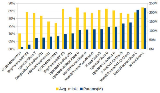
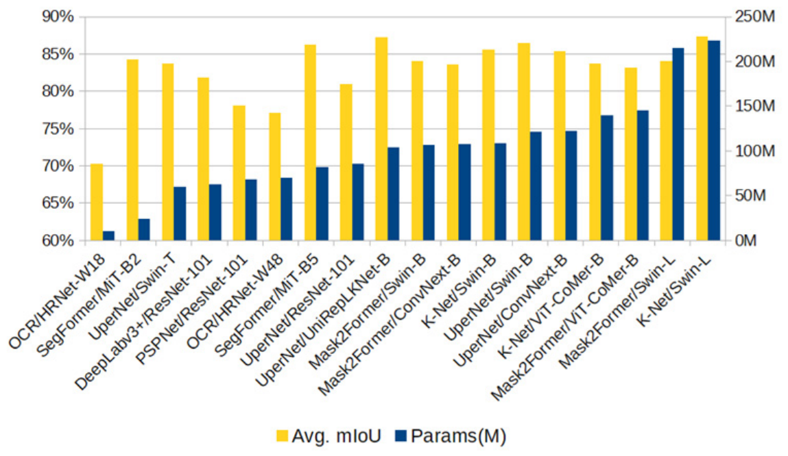
Figure 15 illustrates the average performance of various network architectures along with their corresponding number of parameters, following a similar evaluation approach to [40]. The combination of K-Net and the Swin Transformer achieved the highest performance. Although UperNet with UniRepLKNet-B achieved a higher average score compared to K-Net with Swin-B, it was excluded due to its relatively high performance variance across datasets, leading us to select the latter instead, as it offers an optimal balance between performance and complexity supported by its parameter size, decoder properties, and a highly verified backbone.

Figure 15. Average mean Intersection over Union (mIoU) and the number of parameters (M) across different network architectures for dedicated models.

4.2. Generation of the Unified Dataset

The unified dataset was created by combining three individual datasets using the proposed method. The images included are the same as those in the original individual datasets. The associated training masks have been converted to unified masks, with the lower 4 bits representing class indices and the upper 4 bits indicating the level of confusion. This approach ensures compatibility with the original class masks, where the upper bits are set to 0, indicating that there is no confusion.

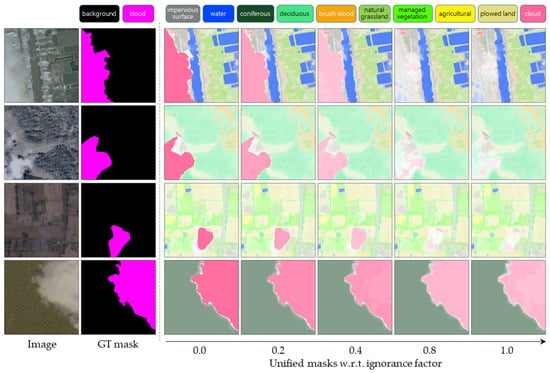
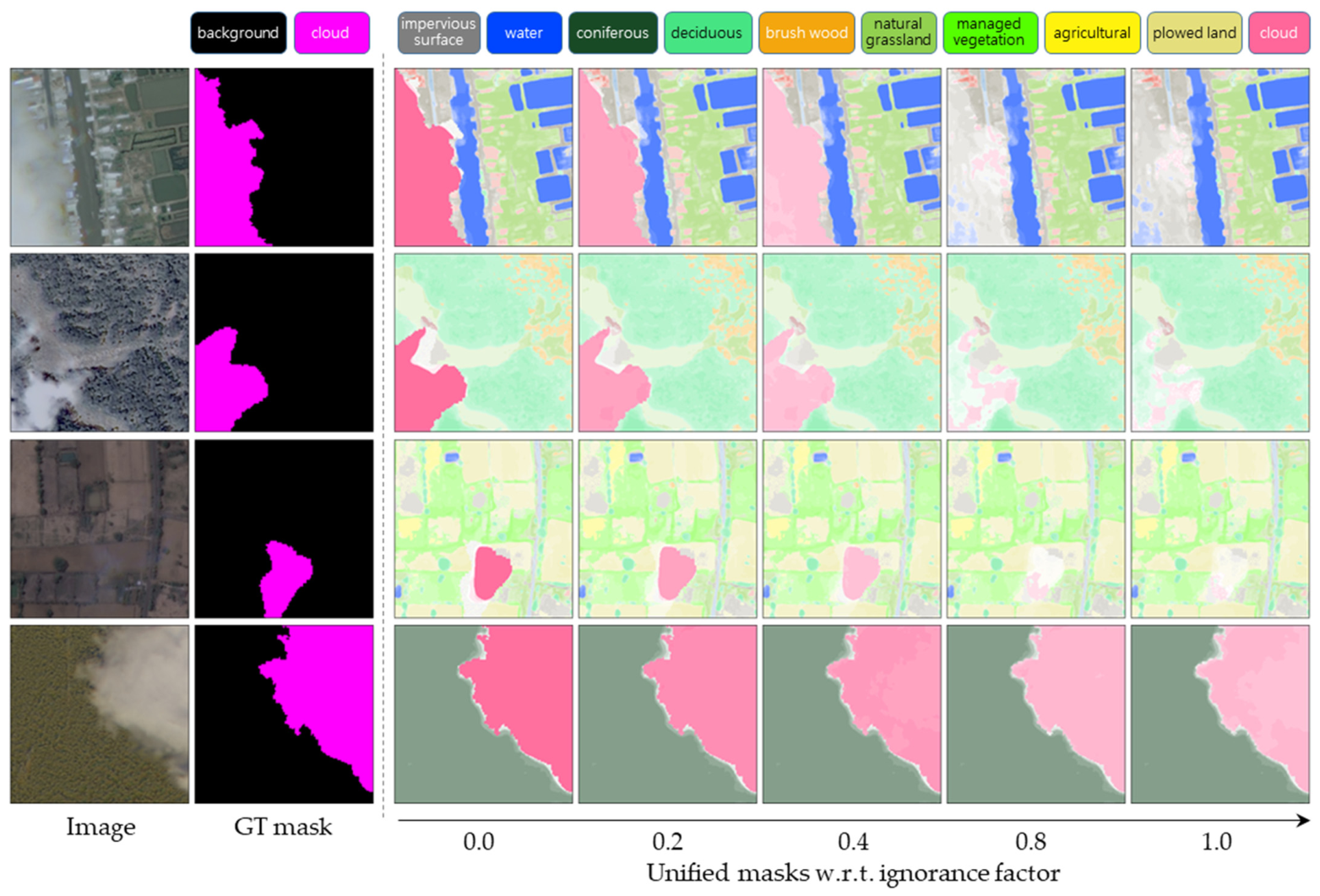
The resulting unified masks generated with varying ignorance factors of Equation (1) are exemplified in Figure 16. A value of 1.0 implies no intervention, causing each pixel-wise probability to have an equal effect despite the absence of dataset prior knowledge. Under this setting, cloud regions largely vanish, increasing confusion and hindering cloud class learning. Conversely, a value of 0.0 ensures that the AIHub cloud dataset has an absolute influence, producing vivid cloud masks that reinforce cloud class learning. To accommodate the inherently ambiguous states where clouds and other classes coexist, the value is fine-tuned to 0.2 to achieve an optimal compromise.

Figure 16. Qualitative comparison of unified masks under different ignorance factors. Each row shows an example. From left to right: the input image, the ground-truth (GT) mask, and the unified masks with the ignorance factor increasing from 0.0 to 1.0.

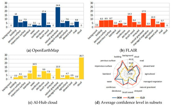
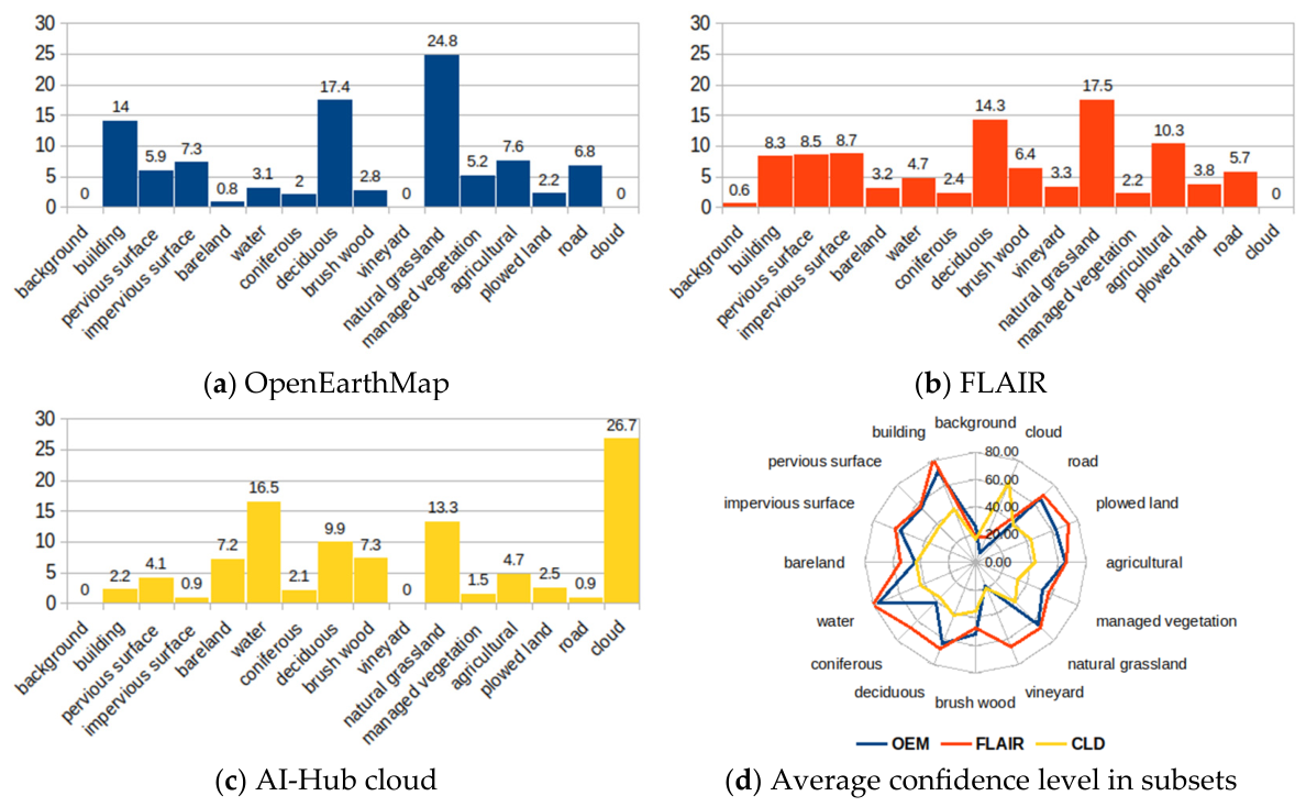
All individual datasets have been combined into a unified dataset, but they are still managed as separate derived subsets. We refer to a derived subset by the name of its original dataset. Figure 17a–c illustrates the class frequency distribution within these derived subsets. Notably, OpenEarthMap and FLAIR had similar class compositions, whereas the cloud class was unique to the AI-Hub cloud, and the vineyard class was exclusive to FLAIR. Additionally, the presence of the background class was negligible. Figure 17d illustrates the average confidence level (%) for each class across derived subsets. It demonstrates how strongly each individual dataset impacts a class, which influences the unified model’s loss calculation and parameter updates.

Figure 17. Class frequency distributions and average confidence levels in derived subsets: (a–c) class frequency distributions; (d) average confidence levels.

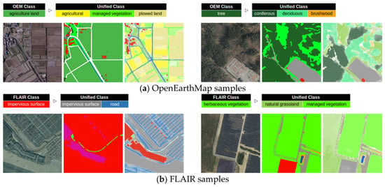
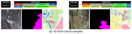
Figure 18 illustrates a comparison between the original individual class masks and the unified class masks, along with their corresponding images. It demonstrates that some original classes have been subdivided into more detailed categories. Notably, in the cloud dataset, the background class corresponds to all classes except for the cloud class.

Figure 18. Representative examples comparing original and unified masks across different datasets. Left, center, and right panels display the image, original GT mask, and unified mask, respectively. Top legends illustrate the corresponding class mapping relationships.

In the unified mask, confidence levels are represented by color saturation: pixels that are fully confident retain their bright class colors, while areas with no confidence fade to pure white. This is particularly evident in Figure 18c, where cloud colors often appear muted. This muted appearance may be due to the inherent ambiguity of clouds themselves, as well as the tendency of models across different datasets to classify them into various categories.

4.3. Results on 2-Fold Cross Validation

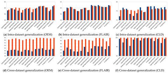
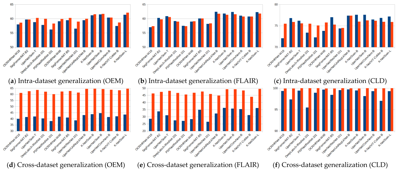
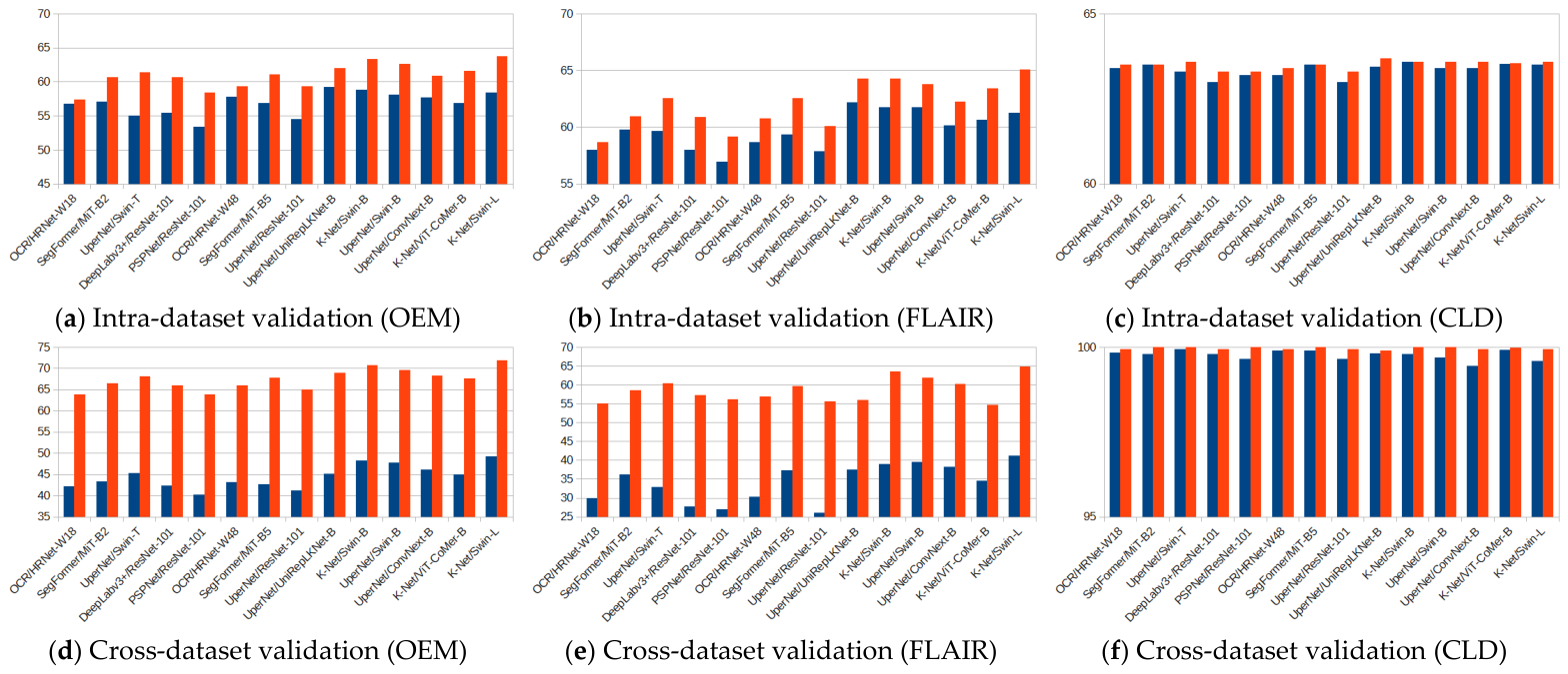
Table 4 compares the performance of dedicated models with that of a unified model. The performance metrics presented are averages of the models’ performance across Part A and Part B. Each derived subset is evaluated using different segmentation architectures. Figure 19 summarizes the evaluation results from Table 4, highlighting both intra-dataset and cross-dataset generalization.

Table 4. The 2-fold cross-validation performance comparison (mIoU) between dedicated models of each label space and the unified model across OpenEarthMap (OEM), FLAIR (FLR), and AI-Hub cloud (CLD) subsets.

Network Architecture (Decoder/Backbone)	OpenEarthMap Label Space						FLAIR Label Space						AI-Hub Cloud Label Space
	Dedicated Model			Unified Model			Dedicated Model			Unified Model			Dedicated Model			Unified Model
	OEM	FLR	CLD	OEM	FLR	CLD	OEM	FLR	CLD	OEM	FLR	CLD	OEM	FLR	CLD	OEM	FLR	CLD
OCR/HRNet-W18	58.0	47.9	32.3	58.6	68.2	54.1	36.6	57.0	20.6	50.5	57.4	42.1	99.2	99.5	72.1	99.9	100.0	75.5
SegFormer/MiT-B2	59.7	49.6	33.3	59.7	70.2	55.0	43.7	60.3	23.8	51.9	59.8	43.1	96.9	97.9	76.8	99.9	100.0	75.9
UperNet/Swin-T	58.8	49.2	34.8	60.3	71.5	55.6	41.8	60.9	20.5	52.6	60.6	43.7	99.1	99.8	76.2	100.0	100.0	75.6
DeepLabv3+/ResNet-101	57.8	47.7	32.9	60.0	69.7	54.6	39.2	59.2	15.8	51.1	59.0	42.4	98.0	93.0	73.4	100.0	100.0	75.5
PSPNet/ResNet-101	56.2	45.3	31.1	58.3	66.6	53.6	37.2	57.5	17.1	49.4	57.4	41.9	99.0	98.9	72.3	100.0	100.0	75.1
OCR/HRNet-W48	59.1	48.8	34.7	59.9	69.9	54.7	38.6	59.0	18.1	51.0	59.1	42.8	99.7	99.7	73.8	99.9	100.0	75.8
SegFormer/MiT-B5	59.5	49.6	32.5	60.3	70.4	55.0	44.7	60.1	25.0	52.4	60.1	43.1	98.0	98.9	77.0	99.9	100.0	75.3
UperNet/ResNet-101	56.5	47.5	30.1	59.0	69.3	53.6	37.0	58.2	16.1	50.3	58.4	41.6	99.4	99.7	74.4	100.0	100.0	74.5
UperNet/UniRepLKNet-B	59.5	51.2	35.0	60.0	72.8	56.2	41.2	62.4	23.5	48.2	61.7	41.6	99.6	99.9	77.4	99.9	100.0	76.5
K-Net/Swin-B	61.2	51.4	36.2	61.6	72.8	56.4	46.3	61.8	26.2	54.5	61.4	44.2	99.2	99.8	77.6	99.9	100.0	76.0
UperNet/Swin-B	61.5	52.8	36.6	61.7	72.7	56.1	45.3	62.4	26.2	54.7	61.6	43.9	97.0	99.3	77.6	100.0	100.0	76.3
UperNet/ConvNext-B	60.4	50.1	33.0	60.4	71.8	55.8	44.9	61.1	25.9	53.0	60.8	43.9	99.1	99.5	76.5	99.9	100.0	76.2
K-Net/ViT-CoMer-B	57.4	49.8	34.2	58.7	71.4	55.2	39.8	60.8	22.7	47.3	60.8	40.6	96.4	97.7	76.9	100.0	100.0	76.0
K-Net/Swin-L	61.4	51.2	35.7	62.1	73.0	56.3	46.0	62.3	26.3	54.9	61.8	44.2	98.8	99.8	77.2	100.0	100.0	75.9
Average	59.1	49.4	33.7	60.0	70.7	55.2	41.6	60.2	22.0	51.6	60.0	42.8	98.5	98.8	75.7	99.9	100.0	75.7

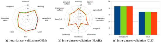
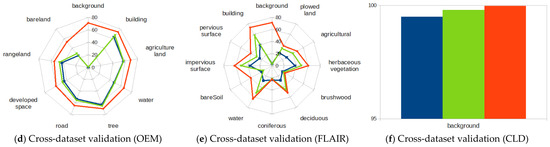
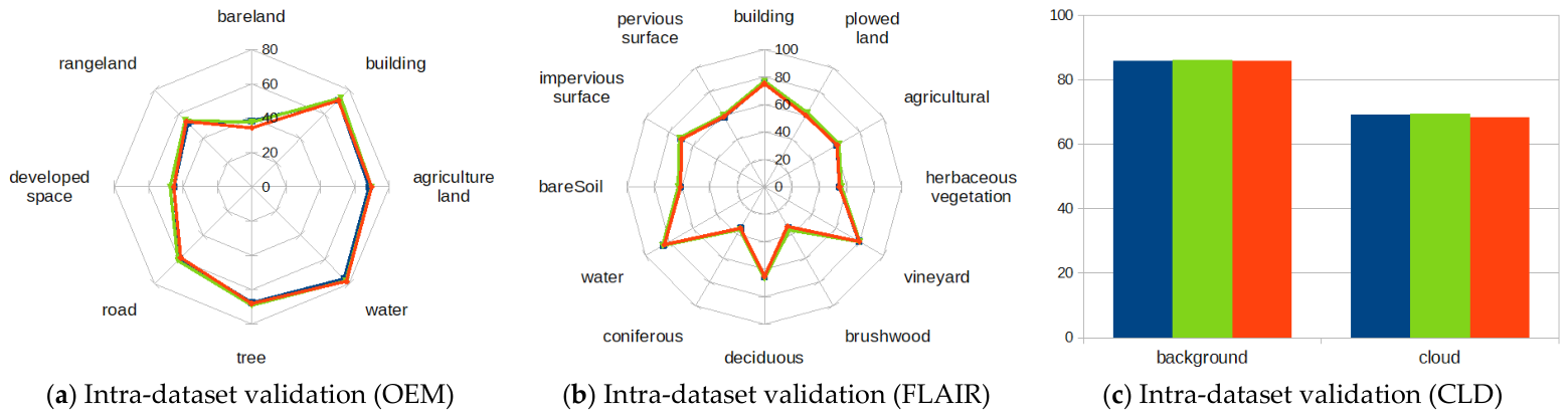
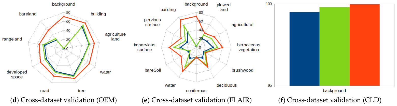
Figure 19. Performance comparison between dedicated (blue) and unified (red) models across OpenEarthMap (OEM), FLAIR, and AI-Hub cloud (CLD) label spaces under 2-fold cross-validation: (a–c) intra-dataset and (d–f) cross-dataset generalization.

For the dedicated models of OpenEarthMap and FLAIR, the intra-dataset performance (blue bars in Figure 19a vs. Figure 19b) was consistently higher than the cross-dataset performance (blue bars in Figure 19d vs. Figure 19e). Specifically, across all evaluated network architectures, the average mIoU gaps between these two evaluation settings were 17.5% and 28.4%, respectively. In contrast, for the AI-Hub cloud dataset, a direct comparison between intra- and cross-dataset generalization was not feasible due to the absence of cloud classes in the other datasets.

Within the OpenEarthMap label space, unified models consistently outperform dedicated models in both intra- and cross-dataset scenarios, irrespective of the network architecture. Specifically, unified models yield a modest average improvement of 1.0% in intra-dataset generalization (blue vs. red bars in Figure 19a), which expands substantially to 21.4% in cross-dataset performance (Figure 19d). Similarly, in the FLAIR dataset label space, while the average intra-dataset performance of unified models decreases marginally by 0.2% (Figure 19b), their cross-dataset performance improves substantially across all cases, yielding an average increase of 15.4% (Figure 19e).

For the AI-Hub cloud dataset, the alteration in intra-dataset performance is inconsistent (blue vs. red bars Figure 19c), yielding a marginal average increase of 0.1%. Conversely, cross-dataset generalization performance consistently improves across all cases, with an average increment of 1.3% (Figure 19f). This trend implies that the unified models effectively mitigate the misclassification of non-cloud areas as cloud cover.

Figure 20 shows class-wise IoU for dedicated models, the MMI ensemble, and the unified model using the K-Net with the Swin Transformer-Base architecture, and Table 5 summarizes mIoU for intra- and cross-dataset settings across the respective label spaces. The MMI ensemble showed marginal improvements in intra-dataset validation (1.3% for FLAIR) and cross-dataset validation (2.7% for OEM and 0.8% for FLAIR). However, the unified model’s cross-dataset improvements substantially outperformed those of the MMI ensemble, reaching 20.8% for OEM and 13.1% for FLAIR.

Figure 20. Class-wise IoU comparison between dedicated (blue), MMI ensemble (green), and unified (red) models across OpenEarthMap, FLAIR, and AI-Hub cloud label spaces: (a–c) intra- and (d–f) cross-dataset validation (K-Net with Swin-Transformer-Base).

Table 5. Comparison of 2-fold cross-validation performance (mIoU) among dedicated models, MMI ensemble, and the unified model across OpenEarthMap, FLAIR, and AI-Hub cloud subsets.

Label Space	OpenEarthMap		FLAIR		AI-Hub Cloud
	Intra-Dataset	Cross-Dataset	Intra-Dataset	Cross-Dataset	Intra-Dataset	Cross-Dataset
Dedicated model	61.4	43.8	61.8	36.3	77.6	99.5
MMI ensemble	61.3	46.5	63.1	37.1	77.8	99.8
Unified model	61.8	64.6	61.4	49.4	77.0	100.0

4.4. Results on Hold-Out Validation

Table 6 presents a performance comparison based on holdout validation. Similar to the 2-fold cross-validation scenario, we compared the dedicated model for each label space with the unified model that produces inverse-mapped outputs. Consistent with the 2-fold cross-validation setting, this evaluation also involved a comparative analysis of various segmentation architectures.

Table 6. Holdout validation performance comparison (mIoU) between dedicated models of each label space and the unified model across OpenEarthMap (OEM), FLAIR (FLR), and AI-Hub cloud (CLD) subsets.

Network Architecture (Decoder/Backbone)	OpenEarthMap Label Space						FLAIR Label Space						AI-Hub Cloud Label Space
	Dedicated Model			Unified Model			Dedicated Model			Unified Model			Dedicated Model			Unified Model
	OEM	FLR	CLD	OEM	FLR	CLD	OEM	FLR	CLD	OEM	FLR	CLD	OEM	FLR	CLD	OEM	FLR	CLD
OCR/HRNet-W18	56.8	47.9	36.5	57.4	68.0	59.7	39.0	58.0	21.1	55.1	58.7	55.2	99.7	100.0	63.4	99.9	100.0	63.5
SegFormer/MiT-B2	57.1	49.4	37.4	60.7	70.4	62.7	42.2	59.8	30.5	58.1	61.0	59.0	99.6	100.0	63.5	100.0	100.0	63.5
UperNet/Swin-T	55.1	50.1	40.6	61.4	72.4	64.0	40.5	59.7	25.5	60.6	62.6	60.5	99.9	100.0	63.3	100.0	100.0	63.6
DeepLabv3+/ResNet-101	55.5	48.3	36.4	60.7	70.2	61.7	38.3	58.0	17.2	57.6	60.9	57.0	99.7	99.9	63.0	99.9	100.0	63.3
PSPNet/ResNet-101	53.4	45.4	35.1	58.5	67.3	60.5	37.3	57.0	16.8	56.1	59.2	56.5	99.5	99.8	63.2	100.0	100.0	63.3
OCR/HRNet-W48	57.8	48.3	38.3	59.4	70.5	61.4	38.2	58.7	22.5	57.3	60.8	56.6	99.8	100.0	63.2	99.9	100.0	63.4
SegFormer/MiT-B5	56.9	49.5	36.0	61.1	71.8	63.8	44.2	59.4	30.7	59.0	62.6	60.3	99.8	100.0	63.5	100.0	100.0	63.5
UperNet/ResNet-101	54.6	47.8	34.6	59.4	69.9	60.2	36.2	57.9	16.2	56.5	60.1	54.9	99.5	99.8	63.0	99.9	100.0	63.3
UperNet/UniRepLKNet-B	59.3	51.4	39.0	62.0	73.8	64.3	43.5	62.2	31.6	55.8	64.3	56.3	99.6	100.0	63.4	99.8	100.0	63.7
K-Net/Swin-B	58.9	51.8	44.8	63.4	74.4	67.1	45.8	61.8	32.3	63.0	64.3	64.1	99.6	100.0	63.6	100.0	100.0	63.6
UperNet/Swin-B	58.1	52.4	43.1	62.6	73.5	65.7	46.9	61.8	32.5	61.5	63.8	62.3	99.4	100.0	63.4	100.0	100.0	63.6
UperNet/ConvNext-B	57.7	50.7	41.5	60.9	72.4	64.2	44.0	60.2	32.5	59.9	62.3	60.6	98.9	100.0	63.4	99.9	100.0	63.6
K-Net/ViT-CoMer-B	56.9	50.5	39.5	61.6	71.9	63.3	41.5	60.6	27.9	54.2	63.5	55.2	99.8	100.0	63.5	100.0	100.0	63.6
K-Net/Swin-L	58.5	52.9	45.6	63.8	75.5	68.5	47.3	61.3	35.3	64.3	65.1	65.6	99.2	100.0	63.5	99.9	100.0	63.6
Average	56.9	49.7	39.2	60.9	71.6	63.4	41.8	59.7	26.6	58.5	62.1	58.9	99.6	100.0	63.4	99.9	100.0	63.5

Figure 21 summarizes the evaluation results from Table 6, highlighting both intra- and cross-dataset validation. Both OpenEarthMap and FLAIR dedicated models exhibited higher intra-dataset results than cross-dataset results, mirroring the 2-fold cross-validation trend (blue bars in Figure 21a vs. Figure 21d, and Figure 21b vs. Figure 21e). However, the performance gap narrowed from 17.5% to 12.4% for OpenEarthMap and from 28.4% to 25.6% for FLAIR.

Figure 21. Performance comparison (mIoU) between dedicated (blue) and unified (red) models across OpenEarthMap (OEM), FLAIR, and AI-Hub cloud (CLD) label spaces under holdout validation: (a–c) intra-dataset and (d–f) cross-dataset validation.

The performance advantage of the unified model over dedicated counterparts is further amplified within the holdout validation framework. For intra-dataset evaluation, transitioning from 2-fold cross-validation to holdout validation expands the performance gap from 1.0% to 4.0% for OpenEarthMap (blue vs. red bars in Figure 21a) and from −0.2% to 2.3% for FLAIR (Figure 21b).

Likewise, in cross-dataset scenarios, holdout validation revealed a more pronounced performance advantage of 23.0% for OpenEarthMap (blue vs. red bars in Figure 21d) and 24.5% for FLAIR (Figure 21e), surpassing the 2-fold cross-validation benchmarks of 21.4% and 15.4%, respectively. Within the AI-Hub cloud label space, while holdout validation ensures architectural consistency with a marginal average gain of 0.1% (Figure 21c), 2-fold cross-validation results remain highly variable despite registering the same average improvement of 0.1% (Figure 19c).

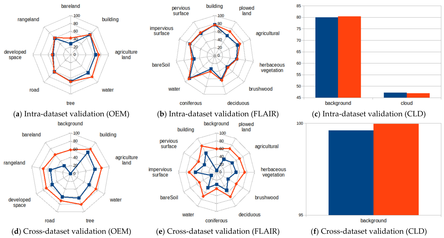
Figure 22 presents a comparison of the class-wise IoU between dedicated models and the unified model using the K-Net with Swin-Transformer-Large across each label space. In the OpenEarthMap label space, intra-dataset validation revealed a substantial 14.6% IoU improvement for the bareland class, alongside an average increase of 4.0% across other classes (blue vs. red lines in Figure 22a). This trend intensified in cross-dataset validation (Figure 22d), where the background class IoU surged by 58.7%, and the remaining classes achieved a higher average improvement of 18.2%.

Figure 22. Class-wise IoU comparison between dedicated (blue) and unified (red) models across OpenEarthMap, FLAIR, and AI-Hub cloud label spaces: (a–c) intra- and (d–f) cross-dataset validation (K-Net with Swin-Transformer-Large).

In the FLAIR label space, intra-dataset validation yielded substantial improvement for the plowed land class, showing gain of 12.3%. In contrast, the average improvement for the remaining classes was limited to 2.9% (blue vs. red lines in Figure 22b). The cross-dataset validation demonstrated a more pronounced improvement, yielding a 55.0% gain for the background class and a 22.5% average across the remaining classes (Figure 22e).

The AI-Hub cloud dataset registers mixed performance shifts under intra-dataset evaluation, where the background class exhibits an average increase of 0.4% while the cloud class decreases by 0.2% (blue vs. red bars in Figure 22c). In cross-dataset validation, a 0.4% rise is observed for the background class (Figure 22f). Overall, both outcomes confirm a consistent improvement in preventing false cloud detections, with negligible impact on cloud-to-cloud classification performance.

4.5. Statistical Analysis of Performance Improvements

Table 7 and Table 8 summarize the statistical validation results. For the 2-fold cross-validation setup (Table 7), the intra-dataset validation yielded an average p-value of 0.017, which falls below the conventional significance level of 0.05, indicating a statistically significant difference between the models. However, the corresponding RBC was 0.11, representing a weak effect size. Under the same validation setup, the cross-dataset analysis yielded a highly significant aggregate p-value (p < 0.0001) and a near-perfect average RBC of 0.98, confirming a strong and consistent treatment effect across network architectures.

Table 7. Wilcoxon signed-rank test of performance gains for unified models in 2-fold cross-validation setup across various network architectures.

Network Architecture (Decoder/Backbone)	Intra-Dataset Validation					Cross-Dataset Validation
	Average of Class-Wise IoUs			Wilcoxon Test		Average of Class-Wise IoUs			Wilcoxon Test
	Dedicated	Unified	Gain	p-Value	RBC	Dedicated	Unified	Gain	p-Value	RBC
OCR/HRNet-W18	58.8	59.5	0.7	0.016	0.42	36.6	55.0	18.4	3.1 × 10−15	0.99
SegFormer/MiT-B2	61.6	61.3	−0.3	0.113	−0.28	39.7	56.2	16.5	1.1 × 10−14	0.97
UperNet/Swin-T	61.6	61.9	0.3	0.995	0.00	38.6	57.0	18.4	4.3 × 10−15	0.99
DeepLabv3+/ResNet-101	60.0	60.8	0.8	0.005	0.49	35.7	55.6	19.9	2.7 × 10−15	0.99
PSPNet/ResNet-101	58.4	59.4	1.0	0.001	0.58	34.9	54.2	19.3	2.4 × 10−15	0.99
OCR/HRNet-W48	60.4	60.9	0.5	0.014	0.43	37.1	55.8	18.7	3.4 × 10−15	0.99
SegFormer/MiT-B5	61.5	61.6	0.1	0.891	0.03	40.2	56.4	16.1	2.0 × 10−14	0.96
UperNet/ResNet-101	59.1	60.1	1.0	0.016	0.42	34.8	54.9	20.1	2.9 × 10−15	0.99
UperNet/UniRepLKNet-B	62.7	62.5	−0.3	0.062	−0.32	41.2	57.4	16.2	1.3 × 10−14	0.96
K-Net/Swin-B	63.1	62.8	−0.2	0.134	−0.26	42.1	58.0	15.9	4.4 × 10−14	0.95
UperNet/Swin-B	63.5	63.0	−0.5	0.012	−0.44	42.2	57.9	15.7	8.1 × 10−15	0.98
UperNet/ConvNext-B	62.3	62.1	−0.2	0.335	−0.17	40.8	57.2	16.5	2.1 × 10−14	0.96
K-Net/ViT-CoMer-B	61.0	61.4	0.4	0.087	0.30	40.0	56.4	16.4	2.2 × 10−15	0.98
K-Net/Swin-L	63.4	63.2	−0.1	0.398	−0.15	41.9	58.2	16.2	7.5 × 10−15	0.98
Average	61.24	61.47	0.23	0.017	0.11	39.00	56.45	17.45	1.1 × 10−186	0.98

Table 8. Wilcoxon signed-rank test of performance gains for unified models in holdout validation setup across various network architectures.

Network Architecture (Decoder/Backbone)	Intra-Dataset Validation					Cross-Dataset Validation
	Average of Class-Wise IoUs			Wilcoxon Test		Average of Class-Wise IoUs			Wilcoxon Test
	Dedicated	Unified	Gain	p-Value	RBC	Dedicated	Unified	Gain	p-Value	RBC
OCR/HRNet-W18	58.0	58.7	0.6	0.838	−0.06	38.2	60.9	22.7	2.3 × 10−13	1.00
SegFormer/MiT-B2	59.1	61.1	2.0	0.076	0.45	42.1	63.8	21.7	2.3 × 10−13	1.00
UperNet/Swin-T	58.3	62.2	4.0	0.004	0.70	41.1	65.6	24.5	2.3 × 10−13	1.00
DeepLabv3+/ResNet-101	57.5	61.1	3.5	0.000	0.95	37.0	62.9	25.9	2.3 × 10−13	1.00
PSPNet/ResNet-101	56.2	59.3	3.1	0.000	0.89	35.7	61.5	25.8	2.3 × 10−13	1.00
OCR/HRNet-W48	58.8	60.5	1.7	0.060	0.47	38.8	62.7	23.9	2.3 × 10−13	1.00
SegFormer/MiT-B5	58.8	62.1	3.3	0.001	0.80	42.4	65.0	22.6	2.3 × 10−13	1.00
UperNet/ResNet-101	57.1	60.2	3.0	0.000	0.83	35.6	61.7	26.0	2.3 × 10−13	1.00
UperNet/UniRepLKNet-B	61.3	63.4	2.1	0.003	0.69	45.1	66.0	20.8	2.3 × 10−13	1.00
K-Net/Swin-B	60.9	63.9	3.0	0.000	0.86	45.6	68.3	22.7	2.3 × 10−13	1.00
UperNet/Swin-B	60.5	63.3	2.8	0.002	0.72	45.7	66.9	21.2	2.3 × 10−13	1.00
UperNet/ConvNext-B	59.5	61.9	2.4	0.003	0.71	44.2	65.5	21.3	2.3 × 10−13	1.00
K-Net/ViT-CoMer-B	59.5	62.8	3.3	0.000	0.99	43.4	64.7	21.3	2.3 × 10−13	1.00
K-Net/Swin-L	60.4	64.5	4.0	0.000	0.96	47.2	69.5	22.3	2.3 × 10−13	1.00
Average	59.02	61.79	2.77	1.1 × 10−27	0.73	41.59	64.63	23.04	2.8 × 10−100	1.00

Regarding the hold-out validation setup presented in Table 8, the intra-dataset validation showed a highly significant aggregate p-value (p < 0.0001) and an average RBC of 0.73, which indicates a strong statistical relationship. In the corresponding cross-dataset validation, the aggregate p-value was also highly significant (p < 0.0001), with the RBC value remaining at 1.00 across all evaluated network architectures, confirming a maximum possible effect size and a clear performance divergence.

5. Discussion

Our discussion centers on the efficacy of leveraging pixel-wise class probabilities derived from MMIs to harmonize heterogeneous remote sensing datasets. A key strength of this methodology lies in its capacity to expand the unified dataset’s label space beyond any single constituent framework of OpenEarthMap, FLAIR, and AI-Hub cloud dataset. In particular, the third dataset was selected for its practical utility. While most existing land-cover datasets rely exclusively on cloud-free imagery, real-world satellite observations frequently contain cloud-obscured areas that cause significant misclassifications. Even when employing a conventional two-step approach—performing cloud detection prior to land-cover segmentation—ambiguities inevitably persist at the boundaries between cloudy and clear regions. Despite this highly heterogeneous and challenging setup, our approach offers an effective strategy by directly integrating cloud recognition capabilities within the core land-cover segmentation model.

Within the framework of dataset unification, pixel-wise class probability estimation functions as an essential regularization mechanism. Quantifying label confidence via the collective predictions of MMIs—and subsequently incorporating these values into pixel-wise parameter-update weights—enables the system to effectively suppress the propagation of uncertain or erroneous information. Consequently, this design structurally resolves the fundamental contradictions inherent in merging disparate GT definitions.

Our dual-validation protocol highlights the distinct robustness of the unified model against different dataset label spaces. In intra-dataset validation, class inverse-mapping is simply used to project the unified label space back into each individual label space, ensuring a direct and structurally fair comparison on native images. In cross-dataset validation, we aimed to address the lack of native annotations on target images. While the dedicated models are evaluated in a strict zero-shot setting, unified models are trained on cross-domain images using ensemble-refined training masks derived from the corresponding GT masks. Mapping these test-set masks back to their respective individual label spaces establishes a consistent benchmark for comparison.

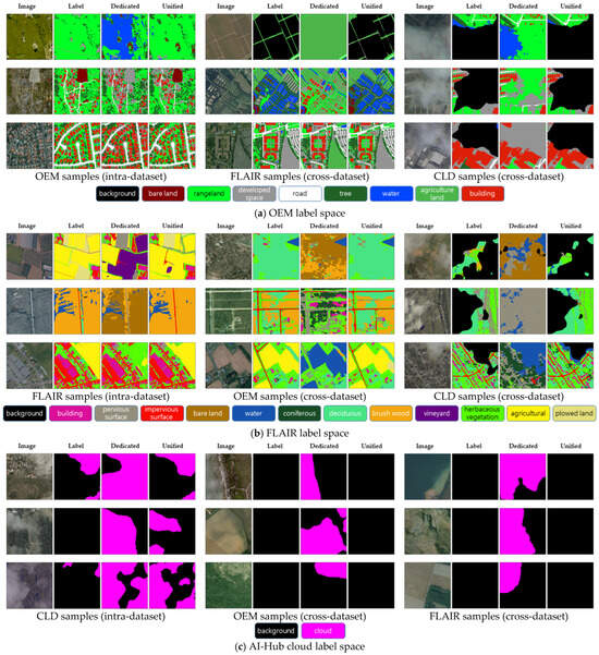
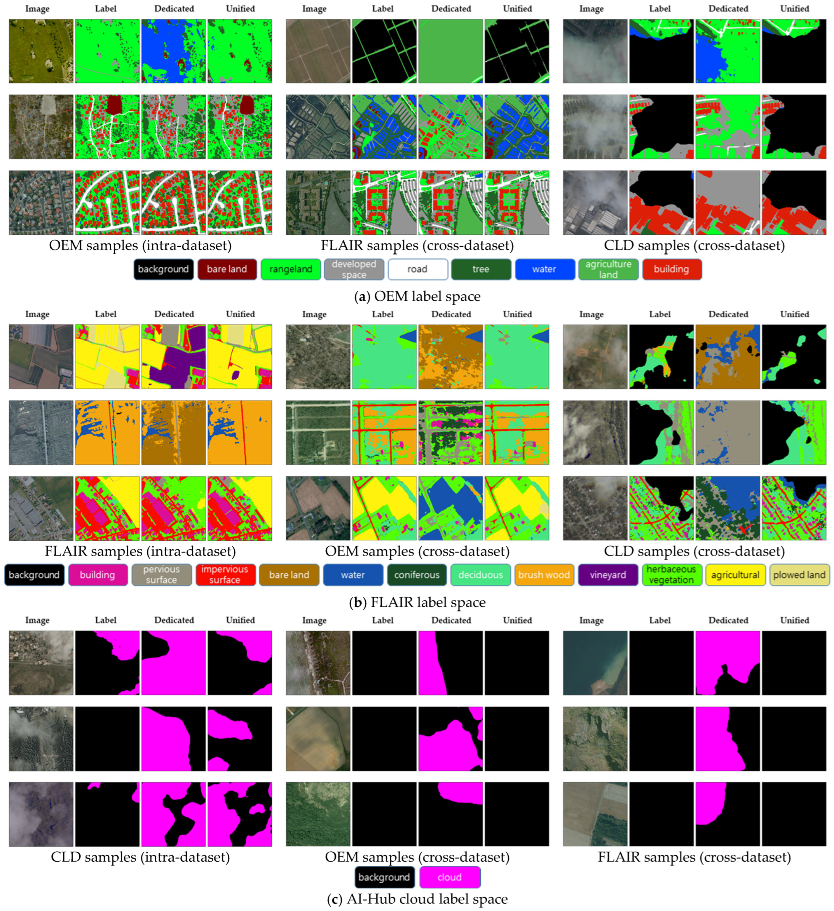
In the two-fold validation setting, the unified model demonstrated performance on par with the dedicated models in intra-dataset evaluation, while exhibiting a substantial increase in generalization during cross-dataset validation. This suggests that the proposed label unification approach enhances robustness without compromising baseline performance, even under limited training data conditions. In the holdout scenario, both intra- and cross-dataset evaluations demonstrated significant improvements, indicating that the heterogeneous GT masks were effectively reconciled to elevate overall performance. Despite being evaluated across three distinct label spaces, the unified model remains a single entity that accommodates a broader label taxonomy and demonstrates improved robustness to unseen imagery. The visual improvements are qualitatively demonstrated in Figure 23, which compares the inference results of both models, which share the same K-Net with Swin-Transformer-Large backbone, alongside the corresponding input images and GT masks. In addition to an overall stabilized inference in the unified models’ results, the capability to recognize unseen objects—such as vineyards and clouds—as background notably improved.

Figure 23. Qualitative comparison of dedicated and unified models based on the K-Net with Swin-Transformer-Large architecture across (a) OEM, (b) FLAIR, and (c) CLD label spaces. Each section contains three dataset groups (one intra- and two cross-dataset settings), each displaying three samples. Individual samples consist of four horizontal panels ordered as: input image, label, dedicated model inference, and unified model inference.

The proposed unification process is largely automated, necessitating only two manual interventions at the initial stage. First, the unified class composition must be designed and mapped to the corresponding classes of individual datasets. Second, an ignorance factor must be determined for unique classes that exist solely within a single dataset. Beyond these initial configurations, all subsequent phases—including training MMIs, estimating pixel-wise class probabilities, and synthesizing the unified dataset—proceed without any human intervention. Furthermore, once the process is complete, the estimated pixel-wise class probabilities can be efficiently reused for alternative fusion configurations.

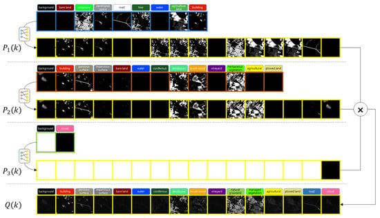
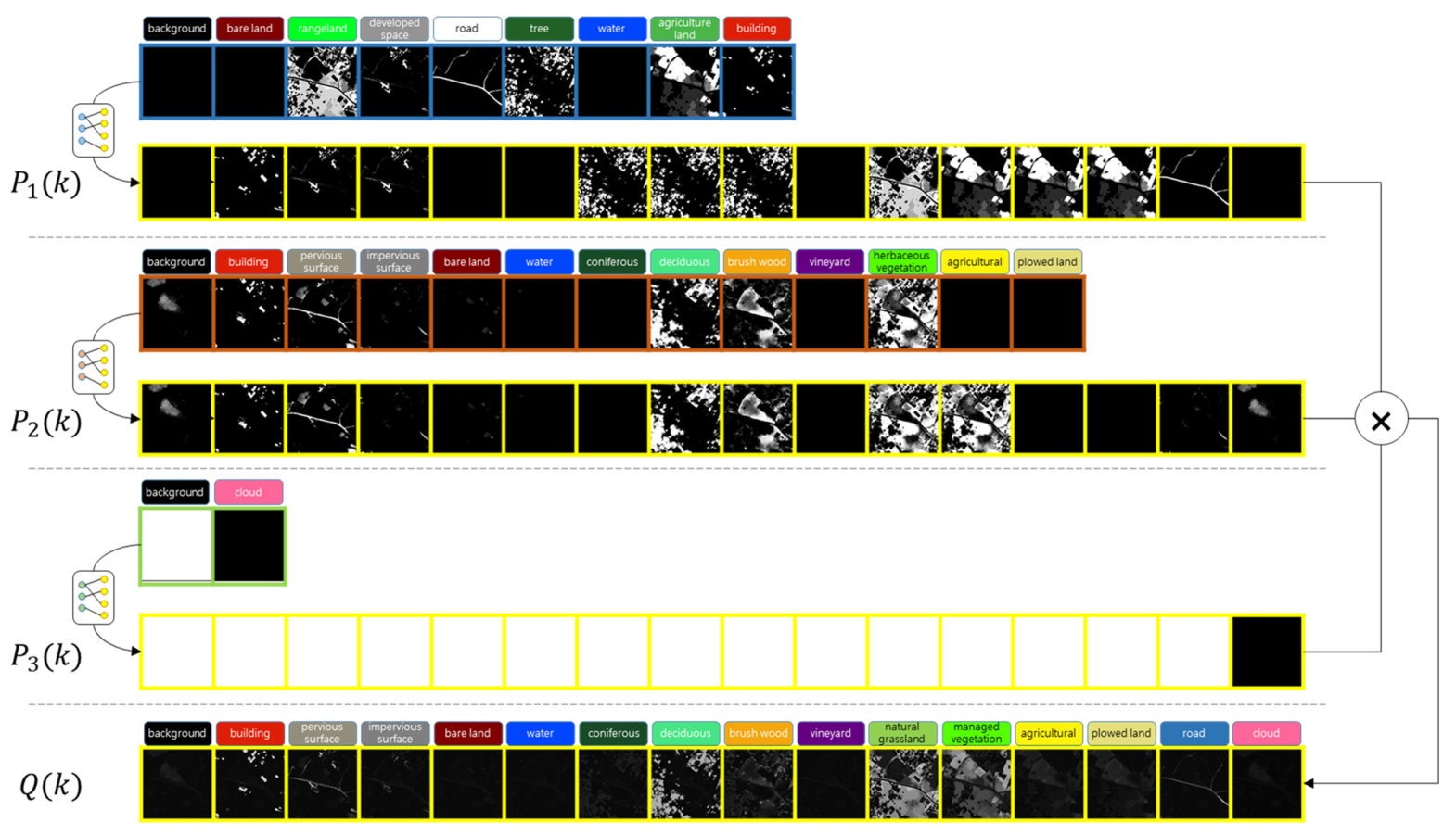
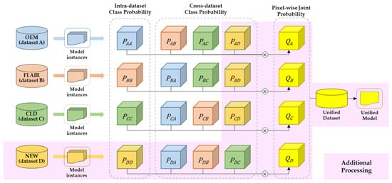
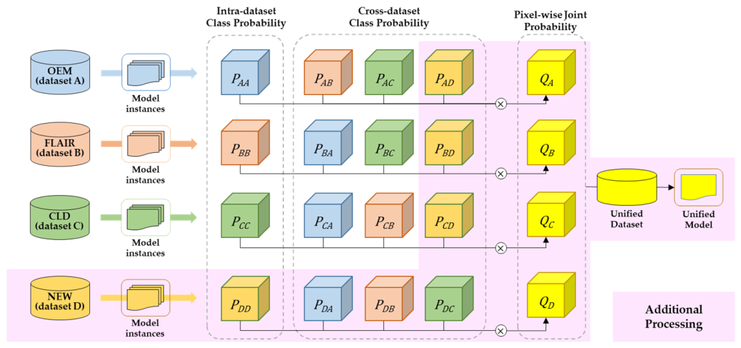
To evaluate the scalability of the proposed method, we consider integrating an additional dataset into our three-dataset fusion framework. If the new dataset’s classes match the existing unified label space, only the mapping between them needs to be established. Otherwise, the new classes are appended to the space, and overall dataset correspondences are updated accordingly. After training the MMIs on the new dataset, its intra- and cross-dataset pixel-wise class probabilities are computed, followed by the unification process shown in Figure 24.

Figure 24. Additional processing required to incorporate a new dataset into the proposed framework (shaded in light pink). Here, P denotes the pixel-wise class probability (first subscript: target dataset; second subscript: MMI training dataset), and Q represents the resulting pixel-wise joint probability.

Due to its systematic and flexible applicability, the proposed framework serves as a valuable tool for real-world applications where diverse and heterogeneous datasets coexist and continue to emerge. However, critical challenges remain, such as low-quality ground truth (GT) masks, highly disparate geographic environments, and divergent image sources. These factors can lead to a “dilution effect”—where increasing the number of datasets to be fused escalates data conflicts, thereby causing semantic confusion and suboptimal model training. While merging different land-cover types into a single class is straightforward and avoids contradictions, conflicts inevitably arise when identical land-cover types are categorized into distinct classes across datasets. The cloud class within the AIHub cloud dataset typified this issue, which we addressed by introducing an “ignorance factor.” Although this heuristic approach effectively resolves relatively simple cases, it has inherent limitations. Consequently, establishing optimal class mappings and systematic weight configurations remains a foundational and critical component for scaling the proposed framework.

To address this, we plan to semi-automate the design of the unified taxonomy and its associated mappings by analyzing cross-inference results generated by MMIs trained on individual datasets. Furthermore, we intend to deploy this framework on diverse legacy datasets constructed exclusively from KOMPSAT imagery [41,42,43,44]. Although these datasets feature disparate class compositions, they share identical sensor characteristics and imaging locations. Consequently, we anticipate more pronounced synergistic effects in dataset fusion compared to the baseline experiment in this study, where all variables—including imagery, geographical location, and class taxonomies—were entirely heterogeneous.

Regarding study scope, operational settings, and limitations, several methodological nuances warrant explicit discussion to provide guidance for future research. First, our comparison against competing paradigms—such as UDA, Geospatial Foundation Models, and manual fusion (Table 1)—is conceptual and operational rather than a direct head-to-head empirical benchmark; future studies could extend this work by conducting direct empirical benchmarking against fine-tuned foundation models and specific UDA frameworks. Second, in cross-dataset evaluations, models are assessed against consensus-harmonized masks from our MMI pipeline rather than independently re-annotated human ground truth, meaning reported metrics reflect alignment with a consensus-derived proxy ground truth; evaluating models on independently annotated cross-domain datasets provides a promising direction to further verify absolute generalizability. Third, while spatial resolutions across all datasets are standardized to a uniform 1.0 m per pixel (Section 2.1) to preserve structural detail relative to target masks, fine-grained object boundary delineation under extreme sub-meter spatial variations or unconstrained multi-sensor resolutions remains a practical challenge; testing edge-sensitive input adaptation techniques—such as adaptive patch reshaping [45]—offers a valuable trial for future boundary refinement.

6. Conclusions

This study introduced a consensus-based probabilistic fusion framework that reconciles heterogeneous satellite imagery datasets with disparate class taxonomies into a single, unified label space. By utilizing MMIs to compute pixel-wise joint class probabilities and incorporating dynamic uncertainty weights into parameter updates, the proposed data-centric approach effectively suppresses label noise and resolves structural ground-truth contradictions across domains.

Extensive benchmarking across six prominent segmentation architectures and contemporary backbone networks (including CNNs, Vision Transformers, and large-kernel ConvNets) demonstrated that the single unified model achieves substantial cross-dataset generalization improvements—averaging class-wise IoU gains of 17.5% in 2-fold cross-validation and 23.0% in holdout testing—while maintaining native intra-dataset accuracy. Furthermore, the framework successfully consolidates land-cover mapping with atmospheric cloud recognition into a single model without incurring active ensemble overhead or structural modifications during inference.

Future work will focus on semi-automating taxonomy mapping through cross-inference MMI analysis and mitigating data dilution effects when scaling the framework across large-scale legacy satellite archives.

References

- Ye, Z.; Yang, K.; Lin, Y.; Guo, S.; Sun, Y.; Chen, X.; Lai, R.; Zhang, H. A comparison between pixel-based deep learning and object-based image analysis (OBIA) for individual detection of cabbage plants based on UAV visible-light images. Comput. Electron. Agric. 2023, 209, 107822. [Google Scholar] [CrossRef] [Scilit]
- Zhang, X.; Han, L.; Han, L.; Zhu, L. How well do deep learning-based methods for land cover classification and object detection perform on high resolution remote sensing imagery? Remote Sens. 2020, 12, 417. [Google Scholar] [CrossRef] [Scilit]
- Fan, Z.; Zhan, T.; Gao, Z.; Li, R.; Liu, Y.; Zhang, L.; Jin, Z.; Xu, S. Land cover classification of resources survey remote sensing images based on segmentation model. IEEE Access 2022, 10, 56267–56281. [Google Scholar] [CrossRef] [Scilit]
- Müller, M.; Picone, D.; Demir, B.; Camps-Valls, G.; Dalla Mura, M.; Úlfarsson, M.Ö.; Benediktsson, J.A. Hybrid deep learning models for remote sensing image processing. Proc. IEEE 2025, 114, 396–416. [Google Scholar] [CrossRef] [Scilit]
- Southworth, J.; Smith, A.C.; Safaei, M.; Rahaman, M.; Alruzuq, A.; Tefera, B.B.; Muir, C.S.; Herrero, H.V. Machine learning versus deep learning in land system science: A decision-making framework for effective land classification. Front. Remote Sens. 2024, 5, 1374862. [Google Scholar] [CrossRef] [Scilit]
- Rao, S.S.; Rao, T.S.; Sowjanya, M.; Aruna, C.V. Deep learning and traditional methods for remote sensing image analysis. Discov. Imaging 2026, 3, 5. [Google Scholar] [CrossRef] [Scilit]
- Wang, J.; Zheng, Z.; Ma, A.; Lu, X.; Zhong, Y. LoveDA: A remote sensing land-cover dataset for domain adaptive semantic segmentation. In Proceedings of the Advances in Neural Information Processing Systems (NeurIPS), Virtual, 6–14 December 2021; Volume 34, pp. 1–15. [Google Scholar] [CrossRef] [Scilit]
- Chen, J.; Zhu, J.; Guo, Y.; Sun, G.; Zhang, Y.; Deng, M. Unsupervised domain adaptation for semantic segmentation of high-resolution remote sensing imagery driven by category-certainty attention. IEEE Trans. Geosci. Remote Sens. 2022, 60, 5616915. [Google Scholar] [CrossRef] [Scilit]
- Mendieta, M.; Han, B.; Shi, X.; Zhu, Y.; Chen, C. Towards geospatial foundation models via continual pretraining. In Proceedings of the 2023 IEEE/CVF International Conference on Computer Vision (ICCV), Paris, France, 2–6 October 2023; IEEE: Piscataway, NJ, USA, 2024; pp. 16760–16770. [Google Scholar] [CrossRef] [Scilit]
- Szwarcman, D.; Roy, S.; Fraccaro, P.; Gíslason, Þ.E.; Blumenstiel, B.; Ghosal, R.; de Oliveira, P.H.; de Sousa Almeida, J.L.; Sedona, R.; Kang, Y.; et al. Prithvi-EO-2.0: A versatile multi-temporal foundation model for earth observation applications. IEEE Trans. Geosci. Remote Sens. 2026, 64, 4400120. [Google Scholar] [CrossRef] [Scilit]
- Cong, Y.; Khanna, S.; Meng, C.; Liu, P.; Rozi, E.; He, Y.; Burke, M.; Lobell, D.; Ermon, S. SatMAE: Pre-training transformers for temporal and multi-spectral satellite imagery. In Proceedings of the Advances in Neural Information Processing Systems 35, New Orleans, LA, USA, 28 November–9 December 2022; Neural Information Processing Systems Foundation, Inc. (NeurIPS): South Lake Tahoe, NV, USA, 2022; pp. 197–211. [Google Scholar] [CrossRef] [Scilit]
- Xia, J.; Yokoya, N.; Adriano, B.; Broni-Bediako, C. OpenEarthMap: A benchmark dataset for global high-resolution land cover mapping. In Proceedings of the 2023 IEEE/CVF Winter Conference on Applications of Computer Vision (WACV), Waikoloa, HI, USA, 2–7 January 2023; IEEE: Piscataway, NJ, USA, 2023; pp. 6243–6253. [Google Scholar] [CrossRef] [Scilit]
- Sun, X.; Wang, P.; Yan, Z.; Xu, F.; Wang, R.; Diao, W.; Chen, J.; Li, J.; Feng, Y.; Xu, T.; et al. FAIR1M: A benchmark dataset for fine-grained object recognition in high-resolution remote sensing imagery. ISPRS J. Photogramm. Remote Sens. 2022, 184, 116–130. [Google Scholar] [CrossRef] [Scilit]
- He, K.; Zhang, X.; Ren, S.; Sun, J. Deep residual learning for image recognition. In Proceedings of the IEEE Conference on Computer Vision and Pattern Recognition (CVPR), Las Vegas, NV, USA, 27–30 June 2016; IEEE: Piscataway, NJ, USA, 2026; pp. 770–778. [Google Scholar] [CrossRef] [Scilit]
- Liu, Z.; Mao, H.; Wu, C.-Y.; Feichtenhofer, C.; Darrell, T.; Xie, S. A convnet for the 2020s. In Proceedings of the 2022 IEEE/CVF Conference on Computer Vision and Pattern Recognition (CVPR), New Orleans, LA, USA, 19–24 June 2022; IEEE: Piscataway, NJ, USA, 2022; pp. 11966–11976. [Google Scholar] [CrossRef] [Scilit]
- Wang, J.; Sun, K.; Cheng, T.; Jiang, B.; Deng, C.; Zhao, Y.; Liu, D.; Mu, Y.; Tan, M.; Wang, X.; et al. Deep high-resolution representation learning for visual recognition. IEEE Trans. Pattern Anal. Mach. Intell. 2020, 43, 3349–3364. [Google Scholar] [CrossRef] [Scilit] [PubMed]
- Liu, Z.; Lin, Y.; Cao, Y.; Hu, H.; Wei, Y.; Zhang, Z.; Lin, S.; Guo, B. Swin Transformer: Hierarchical vision transformer using shifted windows. In Proceedings of the 2021 IEEE/CVF International Conference on Computer Vision (ICCV), Montreal, QC, Canada, 11–17 October 2021; IEEE: Piscataway, NJ, USA, 2022; pp. 9992–10002. [Google Scholar] [CrossRef] [Scilit]
- Xie, E.; Wang, W.; Yu, Z.; Anandkumar, A.; Alvarez, J.M.; Luo, P. SegFormer: Simple and efficient design for semantic segmentation with transformers. In Proceedings of the Advances in Neural Information Processing Systems (NeurIPS), Virtual, 6–14 December 2021; Neural Information Processing Systems Foundation, Inc. (NeurIPS): South Lake Tahoe, NV, USA, 2021; Volume 34, pp. 12077–12090. [Google Scholar] [CrossRef] [Scilit]
- Xia, C.; Wang, X.; Lv, F.; Hao, X.; Shi, Y. ViT-CoMer: Vision Transformer with Convolutional Multi-scale Feature Interaction for Dense Predictions. In Proceedings of the 2024 IEEE/CVF Conference on Computer Vision and Pattern Recognition (CVPR), Seattle, WA, USA, 16–22 June 2024; IEEE: Piscataway, NJ, USA, 2024; pp. 5493–5502. [Google Scholar] [CrossRef] [Scilit]
- Ding, X.; Zhang, Y.; Ge, Y.; Zhao, S.; Song, L.; Yue, X.; Shan, Y. UniRepLKNet: A Universal Perception Large-Kernel ConvNet for Audio, Video, Point Cloud, Time-Series and Image Recognition. In Proceedings of the 2024 IEEE/CVF Conference on Computer Vision and Pattern Recognition (CVPR), Seattle, WA, USA, 16–22 June 2024; IEEE: Piscataway, NJ, USA, 2024; pp. 5513–5524. [Google Scholar] [CrossRef] [Scilit]
- Zhao, H.; Shi, J.; Qi, X.; Wang, X.; Jia, J. Pyramid scene parsing network. In Proceedings of the IEEE Conference on Computer Vision and Pattern Recognition (CVPR), Honolulu, HI, USA, 21–26 July 2017; IEEE: Piscataway, NJ, USA, 2017; pp. 2881–2890. [Google Scholar] [CrossRef] [Scilit]
- Chen, L.-C.; Zhu, Y.; Papandreou, G.; Schroff, F.; Adam, H. Encoder—Decoder with atrous separable convolution for semantic image segmentation. In Proceedings of the European Conference on Computer Vision (ECCV), Munich, Germany, 8–14 September 2018; Springer: Cham, Switzerland, 2018; pp. 833–851. [Google Scholar] [CrossRef] [Scilit]
- Xiao, T.; Liu, Y.; Zhou, B.; Jiang, Y.; Sun, J. Unified perceptual parsing for scene understanding. In Proceedings of the European Conference on Computer Vision (ECCV), Munich, Germany, 8–14 September 2018; Springer: Cham, Switzerland, 2018; pp. 432–448. [Google Scholar] [CrossRef] [Scilit]
- Yuan, Y.; Chen, X.; Wang, J. Segmentation Transformer: Object-contextual representations for semantic segmentation. In Proceedings of the European Conference on Computer Vision (ECCV), Glasgow, UK, 23–28 August 2020; Springer: Cham, Switzerland, 2020; pp. 173–190. [Google Scholar] [CrossRef] [Scilit]
- Zhang, W.; Pang, J.; Chen, K.; Loy, C.C. K-Net: Towards unified image segmentation. In Proceedings of the Advances in Neural Information Processing Systems (NeurIPS), Virtual, 6–14 December 2021; Neural Information Processing Systems Foundation, Inc. (NeurIPS): South Lake Tahoe, NV, USA, 2021; Volume 34, pp. 10326–10338. [Google Scholar] [CrossRef] [Scilit]
- Cheng, B.; Misra, I.; Schwing, A.G.; Kirillov, A.; Girdhar, R. Masked-attention mask transformer for universal image segmentation. In Proceedings of the 2022 IEEE/CVF Conference on Computer Vision and Pattern Recognition (CVPR), New Orleans, LA, USA, 19–24 June 2022; IEEE: Piscataway, NJ, USA, 2022; pp. 1280–1289. [Google Scholar] [CrossRef] [Scilit]
- Garioud, A.; Gonthier, N.; Landrieu, L.; De Wit, A.; Valette, M.; Poupée, M.; Giordano, S.; Wattrelos, B. FLAIR: A country-scale land cover semantic segmentation dataset from multi-source optical imagery. In Proceedings of the Advances in Neural Information Processing Systems, New Orleans, LA, USA, 10–16 December 2023; Neural Information Processing Systems Foundation, Inc. (NeurIPS): South Lake Tahoe, NV, USA, 2023; Volume 36, pp. 16456–16482. [Google Scholar] [CrossRef] [Scilit]
- Kim, B.; Oh, H. AI training dataset for cloud detection of KOMPSAT images. Geo Data 2020, 2, 56–62. [Google Scholar] [CrossRef] [Scilit]
- Sahr, K.; White, D.; Kimerling, A.J. Geodesic discrete global grid systems. Cartogr. Geogr. Inf. Sci. 2003, 30, 121–134. [Google Scholar] [CrossRef] [Scilit]
- Alomar, K.; Aysel, H.I.; Cai, X. Data augmentation in classification and segmentation: A survey and new strategies. J. Imaging 2023, 9, 46. [Google Scholar] [CrossRef] [Scilit] [PubMed]
- Zhang, M.; Arshad, H.; Abbas, M.; Jehanzeb, H.; Tahir, I.; Hassan, J.; Samad, Z.; Chunara, R. Quantifying greenspace with satellite images in Karachi, Pakistan, using a new data augmentation paradigm. ACM J. Comput. Sustain. Soc. 2025, 3, 1–23. [Google Scholar] [CrossRef] [Scilit]
- Lee, G.; Ju, J.; Kim, M.; Choe, J.; Chang, J.; Lee, K.-J. Adaptive remote sensing image enhancement for KOMPSAT imagery using reinforcement learning. Sensors 2026, 26, 1467. [Google Scholar] [CrossRef] [Scilit] [PubMed]
- Chang, J.Y.; Oh, K.-Y.; Lee, K.-J. Improving the universal performance of land cover semantic segmentation through training data refinement and multi-dataset fusion via redundant models. Remote Sens. 2025, 17, 2669. [Google Scholar] [CrossRef] [Scilit]
- Li, Y.; Zhong, X.; Liu, H.; Liao, M.; Lu, Y.; Liu, B. Urban built-up area extraction using triangle threshold algorithm and Naive Bayes classification model with multidata fusion. Sci. Rep. 2025, 15, 40175. [Google Scholar] [CrossRef] [Scilit] [PubMed]
- Dechesne, C.; Lassalle, P.; Lefèvre, S. Bayesian U-Net: Estimating uncertainty in semantic segmentation of earth observation images. Remote Sens. 2021, 13, 3836. [Google Scholar] [CrossRef] [Scilit]
- Bressan, P.O.; Junior, J.M.; Martins, J.A.C.; de Melo, M.J.; Gonçalves, D.N.; Freitas, D.M.; Ramos, A.P.M.; Furuya, M.T.G.; Osco, L.P.; J., de Andrade Silva; et al. Semantic segmentation with labeling uncertainty and class imbalance. Int. J. Appl. Earth Obs. Geoinf. 2022, 108, 102690. [Google Scholar] [CrossRef] [Scilit]
- Delibaşoğlu, İ. INCSA-UNET: Spatial attention inception UNET for aerial images segmentation. Comput. Inform. 2021, 40, 1244–1262. [Google Scholar] [CrossRef] [Scilit]
- de la Hidalga, A.N.; Rosin, P.L.; Sun, X.; Livermore, L.; Durrant, J.; Turner, J.; Dillen, M.; Musson, A.; Phillips, S.; Groom, Q.; et al. Cross-validation of a semantic segmentation network for natural history collection specimens. Mach. Vis. Appl. 2022, 33, 39. [Google Scholar] [CrossRef] [Scilit]
- Mohammadimanesh, F.; Salehi, B.; Mahdianpari, M.; Gill, E.; Molinier, M. A new fully convolutional neural network for semantic segmentation of polarimetric SAR imagery in complex land cover ecosystem. ISPRS J. Photogramm. Remote Sens. 2019, 151, 223–236. [Google Scholar] [CrossRef] [Scilit]
- Guo, M.-H.; Lu, C.-Z.; Hou, Q.; Liu, Z.; Cheng, M.-M.; Hu, S.-M. SegNeXt: Rethinking convolutional attention design for semantic segmentation. In Proceedings of the Advances in Neural Information Processing Systems 35, New Orleans, LA, USA, 28 November–9 December 2022; Neural Information Processing Systems Foundation, Inc. (NeurIPS): South Lake Tahoe, NV, USA, 2022; pp. 1140–1154. [Google Scholar] [CrossRef] [Scilit]
- Ye, C.; Ahn, Y. Hybrid object-based augmentation and histogram matching for cross-domain building segmentation in remote sensing. Appl. Sci. 2026, 16, 543. [Google Scholar] [CrossRef] [Scilit]
- Lee, C.; Lee, J.; Kim, T.; Lee, H.; Javed, A.; Chung, M.; Han, Y. MultiVeg: A very high-resolution benchmark for deep learning-based multi-class vegetation segmentation. Remote Sens. 2026, 18, 28. [Google Scholar] [CrossRef] [Scilit]
- Gong, S.-H.; Jung, H.-S.; Lee, M.-j.; Lee, K.-J.; Oh, K.-Y.; Chang, J.-Y. GeoAI dataset for rural hazardous facilities segmentation from KOMPSAT ortho mosaic imagery. Geo Data 2023, 5, 231–237. [Google Scholar] [CrossRef] [Scilit]
- Park, C.-W.; Jung, H.-S.; Lee, W.-J.; Lee, K.-J.; Oh, K.-Y.; Chang, J.-Y.; Lee, M.-j.; Han, G.-H.; Choi, I.-H. GeoAI dataset for industrial park and quarry classification from KOMPSAT-3/3A optical satellite imagery. Geo Data 2023, 5, 238–243. [Google Scholar] [CrossRef] [Scilit]
- Kosarevych, R.; Lutsyk, O.; Rusyn, B.; Pits, N.; Maksymyuk, T.; Volosin, M. Adaptive Patch Reshaping for Edge-Based Semantic Segmentation in Remote Sensing. IEEE Access 2026, 14, 38951–38964. [Google Scholar] [CrossRef] [Scilit]
Disclaimer/Publisher’s Note: The statements, opinions and data contained in all publications are solely those of the individual author(s) and contributor(s) and not of MDPI and/or the editor(s). MDPI and/or the editor(s) disclaim responsibility for any injury to people or property resulting from any ideas, methods, instructions or products referred to in the content. |
© 2026 by the authors. Licensee MDPI, Basel, Switzerland. This article is an open access article distributed under the terms and conditions of the Creative Commons Attribution (CC BY) license.