Background Suppression in EnMAP Methane Retrieval Maps with a Gated U-Net Denoiser

Highlights

What are the main findings?

• A multiplicatively gated U-Net suppresses positive background artifacts in EnMAP methane-enhancement maps while ensuring that the output cannot create or amplify positive signals absent from the raw matched-filter map.
• On held-out semi-synthetic data, the method reduced mean absolute background enhancement by approximately 80% and the false-positive rate by 72%, while retaining 70.4% of the injected plume-enhancement sum. Weak plume margins remained the main limitation.

What are the implications of the main findings?

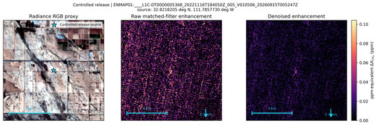
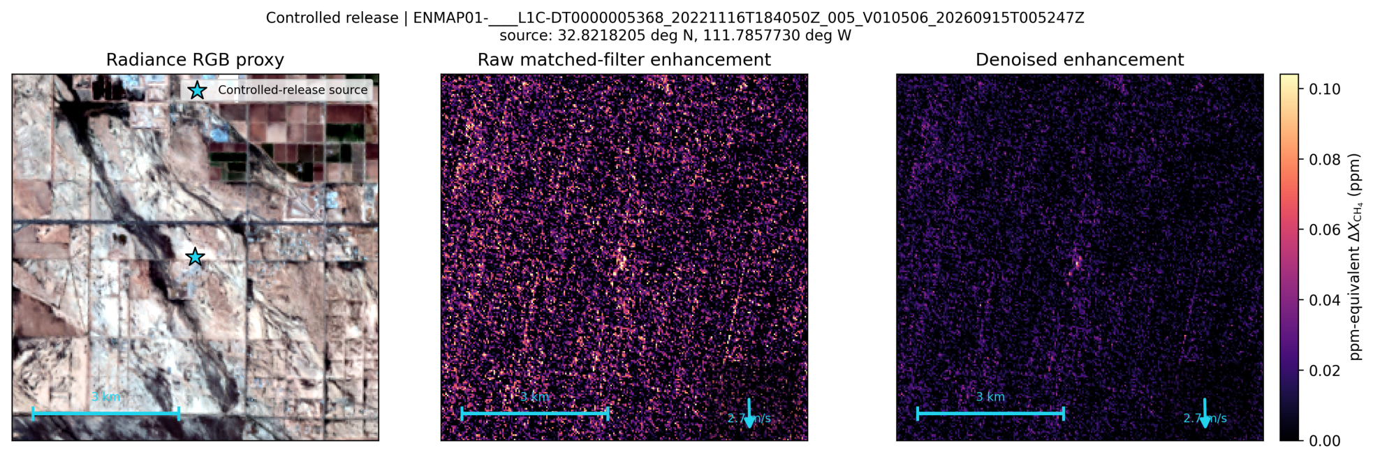
• Application to an independent EnMAP controlled-release acquisition retained a coherent enhancement at the documented source while suppressing distributed background texture, providing initial evidence of transfer to real observations.
• The retrieval-independent, non-amplifying design provides a practical framework for producing cleaner methane-enhancement maps alongside existing retrieval and plume-detection workflows, with broader real-plume evaluation as the next step toward operational use.

Abstract

High-resolution imaging spectrometers such as EnMAP can map methane point-source plumes, but retrieval maps often contain plume-like background artifacts associated with surface reflectance, snow, water, built surfaces, terrain-dependent optical paths, residual clouds and haze, and instrument effects. We present a gated U-Net denoiser that post-processes a single-band, ppm-equivalent methane enhancement map. The network predicts a pixel-wise retention factor that is multiplied by the positive part of the raw matched-filter map; it can therefore suppress or retain existing positive enhancement but cannot create or amplify it. Training combines semi-synthetic patches generated by injecting simulated methane absorption into real EnMAP L1C radiance, auxiliary EnMAP quality channels, and real-scene hard negatives. On a held-out set of 680 semi-synthetic patches, the selected gated U-Net reduced mean absolute background enhancement from 0.071 to 0.014 ppm and the false-positive rate at 0.05 ppm from 0.247 to 0.068, reductions of approximately 80% and 72%, respectively. Plume MAE decreased from 0.107 to 0.067 ppm, precision increased from 0.024 to 0.049, and average precision increased from 0.086 to 0.112. The denoised maps retained 70.4% of the injected plume-enhancement sum. Fixed-threshold recall decreased from 0.101 to 0.041 and FSS₇ from 0.079 to 0.064, showing that weak plume margins remain vulnerable to suppression. The results demonstrate substantial background reduction with improved ranking and retention of most plume enhancement. Application of the frozen model to an independent EnMAP controlled-release acquisition retained a plume-like enhancement at the documented source, although the absence of a registered physical plume mask precluded pixel-level or emission-rate validation. The method is therefore a promising constrained post-processing step, but broader independent real-plume validation is required before operational screening or quantitative emission-rate applications.

1. Introduction

Methane is a potent greenhouse gas, and rapid detection of point-source emissions is important for mitigation and emission verification [1,2,3]. High-spatial-resolution imaging spectrometers have demonstrated the ability to map methane plumes from airborne and spaceborne platforms. Matched-filter approaches are widely used for fast plume screening [4,5,6,7,8,9]. More physically explicit and nonlinear least-squares retrievals can improve quantitative accuracy, although they are often more computationally demanding for full-scene screening [9,10,11]. With the launch of EnMAP, high-spatial-resolution spaceborne hyperspectral observations now provide a new data source for greenhouse-gas studies [8,12,13].

Methane retrieval maps from imaging spectroscopy remain difficult to interpret in heterogeneous scenes. Retrieval artifacts can be caused by high-reflectance surfaces, water bodies, snow, concrete, roads, rooftops, terrain-induced path-length variations, residual clouds and haze, and instrument effects such as striping. These confusers are especially problematic for weaker emitters, such as landfills. In those cases, plume enhancements can be comparable to retrieval noise and to variability caused by surface and measurement conditions. Previous airborne and satellite studies have shown that noise, surface reflectance structure, albedo variability, and SWIR surface absorption features can produce spurious methane-like signals or degrade retrieval precision [4,6,14,15]. In practical plume-search workflows, such artifacts increase the amount of plume-like background signal that must be inspected and can make source localization more ambiguous.

Traditional post-processing strategies attempt to reduce this problem with background homogenization, spatial filtering, robust thresholding, or retrieval-specific corrections. Recent matched-filter developments, including log-domain filtering and background homogenization, explicitly target background variability in methane imagery [15,16,17,18]. However, they are often tied to a specific retrieval formulation or to a selected set of assumptions about the background. The goal of this work is to test whether a machine learning-based post-processing step can improve methane retrieval maps without replacing the retrieval itself.

Machine learning has already shown promise for methane plume segmentation and detection from hyperspectral or retrieval-derived inputs [19,20]. The present work addresses a narrower problem than direct plume segmentation: constrained background suppression in an existing methane retrieval product. The denoiser is designed to suppress background artifacts while retaining positive enhancement associated with plume structure. This is important because downstream tasks, such as plume identification, source localization, and emission-rate estimation, still benefit from a continuous retrieval map rather than only from a binary plume mask [6,21].

This paper presents a gated U-Net denoising pipeline for EnMAP methane retrieval maps. The main contributions are:

• A post-processing formulation that operates on single-band methane retrieval maps rather than on the full hyperspectral cube;
• A gated U-Net denoiser that predicts a retention factor and therefore can only reduce or preserve positive enhancement values already present in the raw matched-filter map;
• A training-data strategy combining semi-synthetic patches, auxiliary EnMAP quality channels, and real-scene hard negatives;
• An evaluation design that compares raw matched-filter maps, fixed classical reference filters, and gated U-Net denoising using complementary background-suppression and plume-retention metrics.

This paper is organized as follows. Section 2 describes the data, semi-synthetic augmentation, denoiser, reference methods, and evaluation. Section 3 presents the held-out test results and diagnostic analyses, followed by the discussion and conclusions in Section 4 and Section 5.

2. Materials and Methods

2.1. Data and Dataset Construction

This study uses EnMAP L1C hyperspectral radiance scenes. EnMAP provides contiguous VNIR–SWIR imaging spectroscopy at a ground sampling distance suitable for resolving strong methane point-source plumes [8,12,13,22]. The denoiser is trained and evaluated on methane retrieval maps derived from SWIR methane-sensitive bands rather than on the full hyperspectral cube.

Dense pixel-level labels for validated real methane plumes are scarce. We therefore create semi-synthetic patches by injecting simulated methane absorption into real EnMAP L1C radiance patches. The real radiance preserves surface, illumination, cloud, haze, snow, water, and instrument structure, while the injection supplies a known continuous enhancement target and binary plume mask. The final mixed index contains 4599 semi-synthetic $512\times 512$ patches from 115 EnMAP scenes and 220 real-scene patches from 16 scenes. The latter comprise 192 hard negatives and 28 weak positives. Table 1 summarizes the scene-level split. The complete test split contains 706 patches from 19 scenes; the 680 semi-synthetic test patches used for quantitative plume evaluation come from 17 of those scenes.

Table 1. Dataset accounting for the final mixed index. The split is performed at scene level. Semi-synthetic patches have dense injected plume fields and masks. Real hard-negative and weak-positive patches are used to reduce the synthetic-to-real domain gap; they are not used for the headline semi-synthetic plume-metric table.

Split	Semi-Synth.	Hard Neg.	Weak Pos.	Scenes	Total
Train	3239	132	22	92	3393
Validation	680	36	4	20	720
Test	680	24	2	19	706
All	4599	192	28	131	4819

The training split is used to fit network weights, and the validation split is used for checkpoint, architecture, loss, and inference operating-point selection. The held-out test split is used only for the final quantitative results, historical model comparison, and condition-stratified analysis. All splits are defined at the scene level so that no acquisition contributes patches to more than one split; this prevents leakage between training and evaluation data and avoids inflated performance estimates from spatially and hierarchically dependent observations [23]. Within a given scene, patches can still overlap spatially because they are sampled as local windows, so the reported evaluation should be interpreted as scene-stratified rather than as a fully independent patch-wise sample.

Real-scene hard negatives are patches with strong retrieval structure but no trusted plume after inspection of the retrieval map, RGB context, wind direction, and available scene information. They are assigned zero targets. These labels remain uncertain because the absence of a trusted plume does not prove the absence of weak or diffuse methane; this asymmetric label noise may contribute to suppression of weak plume margins. Weak positives are manually selected plume candidates for which the positive raw matched-filter signal is used as a noisy target. The three real-scene case studies shown in Section 3.4 contributed hard-negative and weak-positive training patches and therefore serve only as qualitative demonstrations. Independent real-scene validation requires retraining with those scenes, nearby tiles, and repeated acquisitions excluded from data mining.

2.2. Semi-Synthetic Patch Generation

The synthetic plume is defined in a source-centered, wind-aligned coordinate system rather than in the original map or image coordinates. The coordinate x denotes the downwind distance from the source measured parallel to the plume-transport direction, whereas y denotes the signed crosswind distance perpendicular to the plume centreline. The source is located at $(x,y)=(0,0)$. The original map coordinates are translated to the source position and rotated into the wind-aligned coordinate system. The plume model is evaluated only for $x>0$; the enhancement is set to zero for $x\le 0$.

The plume is represented by a Gaussian core using the Pasquill–Gifford/Turner rural dispersion widths [24,25,26]. The methane column-mass enhancement is given by

$$\Delta {\Omega }_{{\mathrm{CH}}_4}(x,y)=\left\{\begin{array}{cc}{\displaystyle \frac{Q}{2\pi u{\sigma }_y\left(x\right){\sigma }_z\left(x\right)}\exp \left[-\frac{y^2}{2{\sigma }_y^2\left(x\right)}\right]I_z\left(x\right)\exp \left[-\frac{x}{u{\tau }_{\mathrm{loss}}}\right],}\hfill & x>0,\hfill \\ 0,\hfill & x\le 0,\hfill \end{array}\right.$$

(1)

where Q is the methane emission rate, u is the plume-transport wind speed in the positive x-direction, and ${\sigma }_y\left(x\right)$ and ${\sigma }_z\left(x\right)$ are the stability-dependent crosswind and vertical dispersion widths, respectively. The vertical integration term is

$$I_z\left(x\right)={\int }_0^{z_{\mathrm{mix}}}\left[\exp \left(-{\displaystyle \frac{{(z-H)}^2}{2{\sigma }_z^2\left(x\right)}}\right)+\exp \left(-{\displaystyle \frac{{(z+H)}^2}{2{\sigma }_z^2\left(x\right)}}\right)\right]\mathrm{d}z,$$

(2)

where H is the effective release height, $z_{\mathrm{mix}}$ is the upper integration height, and the second Gaussian represents reflection at the ground. The factor involving ${\tau }_{\mathrm{loss}}$ represents an optional first-order reduction of methane during downwind transport. Column-mass enhancement is converted to dry-air mole-fraction enhancement using

$$\Delta X_{{\mathrm{CH}}_4}(x,y)=\Delta {\Omega }_{{\mathrm{CH}}_4}(x,y){\displaystyle \frac{M_{\mathrm{dry}\mathrm{air}}g}{M_{{\mathrm{CH}}_4}{p}_{\mathrm{dry},s}}},$$

(3)

where $M_{\mathrm{dry}\mathrm{air}}$ and $M_{{\mathrm{CH}}_4}$ are the molar masses of dry air and methane, g is gravitational acceleration, and $p_{\mathrm{dry},s}$ is the dry surface pressure. Bounded variations in the upper vertical integration height and aerodynamic roughness, together with plume-centreline meandering, source-rate variability, and along-plume texture, reduce the unrealistically smooth appearance of the idealized Gaussian plume labels. These empirical perturbations are intended to increase morphological variability and do not constitute an explicit or resolved model of atmospheric turbulence.

Injection is performed on calibrated and geocoded L1C radiance. The original patch therefore retains the scene-specific reflectance structure, geolocation footprint, residual atmosphere, striping, and instrument noise. No additional noise is added after injection, so signal-dependent noise changes caused by the added absorption are not simulated.

EnMAP metadata provide band centers and full widths at half maximum. The augmentation modifies SWIR bands 202–216 near 2.3μm. HITRAN methane lines are read through Py4CAtS and convolved to each band with a Gaussian spectral response. The default forward calculation uses the US Standard Atmosphere together with scene-mean elevation and viewing geometry; ERA5-derived atmospheres are used by the matched-filter retrieval where available. The optical-depth increment per 1 ppm column enhancement, ${\tau }_i^{1\mathrm{ppm}}$, is obtained by increasing methane uniformly within the sampled boundary layer and including solar and viewing path-length factors. The augmented radiance is

$$L_i^{\mathrm{aug}}(r,c)=L_i^{\mathrm{L}1\mathrm{C}}(r,c)\exp \left[-\Delta X_{{\mathrm{CH}}_4}(r,c){\tau }_i^{1\mathrm{ppm}}\right].$$

(4)

All other bands remain unchanged, and invalid pixels retain their nodata status.

The parameter choices used for the final augmentation run are summarized in Table 2.

Table 2. Main parameter choices used to generate the final semi-synthetic augmentation set. Values are implementation settings for the training data rather than retrieval priors.

Quantity	Setting Used in the Final Augmentation Run
Patch geometry	$512\times 512$ pixels, EnMAP L1C pixel size from the GeoTIFF transform, nominally 30 m
Patches per scene	40 patches per retained EnMAP scene
No-plume fraction	0.35; most no-plume examples are sampled preferentially from quality-flagged regions
Emission rate	Log-uniform between 100 and 50,000 kg h−1 per source
Wind speed	Sampled between 1 and 12 m s−1, with moderate winds favored
Wind direction	Uniform over 0–${360}^{\circ }$ for internal sources; outside-source winds are oriented so that plume signal can enter the patch, with random perturbation
Atmospheric stability	Pasquill classes A–F, mildly weighted toward neutral conditions
Mixing height	Stability-dependent default: approximately 1500, 1200, 900, 700, 450, and 250 m for A–F, with 20% lognormal variability
Roughness length	Log-uniform from ${10}^{-4}$ to 1 m, mapped to a bounded dispersion-width multiplier
Source placement	Mixed inside/outside placement; outside probability 0.3 and outside padding up to 256 pixels
Multiple sources	Probability 0.5 of more than one source, maximum four sources, with geometrically decaying probability for additional sources
Source variability	Fractional source-rate variability from 0 to 0.45 and correlation time from 20 to 600 s
Mask definition	Binary plume mask $P=1$ where $\Delta X_{{\mathrm{CH}}_4}\ge 0.005$ ppm
Quality filtering	Positive plume patches prefer quality-union fraction $\le 0.02$; positive masks must cover 0.0005–0.35 of valid pixels

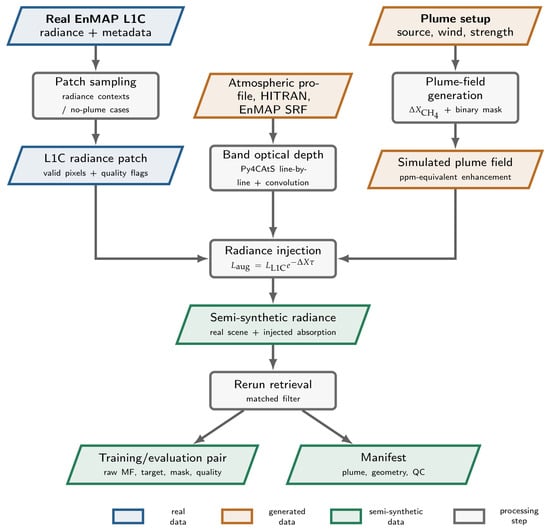
The patch-generation workflow is shown in Figure 1.

Figure 1. Semi-synthetic patch-generation workflow used to create the paired training and test patches. The injection is performed in radiance space before the matched-filter retrieval is rerun, while the target remains the known injected methane column enhancement.

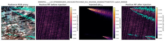
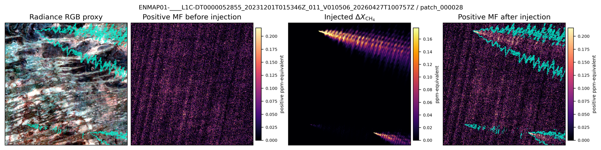
Figure 2 provides a representative example of the augmentation products.

Figure 2. Example semi-synthetic patch used to illustrate the augmentation products. The first panel shows the EnMAP L1C radiance context as an RGB proxy. The second panel shows the positive part of the matched-filter enhancement map obtained from the original, non-injected scene crop. The third panel shows the injected ppm-equivalent $\Delta X_{{\mathrm{CH}}_4}$ field, and the fourth panel shows the positive matched-filter enhancement map after radiance-space methane injection and rerunning the retrieval. The same zero-based color scale is used for the two matched-filter panels, so the positive retrieval response caused by the synthetic plume is directly visible.

The methane retrieval is rerun after injection. Its raw matched-filter enhancement map is the network input, while the known injected $\Delta X_{{\mathrm{CH}}_4}$ field remains the continuous target. The binary mask is used only for plume-weighted training and evaluation.

2.3. Retrieval Maps and Auxiliary Inputs

The method operates on a single-band retrieval map and is conceptually independent of the retrieval algorithm. The experiments reported here use a matched-filter product with ERA5 atmospheric correction; separate models would be required for retrievals with different scales or artifact distributions.

The raw matched-filter enhancement map, denoted M, is calibrated to the same ppm-equivalent column-average $\Delta X_{{\mathrm{CH}}_4}$ convention as the semi-synthetic target. It represents enhancement relative to a local background, not an absolute total-column $X_{{\mathrm{CH}}_4}$ field or a concentration-path-length quantity. The real-scene comparison figures display this enhancement directly, without adding a background column-average mole fraction. For one patch, $M\in {\mathbb{R}}^{H\times W}$, the target Y is the injected enhancement field, and P is its binary plume mask. For hard negatives, $Y=0$ and $P=0$.

Six binary EnMAP quality layers—cloud, cirrus, cloud shadow, haze, snow, and the EnMAP quality test-flags layer—are supplied as auxiliary channels rather than used as hard masks. They allow the network to associate retrieval artifacts with scene conditions without automatically discarding flagged pixels. Implementation-specific raster handling is documented in Appendix A.

The matched-filter map is robustly normalized per patch or inference tile

$$\tilde{M}={\displaystyle \frac{M-\mathrm{median}\left(M\right)}{1.4826\mathrm{MAD}\left(M\right)}},$$

(5)

where the statistics are computed over valid pixels. This scaling is less sensitive than mean–standard-deviation normalization to bright plume cores and isolated artifacts. If the MAD is unstable, the implementation falls back to the standard deviation or unit scale [27,28].

2.4. Gated U-Net Denoiser

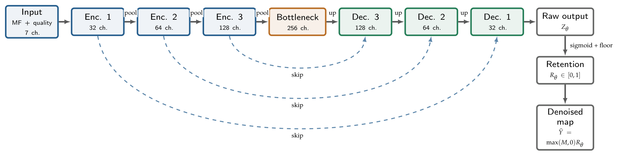
The denoiser is a compact U-Net with three encoder stages, a bottleneck, and three decoder stages [29]. Convolutional blocks use batch normalization and SiLU activations [30,31]. The model receives the normalized matched-filter map and six auxiliary quality channels and predicts a raw field $Z_{\theta }$. Unlike conventional residual denoising, which predicts an additive correction [32], the network is converted to a bounded multiplicative retention field.

The detailed architecture is listed in Table 3.

Table 3. Architecture of the gated denoising U-Net used in the final experiments.

Component	Configuration
Input channels	7: normalized matched-filter enhancement plus six binary auxiliary quality channels
Encoder widths	32, 64, 128 channels
Bottleneck width	256 channels
Decoder widths	128, 64, 32 channels with skip concatenation
Convolutional block	Two $3\times 3$ convolutions, padding 1, each followed by batch normalization and SiLU
Downsampling	$2\times 2$ max pooling
Upsampling	Bilinear interpolation followed by skip concatenation
Output layer	$1\times 1$ convolution to one raw output channel; sigmoid gate applied outside the U-Net
Trainable parameters	1,950,849

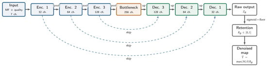
The corresponding data flow is shown in Figure 3.

Figure 3. Compact schematic of the gated U-Net denoiser. Each encoder and decoder stage consists of two $3\times 3$ convolution–batch-normalization–SiLU blocks. Skip connections concatenate encoder features with decoder features. The network predicts a raw field $Z_{\theta }$, which is converted to a bounded retention field $R_{\theta }$. The final denoised enhancement map is obtained by multiplying $R_{\theta }$ with the positive part of the raw matched-filter enhancement map.

The denoised enhancement map is

$$\widehat{Y}=\max (M,0)R_{\theta },0\le R_{\theta }\le 1,$$

(6)

with

$$R_{\theta }=R_{\min }+(1-R_{\min })\sigma \left(Z_{\theta }\right),$$

(7)

where $R_{\min }$ is the minimum retention, and $\sigma$ is the logistic sigmoid. The model can therefore suppress or retain positive input enhancement, but it cannot create positive enhancement where the input is non-positive or amplify it above the raw matched-filter value.

Training minimizes a plume-weighted L1 loss with an additional background penalty:

$$\mathcal{L}={\displaystyle \frac{{\sum }_i{w}_i|{\widehat{Y}}_i-Y_i|}{{\sum }_i{w}_i}}+{\lambda }_{\mathrm{bg}}{\displaystyle \frac{{\sum }_i(1-P_i)\left|{\widehat{Y}}_i\right|}{{\sum }_i(1-P_i)}}.$$

(8)

The plume weight and ${\lambda }_{\mathrm{bg}}$ control the balance between plume retention and background suppression. The reported values were selected through a targeted validation-set comparison; the present study does not claim that they are globally optimal.

2.5. Training and Operating-Point Selection

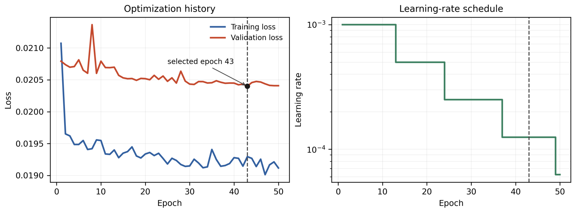
The selected model is trained from scratch on the mixed semi-synthetic and real-scene training split using AdamW [33]. Training uses 50 epochs, an initial learning rate of ${10}^{-3}$, weight decay ${10}^{-4}$, batch size 8, plume-pixel weight 18, background weight 1, and ${\lambda }_{\mathrm{bg}}=0.30$. The checkpoint with minimum validation loss (epoch 43) is retained. These loss weights were chosen through the targeted validation-set comparison conducted during model selection.

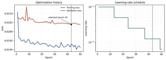
The training history and selected checkpoint are shown in Figure 4.

Figure 4. Training history of the selected gated U-Net. The selected checkpoint is marked at epoch 43, where the validation loss reaches its minimum. The left panel shows training and validation loss, while the right panel shows the ReduceLROnPlateau learning-rate schedule used for this training run. The history is used as a training diagnostic; all reported performance numbers are computed on the held-out semi-synthetic test split.

An inference-time signal-protection function can raise the minimum retention where the smoothed raw matched-filter map already contains coherent positive evidence. It is defined by a protected minimum retention $S_{\min }$, a robust z-score threshold $z_S$, transition width $w_S$, and smoothing radius $r_S$. These parameters alter only the gate-to-output conversion; they do not retrain the network. Their operating point is selected on the validation split in Section 3.2. Exact software parameter names and implementation settings are listed in Appendix A.

2.6. Reference Methods and Experimental Design

The semi-synthetic evaluation compares the raw matched-filter map, two fixed classical reference filters, and the gated U-Net denoiser. Real EnMAP scenes are used only as qualitative plausibility checks.

The homogenized reference removes a broad median background and then corrects row and column offsets:

$$M^{\left(0\right)}=M-\left[{\mathcal{M}}_{101}\left(M\right)-{\mathrm{median}}_{\Omega }\left({\mathcal{M}}_{101}\left(M\right)\right)\right],$$

(9)

Here, ${\mathcal{M}}_{101}\left(M\right)$ denotes a two-dimensional moving median of M evaluated with a $101\times 101$-pixel square window, using nearest-edge boundary handling, and ${\mathrm{median}}_{\Omega }$ denotes the median over the valid-pixel domain $\Omega$. This operation estimates and removes slowly varying background structure while preserving the global median level. It is followed by two row–column median-correction iterations. The local-percentile reference is

$$M_{\mathrm{lp}}=\max \left(M-{\mathcal{P}}_{30,101}\left(M\right),0\right),$$

(10)

where ${\mathcal{P}}_{30,101}$ is a moving 30th-percentile filter over a $101\times 101$ window. Both outputs are clipped to the positive-enhancement domain. These fixed configurations provide transparent, reproducible references but are not exhaustively optimized classical competitors. Boundary and invalid-pixel handling are documented in Appendix A.

2.7. Independent Controlled-Release Case Study

An independent EnMAP acquisition from the single-blind controlled-release campaign of Sherwin et al. [34] was used as an out-of-sample real-plume case study. The L1C acquisition was obtained on 16 November 2022 at 18:40:50 UTC over the release site at 32.8218205°N, 111.7857730°W. Sherwin et al. report that three of four participating teams detected the release in this EnMAP measurement, demonstrating both known plume presence and the difficulty of the observation. A subsequent study also used this acquisition for emission-rate experiments and published a manually bounded, rotated retrieval image [35].

The acquisition identifier was absent from the training, validation, test, hard-negative, weak-positive, and operating-point records used in this study. The selected checkpoint and operating point defined in Section 3.2 were fixed before this scene was processed; no model, retrieval, or inference parameter was tuned using this observation. The same matched-filter retrieval and gated U-Net inference chain used for the other real scenes was applied to the L1C radiance. The analysis uses a georeferenced $251\times 251$-pixel crop (approximately $7.5\times 7.5\mathrm{km}$) centered on the documented release coordinates. Raw and denoised panels use a common crop-derived color scale starting at zero. The arrow shows ERA5 1000 hPa wind used by the pipeline, rather than the campaign’s local anemometer measurement. Sherwin et al. report a five-minute on-site wind of $5.4[3.7,7.2]\mathrm{m}{\mathrm{s}}^{-1}$ for this EnMAP observation, whereas the ERA5 value used here is $2.7\mathrm{m}{\mathrm{s}}^{-1}$. This difference further precludes interpreting the case as an emission-rate validation.

This case establishes an independent known-source test, but not pixel-level ground truth. The campaign provides a metered release rate and published algorithm-dependent plume visualizations, not a registered physical plume mask for this L1C grid. Published masks differ among retrieval teams, and the bounding region used by Ouerghi et al. was manually drawn. We therefore do not calculate Dice, FSS, enhancement recovery, or emission rate for this scene, and use the case only to assess whether the frozen denoiser retains a spatially plausible enhancement at a documented active source.

2.8. Evaluation Metrics and Uncertainty

All metrics are computed on ppm-equivalent $\Delta X_{{\mathrm{CH}}_4}$ enhancement maps. Continuous metrics comprise plume MAE, mean and 95th-percentile absolute background enhancement, and the plume-enhancement sum ratio

$${\rho }_{\mathrm{sum}}={\displaystyle \frac{{\sum }_{i\in P}\max ({\widehat{Y}}_i,0)}{{\sum }_{i\in P}\max (Y_i,0)}}.$$

(11)

This unweighted image-domain ratio uses equal-area pixels and is not a plume-mass or emission-rate metric.

Threshold metrics use $\tau =0.05\mathrm{ppm}$ and include precision, recall, Dice, IoU, and

$$\mathrm{FPR}={\displaystyle \frac{\mathrm{FP}}{\mathrm{FP}+\mathrm{TN}}},$$

(12)

computed over valid background pixels [36,37,38,39]. Average precision (AP) is used as the ranking metric without linear interpolation or class weighting. Equal scores are grouped at each threshold; AP is the sum of precision multiplied by the corresponding recall increment. Thus, tied predictions do not receive an arbitrary ordering based on their pixel positions. The reported “best Dice” is a diagnostic threshold-scan upper envelope and is not an unbiased fixed-threshold test score.

FSS complements exact pixel overlap by comparing thresholded plume fractions within local neighborhoods [40]. ${\mathrm{FSS}}_r$ uses a radius r, so FSS₇ corresponds to a $15\times 15$ window (approximately $450\times 450$ m). Neighborhood means exclude invalid and outside-scene pixels. Object-level metrics are not reported because independent real-scene object annotations are unavailable.

Uncertainty is estimated at scene level. Patch metrics are averaged within each scene and summarized by the scene median and IQR. Confidence intervals for scene means are obtained from 5000 clustered-bootstrap replicates that resample scenes with replacement. Metrics requiring plume pixels are computed only for scenes containing injected plume signal; no-plume scenes contribute to background and false-positive metrics.

3. Results

3.1. Held-Out Semi-Synthetic Test Performance

The held-out semi-synthetic test split provides known continuous enhancement fields and plume masks, allowing all methods to be evaluated against the same reference. Table 4 reports results for 680 $512\times 512$ patches from 17 EnMAP scenes.

Table 4. Held-out semi-synthetic test split metrics for raw matched-filter maps, two classical post-processing baselines, and the selected gated U-Net denoiser. All methods are evaluated on the same 680 semi-synthetic test patches. MAE, background enhancement, and thresholds are reported in ppm-equivalent $\Delta X_{{\mathrm{CH}}_4}$. Lower values are better for MAE, background enhancement, and false-positive rate. Values closer to one are better for the plume-enhancement sum ratio defined in Equation (11). Higher values are better for precision, recall, AP, Dice, IoU, diagnostic best Dice, and FSS. Scene-level medians, interquartile ranges, and clustered-bootstrap confidence intervals for the headline metrics are reported in Table 5.

Method	N	MAEplume	BG abs.	BG p95	Sum Ratio	FPR	Prec.	Rec.	AP	Dice	IoU	Best Dice	FSS7
Raw MF	680	0.107	0.071	0.179	1.676	0.247	0.024	0.101	0.086	0.032	0.018	0.121	0.079
Homogenized	680	0.079	0.035	0.145	1.576	0.242	0.021	0.094	0.078	0.029	0.016	0.113	0.074
Local percentile	680	0.090	0.062	0.190	2.714	0.421	0.020	0.154	0.080	0.031	0.017	0.115	0.063
Gated U-Net	680	0.067	0.014	0.056	0.704	0.068	0.049	0.041	0.112	0.031	0.018	0.144	0.064

The raw matched-filter map has a plume-enhancement sum ratio of 1.676 and substantial positive background residuals. Homogenization reduces mean absolute background enhancement from 0.071 to 0.035 ppm but leaves FPR nearly unchanged, while local-percentile subtraction increases both FPR and the plume-enhancement sum ratio.

The selected gated U-Net provides the strongest background suppression. Relative to the raw matched-filter map, it reduces mean absolute background enhancement by approximately 80% (0.071 to 0.014 ppm), background p95 by 69% (0.179 to 0.056 ppm), and FPR by 72% (0.247 to 0.068). Plume MAE also decreases from 0.107 to 0.067 ppm. The plume-enhancement sum ratio moves closer to unity, from 1.676 to 0.704, although the bias changes from overestimation to underestimation.

Performance also improves for several detection-oriented metrics: precision increases from 0.024 to 0.049, average precision from 0.086 to 0.112, and the diagnostic best Dice from 0.121 to 0.144. These gains are accompanied by lower fixed-threshold recall (0.101 to 0.041) and FSS₇ (0.079 to 0.064), indicating that weak plume margins are still removed. The result is therefore a materially cleaner enhancement map with improved ranking and precision, but not yet a stand-alone thresholded plume detector.

Table 5 reports scene-level medians and IQRs for the same held-out split. Clustered-bootstrap confidence intervals are well separated for the two principal background metrics: BG p95 is 0.138–0.229 ppm for the raw matched filter and 0.044–0.072 ppm for the gated U-Net, while FPR is 0.211–0.285 and 0.038–0.105, respectively. The plume-enhancement sum-ratio intervals (1.262–2.124 for the raw map and 0.531–0.855 for the gated U-Net) confirm that the selected model reduces the raw overestimate but under-retains enhancement on unseen scenes. Confidence intervals overlap more strongly for average precision, Dice, and FSS₇; the strongest and most consistent evidence therefore concerns background suppression rather than exact plume-mask reconstruction.

Table 5. Scene-level distribution of selected metrics on the held-out semi-synthetic test split. Values are medians over scenes with interquartile ranges in parentheses. Within the 680-patch semi-synthetic evaluation set, background metrics use all 17 semi-synthetic test scenes. The plume-enhancement sum ratio and AP use the 12 semi-synthetic test scenes containing positive plume pixels.

Method	BG p95	FPR	Sum Ratio	AP	Dice	FSS7
Raw MF	0.146 (0.112–0.183)	0.231 (0.184–0.286)	1.339 (1.117–1.662)	0.094 (0.067–0.106)	0.039 (0.000–0.055)	0.090 (0.000–0.137)
Homogenized	0.115 (0.092–0.143)	0.230 (0.179–0.274)	1.311 (1.197–1.604)	0.082 (0.063–0.095)	0.037 (0.000–0.053)	0.086 (0.000–0.126)
Local percentile	0.152 (0.121–0.189)	0.409 (0.345–0.470)	2.226 (2.001–2.725)	0.086 (0.065–0.098)	0.039 (0.000–0.056)	0.066 (0.000–0.102)
Gated U-Net	0.045 (0.037–0.061)	0.035 (0.016–0.082)	0.569 (0.514–0.744)	0.126 (0.073–0.144)	0.025 (0.000–0.061)	0.049 (0.000–0.112)

3.2. Operating-Point Sweep

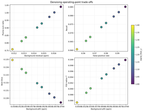
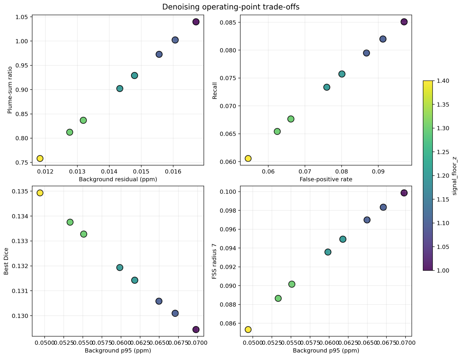
The gated formulation contains inference-time parameters that control how strongly positive raw matched-filter signal is retained. These parameters do not retrain the network; they only change the conversion from the predicted gate field to the final denoised enhancement map. To select a defensible operating point without using the held-out semi-synthetic test split, we evaluated a targeted validation sweep on all 680 semi-synthetic validation patches. The sweep used the checkpoint selected by the validation-set loss-weight comparison and varied the gate floor, signal floor, and signal-floor threshold over eight candidate settings that span conservative to high-retention behavior. The signal-floor width and smoothing radius were fixed to 0.9 and 10 pixels, respectively.

The sweep did not reveal a sharp optimum or tipping point. Instead, all metrics followed an almost monotonic trade-off between background suppression and plume preservation. Increasing the retention strength increased the plume-enhancement sum ratio, recall, and FSS, but also increased background residuals and the false-positive rate. This indicates that the selected inference parameters mainly control retention strength rather than changing the spatial ranking of plume-like pixels.

The validation trade-offs are shown in Figure 5.

Figure 5. Operating-point trade-offs for the gated U-Net on all 680 semi-synthetic validation patches. Each point corresponds to one inference-time parameter combination. The sweep shows a mostly monotonic trade-off between background suppression and plume preservation rather than a sharp optimum.

The selected validation operating point is $R_{\min }=0.20$, $S_{\min }=0.95$, $z_S=1.1$, $w_S=0.9$, and $r_S=10$ pixels. On the validation split, it yields a plume-enhancement sum ratio of 1.002, background p95 of 0.067 ppm, and FPR of 0.091. On the held-out test split, the sum ratio decreases to 0.704. This generalization gap shows that retention calibration is scene-dependent and reinforces the use of the locked test split for all performance claims. The representative settings from this validation sweep are reported in Table 6.

Table 6. Representative operating points from the 680-patch validation parameter sweep. The selected setting balances the plume-enhancement sum ratio and background suppression. The strict setting minimizes background residuals but underestimates the plume-enhancement sum, whereas the high-retention setting improves FSS but allows more background signal. The best Dice is the diagnostic threshold-scan upper envelope.

Setting	${\mathit{R}}_{\min }$	${\mathit{S}}_{\min }$	${\mathit{z}}_{\mathit{S}}$	BG p95	Sum Ratio	FPR	Best Dice	FSS7
Strict	0.15	0.85	1.4	0.049	0.758	0.054	0.135	0.085
Balanced	0.15	0.90	1.3	0.053	0.812	0.062	0.134	0.089
Selected	0.20	0.95	1.1	0.067	1.002	0.091	0.130	0.098
High-retention	0.20	0.95	1.0	0.070	1.040	0.097	0.129	0.100

3.3. Historical Model Comparison

Table 7 compares the raw and classical maps with historical direct-regression checkpoints and the selected gated model. The historical checkpoints differ in training data and loss weights, so this comparison does not isolate the causal effects of gating or hard-negative training. The table is therefore descriptive rather than a controlled one-factor-at-a-time ablation. The held-out test results were not used for checkpoint or operating-point selection.

Table 7. Historical model comparison on the 680-patch semi-synthetic test split. BG p95 is the 95th percentile of absolute background enhancement in ppm. FPR is the false-positive rate at $0.05\mathrm{ppm}$. Sum ratio is the plume-enhancement sum ratio defined in Equation (11). The best Dice column is the diagnostic threshold-scan upper envelope, not a validation-selected fixed threshold. The two distinct direct-regression checkpoints are included as historical neural baselines. Their near-zero background values are not interpreted as successful denoising, but as degenerate over-suppression solutions. The selected gated U-Net row is the final retrained model with the selected signal-floor inference setting. For this historical comparison, FSS₇ is averaged over the same 236 plume-containing test patches for every method, rather than the full 680-patch set used in the main comparison. This avoids method-dependent omission of blank patches where both observed and predicted neighborhood fractions are zero and FSS is undefined. Background performance is assessed separately by the background metrics and FPR.

Variant	BG p95	FPR	Sum Ratio	Best Dice (Diag.)	FSS7 (Plume Patches)	AP
Raw MF	0.179	0.247	1.68	0.121	0.227	0.086
Homogenized	0.145	0.242	1.58	0.113	0.214	0.078
Local percentile	0.190	0.421	2.71	0.115	0.183	0.080
Historical direct U-Net	$7.19\times {10}^{-5}$	$5.74\times {10}^{-5}$	0.15	0.205	0.121	0.186
Historical direct U-Net, mixed training	$3.08\times {10}^{-5}$	$3.50\times {10}^{-5}$	0.11	0.195	0.101	0.176
Selected gated U-Net	0.056	0.068	0.70	0.144	0.184	0.112

The early neural checkpoints collapse toward near-zero output: they achieve very low background metrics and relatively high threshold-optimized scores while retaining only 11–15% of the plume-enhancement sum. This illustrates why background or segmentation metrics alone are insufficient for model selection. The selected gated U-Net avoids this degenerate solution, retaining 70% of the plume-enhancement sum while keeping FPR at 0.068. Its lower FSS₇ relative to the raw matched filter indicates reduced retention of the spatially diffuse plume signal. On the common plume-containing subset, however, the selected model has a higher FSS₇ than either of the historical direct-regression models (0.184 versus 0.121 and 0.101). The historical models still have a higher AP and diagnostic best Dice, indicating that ranking and threshold-optimized overlap do not alone establish enhancement fidelity.

3.4. Real EnMAP Scene Examples

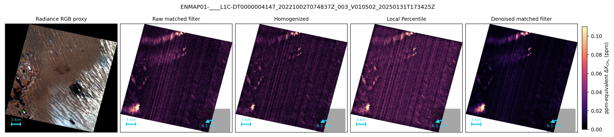
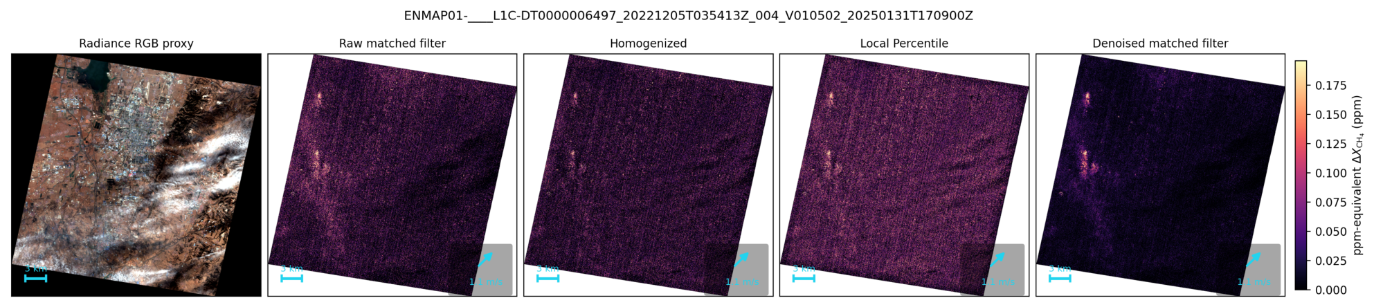
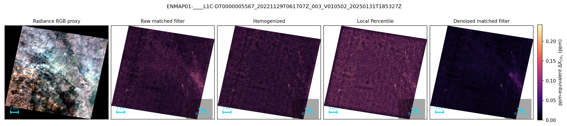
Three real EnMAP scenes illustrate behavior across oil-and-gas, coal, and landfill settings. The figures compare RGB context, the raw matched-filter enhancement map, the two classical references, and the denoised enhancement map. All retrieval panels within each figure share a color scale in ppm-equivalent $\Delta X_{{\mathrm{CH}}_4}$, starting at 0 ppm. The upper limit is the 99.5th percentile of the positive raw matched-filter map for that scene. Negative enhancements appear at the lower color limit, and values above the upper limit are saturated for display only; the underlying retrieval values and quantitative evaluations are unchanged. ERA5 1000 hPa wind arrows show the estimated transport direction, and scale bars use the 30 m EnMAP sampling distance. Because these scenes contributed training patches and lack independent plume annotations, they are qualitative plausibility examples rather than validation. They cannot establish that retained structures are methane or that removed structures are non-methane artifacts.

The three qualitative examples are shown in Figure 6, Figure 7, and Figure 8, respectively.

Figure 6. Real-scene denoising example over an oil-and-gas region in Turkmenistan, acquired by EnMAP on 2 October 2022 at 07:48:37 UTC (approximate scene center: 38.42°N, 54.16°E). The ERA5 1000 hPa wind used for the arrow is $6.1\mathrm{m}{\mathrm{s}}^{-1}$ toward ${250}^{\circ }$. The scene was selected because it combines suspected methane source activity with heterogeneous bright and dark background structures. The panels show the RGB context, raw matched-filter enhancement map, homogenized post-processing, local-percentile post-processing, and the denoised enhancement map. All retrieval panels share a color scale in ppm-equivalent $\Delta X_{{\mathrm{CH}}_4}$, starting at 0 ppm; no background mole fraction is added.

Figure 7. Real-scene denoising example over a coal-related methane scene in China, acquired by EnMAP on 5 December 2022 at 03:54:13 UTC (approximate scene center: 36.14°N, 113.10°E). The ERA5 1000 hPa wind used for the arrow is $1.1\mathrm{m}{\mathrm{s}}^{-1}$ toward ${45}^{\circ }$. This example illustrates behavior for a different industrial source type and background structure than the oil-and-gas case. All retrieval panels share a color scale in ppm-equivalent $\Delta X_{{\mathrm{CH}}_4}$, starting at 0 ppm; no background mole fraction is added.

Figure 8. Real-scene denoising example over a landfill-related methane scene in India, acquired by EnMAP on 29 November 2022 at 06:17:07 UTC (approximate scene center: 28.55°N, 77.21°E). The ERA5 1000 hPa wind used for the arrow is $0.9\mathrm{m}{\mathrm{s}}^{-1}$ toward ${119}^{\circ }$. Landfill plumes are often weaker and embedded in complex urban or peri-urban backgrounds, making this example relevant for illustrating the treatment of weaker plume-like structures and retrieval artifacts. All retrieval panels share a color scale in ppm-equivalent $\Delta X_{{\mathrm{CH}}_4}$, starting at 0 ppm; no background mole fraction is added.

3.5. Independent Controlled-Release Observation

Figure 9 applies the frozen model to the documented 16 November 2022 controlled release. The raw matched-filter crop contains widespread positive background texture together with a compact, spatially coherent enhancement at the release coordinate. The denoiser strongly attenuates the distributed background response while retaining the source-centered enhancement and visible downwind structure. The retained feature is spatially consistent with the narrow EnMAP plume visualizations published by Sherwin et al. and Ouerghi et al. [34,35]. This is a meaningful out-of-sample test because plume presence is established independently and the acquisition was not used for model development.

Figure 9. Independent EnMAP controlled-release case acquired on 16 November 2022 at 18:40:50 UTC near 32.8218205°N, 111.7857730°W. The cyan star in the RGB panel marks the documented release location. Raw and denoised panels show ppm-equivalent $\Delta X_{{\mathrm{CH}}_4}$ over the same approximately $7.5\times 7.5\mathrm{km}$ crop and share a crop-derived color scale that starts at 0 ppm. The arrow shows the ERA5 1000 hPa transport estimate used by the processing pipeline ($2.7\mathrm{m}{\mathrm{s}}^{-1}$, approximately southward), not the campaign’s five-minute on-site wind of $5.4[3.7,7.2]\mathrm{m}{\mathrm{s}}^{-1}$. The frozen gated U-Net suppresses widespread positive background texture while retaining a coherent enhancement at the independently documented active source. Because no registered physical plume mask is available, this figure supports real-plume retention qualitatively but does not constitute pixel-level recovery or emission-rate validation.

The comparison remains qualitative. Three of the four teams in the original single-blind experiment detected this EnMAP release, whereas one did not [34], illustrating that the observation is not trivial. However, neither the campaign publication nor the later analysis provides a georegistered physical plume mask suitable as pixel-level truth for our native L1C grid. Visual agreement with a published retrieval mask cannot measure enhancement recovery because that mask is itself method-dependent. Accordingly, we report neither segmentation scores nor an emission estimate for this scene.

3.6. Performance Stratified by Scene and Plume Conditions

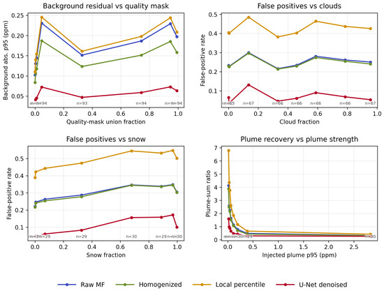
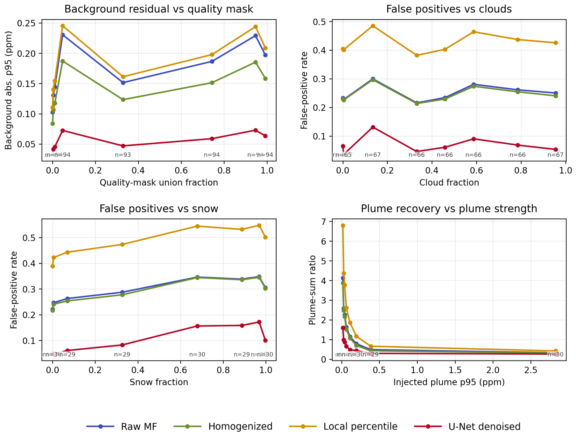
Performance is stratified by quality-mask fraction, cloud and snow fraction, and injected plume strength to assess whether the pooled results persist under difficult conditions. Figure 10 shows that the gated U-Net maintains lower background residuals and FPR than the raw and classical maps across the plotted quality bins. The plume-strength diagnostic also shows that the sum ratio is least stable for weak injections, where the denominator is small and retention estimates become sensitive to small absolute errors. Because some bins contain few positive patches, these curves are interpreted as sensitivity diagnostics; formal uncertainty is given by the scene-level bootstrap in Table 5.

Figure 10. Condition-stratified evaluation on the 680-patch semi-synthetic test split for raw matched-filter maps, classical post-processing baselines, and the selected gated U-Net. Lines show bin-wise means of patch metrics using up to eight predefined bins; bin counts are annotated in each panel. Bin intervals are derived from the held-out test values and reported in the generated condition-metric tables. The panels test whether performance changes with EnMAP quality-mask fraction, cloud fraction, snow fraction, and injected plume strength. The gated U-Net substantially reduces background residuals and above-threshold background signal in difficult quality-mask bins while generally keeping the plume-enhancement sum ratio closer to unity than the raw and classical products. Zero-fraction bins are kept separate from positive-contamination bins to distinguish clear scenes from cloud-, snow-, or quality-flagged cases. The plume-enhancement sum ratio becomes unstable for very weak injected plumes because the denominator in Equation (11) approaches zero; these bins are interpreted as qualitative sensitivity diagnostics rather than as quantitative plume-mass or emission-rate evidence.

4. Discussion

The held-out semi-synthetic results show that the gated U-Net can substantially clean EnMAP methane retrieval maps without replacing the physical retrieval. The model reduces mean absolute background enhancement by approximately 80% and FPR by 72%, while also lowering plume MAE and improving precision, average precision, and diagnostic best Dice. The denoised maps retain 70.4% of the injected plume-enhancement sum. Together, these results support the method as a useful constrained post-processing layer rather than merely a near-zero suppression solution.

The multiplicative gate is central to this interpretation. It prevents the network from creating or amplifying positive enhancement and leaves the raw retrieval available for quantitative analysis. Nevertheless, fixed-threshold recall and FSS₇ remain below the raw matched-filter values, showing that weak plume margins are still vulnerable. The largely monotonic validation sweep indicates that the current inference controls move along a background-versus-retention frontier rather than eliminating it. Broader loss-weight studies and additional weak positive examples are needed to improve that frontier.

The fixed classical references provide useful context. Homogenization removes broad structure but leaves the pixel-level FPR nearly unchanged, whereas local percentile subtraction can enhance both plume-like and non-plume maxima. The development-checkpoint comparison further shows that high ranking or threshold-optimized scores can coexist with severe under-retention of the continuous plume field. Evaluating background, ranking, overlap, and plume-enhancement retention together is therefore necessary for this task.

Semi-synthetic augmentation supplies dense, repeatable targets while preserving real EnMAP background structure, but it cannot represent every real plume morphology, atmospheric state, intermittency pattern, or signal-dependent sensor effect. Hard-negative labels may also contain weak methane, and the three sectoral real-scene examples are not independent because they contributed training patches. The controlled-release acquisition improves the evidence by providing an independent scene with externally established plume presence. The frozen model retained a coherent enhancement at the documented source while reducing surrounding background texture, and the result is qualitatively consistent with previously published retrievals of the same release. This observation shows that the behavior learned from the semi-synthetic and hard-negative data can transfer to at least one real plume.

One controlled release cannot characterize generalization across plume morphologies, source strengths, atmospheric stability regimes, or surface types. It also lacks a registered physical plume mask: the published outlines are products of other retrieval and masking methods rather than direct truth. Consequently, visual similarity cannot be converted into Dice, FSS, methane recovery, or emission-rate accuracy. Large-eddy-simulation plume families would provide a useful morphology-held-out stress test, but developing and validating such a simulator is beyond this proof-of-concept denoising study. Future work should combine diverse LES realizations with further controlled releases, repeat detections, aircraft observations, and independently defined plume annotations. Until then, the gated output is most appropriately used to support retrieval-map review and quality assurance, with the raw physical retrieval retained for quantitative interpretation.

The gating formulation is not restricted to CH₄ retrievals. In principle, it can be transferred to other trace-gas retrieval products that produce a positive-only enhancement map with plume-like background confounders, such as CO₂, NO₂ or NH₃ retrievals from imaging spectrometers. The same architecture would be well suited for plume screening, quality assurance, and anomaly suppression in other gas products, provided that the training data include a suitable enhancement target, physically meaningful quality or context inputs, and gas-specific nuisance patterns. We do not claim universal transfer without retraining and recalibration, because the spectral windows, background statistics, and retrieval sensitivities differ across gases and sensors. The method should therefore be viewed as a general constrained denoising framework for retrieval maps rather than a CH₄-only model.

5. Conclusions

This study demonstrates that a gated U-Net can provide substantial background suppression in EnMAP methane retrieval maps while enforcing a retrieval-constrained, non-amplifying output formulation. On the held-out 680-patch semi-synthetic test split, mean absolute background enhancement decreased from 0.071 to 0.014 ppm, background p95 from 0.179 to 0.056 ppm, and FPR from 0.247 to 0.068. Plume MAE, precision, average precision, and diagnostic best Dice also improved, and the denoised maps retained 70.4% of the injected plume-enhancement sum. Lower fixed-threshold recall and FSS₇ show that the retention of weak, spatially diffuse plume signals remains the main limitation. In an independent EnMAP controlled-release acquisition, the frozen model retained a coherent enhancement at the documented active source while suppressing distributed background texture. Because only one suitable controlled-release scene and no registered physical plume mask were available, this result is qualitative and does not validate pixel-level recovery or emission-rate accuracy. The selected model is therefore a promising background-suppression and quality-assurance layer, but broader independent real-plume validation is required before operational screening or quantitative emission-rate use.

Appendix A.1. Dataset and Software Settings

All selected patches have shape $512\times 512$, require corresponding quality rasters, and use auxiliary quality flags. In the implementation, these conditions are controlled by PATCH_SHAPE=512×512, REQUIRE_QUALITY=1, and USE_QUALITY_FLAGS=1. Scene-level split construction, real-patch mining, and network training use random seed 42. The reported evaluation was run with PyTorch 2.8.0. Py4CAtS 4.0.0 was used for the line-by-line calculations; https://atmos.eoc.dlr.de/tools/Py4CAtS/ (accessed on 18 February 2026). HITRAN data were accessed through HITRANonline at https://www.hitran.org/ (accessed on 19 February 2026).

Appendix A.2. Input Raster Handling

The six auxiliary channels are the EnMAP cloud, cirrus, cloud-shadow, haze, snow, and QL_QUALITY_TESTFLAGS layers. The last is an official quality layer and is unrelated to the train/validation/test split. Invalid normalized matched-filter pixels are set to zero and excluded through the valid-pixel mask. Quality rasters are binarized, invalid quality pixels are set to zero, and missing quality rasters are represented by zero-valued channels. Training augmentation is limited to random horizontal and vertical flips.

Appendix A.3. Network Implementation

Each encoder and decoder block contains two $3\times 3$ convolutions with stride 1 and padding 1, each followed by batch normalization and SiLU. Downsampling uses $2\times 2$ max pooling. Upsampling uses bilinear interpolation with align_corners=False, followed by skip-feature concatenation. The final $1\times 1$ convolution has no activation; the sigmoid is applied only in Equation (7). Default PyTorch parameter initialization is used. The seven-input, base-width-32 model has 1,950,849 trainable parameters.

Appendix A.4. Inference Parameter Names

The selected inference parameters and their software names are:

Parameter	Software Name	Selected Value
$R_{\min }$	GATE_FLOOR	0.20
$S_{\min }$	SIGNAL_FLOOR	0.95
$z_S$	SIGNAL_FLOOR_Z	1.1
$w_S$	SIGNAL_FLOOR_WIDTH	0.9
$r_S$	SIGNAL_FLOOR_SMOOTH_RADIUS	10 pixels

Appendix A.5. Classical Filter Implementation

For both classical references, invalid pixels are temporarily filled with the valid-scene median during filtering and restored afterward. Negative residuals are clipped to zero. The homogenized reference uses a $101\times 101$ median filter followed by two fixed row–column median-correction iterations and a final valid-median subtraction. The local-percentile reference uses a $101\times 101$ moving 30th-percentile filter. Both use nearest-neighbor boundary extension and no downsampling.

Appendix A.6. Supplementary Retrieval Details

For completeness, this section describes the classical matched filter that provides the input map to the denoiser. Let ${\mathbf{y}}_i\in {\mathbb{R}}^B$ be the radiance spectrum of spatial pixel i in the selected methane-sensitive SWIR bands. One scene-wide background model is estimated for each acquisition. Let ${\mathcal{I}}_b$ denote the scene pixels with a finite value in band b, and let N be the total number of spatial pixels:

$${\mu }_b={\displaystyle \frac{1}{|{\mathcal{I}}_b|}}\sum _{i\in {\mathcal{I}}_b}{y}_{ib},\mathbf{C}={\displaystyle \frac{1}{N-1}}{\displaystyle \sum _{i=1}^N}{\mathbf{z}}_i{\mathbf{z}}_i^{\mathsf{T}},z_{ib}=\left\{\begin{array}{cc}{y}_{ib}-{\mu }_b,\hfill & i\in {\mathcal{I}}_b,\hfill \\ 0,\hfill & i\notin {\mathcal{I}}_b.\hfill \end{array}\right.$$

(A1)

The “background window” is therefore the complete scene footprint, rather than a moving spatial neighborhood. Pixels missing any selected band remain invalid in the matched-filter output. The same $\mu$ and $\mathbf{C}$ are used for every valid output pixel in the scene.

The unitless methane optical-depth vector $\tau$ is calculated line by line from HITRAN spectroscopy. Absorption coefficients are integrated through atmospheric layers above the scene elevation along the downward solar and upward sensor paths, using the EnMAP solar and viewing zenith angles, and are convolved to the EnMAP band centers and full widths at half maximum. The radiance-space methane target is obtained by linearizing Beer–Lambert absorption around the scene mean, $\mathbf{s}=-\mu \odot \tau$, where ⊙ denotes element-wise multiplication. The coefficient for pixel i is then

$${\widehat{\alpha }}_i={\displaystyle \frac{{({\mathbf{y}}_i-\mu )}^{\mathsf{T}}{\mathbf{C}}^{+}\mathbf{s}}{{\mathbf{s}}^{\mathsf{T}}{\mathbf{C}}^{+}\mathbf{s}}},$$

(A2)

where ${\mathbf{C}}^{+}$ is the Moore–Penrose pseudo-inverse. The numerator measures the covariance-whitened similarity between the pixel anomaly and the methane target; the denominator normalizes the response by the target energy.

ERA5 provides the scene- and date-dependent pressure and temperature profile; the methane abundance is taken from the accompanying standard atmospheric gas profile. The combined atmosphere enters the calculation of $\tau$ and of the background column-average methane mole fraction $X_{\mathrm{bg}}$. ERA5 wind is used only for figure annotation and does not enter Equation (A2). Because the classical matched filter produces an anomaly coefficient centered near zero, its ppm-equivalent enhancement is calculated as

$$\Delta X_{{\mathrm{CH}}_4,i}\approx {\widehat{\alpha }}_i{X}_{\mathrm{bg}},$$

(A3)

which is the zero-background-coefficient case of $({\widehat{\alpha }}_i-{\alpha }_{\mathrm{bg}})X_{\mathrm{bg}}$. For semi-synthetic patches without scene-specific atmospheric metadata, a fixed $X_{\mathrm{bg}}=1.85$ ppm is used for this conversion. The resulting map is therefore a ppm-equivalent, background-referenced $\Delta X_{{\mathrm{CH}}_4}$ product under a linearized forward model, rather than an independent nonlinear retrieval of absolute $X_{{\mathrm{CH}}_4}$.

References

- United Nations Environment Programme; Climate and Clean Air Coalition. Global Methane Assessment: Benefits and Costs of Mitigating Methane Emissions. Technical Report, United Nations Environment Programme and Climate and Clean Air Coalition, Nairobi, 2021. Available online: https://www.unep.org/resources/report/global-methane-assessment-benefits-and-costs-mitigating-methane-emissions (accessed on 31 July 2026).
- Ocko, I.; Sun, T.; Shindell, D.; Oppenheimer, M.; Hristov, A.; Pacala, S.; Mauzerall, D.; Xu, Y.; Hamburg, S. Acting rapidly to deploy readily available methane mitigation measures by sector can immediately slow global warming. Environ. Res. Lett. 2021, 16, 054042. [Google Scholar] [CrossRef] [Scilit]
- Jacob, D.; Varon, D.; Cusworth, D.; Dennison, P.; Frankenberg, C.; Gautam, R.; Guanter, L.; Kelley, J.; McKeever, J.; Ott, L.; et al. Quantifying methane emissions from the global scale down to point sources using satellite observations of atmospheric methane. Atmos. Chem. Phys. 2022, 22, 9617–9646. [Google Scholar] [CrossRef] [Scilit]
- Thorpe, A.; Roberts, D.; Bradley, E.; Funk, C.; Dennison, P.; Leifer, I. High resolution mapping of methane emissions from marine and terrestrial sources using a Cluster-Tuned Matched Filter technique and imaging spectrometry. Remote Sens. Environ. 2013, 134, 305–318. [Google Scholar] [CrossRef] [Scilit]
- Thompson, D.; Thorpe, A.; Frankenberg, C.; Green, R.; Duren, R.; Guanter, L.; Hollstein, A.; Miller, C. Real-time remote detection and measurement for airborne imaging spectroscopy: A case study with methane. Atmos. Meas. Tech. 2015, 8, 4383–4395. [Google Scholar] [CrossRef] [Scilit]
- Cusworth, D.; Jacob, D.; Varon, D.; Chan Miller, C.; Liu, X.; Chance, K.; Thorpe, A.; Duren, R.; Miller, C.; Thompson, D.; et al. Potential of next-generation imaging spectrometers to detect and quantify methane point sources from space. Atmos. Meas. Tech. 2019, 12, 5655–5668. [Google Scholar] [CrossRef] [Scilit]
- Guanter, L.; Irakulis-Loitxate, I.; Gorroño, J.; Sánchez-García, E.; Cusworth, D.; Varon, D.; Cogliati, S.; Colombo, R. Mapping methane point emissions with the PRISMA spaceborne imaging spectrometer. Remote Sens. Environ. 2021, 265, 112671. [Google Scholar] [CrossRef] [Scilit]
- Roger, J.; Irakulis-Loitxate, I.; Valverde, A.; Gorroño, J.; Chabrillat, S.; Brell, M.; Guanter, L. High-Resolution Methane Mapping With the EnMAP Satellite Imaging Spectroscopy Mission. IEEE Trans. Geosci. Remote Sens. 2024, 62, 4102012. [Google Scholar] [CrossRef] [Scilit]
- Bettinelli, J.; Efremenko, D. Statistical retrieval pipeline for methane detection from hyperspectral satellite data. Light Eng. 2026. Epub ahead of printing. [Google Scholar]
- Thorpe, A.; Frankenberg, C.; Roberts, D. Retrieval techniques for airborne imaging of methane concentrations using high spatial and moderate spectral resolution: Application to AVIRIS. Atmos. Meas. Tech. 2014, 7, 491–506. [Google Scholar] [CrossRef] [Scilit]
- Gimeno García, S.; Schreier, F.; Lichtenberg, G.; Slijkhuis, S. Near infrared nadir retrieval of vertical column densities: Methodology and application to SCIAMACHY. Atmos. Meas. Tech. 2011, 4, 2633–2657. [Google Scholar] [CrossRef] [Scilit]
- Storch, T.; Honold, H.P.; Chabrillat, S.; Habermeyer, M.; Tucker, P.; Brell, M.; Ohndorf, A.; Wirth, K.; Betz, M.; Kuchler, M.; et al. The EnMAP imaging spectroscopy mission towards operations. Remote Sens. Environ. 2023, 294, 113632. [Google Scholar] [CrossRef] [Scilit]
- Chabrillat, S.; Foerster, S.; Segl, K.; Beamish, A.; Brell, M.; Asadzadeh, S.; Milewski, R.; Ward, K.; Brosinsky, A.; Koch, K.; et al. The EnMAP spaceborne imaging spectroscopy mission: Initial scientific results two years after launch. Remote Sens. Environ. 2024, 315, 114379. [Google Scholar] [CrossRef] [Scilit]
- Ayasse, A.; Thorpe, A.; Roberts, D.; Funk, C.; Dennison, P.; Frankenberg, C.; Steffke, A.; Aubrey, A. Evaluating the effects of surface properties on methane retrievals using a synthetic airborne visible/infrared imaging spectrometer next generation (AVIRIS-NG) image. Remote Sens. Environ. 2018, 215, 386–397. [Google Scholar] [CrossRef] [Scilit]
- Li, K.; Bai, K.; Fu, P.; Jiao, P.; Chen, H.; Huang, X.; Liu, C.; Chang, N.B. SSRMF: A sparse spectral reconstruction enhanced matched filter for improving point-source methane emission detection in complex terrain. ISPRS J. Photogramm. Remote Sens. 2025, 225, 238–256. [Google Scholar] [CrossRef] [Scilit]
- Foote, M.; Dennison, P.; Thorpe, A.; Thompson, D.; Jongaramrungruang, S.; Frankenberg, C.; Joshi, S. Fast and accurate retrieval of methane concentration from imaging spectrometer data using sparsity prior. IEEE Trans. Geosci. Remote Sens. 2020, 58, 6480–6492. [Google Scholar] [CrossRef] [Scilit]
- Pei, Z.; Han, G.; Mao, H.; Chen, C.; Shi, T.; Yang, K.; Ma, X.; Gong, W. Improving quantification of methane point source emissions from imaging spectroscopy. Remote Sens. Environ. 2023, 295, 113652. [Google Scholar] [CrossRef] [Scilit]
- Masin, F.; Maestri, T.; Martinazzo, M.; Pelliccia, G. Improved methane flux estimation from hyper-spectral imagery via log-domain matched filtering and background homogenization. Atmos. Environ. X 2026, 29, 100417. [Google Scholar] [CrossRef] [Scilit]
- Růžička, V.; Mateo-Garcia, G.; Gómez-Chova, L.; Vaughan, A.; Guanter, L.; Markham, A. Semantic segmentation of methane plumes with hyperspectral machine learning models. Sci. Rep. 2023, 13, 19999. [Google Scholar] [CrossRef] [Scilit] [PubMed]
- Rouet-Leduc, B.; Hulbert, C. Automatic detection of methane emissions in multispectral satellite imagery using a vision transformer. Nat. Commun. 2024, 15, 3801. [Google Scholar] [CrossRef] [Scilit] [PubMed]
- Varon, D.; Jacob, D.; McKeever, J.; Jervis, D.; Durak, B.; Xia, Y.; Huang, Y. Quantifying methane point sources from fine-scale satellite observations of atmospheric methane plumes. Atmos. Meas. Tech. 2018, 11, 5673–5686. [Google Scholar] [CrossRef] [Scilit]
- Guanter, L.; Kaufmann, H.; Segl, K.; Foerster, S.; Rogaß, C.; Chabrillat, S.; Küster, T.; Hollstein, A.; Rossner, G.; Chlebek, C.; et al. The EnMAP Spaceborne Imaging Spectroscopy Mission for Earth Observation. Remote Sens. 2015, 7, 8830–8857. [Google Scholar] [CrossRef] [Scilit]
- Roberts, D.; Bahn, V.; Ciuti, S.; Boyce, M.; Elith, J.; Guillera-Arroita, G.; Hauenstein, S.; Lahoz-Monfort, J.; Schröder, B.; Thuiller, W.; et al. Cross-validation strategies for data with temporal, spatial, hierarchical, or phylogenetic structure. Ecography 2017, 40, 913–929. [Google Scholar] [CrossRef] [Scilit]
- Pasquill, F. The estimation of the dispersion of windborne material. Meteorol. Mag. 1961, 90, 33–49. [Google Scholar]
- Gifford, F. Use of routine meteorological observations for estimating atmospheric dispersion. Nucl. Saf. 1961, 2, 47–51. Available online: https://archive.org/details/sim_nuclear-safety_1961-06_2_4 (accessed on 20 September 2026).
- Turner, D. Workbook of Atmospheric Dispersion Estimates; AP-26; U.S. Environmental Protection Agency, Office of Air Programs: Research Triangle Park, NC, USA, 1970.
- Leys, C.; Ley, C.; Klein, O.; Bernard, P.; Licata, L. Detecting outliers: Do not use standard deviation around the mean, use absolute deviation around the median. J. Exp. Soc. Psychol. 2013, 49, 764–766. [Google Scholar] [CrossRef] [Scilit]
- NIST/SEMATECH. NIST/SEMATECH e-Handbook of Statistical Methods: Measures of Scale. Available online: https://www.itl.nist.gov/div898/handbook/eda/section3/eda356.htm (accessed on 22 July 2026).
- Ronneberger, O.; Fischer, P.; Brox, T. U-Net: Convolutional Networks for Biomedical Image Segmentation. In Proceedings of the Medical Image Computing and Computer-Assisted Intervention—MICCAI 2015; Springer: Cham, Switzerland, 2015; pp. 234–241. [Google Scholar] [CrossRef] [Scilit]
- Ioffe, S.; Szegedy, C. Batch Normalization: Accelerating Deep Network Training by Reducing Internal Covariate Shift. In Proceedings of the 32nd International Conference on Machine Learning, Lille, France, 6–11 July 2015; Volume 37, pp. 448–456. [Google Scholar]
- Ramachandran, P.; Zoph, B.; Le, Q. Searching for Activation Functions. In Proceedings of the International Conference on Learning Representations Workshop, Vancouver, BC, Canada, 30 April–3 May 2018. [Google Scholar]
- Zhang, K.; Zuo, W.; Chen, Y.; Meng, D.; Zhang, L. Beyond a Gaussian Denoiser: Residual Learning of Deep CNN for Image Denoising. IEEE Trans. Image Process. 2017, 26, 3142–3155. [Google Scholar] [CrossRef] [Scilit] [PubMed]
- Loshchilov, I.; Hutter, F. Decoupled Weight Decay Regularization. In Proceedings of the International Conference on Learning Representations, New Orleans, LA, USA, 6–9 May 2019. [Google Scholar]
- Sherwin, E.D.; El Abbadi, S.H.; Burdeau, P.M.; Zhang, Z.; Chen, Z.; Rutherford, J.S.; Chen, Y.; Brandt, A.R. Single-blind test of nine methane-sensing satellite systems from three continents. Atmos. Meas. Tech. 2024, 17, 765–782. [Google Scholar] [CrossRef] [Scilit]
- Ouerghi, E.; Ehret, T.; Facciolo, G.; Meinhardt, E.; Marion, R.; Morel, J.M. Tightening up methane plume source rate estimation in EnMAP and PRISMA images. Atmos. Meas. Tech. 2025, 18, 4611–4629. [Google Scholar] [CrossRef] [Scilit]
- Jolliffe, I. The Dice coefficient: A neglected verification performance measure for deterministic forecasts of binary events. Meteorol. Appl. 2016, 23, 89–90. [Google Scholar] [CrossRef] [Scilit]
- Taha, A.; Hanbury, A. Metrics for evaluating 3D medical image segmentation: Analysis, selection, and tool. BMC Med. Imaging 2015, 15, 29. [Google Scholar] [CrossRef] [Scilit] [PubMed]
- Davis, J.; Goadrich, M. The Relationship Between Precision-Recall and ROC Curves. In Proceedings of the 23rd International Conference on Machine Learning, Pittsburgh, PA, USA, 25–29 June 2006; pp. 233–240. [Google Scholar] [CrossRef] [Scilit]
- Fawcett, T. An introduction to ROC analysis. Pattern Recognit. Lett. 2006, 27, 861–874. [Google Scholar] [CrossRef] [Scilit]
- Roberts, N.; Lean, H. Scale-Selective Verification of Rainfall Accumulations from High-Resolution Forecasts of Convective Events. Mon. Weather Rev. 2008, 136, 78–97. [Google Scholar] [CrossRef] [Scilit]
Disclaimer/Publisher’s Note: The statements, opinions and data contained in all publications are solely those of the individual author(s) and contributor(s) and not of MDPI and/or the editor(s). MDPI and/or the editor(s) disclaim responsibility for any injury to people or property resulting from any ideas, methods, instructions or products referred to in the content. |
© 2026 by the authors. Licensee MDPI, Basel, Switzerland. This article is an open access article distributed under the terms and conditions of the Creative Commons Attribution (CC BY) license.