Supercooled Water Cloud Identification by Himawari-8, Its Validation by CALIPSO and Application to the Northeast China Cold Vortex

Highlights

What are the main findings?

• A two-step supercooled water cloud (SWC) identification method using Himawari-8 is presented, and validation against CALIPSO shows that the proposed SWC identification method has a high hit rate of 89.3%.
• Supercooled water clouds (SWCs) exhibit significant spatial heterogeneity and distinct diurnal and vertical evolution in late spring 2021 during Northeast China Cold Vortex (NCCV) weather events.

What are the implications of the main findings?

• This study provides a validated, two-step Himawari-8 SWC identification method with a high hit rate, which satisfies the requirements for operational cold-cloud seeding, enhances precipitation efficiency, and facilitates the integration of satellite remote sensing into weather modification practices.
• The significant presence of SWCs in NCCV offers improved observational constraints for cloud microphysical studies and cold-vortex-related weather forecasting.

Abstract

Accurate identification of supercooled water cloud (SWC) is critical for precipitation enhancement, reducing the risk of aircraft icing, and advancing our understanding of Earth’s radiative energy budget. However, SWC detection is frequently missed in the current official satellite products. To fill this observational gap and to investigate the potential use of the Himawari-8 satellite observation in the Northeast China Cold Vortex (NCCV) research, this study introduces an efficient algorithm to detect SWC from the Advanced Himawari Imager (AHI), which first uses a random forest (RF) model to classify the cloud into nine cloud types—high ice cloud, high water cloud, high mixed cloud, middle ice cloud, middle water cloud, middle mixed cloud, low water cloud, low ice cloud and low mixed cloud. Then, with the level 2 products, i.e., cloud optical thickness (COT), cloud effective radius (CER) and cloud-top temperature (CTT), the SWCs will further be identified from the water clouds and the mixed clouds. Validated by the dataset from AHI and labels derived from the Cloud-Aerosol LiDAR and Infrared Pathfinder Satellite Observation (CALIPSO) vertical feature mask (VFM), our algorithm can correctly detect 89.3% of SWC pixels in the dataset, which satisfies the requirements for operational cold-cloud seeding, enhances precipitation efficiency, and facilitates the integration of satellite remote sensing into weather modification practices. Based on AHI data in late spring 2021 during the NCCV weather event, SWCs exhibit significant spatial heterogeneity and distinct diurnal vertical evolution. These clouds occur most frequently in the southwest quadrant and evolve progressively from mid- and low-level layers to the high-level layer.

1. Introduction

Clouds constitute one of the most significant sources of uncertainty in present-day climate modeling and projections of global warming [1,2]. A major contributor to this uncertainty lies in the representation of cloud microphysical properties, among which the cloud thermodynamic phase plays a pivotal role. The phase state of clouds—whether composed of ice, liquid, or a mixture of both—critically governs cloud-radiation interactions by modulating the cloud albedo, emissivity, and lifetime [3,4]. Consequently, accurate phase discrimination directly impacts the simulation of Earth’s energy budget and the magnitude of climate sensitivity in general circulation models (GCMs). Beyond radiative effects, knowledge of cloud phase is also fundamental to understanding cloud and precipitation development processes, such as the Wegener–Bergeron–Findeisen (WBF) process, wherein ice crystals grow at the expense of supercooled liquid droplets in mixed-phase environments [5]. Based on the thermodynamic phase of hydrometeors, clouds are conventionally classified into three categories: ice clouds, liquid water clouds, and mixed-phase clouds [6]. Notably, clouds with liquid cloud droplets below 0 °C are defined as supercooled water clouds (SWCs) [7]. Under this definition, both sub-zero liquid water clouds and mixed-phase clouds fall within the broader SWC category. Given that SWCs serve as the primary target for precipitation enhancement operations—such as glaciogenic cloud seeding—and are a critical consideration in aircraft icing certification and aviation safety [8,9], their accurate identification carries implications that extend beyond climate and weather research. Precise SWC detection not only reduces uncertainties in cloud radiative feedback estimates but also supports operational meteorology and meteorological engineering applications.

The Northeast China cold vortex (NCCV) is a large-scale upper-level synoptic system characterized by a quasi-stationary, cold-core low-pressure circulation that develops over or in the vicinity of northeastern China [10]. As a deep and dynamically active system, the NCCV is capable of persisting for 3–4 days or even longer, often maintaining its structure while propagating slowly across the region. Although it can occur throughout the year, its frequency and intensity peak during the late spring to early summer transition period, when the large-scale circulation undergoes significant seasonal adjustment [11]. Northeast China serves as the country’s most important commodity grain production base, contributing a substantial proportion of national cereal output. Consequently, grain yield in this region exerts a direct and profound influence on national food security as well as on broader socioeconomic and ecological stability [12,13]. Within this climatic context, the NCCV frequently acts as a dominant precipitation-producing system, generating widespread stratiform cloud decks that are rich in supercooled liquid water. As such, artificial precipitation enhancement operations conducted under NCCV conditions have long been regarded as a critical technological measure to alleviate drought, stabilize agricultural production, and safeguard food security in Northeast China [14]. Given the central role of supercooled water in both the microphysical evolution of cold vortex clouds and the efficacy of glaciogenic seeding, the accurate identification of supercooled water clouds (SWCs) within NCCV systems is not only vital for optimizing precipitation enhancement strategies but also holds considerable significance for national food security planning and meteorological disaster mitigation.

Knowledge of supercooled water clouds (SWCs) within the Northeast China cold vortex (NCCV) system can be acquired through two primary approaches: in situ airborne measurements and remote sensing observations [8]. In situ airborne probes provide direct, high-resolution microphysical measurements of cloud particle size distributions, phase states, and liquid water content, offering a level of accuracy that is currently unmatched by other techniques. However, airborne campaigns are inherently limited by high operational costs, flight restrictions, and safety concerns under severe weather conditions, making it difficult to sustain long-term, continuous monitoring of cloud system evolution across the entire lifecycle of an NCCV event. In contrast, remote sensing platforms, particularly spaceborne satellite sensors, are capable of providing continuous, long-duration, and large-scale monitoring of cloud properties. Satellites offer the unique advantage of consistent temporal coverage and spatial extent, enabling the observation of SWC distribution and temporal variability across the vast geographic area influenced by the cold vortex. Furthermore, advances in passive and active satellite remote sensing—such as multi-spectral imagers and cloud radar—have significantly improved the ability to retrieve cloud thermodynamic phase and estimate supercooled liquid water paths. Consequently, utilizing satellite data to observe and characterize supercooled cloud water within NCCV events represents a highly effective strategy. This approach not only complements the limitations of airborne measurements but also provides critical, operationally relevant data for weather monitoring, nowcasting, and the planning and evaluation of weather modification activities, such as precipitation enhancement operations.

The Himawari-8 (H-8) geostationary satellite was launched by the Japan Meteorological Agency and became operational in July 2015 [15]. It provides a significant increase in the spatial (2–5 km) and temporal (10 min) resolution of imagery. The satellite has an Advanced Himawari Imager (AHI) in it, which allows for aerosol and cloud retrievals. Owing to the nearly uninterrupted sampling capability of Himawari-8, its datasets are well-suited to analyze how the SWCs in NCCV weather systems change spatially and temporally as they develop across its observation coverage. Although official cloud phase (CPH) outputs—including ice, liquid water, and mixed-phase hydrometeors—are publicly available, they lack explicit classification of SWCs. Wang et al. [16] utilized H-8’s Level 2 cloud products—including cloud phase (CPH), cloud optical thickness (COT), cloud effective radius (CER), and cloud-top temperature (CTT)—to identify SWCs by applying empirically derived thresholds. Although this method yielded a high detection rate, it also incurred a substantial false alarm rate, partly attributed to inherent limitations in the initial cloud products. Fu et al. [17] leveraged thermal infrared (TIR) channels of H-8 and a machine learning technique to develop an all-day SWC identification model. But the model’s accuracy rate is limited.

In this study, four L1-level infrared band products from AHI (with a spatial resolution of 2 km) were used as inputs to a random forest-based cloud phase classification model, which can classify the cloud phase into water cloud, ice cloud and “mixed-phase” cloud. Then, with the AHI Level 2 products—cloud optical thickness (COT), cloud effective radius (CER), cloud-top temperature (CTT)—the water cloud and the mixed-phase cloud will be further identified as SWCs. Based on the cloud phase information from Cloud-Aerosol Lidar and Infrared Pathfinder Satellite Observations (CALIPSO) Level 2 products [18], we constructed four-category labels to serve as benchmarks for model evaluation.

The rest of this paper is organized as follows. The data utilized and the constructed dataset are provided in Section 2. The algorithm developed for SWC identification is described and validated in Section 3. Based on the SWC identification suggested, the SWC distribution in NCCV weather is presented in Section 4. Conclusions are then presented in Section 5.

2. Data

2.1. Reanalysis Data for NCCV Determination

In this study, the fifth generation of atmospheric reanalysis produced by the European Centre for Medium-Range Weather Forecasts (ECMWF), known as ERA5, is utilized to objectively identify and select Northeast China Cold Vortex (NCCV) events. ERA5 represents a major advancement over its predecessor, ERA-Interim, offering significant improvements in spatial resolution, temporal consistency, and physical parameterizations. The ERA5 dataset provides global atmospheric variables at a horizontal resolution of approximately 1° × 1° (longitude–latitude) and includes 37 vertically resolved isobaric levels extending from 1000 hPa to 1 hPa, with temporal coverage from 1940 to the present; however, for the purposes of this study, the analysis focuses on the period from 1979 to 2022 [19]. The reanalysis assimilates a vast array of observational data from radiosondes, satellites, and surface stations using a state-of-the-art 4D-Var data assimilation system, thereby ensuring high fidelity in representing large-scale circulation features. Conventional atmospheric variables extracted from ERA5—including the horizontal wind field, geopotential height field, and temperature field—are employed to characterize the dynamical and thermal structure of the cold vortex systems. The identification of NCCV days follows the well-established and widely adopted definition originally proposed by Sun et al. (1994) [11]. According to this criterion, a synoptic system is formally classified as an NCCV event only if it satisfies two conditions simultaneously: first, the presence of at least one closed geopotential height contour on the 500-hPa isobaric surface within the geographic domain bounded by 35–60°N and 115–145°E; and second, the coexistence of a discernible cold center—defined by a local temperature minimum—or a well-defined cold trough at the same pressure level. This robust and physically consistent definition ensures that the identified NCCV events accurately reflect the characteristic thermodynamic and dynamic structure of this important regional circulation pattern.

2.2. Satellite Data and Datasets

2.2.1. Data from H-8 Satellite

The Advanced Himawari Imager (AHI) onboard the Himawari-8 (H-8) geostationary satellite is equipped with 16 observational bands spanning the visible to thermal infrared spectral regions. These bands offer varying nadir spatial resolutions to accommodate diverse observational requirements: 0.5 km for one visible band, 1 km for two near-infrared bands, and 2 km for the remaining thirteen thermal infrared bands [15,20]. For the specific objectives of this study, we exclusively utilized Bands 7, 11, 13, and 15 from the AHI Level 1 (L1) products. These bands are centered at wavelengths of 3.9 μm, 8.6 μm, 10.4 μm, and 12.4 μm, respectively. According to the findings of Wang et al. (2020) [21] and Zhou et al. (2022) [22], these specific channels are the most effective for cloud phase identification, as their spectral characteristics are highly sensitive to differences in cloud microphysics, particularly in distinguishing between water, ice, and mixed-phase clouds. To further refine the identification accuracy, this research also incorporated cloud physical properties from the AHI Level 2 (L2) product suite, specifically cloud effective radius (CER) and cloud-top temperature (CTT). While the native spatial resolution of these AHI L2 cloud products is 5 km, a box kernel interpolation method was applied to resample the data to a 2 km grid. This step was crucial to ensure spatial consistency with the L1 brightness temperature data, thereby providing a robust and high-resolution dataset for subsequent analysis.

2.2.2. Data from CALIPSO Satellite

This study also utilizes the Cloud–Aerosol Lidar with Orthogonal Polarization (CALIOP) Level-2 Vertical Feature Mask (VFM) cloud phase product, acquired by the Cloud-Aerosol Lidar and Infrared Pathfinder Satellite Observation (CALIPSO) satellite, as the primary reference dataset for independent evaluation. CALIOP is a dual-wavelength polarization-sensitive lidar operating at 532 nm and 1064 nm, capable of providing high-vertical-resolution profiles of cloud and aerosol optical properties. The CALIPSO satellite was a collaborative mission between the National Aeronautics and Space Administration (NASA) of the United States and the Centre National d’Études Spatiales (CNES) of France, successfully launched on 28 April 2006 [18]. The CALIOP instrument onboard provides Level-2 Cloud Layer Products that report cloud thermodynamic phase—categorized as water, randomly oriented ice, or horizontally oriented ice—at a horizontal resolution of 5 km along the satellite track. While layer boundaries are detectable at a finer resolution of 333 m horizontally and 30 m vertically within the troposphere, the standard vertical resolution for phase retrieval is 60 m, varying between 30 and 60 m depending on altitude [23]. Cloud phase discrimination is achieved through the CALIOP cloud phase algorithm [24], which integrates multiple scattering metrics: the layer-integrated particulate depolarization ratio, the 1064/532 nm attenuated backscatter color ratio, the layer-mean attenuated backscatter at 532 nm, and ambient temperature derived from ancillary meteorological reanalysis (e.g., MERRA-2). Physically, water clouds—composed of nearly spherical droplets—exhibit minimal depolarization, whereas ice clouds, particularly those with randomly oriented non-spherical crystals, generate significant depolarization of the backscattered signal. By performing a spatial coherence analysis on these combined optical and thermodynamic parameters, CALIOP achieves a robust classification of cloud phase, making it an authoritative benchmark for validating passive satellite retrievals.

2.2.3. Datasets

Generating labeled datasets is one of the most fundamental parts of the supervised machine learning approach. As the SWC identification algorithm suggested in this paper is composed of two steps, they are random forest (RF)-based cloud type classification and threshold-based SWC identification. In this study, two datasets were constructed. They are the cloud type dataset and the SWC dataset. Before the construction of these two datasets, spatio-temporal matching between the H-8 satellite data and the CALIPSO satellite data was executed.

In this study, the AHI observations acquired within ±5 min of the CALIPSO overpass time were selected to ensure quasi-simultaneous measurements. For spatial matching, the nearest-neighbor method was adopted to assign each CALIOP VFM pixel to the closest AHI pixel, with only matches having a spatial distance of less than 0.01° retained. When multiple CALIOP pixels fell within the same AHI pixel, a majority voting rule was applied to determine the cloud phase label for that pixel; pixels with inconsistent labels and no clear majority were discarded to avoid contamination from cloud edge data.

With the spatio-temporal matching rule, the first dataset—the cloud type dataset—was created. They are obtained from the 1st and 15th day of each month in 2021, collocated with AHI observations and CALIOP Vertical Feature Mask (VFM, hereafter referred to as C-V) data under strict quality control (QC). The AHI data comprise full-day Level-1 (L1) data at 2 km spatial resolution and Level-2 Cloud Properties (L2-CLP) data. The training dataset incorporates samples from both daytime and nighttime, ensuring robust temporal generalization of the algorithm. The C-V cloud phase product classifies clouds into ice clouds and water clouds. Pixels with vertically uniform phase throughout the cloud layer are categorized as either ice or water clouds, whereas those containing two distinct phases are identified as mixed-phase clouds. Following Tan et al. (2022) [25], cloud vertical layers are defined as low-level (1000–800 hPa), mid-level (800–450 hPa), and high-level (<450 hPa), corresponding to altitudes above 6.3 km, between 2 and 6.3 km, and below 2 km, respectively. Consequently, clouds are partitioned into ten categories. In descending order of occurrence frequency, they are: High-level Ice (HI), High-level Mixed (HM), Mid-level Water (MW), Low-level Water (LW), High-level Water (HW), Mid-level Ice (MI), Mid-level Mixed (MM), Low-level Ice (LI), and Low-level Mixed (LM). Given their relatively low frequencies, LI and LM are aggregated into an “Other” category (OT) for subsequent training.

The second dataset is the SWC dataset for evaluation. The collocated AHI observations and CALIOP C-V cloud phase product on the first day of January, May, July and October 2021 were collected to form the dataset. Although the evaluation dataset only comprised four days of data, it included 10 CALIPSO tracks covering various latitudinal zones and seasonal cloud regimes. Given that CALIPSO’s sun-synchronous orbit systematically traverses a wide range from low to high latitudes within the Himawari domain, the validation set is considered spatially and seasonally representative. Then all collocated CALIOP cloud phase samples were matched within ±5 min of simultaneous CALIPSO and H-8 overpasses. A total of 10 CALIPSO orbits were identified, yielding 632,880 validated pixels.

3. Methods

The SWC identification algorithm presented in this study is a two-step method. The first step is to use a random forest (RF) model to classify the clouds into eight types, as mentioned in the above section; the second step is to combine the L2-level data to identify SWCs.

3.1. Cloud Phase Classification with RF Model

RF is a machine learning method based on ensemble learning, which combines multiple base learners to form a more powerful model [26]. The weak learner in RF is a decision tree. Each decision tree is constructed through bootstrap sampling from the original training data, and the splitting of each node is achieved by randomly selecting a subset of features from all available ones. For classification prediction, the final prediction is made based on a majority vote computed from the probability (Pi) of each class (ith):

$$P_i={\displaystyle \frac{w_i{N}_i}{{\displaystyle \sum _{j=1}^{j=m}{w}_j{N}_j}}},$$

(1)

where $m$ is the number of categories, $N_i$ and $N_j$ are the number of decision trees predicting the i-th and j-th categories, respectively, and $w_i$ and $w_j$ are the weights of the i-th and j-th categories. If the weights of all decision trees are equal, then the weight w of each category is 1. In this way, RF can avoid the problem of overfitting of a single decision tree and improve the accuracy and robustness of the model by integrating the results of multiple decision trees.

The cloud type dataset was divided into a training dataset and a test dataset using stratified random sampling with a 7:3 proportion, preserving the original class distribution. Then the RF-based cloud phase identification model was trained with the cloud type training dataset. To mitigate class imbalance, low-frequency categories—specifically low-level ice and mixed-phase clouds—were consolidated into an “Other Types (OT)” group. Furthermore, the random forest algorithm leveraged bootstrap aggregating, which naturally down-samples majority classes. Combined with class weighting during training, this approach effectively reduces the misclassification risk for minority classes. After multiple rounds of testing and tuning, the parameters for the phase classification model are determined and listed in Table 1.

Table 1. Random forest model parameters.

Parameters	Values
Number of decision trees	100
Feature dimension of training set	[560,473 × 4]
Label dimension of training set	[560,473 × 1]
Method	Classification
Number of features	4
Number of sampled features	2
Minimum samples per leaf	1
Proportion of in-bag samples	1
Sampling with replacement	Yes

The remaining 30% of the model dataset was used to evaluate model performance, with the metric accuracy. The detailed formula for accuracy is as follows:

$$Ac={\displaystyle \frac{N_{corrected}}{N_{total}}}\times 100\%,$$

(2)

where $N_{\mathrm{corr}ected}$ represents the count of correctly identified pixels. $N_{total}$ refers to the total count of pixels.

Besides the accuracy metric, the hit rate, false alarm rate, bias and Brier score were also used in the evaluation. The detailed formulas are as follows:

$$HitRate={\displaystyle \frac{N_{TP}}{N_{TP}+N_{FP}}},$$

(3)

$$FalseAlarmRate={\displaystyle \frac{N_{FP}}{N_{TN}+N_{FP}}},$$

(4)

$$Bias={\displaystyle \frac{N_{TP}+N_{FP}}{N_{FN}+N_{TP}}},$$

(5)

$$BrierScore={\displaystyle \frac{1}{N}}{{\displaystyle {\sum }_{i=1}^N\left(p_i-o_i\right)}}^2,$$

(6)

where $N_{TP}$ represents the count of correctly identified positive pixels. $N_{FP}$ refers to the count of negative pixels incorrectly labeled as positive. $N_{TN}$ denotes the count of negative cases accurately classified as negative. $N_{FN}$ is the number of positive pixels mistakenly identified as negative. $p_i$ is the predicted probability and $o_i$ is the observed value.

The random forest model demonstrates exceptional overall performance in cloud type classification, achieving a total accuracy of 97.910% across 235,284 pixels, as shown in Table 2. Among individual categories, high-ice (HI) and middle-water (MW) clouds exhibit near-perfect recognition, with accuracies of 99.187% and 97.878%, respectively, supported by high hit rates (0.992 and 0.979) and low false alarm rates. While most classes maintain accuracy above 95%, the middle-mixed (MM) type shows the lowest accuracy (90.638%) and hit rate (0.906). Generally, the model yields low Brier scores (e.g., 0.0108 for HI) and bias values close to 1 (ranging from 0.9376 to 1.0139), indicating highly reliable probability forecasts and minimal systematic deviation overall.

Table 2. Random forest model test results.

Cloud Types	Total Pixels	Corrected ID	Accuracy (%)	Hit Rate	False Alarm Rate	Bias	Brier Score
HI	115,990	115,040	99.187	0.992	0.0214	1.0139	0.0108
HW	18,597	17,870	96.091	0.961	0.0017	0.9811	0.0043
HM	25,777	24,603	95.446	0.954	0.0030	0.9788	0.0068
MI	6740	6566	97.418	0.974	0.0004	0.9886	0.0011
MW	37,362	36,569	97.878	0.979	0.0037	0.9983	0.0055
MM	737	668	90.638	0.906	0.0001	0.9376	0.0004
LW	29,580	28,585	96.636	0.966	0.0024	0.9828	0.0058
OT	501	469	93.613	0.936	—	—	—
ALL	235,284	230,370	97.910

3.2. Identification for SWCs

According to the definition of SWCs, water clouds below 0 °C and mixed-phase clouds can both be considered SWCs. However, the definition of mixed-phase clouds in the RF model output differs fundamentally from that of the reference cloud phase product. Since the model output labels ice-above-water, water-above-ice, and mixed-phase cloud layers indiscriminately as ‘mixed-phase clouds’, we must distinguish ice-above-water cases to accurately identify SWCs.

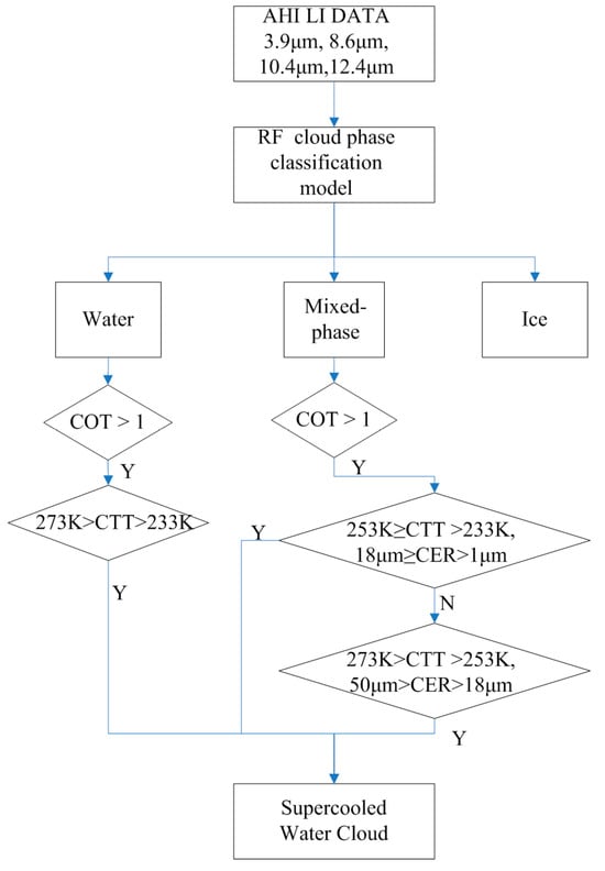
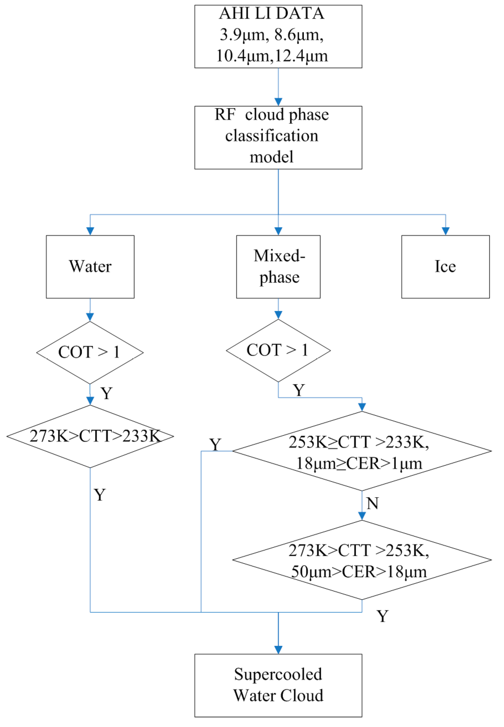
After the phase of the cloud pixel is classified, the SWC pixels can be identified with the help of the Level 2 data from H-8 products, such as COT, CTT and CER, which is quite similar to the work by Wang et al. (2019) [16]. The whole flowchart of SWC identification is shown in Figure 1. When the cloud is identified as a water cloud or mixed-phase cloud, it will flow into the next stage to be further discriminated. Using COT and CTT, the water cloud will be classified into SWCs and warm clouds. With the addition of CER, mixed-phase clouds can further be identified as SWCs or not.

Figure 1. This is the flowchart for SWC identification.

SWC pixels are predominantly observed in optically thick cloud regions. The identification of potential supercooled water cloud (SWC) pixels is closely linked to cloud physical thickness [27]. Following Minnis et al. (1995), cloud physical thickness can be inferred from the combined use of cloud optical thickness (COT) and cloud-top temperature (CTT), with thickness increasing monotonically with COT at a given CTT [28]. Consistent with Wang et al. (2019) [16], the minimum COT threshold of 1 is selected to detect SWC pixels.

According to the definition of SWCs, the water clouds below 0 °C can be considered SWCs. Hence, using the threshold of CTT, warm water clouds and supercooled water clouds can be easily identified by differentiating their cloud-top temperature. Here, we restrict the cloud-top temperature to 0 °C to −40 °C (273 K~233 K), since supercooled liquid water generally undergoes homogeneous freezing and transitions to ice at temperatures colder than −40 °C [5].

Besides the water clouds below 0 °C, SWCs can also exist in “mixed-phase” clouds according to the model output. Since ice-above-water, water-above-ice, and mixed-phase layers are all labeled indiscriminately as “mixed-phase clouds” in the model output, and apparently SWCs exist in the water-above-ice and mixed-phase layer situations, it is necessary to identify the ice-above-water cases for accurate SWC retrieval. As the water layer under ice can be warm water or supercooled water, it is difficult to use the particle radiative properties to differentiate them. According to in situ measurements, the homogeneous freezing of large droplets typically occurs at temperatures as high as −19 °C [29] and −21 °C [30], representing the warmest temperatures at which homogeneous freezing occurs. It was also observed that a liquid-to-ice phase transition occurs at−20 °C at an altitude of 8 km [31]. Hence, the cloud-top temperature around −20 °C can be used as a threshold for determining whether droplets of a certain diameter remain in or transit between phases. According to the work of Rosenfeld et al. (2006) [32], in adiabatic LWCs at −38 °C, the radius of supercooled droplets remains below the 50 μm threshold. The work by Wang et al. (2019) [16] shows that the CER distribution of supercooled droplets in liquid- and mixed-phase clouds exhibits distinct characteristics. Liquid-phase clouds are predominantly concentrated at smaller radii (peaking below 10 μm), whereas mixed-phase clouds show a broader distribution extending to larger radii. The 18 μm threshold effectively separates the two phases, with CER values largely below this limit in liquid clouds and frequently exceeding it in mixed-phase clouds [16]. Hence, −20 °C(253 K) and 18 μm are selected as the thresholds of CTT and CER respectively. With the thresholds of COT, CTT and CER, the SWCs can be preferentially distinguished from the “mixed-phase clouds” category in the RF model output. That is, water-above-ice and mixed-phase layers are successively and sequentially detected from the mixed-phase cloud category, as shown in Figure 1.

Figure 1 is a flowchart illustrating the systematic methodology for identifying SWCs. The overall workflow integrates multi-spectral observations with machine learning and physical thresholding to systematically identify SWCs. Initially, four thermal infrared bands (3.9 μm, 8.6 μm, 10.4 μm, and 12.4 μm) from the Himawari-8 AHI Level 1 products are fed into a random forest (RF) classifier, which performs a primary categorization of cloud pixels into three macro-phases: water, “mixed-phase”, and ice. Following this initial classification, a series of physically constrained threshold filters are applied to extract SWCs from the water and “mixed-phase” branches. For pixels initially classified as water clouds, the algorithm retains those satisfying the criteria of COT > 1 and CTT ranging between 233 K and 273 K. For the “mixed-phase” branch, the identification is refined through two sequential checks: pixels are classified as SWCs if they meet the condition of 253 K ≥ CTT > 233 K combined with 18 μm ≥ CER > 1 μm, or alternatively, if they satisfy 273 K > CTT > 253 K combined with 50 μm > CER > 18 μm, provided COT > 1 is met in both cases. Pixels classified as ice clouds by the RF model are excluded from further processing. Consequently, the final output converges all qualified pathways to delineate the spatial distribution of SWCs.

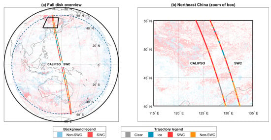
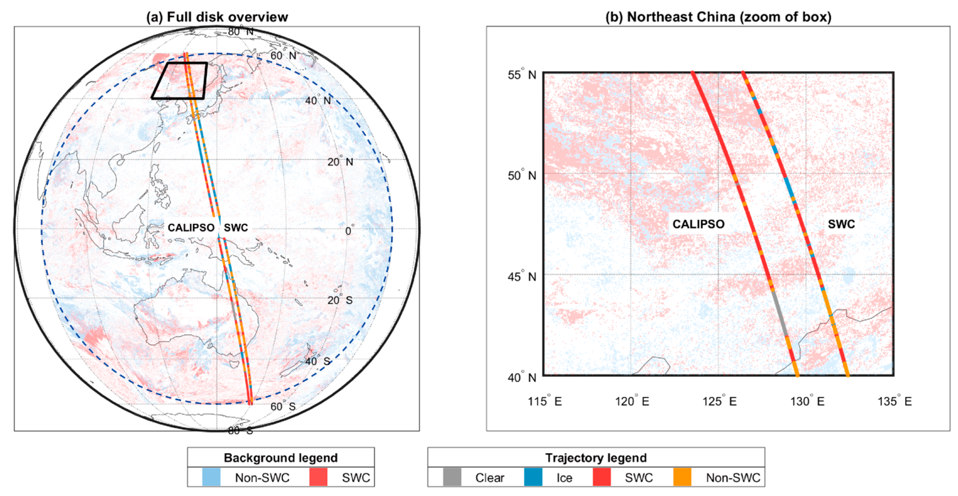
The SWC dataset served as the reference to assess the performance of the proposed identification algorithm. The spatial distribution of validation samples along CALIPSO tracks is shown in Figure 2. Here, blue and red pixels represent ice and supercooled water clouds, respectively, where the H-8 cloud-top phase retrievals match those from the CALIPSO VFM products. The false alarm rate (FAR), hit rate (HR), bias and Brier Score (BS) [33] were used to examine the performance of the detection results. The false alarm rate (FAR) and hit rate (HR)are shown in Equations (7) and (8). The FAR represents the fraction of pixels that are misclassified as SWCs, and the HR suggests the probability of correctly identifying SWCs.

$$FAR={\displaystyle \frac{AH{I}_{SWC}\&CALIPS{O}_{non-SWC}}{AH{I}_{SWC}}}$$

(7)

$$HR={\displaystyle \frac{N_{SWC}+N_{non-SWC}}{N_{collocated}}}$$

(8)

where $FAR$ is the false alarm rate, $HR$ is the hit rate, $AH{I}_{SWC}$ is the number of SWC pixels in AHI SWC detections and $CALIPS{O}_{non-SWC}$ is the number of non-SWC pixels in CALIPSO results. “&” indicates the pixels in agreement. $N_{SWC}$ is the number of SWC pixels in agreement, $N_{non-SWC}$ is the number of non-SWC pixels in agreement, and $N_{collocated}$ is the total number of collocated pixels.

Figure 2. The H-8 cloud-top phase validated against CALIPSO VFM production at 03:50 UTC on 1 January 2021.

Table 3 presents the validation statistics of the supercooled water cloud (SWC) identification results for 10 CALIOP orbit tracks sampled on 1 January, 1 May, 1 July, and 1 October. For each track, the hit rate (HR) and false alarm rate (FAR) are listed, with AVE denoting the average value across all tracks.

Table 3. SWC identification test results.

CALIOP Orbit Track	Total Pixel Numbers	HR (%)	FAR (%)	Bias	BS
Track 1 (1 January)	63,120	90.8	13.0	1.043	0.0915
Track 2 (1 January)	63,360	89.5	10.6	1.001	0.0966
Track 3 (1 January)	63,360	91.7	15.7	1.088	0.0876
Track 1 (1 May)	63,360	96.3	30.8	1.391	0.1236
Track 2 (1 May)	63,360	89.0	14.3	1.039	0.0830
Track 3 (1 May)	63,120	82.9	22.7	1.073	0.1372
Track 1 (1 July)	62,880	80.7	60.8	2.058	0.1218
Track 2 (1 July)	62,880	95.7	12.8	1.098	0.0850
Track 1 (1 October)	63,840	91.5	5.3	0.966	0.1078
Track 2 (1 October)	63,600	84.4	20.5	1.062	0.2240
AVE		89.3	20.7	1.182	0.1158

Overall, the proposed method achieves an average Hit Rate (HR) of 89.3%, indicating generally high detection capability for SWCs, alongside an average false alarm rate (FAR) of 20.7%, a bias of 1.182, and a Brier score of 0.1158, suggesting a moderate level of misclassification. While performance remains relatively stable in January, with HRs ranging from 89.5% to 91.7% and FARs mostly below 16%, noticeable variability emerges across months and individual tracks. The HR spans from 80.7% (Track 1, 1 July) to 96.3% (Track 1, 1 May), while the FAR fluctuates dramatically from 5.3% (Track 1, 1 October)—where Bias is closest to unity (0.966), indicating precise detection—to a pronounced spike of 60.8% (Track 1, 1 July), accompanied by a Bias of 2.058 reflecting substantial over-prediction. This particularly high FAR in early July implies increased difficulty in discriminating SWCs during that period, possibly due to complex cloud phase conditions or greater contamination by ice and mixed-phase clouds. In contrast, the consistently high HR values in January and May, coupled with the low FAR in October, demonstrate more reliable identification under those conditions.

4. SWCs in the NCCV

As a mid-latitude cutoff low situated in the mid- to upper troposphere, NCCV can develop all year round, yet its activity peaks predominantly from late spring to early summer [11]. Intense NCCV episodes are frequently associated with extreme precipitation, cold anomalies, and severe convective storms across Northeast and East China [34]. These impacts are particularly pronounced during its climatological peak from May to mid-June [35]. For example, strong tornado events in Suzhou and Wuhan and a hailstorm that struck Jiangxi province in May 2021 were closely related to the persistent NCCV activity background [36]. The spatial distribution of supercooled liquid water (SLW) clouds serves as a critical microphysical nexus linking the macroscale circulation of NCCV to its surface impacts. Specifically, the large-scale dynamics (e.g., frontal lifting and moisture transport) determine the formation and geographical extent of SLW within the NCCV system. In turn, the spatial heterogeneity of SLW—such as its horizontal extent and vertical overlap with ice phases—modulates the cloud radiative effect and precipitation efficiency, which directly dictate the surface temperature and hydrological response. Hence, characterizing the spatial distribution features of SWCs in the NCCV is essential not only for mapping their occurrence but also for elucidating the mechanisms through which NCCV influences surface weather and climate.

This study investigates the SWCs in the NCCV activity during late spring (April–May) 2021. According to the definition by Sun et al. (1994) [11], there were 43 NCCV days in that period. Using the SWC identification method presented in this work, the SWC distributions in NCCV between April and May 2021 were identified. The study region (35–60°N, 115–145°E) was partitioned into four quadrants relative to the center point (47.5°N, 130°E). Combined with cloud phase products and vertical stratification into low, middle, and high levels, statistical analyses were conducted for the 02:00, 06:00, and 10:00 UTC time steps to elucidate the spatial distribution and diurnal evolution of supercooled water clouds.

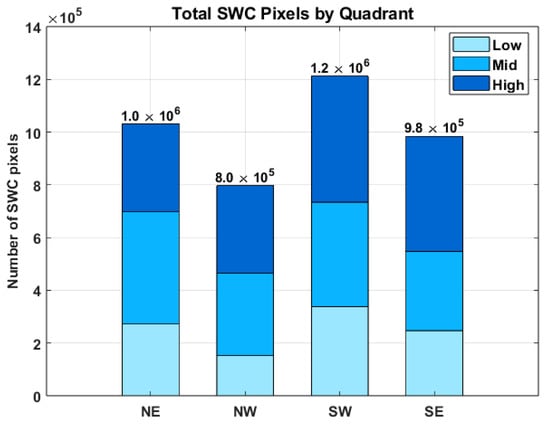
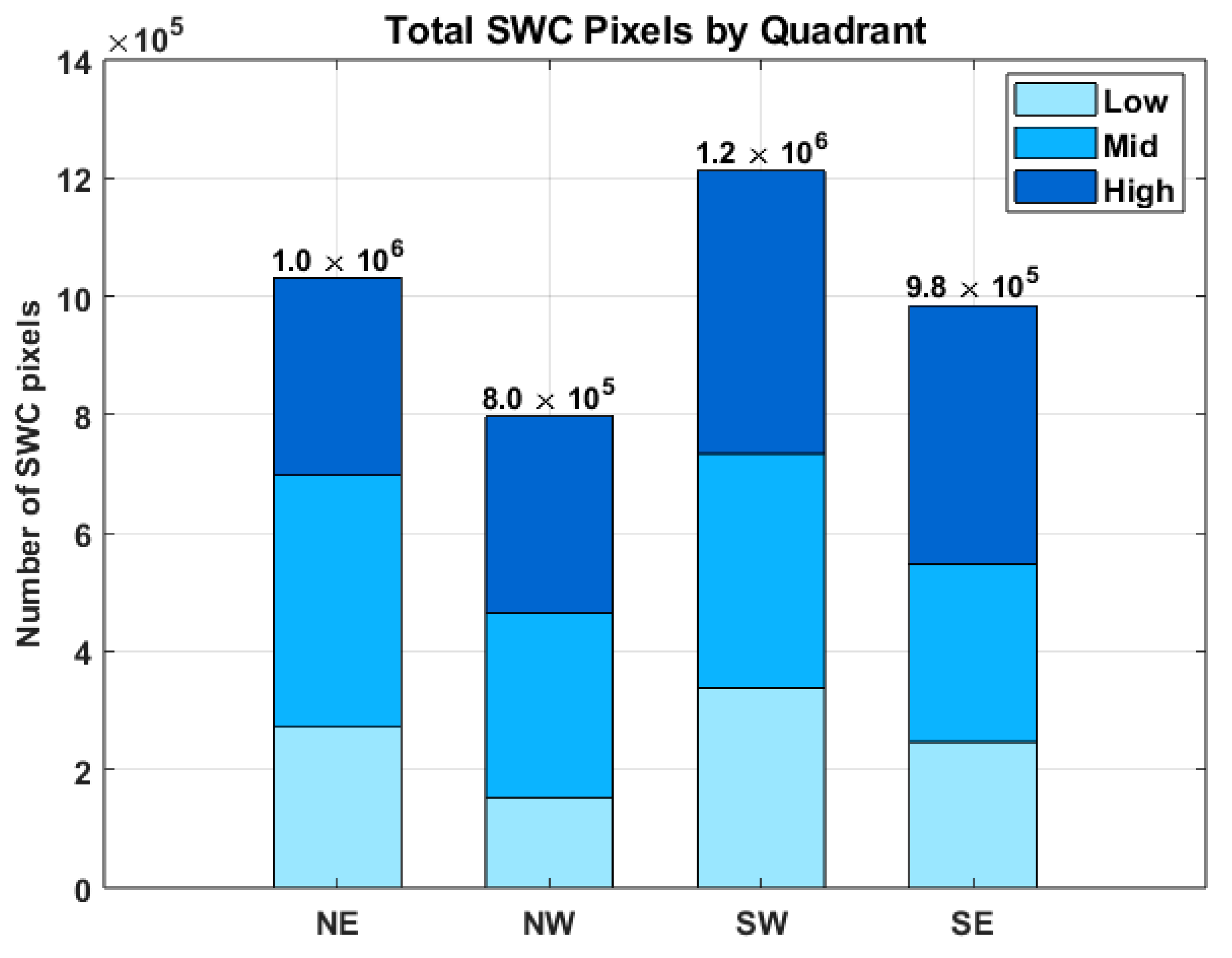
Significant spatial disparities in the extent of supercooled water clouds exist among the quadrants of the NCCV (Figure 3). The southwest quadrant exhibits the highest total pixel count (approximately 1.2 × 10⁶), identifying it as the most enriched region for supercooled water clouds. The northeast and southeast quadrants follow closely, with comparable totals (1.0 × 10⁶ and 9.8 × 10⁵, respectively), while the northwest quadrant records the lowest total (approximately 8.0 × 10⁵). Across all quadrants, high-level clouds contribute the most to the SWCs, followed by mid-level clouds, with low-level clouds making the smallest contribution. Overall, a distinct spatial pattern of “higher in the southwest and lower in the northwest” is observed.

Figure 3. Distribution characteristics of supercooled water clouds across different quadrants of NCCV activity during late spring (April–May) 2021.

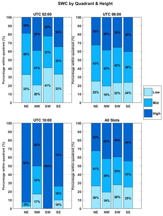
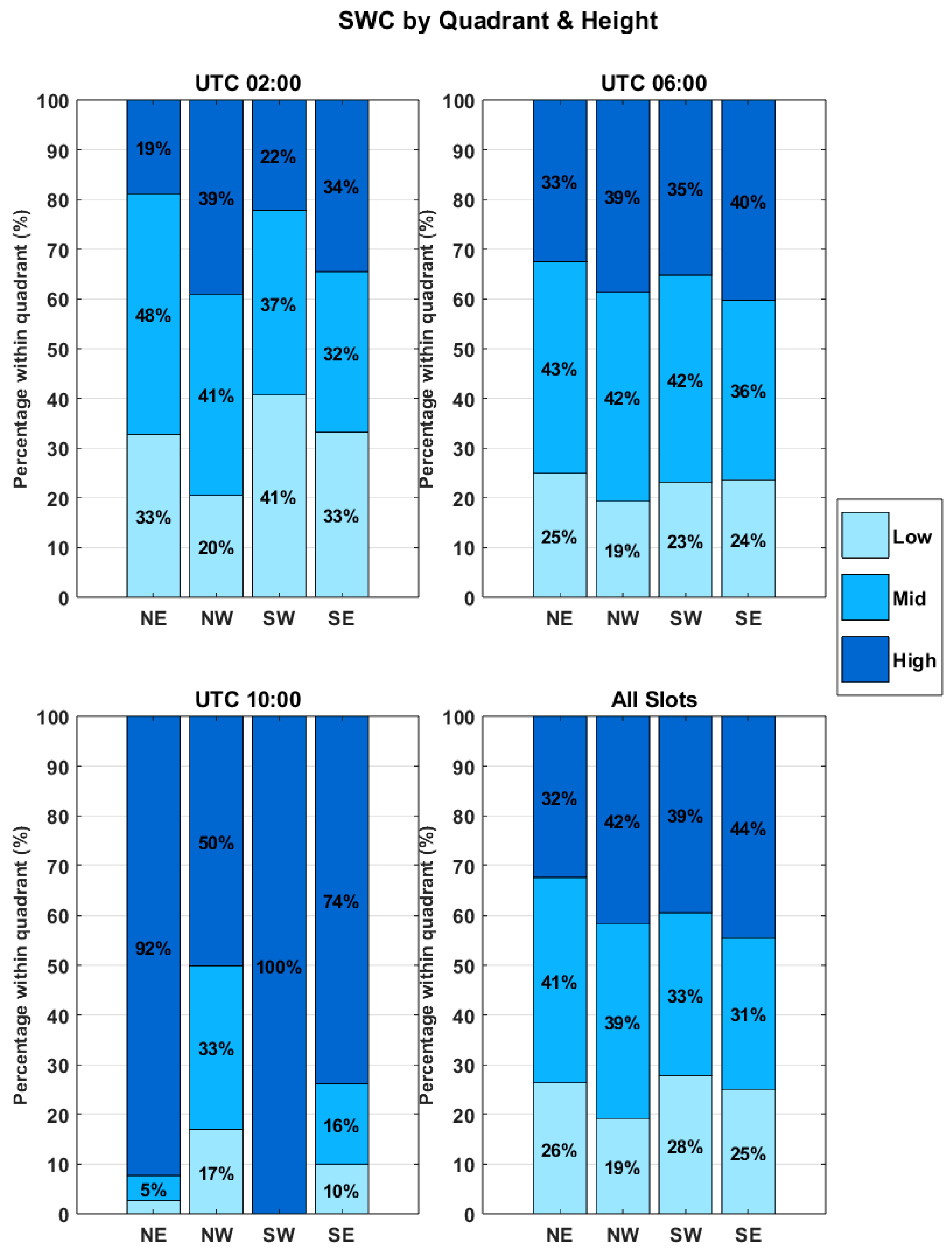
Figure 4 shows the vertical distribution and diurnal variation in supercooled water clouds associated with the NCCV. The vertical structure of supercooled water clouds exhibits distinct diurnal evolution, characterized by a persistent upward shift from the middle and low levels to the high level throughout the day, as shown in Figure 4.

Figure 4. Vertical distribution and diurnal variation in supercooled water clouds during NCCV activity in late spring (April–May) 2021.

At 02:00 UTC (10:00 BT, morning), supercooled water clouds were relatively concentrated in the mid- and low-level layers. The northeast quadrant exhibited the highest proportion of mid-level clouds (48%), while the southwest quadrant recorded the highest low-cloud fraction across the entire domain (41%). Distributions across the three vertical levels in the northwest and southeast quadrants remained relatively balanced.

By 06:00 UTC (14:00 BT, afternoon), the vertical centroid of the cloud mass shifted progressively upward, with high-cloud fractions increasing and low-cloud fractions decreasing across all quadrants. This shift was most pronounced in the southwest quadrant, where the low-cloud fraction dropped to 23% and the high-cloud fraction rose to 35%.

At 10:00 UTC (18:00 BT, evening), high-level clouds became the dominant component of supercooled water clouds. The high-cloud fractions in the southwest and northeast quadrants reached nearly 100% and 92%, respectively, accompanied by a substantial dissipation of supercooled water in the mid- and low-level layers. In the southeast and northwest quadrants, high-cloud fractions accounted for 74% and 50%, respectively, representing the largest contributions within these sectors.

Aggregated statistics for the entire period indicate that high-level clouds contributed the most to supercooled water content in the northwest, southwest, and southeast quadrants (39–44%), whereas mid-level clouds dominated in the northeast quadrant (41%). Low-cloud fractions remained within the range of 19–28% across all regions.

In summary, supercooled water clouds under the influence of the Northeast Cold Vortex exhibit significant spatial heterogeneity and distinct diurnal vertical evolution. Spatially, the southwest quadrant is characterized by the highest total abundance and the most intense diurnal variability, while the northwest quadrant shows the lowest total abundance and a relatively stable vertical structure. Temporally, a consistent upward migration occurs from morning to evening, indicating an evolutionary pattern wherein supercooled water shifts progressively from mid- and low-level layers to the high-level layer.

5. Conclusions

Accurate identification of SWCs is essential for weather modification, aviation safety, and climate research. In this study, we developed a two-step algorithm to detect SWCs using observations from the AHI onboard Himawari-8. The first step employed a RF model to classify clouds into nine categories—high ice, high water, high mixed, middle ice, middle water, middle mixed, low water, low ice, and low mixed clouds—based on four Level-1 infrared bands (3.9, 8.6, 10.4, and 12.4 μm). The second step further identified SWCs from the water and mixed-phase clouds by integrating AHI Level-2 products, including COT, CER, and CTT.

The algorithm was rigorously validated against collocated CALIPSO VFM data. Results demonstrated an overall hit rate of 89.3% across 632,880 validated pixels, confirming the high detection capability of the proposed method. Although the average false alarm rate was 20.7%, with notably higher values in July, the algorithm generally satisfied the accuracy requirements for operational cold-cloud seeding and precipitation enhancement.

Applying the validated algorithm to late spring (April–May) 2021 NCCV events, we revealed pronounced spatial heterogeneity and distinct diurnal vertical evolution of SWCs. The southwest quadrant of the NCCV consistently exhibited the highest SWC abundance (approximately 1.2 × 10⁶ pixels), forming a “higher in the southwest and lower in the northwest” spatial pattern. Diurnally, SWCs underwent a progressive upward migration: they were initially concentrated in mid- and low-level layers during the morning (02:00 UTC), and gradually shifted to the high-level layer by evening. These findings provide valuable observational constraints for understanding cloud microphysical processes within cold vortices and offer practical guidance for optimizing weather modification operations in Northeast China.

Future work should focus on reducing the false alarm rate, particularly during summer months, by incorporating additional spectral bands or advanced machine learning techniques. Moreover, extending the algorithm to other geostationary satellites could enable broader monitoring of SWCs, ultimately supporting improved precipitation efficiency and aviation safety on a global scale.

References

- Dufresne, J.L.; Bony, S. An assessment of the primary sources of spread of global warming estimates from coupled atmosphere ocean models. J. Clim. 2008, 21, 5135–5144. [Google Scholar] [CrossRef] [Scilit]
- Stephens, G.L.; Li, J.; Wild, M.; Clayson, C.A.; Loeb, N.; Kato, S.; L’Ecuyer, T.; Stackhouse, P.W., Jr.; Lebsock, M.; Andrews, T. An update on Earth’s energy balance in light of the latest global observations. Nat. Geosci. 2012, 5, 691–696. [Google Scholar] [CrossRef] [Scilit]
- Lawson, R.P.; Gettelman, A. Impact of Antarctic mixed-phase clouds on climate. Proc. Natl. Acad. Sci. USA 2014, 111, 18156–18161. [Google Scholar] [CrossRef] [Scilit] [PubMed]
- Tan, I.; Storelvmo, T.; Zelinka, M.D. Observational constraints on mixed-phase clouds imply higher climate sensitivity. Science 2016, 352, 224–227. [Google Scholar] [CrossRef] [Scilit] [PubMed]
- Korolev, A.; McFarquhar, G.; Field, P.R.; Franklin, C.; Lawson, P.; Wang, Z.; Williams, E.; Abel, S.J.; Axisa, D.; Borrmann, S.; et al. Mixed-Phase Clouds: Progress and Challenges. Meteor. Mon. 2017, 58, 51–550. [Google Scholar] [CrossRef] [Scilit]
- Marchant, B.; Platnick, S.; Meyer, K.; Arnold, G.T.; Riedi, J. MODIS Collection 6 shortwave-derived cloud phase classification algorithm and comparisons with CALIOP. Atmos. Meas. Tech. 2016, 9, 1587–1599. [Google Scholar] [CrossRef] [Scilit] [PubMed]
- Murray, B.J.; O’Sullivan, D.; Atkinson, J.D.; Webb, M.E. Ice nucleation by particles immersed in supercooled cloud droplets. Chem. Soc. Rev. 2012, 41, 6519. [Google Scholar] [CrossRef] [Scilit] [PubMed]
- Xu, X.; Zeng, Y.; Yu, X.; Liu, G.; Yue, Z.; Dai, J.; Feng, Q.; Liu, P.; Wang, J.; Zhu, Y. Identification of Supercooled CloudWater by FY-4A Satellite and Validation by CALIPSO and Airborne Detection. Remote Sens. 2023, 15, 126. [Google Scholar] [CrossRef] [Scilit]
- Cober, S.G.; Isaac, G.A. Characterization of Aircraft Icing Environments with Supercooled Large Drops for Application to Commercial Aircraft Certification. J. Appl. Meteorol. Clim. 2012, 51, 265–284. [Google Scholar] [CrossRef] [Scilit]
- Song, J. Northeast China cold vortex: Three-dimensional structure, life cycle, and dynamical understanding. J. Meteor. Res. 2026, 40, 732–748. [Google Scholar] [CrossRef] [Scilit]
- Sun, L.; Zheng, X.; Wang, Q. The climatological characteristics of northeast cold vortex China. Q. J. Appl. Meteorol. 1994, 5, 297–303. (In Chinese) [Google Scholar]
- Liu, C.; Fang, Y.; Zhang, K.; Li, Y.; Wang, Y. Northeast China cold vortex is the key factor influencing the high-impact agroclimatic events in Northeast China. Dynam. Atmos. Ocean. 2024, 107, 101477. [Google Scholar] [CrossRef] [Scilit]
- Guo, J.P. Advances in impacs of climate change on agricultural production in China. J. Appl. Meteorol. Sci. 2015, 26, 1–11. [Google Scholar]
- Qi, Y.B.; Guo, X.L.; Jin, D.Z. Observational study on the macro- and microphysical structure of a convective cloud band in a Northeast China cold vortex. Chin. J. Atmos. Sci. 2007, 31, 621–634. [Google Scholar]
- Bessho, K.; Date, K.; Hayashi, M.; Ikeda, A.; Imai, T.; Inoue, H.; Kumagai, Y.; Miyakawa, T.; Murata, H.; Ohno, T.; et al. An Introduction to Himawari-8/9—Japan’s New-Generation Geostationary Meteorological Satellites. J. Meteorol. Soc. Jpn. 2016, 94, 151–183. [Google Scholar] [CrossRef] [Scilit]
- Wang, Z.; Letu, H.; Shang, H.; Zhao, C.; Li, J.; Ma, R. A supercooled water cloud detection algorithm using Himawari-8 satellite measurements. J. Geophys. Res.-Atmos. 2019, 124, 2724–2738. [Google Scholar] [CrossRef] [Scilit]
- Fu, H.; Zhang, F.; Guo, B.; Li, W. Supercooled Water Cloud Identification from Geostationary Satellite Thermal Infrared Observations and Its Application in the Sun Glint Region. IEEE Trans. Geosci. Remote Sens. 2024, 62, 4110210. [Google Scholar] [CrossRef] [Scilit]
- Winker, D.M.; Vaughan, M.A.; Omar, A.; Hu, Y.; Powell, K.A. Overview of the CALIPSO mission and CALIOP data processing algorithms. J. Atmos. Ocean. Technol. 2009, 26, 2310–2323. [Google Scholar] [CrossRef] [Scilit]
- Hersbach, H.; Bell, B.; Berrisford, P.; Hirahara, S.; Horányi, A.; Muñoz-Sabater, J.; Nicolas, J.; Peubey, C.; Radu, R.; Schepers, D.; et al. The ERA5 global reanalysis. Quart. J. Roy. Meteor. Soc. 2020, 146, 1999–2049. [Google Scholar] [CrossRef] [Scilit]
- Letu, H. A new benchmark for surface radiation products over the East Asia–Pacific region retrieved from the Himawa ri-8/AHI next-generation geostationary satellite. Bull. Amer. Meteorol. Soc. 2021, 103, E873–E888. [Google Scholar] [CrossRef] [Scilit]
- Wang, C.; Platnick, S.; Meyer, K.; Zhang, Z.; Zhou, Y. A machine-learning-based cloud detection and thermodynamic-phase classification algorithm using passive spectral observations. Atmos. Meas. Tech. 2020, 13, 2257–2277. [Google Scholar] [CrossRef] [Scilit]
- Zhou, G.; Wang, J.; Yin, Y.; Hu, X.; Letu, H.; Sohn, B.J.; Yung, Y.L.; Liu, C. Detecting supercooled water clouds using passive radiometer measurements. Geophys. Res. Lett. 2022, 49, e2021GL096111. [Google Scholar] [CrossRef] [Scilit]
- Winker, D.M.; Hunt, W.H.; McGill, M.J. Initial performance assessment of CALIOP. Geophys. Res. Lett. 2007, 34, L19803. [Google Scholar] [CrossRef] [Scilit]
- Hu, Y. and Coauthors: CALIPSO/CALIOP Cloud Phase Discrimination Algorithm. J. Atmos. Ocean. Technol. 2009, 26, 2293–2309. [Google Scholar] [CrossRef] [Scilit]
- Tan, Z.; Ma, S.; Liu, C.; Teng, S.; Xu, N.; Hu, X.; Zhang, P.; Yan, W. Assessing overlapping cloud top heights: An extrapolation method and its performance. IEEE Trans. Geosci. Remote Sens. 2022, 60, 4107811. [Google Scholar] [CrossRef] [Scilit]
- Breiman, L. Random Forests–Random Features; Technical report; University of California at Berkeley: Berkeley, CA, USA, 1999. [Google Scholar]
- Roskovensky, J.K.; Ivey, I.; Porch, W.; Beavis, N.; Hermann, R.; Silber, S. Cloud super-cooled liquid water estimation from satellite data. J. Weather Modif. 2011, 43, 64–82. [Google Scholar] [CrossRef] [Scilit]
- Minnis, P.; Smith, W.L.; Garber, D.P.; Ayers, J.K.; Doelling, D.R. Cloud Properties Derived from GOES-7 for Spring 1994 ARM Intensive Observing Period Using Version 1.0.0 of ARM Satellite Data Analysis Program; NASA Reference Publication1366; NASA Langley Research Center: Hampton VA, USA, 1995. [Google Scholar]
- Ikeda, K.; Rasmussen, R.M.; Hall, W.D.; Thompson, G. Observations of freezing drizzle in extratropical cyclonic storms during IMPROVE-2. J. Atmos. Sci. 2007, 64, 3016–3043. [Google Scholar] [CrossRef] [Scilit]
- Cober, S.G.; Isaac, G.A.; Strapp, J.W. Characterizations of aircraft icing environments that include supercooled large drops. J. Appl. Meteorol. 2001, 40, 1984–2002. [Google Scholar] [CrossRef] [Scilit]
- Yorks, J.E.; Hlavka, D.L.; Hart, W.D.; McGill, M.J. Statistics of cloud optical properties from airborne lidar measurements. J. Atmos. Ocean. Technol. 2011, 28, 869–883. [Google Scholar] [CrossRef] [Scilit]
- Rosenfeld, D.; Woodley, W.L.; Krauss, T.W.; Makitov, V. Aircraft microphysical documentation from cloud base to anvils ofhailstorm feeder clouds in Argentina. J. Appl. Meteorol. Climatol. 2006, 45, 1261–1281. [Google Scholar] [CrossRef] [Scilit]
- Mace, G.G.; Jakob, C.; Moran, K.P. Validation of hydrometeor occurrence predicted by the ECMWF model using millimeter wave radar data. Geophys. Res. Lett. 1998, 25, 1645–1648. [Google Scholar] [CrossRef] [Scilit]
- Xie, Z.; Bueh, C. Different types of cold vortex circulations over Northeast China and their weather impacts. Mon. Weather Rev. 2015, 143, 845–863. [Google Scholar] [CrossRef] [Scilit]
- Xie, Z.; Bueh, C. Low frequency features of northeastern China cold vortex and its background circulation pattern. Acta Meteorol. Sin. 2012, 70, 704–716. [Google Scholar]
- Wu, J.; Liu, Y.; Li, Y.; Zuo, J.; Nie, Y.; Li, Q.; Zhang, S.; Wang, D. The extreme Northeast China cold vortex activities in the late spring of 2021 and possible causes involved. Adv. Clim. Change Res. 2022, 13, 787–796. [Google Scholar] [CrossRef] [Scilit]
Disclaimer/Publisher’s Note: The statements, opinions and data contained in all publications are solely those of the individual author(s) and contributor(s) and not of MDPI and/or the editor(s). MDPI and/or the editor(s) disclaim responsibility for any injury to people or property resulting from any ideas, methods, instructions or products referred to in the content. |
© 2026 by the authors. Licensee MDPI, Basel, Switzerland. This article is an open access article distributed under the terms and conditions of the Creative Commons Attribution (CC BY) license.