Mapping Active Surface Deformation in Fusagasugá and Silvania, Colombia, Using Sentinel-1 SBAS-InSAR and Campaign GNSS Observations

Highlights

What are the main findings?

• SBAS-InSAR identified spatially coherent LOS deformation in three poorly monitored rural sectors of Fusagasugá and Silvania, Colombia.
• The strongest signal occurred at El Bermejal, where descending LOS velocities reached approximately −31 mm/year during 2020–2021.

What are the implications of the main findings?

• Campaign GNSS provides complementary point-scale observations but does not independently validate the spatially averaged InSAR time series.
• The workflow provides a transferable regional screening framework for prioritizing field, geodetic, and geotechnical investigations in data-scarce mountainous regions.

Abstract

The municipalities of Fusagasugá and Silvania in Cundinamarca, Colombia, include rural mountainous terrain and infrastructure exposed to hydrometeorological and geological hazards, yet spatially continuous ground-deformation measurements remain limited. We mapped surface deformation using ascending and descending Sentinel-1 Small Baseline Subset Interferometric Synthetic Aperture Radar (SBAS-InSAR) observations acquired during 2020–2021 and compared local InSAR time series with four-epoch campaign GNSS measurements at four sites. The InSAR analysis identifies spatially coherent line-of-sight (LOS) deformation in San Antonio, San Luis Bajo, and El Bermejal. At P2 in San Antonio, the full-period linear trends of the coherence-weighted local InSAR time series are +4.7 mm/year for the ascending geometry and −17.8 mm/year for the descending geometry; descending LOS velocities reach approximately −31 mm/year at El Bermejal. At San Antonio, inversion of paired ascending and descending LOS velocities, assuming negligible north–south motion, yields $d_E=-18.3$ mm/year (18.3 mm/year westward) and $d_U=-8.4$ mm/year (8.4 mm/year downward). GNSS-to-LOS comparisons show substantial discrepancies at P2 and P4 and inconclusive agreement at P3; campaign GNSS is therefore treated as complementary point-scale evidence rather than as independent validation of the InSAR time series. The resulting deformation maps provide a screening basis for prioritizing follow-up geodetic, geomorphological, and geotechnical investigations rather than constituting landslide-susceptibility, hazard, risk, or early-warning products.

1. Introduction

Landslides and mass movements are among the natural hazards with the greatest impact on infrastructure, human settlements, and territorial development [1]. Their occurrence and frequency have increased in many mountainous regions as a result of climate variability, land-cover change, deforestation, agricultural expansion, and uncontrolled urbanization. These processes generate significant economic losses and casualties every year [2,3], and their impacts are particularly severe in regions where settlements, roads, productive activities, and critical infrastructure are located on unstable slopes. Landslide occurrence is controlled by the interaction of geological, geomorphological, hydrological, climatic, and anthropogenic factors; therefore, their dynamics, triggering mechanisms, spatial distribution, and consequences vary considerably from one region to another [2,3,4,5,6,7,8].

Colombia is highly prone to landslides and mass movements, especially in the Andean region, where steep topography, intense rainfall, active tectonics, and complex geological conditions favor slope instability [9]. These events have produced substantial economic and social impacts by affecting transportation networks, civil works, agricultural activities, rural settlements, and, in some cases, human life [10]. In recent decades, the susceptibility of many Colombian mountainous areas has been further intensified by climate variability and continuous human intervention in natural systems. Deforestation, expansion of the agricultural frontier, inadequate watershed management, and poorly controlled urbanization have modified slope conditions and increased exposure to hydro-meteorological and geological hazards. These local factors are superimposed on broader geodynamic processes, including fault systems, volcanic activity, and plate tectonics, which also condition the regional distribution of instability processes.

In this context, terrain monitoring can contribute evidence to landslide investigations and future warning strategies [11]. Deformation measurements describe the spatial distribution, temporal evolution, and magnitude of surface motion and can therefore help prioritize locations for detailed investigation. They do not, by themselves, establish landslide susceptibility, hazard, or risk, which additionally require conditioning-factor, process, temporal-probability, and exposure information. In Colombia, public institutions have strengthened the compilation, processing, and dissemination of geospatial and hazard-related information to support risk prevention and territorial planning [12]. However, in many rural and mountainous areas, systematic deformation measurements are still scarce, and the spatial coverage of ground-based monitoring networks remains limited.

Satellite radar interferometry, particularly Interferometric Synthetic Aperture Radar (InSAR), has become one of the most widely used remote-sensing techniques for detecting and monitoring ground deformation associated with landslides. By exploiting the phase difference between repeated SAR acquisitions, InSAR can map line-of-sight (LOS) surface displacements over large areas with dense spatial sampling and millimetric-to-centimetric sensitivity under favorable conditions [13,14,15,16]. Among time-series InSAR approaches, the Small Baseline Subset InSAR (SBAS-InSAR) technique limits temporal and perpendicular baselines to reduce decorrelation and is often useful in rural and semi-vegetated environments.

Despite these advantages, the use of InSAR for systematic landslide-related deformation monitoring in Colombia remains limited. This gap is particularly relevant in the municipalities of Fusagasugá and Silvania, located in the department of Cundinamarca, where official information indicates that 69.98% and 99.9% of their territories, respectively, are exposed to hydro-meteorological and geological hazards. These municipalities include rural areas, scattered settlements, agricultural land, road corridors, fault-controlled structures, and slopes affected by rainfall-driven instability processes [9]. Nevertheless, detailed spatiotemporal information on active deformation in these areas is still insufficient.

The objective of this study is to evaluate the applicability of Sentinel-1 SBAS-InSAR for detecting, delimiting, and quantifying surface deformation potentially associated with slope instability in Fusagasugá and Silvania. The analysis uses ascending and descending Sentinel-1 datasets and compares local LOS time series with campaign GNSS observations at four control points. The work provides a spatiotemporal characterization of deformation in rural sectors of the Sumapaz region, while explicitly evaluating the effects of LOS geometry, sparse GNSS sampling, spatial averaging, and measurement uncertainty. Rather than producing a susceptibility classification, which would require a landslide inventory and conditioning-factor model, this study provides a deformation-based screening framework for prioritizing sectors for targeted geodetic, geomorphological, and geotechnical investigation.

In contrast to susceptibility-modelling studies conducted elsewhere in the Colombian Andes [9], this study provides time-series measurements of active surface deformation in a poorly monitored rural region where spatially continuous deformation information was previously unavailable. Its contribution is therefore not a new SBAS-InSAR algorithm, but a reproducible deformation-screening framework that explicitly accounts for viewing geometry, spatial coherence, local averaging, and the limitations of sparse campaign GNSS observations. This framework is transferable to other data-scarce, vegetated mountainous regions, where it can support the prioritization of field surveys and denser geodetic or geotechnical monitoring.

The remainder of this paper is organized as follows. Section 2 describes the study area and its geological, geomorphological, and hydroclimatic context. Section 3 presents the datasets and methodology, including Sentinel-1 SBAS-InSAR processing and GNSS observations. Section 4 reports the deformation results for the main unstable sectors identified in the study area. Section 5 discusses the implications, limitations, and potential applications of the results, and Section 6 summarizes the main conclusions.

2. Study Area

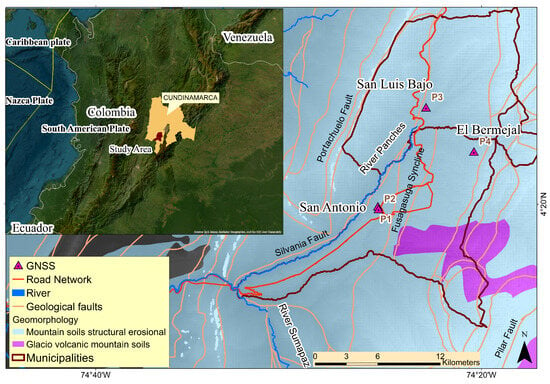
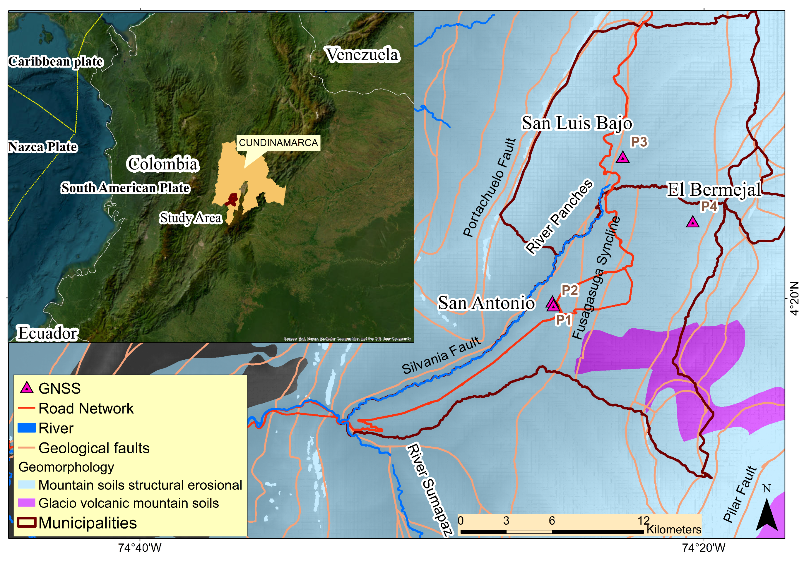
The municipalities of Fusagasugá and Silvania are located in the province of Sumapaz, which belongs to the department of Cundinamarca, Colombia. This region is characterized by its high agricultural and livestock density, made up mainly of smallholdings that support an economy based on food production and livestock activities. The region also has important road corridors that facilitate connectivity and the transportation of products (Figure 1). Geographically, these municipalities are located on the western slope of the Eastern Cordillera of the Colombian Andes, an orogenic formation resulting from the interaction between the Nazca plate and the South American plate, a process that has given rise to a diverse topography rich in natural resources. This strategic location not only influences its economic dynamics but also its biodiversity and unique landscapes, which combine mountains, valleys, and areas of high productivity.

Figure 1. Location and geological context of the study area in the municipalities of Fusagasugá and Silvania, Cundinamarca, Colombia. The inset shows the location of the study area within Colombia and its regional tectonic setting. Dark-red outlines delimit the municipalities. The map also shows the road and river networks, the principal geological faults, the Fusagasugá Syncline, and the three investigated sectors: San Antonio, San Luis Bajo, and El Bermejal. The GNSS observation sites P1–P4 (magenta triangles) provided complementary ground-based measurements for comparison with the SBAS-InSAR-derived deformation results.

Its orogenic process [10,17] was characterized by its dynamics and discontinuous movements in time and space, resulting in the alternation of sunken blocks and uplifted blocks, which leads to different heights in the Colombian Andean complex (eastern, central, and western mountain ranges) and the discontinuities between these and the lowlands. This generates a system of faults, an aspect that has an impact on the morphostructural development of the relief in the country [18].

In addition to the above, in the Colombian landscape, folding patterns with a north–south direction and axis are recognized, which result from the compression that occurs in the dynamics of the Nazca and South American plates, generating a series of faulted synclines and anticlines [19,20] (Figure 1), identifiable in the area of the Eastern Cordillera where the area of the municipalities object of this study is located. The Fusagasugá syncline, the Silvania fault, and the Pilar fault (Figure 1) are particularly relevant to this study, as they structurally control the tectonic processes affecting this territory. This syncline is a structure that spatially encompasses the jurisdictions of the municipalities of Fusagasugá and Silvania, and whose axis has a northeast direction. The presence of faults can be seen on its flanks.

Among the existing faults in the study area, the Fusagasugá Fault, the Quininí Fault system, as well as the Silvania, Piedras Blancas and La Aguadita faults stand out (Figure 1). These faults together make up a complex tectonic-structural system that must be taken into account in the analysis of the different processes, dynamics, and phenomena associated with the risks and threats present in these municipalities.

Regarding the lithology in these municipalities, formations from the late Cretaceous (Guaduas formation) predominate, along with outcrops from the Tertiary (Fusagasugá arenite formation) and surface formations made up of recent deposits of Quaternary origin linked to fluvio-torrential dynamics, where a tendency for the movement of materials is identified due to the slope, the high degree of fracturing, and the predominant hydric and meteorological conditions [20].

Another aspect to consider in the context of the study area is the range of altitudes of the areas in which instabilities and ground deformation processes have normally occurred. This corresponds to the medium mountain morphostructural unit (1000–2700 m above sea level, a.s.l.) in which colluvial hillside materials and those from fluvio-torrential dynamics are found on the surface, as previously mentioned, with a predominance of alterites [18].

Bioclimatically, the study area is located in the sub-Andean and Andean floors, where the temperature ranges between 17 and 23 degrees, with a bimodal regime that has maximum rainfall in the months of April and May in the first half of the year, and in the second half of the year, in the months of October and November, with October recording the maximum rainfall [21]. According to the multi annual average, the number of days with rain in the study area is between 200 and 250 days of the annual total.

In hydrogeographic terms, the drainage network of these municipalities belongs to the Sumapaz River basin (Figure 1) to which the sub-basins and micro-basins of the Cuja, Panches-Chocho, Subía, Barro Blanco, Batán and Guavio rivers, mainly, are tributaries. These sub-basins and micro-basins are integrated into the Magdalena watershed and macro-basin.

Considering data from the National Planning Department (DNP) of Colombia, based on information from the Institute of Hydrology, Meteorology and Environmental Studies (IDEAM) and the Colombian Geological Service (SGC) [22], in Fusagasugá, 69.98% of the territory presents threats from hydro-meteorological and geological phenomena associated with landslide events, slow floods, and torrential flows. In the case of Silvania, almost the entire territory (99.9%) is subject to these same dangers [22].

3. Materials and Methods

3.1. Materials

For this study, Sentinel-1 Synthetic Aperture Radar (SAR) images from the Copernicus Programme (European Space Agency, ESA) were used. Single Look Complex (SLC) products acquired in Interferometric Wide Swath (IW) mode were downloaded from the Alaska Satellite Facility (ASF) archive [23]. The ASF products contain VV and VH channels; only VV was processed. The ascending dataset includes 49 scenes acquired between 23 January 2020 and 7 December 2021, whereas the descending dataset contains 52 scenes acquired between 6 January 2020 and 14 December 2021. Table 1 summarizes the two image stacks. The complete lists of Sentinel-1 scenes for the ascending and descending geometries are provided in Tables S1 and S2, respectively, whereas the complete lists of generated interferograms are provided in Tables S3 and S4, respectively, in the Supplementary Materials.

Table 1. Sentinel-1 SLC inventory and SBAS network parameters. Relative orbit and frame refer to the ASF records. “Central ref.” is the SARscape central super-reference used by the SBAS connection graph.

Geometry	Rel. Orbit	ASF Frame	Scenes	First–Last Acquisition	Central Ref.	Interferograms
Ascending	150	1194	49	23/01/2020–07/12/2021	12/12/2020	200
Descending	69	577	52	06/01/2020–14/12/2021	24/01/2021	211

Interferometric processing was performed using ENVI SARscape version 5.7. Previous studies have applied SARscape to derive ground-deformation maps and displacement time series under suitable coherence conditions [24,25,26,27,28]. The SBAS-InSAR processing workflow and parameters used in this study are described in Section 3.2.

In parallel, GNSS observations were carried out at four sites of interest in the study area (Figure 1) using dual-frequency Topcon Hiper SR equipment (Topcon Positioning Systems, Inc., Livermore, CA, USA). In the post-processing, a global ionospheric model was applied with products from the University of Bern, the Hopfield tropospheric model [29], precise ephemeris for the 16 campaigns, and the calibration of the permanent antennas and the Topcon Hiper SR receiver. For the vertical component, the EGM2008 geoid [30] and the local CTM-12 projection for Colombia [31] were used.

Post-processing and adjustment of the GNSS data were performed using Leica Geo Office 8.4. The coordinates of the permanent stations were updated using weekly solutions of the SIRGAS reference frame. Four independent observations were acquired at each of stations P1–P4. During each campaign, data were recorded for approximately six hours at one-second intervals. Whenever data availability permitted, the adjustment used at least three continuously operating reference stations (CORS) from the Colombian National Geodetic Network, assumed to be stable within the study reference frame (Table 2).

Table 2. GNSS observation sites, measurement dates, GNSS CORS from the Colombian National Geodetic Network used for the adjustment, and their approximate distances. The selection of reference stations was based on GNSS data availability and weekly reference frame solutions, providing an overview of the spatial coverage and geometric quality of the observations.

Site Id	Reading Date	GNSS CORS	Distance (m)
P1	19/08/2021, 23/11/2021	ABCC	49,048
	19/08/2021	ABDP	39,359
	19/08/2021, 26/08/2021, 21/09/2021, 23/11/2021	BOGA	50,986
	26/08/2021, 21/09/2021	BOGT	51,007
	19/08/2021, 26/08/2021, 21/09/2021, 23/11/2021	IBAG	88,508
P2	29/06/2021, 16/08/2021	ABCC	49,188
	24/11/2021	ABDP	39,399
	29/06/2021, 16/08/2021, 22/09/2021, 24/11/2021	BOGA	51,101
	22/09/2021	BOGT	51,122
	29/06/2021, 16/08/2021	IBAG	88,606
P3	17/08/2021, 27/11/2021	ABCC	39,017
	27/11/2021	ABDP	32,008
	13/07/2021, 17/08/2021, 23/09/2021, 27/11/2021	BOGA	41,417
	13/07/2021	BOGT	41,420
	13/07/2021, 17/08/2021, 23/09/2021, 27/11/2021	IBAG	92,476
P4	14/07/2021, 18/08/2021, 26/11/2021	ABCC	39,124
	14/07/2021, 18/08/2021, 24/09/2021, 26/11/2021	BOGA	40,680
	24/09/2021	BOGT	40,711
	14/07/2021, 18/08/2021, 24/09/2021, 26/11/2021	IBAG	97,211

The standard deviations of the adjusted GNSS coordinates at each individual epoch are formal one-standard-deviation uncertainties, not uncertainties of the displacements relative to the first epoch. When uncertainties are required for relative displacements or their LOS projections, the variances of the current and reference epochs are added, assuming independent epoch solutions.

3.2. Methods

Two common strategies for constructing deformation time series are SBAS and persistent-scatterer interferometry (PSI). SBAS forms a connected network of interferograms with restricted temporal and perpendicular baselines, whereas PSI emphasizes phase-stable point targets over the full stack [32]. SBAS does not itself classify distributed scatterers; in this implementation, SARscape retained coherent measurement points after network inversion.

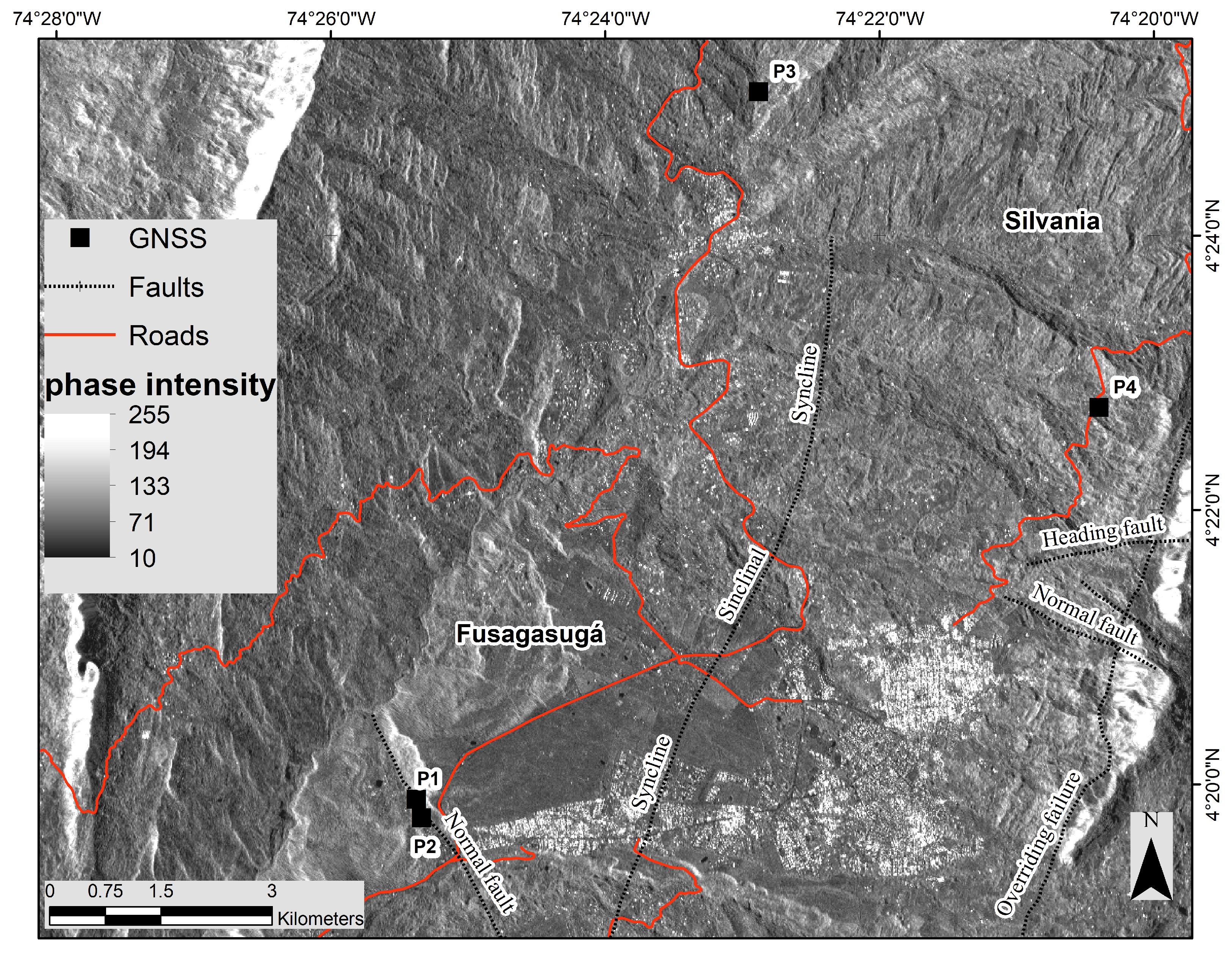
The study area (Figure 2) contains agricultural land, natural vegetation, scattered buildings, greenhouses, road corridors, and rock outcrops. Because long-baseline interferograms decorrelate readily in this heterogeneous rural setting, SBAS was selected to restrict the interferometric baselines and improve temporal-network connectivity. The resulting measurement density nevertheless varies strongly among sites and viewing geometries.

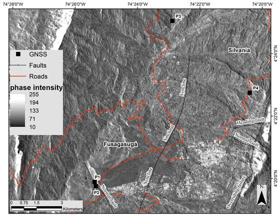
Figure 2. Sentinel-1 SAR amplitude image of the study area illustrating the locations of the GNSS stations (P1–P4, black squares), the principal geological faults (dotted line), and the road network (red lines). Pixel brightness represents the radar backscatter intensity, with high-intensity values (light tones) indicating strong radar reflectivity, whereas low-intensity values (dark tones) correspond to weak backscatter.

The SBAS-InSAR workflow is based on the generation of differential interferograms from pairs of SAR acquisitions. The processing chain includes flat-earth and topographic phase removal, adaptive interferogram filtering, phase unwrapping, and baseline refinement. The resulting interferometric network is then used to estimate incremental surface displacements, from which deformation time series and average velocity maps are derived [33].

Topographic phase removal was carried out using the 3 arc-second Shuttle Radar Topography Mission (SRTM) digital elevation model provided by NASA [34]. To preserve interferometric coherence, only image pairs separated by less than 180 days and 90 m of perpendicular baseline were considered.

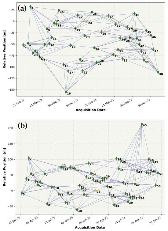
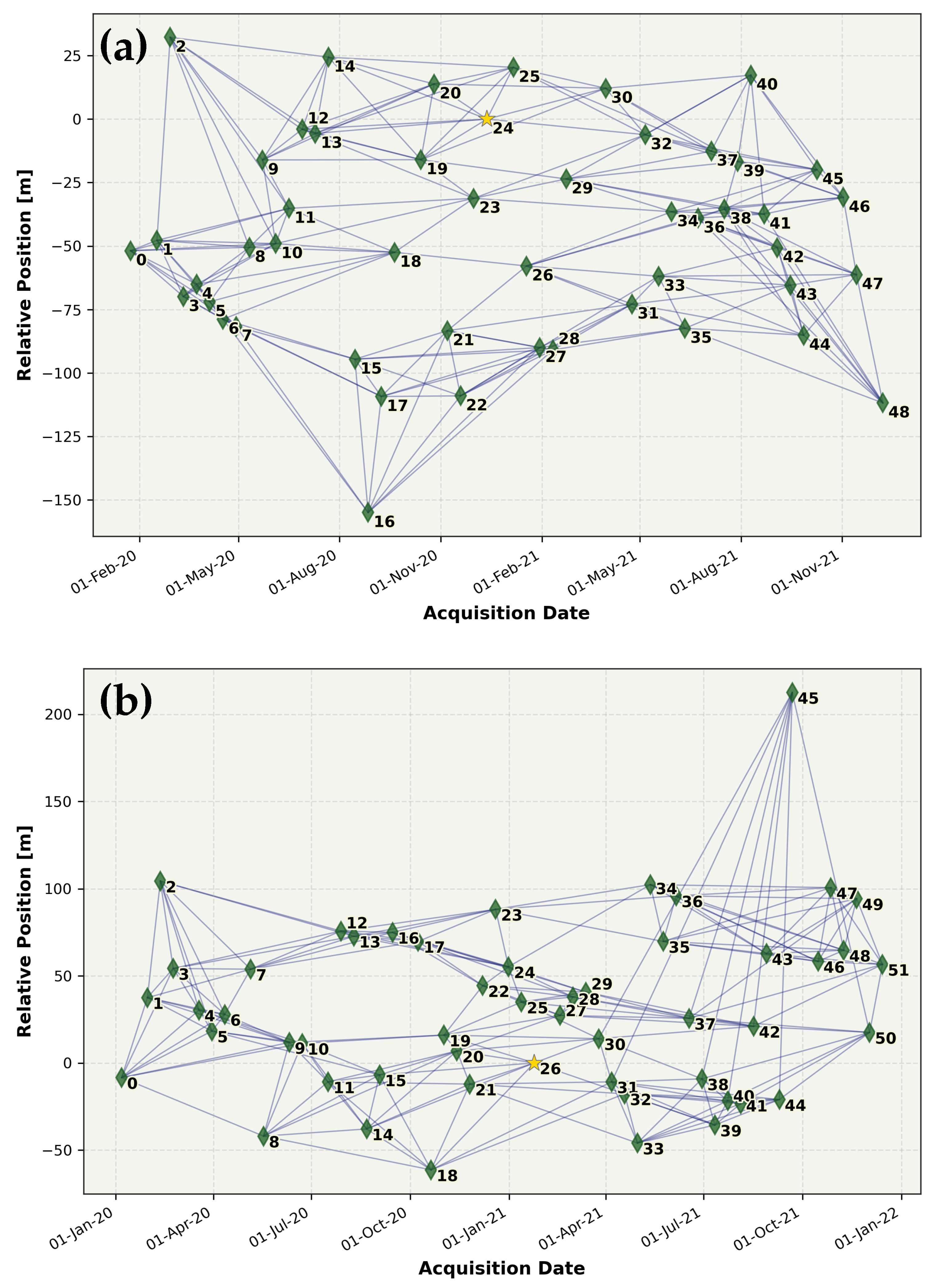
Interferometric pairs were selected in SARscape using the Connection Graph min_normal criterion, which prioritizes pairs with the smallest absolute perpendicular baselines. The network was constrained to a maximum temporal separation of 180 days and a maximum perpendicular baseline corresponding to 2% of the critical baseline, with a target of eight connections per acquisition. Applying these criteria, the ascending dataset, comprising 49 Sentinel-1 images, yielded 200 interferograms, with a mean absolute perpendicular baseline of 23.31 m (maximum: 82.83 m) and a mean absolute temporal baseline of 91.1 days. The descending dataset, comprising 52 images, produced 211 interferograms, with a mean absolute perpendicular baseline of 23.96 m (maximum: 86.11 m) and a mean absolute temporal baseline of 86.2 days. The temporal–perpendicular baseline distributions of the resulting interferometric networks are shown in Figure 3. The complete lists of ascending and descending interferograms are provided in Tables S3 and S4 of the Supplementary Materials, respectively. All 411 pairs listed in the available Connection Graph reports were marked as valid, and no additional post-selection rejection was documented.

Figure 3. SBAS interferometric networks for (a) 49 ascending scenes (relative orbit 150; central super-reference 12/12/2020) and (b) 52 descending scenes (relative orbit 69; central super-reference 24/01/2021). Yellow stars indicate the central super-reference acquisitions used by the connection graph; lines denote the interferometric pairs retained under the 180-day and 90-m baseline limits. Numbers next to the nodes are the SLC acquisition identifiers assigned by SARscape.

The interferometric networks obtained for both acquisition geometries were highly connected, with each SAR scene linked to between 8 and 11 neighboring acquisitions, which supports a stable SBAS inversion [33]. Such network redundancy improves the robustness of the inversion and reduces the impact of residual topographic errors and spatio-temporal decorrelation.

Interferograms were generated using one look in azimuth and four looks in range, resulting in approximately square ground pixels, reduced phase noise, and a modest reduction in spatial resolution. Image coregistration was initialized using precise orbit information and subsequently refined using amplitude and coherence measurements. Initial window dimensions were set to $2048\times 1024$ pixels, with a cross-correlation threshold of 0.25, a fine oversampling factor of 8, an SNR threshold of 3.2, and DEM-assisted refinement. Interferometric phase noise was reduced using the Goldstein adaptive filter, with a 64-pixel window, 80% overlap, a smoothing window of 5, and $\alpha$ values ranging from 0.3 to 2.5. Phase unwrapping was performed using the Delaunay Minimum Cost Flow algorithm with a coherence threshold of 0.3 [35]. The weighted SBAS inversion was solved using Jacobi singular value decomposition (SVD) and included a linear displacement model, residual-height estimation, and a spatial wavelet scale of 1200 m. Pixels were retained when valid measurements were available for at least 65% of the interferograms and 90% of the acquisitions.

Tropospheric phase delays were mitigated using Generic Atmospheric Correction Online Service (GACOS) products [36]. The atmospheric delay map corresponding to each Sentinel-1 acquisition was incorporated into the processing, and the differential atmospheric correction was applied to each interferometric pair before the SBAS inversion. SARscape processing parameters are listed in Table S5, while definitions and units for the exported SARscape fields used in this study are provided in Table S6 of the Supplementary Materials.

For each orbital geometry, LOS displacements were referenced to a high-coherence point exhibiting negligible displacement within the corresponding SBAS solution. The reference points were located at $(-74.3591598°,4.3312476°)$ for the ascending geometry and $(-74.4013405°,4.3155661°)$ for the descending geometry. Their coherence values were 0.999515 and 0.999472, respectively, and their estimated linear LOS velocities were effectively zero. The coordinates and associated reference-point attributes are detailed in Table S7 of the Supplementary Materials. Consequently, the reported LOS displacements and velocities are relative to the corresponding reference point in each orbital geometry.

Two complementary transformations were applied to facilitate the interpretation and comparison of the InSAR and GNSS measurements. First, ascending and descending LOS observations were combined to estimate the east–west and vertical displacement components where both viewing geometries sampled the same deformation field over comparable time intervals. Given the limited north–south sensitivity of near-polar Sentinel-1 acquisitions, this decomposition assumes that the north–south displacement component is negligible [37]:

$$\left[\begin{array}{c}{d}_E\\ d_U\end{array}\right]={\left[\begin{array}{cc}-\sin {\theta }_{\mathrm{asc}}\cos a_{\mathrm{asc}}& \cos {\theta }_{\mathrm{asc}}\\ -\sin {\theta }_{\mathrm{dsc}}\cos a_{\mathrm{dsc}}& \cos {\theta }_{\mathrm{dsc}}\end{array}\right]}^{-1}\left[\begin{array}{c}{d}_{\mathrm{LOS}}^{\mathrm{asc}}\\ d_{\mathrm{LOS}}^{\mathrm{dsc}}\end{array}\right],d_N\approx 0.$$

(1)

The components $d_E$, $d_N$, and $d_U$ denote displacements in the local east–north–up coordinate system, with positive values indicating eastward, northward, and upward motion, respectively. The subscripts $\mathrm{asc}$ and $\mathrm{dsc}$ identify the ascending and descending viewing geometries. The incidence angle $\theta$ is measured from the local vertical, and a denotes the satellite heading angle measured clockwise from north. Equation (1) also applies to mean displacement velocities, with all displacement terms replaced by their corresponding velocity components.

Second, for direct GNSS–InSAR comparison, the full GNSS displacement vector was projected onto each satellite LOS [38]. Unlike the two-component decomposition, this projection retains the northward component. Under the heading-angle convention defined above, the projection for the right-looking Sentinel-1 geometry is expressed as:

$$d_{\mathrm{LOS}}={\mathbf{d}}^{\mathrm{T}}\mathbf{u}=\left(\begin{array}{ccc}{d}_E& d_N& d_U\end{array}\right)\left(\begin{array}{c}-\sin \theta \cos a\\ \sin \theta \sin a\\ \cos \theta \end{array}\right).$$

(2)

The unit vector $\mathbf{u}$ points from the ground toward the satellite. Positive LOS values therefore indicate motion toward the satellite, whereas negative values indicate motion away from it. This convention is used throughout the LOS maps and time series. Alternatively, displacement vectors can be projected onto the direction of maximum slope, depending on the objectives of the analysis [39].

For comparison with GNSS observations, local InSAR time series were calculated as coherence-weighted means of points with coherence $\ge 0.75$ around each station. The search radius started at 100 m and was progressively expanded, when necessary, to include at least 30 points, up to a maximum of 600 m. Both series were referenced to the first GNSS campaign, and GNSS displacement uncertainties were propagated into the LOS direction. In the GNSS–InSAR comparison figures, shaded bands represent the weighted spatial standard error of the local InSAR mean, rather than its total measurement uncertainty. Station-specific extraction parameters, LOS unit vectors, and RMSE values are provided in Table S8, while epoch-by-epoch GNSS–InSAR comparisons and propagated GNSS LOS uncertainties are listed in Table S9 of the Supplementary Materials.

4. Results

Three sectors with coherent deformation signals and field evidence of instability were identified in the study area. These sectors were selected based on the spatial clustering of InSAR LOS deformation, their proximity to GNSS control points, and observations made during field inspections. The results indicate active or potentially active ground-deformation processes that may be associated with geological, geomorphological, or geotechnical factors.

4.1. San Antonio Sector, Municipality of Fusagasugá, Cundinamarca

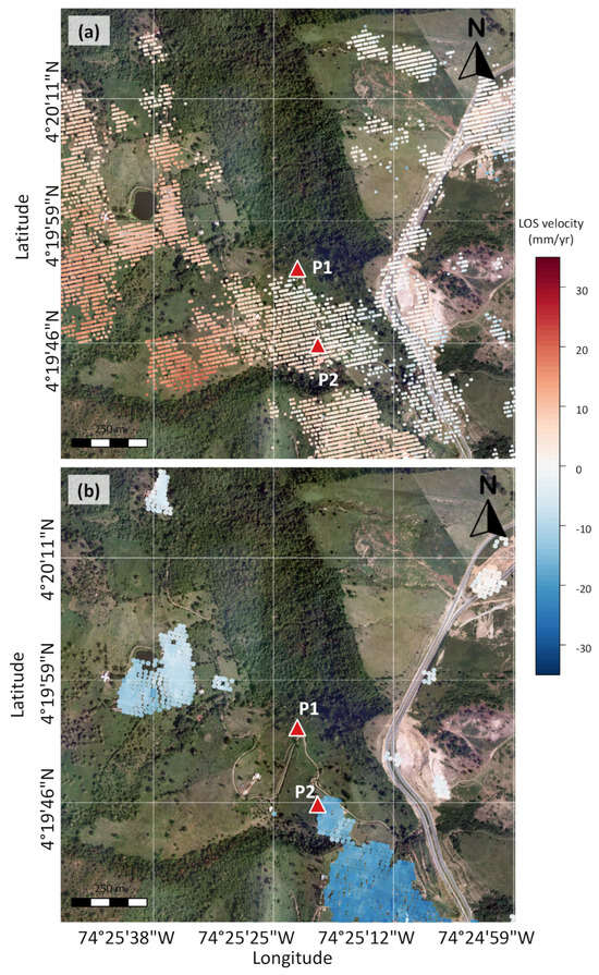
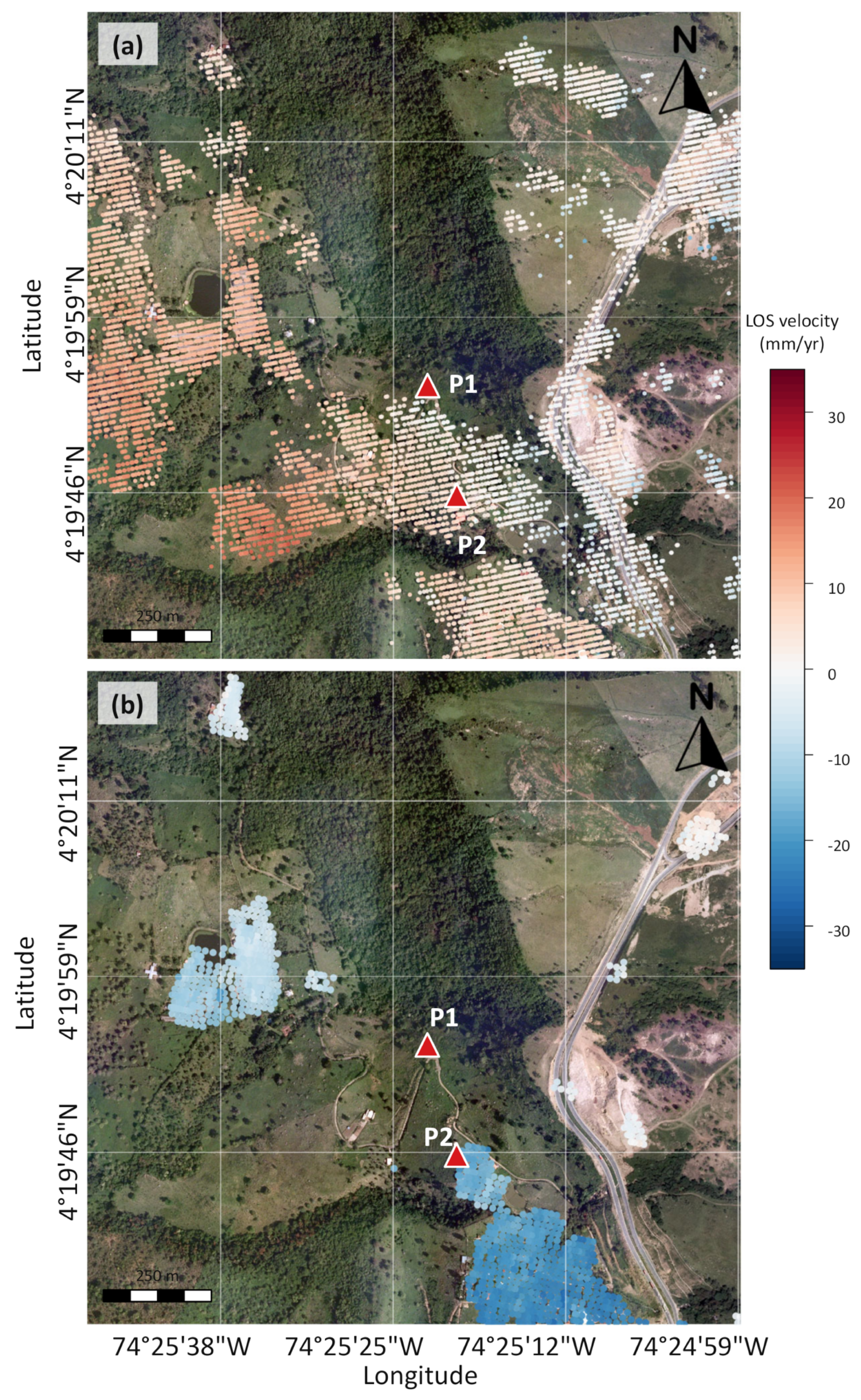
Figure 4 shows the InSAR results for San Antonio, Fusagasugá. Ascending and descending observations during 2020–2021 map average LOS deformation velocities around GNSS stations P1 and P2. The LOS velocities used for the P2 decomposition, +4.7 mm/year in ascending geometry and −17.8 mm/year in descending geometry, are the linear trends of the coherence-weighted local mean time series analyzed below. These series were calculated within 100 m of P2 using 326 ascending and 35 descending points with coherence $\ge 0.75$; the velocities therefore represent the local InSAR neighborhood rather than a single pixel or the four GNSS-epoch samples.

Figure 4. Average annual line-of-sight (LOS) deformation velocity in the San Antonio sector, Fusagasugá, derived from SBAS-InSAR results for 2020–2021. (a) Ascending-orbit result based on 7554 coherent scatterer points. (b) Descending-orbit result based on 1284 coherent scatterer points. Red triangles indicate GNSS stations P1 and P2.

At P1, reliable descending-orbit measurements were unavailable at the station because of low coherence. In the ascending-orbit dataset, nearby coherent scatterers located within approximately 50 m show an average LOS velocity of about −2 mm/year, which is close to the measurement resolution and should therefore be interpreted with caution.

The paired LOS velocities at P2 were inverted using Equation (1). With local incidence angles of $38.831°$ for the ascending geometry and $38.927°$ for the descending geometry, and assuming negligible northward motion, the solution is $d_E=-18.3$ mm/year (18.3 mm/year westward) and $d_U=-8.4$ mm/year (8.4 mm/year downward). The corresponding two-component magnitude is 20.1 mm/year. No decomposition was attempted at P1 because descending-orbit coverage was insufficient.

GNSS observations were carried out at stations P1 and P2 (Figure 1), in four different independent times for each site (Table 2), using the static technique, as already described. The national MAGNA-SIRGAS reference system and GRS80 ellipsoidal parameters (Geodetic Reference System, 1980) were used for data analysis. They were projected in the official origin for Colombia, called CTM-12 [31]. The coordinate and network adjustment was carried out with respect to the IGAC continuous observation stations (Table 2).

At P1 (Table 3), the 21/09/2021 east displacement of 793 mm is incompatible with the 0, 0, and −8 mm values at the other epochs. Its propagated uncertainty relative to the first epoch is 18.4 mm, obtained by combining the 14- and 12-mm epoch standard deviations in quadrature; the displacement is therefore 43.0 times its propagated standard deviation. It is not sustained in the subsequent campaign, when the displacement returns to −8 mm. Based on this extreme standardized deviation and its temporal inconsistency with the remaining observations, it is classified as a gross outlier, retained in Table 3 for transparency, and excluded from trend estimation and physical interpretation. The remaining P1 epochs do not support a resolved horizontal trend; only four campaigns are available.

Table 3. Coordinates and displacement components for GNSS station P1 in the MAGNA-SIRGAS reference frame. Displacements are referenced to the first observation (19/08/2021). All displacement and uncertainty values are expressed in millimeters (mm), whereas the coordinates are given in meters (m). N, E, and H denote northing, easting, and ellipsoidal height, respectively; $\mathrm{\Delta }N$, $\mathrm{\Delta }E$, and $\mathrm{\Delta }H$ denote displacements relative to the first observation. The reported ${\sigma }_N$, ${\sigma }_E$, and ${\sigma }_H$ values are the formal one-standard-deviation uncertainties of the adjusted coordinates at each epoch, not of the relative displacements.

Date	North	East	Height	$\mathbf{\Delta }\mathit{N}$	${\mathit{\sigma }}_{\mathit{N}}$	$\mathbf{\Delta }\mathit{E}$	${\mathit{\sigma }}_{\mathit{E}}$	$\mathbf{\Delta }\mathit{H}$	${\mathit{\sigma }}_{\mathit{H}}$
19/08/2021	2,036,777.476	4,842,161.569	1326.568	0	9	0	12	0	30
26/08/2021	2,036,777.471	4,842,161.569	1326.453	−5	6	0	7	−115	22
21/09/2021	2,036,777.470	4,842,162.362	1326.495	−6	12	793	14	−73	37
23/11/2021	2,036,777.472	4,842,161.561	1326.487	−4	9	−8	12	−81	31

Station P2 is located only 260 m from P1 (Figure 4), yet its four campaign solutions differ substantially (Table 4). At the final epoch, P2 reaches $\mathrm{\Delta }H=242$ mm, $\mathrm{\Delta }E=-20$ mm, and $\mathrm{\Delta }N=15$ mm relative to the first observation. The large vertical change dominates the GNSS LOS projection and is not reproduced by the local InSAR time series, as quantified below. Accordingly, these sparse GNSS results are treated as complementary point measurements rather than evidence that validates the spatially averaged InSAR signal.

Table 4. Coordinates and displacement components for GNSS station P2 in the MAGNA-SIRGAS reference frame. Displacements are referenced to the first observation (29/06/2021). All displacement and uncertainty values are expressed in millimeters (mm), whereas the coordinates are given in meters (m). N, E, and H denote northing, easting, and ellipsoidal height, respectively; $\mathrm{\Delta }N$, $\mathrm{\Delta }E$, and $\mathrm{\Delta }H$ denote displacements relative to the first observation. The reported ${\sigma }_N$, ${\sigma }_E$, and ${\sigma }_H$ values are the formal one-standard-deviation uncertainties of the adjusted coordinates at each epoch, not of the relative displacements.

Date	North	East	Height	$\mathbf{\Delta }\mathit{N}$	${\mathit{\sigma }}_{\mathit{N}}$	$\mathbf{\Delta }\mathit{E}$	${\mathit{\sigma }}_{\mathit{E}}$	$\mathbf{\Delta }\mathit{H}$	${\mathit{\sigma }}_{\mathit{H}}$
29/06/2021	2,036,529.629	4,842,228.802	1363.721	0	15	0	16	0	47
16/08/2021	2,036,529.633	4,842,228.793	1363.755	4	9	−9	11	34	33
22/09/2021	2,036,529.633	4,842,228.783	1363.782	4	1	−19	1	61	2
24/11/2021	2,036,529.644	4,842,228.782	1363.963	15	9	−20	11	242	29

The continuous reference stations used for GNSS adjustment belong to the Colombian National Geodetic Network and were assumed stable in the campaign solution. This network reference does not by itself diagnose receiver processing, antenna setup, or local monument behavior and therefore cannot establish that the P2 changes are true ground deformation.

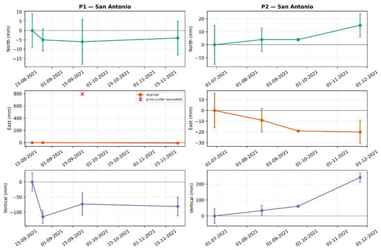
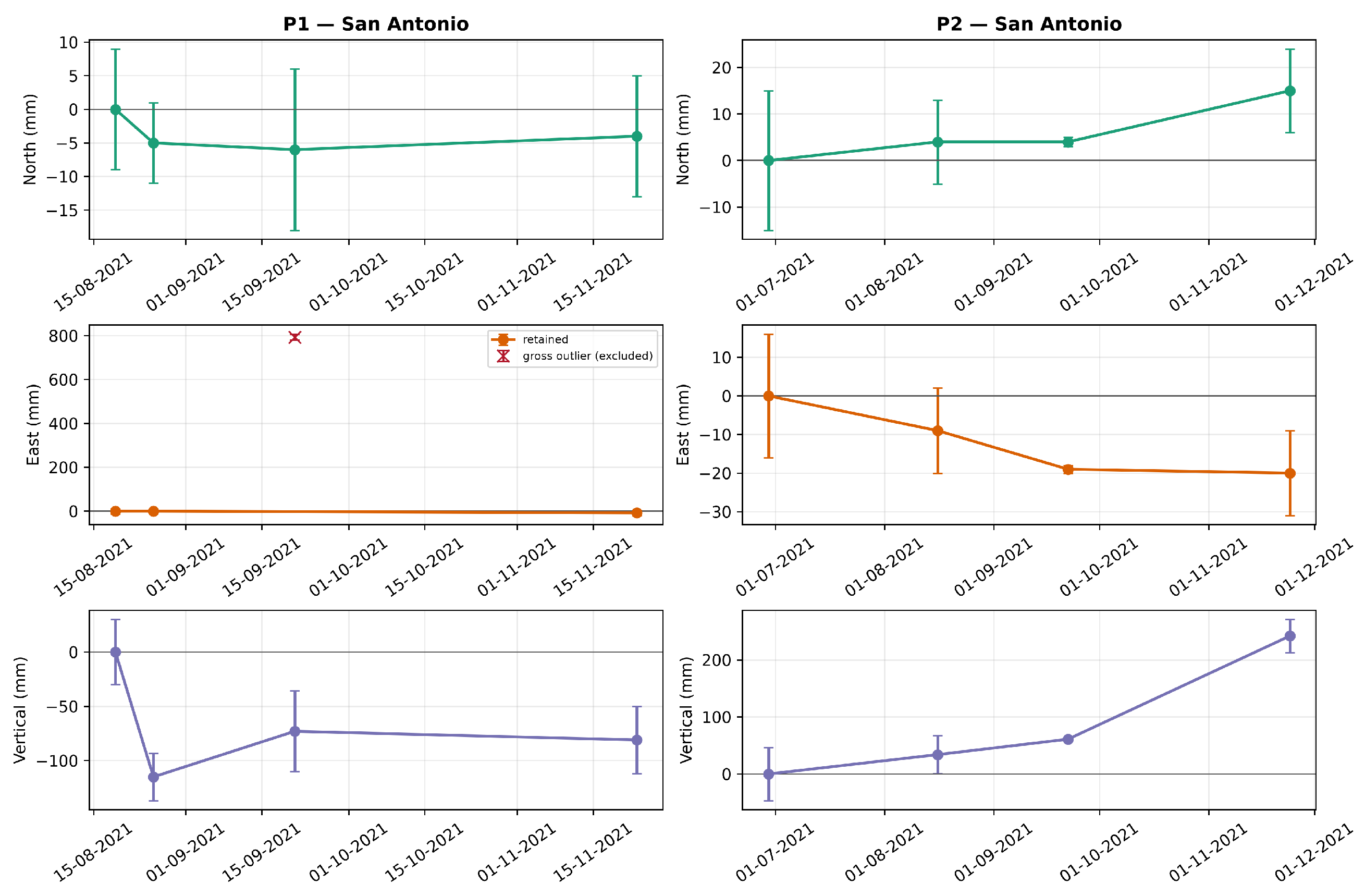
Figure 5 displays the component time series and formal uncertainties. P1 shows only small north and east changes after exclusion of the 793-mm gross outlier, while its vertical component varies between 0 and −115 mm. P2 reaches 15 mm north, −20 mm east, and 242 mm up at the last campaign. Because the series contain only four epochs over three to five months, the apparent component changes should not be extrapolated as long-term velocities.

Figure 5. GNSS displacement time series for P1 (left) and P2 (right). Rows show north, east, and vertical components. Error bars show the reported one-standard-deviation coordinate-solution uncertainties at each epoch. The P1 east value of 793 mm is marked as a gross outlier and is not connected to the retained observations or used in interpretation.

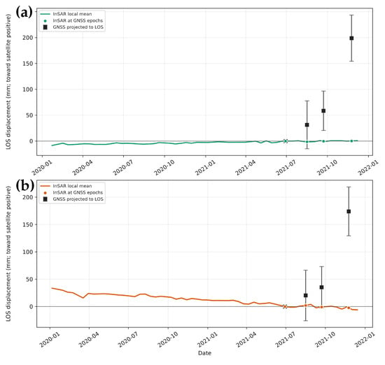
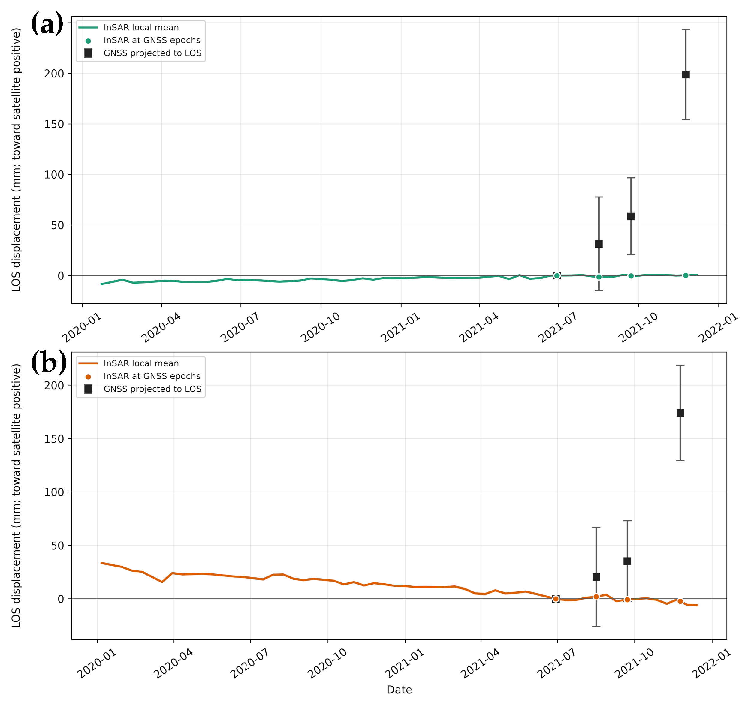
Applying Equation (2), the P2 GNSS displacement vectors were projected into both satellite LOS directions (Figure 6), retaining the north component and using the positive-toward-satellite sign convention defined above. All four P2 epochs, together with the corresponding P3 and P4 comparisons, are reported in Supplementary Table S9 and Dataset S2.

Figure 6. P2 ascending (a) and descending (b) LOS comparisons. InSAR curves are coherence-weighted means of 326 ascending and 35 descending points with coherence $\ge 0.75$ within 100 m of P2; their full-period linear trends are +4.7 and −17.8 mm/year, respectively. Shaded bands are weighted spatial standard errors. Squares are GNSS displacements projected with Equation (2), with propagated $1\sigma$ error bars. Each comparison is independently referenced to 29/06/2021.

The GNSS and InSAR series do not agree quantitatively. At the final epoch, the projected GNSS displacements are +198.9 ± 44.7 mm (ascending) and +174.1 ± 44.6 mm (descending), whereas the corresponding local InSAR estimates are +0.3 and −2.3 mm. Descriptive four-epoch RMSE values are 104.9 mm (ascending) and 90.5 mm (descending). The discrepancy is therefore reported directly rather than attributed to a single unverified cause or used as validation. Plausible contributors include point-versus-area sampling, GNSS monument or campaign errors, unresolved phase behavior, and the unverified InSAR reference datum; the available records cannot discriminate among them.

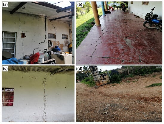
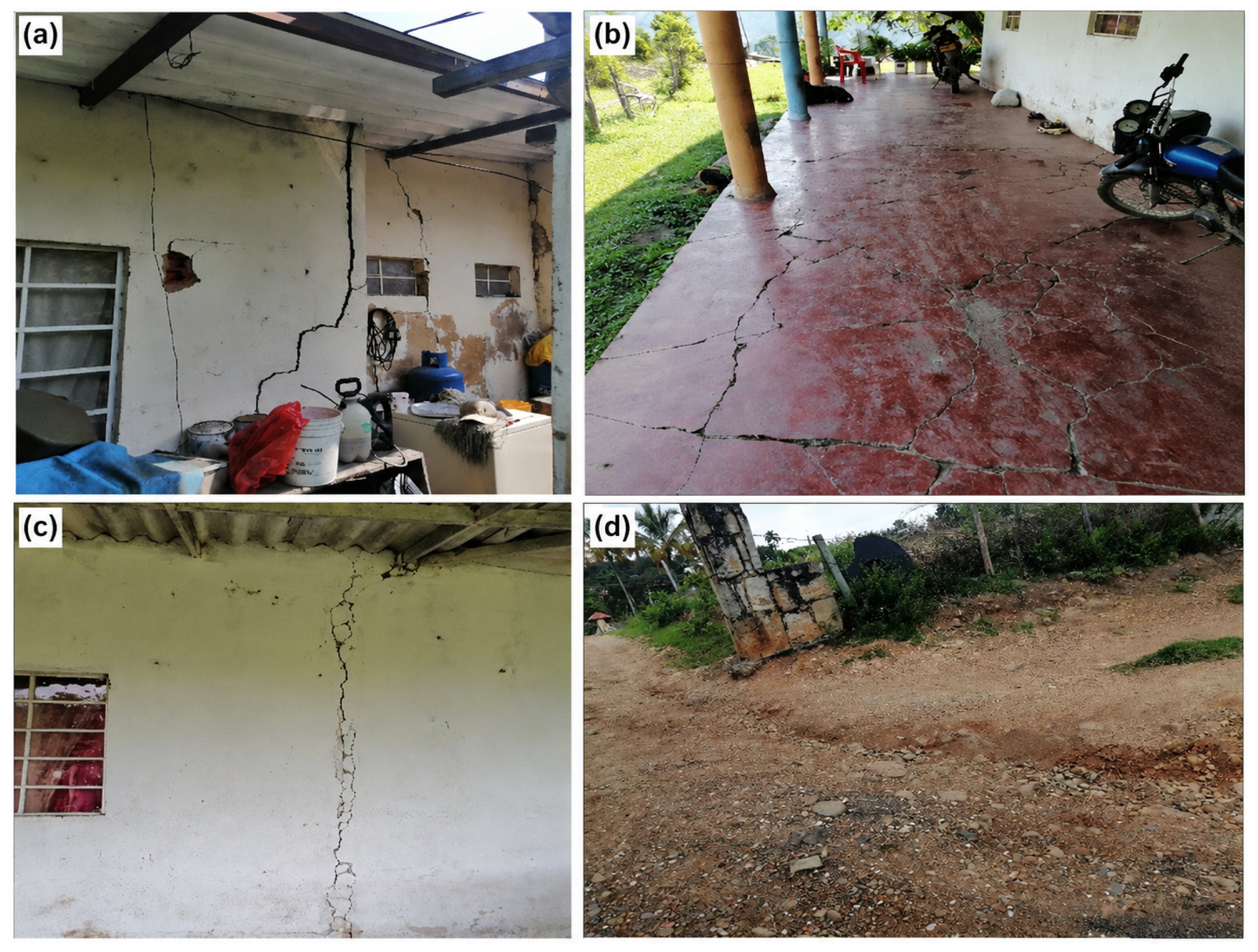
Field inspection near P1 and P2 documented cracks and fractures in roads and buildings (Figure 7). These observations establish the presence of structural damage, but they are not direct proof of the displacement mechanism, timing, or correspondence with an InSAR pixel. Possible causes include ground movement, construction practice, material deterioration, drainage, and other local effects. The photographs are therefore contextual observations that motivate follow-up geotechnical investigation.

Figure 7. Structural damage documented near P1 and P2 in San Antonio: (a) wall cracking; (b) fractures on a porch slab; (c) a vertical exterior-wall crack; and (d) cracking and deformation of an access road. The photographs provide field context but do not establish cause or direct correspondence with the InSAR signal.

4.2. San Luis Bajo Sector, Municipality of Silvania, Cundinamarca

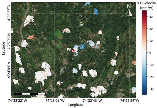
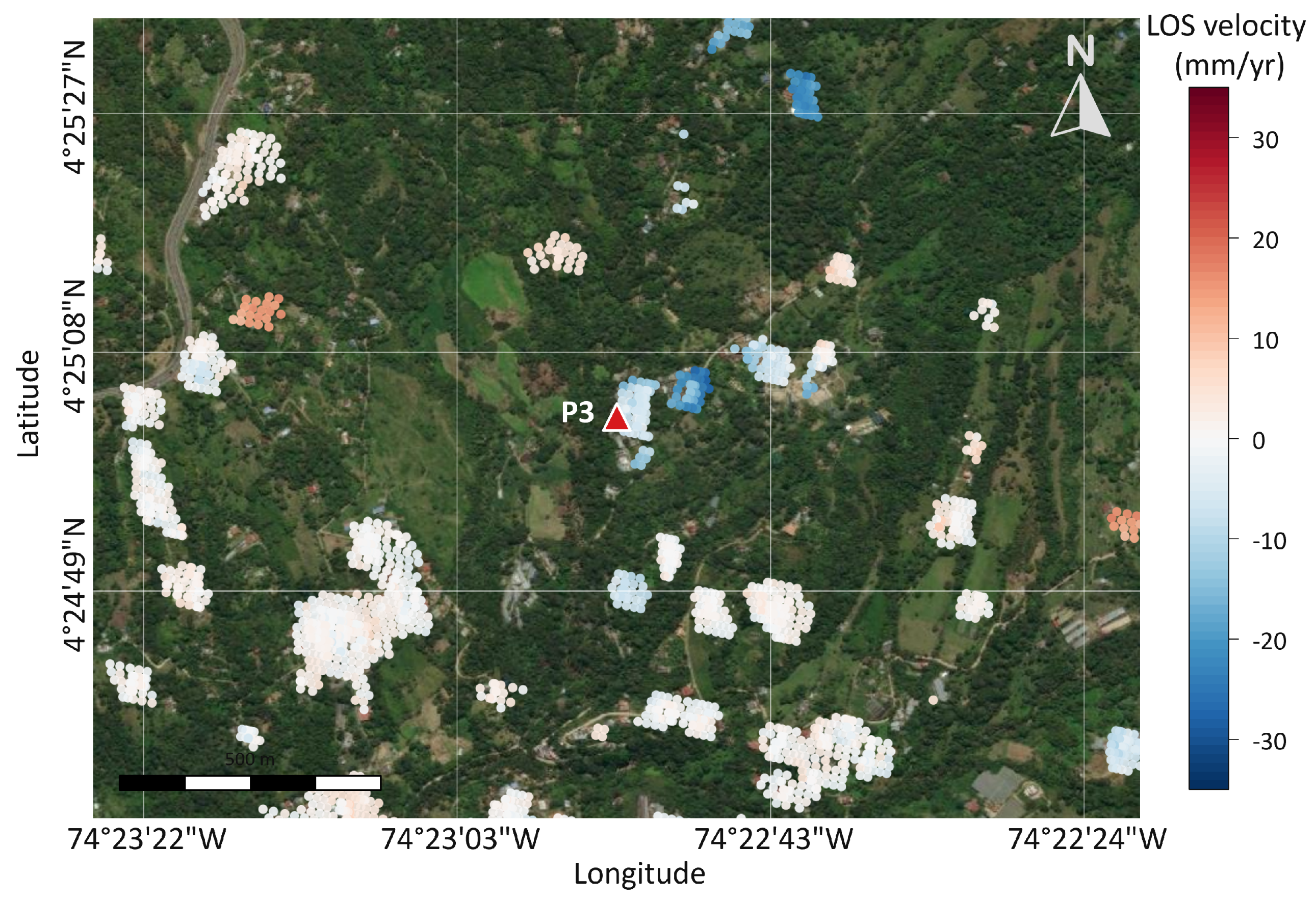
Figure 8 shows the distribution of 2640 coherent measurement points and the average LOS deformation velocity derived from descending-orbit SBAS-InSAR data in the San Luis Bajo sector, Silvania. In this area, only the descending-orbit dataset provided a reliable deformation solution. The density of coherent measurement points around GNSS station P3 was relatively low, limiting the spatial sampling of the deformation field. Although ascending scenes were also processed, lower measurement-point density and coherence prevented a reliable ascending-orbit deformation solution.

Figure 8. Average LOS deformation velocity map for San Luis Bajo, Silvania, derived from descending-orbit SBAS-InSAR data for 06/01/2020–14/12/2021. The map includes 2640 measurement points; negative LOS velocities indicate motion away from the satellite. The red triangle indicates P3.

Equation (1) could not be applied in the area corresponding to station P3 because the ascending-orbit data did not provide sufficient coherent coverage around the station. Consequently, only the descending-orbit LOS deformation could be interpreted for this sector, and the separation of east–west and vertical components was not attempted.

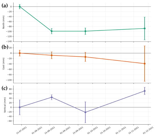
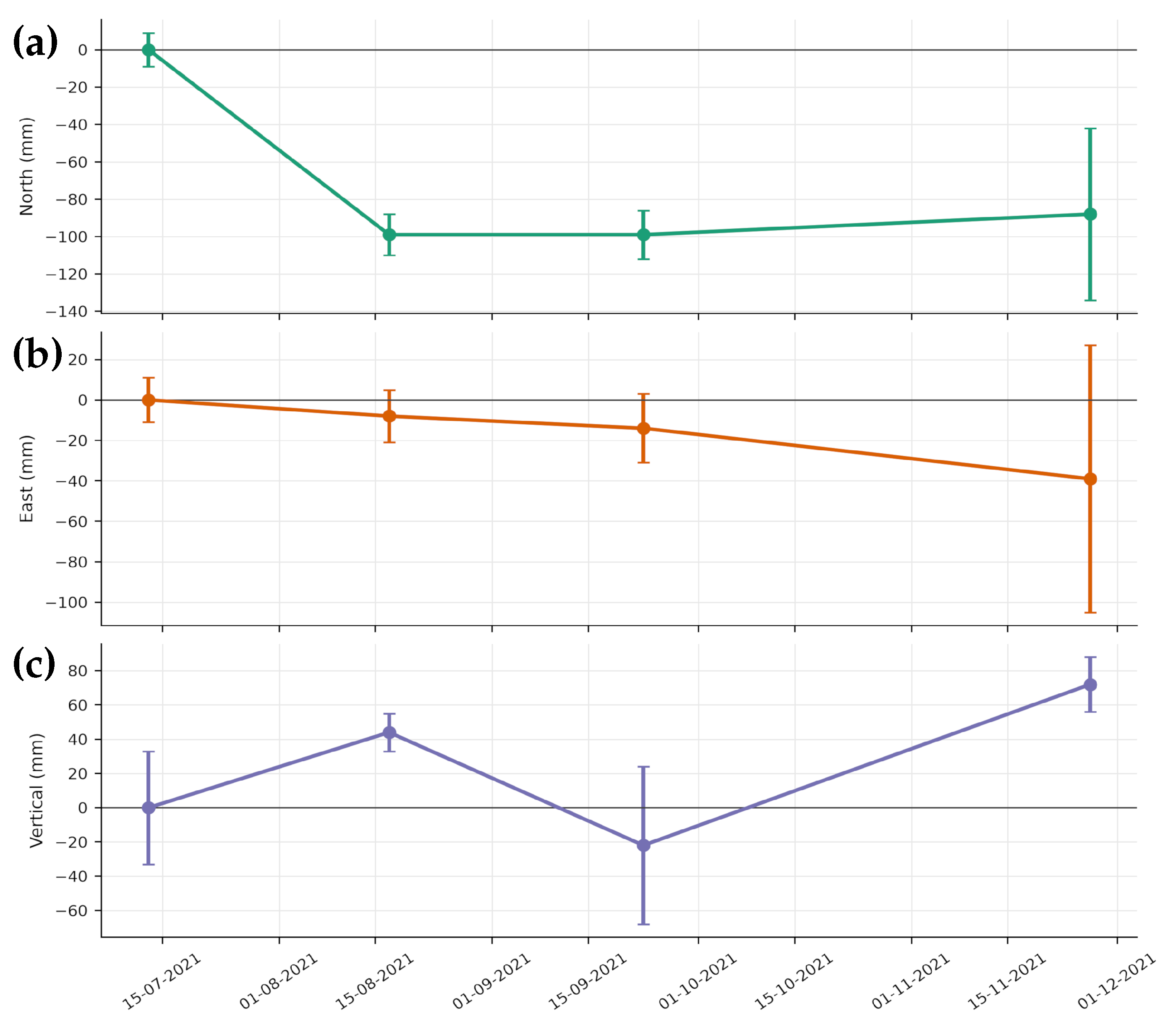
At P3, four campaign observations are presented in Table 5 and Figure 9. The coordinate differences suggest southwestward motion and alternating vertical changes, but several uncertainties are of the same order as the displacements. The series is therefore insufficient for a precise trajectory or long-term velocity.

Table 5. Coordinates and displacement components for GNSS station P3 in the MAGNA-SIRGAS reference frame. Displacements are referenced to the first observation (13/07/2021). All displacement and uncertainty values are expressed in millimeters (mm), whereas the coordinates are given in meters (m). N, E, and H denote northing, easting, and ellipsoidal height, respectively; $\mathrm{\Delta }N$, $\mathrm{\Delta }E$, and $\mathrm{\Delta }H$ denote displacements relative to the first observation. The reported ${\sigma }_N$, ${\sigma }_E$, and ${\sigma }_H$ values are the formal one-standard-deviation uncertainties of the adjusted coordinates at each epoch, not of the relative displacements.

Date	North	East	Height	$\mathbf{\Delta }\mathit{N}$	${\mathit{\sigma }}_{\mathit{N}}$	$\mathbf{\Delta }\mathit{E}$	${\mathit{\sigma }}_{\mathit{E}}$	$\mathbf{\Delta }\mathit{H}$	${\mathit{\sigma }}_{\mathit{H}}$
13/07/2021	2,046,264.892	4,846,790.409	1521.936	0	9	0	11	0	33
17/08/2021	2,046,264.793	4,846,790.401	1521.980	−99	11	−8	13	44	11
23/09/2021	2,046,264.793	4,846,790.395	1521.914	−99	13	−14	17	−22	46
27/11/2021	2,046,264.804	4,846,790.370	1522.008	−88	46	−39	66	72	16

Figure 9. GNSS displacement time series for station P3 (San Luis Bajo): (a) north, (b) east, and (c) vertical components. Error bars represent the corresponding $1\sigma$ uncertainties.

At the last P3 observation, the displacements relative to 13/07/2021 were $\mathrm{\Delta }N=-88$ mm, $\mathrm{\Delta }E=-39$ mm, and $\mathrm{\Delta }H=72$ mm. The corresponding formal coordinate-solution standard deviations at this epoch were ${\sigma }_N=46$ mm, ${\sigma }_E=66$ mm, and ${\sigma }_H=16$ mm (Table 5). The horizontal direction is nominally southwest, but the large east uncertainty and sparse temporal sampling require caution. The campaign solutions provide complementary measurements in the national geodetic frame, not an independent validation of the InSAR series.

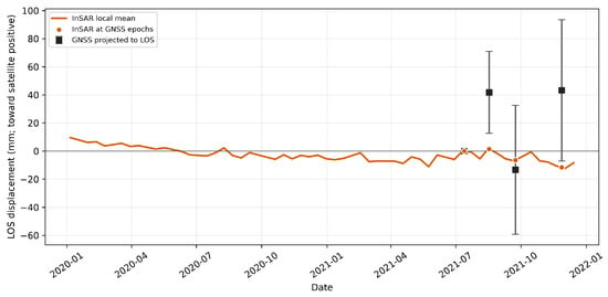
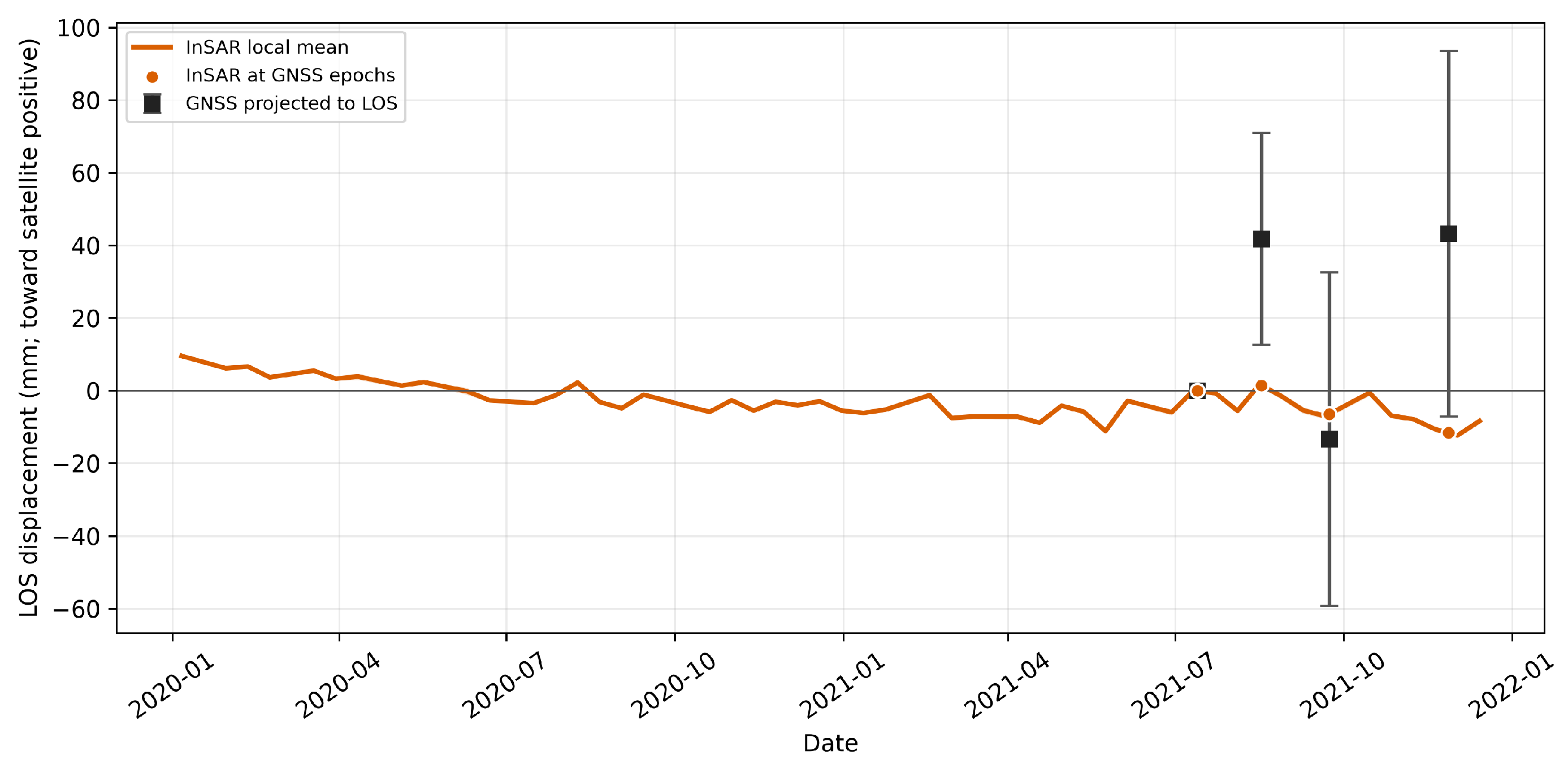
Equation (2) projects the P3 GNSS vectors into descending LOS. The local InSAR series is a coherence-weighted mean of 40 points within 100 m, referenced to the first campaign.

Figure 10 shows no consistent epoch-by-epoch agreement. Projected GNSS LOS values after the reference epoch are +41.9 ± 29.1, −13.2 ± 45.9, and +43.3 ± 50.4 mm; interpolated InSAR values are +1.5, −6.5, and −11.6 mm. The descriptive four-epoch RMSE is 34.2 mm. Because the uncertainty intervals are broad and only four GNSS epochs are available, this comparison neither confirms nor falsifies the local InSAR trend.

Figure 10. Descending LOS comparison at P3. The InSAR curve is a coherence-weighted mean of 40 points within 100 m; the band is its weighted spatial standard error. Squares are GNSS displacements projected to LOS with propagated $1\sigma$ uncertainty. Both series are referenced to 13/07/2021.

A field inspection around P3 documented fissures and cracks in nearby buildings (Figure 11). The sector is approximately 900 m from the mapped Fusagasugá syncline (Figure 1 and Figure 2). This proximity and the reported history of instability provide geological context, but neither the cracks nor proximity to a mapped structure demonstrates causation or validates a particular geodetic time series.

Figure 11. Structural damage observed near P3 in San Luis Bajo: (a) exterior-wall cracking and the GNSS receiver; (b) porch-slab fractures; (c) a major wall crack; and (d) extensive exterior-wall cracking. These observations document damage but do not establish its cause or timing.

4.3. El Bermejal Sector, Municipality of Fusagasugá, Cundinamarca

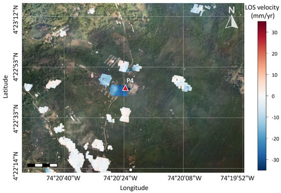
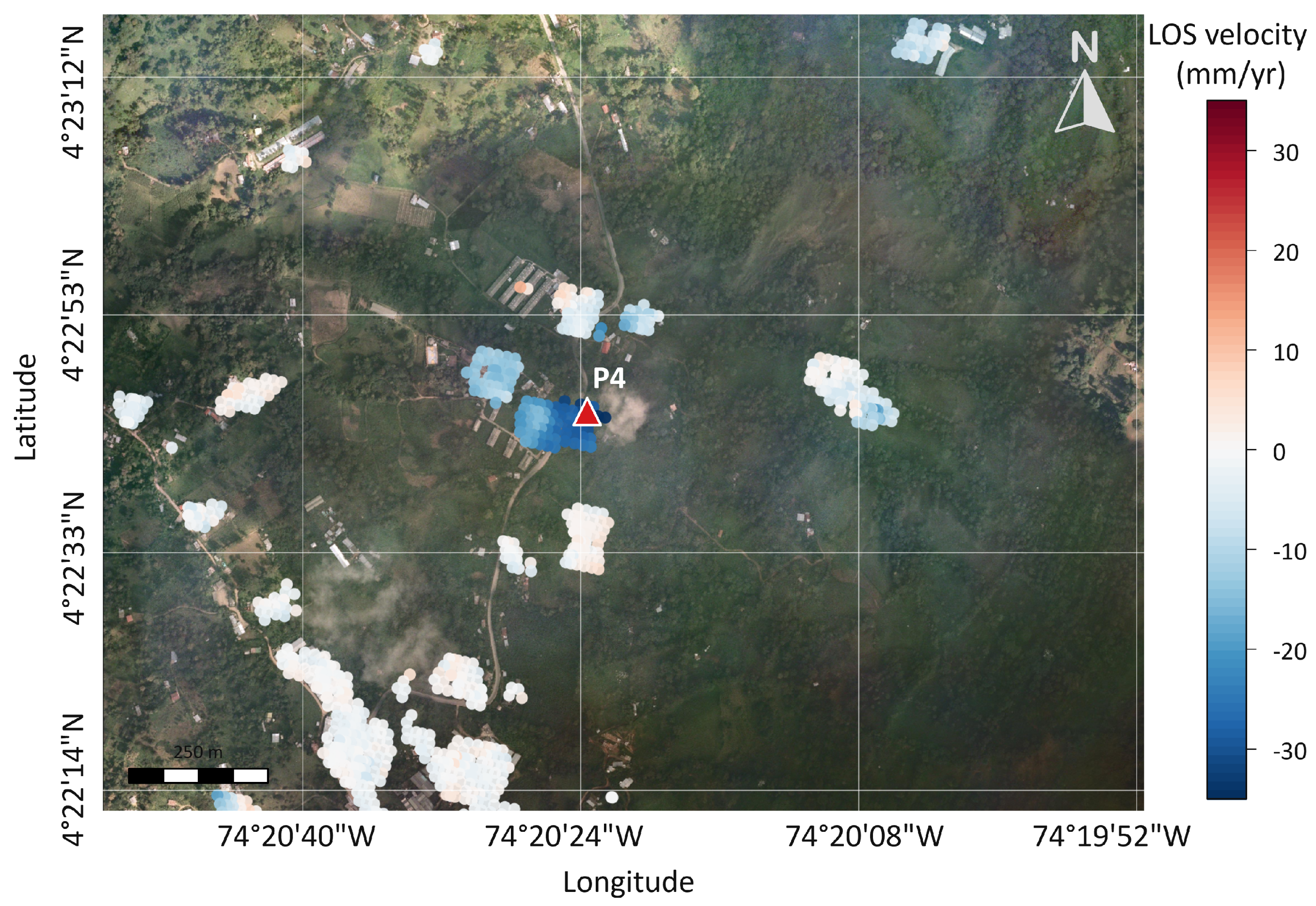
Figure 12 shows the InSAR results in the area connecting the population centers of Fusagasugá and La Aguadita. The analysis, carried out in descending mode, covers the period from 6 January 2020, to 14 December 2021. The results show LOS velocities reaching approximately −31 mm/year, indicating motion away from the satellite during this period.

Figure 12. Average LOS deformation velocity map for El Bermejal, Fusagasugá, derived from descending-orbit SBAS-InSAR data for 06/01/2020–14/12/2021. The map includes 1122 measurement points; negative LOS velocities indicate motion away from the satellite. The red triangle indicates P4.

The ascending-orbit data did not provide sufficient coherent scatterer coverage for this sector; Equation (1) could not be used to decompose the LOS displacement into east–west and vertical components. This limitation prevented a complete vector decomposition of the deformation field and reduced the analysis to the descending-orbit LOS component.

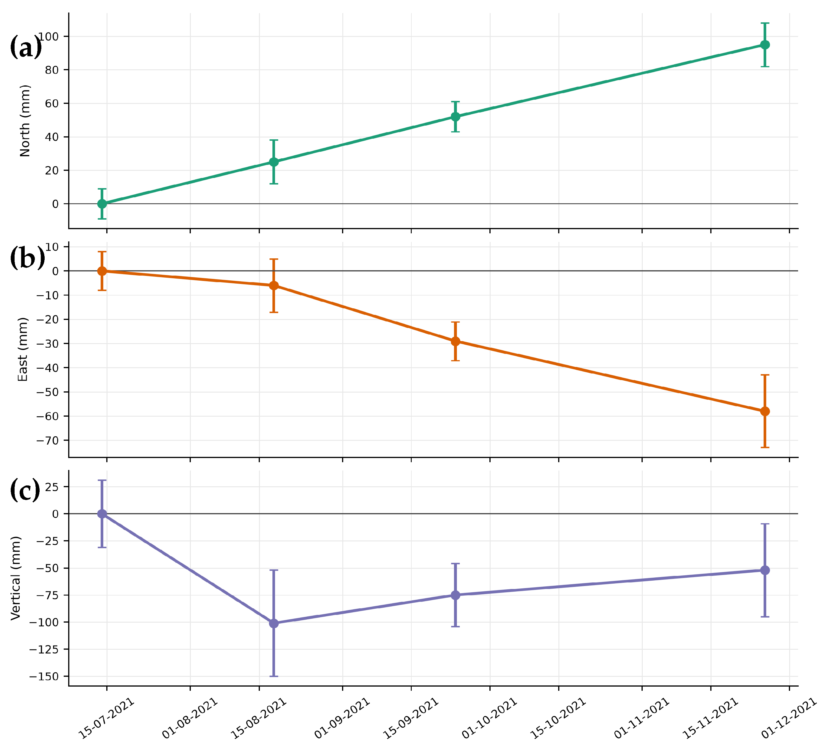
At P4 (Table 6), the final solution gives $\mathrm{\Delta }N=95$ mm, $\mathrm{\Delta }E=-58$ mm, and $\mathrm{\Delta }H=-52$ mm relative to 14/07/2021. The corresponding formal coordinate-solution standard deviations at the final epoch were ${\sigma }_N=13$ mm, ${\sigma }_E=15$ mm, and ${\sigma }_H=43$ mm. The largest negative vertical displacement was −101 mm on 2021/08/18, for which the epoch coordinate-solution standard deviation was ${\sigma }_H=49$ mm. These four campaign results indicate coordinate changes but do not identify their cause.

Table 6. Coordinates and displacement components for GNSS station P4 in the MAGNA-SIRGAS reference frame. Displacements are referenced to the first observation (14/07/2021). All displacement and uncertainty values are expressed in millimeters (mm), whereas the coordinates are given in meters (m). The reported ${\sigma }_N$, ${\sigma }_E$, and ${\sigma }_H$ values are the formal one-standard-deviation uncertainties of the adjusted coordinates at each epoch, not of the relative displacements.

Date	North	East	Height	$\mathbf{\Delta }\mathit{N}$	${\mathit{\sigma }}_{\mathit{N}}$	$\mathbf{\Delta }\mathit{E}$	${\mathit{\sigma }}_{\mathit{E}}$	$\mathbf{\Delta }\mathit{H}$	${\mathit{\sigma }}_{\mathit{H}}$
14/07/2021	2,042,018.689	4,851,372.436	1843.048	0	9	0	8	0	31
18/08/2021	2,042,018.714	4,851,372.430	1842.947	25	13	−6	11	−101	49
24/09/2021	2,042,018.741	4,851,372.407	1842.973	52	9	−29	8	−75	29
26/11/2021	2,042,018.784	4,851,372.378	1842.996	95	13	−58	15	−52	43

Figure 13 shows the three-component GNSS displacement series at P4. By the final epoch, P4 reaches $\mathrm{\Delta }N=95$ mm, $\mathrm{\Delta }E=-58$ mm, and $\mathrm{\Delta }H=-52$ mm relative to the first campaign. The vertical component has larger formal uncertainties than the horizontal components, with ${\sigma }_H$ reaching 49 mm.

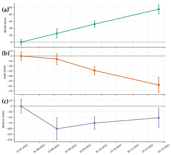
Figure 13. GNSS displacement time series at P4 in the El Bermejal sector, Fusagasugá, showing the north–south (a), east–west (b), and vertical (c) components during the observation period.

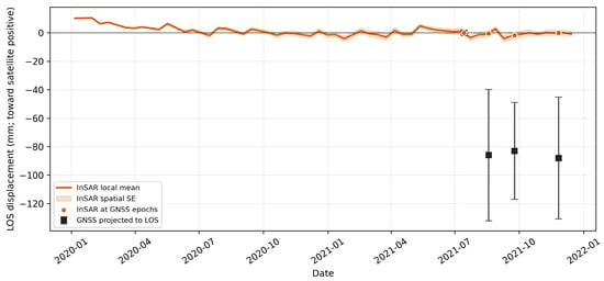
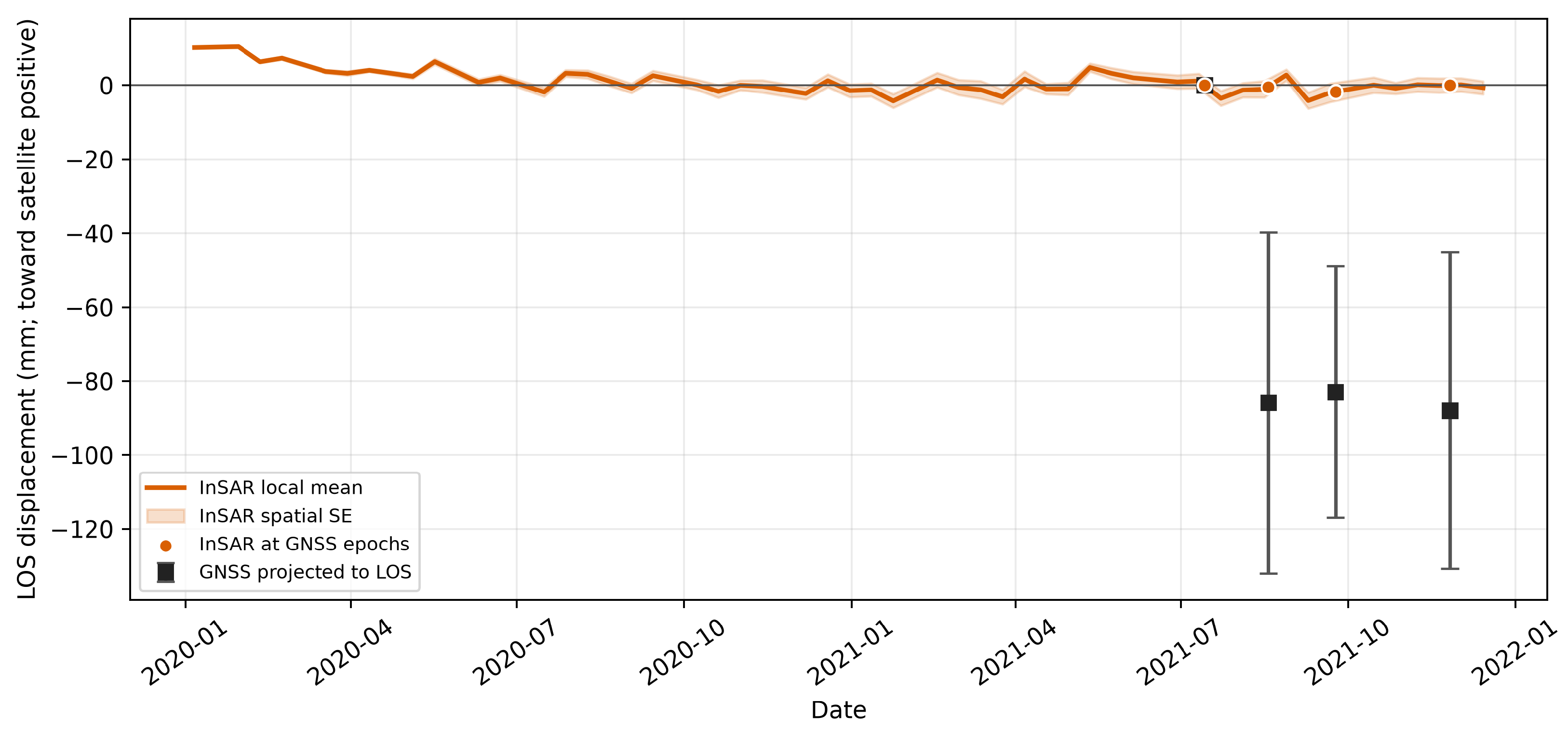
Applying Equation (2), the P4 GNSS series gives descending LOS values of −85.9 ± 46.2, −82.9 ± 34.0, and −88.0 ± 42.8 mm after the reference epoch. The corresponding coherence-weighted InSAR values from 53 points within 260 m are −0.4, −1.7, and 0.0 mm (Figure 14). The descriptive four-epoch RMSE is 73.6 mm. The large magnitude discrepancy precludes quantitative validation; resolving it will require repeat GNSS occupations and checks of the monument and reference realization.

Figure 14. Descending LOS comparison at P4. The InSAR curve is a coherence-weighted mean of 53 points within 260 m; the band is its weighted spatial standard error. Squares are GNSS displacements projected to LOS with propagated $1\sigma$ uncertainty. Both series are referenced to 14/07/2021.

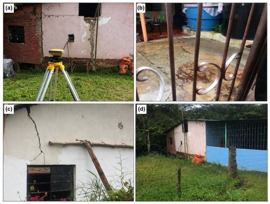
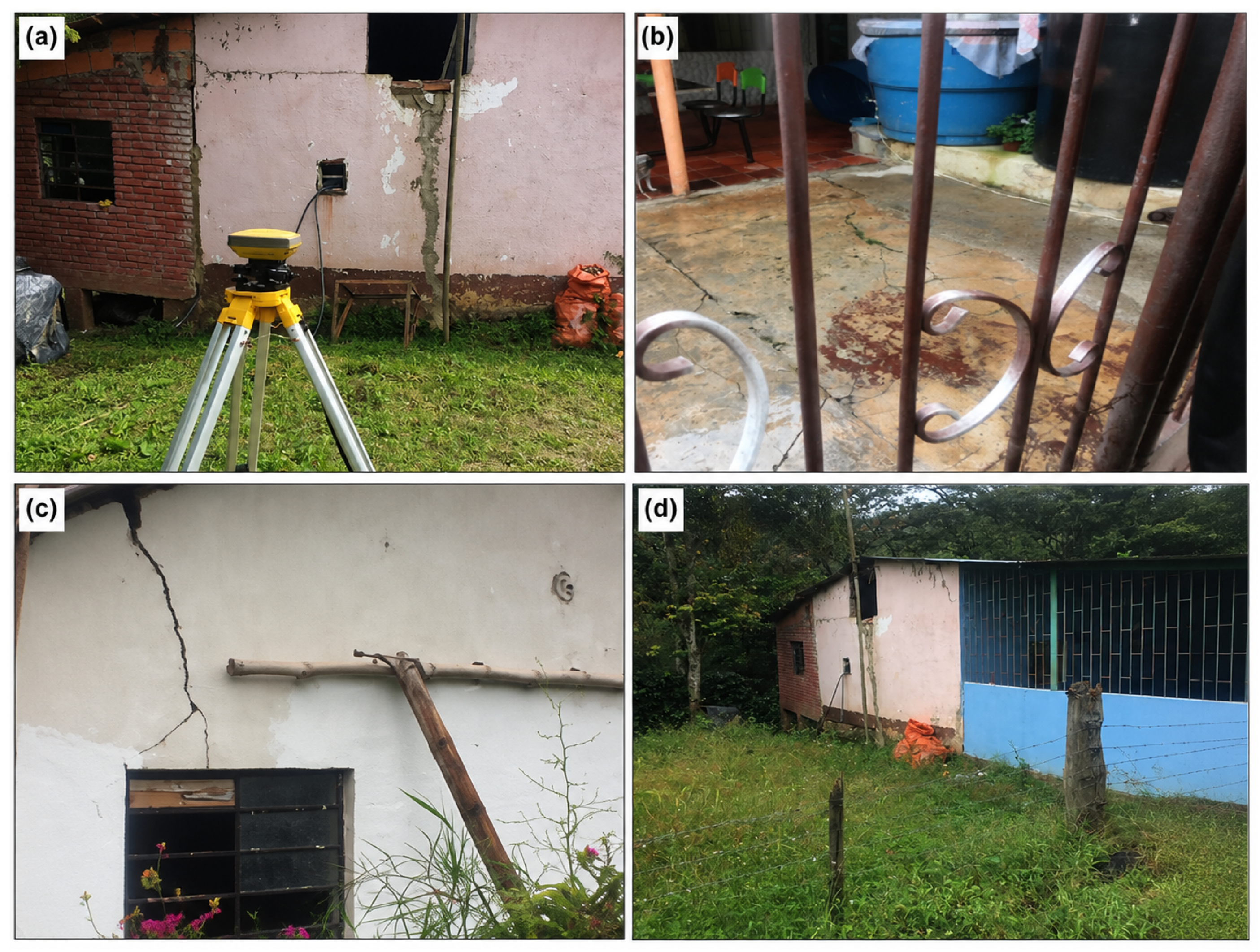
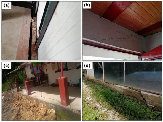
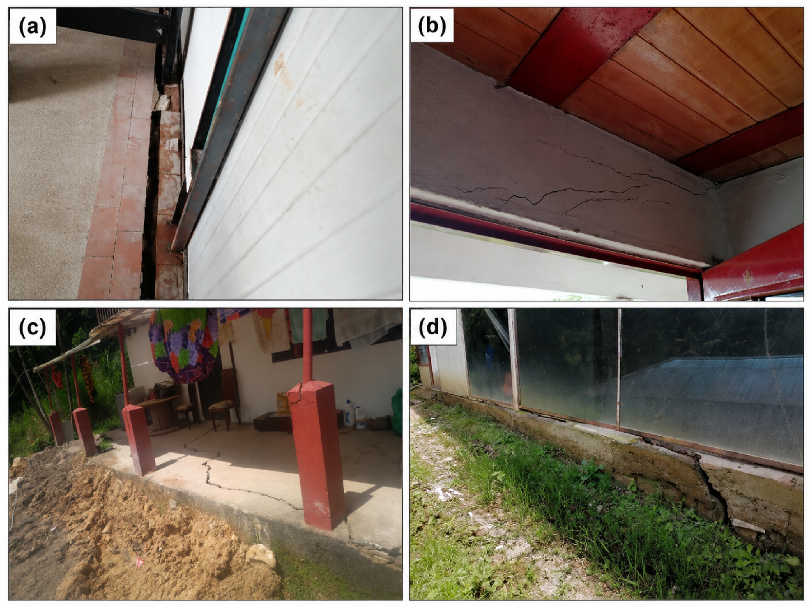
Near P4, residents reported damage to roads and buildings, and field visits documented fissures and breaks in walls, floors, and foundations (Figure 15). The sector is approximately 800 m from the mapped Fusagasugá fault. These observations motivate detailed engineering-geological investigation, but neither fault proximity nor visible cracks establishes the deformation mechanism or a direct relationship with the InSAR measurements.

Figure 15. Damage documented in El Bermejal along the Fusagasugá–La Aguadita road: (a) separation between a floor slab and wall; (b) upper-wall cracking; (c) cracks in a porch slab and structural elements; and (d) foundation cracking at an agro-industrial greenhouse. The photographs document damage but do not establish cause or correspondence with an InSAR pixel.

5. Discussion

5.1. Spatial Deformation Patterns and Viewing-Geometry Constraints

The Sentinel-1 analysis identifies spatially coherent LOS deformation in San Antonio, San Luis Bajo, and El Bermejal despite heterogeneous rural coverage. San Antonio is the only sector with sufficient paired ascending- and descending-orbit measurements for a two-component solution near P2. Under the assumption of negligible north–south motion, the representative velocities yield $d_E=-18.3$ mm/year (18.3 mm/year westward) and $d_U=-8.4$ mm/year (8.4 mm/year downward). This solution represents the east–west and vertical components of the average InSAR velocity field and should not be interpreted as a complete three-dimensional displacement vector. San Luis Bajo and El Bermejal are interpreted only in descending LOS because ascending-orbit coherent coverage is insufficient. These geometry-dependent differences limit direct comparison of motion components among the three sectors.

5.2. GNSS–InSAR Comparison and Measurement Uncertainty

The GNSS–InSAR comparison reveals substantial inconsistencies. At P2, the absolute differences at the final epoch are approximately 199 and 176 mm for the ascending and descending LOS projections, respectively, whereas the corresponding difference at P4 is approximately 88 mm. At P3, the projected GNSS observations have broad uncertainties and mixed residual signs. GNSS samples a single monument during four approximately six-hour occupations, whereas the local InSAR curves represent spatial averages of 35–326 coherent measurement points within 100 m at P2, 40 points within 100 m at P3, and 53 points within 260 m at P4. These differences in spatial and temporal support may contribute to the observed discrepancies [40], but they do not uniquely explain them. Reference-datum uncertainty, campaign or monument problems, unresolved phase behavior, and genuinely localized deformation remain possible contributors. Accordingly, campaign GNSS is treated here as complementary point-scale evidence rather than as independent validation of the InSAR time series.

The 793-mm eastward displacement reported at P1 further illustrates the limitations of the campaign GNSS dataset. This value is 43.0 times its propagated standard deviation relative to the first epoch and is absent at the subsequent epoch; it is therefore treated as a gross outlier and excluded from kinematic interpretation. Repeat occupations, reprocessing of the raw GNSS observations, stable monuments or corner reflectors, and a documented common reference framework would be required for a more rigorous GNSS–InSAR validation.

5.3. Hydrometeorological and Geological Context

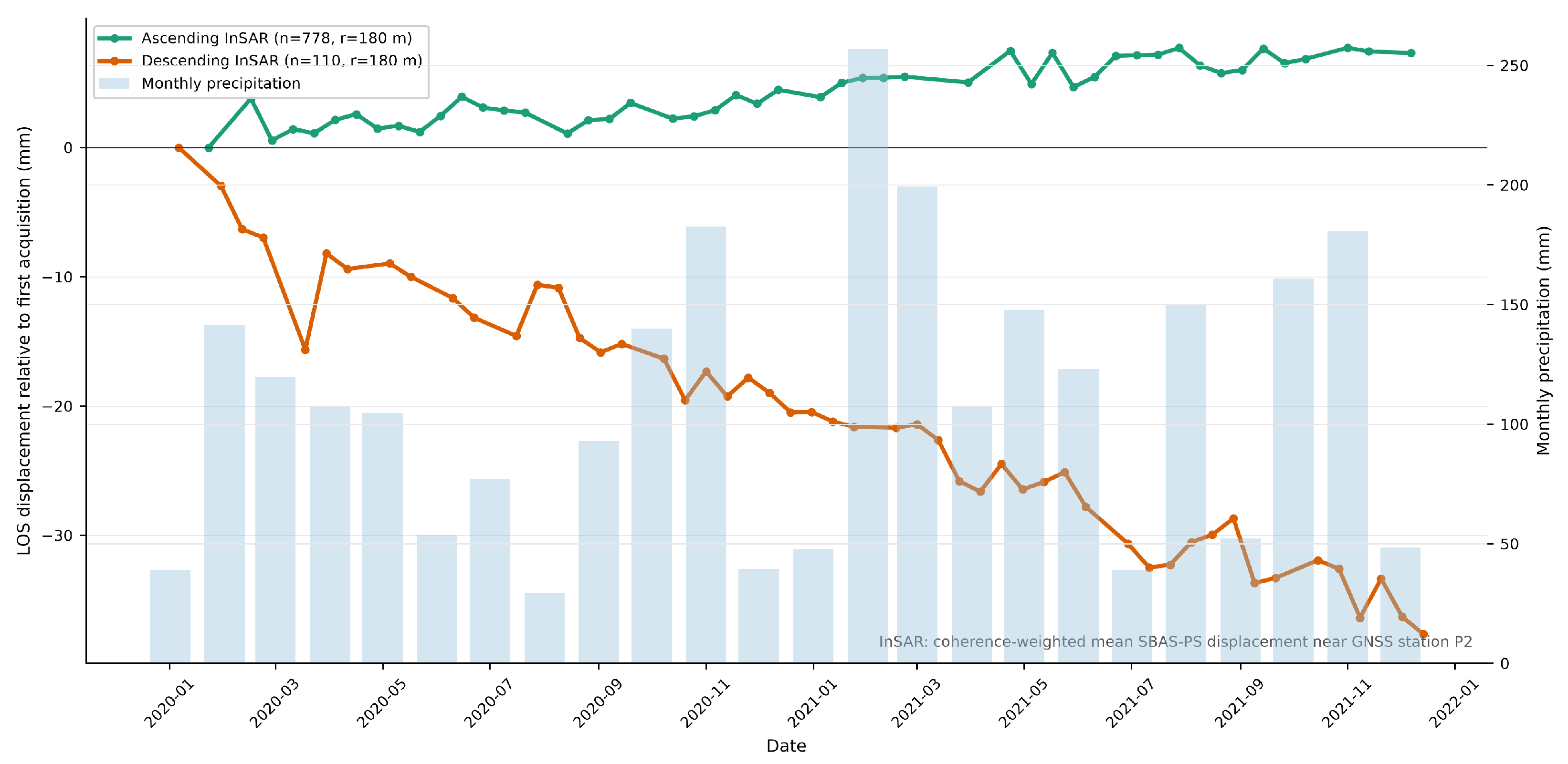
Monthly rainfall totals from CAR station 2119514 (UNIV. FUSAGASUGA), provided in Table S10 of the Supplementary Materials, were used to provide hydrometeorological context for the 2020–2021 InSAR observation period (Figure 16). Because instrument metadata, original quality-control information, and measurement uncertainties were not available, the rainfall series is used only descriptively, and no formal rainfall–deformation relationship is inferred.

Figure 16. Ascending and descending InSAR LOS displacement series for the San Antonio/P2 neighborhood and monthly accumulated rainfall for January 2020–December 2021. Rainfall values are monthly totals from CAR station 2119514, UNIV. FUSAGASUGA; no monthly value is missing in the supplied 24-month series. The overlay is descriptive and does not test correlation or causality.

Although hydrometeorological forcing is important in many mass-movement processes [41,42], visual correspondence between monthly rainfall and an InSAR displacement curve does not demonstrate correlation or triggering. Likewise, mapped faults and observed structural damage provide geological and field context but do not establish causal attribution. Testing these hypotheses would require event-scale precipitation, soil-moisture or pore-pressure observations, slope-unit kinematics, detailed field mapping, and geotechnical measurements.

5.4. Limitations and Implications for Regional Monitoring

The principal limitations of this study include the two-year Sentinel-1 observation interval, viewing-geometry and coherence gaps, only four GNSS campaigns per site, unresolved GNSS–InSAR discrepancies, the P1 gross outlier, the absence of an independent InSAR reference-stability test and complete pair-by-pair quality-control records, and incomplete rainfall metadata. These limitations constrain both the kinematic interpretation and attribution of the mapped deformation signals.

The deformation maps are therefore best used as screening products for prioritizing follow-up monitoring and field investigation. They cannot be converted directly into landslide susceptibility, hazard, risk, or warning classes [43,44]. A formal susceptibility assessment would require a landslide inventory, relevant conditioning factors, and model calibration and validation, whereas operational early warning would additionally require near-real-time observations and calibrated decision thresholds. Priority future work includes reprocessing the raw GNSS campaigns, establishing stable monuments or corner reflectors, extending the SAR time series, and integrating slope-unit geomorphology, landslide inventories, rainfall or pore-pressure observations, and geotechnical data.

Beyond the local results, the study illustrates a transferable strategy for regional deformation screening in areas where dense ground-based monitoring is not available. The combination of ascending and descending observations where the geometry permits, single-geometry LOS interpretation elsewhere, explicit coherence and spatial-support criteria, and cautious use of campaign GNSS provides a practical framework for distinguishing robust deformation signals from results that require additional verification. This approach can help local authorities and monitoring agencies prioritize field inspections, permanent GNSS instrumentation, corner reflectors, and geotechnical investigations without interpreting the InSAR products as validated susceptibility or hazard maps.

6. Conclusions

This study maps Sentinel-1 LOS deformation during 2020–2021 in three rural sectors of Fusagasugá and Silvania. Spatially coherent deformation signals were identified in San Antonio, San Luis Bajo, and El Bermejal. San Antonio was the only sector with sufficient paired ascending- and descending-orbit coverage for two-component inversion, yielding $d_E=-18.3$ mm/year (18.3 mm/year westward) and $d_U=-8.4$ mm/year (8.4 mm/year downward) near P2. San Luis Bajo and El Bermejal could be interpreted only in descending LOS, with velocities reaching approximately −31 mm/year at El Bermejal.

Campaign GNSS provided complementary point-scale observations but did not quantitatively validate the InSAR time series: substantial discrepancies remain at P2 and P4, the comparison at P3 is inconclusive, and the P1 eastward displacement contains a gross outlier. Field damage and monthly rainfall provide contextual evidence but do not establish the deformation mechanism or trigger. The resulting deformation maps should therefore be interpreted as screening products for prioritizing denser geodetic monitoring and targeted geomorphological and geotechnical investigation, rather than as landslide susceptibility, hazard, risk, or early-warning products.

The broader contribution of the study is an explicitly constrained and reproducible use of InSAR as a regional screening tool for data-scarce mountainous environments, providing a basis for prioritizing more detailed field, geodetic, and geotechnical investigations.

References

- Bryant, E.A. Natural Hazards, 2nd ed.; Cambridge University Press: Cambridge, UK, 2005. [Google Scholar]
- Tanyaş, H.; van Westen, C.J.; Allstadt, K.E.; Jessee, M.A.N.; Görüm, T.; Jibson, R.W.; Godt, J.W.; Sato, H.P.; Schmitt, R.G.; Marc, O.; et al. Presentation and Analysis of a Worldwide Database of Earthquake-Induced Landslide Inventories. J. Geophys. Res. Earth Surf. 2017, 122, 1991–2015. [Google Scholar] [CrossRef] [Scilit]
- Klose, M.; Highland, L.; Damm, B.; Terhorst, B. Estimation of direct landslide costs in industrialized countries: Challenges, concepts, and case study. In Landslide Science for a Safer Geoenvironment: Volume 2: Methods of Landslide Studies; Springer: Cham, Switzerland, 2014; pp. 661–667. [Google Scholar] [CrossRef] [Scilit]
- Schuster, R.L.; Highland, L. Socioeconomic and Environmental Impacts of Landslides in the Western Hemisphere; U.S. Geological Survey: Reston, VA, USA, 2001. [Google Scholar]
- Haque, U.; da Silva, P.F.; Devoli, G.; Pilz, J.; Zhao, B.; Khaloua, A.; Wilopo, W.; Andersen, P.; Lu, P.; Lee, J.; et al. The human cost of global warming: Deadly landslides and their triggers (1995–2014). Sci. Total Environ. 2019, 682, 673–684. [Google Scholar] [CrossRef] [Scilit] [PubMed]
- Sim, K.B.; Lee, M.L.; Wong, S.Y. A review of landslide acceptable risk and tolerable risk. Geoenviron. Disasters 2022, 9, 3. [Google Scholar] [CrossRef] [Scilit]
- Froude, M.J.; Petley, D.N. Global fatal landslide occurrence from 2004 to 2016. Nat. Hazards Earth Syst. Sci. 2018, 18, 2161–2181. [Google Scholar] [CrossRef] [Scilit]
- Duan, Y.; Ding, M.; He, Y.; Zheng, H.; Delgado-Téllez, R.; Sokratov, S.; Dourado, F.; Fuchs, S. Global projections of future landslide susceptibility under climate change. Geosci. Front. 2025, 16, 102074. [Google Scholar] [CrossRef] [Scilit]
- Herrera-Coy, M.C.; Calderón, L.P.; Herrera-Pérez, I.L.; Bravo-López, P.E.; Conoscenti, C.; Delgado, J.; Sánchez-Gómez, M.; Fernández, T. Landslide Susceptibility Analysis on the Vicinity of Bogotá-Villavicencio Road (Eastern Cordillera of the Colombian Andes). Remote Sens. 2023, 15, 3870. [Google Scholar] [CrossRef] [Scilit]
- Correa, S.B.; Sebastián, J.; Muñoz, P.; Plaza, D.F. Reducción del riesgo y amenaza de deslizamientos en vías principales de Colombia. In Proceedings of the Encuentro Internacional de Educación en Ingeniería ACOFI 2019; Asociación Colombiana de Facultades de Ingeniería (ACOFI): Bogotá, Colombia, 2019. [Google Scholar]
- Xie, M.; Zhao, W.; Ju, N.; He, C.; Huang, H.; Cui, Q. Landslide evolution assessment based on InSAR and real-time monitoring of a large reactivated landslide, Wenchuan, China. Eng. Geol. 2020, 277, 105781. [Google Scholar] [CrossRef] [Scilit]
- Lombardo, L.; Opitz, T.; Ardizzone, F.; Guzzetti, F.; Huser, R. Space-time landslide predictive modelling. Earth-Sci. Rev. 2020, 209, 103318. [Google Scholar] [CrossRef] [Scilit]
- Kamali, M.E.; Abuelgasim, A.; Papoutsis, I.; Loupasakis, C.; Kontoes, C. A reasoned bibliography on SAR interferometry applications and outlook on big interferometric data processing. Remote Sens. Appl. Soc. Environ. 2020, 19, 100358. [Google Scholar] [CrossRef] [Scilit]
- Fernández, J.; Escayo, J.; Prieto, J.F.; Tiampo, K.F.; Camacho, A.G.; Ancochea, E. Volcanic Unrest After the 2021 Eruption of La Palma. Geophys. Res. Lett. 2024, 51, e2024GL108803. [Google Scholar] [CrossRef] [Scilit]
- Zhang, Y.; Wang, Y.; Huo, W.; Zhao, F.; Hu, Z.; Wang, T.; Song, R.; Liu, J.; Zhang, L.; Fernández, J.; et al. Ground Deformation Monitoring over Xinjiang Coal Fire Area by an Adaptive ERA5-Corrected Stacking-InSAR Method. Remote Sens. 2023, 15, 1444. [Google Scholar] [CrossRef] [Scilit]
- Tomás, R.; Cano, M.; García-Barba, J.; Vicente, F.; Herrera, G.; Lopez-Sanchez, J.M.; Mallorquí, J.J. Monitoring an earthfill dam using differential SAR interferometry: La Pedrera dam, Alicante, Spain. Eng. Geol. 2013, 157, 21–32. [Google Scholar] [CrossRef] [Scilit]
- Strak, V.; Schellart, W.P. Thermo-Mechanical Numerical Modeling of the South American Subduction Zone: A Multi-Parametric Investigation. J. Geophys. Res. Solid Earth 2021, 126, e2020JB021527. [Google Scholar] [CrossRef] [Scilit]
- Flórez, A. Colombia: Evolución de sus Relieves y Modelados; Univ. Nacional de Colombia: Bogotá, Colombia, 2003. [Google Scholar]
- Ordoñez, C. Controle Neotectônico do Diapirismo de Lama na Região de Cartagena, Colômbia. Master’s Thesis, Universidade Federal Fluminense, Niterói, Brazil, 2008. [Google Scholar]
- Olaya, A.; Dimaté, C.; Robertson, K. ¿Fallamiento Activo En La Cordillera Oriental Al Suroeste De Bogotá, Colombia? Geol. Colomb. 2010, 35, 58–73. [Google Scholar]
- IDEAM. Regionalización de Colombia según la Estacionalidad de la Precipitación Media Mensual, a Través de Análisis de Componentes Principales (ACP); Pontificia Universidad Catolica del Peru: Lima, Peru, 2014; Volume 8. [Google Scholar]
- Departamento Nacional de Planeación (DNP). TerriData. 2026. Available online: https://terridata.dnp.gov.co/ (accessed on 29 June 2026).
- Alaska Satellite Facility Distributed Active Archive Center (ASF DAAC). ASF Vertex Data Search. 2026. Available online: https://search.asf.alaska.edu/ (accessed on 29 June 2026).
- Sahraoui, O.H.; Hassaine, B.; Serief, C. Radar Interferometry with SARSCAPE Software. In Proceedings of the XXIII FIG Congress, Munich, Germany, 8–13 October 2006; Session PS 5.8, Photogrammetry and Remote Sensing. pp. 1–10. Available online: https://www.fig.net/pub/fig2006/papers/ps05_08/ps05_08_03_sahraoui_0222.pdf (accessed on 20 September 2026).
- Luo, D.; Wang, H. Surface deformation monitoring of mining areas based on the fusion of D-InSAR and SBAS-InSAR using the sigmoid function: A case study of a mining area in jilin province, China. Geocarto Int. 2026, 41, 2614212. [Google Scholar] [CrossRef] [Scilit]
- Marañón, M.; Durán, A.; Rocha, R.; Winder, M.; Ledo, C.; Martínez, V.; Mendoza, A.; Jaramillo, F. InSAR Ground Deformation and Pumping Energy Consumption Reveal Urban Water Security. Water Resour. Res. 2026, 62, e2025WR040704. [Google Scholar] [CrossRef] [Scilit]
- Yu, H.; Li, B.; Xiao, Y.; Sun, J.; Chen, C.; Jin, G.; Liu, H. Surface Subsidence over a Coastal City Using SBAS-InSAR with Sentinel-1A Data: A Case of Nansha District, China. Remote Sens. 2024, 16, 55. [Google Scholar] [CrossRef] [Scilit]
- Smolianinova, E.I.; Kiseleva, E.A.; Mikhailov, V.O. Sentinel-1 InSAR for investigation of active deformation areas: Case study of the coastal region of the Big Sochi. Sovrem. Probl. Distantsionnogo Zondirovaniya Zemli Kosmosa 2019, 16, 147–155. [Google Scholar] [CrossRef] [Scilit]
- Hopfield, H.S. Two-quartic Tropospheric Refractivity Profile for Correcting Satellite Data. J. Geophys. Res. 1969, 74, 4487–4499. [Google Scholar] [CrossRef] [Scilit]
- Pavlis, N.K.; Holmes, S.A.; Kenyon, S.C.; Factor, J.K. The development and evaluation of the Earth Gravitational Model 2008 (EGM2008). J. Geophys. Res. Solid Earth 2012, 117, B04406. [Google Scholar] [CrossRef] [Scilit]
- Instituto Geográfico Agustín Codazzi. Resolución 370 de 2021: Adopción del Sistema Oficial de Proyección Cartográfica MAGNA-SIRGAS/Origen Nacional; Government of Colombia: Bogotá, Colombia, 2021. [Google Scholar]
- Bru, G.; Escayo, J.; Fernández, J.; Mallorqui, J.; Iglesias, R.; Sansosti, E.; Abajo, T.; Morales, A. Suitability Assessment of X-Band Satellite SAR Data for Geotechnical Monitoring of Site Scale Slow Moving Landslides. Remote Sens. 2018, 10, 936. [Google Scholar] [CrossRef] [Scilit]
- Berardino, P.; Fornaro, G.; Lanari, R.; Sansosti, E. A new algorithm for surface deformation monitoring based on small baseline differential SAR interferograms. IEEE Trans. Geosci. Remote Sens. 2002, 40, 2375–2383. [Google Scholar] [CrossRef] [Scilit]
- Farr, T.G.; Rosen, P.A.; Caro, E.; Crippen, R.; Duren, R.; Hensley, S.; Kobrick, M.; Paller, M.; Rodriguez, E.; Roth, L.; et al. The Shuttle Radar Topography Mission. Rev. Geophys. 2007, 45, RG2004. [Google Scholar] [CrossRef] [Scilit]
- Costantini, M. A Novel Phase Unwrapping Method Based on Network Programming. IEEE Trans. Geosci. Remote Sens. 1998, 36, 813–821. [Google Scholar] [CrossRef] [Scilit]
- Yu, C.; Li, Z.; Penna, N.T. Interferometric Synthetic Aperture Radar Atmospheric Correction Using a Generic Atmospheric Correction Online Service for InSAR (GACOS). J. Geophys. Res. Solid Earth 2018, 123, 9202–9222. [Google Scholar] [CrossRef] [Scilit]
- Wright, T.J.; Parsons, B.E.; Lu, Z. Toward mapping surface deformation in three dimensions using InSAR. Geophys. Res. Lett. 2004, 31, L01607. [Google Scholar] [CrossRef] [Scilit]
- Oestreicher, N.; Manconi, A.; Roques, C.; Gualandi, A.; Loew, S. Spatial and temporal variability of surface deformation in a paraglacial alpine environment measured from satellite radars. Remote Sens. Environ. 2025, 326, 114765. [Google Scholar] [CrossRef] [Scilit]
- Escayo, J.; Marzan, I.; Martí, D.; Tornos, F.; Farci, A.; Schimmel, M.; Carbonell, R.; Fernández, J. Radar Interferometry as a Monitoring Tool for an Active Mining Area Using Sentinel-1 C-Band Data, Case Study of Riotinto Mine. Remote Sens. 2022, 14, 3061. [Google Scholar] [CrossRef] [Scilit]
- Hastaoglu, K.O.; Poyraz, F.; Turk, T.; Yılmaz, I.; Kocbulut, F.; Demirel, M.; Sanli, U.; Duman, H.; Sanli, F.B. Investigation of the success of monitoring slow motion landslides using Persistent Scatterer Interferometry and GNSS methods. Surv. Rev. 2018, 50, 475–486. [Google Scholar] [CrossRef] [Scilit]
- Yalcin, A. GIS-based landslide susceptibility mapping using analytical hierarchy process and bivariate statistics in Ardesen (Turkey): Comparisons of results and confirmations. Catena 2008, 72, 1–12. [Google Scholar] [CrossRef] [Scilit]
- Aristizábal, É. Características, dinámica y causas del movimiento en masa del barrio El Socorro (31 de mayo de 2008) en Medellín. Rev. EIA 2008, 10, 19–29. [Google Scholar]
- Xu, H.; Chen, F.; Zhou, W. A comparative case study of MTInSAR approaches for deformation monitoring of the cultural landscape of the Shanhaiguan section of the Great Wall. Herit. Sci. 2021, 9, 71. [Google Scholar] [CrossRef] [Scilit]
- Sillerico, E.; Marchamalo, M.; Rejas, J.; Martínez, R. DInSAR Technique: Basis and applications to terrain subsidence monitoring in construction works. Inf. Constr. 2010, 62, 47–53. [Google Scholar] [CrossRef] [Scilit]
Disclaimer/Publisher’s Note: The statements, opinions and data contained in all publications are solely those of the individual author(s) and contributor(s) and not of MDPI and/or the editor(s). MDPI and/or the editor(s) disclaim responsibility for any injury to people or property resulting from any ideas, methods, instructions or products referred to in the content. |
© 2026 by the authors. Licensee MDPI, Basel, Switzerland. This article is an open access article distributed under the terms and conditions of the Creative Commons Attribution (CC BY) license.