


Highlights
What are the main findings?
- A prior-guided lightweight dual-task framework is proposed, which jointly uses STFT images, multi-domain features, and decision-tree coarse priors for structured cognition of composite active jamming.
- The framework simultaneously performs jamming family recognition, jamming class recognition, composite attribute prediction, and component-level time-frequency mask estimation for copy, convolution, and noise jamming components.
What are the implications of the main findings?
- The proposed method extends radar jamming recognition from single-label classification to a structured task integrating class recognition, component localization, and parameter estimation, providing more direct support for subsequent anti-jamming decisions.
- The lightweight network and prior-information fusion improve the practicality of the model under limited-sample and resource-constrained conditions, facilitating deployment on real radar platforms.
Abstract
Active jamming in complex electromagnetic environments can severely degrade radar remote sensing imaging and target detection, especially when deceptive and suppressive jamming components coexist. Existing deep learning methods usually formulate jamming recognition as a closed set classification task, which provides limited information about component superposition, time-frequency localization, and physical jamming parameters. To address these limitations, this paper proposes a prior-guided lightweight dual-task network for structured composite active jamming cognition. The proposed framework extracts multi-domain handcrafted features and decision tree based coarse priors from the received signal, and fuses them with short-time Fourier transform (STFT) time-frequency images through a confidence-gated MobileViT_CA-based network. The recognition branch predicts the jamming family, fine-grained class, and composite attributes, while the segmentation branch estimates component masks for copy, convolution, and noise components. A FiLM-conditioned mask refinement module further improves mask continuity and boundary quality, enabling the extraction of physical parameters such as bandwidth, center frequency, coverage duration, delay, slice width, and repetition interval. Experiments on a 22-class active jamming dataset show that the proposed method, built on a 1.92 M-parameter MobileViT_CA backbone, achieves 93.78% overall classification accuracy, 96.49% jamming family accuracy, and 89.17% accuracy on the 12 composite classes. The FiLM-conditioned mask refinement module improves the test-set mIoU from 67.55% to 82.93%, and most representative physical parameters are estimated with relative errors below 15%.
1. Introduction
Radar systems are core equipment for remote sensing imaging and target detection [1,2,3,4], and they play an indispensable role in situational awareness [5], surveillance [6], and target tracking [7]. However, with the rapid development of electronic countermeasure techniques, jamming strategies against radar systems have become increasingly mature in modern electronic warfare, and various composite active jamming methods continue to evolve [8,9,10]. In a targeted and complex jamming environment, the quality of radar remote sensing images and the performance of target detection can be severely degraded by false echoes, coherent deception, time-frequency distortion, and noise-like suppression. Relying only on a simple fixed anti-jamming algorithm is therefore insufficient for complex and variable interference scenes. A practical radar system needs to select an appropriate anti-jamming strategy according to the active jamming category and further configure the corresponding algorithm parameters according to the extracted jamming features [11,12,13,14]. Consequently, recognition and parameter estimation for composite active jamming have become key research problems with high value for radar remote sensing and target detection [15,16].
Early studies on active radar jamming recognition generally followed two technical routes: statistical likelihood modeling [17] and handcrafted multi-domain feature analysis [18]. Likelihood-based methods usually construct hypotheses according to prior signal or jamming models and then perform classification by matching the received observation with model-driven statistics. These methods are theoretically clear and can be effective when the waveform, noise distribution, and jamming mechanism are accurately known, but their performance is sensitive to model mismatch and complex composite scenes. Multi-domain feature-extraction methods describe jamming signals using handcrafted descriptors from the time domain, frequency domain, pulse-compression domain, autocorrelation domain, bispectrum domain, or time-frequency domain [19,20]. They are physically interpretable and computationally efficient, and lightweight classifiers such as decision trees can provide fast coarse recognition results [21,22]. Nevertheless, manually designed features usually depend on threshold selection, separability assumptions, and expert knowledge, which limits their robustness when the jamming power, waveform parameters, and component overlap change significantly [23].
The rise of deep neural networks has shifted radar jamming recognition toward data-driven feature learning, especially through convolutional neural networks (CNNs) [24]. Deep networks can learn hierarchical visual or signal features directly from data, and they have achieved remarkable performance in image recognition, remote sensing interpretation, and signal classification. For radar active jamming, CNN-based methods have been applied to time-frequency images and transformed signal representations [25,26]. Related studies have further considered limited sample classification, deep feature fusion, complex-valued networks, open set recognition, transfer learning, and jamming recognition networks for suppression or deception components [27,28,29]. These methods show that neural networks can reduce the dependence on manually designed descriptors and improve the adaptability of radar jamming recognition.
For practical radar platforms, a jamming recognition model should not only achieve high recognition accuracy but also satisfy the requirements of real-time processing and deployable implementation. Large CNN and transformer models may provide strong representation ability, but their parameter counts, computational costs, and storage requirements are often difficult to accommodate on radar platforms constrained by memory, power consumption, and real-time processing resources. Therefore, reducing model complexity while maintaining recognition performance is an important issue in radar jamming cognition. Residual networks, mobile networks, and efficient architectures provide feasible solutions for lightweight modeling [30]. Attention mechanisms can further enhance important feature channels or spatial positions with moderate overhead [31]. Meanwhile, vision transformers and hybrid CNN-transformer models are effective for capturing long range dependencies [32], and MobileViT combines convolutional local modeling with transformer-based global modeling in a compact form [33]. These properties are attractive for radar time-frequency images, where local texture details and long-range ridges are both important.
In addition to computational complexity, stable recognition under small sample conditions is another important requirement for practical radar jamming cognition [28,34,35]. In real electronic countermeasure environments, active jamming strategies may change rapidly with mission objectives, radar working modes, and confrontation situations, while the labeled samples available for model training or online adaptation are often limited. If a model relies heavily on a large amount of training data, its generalization ability may degrade when new jamming styles, parameter variations, or composite jamming combinations appear. Therefore, a practical jamming recognition method should be lightweight and real-time, and it should also be able to exploit useful information from limited samples. Incorporating prior features or radar domain knowledge is a promising way to improve robustness under small sample conditions [36].
Although existing methods have advanced radar active jamming recognition, most models are still mainly designed for ordinary multi-class classification under relatively independent jamming types [29]. In practical electronic countermeasure scenarios, composite active jamming is common. For example, deceptive jamming such as digital radio frequency memory (DRFM)-type copy jamming, interrupted sampling repeater jamming (ISRJ), and convolution-type jamming may coexist or overlap with suppressive jamming such as broadband noise jamming and swept frequency noise jamming in the same received signal. In this case, a single closed set label is not sufficient to describe the coexistence relationship and physical mechanism of different jamming components. Recent studies have begun to consider composite jamming cognition and multi-label recognition [24,37], but it is still necessary to build a more structured description that jointly represents the jamming family, fine-grained jamming class, and composite attributes. It should also be noted that emerging passive or semi-passive techniques, such as coding metasurface jamming, differ from the active retransmission or radiation mechanisms considered in this work. Their cognition may require redesigned labels, priors, and parameter definitions, and it is therefore discussed as a future extension in Section 4.
A further limitation of existing studies is that most jamming cognition networks still focus on a single recognition task [38], and the connection between recognition outputs and physical jamming parameter estimation remains insufficient. In an actual anti-jamming process, the jamming category determines which countermeasure strategy should be selected, whereas the characteristic parameters determine how the selected strategy should be configured. Parameters such as bandwidth, center frequency, coverage duration, forwarding delay, slice width, false target number, repetition interval, and signal-to-jamming ratio are closely related to the time-frequency distribution of jamming components. Semantic segmentation methods, including fully convolutional networks, U-Net, SegNet, DeepLabv3+, Mask R-CNN, PSPNet, and SegFormer, have shown that pixel-level or region-level prediction can provide richer structural information than image-level classification [39,40,41]. Therefore, introducing component-level masks into radar jamming cognition can bridge neural network recognition results and interpretable physical parameter extraction. However, weak deceptive signals, sparse regions, and overlapping suppression regions make accurate mask prediction difficult, and inaccurate boundaries may directly lead to biased parameter estimation. In addition, downstream anti-jamming algorithms usually require not only the jamming type but also actionable parameters such as bandwidth, center frequency, forwarding delay, slice width, and repetition interval to configure adaptive filtering, time-frequency excision, false target discrimination, or template-based suppression strategies.
Based on the above analysis, this paper constructs a prior-guided lightweight dual-task framework to realize structured cognition of composite active jamming. The proposed method uses the short-time Fourier transform (STFT) image as the main visual input and introduces multi-domain handcrafted features and decision-tree coarse priors as auxiliary guidance. On this basis, a lightweight MobileViT_CA backbone is adapted from existing work to build a prior-guided dual-task network for joint hierarchical recognition and component-level segmentation [31,33,34]. The recognition branch predicts the jamming family, fine-grained jamming class, and composite attributes, while the segmentation branch estimates time-frequency masks corresponding to copy, convolution, and noise components. A FiLM-conditioned mask refinement module is then used to improve the continuity and boundary quality of the predicted masks, and the refined masks are finally converted into physically meaningful jamming parameters. In this way, the proposed framework extends radar jamming recognition from a simple label prediction task to a structured cognition task integrating class recognition, component localization, and parameter estimation.
The main contributions of this work are summarized as follows.
- A prior-guided lightweight dual-task framework is proposed for composite active jamming cognition. In this framework, STFT images, multi-domain handcrafted features, and coarse decision tree priors are jointly fed into a unified network. Different from purely image-driven classifiers, the proposed model uses interpretable radar domain cues as soft guidance so that physical knowledge and deep visual representations can complement each other under limited samples and component overlap.
- A hierarchical recognition formulation is designed to move beyond ordinary closed set classification. The recognition branch jointly predicts the jamming family, fine-grained jamming class, and composite attributes, allowing single and composite scenes to be described at family, subtype, and coexistence levels.
- A component-aware multi-channel time-frequency mask formulation is introduced for copy, convolution, and noise jamming components. The segmentation branch estimates the occupied regions of each mechanism, and a lightweight FiLM-conditioned mask refinement module improves weak or sparse boundaries for more reliable parameter extraction.
- A mask-based physical parameter estimation module is developed to convert refined masks into quantities such as bandwidth, center frequency, coverage duration, forwarding delay, slice width, false target number, and repetition interval. Thus, the proposed method provides structured and interpretable outputs for subsequent anti-jamming decisions.
- A 22-class active jamming dataset with signal-level annotations, multi-channel masks, and parameter ground truth is constructed for systematic evaluation. It supports joint assessment of recognition, segmentation, parameter estimation, lightweight complexity, and small sample behavior under single and composite jamming patterns.
The remainder of this paper is organized as follows. Section 2 describes the proposed materials and methods, including dataset construction, prior extraction, the dual-task network, the loss function, and mask-based parameter estimation. Section 3 presents the experimental results and analysis. Section 4 discusses the advantages, limitations, and potential extensions of the proposed framework. Section 5 concludes this paper.
2. Materials and Methods
2.1. Problem Definition
Let denote a complex baseband radar echo after down-conversion, filtering, alignment, and normalization. The corresponding STFT magnitude image is denoted as
where is the analysis window, t is the time index, and f is the frequency index. After resizing and normalization, S is converted to a single-channel image , where in this study.
In addition to the STFT image, two types of prior information are introduced as auxiliary inputs. The first one is a handcrafted feature vector extracted from the time-frequency representation,
The second one is a coarse decision-tree prior vector,
The complete network input can therefore be written as
where I provides the visual time-frequency structure, provides interpretable statistical cues, and provides coarse category and component priors obtained from decision trees.
For each sample, the goal is to estimate a structured cognition output
where is the fine-grained class label; is the jamming family label; is the composite attribute; , , and are component labels; is the multi-channel time-frequency mask; and denotes the estimated physical parameters. The physical jamming families considered in this work are copy, convolution, and noise jamming. Composite samples are represented by the coexistence of a principal deceptive component and a noise-suppression component rather than by treating the composite relation as an independent physical family.
2.2. Active Jamming Taxonomy and Signal Models
The jamming styles considered in this study are organized into three physical families: copy, convolution, and noise jamming. Copy jamming mainly generates false-target-like structures by retransmitting delayed or modulated versions of the radar waveform. Convolution jamming changes the waveform structure through convolution-like modulation or coupling operations, which usually leads to distorted pulse-compression responses and more complex time-frequency textures. Noise jamming injects suppressive noise energy into a wideband, partial-band, narrowband, or frequency-sweeping region, and its main effect is to raise the local noise floor and cover the target echo. Figure 1 shows the adopted taxonomy. The abbreviations are used as class labels in the following dataset construction and experiments. This figure first separates the considered active jamming signals into three physical families, namely, copy jamming, convolution jamming, and noise jamming, and it then lists the ten single-component subclasses used in this study. The composite-jamming scenarios at the bottom of the figure further indicate that composite samples are formed by component coexistence rather than by introducing an additional physical family. Therefore, Figure 1 provides the label basis for the subsequent 22-class recognition task and composite-attribute prediction.
Figure 1.
Taxonomy of the active jamming styles considered in this study, including three physical families and ten single-component subclasses.
Let denote the transmitted linear frequency-modulated pulse in complex baseband form,
where is the signal amplitude, is the pulse width, is the chirp rate, and is a rectangular pulse envelope. For copy jamming, the received interference can be written as a weighted sum of delayed replicas,
where K is the number of replicas; , , and are the amplitude, delay, and phase of the k-th retransmitted component, respectively; and denotes an additional sampling or sweep modulation term. For FPRJ, . For ISRJ, is an intermittent sampling gate. For LSRJ, contains a sweep-frequency phase term, which makes the retransmitted component drift in the time-frequency plane.
For convolution jamming, the interference is modeled as a convolutional modulation of the radar waveform,
where is the convolution kernel determined by the jammer modulation. In NCJ, is noise-like and causes response spreading. In ISRNCJ, an intermittent sampling gate is further imposed before or during convolution, so the jamming signal has both slice periodicity and noise spreading. In RKCJ, the kernel or equivalent phase term introduces range-velocity coupling, resulting in distorted delay-frequency structures.
For noise jamming, the suppressive component is represented as
where is the noise amplitude, is the time-domain coverage gate, is band-limited noise, and is the instantaneous center frequency. WNJ, PBNJ, and NBNJ correspond to different occupied bandwidths, while SFNJ is obtained by setting , where is the initial frequency and is the sweep slope.
For composite jamming samples, the observed echo is generated by superimposing a principal deceptive component and a suppressive noise component,
where is the target echo, is a copy or convolution component, is the accompanying noise-suppression component, and is background noise. This formulation keeps the three physical families unchanged, while the composite relation is represented by component coexistence, multi-channel masks, and composite attributes.
2.3. Overall Framework
Figure 2 illustrates the overall workflow of the proposed method. As shown in the figure, the whole framework consists of prior and STFT generation, MobileViT_CA-based dual-task recognition and segmentation, FiLM-conditioned mask refinement, and structured jamming cognition output. The left part generates the STFT image, handcrafted feature vector, and decision-tree coarse prior from the same jamming signal. The middle part performs hierarchical recognition and initial mask prediction through the prior-guided MobileViT_CA network, while the right part refines the masks and converts them into physical jamming parameters. The front end extracts multi-domain handcrafted features from the preprocessed signal and generates coarse priors through a decision-tree module. In parallel, the STFT image is used as the visual input. The handcrafted feature vector and coarse prior vector are fused with deep features in a MobileViT_CA-based network. The network contains a recognition branch and a segmentation branch. The segmentation branch first produces initial component masks, which are conditionally refined using the STFT image, handcrafted features, coarse priors, and gate confidence before parameter extraction. Finally, the refined masks are used for parameter extraction, and the recognition and parameter outputs form the final structured jamming cognition result.
Figure 2.
Overall workflow of the proposed prior-guided lightweight dual-task framework, including prior and STFT generation, MobileViT_CA-based dual-task recognition and segmentation, FiLM-conditioned mask refinement, and structured jamming cognition output.
Figure 2 also clarifies the main data flow of the proposed method. The recognition branch produces the jamming family, fine-grained class, and composite label, while the segmentation branch produces the initial three-channel component masks. These initial masks are then passed to the FiLM-conditioned backend refinement module before mask-based parameter measurement. Therefore, the final output contains not only classification results but also component masks and physical behavior parameters. The framework differs from a conventional classification pipeline in two aspects. First, the network input is not limited to the STFT image. It also includes interpretable handcrafted features and decision-tree priors, which provide radar-domain information that may be difficult to learn from a limited number of samples. Second, the output is not limited to the class label. The model simultaneously estimates component masks and physical parameters, which are more suitable for follow-up anti-jamming decisions.
2.4. Multi-Domain Handcrafted Feature Vector
The handcrafted feature vector is designed to describe the global intensity statistics, local connected structures, projection distributions, periodicity, and spatial balance of the time-frequency image. Let denote the normalized STFT image, where , , and . The mean intensity, standard deviation, energy, and image entropy are defined as
The gray-level dynamic range is computed as
where and denote the 99th and 1st percentiles, respectively.
Two binary regions are formed to describe medium and strong time-frequency responses:
Their occupancy ratios are
The edge density is calculated from the gradient magnitude
as
where is the 85th percentile of the gradient magnitude.
Connected-component features are extracted from when strong responses exist, and from otherwise. Let C be the number of connected components, be the area of the largest component, and A be the total foreground area. The largest-component ratio is
The normalized height and width of the foreground bounding box are
The temporal and frequency projections are defined as
For a projection , its normalized center and spread are
where is the normalized coordinate. The projection entropy is
The peak number is obtained from projection peaks whose amplitude is larger than , with a minimum peak interval of and a minimum prominence of , where L is the projection length. The projection periodicity is measured by the maximum normalized autocorrelation:
The projection support ratio is
The spatial balance features are defined by the intensity differences between symmetric regions:
The interquartile contrast is
The final handcrafted feature vector is
These features provide compact physical cues for different jamming mechanisms, such as repeated structures, time-frequency coverage, local concentration, and periodic distributions.
2.5. Decision-Tree Coarse Prior
To convert the handcrafted feature vector into an explicit coarse prior, four CART decision trees are trained for jamming family recognition and component-level recognition. All trees use as the input, while their targets correspond to jamming family, copy component, convolution component, and noise component, respectively. At each internal node, a decision tree selects a feature and a threshold to split the samples. Let v be a node, be the number of samples in this node, and be the number of samples belonging to class k. The class proportion is
The Gini impurity of node v is
For a candidate split , the samples are divided into left and right child nodes and . The impurity reduction is
The selected feature-threshold pair is obtained by
The threshold is not manually specified. For each continuous feature, candidate thresholds are generated from the midpoints of adjacent sorted feature values in the current node, and the split with the largest Gini impurity reduction is selected.
For an input sample, the tree applies the learned threshold tests recursively until the sample reaches a leaf node ℓ. If the leaf node contains training samples and samples from class k, the tree output probability is
Thus, the decision tree provides a probability distribution rather than only a hard label. The predicted class and confidence are
The family tree predicts four family probabilities:
The copy, convolution, and noise component trees predict
The overall tree confidence is defined by the maximum family-tree probability:
Let and be the largest and second-largest elements of . The composite-suspicion score is defined as a margin-based ambiguity measure:
When and are close, the family decision is less certain and the sample is more likely to contain mixed composite attributes. When is much larger than , the family decision is more concentrated. Physically, a small margin between the two largest family probabilities means that the decision tree finds comparable evidence for two jamming families, which may be caused by component coexistence or time-frequency overlap. Therefore, provides a soft cue for possible composite attributes rather than a hard composite label.
The trained trees mainly use entropy, intensity dispersion, time-frequency support, projection periodicity, peak distribution, connected-component number, largest-component ratio, and spatial balance as decision cues. The family tree separates copy, convolution, noise, and composite patterns through global entropy, temporal periodicity, frequency support, and frequency center. The copy-component tree emphasizes temporal projection entropy, temporal support ratio, frequency spread, dynamic range, and largest-component ratio. The convolution-component tree relies strongly on temporal periodicity, frequency peak number, strong-response occupancy, and frequency periodicity. The noise-component tree mainly uses connected-component number, frequency entropy, top–bottom balance, intensity dispersion, and largest-component structure. These criteria provide interpretable coarse judgments that are complementary to the deep visual representation.
The decision-tree output is concatenated as
The final prior vector used by the neural network is
This design makes the decision-tree module a soft guide rather than a hard constraint. Reliable tree outputs enhance the physical bias of the network, while uncertain tree outputs can still be corrected by the STFT-based visual representation.
2.6. Prior-Guided MobileViT_CA Dual-Task Network
The proposed network uses a lightweight MobileViT-style backbone to extract local and global features from the STFT image. As illustrated in Figure 3, the image encoder starts with a convolution for shallow texture extraction, followed by several MobileNetV2 inverted residual blocks (MV2 blocks), lightweight MobileViT blocks, and a coordinate-attention (CA) module. The convolution provides local edge and ridge responses in the time-frequency image. The MV2 blocks offer efficient local feature extraction with a small parameter cost. The MobileViT block introduces global self-attention into the compact encoder, which is useful for long-range ridges, repeated structures, and extended noise-suppression regions in radar time-frequency maps. The CA module further strengthens position-sensitive time-frequency responses by encoding direction-aware time and frequency information. In the network diagram, cubes denote intermediate three-dimensional feature tensors, while rectangular blocks denote network operations or modules. Figure 3 gives the detailed architecture of the MobileViT_CA-based prior-guided dual-task network in Figure 2. The upper path is the STFT image encoder, where the image feature tensor is progressively transformed into through convolution, MV2, MobileViT, and coordinate-attention modules. The lower path is the prior branch, where and are encoded into the prior embedding and gate confidence. The prior-gated fusion block injects the encoded prior into the image feature, and the fused representation is shared by the recognition head and segmentation head for hierarchical recognition and initial mask prediction. The image encoder can be written as
where denotes the MobileViT_CA image feature extractor, and is the image feature representation used by the recognition and segmentation branches.
Figure 3.
Detailed architecture of the MobileViT_CA-based prior-guided dual-task network in Figure 2. The network integrates STFT image encoding, prior encoding, confidence-gated fusion, and dual-task heads for hierarchical recognition and initial mask prediction.
The prior branch receives the handcrafted feature vector and the decision-tree coarse prior. These two sources are concatenated as
where describes interpretable multi-domain features and contains the coarse family prior, component priors, the composite-suspicion score , and tree confidence. The prior vector is then encoded by a small multilayer perceptron (MLP):
and a confidence gate is generated to control the strength of prior injection:
The gate prevents the decision-tree prior from becoming a hard constraint. When the handcrafted and tree-based cues are reliable, the gate allows stronger prior guidance; when the prior is uncertain, the network can rely more on STFT visual evidence. The gate is generated from the prior embedding rather than being manually assigned or directly copied from the decision-tree confidence. Specifically, the Sigmoid gating layer maps the prior embedding to an adaptive gating weight for each sample. The prior encoder and gating layer are trained jointly with the MobileViT_CA backbone, recognition branch, and segmentation branch through end-to-end backpropagation. Thus, the prior contribution is automatically learned during training instead of being specified by a fixed external rule. The gated fusion is written as
where maps the prior embedding to the same feature space as , ⊙ denotes channel-wise or feature-wise modulation, and is the shared prior-guided representation. The fused representation is sent to both the recognition heads and the segmentation head. Therefore, the prior information is not used as an independent hard decision but as a soft feature-level guidance signal inside the dual-task network. This corresponds to the confidence-gated fusion module in Figure 3: the handcrafted features and decision-tree prior do not bypass the image encoder or directly determine the output. Instead, they modulate the MobileViT_CA image feature through the learned gate before the shared representation is used for family recognition, fine-grained class recognition, composite-attribute prediction, and initial mask estimation.
The recognition branch contains several heads:
Here, , , , and denote the fine-grained class head, family head, composite attribute head, and component heads, respectively.
The segmentation branch estimates a three-channel mask:
The three channels correspond to copy, convolution, and noise components. A sigmoid activation is used for each channel rather than a softmax activation, because different components may overlap in the time-frequency domain. This multi-label mask design is more suitable for composite jamming than a single exclusive segmentation map.
2.7. Loss Function
The network is trained with a multi-task objective. The recognition loss is composed of cross-entropy losses for fine-grained class, family, component, and composite predictions:
The segmentation loss combines binary cross-entropy and Dice loss:
where is the ground-truth mask, is the predicted mask for channel k, and balances the two terms. The Dice loss for channel k is defined as
where u indexes pixels and is a small constant. The total loss is
2.8. FiLM-Conditioned Mask Refinement and Parameter Estimation
The main segmentation head provides an initial localization of different jamming components. However, weak copy components, sparse convolution structures, and partially overlapped noise-suppression regions may still lead to coarse or discontinuous boundaries. To obtain sharper masks for parameter estimation, a lightweight FiLM-conditioned mask refinement module is further used after the segmentation head. Different from a purely image-based refiner, the proposed FiLM-conditioned mask refinement module uses the STFT image, the initial three-channel masks , the handcrafted feature vector, the decision-tree prior, and the gate confidence as conditional inputs:
where denotes the FiLM-conditioned mask refinement module. In implementation, a lightweight U-Net-style encoder-decoder is used as the refinement backbone, and the prior-related variables are injected as conditioning information through feature modulation. To further clarify the FiLM-conditioned modulation mechanism, the conditional input of this module is first encoded as
where denotes the condition encoder. The encoded condition vector is then mapped to the FiLM scaling and shifting parameters:
For an intermediate feature map in the refinement network, the FiLM operation is formulated as
where ⊙ denotes channel-wise multiplication. This operation allows the STFT image, initial masks, handcrafted features, decision-tree prior, and gate confidence to adaptively scale and shift the internal feature responses of the FiLM-conditioned mask refinement module. Therefore, this module does not simply concatenate prior information with image features, but uses the sample-dependent condition to enhance or suppress mask-refinement features related to weak copy components, noise-suppression regions, and overlapping boundaries.
From the optimization perspective, the FiLM-conditioned mask refinement module is composed of differentiable condition encoding, linear parameter generation, and channel-wise affine feature modulation. Thus, this module can be jointly optimized with the mask loss through standard backpropagation. The proposed method does not rely on a non-differentiable rule or a manually designed iterative update. Since the whole deep network is non-convex, this work does not claim a strict global convergence guarantee. Instead, the above formulation explains that the FiLM-conditioned mask refinement module keeps the training process end-to-end differentiable and provides sample-adaptive modulation for improving the final mask quality. The refined masks are used as the final component masks for parameter extraction. Figure 4 illustrates the backend process after the segmentation head in Figure 3. The module receives the STFT image, the initial component masks, the handcrafted feature vector, the decision-tree prior, and the gate confidence. These inputs are organized into an image-mask tensor and a conditioning vector, which are then used by the FiLM-conditioned mask refinement module to correct weak components, boundary regions, and overlapping time-frequency structures.
Figure 4.
Backend process after the segmentation head in Figure 3. The initial component masks are refined by the FiLM-conditioned mask refinement module and then converted into physical jamming parameters through mask-based measurement.
The right part of Figure 4 shows the physical readout process. After FiLM-conditioned refinement, the final masks are processed by thresholding, connected-component analysis, and geometric measurement. The measured mask geometry is then converted into physical jamming parameters such as bandwidth, center frequency, coverage duration, delay, and repetition interval. In this way, Figure 4 explicitly links initial mask prediction with mask refinement and parameter extraction. For a binary mask , the occupied pixel set is
Given the calibrated time axis and frequency axis , the coverage duration and bandwidth can be estimated by
The center frequency is computed as an energy-weighted centroid:
For copy-type jamming, pulse-compression peaks and mask-connected components are jointly used to estimate false-target number, delay list, repetition interval, slice width, and first forwarding delay. For noise-type jamming, the refined noise mask is used to estimate cover start time, cover end time, coverage duration, bandwidth, center frequency, and sweep-related parameters when applicable.
2.9. Dataset Construction and Annotation
A signal-level active jamming dataset is constructed to evaluate the proposed framework. The dataset contains 22 classes, including 10 single-jamming classes and 12 composite classes. The single-jamming classes include three copy-type jamming classes, three convolution-type jamming classes, and four noise-suppression classes. The composite classes are formed by combining copy-type deception components with noise-suppression components. For each sample, the dataset stores the original complex signal, pulse-compression output, STFT matrix, preview image, multi-channel masks, and parameter ground truth. The dataset is designed for maritime surveillance radar jamming cognition. The jamming signals are generated in complex baseband using an LFM pulse setting with a 5 MHz sampling frequency, 2 MHz bandwidth, 100 μs pulse width, and 2048-point observation window. The background noise is modeled as complex additive white Gaussian noise. In addition to the main 7400-sample dataset, auxiliary JNR-controlled samples are generated for the robustness analysis in Section 3.7, where the augmented training samples cover JNR levels from −6 dB to 16 dB and the test samples cover a denser −15 dB to 16 dB JNR axis.
Figure 5 presents a representative example of the dataset annotation. Different from a pure image-classification dataset, each sample is associated with signal-level data, time-frequency representation, component masks, and parameter labels. The left part of the figure shows the raw complex signal and pulse-compression output, the middle part shows the STFT representation used as the network image input, and the right part shows the three-channel component masks together with the class label and physical parameters. This example explains how the dataset supports the complete signal-to-structure pipeline shown in Figure 2. These annotations enable the same dataset to support recognition, segmentation, and parameter-estimation tasks.
Figure 5.
Example of the constructed active jamming sample and its annotations. Each sample contains signal-level data, STFT representation, multi-channel component masks, and parameter ground truth.
Composite-jamming samples are generated at the signal level. Different jamming components are first synthesized independently according to their physical models and then superimposed into the same received signal. Therefore, the generation parameters, time-frequency support regions, and coverage ranges of each component are recorded during the simulation process. The three-channel masks , , and are automatically generated according to the time-frequency support regions of the corresponding components rather than manually drawn from STFT preview images. The parameter ground truths are directly obtained from the physical parameters preset or randomly sampled during signal generation, which ensures consistency among class labels, component masks, and parameter ground truths.
The data split is summarized in Table 1. The whole dataset contains 7400 samples, including 5180 training samples, 1480 validation samples, and 740 test samples. Single-jamming classes contain 500 samples per class, while composite classes contain 200 samples per class. The generated masks include , , and , corresponding to copy, convolution, and noise components, respectively.
Table 1.
Dataset composition used in this study.
This controlled dataset is used because publicly available measured active deception-jamming datasets for surveillance radar are scarce. Therefore, the present study has not yet used real field-measured active jamming data. Nevertheless, the waveform parameters, jamming mechanisms, noise model, and component superposition process are designed with reference to typical maritime surveillance radar operation and practical electromagnetic-countermeasure scenarios. The limitation of using simulated active jamming data is further discussed in Section 4.
Consistent with the annotation example in Figure 5, the test set is further divided into single-jamming samples, composite-jamming samples, and diagnostic difficult subsets. The difficult-subset labels are derived from the recorded component masks and generation parameters, including weak copy components under strong noise, edge-truncated samples, and high time-overlap samples. These labels are only used for evaluation analysis and are not used as additional training labels. The detailed sample numbers, test-set proportions, and descriptions of the single-jamming, composite-jamming, and diagnostic difficult subsets are summarized in Table 2.
Table 2.
Test-set composition and difficult-subset statistics.
3. Results
3.1. Experimental Settings and Evaluation Metrics
The experiments were conducted on the 22-class active jamming dataset described in Section 2.9. All models used the same training, validation, and test partitions. The main recognition metrics include fine-grained 22-class accuracy, macro-F1, jamming family accuracy, and composite attribute accuracy. Given N test samples, the classification accuracy is computed as
where and denote the ground-truth and predicted labels, respectively. For class k, precision, recall, and F1-score are defined as
The macro-F1 is obtained by averaging over all fine-grained classes. For the segmentation task, the intersection over union (IoU) is used to measure the spatial overlap between the predicted component mask and the ground-truth mask. For component , it is written as
where and are the ground-truth and predicted masks, respectively. Unless otherwise specified, the mask IoU reported in the ablation and final performance analysis refers to the final mask output used by the parameter-estimation module.
For parameter estimation, the relative error between the mask-derived estimate and the ground-truth parameter is computed as
where is a small constant used to avoid numerical instability for near-zero parameters. The reported weighted safe relative error is computed over valid samples of each parameter type. Since the physical parameters are extracted from mask boundaries, connected components, extrema, and energy-weighted centroids, a higher IoU generally indicates a more reliable parameter-estimation basis. However, the relationship is not strictly one-to-one: small boundary errors may strongly affect start time, first forwarding delay, or bandwidth, while some interior mask errors may have limited influence on centroid-based parameters. Model complexity was evaluated using the number of trainable parameters, inference time, and profiler-based floating-point operations.
For reproducibility, all models are trained and evaluated using the same training, validation, and test partitions described in Section 2.9, including 5180 training samples, 1480 validation samples, and 740 test samples. The STFT image of each sample is resized to and normalized before being fed into the network. The prior input consists of the 28-dimensional handcrafted feature vector and the decision-tree prior vector generated from the same signal sample. The proposed dual-task network takes the STFT image and prior information as inputs, and it outputs the 22-class label, jamming family label, composite attribute, and initial three-channel masks. The FiLM-conditioned mask refinement module further uses the STFT image, initial masks, handcrafted features, decision-tree prior, and gate confidence to generate the final masks for parameter extraction. During training, the AdamW optimizer is used with a batch size of 32, a learning rate of , a weight decay of , and a fixed random seed of 42. The mask loss combines BCE and Dice losses, and the default channel weights for copy, convolution, and noise masks are set to 1.45, 1.0, and 1.0, respectively. The inference time is measured by averaging the per-sample runtime over the test set under the same hardware and software environment.
3.2. Backbone Comparison Under the Unified Benchmark Protocol
This experiment evaluates representative image-encoding backbones under a unified benchmark protocol. The purpose of this comparison is to examine the feature-extraction ability, recognition performance, mask-output quality, and deployment cost of different backbones under the same 22-class active jamming dataset. The compared models include ResNet18, MobileViT_CA, MobileNetV3-Large, MobileNetV4, EfficientNet-V2, ViT-Tiny, VGG16-BN, and ViT-Base/16, covering typical convolutional, mobile, hybrid CNN-transformer, and transformer-based architectures. This subsection focuses on the backbone-level comparison, while the following subsections further analyze the contribution of MobileViT_CA over MobileViT, prior-guided gated fusion, FiLM-conditioned mask refinement, and small-sample behavior.
To ensure that the comparison mainly reflects the difference among image-encoding backbones, all models use the same dataset, input protocol, label system, task heads, and evaluation metrics. Each sample contains an STFT time-frequency image and prior information derived from the multi-domain handcrafted feature vector and the decision-tree coarse prior . The STFT image is fed into the backbone being evaluated, and the prior information is incorporated using the same fusion setting. The network outputs the 22-class jamming label, the jamming family label, the composite attribute label, and the initial three-channel component masks. The initial masks are then passed through the same lightweight mask-output process to obtain the final output masks for IoU calculation. Therefore, the variable factor in this experiment is the image-encoding backbone, whereas the remaining input information, output heads, training protocol, and mask-output procedure are kept consistent.
Table 3 shows that VGG16-BN and MobileViT_CA obtain the highest 22-class accuracy of 93.78%, while ResNet18 achieves 93.11%. The EfficientNet-V2 obtains 92.57% 22-class accuracy, which is close to MobileViT_CA, while MobileNetV4 obtains 90.81%. Although MobileViT_CA does not exceed VGG16-BN in fine-grained recognition accuracy, it remains in the same first performance tier as VGG16-BN, ResNet18, and EfficientNet-V2. This indicates that MobileViT_CA can effectively extract local textures, long-range ridges, and composite jamming structures from STFT time-frequency images. In contrast, MobileNetV3-Large and ViT-Tiny obtain 84.05% and 81.49% 22-class accuracy, respectively, showing that a purely mobile convolutional model or a small transformer may be insufficient for distinguishing weak components and fine-grained composite jamming patterns. MobileNetV4 improves over MobileNetV3-Large in recognition accuracy, but its mask-output quality remains limited, as discussed below.
Table 3.
Backbone comparison under the unified benchmark protocol on the 22-class active jamming test set.
For jamming family recognition, all models achieve jamming family accuracy higher than 92%, indicating that copy, convolution, and noise jamming families have distinguishable global time-frequency characteristics. MobileViT_CA obtains 96.49% jamming family accuracy, which is close to the larger ResNet18 and VGG16-BN models. The EfficientNet-V2 obtains 96.22% jamming family accuracy, while MobileNetV4 obtains 95.14%, showing that recent efficient CNN architectures also provide strong global discrimination for jamming families. The separated single/composite evaluation further shows that composite jamming introduces additional difficulty for fine-grained recognition. MobileViT_CA obtains 96.00% accuracy on the 10 single-jamming classes and 89.17% accuracy on the 12 composite-jamming classes. EfficientNet-V2 obtains 95.20% and 87.08% on the two subsets, respectively, while MobileNetV4 obtains 92.60% and 87.08%. These results indicate that the composite superposition mainly affects fine-grained composite-category discrimination, while the recognition accuracy of single-jamming samples remains high. Compared with jamming family recognition, the 22-class accuracy, single/composite separated accuracies, and Macro-F1 are more sensitive to the backbone structure, because fine-grained subtype recognition requires the model to capture local modulation details, weak deceptive components, and overlapping suppression patterns.
The output mask IoU results further show that classification performance and component-localization quality are not strictly equivalent. ViT-Tiny and ResNet18 obtain output mask IoUs of 85.33% and 83.26%, respectively, while ViT-Base/16 obtains 83.10%. MobileViT_CA reaches an output mask IoU of 82.93%, which is above 80% and can support subsequent component localization and parameter estimation. VGG16-BN has the highest classification accuracy, but its output mask IoU is only 77.50%, lower than that of MobileViT_CA. Similarly, EfficientNet-V2 achieves competitive recognition accuracy, but its output mask IoU is 73.93%, and MobileNetV4 obtains only 59.95% output mask IoU. This indicates that increasing model size or improving classification accuracy alone does not necessarily improve component-level mask output quality.
From the perspective of model complexity, MobileViT_CA contains only 1.92 M parameters, which is far smaller than ResNet18 with 13.55 M parameters, VGG16-BN with 136.65 M parameters, and ViT-Base/16 with 90.95 M parameters. Compared with ResNet18, MobileViT_CA reduces the parameter count by approximately 85.8% while increasing the 22-class accuracy by 0.67 percentage points. Compared with VGG16-BN, MobileViT_CA uses only about 1.4% of its parameters and reduces the inference time from 27.46 ms to 2.67 ms, while achieving the same 22-class accuracy. Compared with EfficientNet-V2, MobileViT_CA uses about 5.6% of its parameters and achieves higher 22-class accuracy and output mask IoU. Compared with MobileNetV4, MobileViT_CA has a much smaller parameter size and substantially higher output mask IoU. These results demonstrate that MobileViT_CA provides a favorable balance among recognition accuracy, mask-output quality, parameter count, and inference latency.
Figure 6 further visualizes the balance between performance and complexity. MobileViT_CA does not obtain the best value for every single metric, but it achieves a compact trade-off that is suitable for lightweight structured jamming cognition. It stays close to the first recognition tier, produces usable output masks, and keeps the model size much lower than conventional large CNN or transformer backbones. The MobileNetV4 and EfficientNet-V2 further confirm this observation: recent efficient networks can provide competitive recognition accuracy, but their structured mask-output performance or model complexity is less favorable than MobileViT_CA. This result supports the use of MobileViT_CA as the image-encoding backbone in the subsequent prior-guided dual-task framework.
Figure 6.
Backbone comparison in terms of recognition accuracy, output mask quality, model size, and inference time.
3.3. Focused Comparison Between MobileViT_CA and MobileViT
To further clarify the effect of coordinate attention, MobileViT_CA is compared with the ordinary MobileViT backbone on several difficult subsets. This focused comparison isolates the contribution of the coordinate-attention image encoder, while the final confidence-gated prior-guided workflow is evaluated in the following ablation and mask-refinement analyses. These subsets include weak copy components under strong noise, edge-truncated samples, high time-overlap samples, all composite samples, and the full test set. To further clarify the absolute performance under different difficult conditions, Table 4 reports the detailed results of MobileViT_CA and MobileViT on each difficult subset. Based on these absolute results, Table 5 reports the relative gain of MobileViT_CA over MobileViT. The mIoU column in this focused subset analysis is the main-mask mIoU gain recorded in the subset-level diagnostic evaluation, while the final refined-mask behavior is analyzed separately in the following sections. The difficult subsets used in this analysis are defined according to the diagnostic labels introduced in Section 2.9, including weak copy components under strong noise, edge-truncated samples, and high time-overlap samples.
Table 4.
Absolute performance comparison between MobileViT_CA and MobileViT on difficult subsets.
Table 5.
Focused comparison between MobileViT_CA and MobileViT on difficult subsets. Positive values indicate that MobileViT_CA is better.
The results show that the improvement brought by coordinate attention is more visible in difficult scenarios than in the global average table. For weak-copy and edge-truncated samples, the additional time-frequency positional modeling helps preserve local structures that may be partly covered by noise or truncated near the observation boundary. For all composite samples, MobileViT_CA improves accuracy by 1.25 percentage points and Macro-F1 by 5.46 percentage points. This indicates that coordinate attention is not merely increasing model complexity, but helps the network capture position-sensitive time-frequency evidence under component overlap. Figure 7 further visualizes the performance gains of MobileViT_CA over MobileViT on the difficult subsets.
Figure 7.
Performance gain of MobileViT_CA over MobileViT on difficult subsets.
3.4. Ablation and Prior-Guidance Analysis
The ablation experiment evaluates whether the handcrafted feature vector, decision-tree prior, and confidence-gated prior fusion contribute to the final structured cognition result. The baseline only uses the STFT image. The second and third variants introduce and separately. The fourth variant directly concatenates both prior inputs, and the final variant uses the confidence-gated fusion strategy. Table 6 summarizes the recognition and segmentation results.
Table 6.
Ablation results of different input schemes and prior-fusion strategies.
The gated prior-guided model achieves the best 22-class accuracy, Macro-F1, jamming family accuracy, composite attribute accuracy, refined mIoU, and copy-component IoU among the five input schemes. This confirms that the handcrafted features and coarse decision-tree priors are most effective when they are used as confidence-aware guidance rather than directly concatenated as rigid inputs. The -only variant performs poorly in fine-grained classification, which is expected because the decision tree mainly describes jamming family tendencies and cannot replace the STFT evidence. In contrast, the gated fusion strategy allows the network to use the prior when it is reliable and rely more on image evidence when the prior is uncertain. Figure 8 further visualizes the mIoU changes before and after refinement and the component-wise IoU behavior under different prior-guided input schemes.
Figure 8.
Ablation analysis of prior-guided input schemes and FiLM-conditioned mask refinement. (a) Main mask and refined mask mIoU under different input schemes. (b) Component-wise IoU after FiLM-conditioned mask refinement.
3.5. Mask Refinement and Parameter Estimation
The segmentation branch first predicts an initial three-channel mask, and the FiLM-conditioned mask refinement module further improves the overall mask quality and parameter-estimation reliability, especially for weak copy and noise components. Table 7 compares the results before and after refinement under the final gated MobileViT_CA workflow. Without refinement, the mask mIoU is 67.55%, the copy-component IoU is only 49.58%, and the mean parameter error reaches 85.34%. After FiLM-conditioned mask refinement, the final mIoU increases to 82.93%, the copy-component IoU increases to 84.81%, and the noise-component IoU increases to 86.80%. More importantly, the mean parameter error decreases to 6.96%, indicating that the refined masks provide a much more reliable basis for physical parameter extraction. These results are consistent with the FiLM formulation in Section 2.8, where the condition-dependent scaling and shifting parameters provide sample-adaptive refinement for component masks before physical parameter extraction.
Table 7.
Effect of FiLM-conditioned mask refinement on component IoU and parameter estimation.
Table 8 further reports the convolution-related geometric parameter errors before and after refinement. Although the convolution-component IoU in Table 7 decreases from 83.11% to 77.19%, the decrease does not lead to degraded convolution-related parameter estimation. After refinement, the average relative error of the core convolution-related geometric parameters decreases from 42.81% to 1.65%. In particular, the duration error decreases from 23.58% to 2.87%, the bandwidth error decreases from 136.20% to 3.41%, and the center-frequency error decreases from 19.29% to 2.43%.
Table 8.
Convolution-component geometric parameter errors before and after refinement.
This phenomenon can be explained by the difference between pixel-level mask overlap and mask-based geometric parameter extraction. The convolution-component IoU measures pixel-level overlap and is sensitive to local boundary smoothing, weak internal point removal, and small texture redistribution. In contrast, convolution-related physical parameters are mainly determined by the dominant time-frequency support region, such as time coverage, frequency coverage, bandwidth, and center frequency. Since convolution-type jamming often has relatively dispersed time-frequency responses, the FiLM-conditioned mask refinement module may remove some weak internal responses and slightly reduce pixel-level IoU. However, the refined mask can still become more concentrated and closer to the dominant physical support region, which improves the stability of parameter extraction. Therefore, the convolution-channel IoU decrease in Table 7 should be regarded as a local pixel-level effect rather than a systematic degradation of convolution-related parameter estimation.
It should be noted that the convolution-component IoU slightly decreases after refinement, from 83.11% to 77.19%. This is mainly because the convolution-type regions already have relatively continuous and high-contrast time-frequency structures before refinement, whereas the FiLM-conditioned mask refinement module places more emphasis on correcting weak copy components and broad noise-suppression backgrounds, which are more critical for composite-jamming separation and physical-parameter extraction. In this process, some thin or locally distorted convolution structures may be slightly smoothed or reallocated near overlapping regions. Nevertheless, the overall mIoU increases from 67.55% to 82.93%, and the mean parameter error decreases from 85.34% to 6.96%, indicating that the FiLM-conditioned mask refinement module substantially improves the final structured cognition reliability.
As shown in Table 9, most representative parameters are estimated with errors below 15%. The center frequency error is only 2.40%, and the bandwidth and coverage-duration errors are 6.90% and 7.81%, respectively. Copy-related parameters such as false-target number, slice width, repetition gap, and first forwarding delay also remain within the desired error range. These results demonstrate that the proposed method does not merely recognize jamming labels, but further outputs interpretable physical parameters that can support subsequent anti-jamming decisions.
Table 9.
Representative parameter-estimation errors based on the refined masks.
3.6. Small-Sample Behavior
The small-sample experiments evaluate whether the prior-guided input design is helpful when only a limited number of training samples is available. The classification experiment uses training ratios from 5% to 100% and reports 22-class accuracy, Macro-F1, jamming family accuracy, and composite attribute accuracy. The segmentation-refinement experiment uses representative ratios of 5%, 10%, 40%, and 100% to examine the behavior of the current FiLM-conditioned mask refinement workflow. Figure 9 further visualizes how the final gated MobileViT_CA workflow improves component-level mask quality and supports representative physical-parameter estimation based on the refined masks. Figure 10 summarizes these recognition and segmentation-refinement results.
Figure 9.
Mask refinement and parameter-estimation results of the final gated MobileViT_CA workflow. (a) Mask refinement improves component-level segmentation and parameter reliability. (b) Representative parameter-estimation errors.
Figure 10.
Small-sample behavior of different input schemes. (a) 22-class recognition accuracy. (b) Macro-F1. (c) Jamming family accuracy. (d) Composite attribute accuracy. (e) Refined mIoU under representative training ratios.
The recognition curves show that the prior-guided schemes are particularly useful under extremely limited training data. With only 5% of the training samples, the STFT-only model obtains 51.08% 22-class accuracy, whereas the confidence-gated prior-guided model reaches 87.97%. The advantage remains visible at 10%, where the gated model obtains 90.68% accuracy. As the training ratio increases, all image-based models become more stable, but the gated model still achieves the best final recognition result of 93.78% and the best Macro-F1 of 93.03%. This confirms that the handcrafted feature vector and the decision-tree prior can provide useful physical guidance when deep visual features are under-trained.
For the segmentation-refinement results, the refined mIoU increases as more training samples are available, but its growth is slower and less monotonic than the classification accuracy. This is because pixel-level segmentation requires not only class-discriminative evidence but also diverse boundary examples of weak copy components, convolution structures, and noise-suppression regions. At 100% training data, the gated model obtains the highest refined mIoU among the tested input schemes, reaching 82.93%. Overall, the small-sample results support the use of prior-guided inputs: the priors are most valuable when data are scarce, and the confidence-gated design prevents the coarse prior from becoming a hard constraint when the STFT evidence is more informative.
3.7. Generalization and Hyperparameter Sensitivity Analysis
Although the main experiments are conducted on the constructed 22-class active jamming dataset, additional tests are performed to examine whether the proposed framework remains stable under different jamming intensities and radar waveform conditions. Since field-measured active deception/suppression jamming data with component masks and parameter ground truths are not available in the present study, this subsection focuses on controlled generalization analysis from three aspects: JNR variation, pulse-width variation, and waveform-type variation.
First, JNR is used to describe the relative strength between jamming and background noise. A lower JNR corresponds to weaker jamming visibility in the time-frequency image and stronger noise contamination. Figure 11 shows the performance of the proposed method from −15 dB to 16 dB. At 0 dB, the structured overall accuracy, single-jamming 10-class accuracy, and composite-jamming balanced accuracy reach 93.39%, 95.60%, and 94.19%, respectively. When JNR increases to 16 dB, these metrics further increase to 96.96%, 97.38%, and 98.01%, respectively. This indicates that the prior-guided dual-task framework can maintain stable recognition ability under different jamming visibility and noise-contamination conditions.
Figure 11.
Structured recognition performance of the proposed method under different JNR levels.
Second, the stability of the handcrafted feature vector and decision-tree coarse prior is evaluated under different pulse-width settings. Changing the pulse width modifies the time-frequency ridge length, pulse-compression response, and local texture distribution. Therefore, it provides a useful test for waveform-parameter variations. As shown in Figure 12, the decision-tree coarse-prior accuracy, prior confidence, and gate factor remain consistent over the tested pulse-width range from 20 μs to 110 μs. The 28-dimensional handcrafted features also maintain high stability, which suggests that the prior branch can still provide usable physical guidance when the radar pulse width changes.
Figure 12.
Prior reliability and handcrafted-feature stability under different pulse-width conditions. (a) Decision-tree coarse-prior accuracy, prior confidence, and gate factor. (b) Stability of the 28-dimensional handcrafted feature vector.
Finally, the transmitted radar waveform is extended from LFM to NLFM and Barker-coded waveforms. The model is evaluated using the same 22-class label system and structured-output protocol. Table 10 shows that the proposed framework obtains 22-class accuracies above 90% under all three waveform settings. The output mask IoU remains higher than 86%, indicating that the segmentation and parameter-estimation basis is not limited to a single LFM waveform. These results show that the proposed method has a certain degree of waveform generalization under controlled simulation conditions.
Table 10.
Generalization results under different radar waveforms.
In addition to data-condition variations, the sensitivity of the proposed framework to key loss and gated-fusion hyperparameters is further evaluated. We vary the segmentation loss weight , Dice-BCE balance coefficient , prior-fusion strength coefficient , and gate activation function while keeping the remaining settings unchanged. The tested settings are , , with the default additionally marked, and three gate activation functions including sigmoid, hard-sigmoid, and tanh-rescale. The final model uses , , , and sigmoid as the default configuration.
As shown in Figure 13, the proposed method remains relatively stable under a wide range of hyperparameter settings. The 22-class accuracy, FiLM-refined mIoU, and mean parameter error show only limited fluctuations when , , and are varied around the default configuration. For , stronger segmentation supervision generally improves the refined mask quality and reduces the parameter-estimation error, while the recognition accuracy remains stable. For , the results show that the proposed mask loss is not highly sensitive to the exact Dice-BCE balancing coefficient. For , a moderate value provides a better balance between recognition stability and prior-guided mask refinement. A larger can strengthen prior injection and improve mask/parameter outputs, but overly strong prior guidance may slightly affect classification stability. The comparison among sigmoid, hard-sigmoid, and rescaled tanh further shows that the gated-fusion module is not dependent on a specific activation function.
Figure 13.
Hyperparameter sensitivity analysis of the proposed framework. Red stars denote the default settings used in the final model.
Taken together, the additional generalization and sensitivity tests show that the proposed framework remains effective under JNR variation, pulse-width variation, representative waveform changes, and reasonable hyperparameter perturbations. These experiments do not replace validation with field-measured radar jamming data, but they provide controlled evidence that the proposed knowledge-data fusion design is not only fitted to a single nominal simulation condition. Future work will further extend the evaluation to measured radar data collected in realistic electromagnetic environments.
Overall, the experimental results demonstrate that the proposed framework can provide fine-grained recognition, component localization, and physical parameter estimation with a lightweight model. The results also show that composite active jamming cognition is more demanding than ordinary single-label classification, because weak deceptive components, suppression backgrounds, and time-frequency overlap must be handled simultaneously.
4. Discussion
The experimental results indicate that composite active jamming cognition should be treated as a structured interpretation problem rather than as a conventional single-label image-classification problem. In practical radar sensing scenarios, deceptive and suppressive components may overlap in the same received echo, and different components may occupy different time-frequency regions. Therefore, a classifier that only outputs one class label cannot fully describe the coexistence relationship or provide parameters required by follow-up anti-jamming decisions. The proposed framework addresses this issue by combining hierarchical recognition, component-level segmentation, and mask-based parameter estimation in a unified lightweight pipeline.
The estimated physical parameters can further provide useful control variables for downstream anti-jamming processing. For noise-suppression components, the estimated bandwidth, center frequency, and covered duration can guide adaptive notch filtering or time-frequency excision. For copy-type deceptive components, the estimated forwarding delay, slice width, repetition interval, and false-target number can support false-target discrimination and template-based suppression. Compared with a pure classification baseline, such parameterized outputs provide more detailed information for configuring anti-jamming algorithms, although a complete closed-loop evaluation with a specific anti-jamming receiver will be investigated in future work.
The comparison with representative backbones shows that the proposed MobileViT_CA model achieves a favorable balance between accuracy and complexity. Although ResNet18 obtains slightly higher fine-grained classification accuracy, it requires a much larger number of parameters. MobileViT_CA maintains comparable recognition performance with only 1.92 M trainable parameters, which is more suitable for radar platforms where computation, memory, and inference latency are constrained. This result also suggests that hybrid local-global modeling is useful for radar time-frequency images. Local convolutional operations can capture compact textures and ridges, while MobileViT-style global modeling helps describe long-range structures caused by forwarding, convolutional modulation, or noise coverage.
The ablation results further demonstrate the value of introducing radar-domain priors. Handcrafted features and decision-tree outputs do not replace the neural network; instead, they provide soft physical cues that guide the deep model toward more reliable jamming family and composite attribute decisions. This design is important because handcrafted descriptors are interpretable but sensitive to thresholds, whereas deep features are adaptive but may ignore physical structure when training samples are limited. By fusing the two sources of information, the network can benefit from both physical interpretability and data-driven representation learning.
The segmentation and parameter-estimation results highlight another advantage of the proposed formulation. The main segmentation head provides a first localization of copy, convolution, and noise components, while the FiLM-conditioned mask refinement module substantially improves the mask boundary quality. This improvement is especially important for copy-type components, which are often weak, sparse, or partially covered by noise-suppression backgrounds. Since the physical parameters are derived from the refined masks, better boundary localization directly improves the reliability of bandwidth, duration, delay, slice-width, and repetition-interval estimation. The remaining larger errors mainly appear in boundary-sensitive or weak-component parameters, indicating that parameter estimation is still strongly affected by mask uncertainty.
The applicability of the proposed framework to coding metasurface jamming is also worth discussing. The current model is designed for active jamming mechanisms, where the recognition labels, component masks, and parameter readout items are defined according to copy-type deception, convolution-type modulation, and noise-suppression behaviors. Coding metasurface jamming has a different physical mechanism because it manipulates incident electromagnetic waves through programmable scattering units rather than directly generating conventional active jamming waveforms. Therefore, the current parameter-estimation module cannot be directly transferred to coding metasurface jamming without redefining the corresponding labels and physical parameters. Nevertheless, the general idea of combining time-frequency representation, physical priors, component-level localization, and parameter readout may still be extended to this scenario if coding-state features, abnormal scattering regions, spectral-spatial modulation patterns, and metasurface-related parameters are properly modeled. Future work will investigate such passive electromagnetic modulation scenarios by constructing dedicated datasets and annotation schemes.
Several limitations should also be noted. First, the current model is evaluated on the constructed 22-class dataset, and its robustness should be further verified using more radar waveforms, jamming parameter ranges, signal-to-jamming ratios, and measured electromagnetic data. Second, the decision-tree prior is designed as a lightweight coarse guide; when the handcrafted features are distorted by severe truncation or low signal quality, the prior may become less reliable. Third, the mask-based parameter extraction assumes that the STFT axes are calibrated and that the component masks are sufficiently separated. Strong overlap, extremely weak deception components, or irregular sweeping patterns may still cause parameter bias. Future work will focus on domain adaptation between simulated and measured data, uncertainty-aware mask refinement, and deployment-oriented acceleration on embedded radar-processing hardware.
5. Conclusions
This paper proposed a prior-guided lightweight dual-task network for composite active jamming recognition and parameter estimation in radar remote sensing. The framework integrates STFT time-frequency images, multi-domain handcrafted features, and decision-tree coarse priors within a MobileViT_CA-based network. It jointly performs fine-grained jamming recognition, jamming family recognition, composite attribute prediction, and multi-component mask estimation, while the FiLM-conditioned mask refinement module and mask-based readout module further convert mask outputs into interpretable physical parameters.
Experiments on the 22-class active jamming dataset demonstrate that the proposed method achieves 93.78% fine-grained classification accuracy, 96.49% jamming family accuracy, and 98.11% composite attribute accuracy with only 1.92 M parameters. The FiLM-conditioned mask refinement module improves the test mIoU from 67.55% to 82.93%, and most representative physical parameters are estimated with relative errors below 15%. These results indicate that the proposed framework provides a compact and effective solution for structured active jamming cognition, while measured-data validation, broader waveform generalization, and real-time deployment will be further investigated in future work.
Author Contributions
Conceptualization, T.Q. and X.L.; methodology, T.Q. and Y.Z.; software, T.Q. and E.P.; validation, T.Q., X.Z., and E.P.; formal analysis, T.Q. and Y.Z.; investigation, T.Q., Y.Z., and X.Z.; resources, X.L.; data curation, T.Q. and E.P.; writing—original draft preparation, T.Q.; writing—review and editing, T.Q., Y.Z., X.Z., and X.L.; visualization, T.Q., X.Z., and E.P.; supervision, X.L.; project administration, X.Z.; funding acquisition, X.Z. All authors have read and agreed to the published version of the manuscript.
Funding
This work was supported by the Fundamental Research Funds for the Central Universities (New-Teacher Innovation Fund) of Xidian University, under Grant No. XJSJ24089.
Data Availability Statement
The raw data supporting the conclusions of this article will be made available by the authors upon request.
Conflicts of Interest
The authors declare no conflicts of interest.
Abbreviations
The following abbreviations are used in this manuscript:
| CA | Coordinate attention |
| CNN | Convolutional neural network |
| DRFM | Digital radio-frequency memory |
| IoU | Intersection over union |
| ISRJ | Interrupted-sampling repeater jamming |
| mIoU | Mean intersection over union |
| MLP | Multilayer perceptron |
| MobileViT_CA | MobileViT network with coordinate attention |
| MV2 | MobileNetV2 block |
| PSPNet | Pyramid scene parsing network |
| ResNet | Residual network |
| STFT | Short-time Fourier transform |
| U-Net | U-shaped convolutional segmentation network |
| ViT | Vision transformer |
References
- Rijt, I.v.; Balling, J.; Reiche, J. Assessment of River Planform Dynamics in the Amazon Basin Using Sentinel-1 SAR Data (2017–2025). Remote Sens. 2026, 18, 2075. [Google Scholar] [CrossRef] [Scilit]
- Dong, S.; Yu, W.; Wang, J.; Wu, Y.; Wang, Z. A Spaceborne Tomographic SAR Reconstruction Method Based on Building Structural Characteristics. Remote Sens. 2026, 18, 1398. [Google Scholar] [CrossRef] [Scilit]
- Chen, J.; Hua, X.; Cheng, Y.; Wu, H.; Yang, Z.; Wang, H. Radar target detection within nonhomogeneous sea clutter via MSP-MIG detectors. Remote Sens. 2026, 18, 583. [Google Scholar] [CrossRef] [Scilit]
- Liang, X.; Shi, L.; Chen, W.; Qin, K.; Feng, B.; Chen, B.; Liu, H. Switching Spatio-Temporal Deep Variational Model for Radar Target Detection in Complex Clutter. IEEE Trans. Aerosp. Electron. Syst. 2025, 62, 2381–2402. [Google Scholar] [CrossRef] [Scilit]
- Yu, X.; Wang, W.; Wu, H.; Yang, Z.; Bo, J.; Gao, H.; Zhang, J.; Meng, J. A Situational Awareness-Based Off-Board Active Mainlobe Interference Suppression Method. IEEE Trans. Aerosp. Electron. Syst. 2025, 61, 19051–19067. [Google Scholar] [CrossRef] [Scilit]
- Wagner, S.; Johannes, W.; Qosja, D.; Brüggenwirth, S. Small target detection in a radar surveillance system using contractive autoencoders. IEEE Trans. Aerosp. Electron. Syst. 2023, 60, 51–67. [Google Scholar] [CrossRef] [Scilit]
- Jin, S.; Yue, X.; Wu, X.; Wang, M.; Zhou, H.; Wang, S. A Multi-Feature Adaptive Association Method for High-Frequency Radar Target Tracking. Remote Sens. 2026, 18, 321. [Google Scholar] [CrossRef] [Scilit]
- Zhang, Y.; Yang, Y.; Hu, C.; Han, J.; Yang, B. Dual-Polarization Radar Deception Jamming Method Based on Joint Fast-Slow-Time Polarization Modulation. Remote Sens. 2025, 17, 2952. [Google Scholar] [CrossRef] [Scilit]
- Guo, Z.; Wang, L.; Liu, Z.; Fu, Z.; Li, N.; Zhang, X. Adaptive barrage jamming against SAR based on prior information and scene segmentation. Remote Sens. 2025, 17, 1303. [Google Scholar] [CrossRef] [Scilit]
- Kucuk, M.; Nuhoglu, M.A.; Durak-Ata, L.; Cirpan, H.A. An Optimized Cross-Eye Jamming Technique Against Monopulse Radars. IEEE Trans. Aerosp. Electron. Syst. 2025, 61, 15147–15154. [Google Scholar] [CrossRef] [Scilit]
- Pu, W.; Feng, K.; Wang, X.; Liang, Z.; Chen, X.; Liu, Q. Enhanced Mainlobe Jamming Suppression in Distributed Array Radar via Joint Optimization of Radar Positions and Subpulse Frequencies. Remote Sens. 2025, 17, 2423. [Google Scholar] [CrossRef] [Scilit]
- Ma, X.; Jiang, S.; Zhang, S.; Zhang, R.; Sheng, W. Joint Wideband Beamforming Algorithm for Main Lobe Jamming Suppression in Distributed Array Radar. Remote Sens. 2024, 16, 2402. [Google Scholar] [CrossRef] [Scilit]
- Li, X.; Chen, B.; Chen, X.; Liu, M. An efficient hybrid jamming suppression method for multichannel synthetic aperture radar based on group iterative separation. IEEE Trans. Geosci. Remote Sens. 2024, 62, 5214316. [Google Scholar] [CrossRef] [Scilit]
- Wei, S.; Han, H.; Wei, S.; Zhang, L.; Zhou, Y. ISRJ Suppression Using Joint Morphological Component Analysis and Signal Reconstruction Based on Jamming Parameters Estimation. IEEE Trans. Aerosp. Electron. Syst. 2025, 62, 3773–3797. [Google Scholar] [CrossRef] [Scilit]
- Lu, J.; Guo, Y.; Feng, W.; Hu, X.; Gong, J.; Zhang, Y. Intelligent Recognition and Parameter Estimation of Radar Active Jamming Based on Oriented Object Detection. Remote Sens. 2025, 17, 2646. [Google Scholar] [CrossRef] [Scilit]
- Qiu, T.; Sun, X.; Zheng, H.; Wang, W.; Zhang, Y.; Liu, C. A Scheme for Extracting Weak RFI Parameters Based on TJLS Matrix Decomposition. IEEE Geosci. Remote Sens. Lett. 2024, 21, 4005605. [Google Scholar] [CrossRef] [Scilit]
- Greco, M.; Gini, F.; Farina, A. Radar detection and classification of jamming signals belonging to a cone class. IEEE Trans. Signal Process. 2008, 56, 1984–1993. [Google Scholar] [CrossRef] [Scilit]
- Tian, X.; Tang, B.; Gui, G. Product spectrum matrix feature extraction and recognition of radar deception jamming. Int. J. Electron. 2013, 100, 1621–1629. [Google Scholar] [CrossRef] [Scilit]
- Du, C.; Zhao, Y.; Wang, L.; Tang, B.; Xiong, Y. Deceptive multiple false targets jamming recognition for linear frequency modulation radars. J. Eng. 2019, 2019, 7690–7694. [Google Scholar] [CrossRef] [Scilit]
- Zhou, H.; Dong, C.; Wu, R.; Xu, X.; Guo, Z. Feature fusion based on Bayesian decision theory for radar deception jamming recognition. IEEE Access 2021, 9, 16296–16304. [Google Scholar] [CrossRef] [Scilit]
- Wei, Y.; Li, Y.; Zhang, J. Radar jamming recognition method based on fuzzy clustering decision tree. In Proceedings of the 2019 IEEE International Conference on Signal, Information and Data Processing (ICSIDP), Chongqing, China, 11–13 December 2019; IEEE: New York, NY, USA, 2019; pp. 1–5. [Google Scholar]
- Chen, J.; Liu, Y.; Song, H. Active blanket jamming identification method based on rough set and decision tree. In Proceedings of the 2022 21st International Symposium on Distributed Computing and Applications for Business Engineering and Science (DCABES), Chizhou, China, 14–18 October 2022; IEEE: New York, NY, USA, 2022; pp. 141–145. [Google Scholar]
- Wang, Z.; Guo, Z.; Shu, G.; Li, N. Radar jamming recognition: Models, methods, and prospects. IEEE J. Sel. Top. Appl. Earth Obs. Remote Sens. 2024, 18, 3315–3343. [Google Scholar] [CrossRef] [Scilit]
- Meng, Y.; Yu, L.; Wei, Y. Multi-label radar compound jamming signal recognition using complex-valued CNN with jamming class representation fusion. Remote Sens. 2023, 15, 5180. [Google Scholar] [CrossRef] [Scilit]
- Wang, Y.; Sun, B.; Wang, N. Recognition of radar active-jamming through convolutional neural networks. J. Eng. 2019, 2019, 7695–7697. [Google Scholar] [CrossRef] [Scilit]
- Liu, Q.; Zhang, W. Deep learning and recognition of radar jamming based on CNN. In Proceedings of the 2019 12th International Symposium on Computational Intelligence and Design (ISCID), Hangzhou, China, 14–15 December 2019; IEEE: New York, NY, USA, 2019; Volume 1, pp. 208–212. [Google Scholar]
- Qu, Q.; Wei, S.; Liu, S.; Liang, J.; Shi, J. JRNet: Jamming recognition networks for radar compound suppression jamming signals. IEEE Trans. Veh. Technol. 2020, 69, 15035–15045. [Google Scholar] [CrossRef] [Scilit]
- Lv, Q.; Quan, Y.; Feng, W.; Sha, M.; Dong, S.; Xing, M. Radar deception jamming recognition based on weighted ensemble CNN with transfer learning. IEEE Trans. Geosci. Remote Sens. 2021, 60, 5107511. [Google Scholar] [CrossRef] [Scilit]
- Zhang, H.; Yu, L.; Chen, Y.; Wei, Y. Fast complex-valued CNN for radar jamming signal recognition. Remote Sens. 2021, 13, 2867. [Google Scholar] [CrossRef] [Scilit]
- Howard, A.; Sandler, M.; Chu, G.; Chen, L.C.; Chen, B.; Tan, M.; Wang, W.; Zhu, Y.; Pang, R.; Vasudevan, V.; et al. Searching for mobilenetv3. In Proceedings of the IEEE/CVF International Conference on Computer Vision; IEEE: New York, NY, USA, 2019; pp. 1314–1324. [Google Scholar]
- Hou, Q.; Zhou, D.; Feng, J. Coordinate attention for efficient mobile network design. In Proceedings of the IEEE/CVF Conference on Computer Vision and Pattern Recognition; IEEE: New York, NY, USA, 2021; pp. 13713–13722. [Google Scholar]
- Liu, Z.; Lin, Y.; Cao, Y.; Hu, H.; Wei, Y.; Zhang, Z.; Lin, S.; Guo, B. Swin transformer: Hierarchical vision transformer using shifted windows. In Proceedings of the IEEE/CVF International Conference on Computer Vision; IEEE: New York, NY, USA, 2021; pp. 10012–10022. [Google Scholar]
- Mehta, S.; Rastegari, M. Mobilevit: Light-weight, general-purpose, and mobile-friendly vision transformer. arXiv 2021, arXiv:2110.02178. [Google Scholar]
- Zou, W.; Xie, K.; Lin, J. Light-weight deep learning method for active jamming recognition based on improved MobileViT. IET Radar Sonar Navig. 2023, 17, 1299–1311. [Google Scholar] [CrossRef] [Scilit]
- Shao, G.; Chen, Y.; Wei, Y. Convolutional neural network-based radar jamming signal classification with sufficient and limited samples. IEEE Access 2020, 8, 80588–80598. [Google Scholar] [CrossRef] [Scilit]
- Shao, G.; Chen, Y.; Wei, Y. Deep fusion for radar jamming signal classification based on CNN. IEEE Access 2020, 8, 117236–117244. [Google Scholar] [CrossRef] [Scilit]
- Zhou, H.; Wang, L.; Ma, M.; Guo, Z. Compound radar jamming recognition based on signal source separation. Signal Process. 2024, 214, 109246. [Google Scholar] [CrossRef] [Scilit]
- Zhu, H.; Guo, S.; Sheng, W. RDJCNN: A micro-convolutional neural network for radar active jamming signal classification. Eng. Appl. Artif. Intell. 2023, 123, 106417. [Google Scholar] [CrossRef] [Scilit]
- Long, J.; Shelhamer, E.; Darrell, T. Fully convolutional networks for semantic segmentation. In Proceedings of the IEEE Conference on Computer Vision and Pattern Recognition; IEEE: New York, NY, USA, 2015; pp. 3431–3440. [Google Scholar]
- Ronneberger, O.; Fischer, P.; Brox, T. U-net: Convolutional networks for biomedical image segmentation. In Proceedings of the International Conference on Medical Image Computing and Computer-Assisted Intervention; Springer: Berlin/Heidelberg, Germany, 2015; pp. 234–241. [Google Scholar]
- Xie, E.; Wang, W.; Yu, Z.; Anandkumar, A.; Alvarez, J.M.; Luo, P. SegFormer: Simple and efficient design for semantic segmentation with transformers. Adv. Neural Inf. Process. Syst. 2021, 34, 12077–12090. [Google Scholar]
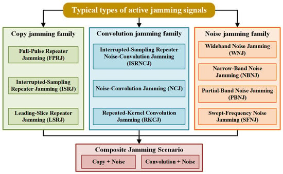
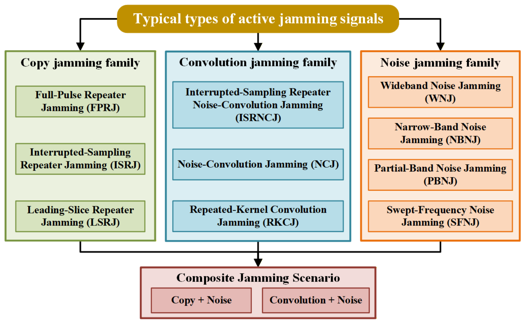
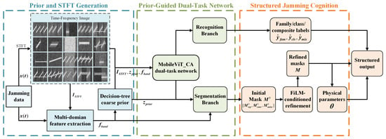
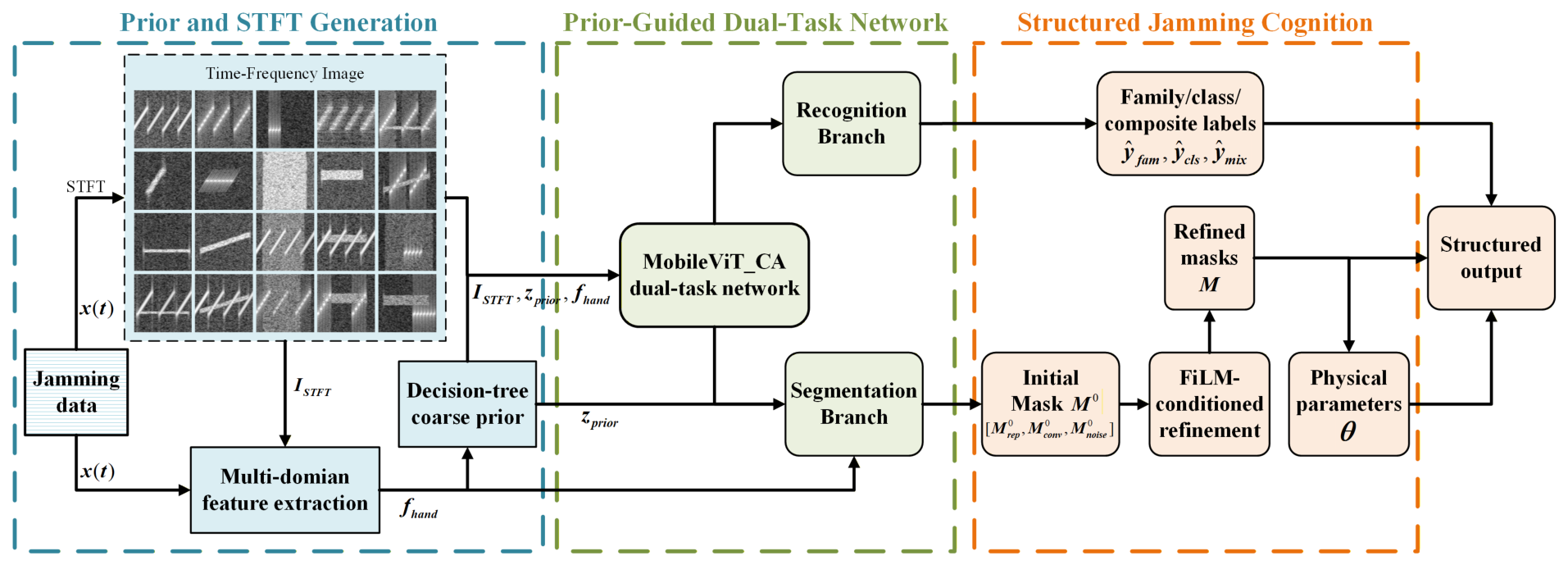
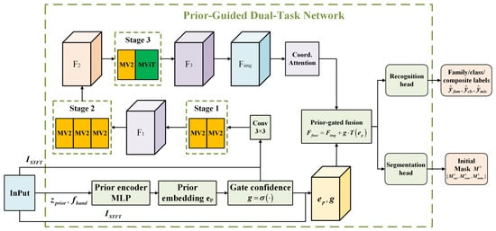
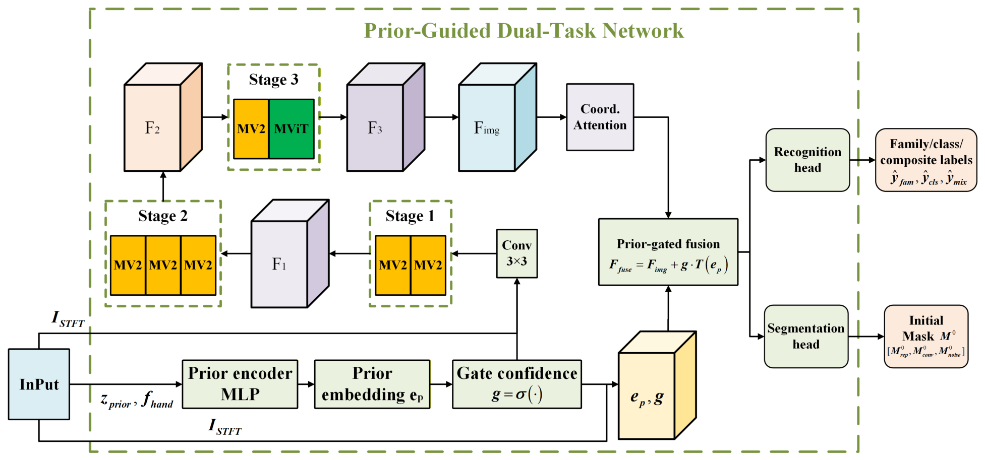
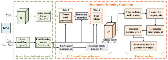
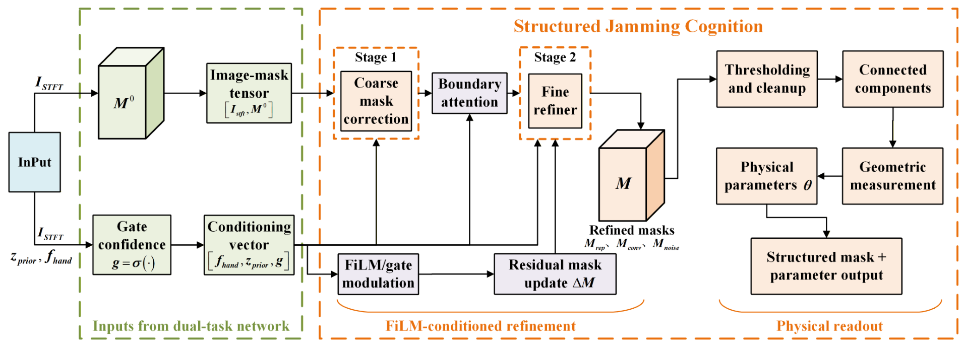
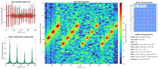
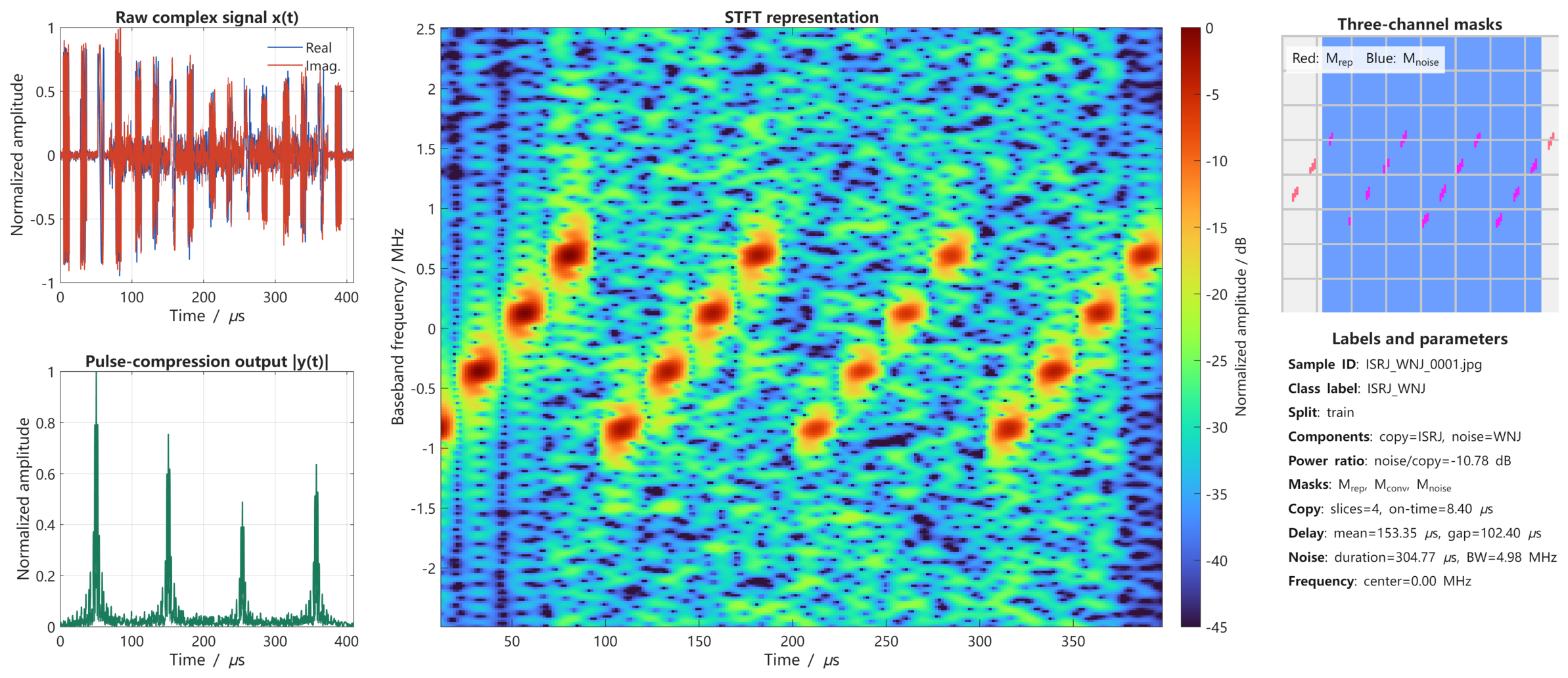
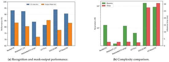
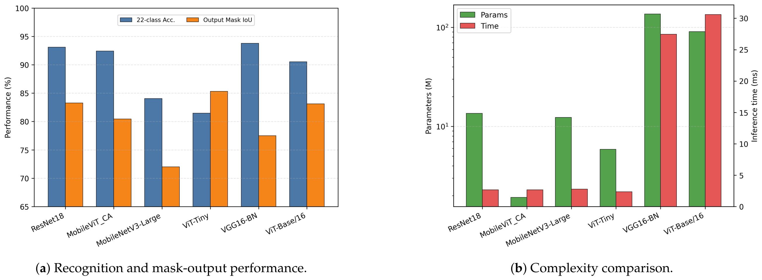
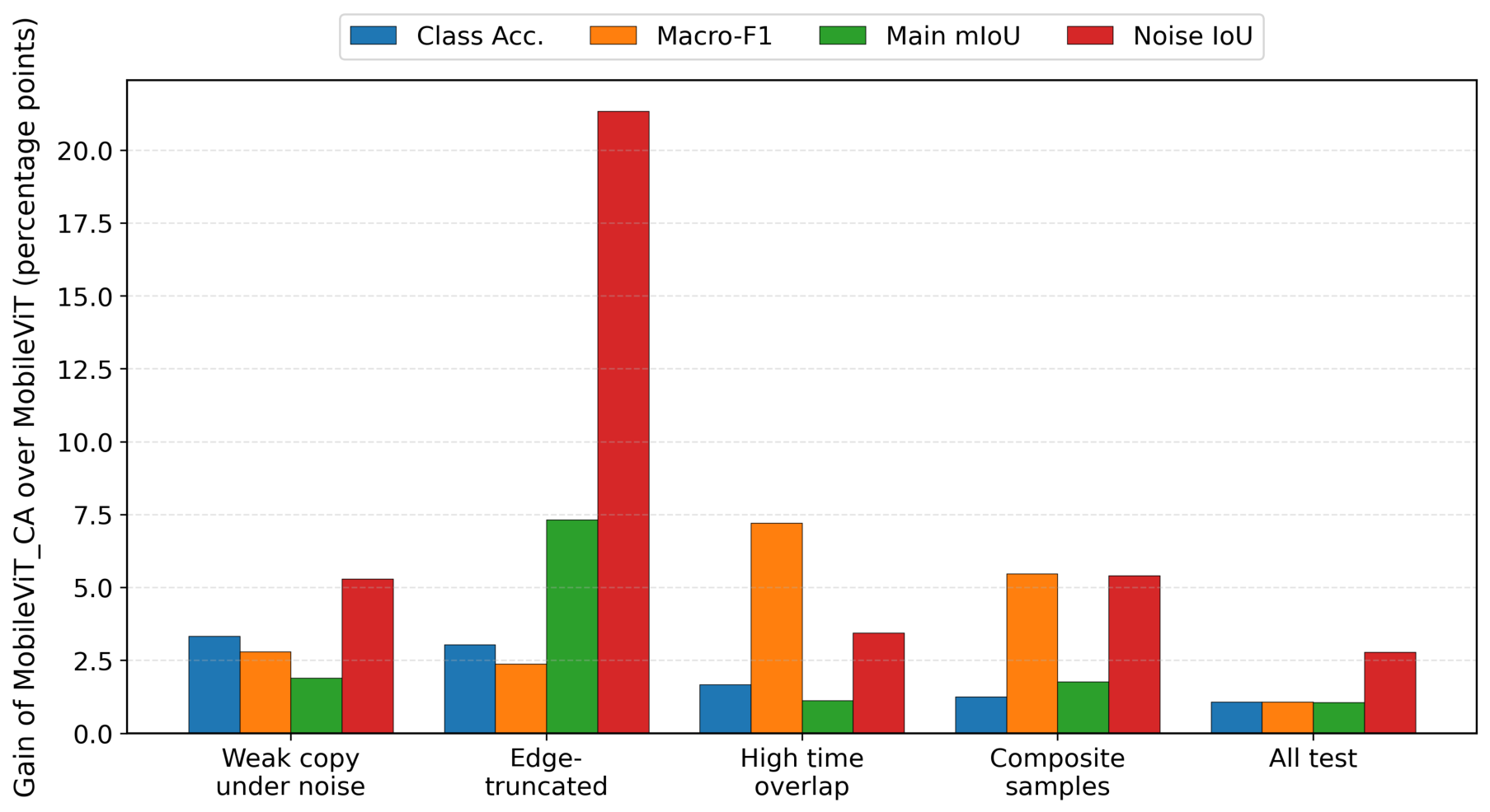
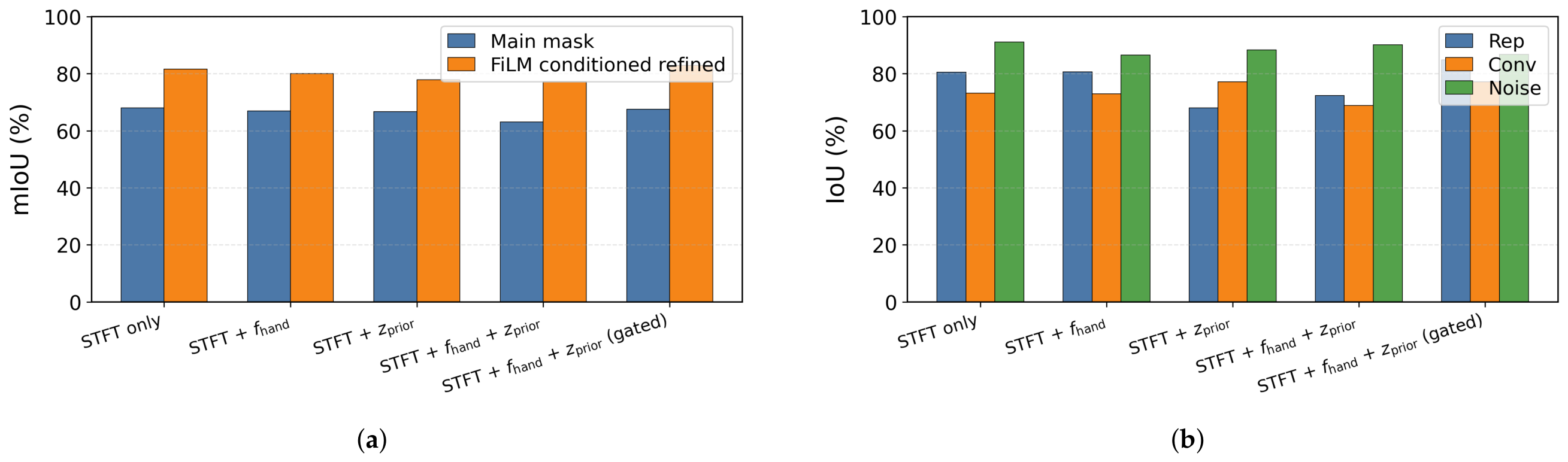
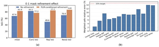
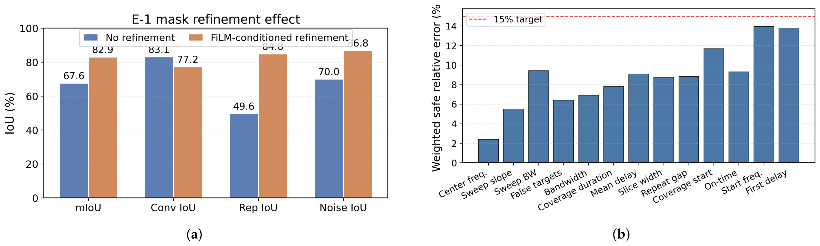
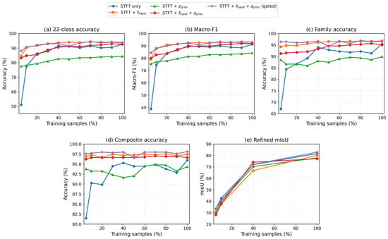
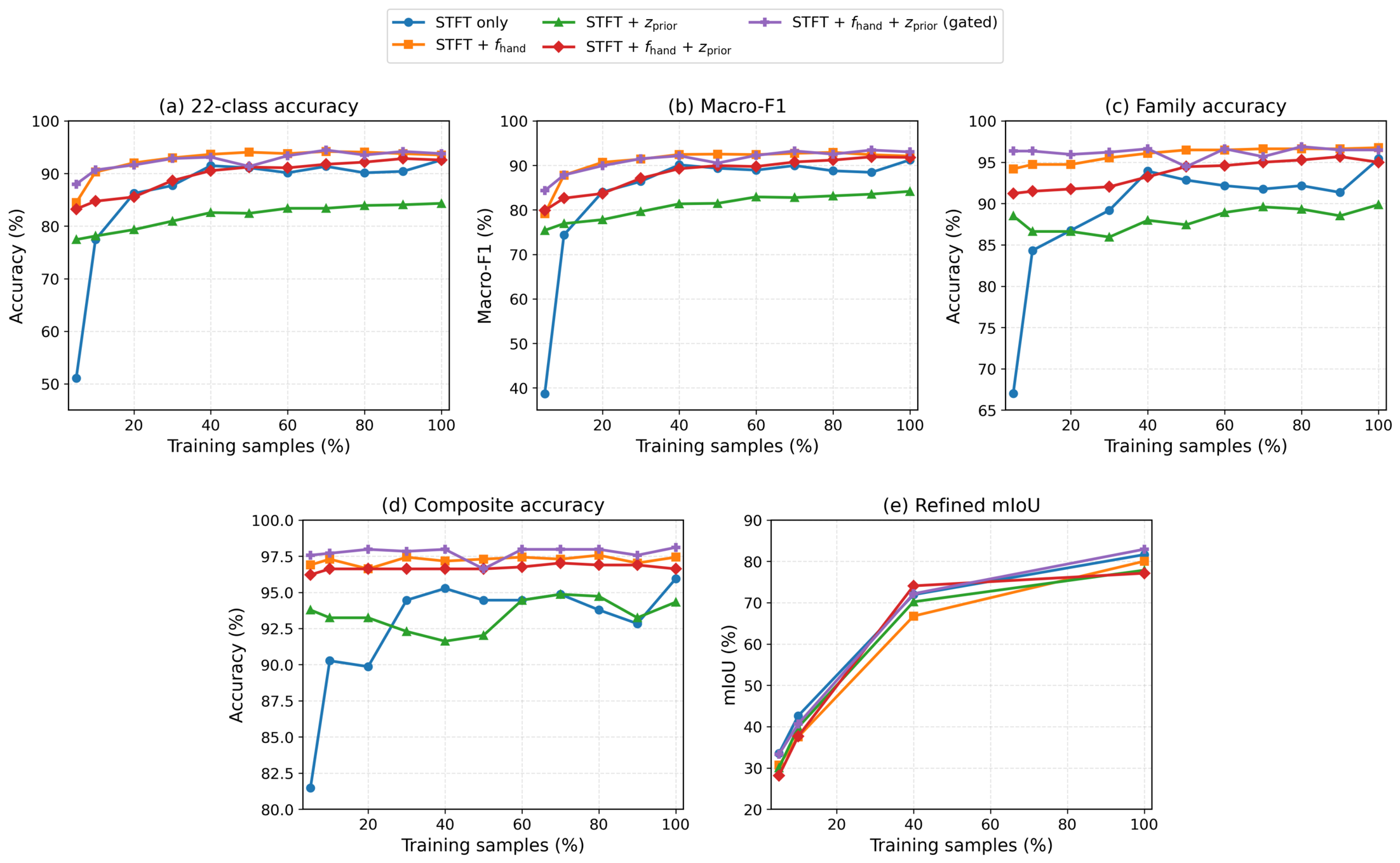
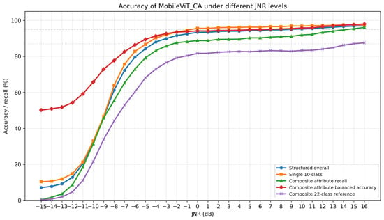
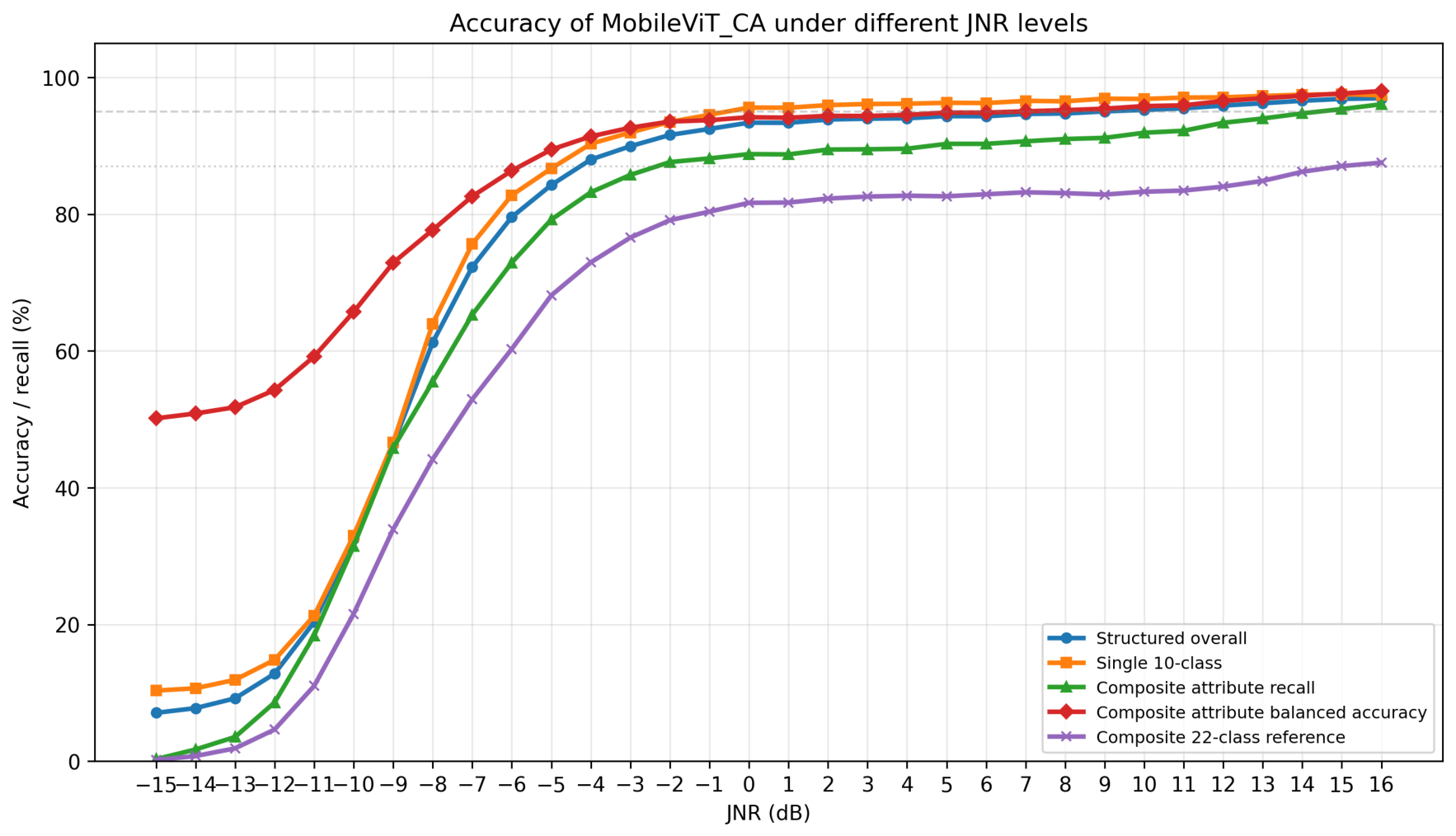
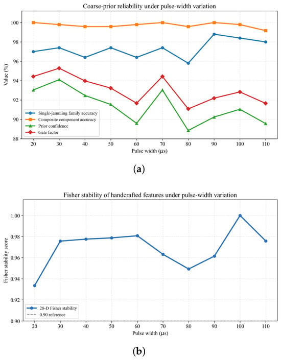
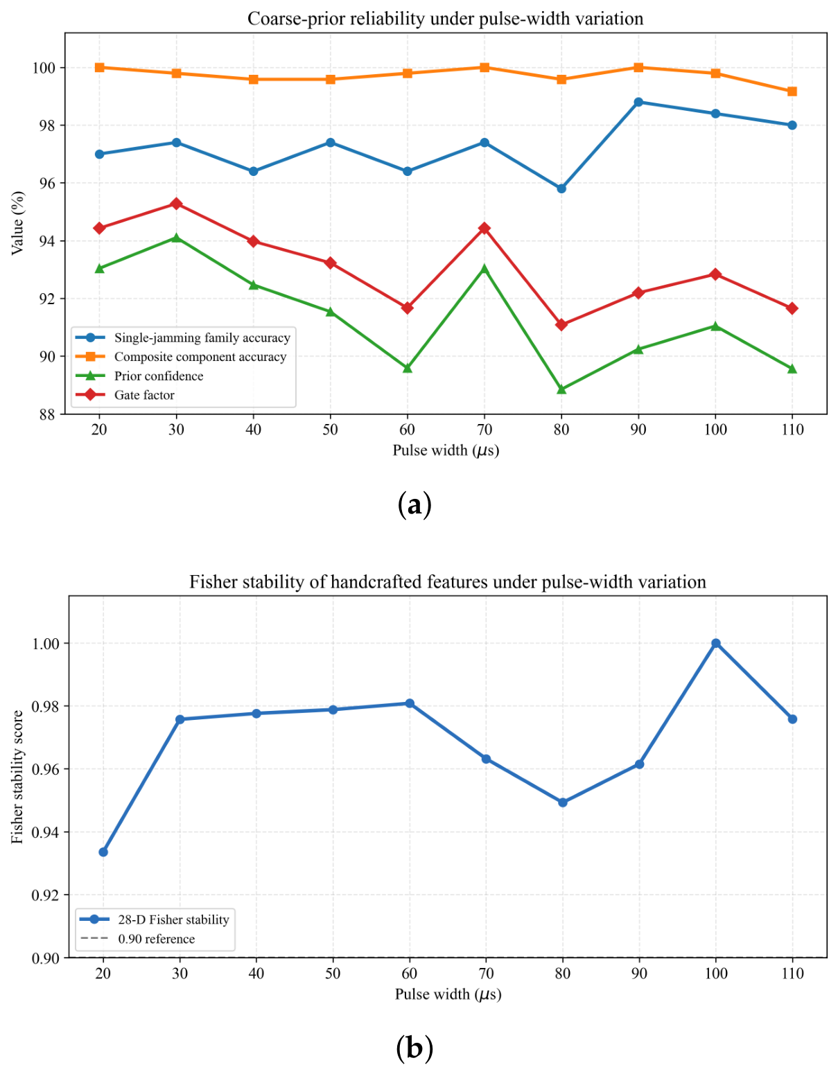
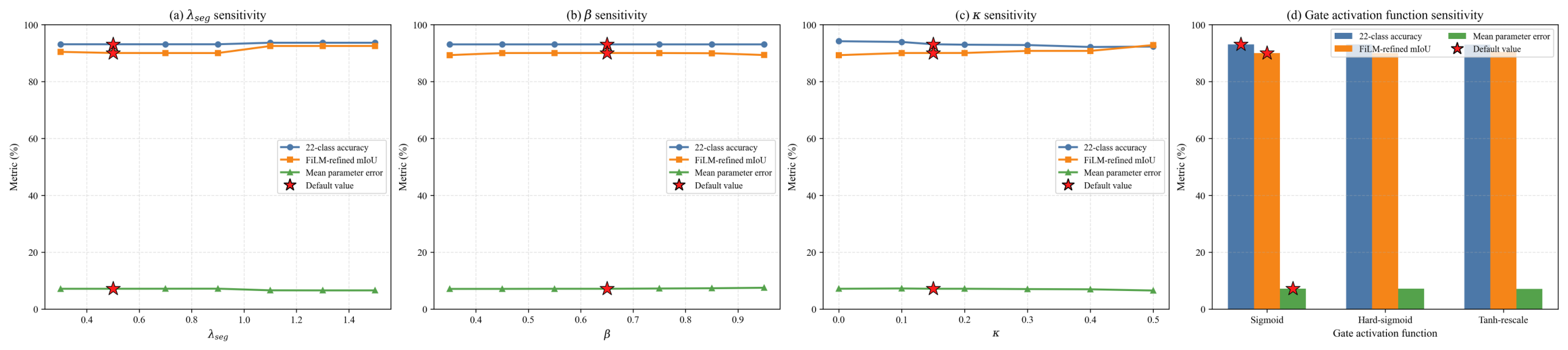

Disclaimer/Publisher’s Note: The statements, opinions and data contained in all publications are solely those of the individual author(s) and contributor(s) and not of MDPI and/or the editor(s). MDPI and/or the editor(s) disclaim responsibility for any injury to people or property resulting from any ideas, methods, instructions or products referred to in the content. |
© 2026 by the authors. Licensee MDPI, Basel, Switzerland. This article is an open access article distributed under the terms and conditions of the Creative Commons Attribution (CC BY) license.