Mitigating Class Imbalance and False-Negative Supervision in Remote Sensing Semantic Segmentation Using Object-Centric Patch Sampling

Highlights

What are the main findings?

• Object-centric patch sampling anchors each training patch to the geometric centroid of an annotated object, ensuring that every anchored patch contains at least one target instance. This keeps sampling concentrated around verified annotations and reduces the risk of false-negative supervision from incompletely labeled regions.
• The method was tested on satellite, aerial, and UAV imagery using both U-Net and DeepLabV3+. It consistently achieved higher IoU and F1-scores than sliding-window and random sampling across all configurations, with IoU improvements of up to 19.6 percentage points.

What are the implications of the main findings?

• The results show that how training patches are selected can be as important as, or even more important than, the number of patches used. Patch sampling should therefore be considered an important part of the segmentation methodology rather than simply a preprocessing step.
• The method does not require changes to the network architecture, loss function, or training procedure. Because it only changes how the training data are sampled, it can be incorporated into existing segmentation workflows with little to no additional computational cost.

Abstract

In Deep Learning Remote Sensing, data quantity is rarely the limiting factor. A single high-resolution satellite image can yield thousands of training patches. What determines model performance, yet remains largely overlooked, is the quality of those patches. To date, the choice of sampling method has rarely been treated as a methodological decision. Conventional approaches, namely sliding-window and random sampling, introduce two compounding data-quality problems: severe class imbalance caused by the overproduction of background-only patches and negative learning arising from incomplete annotations, where unlabeled objects are implicitly treated as negative examples during training. To address these limitations at the data construction stage, we propose object-centric patch sampling, a model-independent strategy that anchors each training patch to the geometric centroid of an annotated object. This design ensures that every object-anchored patch contains at least one target instance and substantially reduces exposure to unlabeled regions that generate false-negative supervision signals; only a small, deliberately controlled proportion of background-only patches is retained to preserve contextual variety without reinstating background dominance. The method is evaluated on three heterogeneous remote sensing datasets spanning satellite (Sentinel-2, 10 m), aerial (NAIP, 1 m), and UAV (0.25 m) imagery, covering cotton field segmentation, rural building extraction, and water body delineation, respectively. Using a U-Net architecture under identical training conditions, the proposed approach achieves IoU scores of 0.929, 0.896, and 0.912 on the three datasets, respectively, outperforming sliding-window sampling by up to 19.6 percentage points in IoU and consistently delivering higher F1-scores across all experimental configurations. Evaluation under DeepLabV3+ gives a mean IoU of 0.9504 and a mean F1-score of 0.9772 in a multi-class segmentation task, indicating that the gains are not specific to a single architecture. Unlike model-level solutions such as focal loss or class reweighting, the proposed method improves training data quality at its source and integrates seamlessly into any deep learning pipeline without architectural modifications.

1. Introduction

High-resolution remote sensing imagery has become one of the most powerful technologies for Earth observation, supporting applications in urban planning and mapping, crop monitoring in agriculture, hydrological analysis, and disaster risk assessment [1,2,3] and related applications. These capabilities have been further accelerated by recent advances in deep learning [4], which allow automated feature extraction from large and complex geospatial datasets [4,5]. Such deep learning methods have been widely applied to water-related remote sensing tasks, including flood inundation mapping and water body extraction [6,7]. Due to the high spatial resolution of remote sensing images and limited memory resources, most existing deep learning pipelines adopt a patch-based training strategy [8], where tiling, that is, the partitioning of large images into smaller patches that fit in memory [9], is performed before model ingestion.

Despite its widespread adoption, patch-based learning introduces a critical yet underexplored challenge: the strategy used to sample training patches fundamentally determines the quality, balance, and reliability of the training data. In most existing studies, patch extraction is treated as a preprocessing detail rather than a methodological component, with sliding-window [10] or random sampling [11] employed by default. The sliding-window approach prioritizes spatial coverage but often generates a large proportion of background-only samples, particularly in sparse-object scenarios [12,13] such as rural settlements or isolated water bodies. Similarly, random sampling frequently fails to capture true-positive regions [11].

The consequences of such sampling strategies are threefold. First, the dominance of background patches leads to severe class imbalance, biasing the learning process and slowing convergence [14]. Second, exhaustive patch generation significantly increases computational cost, inflating storage requirements, input/output overhead, and training time [4,15]. Third, and most critically, conventional sampling implicitly assumes complete and accurate annotations. In practice, however, remote sensing labels are frequently incomplete due to manual digitization errors, temporal inconsistencies, or budgetary constraints [16,17,18]. Under sliding-window or random sampling, unlabeled objects embedded within patches are incorrectly treated as negative examples, resulting in negative learning that degrades model generalization [19,20]. Several studies have attempted to mitigate class imbalance using loss reweighting [12], focal loss [21], oversampling strategies [22], or complex pseudo-label correction frameworks [23]. While effective to some extent, these methods operate at the model optimization level and do not address noise introduced at the data construction stage.

To address these limitations fundamentally at the source, we propose a principled, efficient, and comprehensive approach to image patch generation for semantic segmentation of remote sensing imagery. The proposed method constructs patches based on the geometric centroid of annotated objects. For every labeled polygon, the geometric centroid is computed, and a fixed-size image patch is extracted with this centroid at its center.

This sampling mechanism ensures that every extracted patch contains at least one target object. As a result, the generated dataset becomes object-centric rather than background-focused. Furthermore, because sampling is restricted to the neighborhood of annotated objects, the probability of including an unlabeled object within a background region is substantially reduced, which minimizes false-negative supervision during training. Rather than modifying the model architecture or rebalancing class weights [12], the proposed method improves the quality of the training data at its source. To address the creation of excessive foreground dominance and reduce the risk of model overfitting, approximately 20% additional background-only patches were deliberately introduced during training. This controlled inclusion of background samples preserves a more balanced representation of foreground and background classes while retaining the object-centric character of the dataset. The proposed strategy is evaluated across three representative remote sensing tasks: cotton field delineation in an agricultural landscape of Australia, building extraction in rural areas of the United States, and water body extraction in flood-prone regions of Nepal, using satellite imagery, aerial photographs, and UAV imagery, respectively.

The evaluation is extended to a second architecture and to a multi-class task in order to examine how object-centric patch sampling behaves across different spatial scales, class complexities, and network types. Specifically, we benchmark lightweight encoder–decoder models (U-Net) [9] alongside dilated multi-scale feature extractors (DeepLabV3+ [24] equipped with an ImageNet-pretrained ResNet-50 backbone and Atrous Spatial Pyramid Pooling). We also extend the framework to a multi-class setting ($K\in \left\{\mathrm{Cotton},\mathrm{Water}\right\}$, together with background) by anchoring patch extraction to each target category in turn. This scheme maintains proportional representation across the target categories and allows the effect of object-centric sampling to be examined when several classes occur within the same scene.

1.1. Related Works

1.1.1. Patch-Based Training in Remote Sensing

Patch-based training has become standard practice in remote sensing deep learning due to the high spatial resolution of satellite and aerial imagery and the memory constraints of modern GPUs [8]. Sliding-window sampling was popularized by early object detection pipelines [25] and remains the default preprocessing step in many segmentation frameworks [9,10]. Zhang et al. [8] demonstrated that patch size and stride significantly influence segmentation accuracy in urban land use classification. Ji et al. [5] showed that multi-source aerial datasets require careful patch overlap strategies to avoid boundary artifacts. Despite the prevalence of patch-based pipelines, the choice of sampling strategy itself has received little systematic attention compared to architectural design.

1.1.2. Class Imbalance in Remote Sensing Segmentation

Class imbalance is a well-documented challenge in remote sensing segmentation, where foreground objects (buildings, crops, and water bodies) often constitute a small fraction of the total image area [14]. Buda et al. [12] conducted a systematic study of class imbalance in convolutional neural networks and found that both oversampling and loss reweighting consistently improve performance. Lin et al. [21] proposed Focal Loss, which down-weights easy background examples and focuses training on hard foreground cases, achieving state-of-the-art results in dense object detection. He and Garcia [22] provided a comprehensive survey of imbalanced learning strategies. Zhou et al. [14] proposed a dynamic class-balanced loss specifically for remote sensing segmentation. However, all of these solutions operate at the model optimization level and do not prevent the underlying data imbalance from being constructed in the first place.

1.1.3. Label Noise and Negative Learning

Label noise in training data is a fundamental challenge for deep learning models [17]. Rolnick et al. [17] demonstrated that deep networks are surprisingly robust to random label noise but are highly sensitive to systematic biases, such as consistent misclassification of a particular class. Northcutt et al. [18] introduced confident learning as a principled framework for estimating and correcting label errors. Kim et al. [19] studied negative learning, defined as the phenomenon in which incorrect complementary labels actively degrade model performance, and showed that even a small proportion of systematically mislabeled samples can cause significant generalization loss. In remote sensing, Zhu et al. [16] identified incomplete annotation as a primary source of label noise, arising from the practical difficulty of exhaustively labeling all objects across large-area imagery. The present work addresses this problem not through label correction but through a sampling strategy: by avoiding patches where unlabeled objects are present.

1.1.4. Data-Centric Learning

Recent years have seen growing interest in data-centric AI, which emphasizes improving training data quality rather than model architecture [26]. Curriculum learning [27] proposes ordering training samples by difficulty to improve convergence. Active learning [28] selects the most informative samples for annotation to reduce labeling cost. In general computer vision, foreground-focused data preparation is well-established; object detection pipelines routinely crop around labeled bounding boxes for instance augmentation, and frameworks such as MM Segmentation [29] offer ROI-based sampling transforms. However, these techniques typically isolate tight, variable-sized target boundaries rather than generating the fixed-extent, context-preserving patches required by deep semantic segmentation backbones.

In remote sensing, data-centric methodologies remain vastly underexplored relative to model-centric innovations. Large-format georeferenced rasters paired with sparse GIS vector annotations cause conventional sliding-window grids to suffer from severe class imbalance and false-negative supervision from unannotated background areas [30]. The proposed object-centric sampling framework contributes to data-centric remote sensing research through an automated vector-raster centroid coupling pipeline. By dynamically anchoring uniform patches to topological centroids, the workflow automatically suppresses uninformative background expanse, eliminates edge-padding feature distortion near tile boundaries via inward centroid displacement, and formally demonstrates that an annotation-driven sampling decision can yield substantial accuracy gains without any modification to the model architecture, loss function, or training procedure.

1.1.5. Distinction from Existing Foreground-Aware Sampling

Foreground-aware sampling strategies in computer vision and remote sensing typically address class imbalance through downstream model or algorithmic adjustments [11,15]. These methods rely on modified network architectures (such as feature-masking modules or auxiliary foreground attention heads), loss-level reweighting, or dynamic batch sampling during network training. While effective at directing network focus, these approaches have two limitations: (1) they require full raster scenes or background-dominated tiles to pass through data-loading and feature-extraction pipelines before foreground filtering occurs, incurring high computational memory overhead, and (2) they alter network architecture or loss function design, limiting model modularity. In contrast, the proposed object-centric patch sampling operates upstream, at the data ingestion stage. Rather than modifying network architectures or computing online foreground attention masks during training, our method uses target vector centroids (xk, yk) as spatial anchors to extract fixed-extent patches prior to dataset creation. By filtering background at its source, this approach ensures that every patch contains at least one target and reduces false-negative supervision while remaining architecture-agnostic so that standard segmentation models can be used without custom loss functions or modified training routines.

2. Methodology

In this section, we first formalize the problem setting and then describe conventional sampling strategies used for comparison. We then introduce the proposed object-centric sampling method, describe its implementation, and analyze its computational properties.

2.1. Problem Formulation

Let the remote sensing image be denoted $I\in R^{H\times W\times C}$, where H, W, and C denote the image height, width, and number of spectral bands, respectively, and R indicates that each pixel takes a real value. In constructing the training samples, the objects of interest, such as buildings, agricultural fields, or water bodies, are first annotated. Let the set of annotated polygons be denoted $L={\left\{P_k\right\}}_{k=1}^N$, where N is the total number of annotated polygons.

A deep learning model is trained on a large number of patches of size s × s with batch size k. So, we must construct a training dataset $\mathcal{D}=\{\left(X_i,Y_i\right){\}}_{i=1}^M$ where $X_i\in R^{S\times S\times C}$ is an image patch of fixed spatial size s × s, and $Y_i\in \{\mathrm{0,1}{\}}^{s\times s}$ is the corresponding label mask.

The objective of patch sampling is to generate a dataset $\mathcal{D}$ that maximizes learning efficiency and generalization performance [31]. In practice, however, conventional sampling strategies implicitly assume that every object in an image is labeled, and the background regions are equally informative as foreground regions. In practice, these assumptions give rise to class imbalance, inflated dataset size, and negative learning in real-world remote sensing datasets. The proposed object-centric patch sampling technique addresses these issues by constructing each patch around the centroid of a labeled polygon.

2.2. Conventional Patch Sampling Strategies

For comparative evaluation, we consider two widely used patch sampling strategies: sliding-window sampling and random sampling.

2.2.1. Sliding-Window Sampling

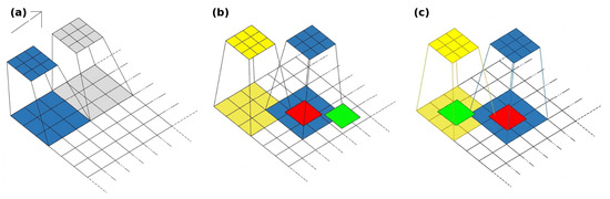
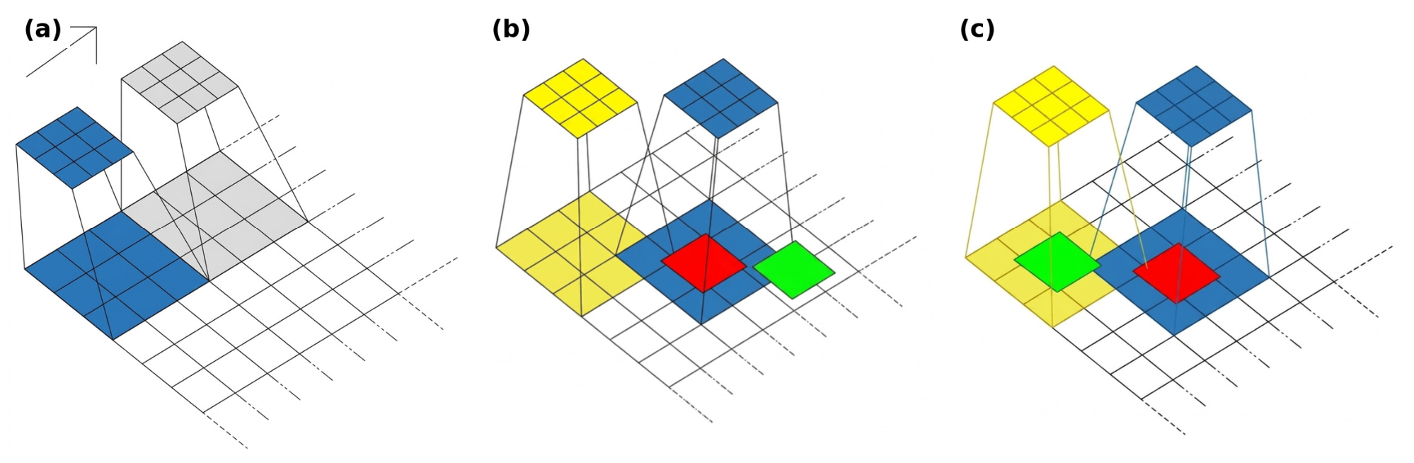
As illustrated in Figure 1a, sliding-window sampling extracts patches by raster-scanning the image with a fixed stride t, such that overlapping patches are generated to ensure full spatial coverage [25]. Formally, patch centers are placed at locations $\left(x_i,y_j\right)=\left(i\cdot t,j\cdot t\right),\hspace{1em}i,j\in Z^{+}$. While this approach guarantees complete coverage, it typically produces a large number of background-only patches in sparse-object scenarios. Moreover, patches overlapping unlabeled objects are implicitly treated as negative samples, introducing systematic label noise during training.

2.2.2. Random Patch Sampling

As shown in Figure 1b, random sampling selects patch centers uniformly from the image domain until a predefined number of patches is reached. This strategy reduces redundancy and dataset size relative to sliding-window extraction. However, it provides no guarantee that all labeled objects are adequately represented, and the result remains sensitive to the random seed [27]. Like sliding-window sampling, random extraction does not prevent unlabeled objects from appearing within negative samples.

2.3. Object-Centric Patch Sampling

2.3.1. Conceptual Overview

As shown in Figure 1c, the object-centric patch sampling strategy constructs training patches by anchoring them to labeled object locations rather than to image coordinates. The key idea is to ensure that each extracted patch contains at least one target object, thereby maximizing informational content and eliminating background-only samples. Let $P_i$ be a targeted polygon defined by an ordered set of n discrete boundary vertices $V_i=\{\left(x_0,y_0\right),\left(x_1,y_1\right),\dots ,\left(x_{n-1},y_{n-1}\right)\}$, where $\left(x_n,y_n\right)=\left(x_0,y_0\right)$ close the boundary. The signed planar area $A_i$ of $P_i$ is calculated via the discrete Shoelace formula [32].

$$A_i={\displaystyle \frac{1}{2}}\sum _{k=0}^{n-1}\left(x_k{y}_{k+1}-x_{k+1}{y}_k\right)$$

The geometric centroid $C_i=\left(C_{x,i},C_{y,i}\right)$ of polygon $P_i$ is then computed directly from the corresponding first-order moments [33] as

$$C_{x,i}={\displaystyle \frac{1}{6A_i}}\sum _{k=0}^{n-1}\left(x_k+x_{k+1}\right)\left(x_k{y}_{k+1}-x_{k+1}{y}_k\right)$$

$$C_{y,i}={\displaystyle \frac{1}{6A_i}}\sum _{k=0}^{n-1}\left(y_k+y_{k+1}\right)\left(x_k{y}_{k+1}-x_{k+1}{y}_k\right)$$

For each centroid $C_i$, a patch $W_i$ of size s × s is extracted with $C_i$ as its center. The corresponding label mask $Y_k$ is generated by rasterizing the polygon $P_k$ within the patch extent [34].

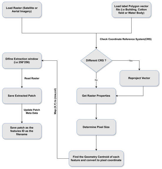
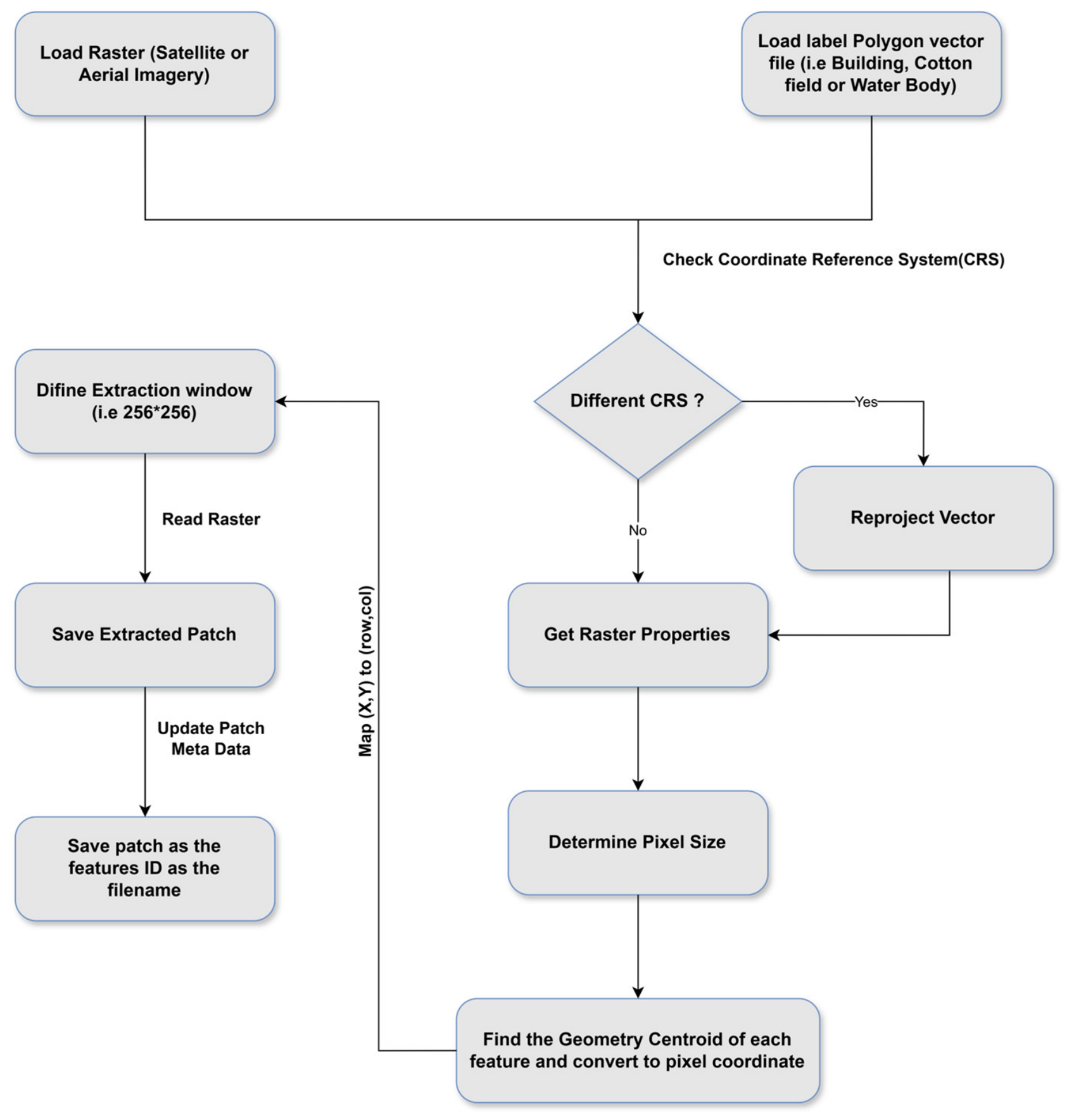
This design ensures that every training sample contains a positive instance, directly addressing class imbalance and eliminating false-negative supervision arising from unlabeled objects. The complete processing workflow is summarized in Figure 2.

2.3.2. Boundary and Edge Handling

In practice, object centroids may lie near image boundaries, causing partial patches to extend beyond the image domain. To address this issue, centroid coordinates are adjusted as follows:

$$x_k^{\prime }=min\left(max\left(x_k,s/2\right),w-s/2\right),$$

(1)

$$y_k^{\prime }=min\left(max\left(y_k,s/2\right),H-s/2\right)$$

(2)

This inward shift preserves patch completeness while maintaining proximity to the target object. Unlike padding-based solutions, centroid correction avoids introducing artificial pixel values at patch boundaries.

2.3.3. Handling Dense or Overlapping Objects

In scenes containing dense object clusters (e.g., adjacent building footprints), multiple target centroids often lie in close proximity, resulting in redundant, near-identical patch extractions. To eliminate this redundancy, any pair of centroids separated by a spatial distance below $d_{min}=32$ pixels is merged into a single cluster center $C_{\mathrm{merged}}$. For a standard patch size of $s=256$ pixels, $d_{min}=32$ pixels represent 12.5% of the patch dimension; unmerged patches separated by less than this threshold overlap by more than 87.5% in area without adding distinct contextual information.

A bounded random offset of $\left({\delta }_x,{\delta }_y\right)\sim U\left(-\mathrm{16,16}\right)$ pixels is applied to $C_{\mathrm{merged}}$. Given the 128-pixel half-width of a $256\times 256$ patch, a maximum displacement of 16 pixels leaves a margin of at least 112 pixels (128 − 16) between the object center and the nearest patch boundary. Target objects that fall within this radius therefore remain fully enclosed in the patch, while the offset introduces some variation in the surrounding context.

2.3.4. Mitigation of Negative Learning from Incomplete Labels

A critical advantage of object-centric sampling is its robustness to incomplete annotations. Consider an image containing N true objects, of which only $N_a<N$ are annotated. Under sliding-window or random sampling, patches containing unlabeled objects are frequently labeled as background, generating false-negative signals during training.

By restricting sampling to patches centered on annotated objects, the proposed method avoids sampling ambiguous background regions where unlabeled objects may exist. Consequently, the probability of negative learning due to annotation omission is substantially reduced.

2.3.5. Controlled Background Integration

A controlled allocation of 20% pure background patches is included in the training dataset to prevent foreground overfitting and to reduce false positives on spectrally ambiguous non-target terrain. Candidate background regions are selected using a strict spatial buffer criterion ($d_{\min }>\sqrt{2}\cdot {\displaystyle \frac{S}{2}}$ from any target boundary), so that no target pixels fall within the patch. Rather than sampling featureless terrain, background patches are mined across contextually diverse land-cover categories (e.g., bitumen roads, bare soil, and water bodies) identified via spectral variance filtering. In an ablation over background ratios, 20% gave the best trade-off, reducing false positives on hard background while maintaining recall and precision.

2.4. Experimental Setup

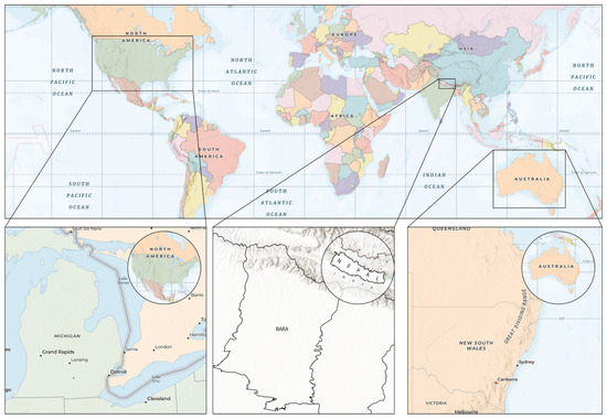
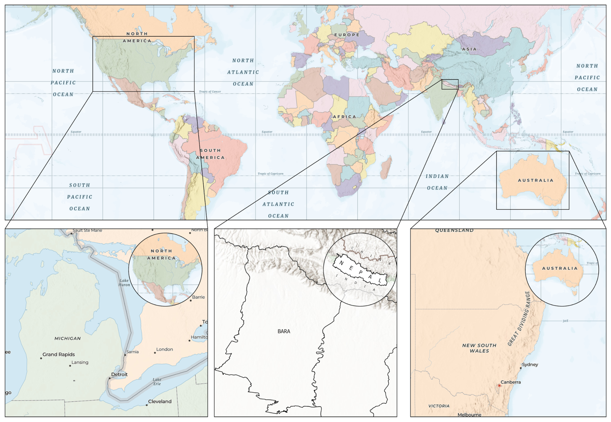
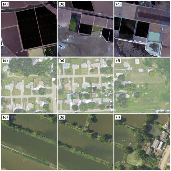
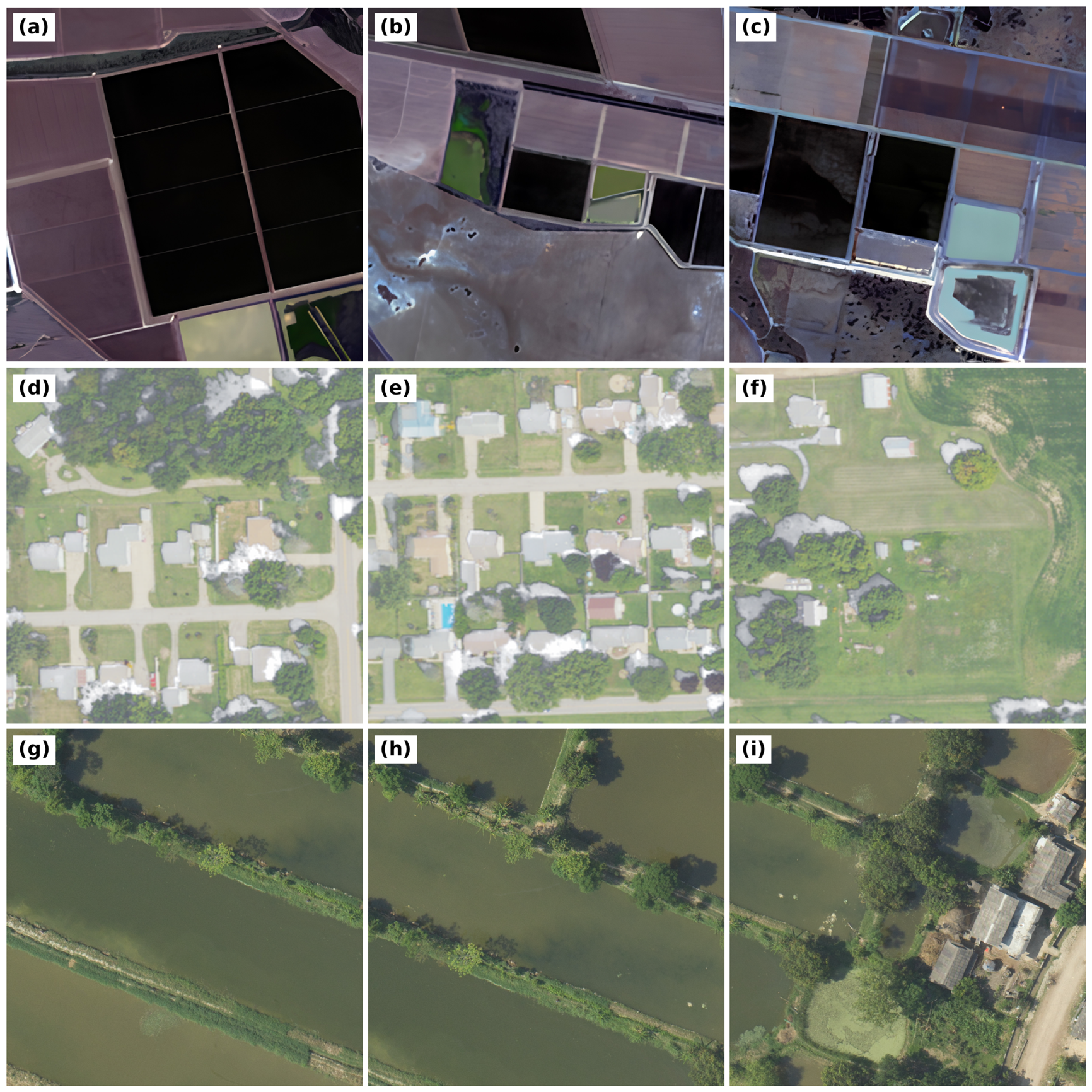
Controlled experiments were conducted on three heterogeneous remote sensing datasets: Sentinel-2 imagery [35] of Queensland, Australia, for cotton field segmentation; NAIP aerial imagery [36] of the USA for building segmentation; and UAV orthophoto imagery of the Terai region of Nepal for water body segmentation. The locations of the three study sites are shown in Figure 3, and representative samples of each dataset are presented in Figure 4. The datasets span a wide range of spatial resolutions (10 m, 1 m, and 0.25 m, respectively) and distinct object characteristics, including large homogeneous parcels (cotton fields), sparse and compact structures (buildings), and irregular, elongated features (water bodies).

Our evaluation framework is structured into two complementary experimental suites across three patch sampling strategies (sliding-window sampling, random sampling, and the proposed object-centric sampling):

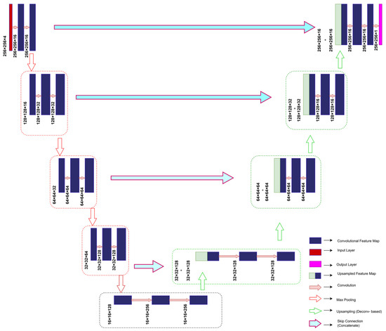
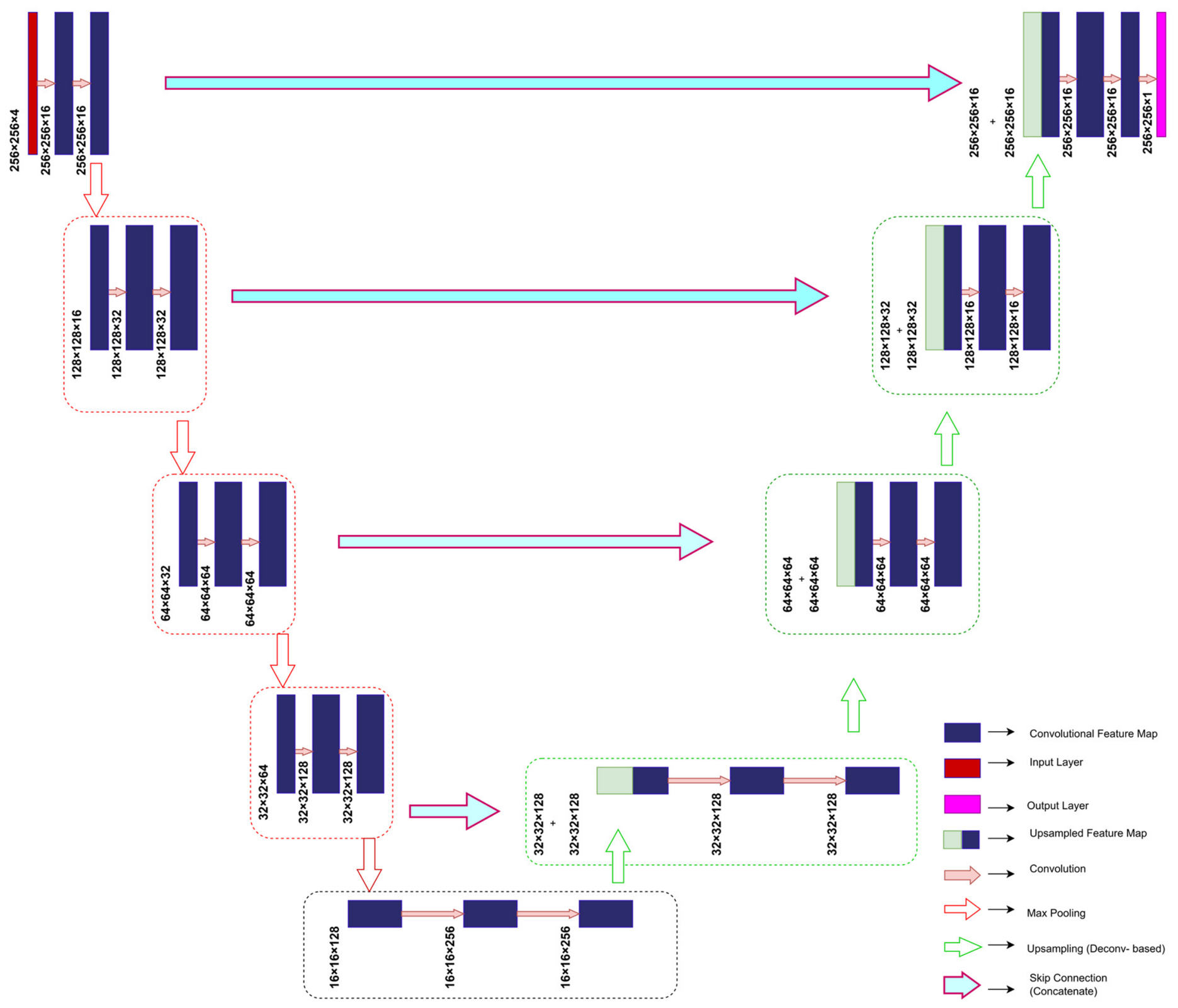
• Primary experiments (U-Net): Benchmark performance across the three individual target categories (cotton, buildings, and water) was established using a modified U-Net architecture (Figure 5) [9], adapted only in input/output dimensions, filter capacities, and pooling configurations.
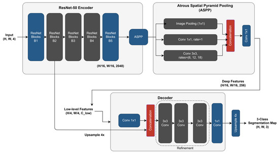
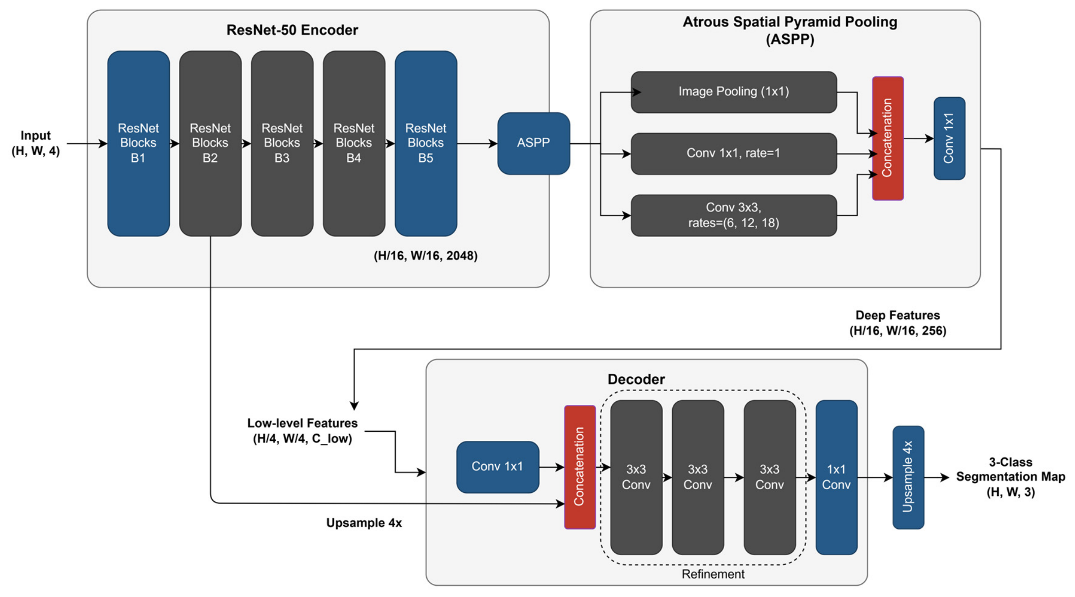
• Cross-architecture and multi-class experiments (DeepLabV3+): To test whether the sampling strategy remains effective under a different architecture and in a multi-class setting, further experiments were conducted using a DeepLabV3+ network equipped with an ImageNet-pretrained ResNet-50 backbone (Figure 6) [24]. This suite evaluated both single-class target detection (cotton) and a multi-class joint segmentation task where scene patches contained co-occurring cotton, water, and background classes.

The patch size was fixed at 256 × 256 pixels for the satellite and aerial imagery, and for the high-resolution drone orthophoto, we increased the patch size to 1024 × 1024 pixels to ensure that at least one complete object was contained within each patch. All experiments were conducted on a workstation equipped with an Intel Core i9-14900KF CPU and 64 GB of RAM, running Windows 10.

The U-Net model [9] was optimized using the Adam optimizer [37], a batch size of 32, and a maximum of 100 epochs. The learning rate was controlled by a scheduler with an initial value of 2 × 10⁻⁴, with a reduction factor of 0.2 and patience of 4 epochs, monitoring the validation loss. Early stopping [38] was applied to retain the best-performing model and to reduce training time. A hybrid loss combining the Dice coefficient and binary cross-entropy [39] was used as the optimization objective. To prevent spatial leakage, the datasets were partitioned at the scene level into 70% training, 20% validation, and 10% testing.

Segmentation performance was evaluated using pixel-level metrics, including Intersection over Union (IoU) [40], Dice coefficient, and F1-score. IoU was adopted as the primary metric due to its balanced sensitivity to false positives and false negatives. To isolate the effect of the sampling strategy from the loss function, all three sampling strategies were trained with the same mixed loss function (${\mathcal{L}}_{\mathrm{BCE}}+{\mathcal{L}}_{\mathrm{Dice}}$) under identical hyperparameters, optimizers, learning rates, and random seeds. In addition to predictive accuracy, computational efficiency was assessed by measuring total training time, convergence behavior, and peak memory usage. Partitioning was carried out at the scene level before any patch extraction, so that adjacent patches from the same image cannot appear in both the training and test sets, and no test patch shares geographic coverage with a training tile.

3. Results

For each dataset, the training and validation learning curves and the segmentation metrics obtained on the held-out set are compared across the three sampling strategies. Both learning dynamics and quantitative performance metrics are examined to determine how sampling strategy influences segmentation accuracy, convergence behavior, and overall model performance.

3.1. Sentinel-2 Cotton Field Segmentation

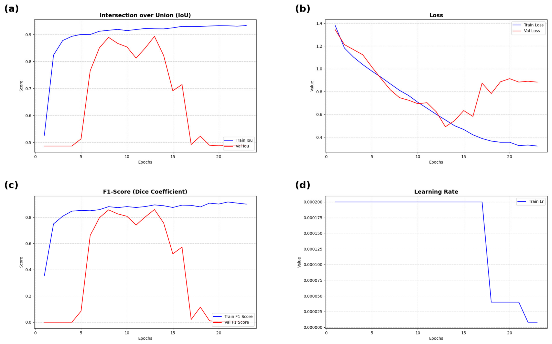
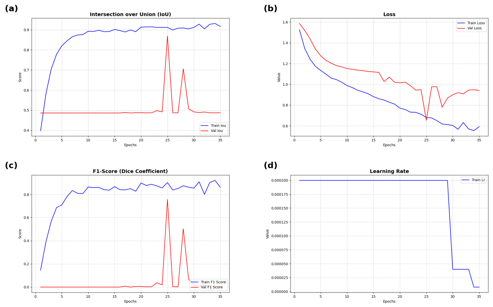
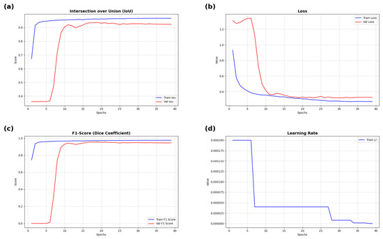
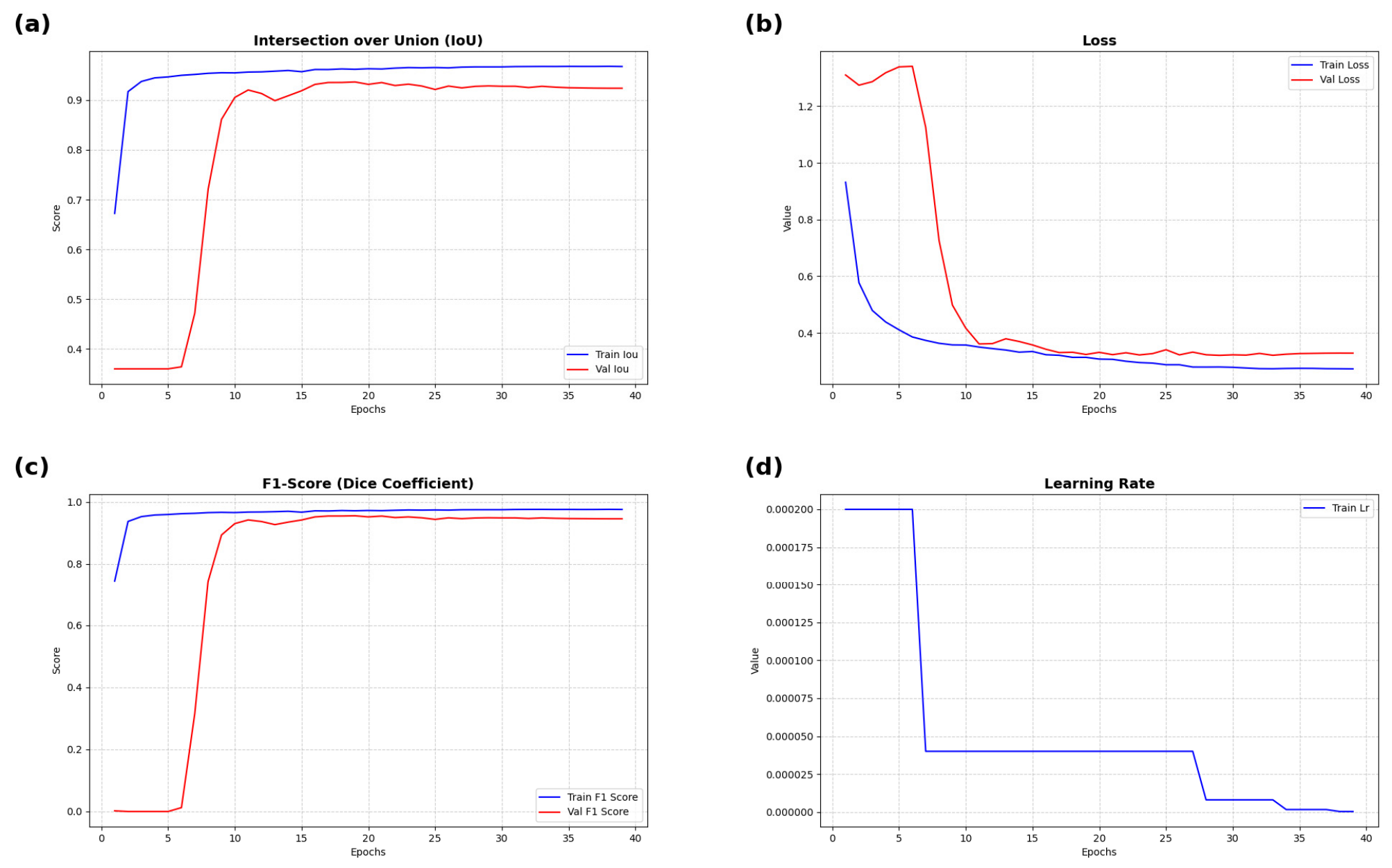
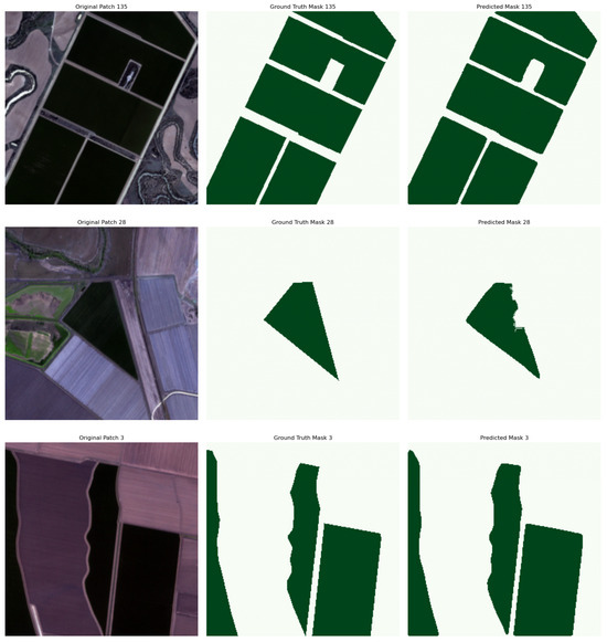
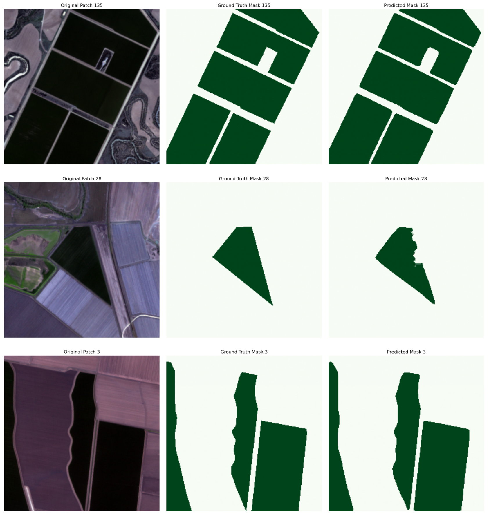
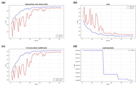
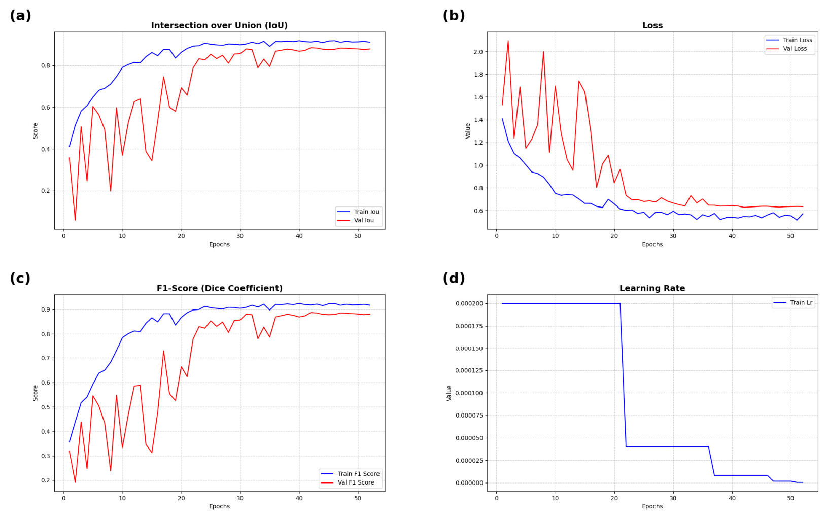
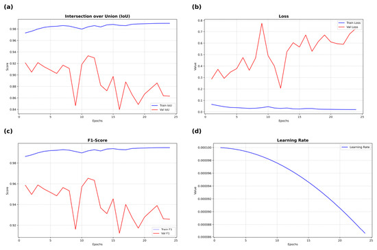
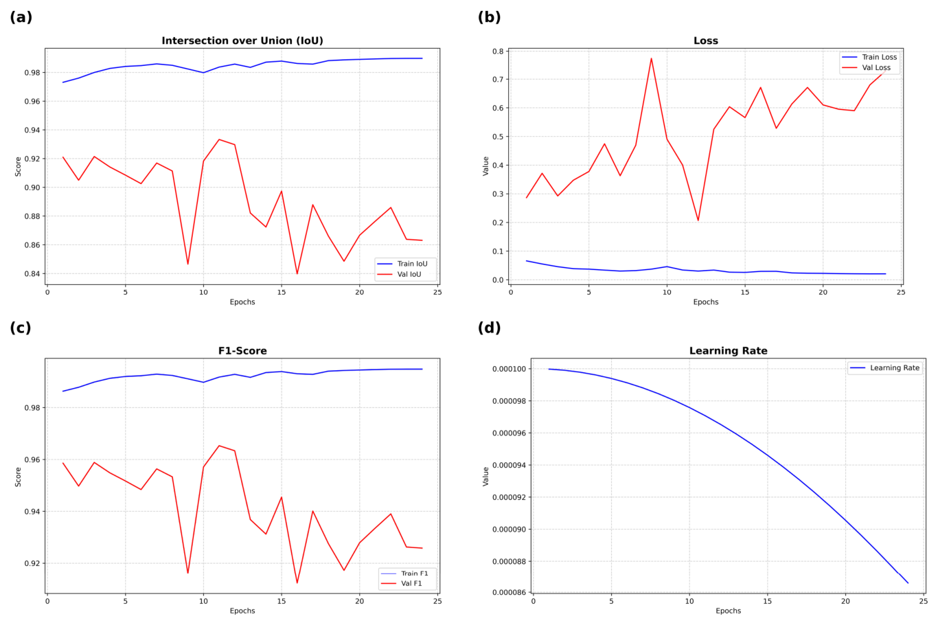
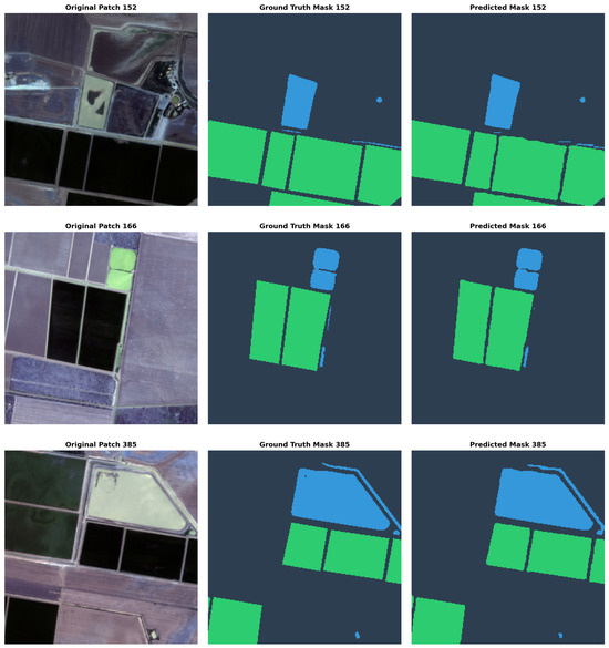
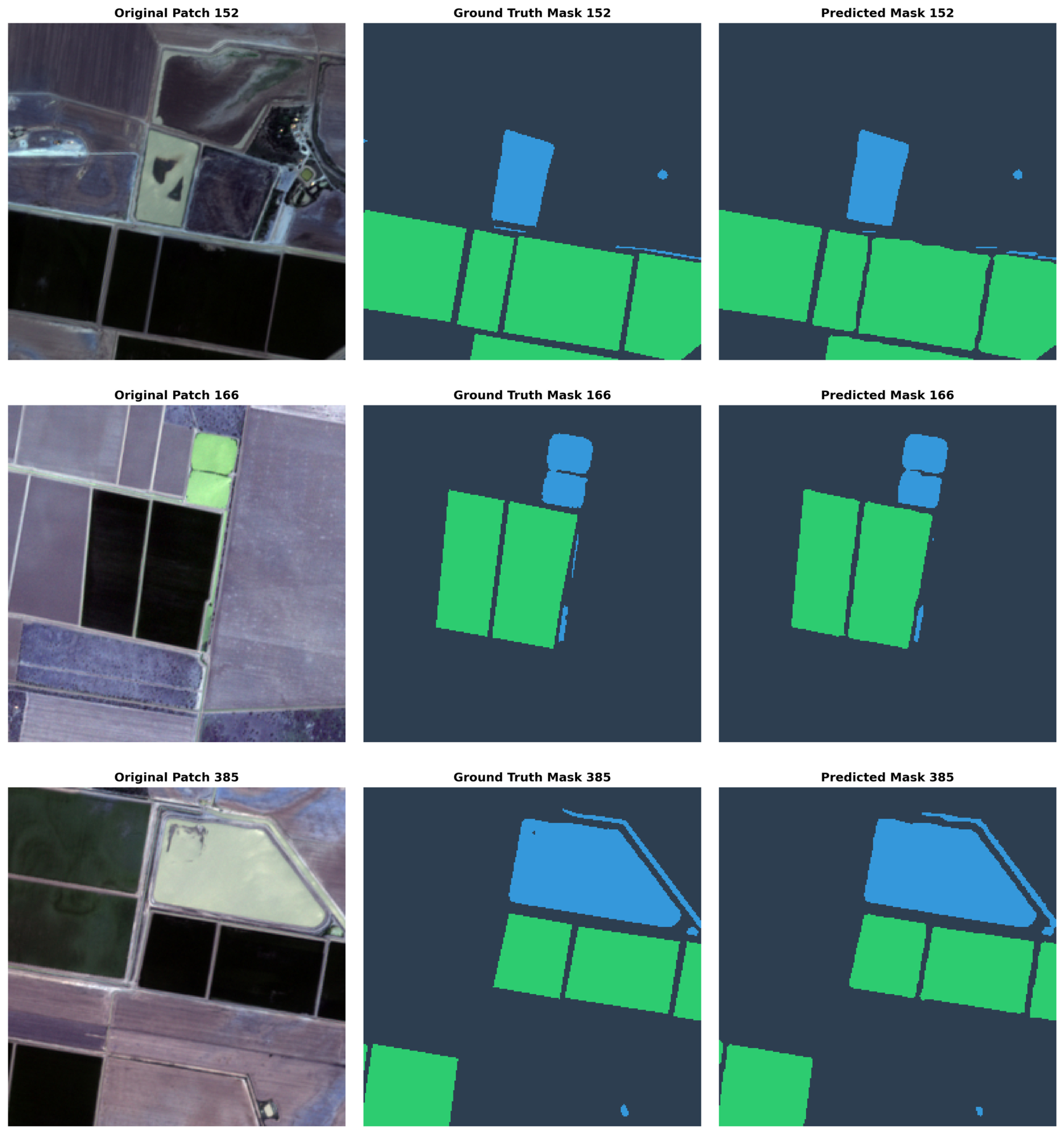
On the Sentinel-2 cotton field dataset, the three sampling strategies produced clearly different training dynamics (Figure 7, Figure 8 and Figure 9). With sliding-window sampling (Figure 7), the training metrics rose rapidly, but the validation IoU and F1-score oscillated and dropped in the later epochs, and the validation loss began to increase while the training loss continued to fall, indicating overfitting to the dominant background class. Random sampling (Figure 8) produced lower but more stable validation curves, whereas object-centric sampling (Figure 9) yielded smooth curves in which the validation and training metrics remained close throughout training. The corresponding metrics on the validation set are summarized in

Table 1. Segmentation performance on the Sentinel-2 validation dataset.

Sampling Strategy	IoU	Dice + BCE Loss	F1-Score	Epoch	Dataset Size	Training Time (min)
Sliding-window sampling	0.8930	0.4912	0.8595	23	5028	200.697
Random sampling	0.8687	0.6533	0.7565	35	1597	93.996
Object-centric sampling	0.9285	0.3207	0.9488	39	1597	108.271

. Object-centric sampling obtained the highest IoU (0.929) and F1-score (0.949), compared with 0.893 and 0.860 for sliding-window sampling and 0.869 and 0.757 for random sampling. It reached this accuracy from 1597 training patches, far fewer than the 5028 patches generated by sliding-window sampling, and with a shorter training time (108 min versus 201 min). A qualitative comparison is shown in Figure 10, where the predicted masks closely follow the reference field boundaries.

3.2. NAIP Building Segmentation

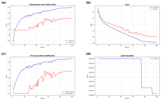
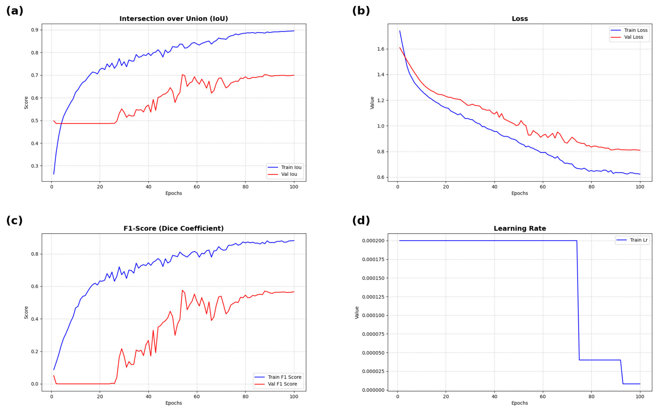
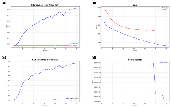
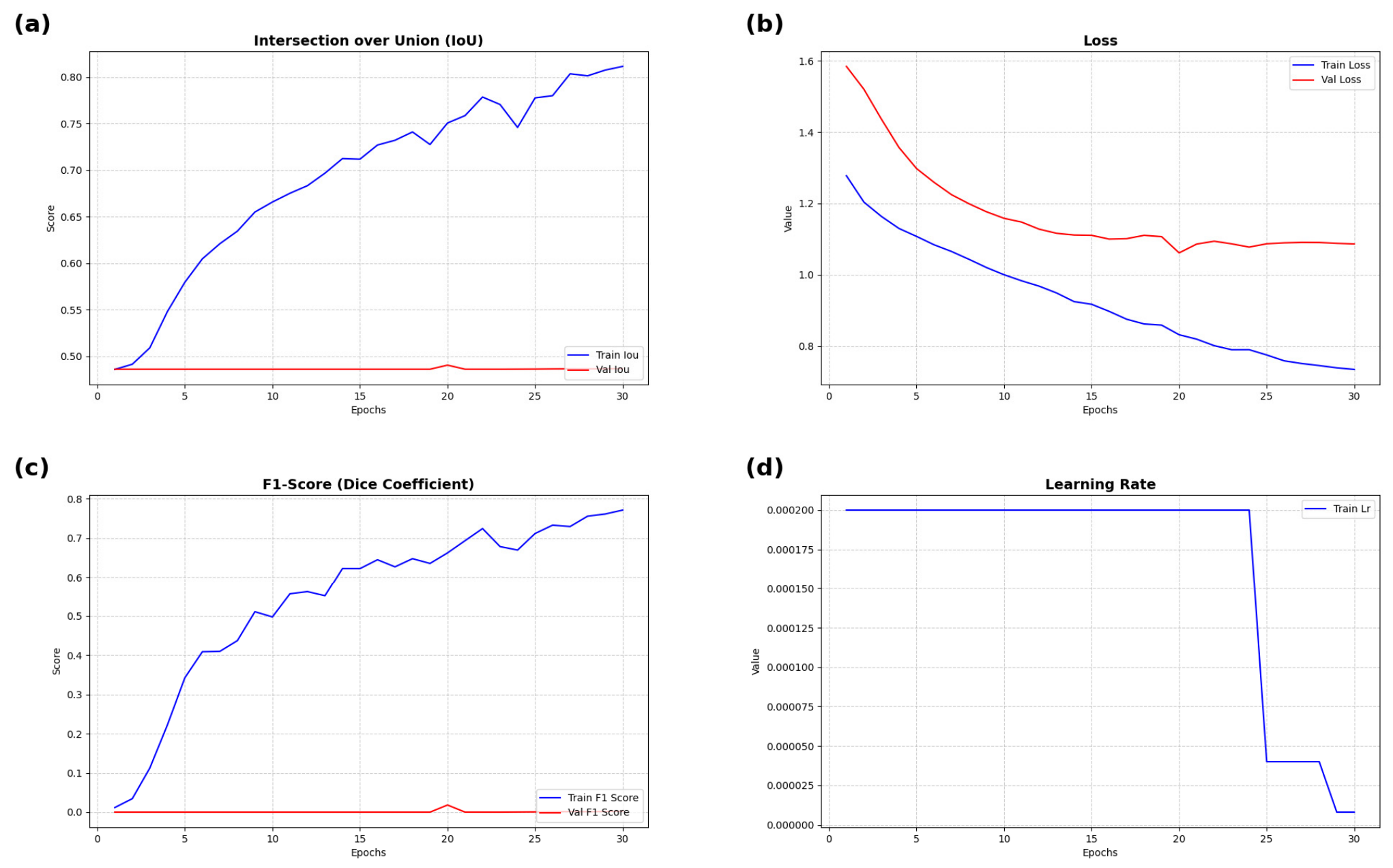
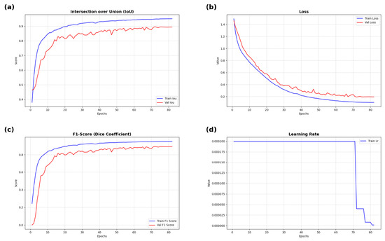
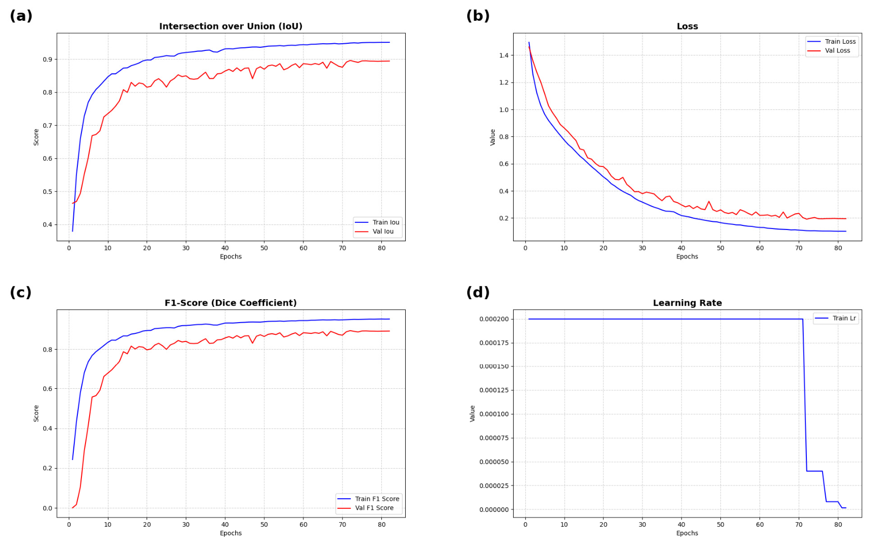
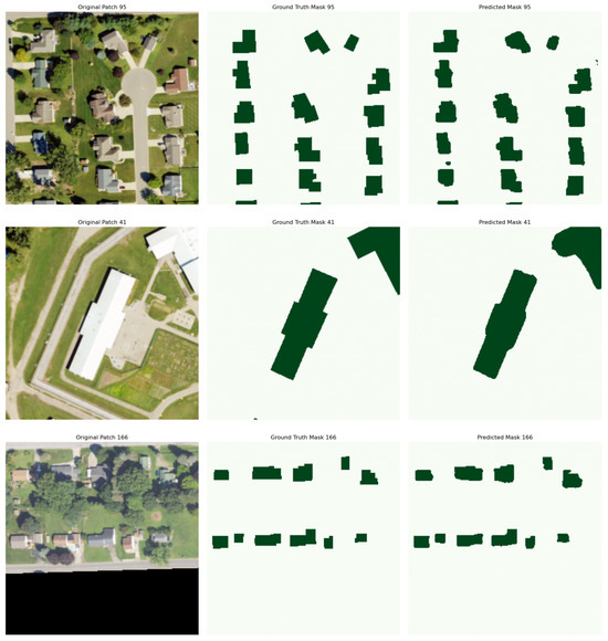
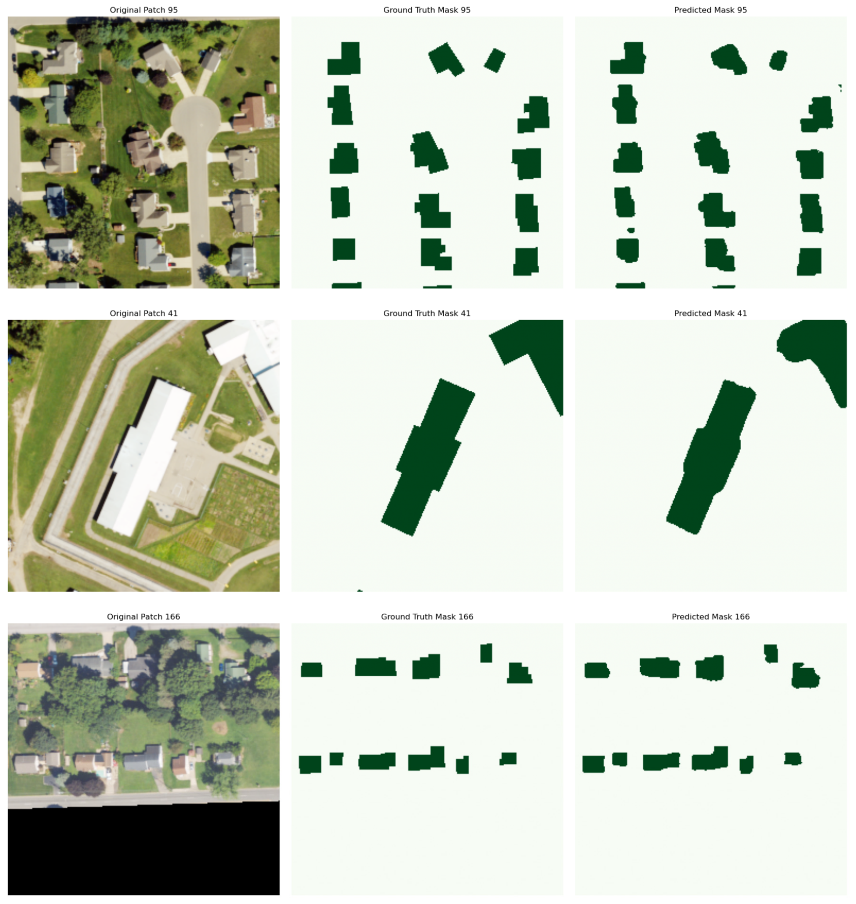
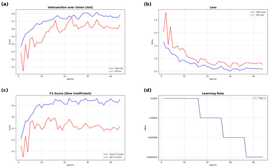
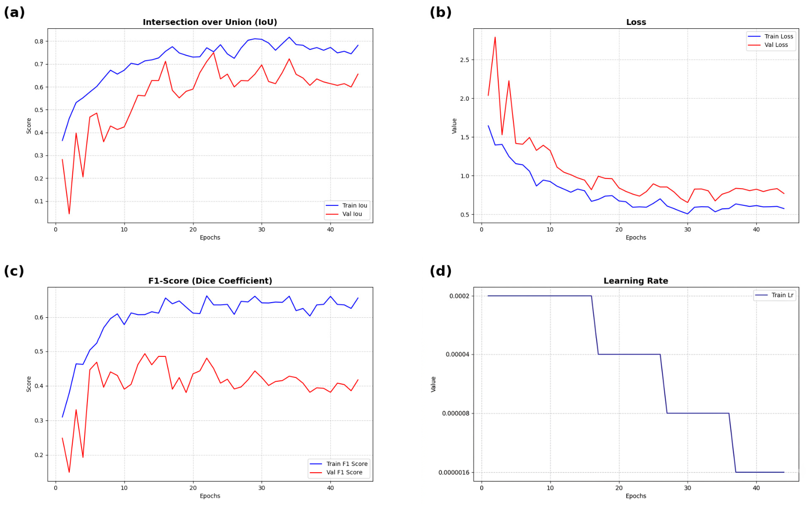
On the NAIP building dataset, in which buildings cover only a small part of each scene, the differences between the strategies were largest (Figure 11, Figure 12 and Figure 13). Sliding-window sampling (Figure 11) converged slowly and reached a validation IoU of 0.700 and an F1-score of 0.567. Random sampling (Figure 12) effectively failed: the validation F1-score remained close to zero (0.018), and the IoU stayed at 0.490, which shows that most randomly sampled patches contained no building pixels and the model learned to predict background almost everywhere. Object-centric sampling (Figure 13) reached an IoU of 0.896 and an F1-score of 0.894, as reported in

Table 2. Segmentation performance on NAIP validation dataset.

Sampling Strategy	IoU	Dice + BCE Loss	F1-Score	Epoch	Dataset Size	Training Time (min)
Sliding-window sampling	0.6997	0.8092	0.5666	100	629	109.78
Random sampling	0.4904	1.0612	0.0181	30	600	31.31
Object-centric sampling	0.8960	0.1909	0.8936	82	1728	242.8

, corresponding to gains of 19.6 percentage points in IoU and 32.7 percentage points in F1-score over sliding-window sampling. Because every patch was anchored to an annotated building, this strategy also produced the largest training set for this dataset (1728 patches). A qualitative comparison is shown in Figure 14, where individual buildings are delineated and correctly separated, even in the sparse suburban scenes.

3.3. UAV Water Body Segmentation

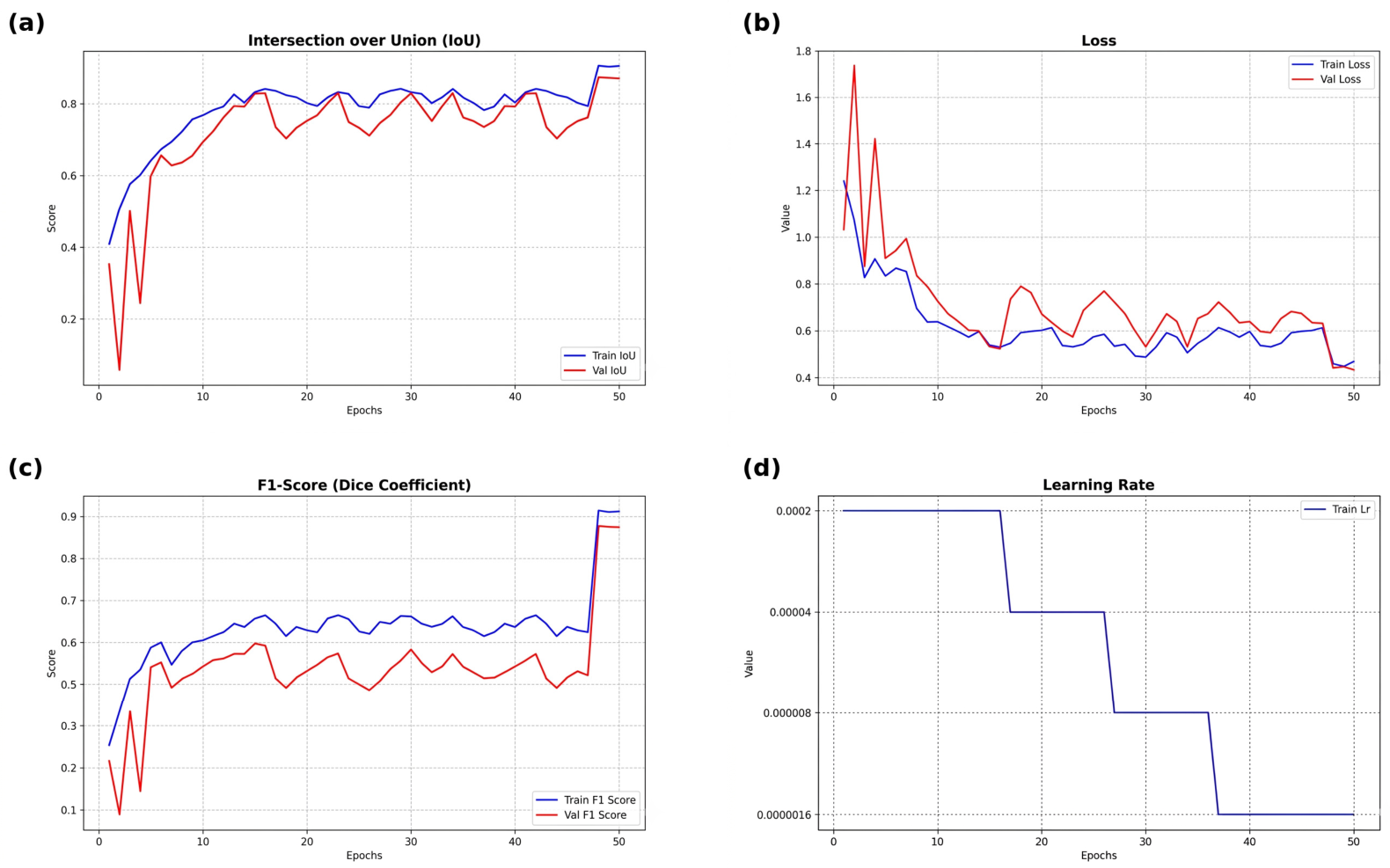
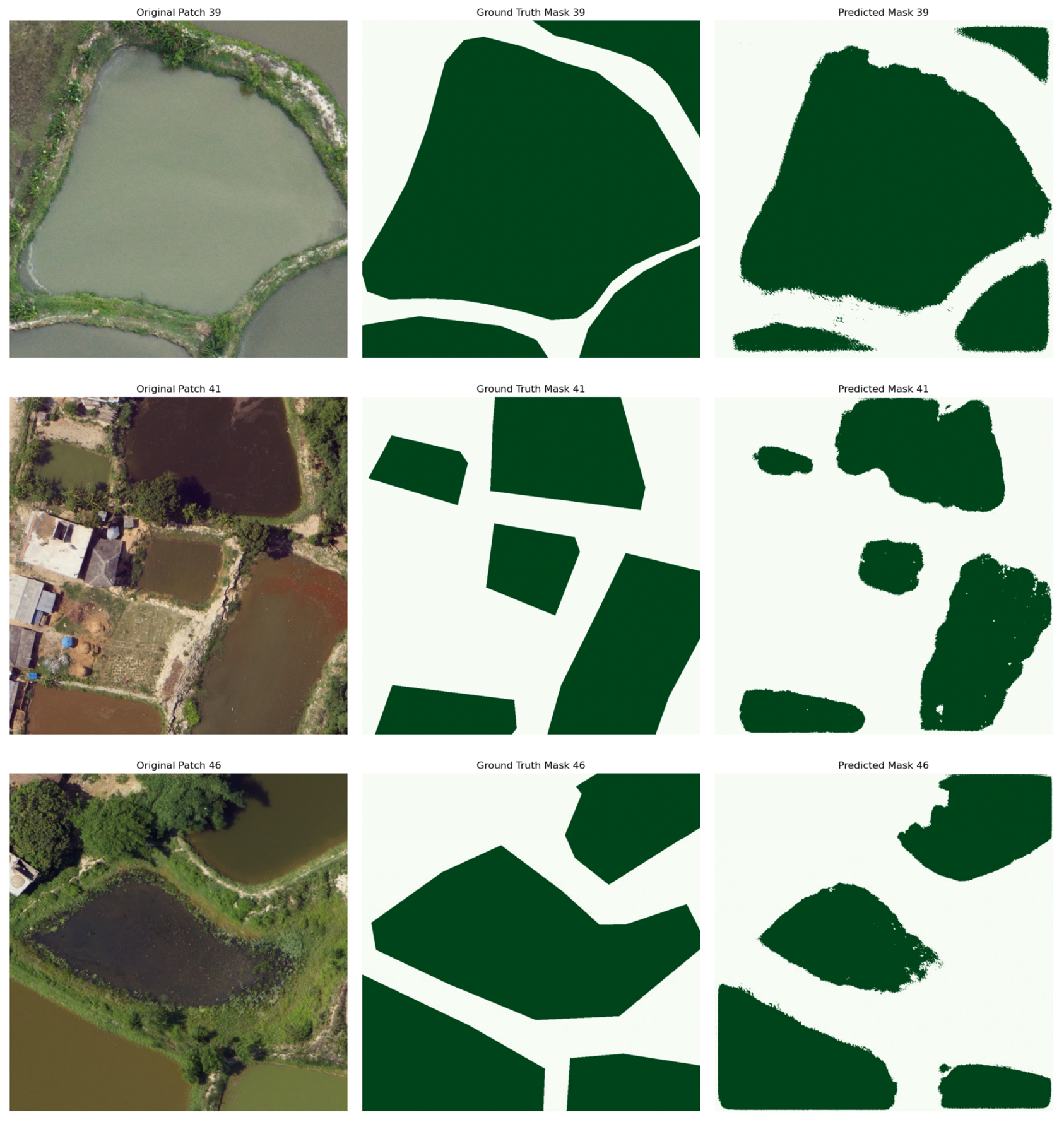
On the high-resolution UAV water body dataset, all three strategies achieved comparatively high accuracy because water bodies are visually distinct and occupy a large portion of each scene (Figure 15, Figure 16 and Figure 17). With sliding-window sampling (Figure 15) and random sampling (Figure 16), the validation curves were less stable than those produced by object-centric sampling (Figure 17). Object-centric sampling again gave the best result (IoU 0.912, F1-score 0.918), ahead of sliding-window sampling (IoU 0.884, F1-score 0.887) and random sampling (IoU 0.789, F1-score 0.784), as summarized in

Table 3. Segmentation performance on high-resolution UAV dataset.

Sampling Strategy	IoU	Dice + BCE Loss	F1-Score	Epoch	Dataset Size	Training Time (min)
Sliding-window sampling	0.884	0.628	0.887	52	1508	2038.823
Random sampling	0.789	0.751	0.784	47	782	1045.661
Object-centric sampling	0.9121	0.5475	0.9181	50	782	1038.429

. The very high spatial resolution required a larger patch size of 1024 × 1024 pixels, so the absolute training times were longer for all strategies; object-centric sampling nonetheless reached its accuracy from 782 patches, about half the 1508 patches used by sliding-window sampling, and in roughly half the training time (1038 min versus 2039 min). A qualitative comparison is shown in Figure 18, where the overall extent and shape of each water body are recovered, although the predicted boundaries appear slightly softer in places.

3.4. Multi-Model and Multi-Class Segmentation Validation

The evaluation was extended to the DeepLabV3+ architecture, equipped with an ImageNet-pretrained ResNet-50 backbone [24], to test whether the results depend on the choice of network. Using object-centric patch sets, DeepLabV3+ was trained under two distinct operational settings: (1) single-class target extraction (agricultural cotton fields) to verify cross-architecture generalizability against U-Net and (2) multi-class joint semantic segmentation (K = 3) containing co-occurring target classes (cotton and water) alongside background.

3.4.1. Cross-Architecture Validation (DeepLabV3+ vs. U-Net)

When trained on the object-centric Sentinel-2 cotton dataset (1597 patches), DeepLabV3+ achieved an IoU of 0.9297 and an F1-score of 0.9633 (

Table 4. Segmentation performance of DeepLabV3+ using object-centric patch sampling across single-class and multi-class configurations.

Task Complexity	Sampling Strategy	mIoU/IoU	Dice + BCE Loss	F1-Score
Single-class (cotton only)	U-Net (baseline)	0.9285	0.3207	0.9488
Single-class (cotton only)	DeepLabV3+	0.9297	0.2065	0.9633
Multi-class (cotton + water)	DeepLabV3+	0.9504	0.0725	0.9772

). Compared to the baseline U-Net model trained on the same object-centric patches (IoU 0.9285, F1-score 0.9488), DeepLabV3+ performed slightly better. This may reflect its Atrous Spatial Pyramid Pooling (ASPP) module, which aggregates multi-scale context and can make use of the higher target density of object-centric crops.

Convergence was stable, and training completed in 114.5 min. The learning curves for this configuration are shown in Figure 19. The gains from object-centric sampling are therefore not confined to encoder–decoder structures such as U-Net but also appear in a deeper architecture based on dilated convolutions.

3.4.2. Multi-Class Joint Segmentation

DeepLabV3+ was also trained on a multi-class dataset generated entirely by object-centric sampling, in which cotton and water occur within the same scene. Patches were extracted by anchoring crops to the cotton and water geometries in turn, supplemented by a 20% pure background allocation (4045 patches in total).

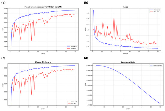
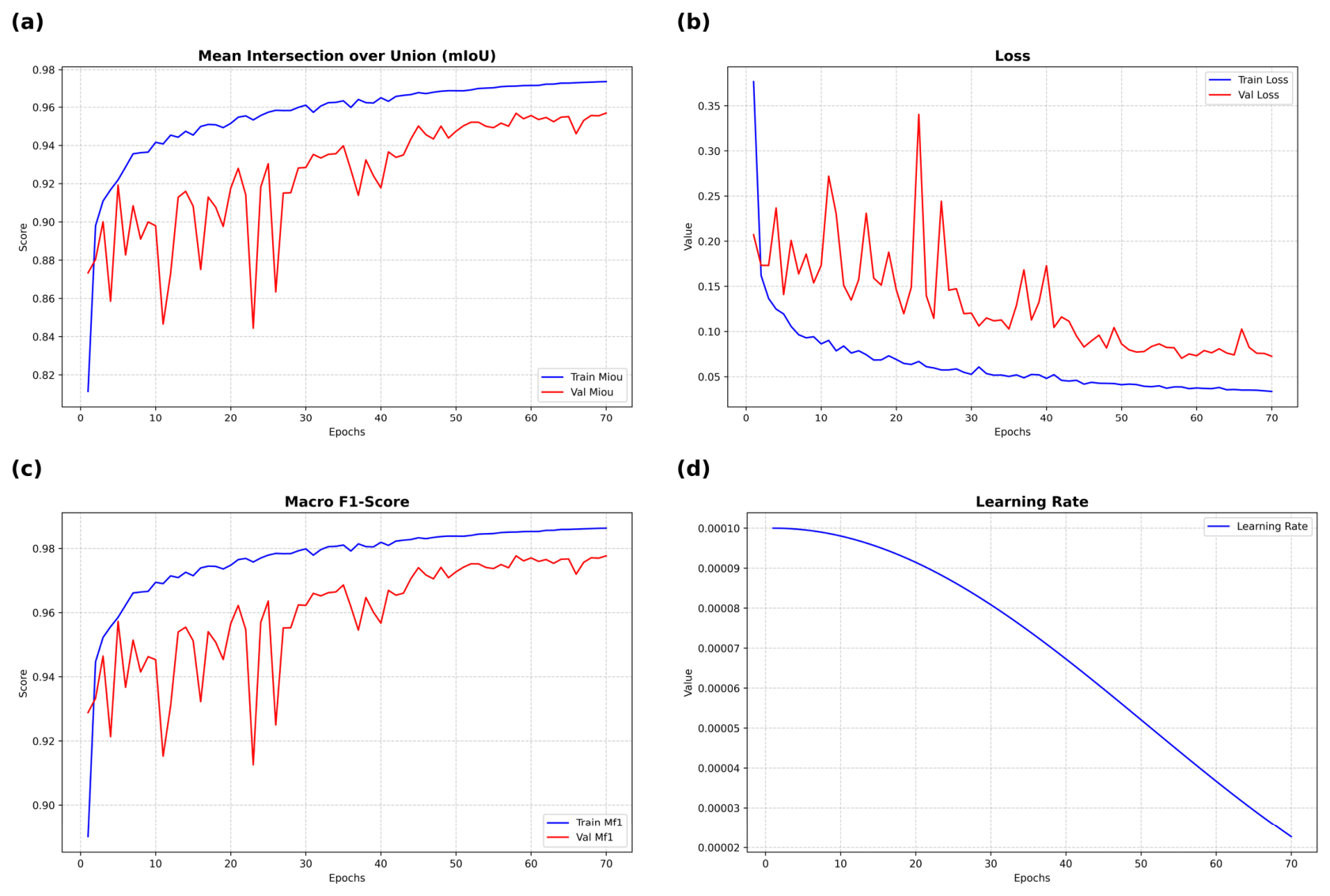
As summarized in Table 4, the multi-class DeepLabV3+ model achieved a mean IoU (mIoU) of 0.9504 and a mean F1-score of 0.9772 across all classes, reaching convergence in 142.2 min. The corresponding learning curves are shown in Figure 20. Class-specific values were an IoU of 0.9602 for cotton fields and 0.9406 for water bodies. Because object-centric sampling removes the background dominance typical of sliding-window crops, the class composition of each training batch was more balanced. In the qualitative results (Figure 21), boundaries between adjacent classes are delineated without visible confusion between the two target classes.

4. Discussion

The experimental results confirm that object-centric patch sampling consistently outperforms both sliding-window and random sampling across all three datasets. This improvement is not coincidental; conventional strategies prioritize patch volume over patch quality, producing background-dominated datasets and exposing the model to unlabeled objects that generate false-negative supervision [19,41,42], both of which corrupt model learning before any architectural decision is made. The failure of random sampling on the NAIP dataset further illustrates the severity of these problems under extreme class sparsity.

The magnitude of the improvement was closely related to the sparsity of the target class. The gain was largest for the NAIP building dataset, where buildings occupy only a small fraction of each scene, and smallest for the UAV water body dataset, where the targets are large and visually distinct. This pattern indicates that object-centric sampling is most valuable precisely under the conditions that are most difficult for conventional sampling, namely, sparse objects and incomplete annotation, while it remains at least as effective as conventional sampling when the target class is abundant.

By anchoring every patch to a confirmed annotated object, the proposed method directly improves the semantic quality of the training dataset. The 20% background allocation described in Section 2.3.5 allows the model to learn contextual background variability without diluting the object-centric character of the dataset.

The experiments also revealed an important limitation related to visually similar surface materials in high-resolution imagery. In some cases, the segmentation model incorrectly classified bitumen roads as buildings due to similarities in spectral response and texture patterns. Since semantic segmentation operates at the pixel level, such confusion can occur when contextual object-level understanding is limited. A promising direction for future research is therefore the integration of an object detection stage before segmentation. In this framework, an object detection model could first identify probable building candidate regions, and only those regions would subsequently be passed to the segmentation model for precise boundary extraction. Such a hybrid detection-segmentation pipeline could reduce false positives caused by road surfaces and further improve segmentation reliability in complex urban environments.

Unlike focal loss [21] or class reweighting [12], which attempt to compensate for imbalance during optimization, the proposed method addresses the problem at the data construction stage itself, without modifying the model architecture, loss function, or training procedure. Training time differences across datasets mainly reflect patch corpus size and early stopping convergence behavior rather than a simple computational efficiency trade-off and are therefore reported alongside epoch counts in Table 1, Table 2 and Table 3 for transparency. The primary limitation of the proposed method remains its dependence on existing annotations; in scenarios with near-zero label coverage, the strategy gradually degenerates toward random sampling behavior. In addition, the present evaluation is restricted to convolutional architectures, which should be borne in mind when generalizing the results.

A further distinction should be drawn between the multi-class setting evaluated here and full-class semantic segmentation. The classes used in Section 3.4.2 are discrete and individually delineated, so each carries a geometric centroid that can serve as an anchor. In full-class parsing, every pixel is assigned to some category, and categories such as grassland, forest, or built-up background appear as continuous regions rather than separate objects. A centroid computed over such a region is not a useful sampling anchor, since a single point cannot represent an extended and often irregular area, and for concave regions it may fall outside the region itself. The problems that object-centric sampling is designed to remove also change character here because when annotation is exhaustive, there are no background-only patches to discard and no unlabeled objects to generate false-negative supervision. Extending the method to this setting would therefore require a different anchoring rule, such as placing anchors on class boundaries located from the spatial gradient of the multi-class mask, so that patches concentrate where categories meet and misclassification is most frequent. This possibility has not been tested here and is left for future work.

Finally, while object-centric patch sampling offers efficiency and accuracy gains for sparse object distributions, its advantages diminish in scenes dominated by contiguous, high-density land cover or in workflows lacking prior vector annotations, where non-overlapping sliding windows remain practical. Nevertheless, for target-focused remote sensing applications, anchoring patch extraction directly to vector centroids provides a data-centric approach that removes uninformative background and reduces false-negative supervision, giving higher segmentation performance without changes to model architectures, loss functions, or training routines.

5. Conclusions

This study demonstrated that data quality, not data quantity, is the decisive factor in patch-based deep learning for remote sensing segmentation. By anchoring training patches to annotated object centroids, the proposed object-centric sampling strategy guarantees that every training sample carries meaningful target information, eliminates background-only patches, and avoids label-missing regions that generate false-negative supervision, thereby addressing the root causes of class imbalance and negative learning at the data construction stage rather than through model-level compensation. Evaluated across satellite, aerial, and UAV imagery spanning three segmentation tasks and two network architectures, the method consistently achieved the highest IoU and F1-scores in all configurations, outperforming sliding-window and random sampling without any modification to model architecture, loss function, or training procedure. Unlike existing mitigation strategies such as focal loss or class reweighting, which operate downstream of a fundamentally flawed training set, object-centric sampling improves the training data itself, making it a simple, model-independent, and universally applicable first step in any remote sensing deep learning pipeline. These findings indicate that patch sampling should be regarded as an explicit design decision rather than a routine preprocessing step, particularly when the target class is sparse or the annotations are incomplete. Future work will explore its extension to semi-supervised annotation settings and transformer-based architectures.

References

- Krejcar, O.; Namazi, H. AI in Remote Sensing and Satellite Image Processing—A Review. Environ. Earth Sci. 2026, 85, 78. [Google Scholar] [CrossRef] [Scilit]
- Lu, W.; Shi, X.; Lu, Z. A New Two-Step Road Extraction Method in High Resolution Remote Sensing Images. PLoS ONE 2024, 19, e0305933. [Google Scholar] [CrossRef] [Scilit] [PubMed]
- Zhu, X.; Cai, F.; Tian, J.; Williams, T.K.-A. Spatiotemporal Fusion of Multisource Remote Sensing Data: Literature Survey, Taxonomy, Principles, Applications, and Future Directions. Remote Sens. 2018, 10, 527. [Google Scholar] [CrossRef] [Scilit]
- Liu, Q.; Huang, T.; Dong, Y.; Yang, J.; Xiang, W. From Pixels to Images: Deep Learning Advances in Remote Sensing Image Semantic Segmentation. arXiv 2025, arXiv:2505.15147. [Google Scholar] [CrossRef] [Scilit]
- Ji, S.; Wei, S.; Lu, M. Fully Convolutional Networks for Multisource Building Extraction from an Open Aerial and Satellite Imagery Data Set. IEEE Trans. Geosci. Remote Sens. 2019, 57, 574–586. [Google Scholar] [CrossRef] [Scilit]
- Silwal, A.; Subedi, A.; Tamrakar, R.; Dahal, K.; Dahal, D.; Ekpetere, K.O.; Zhran, M. A Comprehensive Review of Machine Learning and Deep Learning Methods for Flood Inundation Mapping. Earth 2026, 7, 44. [Google Scholar] [CrossRef] [Scilit]
- Cao, H.; Tian, Y.; Liu, Y.; Wang, R. Water Body Extraction from High Spatial Resolution Remote Sensing Images Based on Enhanced U-Net and Multi-Scale Information Fusion. Sci. Rep. 2024, 14, 16132. [Google Scholar] [CrossRef] [Scilit] [PubMed]
- Zhang, P.; Ke, Y.; Zhang, Z.; Wang, M.; Li, P.; Zhang, S. Urban Land Use and Land Cover Classification Using Novel Deep Learning Models Based on High Spatial Resolution Satellite Imagery. Sensors 2018, 18, 3717. [Google Scholar] [CrossRef] [Scilit] [PubMed]
- Ronneberger, O.; Fischer, P.; Brox, T. U-Net: Convolutional Networks for Biomedical Image Segmentation. In Medical Image Computing and Computer-Assisted Intervention—MICCAI 2015; Navab, N., Hornegger, J., Wells, W.M., Frangi, A.F., Eds.; Lecture Notes in Computer Science; Springer: Cham, Switzerland, 2015; Volume 9351, pp. 234–241. [Google Scholar] [CrossRef] [Scilit]
- Lian, R.; Huang, L. DeepWindow: Sliding Window Based on Deep Learning for Road Extraction from Remote Sensing Images. IEEE J. Sel. Top. Appl. Earth Obs. Remote Sens. 2020, 13, 1905–1916. [Google Scholar] [CrossRef] [Scilit]
- Siva, S.S.; Cross-Zamirski, J.O. Building Damage Detection Using Satellite Images and Patch-Based Transformer Methods. arXiv 2026, arXiv:2602.08117. [Google Scholar] [CrossRef] [Scilit]
- Buda, M.; Maki, A.; Mazurowski, M.A. A Systematic Study of the Class Imbalance Problem in Convolutional Neural Networks. Neural Netw. 2018, 106, 249–259. [Google Scholar] [CrossRef] [Scilit] [PubMed]
- Xia, W.; Ma, C.; Liu, J.; Liu, S.; Chen, F.; Yang, Z.; Duan, J. High-Resolution Remote Sensing Imagery Classification of Imbalanced Data Using Multistage Sampling Method and Deep Neural Networks. Remote Sens. 2019, 11, 2523. [Google Scholar] [CrossRef] [Scilit]
- Zhou, Z.; Zheng, C.; Liu, X.; Tian, Y.; Chen, X.; Chen, X.; Dong, Z. A Dynamic Effective Class Balanced Approach for Remote Sensing Imagery Semantic Segmentation of Imbalanced Data. Remote Sens. 2023, 15, 1768. [Google Scholar] [CrossRef] [Scilit]
- Garcia-Garcia, A.; Orts-Escolano, S.; Oprea, S.; Villena-Martinez, V.; Martinez-Gonzalez, P.; Garcia-Rodriguez, J. A Survey on Deep Learning Techniques for Image and Video Semantic Segmentation. Appl. Soft Comput. 2018, 70, 41–65. [Google Scholar] [CrossRef] [Scilit]
- Zhu, X.X.; Tuia, D.; Mou, L.; Xia, G.-S.; Zhang, L.; Xu, F.; Fraundorfer, F. Deep Learning in Remote Sensing: A Comprehensive Review and List of Resources. IEEE Geosci. Remote Sens. Mag. 2017, 5, 8–36. [Google Scholar] [CrossRef] [Scilit]
- Rolnick, D.; Veit, A.; Belongie, S.; Shavit, N. Deep Learning Is Robust to Massive Label Noise. arXiv 2018, arXiv:1705.10694. [Google Scholar] [CrossRef] [Scilit]
- Northcutt, C.G.; Jiang, L.; Chuang, I.L. Confident Learning: Estimating Uncertainty in Dataset Labels. J. Artif. Intell. Res. 2021, 70, 1373–1411. [Google Scholar] [CrossRef] [Scilit]
- Kim, Y.; Yim, J.; Yun, J.; Kim, J. NLNL: Negative Learning for Noisy Labels. In Proceedings of the 2019 IEEE/CVF International Conference on Computer Vision (ICCV), Seoul, Republic of Korea, 27 October–2 November 2019; pp. 101–110. [Google Scholar] [CrossRef] [Scilit]
- Roth, K.; Milbich, T.; Sinha, S.; Gupta, P.; Ommer, B.; Cohen, J.P. Revisiting Training Strategies and Generalization Performance in Deep Metric Learning. In Proceedings of the 37th International Conference on Machine Learning (ICML 2020), Virtual, 13–18 July 2020; Proceedings of Machine Learning Research; PMLR: Cambridge, MA, USA, 2020; Volume 119, pp. 8242–8252. Available online: https://proceedings.mlr.press/v119/roth20a.html (accessed on 4 August 2026).
- Lin, T.-Y.; Goyal, P.; Girshick, R.; He, K.; Dollár, P. Focal Loss for Dense Object Detection. In Proceedings of the 2017 IEEE International Conference on Computer Vision (ICCV), Venice, Italy, 22–29 October 2017; pp. 2999–3007. [Google Scholar] [CrossRef] [Scilit]
- He, H.; Garcia, E.A. Learning from Imbalanced Data. IEEE Trans. Knowl. Data Eng. 2009, 21, 1263–1284. [Google Scholar] [CrossRef] [Scilit]
- Liu, C.; Albrecht, C.M.; Wang, Y.; Zhu, X.X. AIO2: Online Correction of Object Labels for Deep Learning with Incomplete Annotation in Remote Sensing Image Segmentation. IEEE Trans. Geosci. Remote Sens. 2024, 62, 5613917. [Google Scholar] [CrossRef] [Scilit]
- Chen, L.-C.; Zhu, Y.; Papandreou, G.; Schroff, F.; Adam, H. Encoder-decoder with atrous separable convolution for semantic image segmentation. In Proceedings of the European Conference on Computer Vision (ECCV), Munich, Germany, 8–14 September 2018; pp. 801–818. [Google Scholar]
- Dalal, N.; Triggs, B. Histograms of Oriented Gradients for Human Detection. In Proceedings of the 2005 IEEE Computer Society Conference on Computer Vision and Pattern Recognition (CVPR), San Diego, CA, USA, 20–25 June 2005; IEEE: Piscataway, NJ, USA, 2005; Volume 1, pp. 886–893. [Google Scholar] [CrossRef] [Scilit]
- Jarrahi, M.H.; Memariani, A.; Guha, S. The Principles of Data-Centric AI. Commun. ACM 2023, 66, 84–92. [Google Scholar] [CrossRef] [Scilit] [PubMed]
- Bengio, Y. Practical Recommendations for Gradient-Based Training of Deep Architectures. In Neural Networks: Tricks of the Trade; Montavon, G., Orr, G.B., Müller, K.-R., Eds.; Springer: Berlin/Heidelberg, Germany, 2012; Volume 7700, pp. 437–478. [Google Scholar] [CrossRef] [Scilit]
- Ren, P.; Xiao, Y.; Chang, X.; Huang, P.-Y.; Li, Z.; Gupta, B.B.; Chen, X.; Wang, X. A Survey of Deep Active Learning. ACM Comput. Surv. 2021, 54, 1–40. [Google Scholar] [CrossRef] [Scilit]
- MMSegmentation Contributors. MMSegmentation: OpenMMLab Semantic Segmentation Toolbox and Benchmark. Available online: https://github.com/open-mmlab/mmsegmentation (accessed on 15 August 2026).
- Kaiser, P.; Wegner, J.D.; Lucchi, A.; Jaggi, M.; Hofmann, T.; Schindler, K. Learning Aerial Image Segmentation from Online Maps. IEEE Trans. Geosci. Remote Sens. 2017, 55, 6054–6068. [Google Scholar] [CrossRef] [Scilit]
- Goodfellow, I.; Bengio, Y.; Courville, A. Deep Learning; MIT Press: Cambridge, MA, USA, 2016. [Google Scholar]
- Braden, B. The Surveyor’s Area Formula. Coll. Math. J. 1986, 17, 326–337. [Google Scholar] [CrossRef]
- Preparata, F.P.; Shamos, M.I. Computational Geometry: An Introduction; Springer: New York, NY, USA, 1985. [Google Scholar] [CrossRef] [Scilit]
- Rouault, E.; Warmerdam, F.; Schwehr, K.; Kiselev, A.; Butler, H.; Łoskot, M.; Szekeres, T.; Tourigny, E.; Landa, M.; Miara, I.; et al. GDAL, version 3.13.0; Zenodo: Geneva, Switzerland, 2026. [Google Scholar] [CrossRef]
- Drusch, M.; Del Bello, U.; Carlier, S.; Colin, O.; Fernandez, V.; Gascon, F.; Hoersch, B.; Isola, C.; Laberinti, P.; Martimort, P.; et al. Sentinel-2: ESA’s Optical High-Resolution Mission for GMES Operational Services. Remote Sens. Environ. 2012, 120, 25–36. [Google Scholar] [CrossRef] [Scilit]
- Schroeder, T.A.; Obata, S.; Papeş, M.; Branoff, B. Evaluating Statewide NAIP Photogrammetric Point Clouds for Operational Improvement of National Forest Inventory Estimates in Mixed Hardwood Forests of the Southeastern U.S. Remote Sens. 2022, 14, 4386. [Google Scholar] [CrossRef] [Scilit]
- Kingma, D.P.; Ba, J. Adam: A Method for Stochastic Optimization. In Proceedings of the 3rd International Conference on Learning Representations (ICLR 2015), San Diego, CA, USA, 7–9 May 2015. [Google Scholar] [CrossRef] [Scilit]
- Prechelt, L. Early Stopping—But When? In Neural Networks: Tricks of the Trade; Orr, G.B., Müller, K.-R., Eds.; Lecture Notes in Computer Science; Springer: Berlin/Heidelberg, Germany, 1998; Volume 1524, pp. 55–69. [Google Scholar] [CrossRef] [Scilit] [PubMed]
- Milletari, F.; Navab, N.; Ahmadi, S.-A. V-Net: Fully Convolutional Neural Networks for Volumetric Medical Image Segmentation. In Proceedings of the 2016 Fourth International Conference on 3D Vision (3DV), Stanford, CA, USA, 25–28 October 2016; pp. 565–571. [Google Scholar] [CrossRef] [Scilit]
- Everingham, M.; Van Gool, L.; Williams, C.K.I.; Winn, J.; Zisserman, A. The PASCAL Visual Object Classes (VOC) Challenge. Int. J. Comput. Vis. 2010, 88, 303–338. [Google Scholar] [CrossRef] [Scilit]
- Rolnick, D.; Donti, P.L.; Kaack, L.H.; Kochanski, K.; Lacoste, A.; Sankaran, K.; Ross, A.S.; Milojevic-Dupont, N.; Jaques, N.; Waldman-Brown, A.; et al. Tackling Climate Change with Machine Learning. ACM Comput. Surv. 2022, 55, 42. [Google Scholar] [CrossRef] [Scilit]
- Xiao, Y.; Zhao, Y.; Shu, K. Understanding and Tackling Label Errors in Individual-Level Nature Language Understanding. arXiv 2025, arXiv:2502.13297. [Google Scholar] [CrossRef] [Scilit]
Disclaimer/Publisher’s Note: The statements, opinions and data contained in all publications are solely those of the individual author(s) and contributor(s) and not of MDPI and/or the editor(s). MDPI and/or the editor(s) disclaim responsibility for any injury to people or property resulting from any ideas, methods, instructions or products referred to in the content. |
© 2026 by the authors. Licensee MDPI, Basel, Switzerland. This article is an open access article distributed under the terms and conditions of the Creative Commons Attribution (CC BY) license.