


Highlights
What are the main findings?
- Classifier-shared class semantic prototype enables task-oriented aggregation, fusion, and cyclic refinement of complementary HSI and LiDAR features.
- Extensive experiments on the Houston2013, Trento and MUUFL datasets demonstrate the consistent superiority and general effectiveness of CSPGFNet.
What are the implications of the main findings?
- Class semantic prototype provides an effective bridge for directly aligning heterogeneous multimodal interactions with the final classification objective.
- The proposed framework offers a promising strategy for exploiting complementary spectral–spatial–elevation information in multimodal remote sensing classification.
Abstract
Benefiting from information complementarity, the fusion of hyperspectral imagery (HSI) and light detection and ranging (LiDAR) data for land cover classification has attracted significant attention in the remote sensing community. However, due to modality imbalance and information redundancy, effectively extracting and integrating complementary knowledge from HSI and LiDAR data remains a major challenge. To address the aforementioned issues, a class semantic prototype guided fusion network (CSPGFNet) is proposed to realize efficient and accurate classification by task-relevant feature mining, fusion, and interaction. Specifically, feature extraction sub-networks with multi-scale and multi-type convolutional structures are designed for each modality to mitigate semantic imbalance caused by inherent dimensional discrepancies. Moreover, a feature fusion-interaction module based on cross-attention mechanism is designed to fuse and interact task-relevant spatial–spectral and elevation information from modalities with class semantic prototype (CSP) as the bridge. Furthermore, a composite loss that incorporates multi-factor constraints is optimized to ensure information complementarity, semantic consistency and task relevance of the whole network. Experimental evaluations on three benchmark datasets demonstrate the effectiveness of the proposed method.
1. Introduction
The emergence of multimodal fusion techniques is fundamentally advancing the paradigm of remote sensing analysis, overcoming the inherent limitations of single-modal data in providing a comprehensive characterization of the Earth’s surface [1,2,3,4]. Among various sensor combinations, the integration of HSI and LiDAR stands out as a particularly promising and complementary strategy [5,6]. While HSI captures detailed spectral response that enables the discrimination of subtle material variances, LiDAR accurately records the elevation of targets [7,8,9]. This inherent complementarity offers unprecedented opportunities to synergistically leverage both spectral and spatial structural attributes, thereby facilitating a more accurate and robust interpretation of land covers [10,11]. By combining these complementary strengths, the fusion of HSI and LiDAR offers great potential for a wide range of fine-scale applications, including urban mapping [12], vegetation monitoring [13,14], and material-level classification [15,16], where single-modality observations often fall short [17,18]. However, realizing this potential is non-trivial, as HSI and LiDAR, being heterogeneous sources, exhibit significant differences in both imaging principles and information characteristics, making the design of effective feature fusion strategies a critical issue.
More specifically, the cross-modal representation imbalance considered in this study refers to the unequal richness and discriminative capacity of modality-specific features caused by substantial differences in input dimensionality and information content between HSI and LiDAR. The abundant spectral information of HSI may dominate feature learning and fusion, leaving the structural and elevation cues provided by LiDAR insufficiently represented. Meanwhile, information redundancy refers to overlapping or highly correlated information retained across the two modality-specific representations, which may dilute their complementary and task-relevant cues. Therefore, the central problem is how to balance the representational capacity of the two modalities while selectively integrating complementary information under a unified classification objective.
In the initial study, the substantial heterogeneity between HSI and LiDAR data led most methods to focus on feature-level fusion methods, where features extracted from each modality were independently optimized to better capture semantic representations before being integrated [19,20]. Convolutional neural networks (CNNs) as one of the mainstream methods in deep learning, have become the dominant feature extraction backbone in this category of methods [21,22]. Hong et al. [23] proposed a baseline solution to the multimodal fusion by developing a general multimodal deep learning framework, at the same time, the effects of different fusion strategies were compared. Wu et al. [24] used a dual-branch convolutional neural network to separately extract features from hyperspectral and LiDAR images, and then performed feature fusion along the channel dimension. Roy et al. [25] proposed a joint feature learning and fusion mechanism using CNNs and spatial morphology blocks for both HSI and LiDAR, which leverages distinct feature extraction methods tailored to each modality, enhancing the overall performance of the fusion process. A suite of modern deep learning modules such as attention mechanisms, generative adversarial networks (GANs), and graph convolutional networks (GCNs) have been increasingly integrated to complement feature extraction, enhancing discriminative power and modeling complex semantic structures [26,27]. Lu et al. [28] proposed a coupled adversarial learning based classification method to extract features from both modalities are encouraged to become more discriminative, reducing modality gaps and enhancing their contribution to the classification task. Ding et al. [29] designed a global–local transformer network to capture complex local and global spatial–spectral correlations between the two modalities. Although the aforementioned methods can capture and fuse features from different modalities, and improve the performance of land-cover classification, they perform feature extraction modality independently without cross-modal interaction, resulting in information redundancy. Moreover, these methods are often sensitive to outliers, restricting their effectiveness when dealing with large-scale and complex data.
With the development of deep learning, fusion strategies are no longer limited to feature-level operations, but have evolved to incorporate cross-modal information interaction across multiple stages to enhance the complementarity between HSI and LiDAR features [30,31]. The emergence of cross-attention mechanisms has provided effective means for fine-grained information exchange across modalities [32,33]. Wang et al. [34] developed a multi-attentive hierarchical fusion network that enables cross-modal interaction and fusion by exchanging attention maps during the attention computation process. Transformer provides an innovative paradigm for cross-modal information interaction through its global context modeling capability and dynamic interaction mechanism [35,36]. Roy et al. [37] introduced a multimodal fusion transformer that treated LiDAR images as classification tokens and integrated spectral features from HSI to achieve modality fusion. Zhao et al. [38] proposed a dual-branch framework that combines CNNs and transformer networks to fuse heterogeneous multi-source information and improve joint classification performance. Feng et al. [39] developed a spectral–spatial–elevation fusion transformer that leverages LiDAR-derived elevation information to guide spectral feature aggregation from hyperspectral imagery. More recent studies have shifted their focus from feature interaction to semantic-aware representation learning. For example, Song et al. [40] explicitly decomposed multimodal representations into common and modality-specific components to facilitate complementary information learning, while Ni et al. [41] progressively performed hierarchical cross-modal interaction to enhance semantic consistency across heterogeneous modalities. These methods substantially improve the capability of modeling complementary information between HSI and LiDAR. However, a semantic gap exists between their interaction mechanisms and the ultimate classification objective. Because this interaction lacks guidance from a high-level supervisory signal, there is no guarantee that the cross-modal information flow will be effectively translated into enhanced discriminative power, which consequently becomes a performance bottleneck in complex scenarios.
Despite these advances, existing HSI–LiDAR fusion methods still face two fundamental challenges. First, their heterogeneous dimensionality and information characteristics can cause cross-modal representational imbalance, defined here as the unequal ability of modality-specific features to encode and contribute task-relevant semantics, rather than class-distribution imbalance. The spectrally rich HSI may dominate joint learning, leaving complementary LiDAR elevation and structural cues underrepresented. Thus, dimensional discrepancy is an important source of this imbalance, while unequal task contributions are its manifestation. Second, existing interaction mechanisms often lack explicit guidance from the classification objective. Indiscriminate aggregation may repeatedly propagate shared or irrelevant responses, increasing redundancy rather than complementarity. Therefore, effective fusion should enhance underrepresented task-relevant information and guide cross-modal interaction toward complementary and class-discriminative representations.
These observations motivate the introduction of class semantic prototype as task-oriented references for cross-modal fusion. By sharing parameters with the final classifier, each prototype is directly optimized by the classification objective and is therefore encouraged to encode class-discriminative semantics. When used to guide cross-modal aggregation, these prototypes can selectively emphasize category-relevant spectral, spatial, and elevation cues while suppressing shared or task-irrelevant responses. Rather than directly eliminating the inherent dimensional discrepancy between HSI and LiDAR, prototype guidance is expected to reduce its adverse influence on feature fusion by enhancing the effective contribution of underrepresented complementary information. Consequently, it can promote task-relevant semantic alignment, reduce redundant feature overlap, and improve the discriminability of the fused representation.
Guided by this rationale, we propose a Class Semantic Prototype Guided Fusion Network (CSPGFNet). First, a modality-specific feature extraction module is developed to alleviate cross-modal representational imbalance. In particular, multi-scale convolutional operations are introduced into the relatively information-sparse LiDAR branch to enrich its structural representation, thereby preventing its elevation cues from being overwhelmed by the spectrally rich HSI features. Second, a class semantic prototype, whose parameters are shared with the final classifier, is employed as a task-oriented semantic bridge to guide cross-modal feature aggregation. This design enables the network to selectively extract class-relevant information from each modality rather than indiscriminately mixing all available features. Third, the prototype guided fused representation is converted back into the modality-specific feature spaces, forming a cyclic interaction process that allows each modality to absorb complementary information. Finally, semantic consistency and information complementarity constraints are introduced to align the fused representation with the classification objective while discouraging excessive similarity and redundancy between modality-specific features.
The main contributions of this study are summarized as follows:
- To mine and fuse the most complementary and useful features in HSI and LiDAR joint classification, we propose a class semantic prototype guided fusion framework, which aligns semantic features based on cross-attention and prototype guidance.
- To enable semantic-aligned fusion, we propose an information-sparse modality enhancement strategy, where a dedicated multi-scale convolutional structure is designed to balance feature expression and the CSP is used as the query to effectively aggregate and align features.
- To fully exploit inter-modal complementarity, we propose an inverse feature conversion mechanism that leverages the fusion features as keys and values, enabling each modality to distill complementary information back into its own representation, thereby forming a closed-loop of semantic interaction.
- To further enhance the fusion efficacy and reduce information redundancy, we incorporate a multi-factor loss constraint within the CSP guided semantic space, which promotes feature complementarity and establishes coherent semantic fusion space to ensure a highly effective fused feature.
The remainder of this paper is organized as follows. Section 2 presents the proposed CSPGFNet. Section 3 introduces the datasets and implementation details. Section 4 reports the comparative and ablation experiments. Section 5 discusses parameter sensitivity, computational complexity, feature representations, and limitations. Finally, Section 6 concludes this study.
2. Methodology
2.1. Overall Architecture
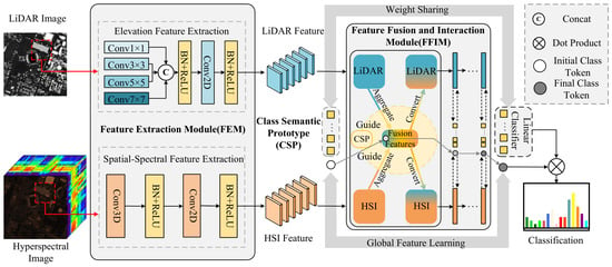
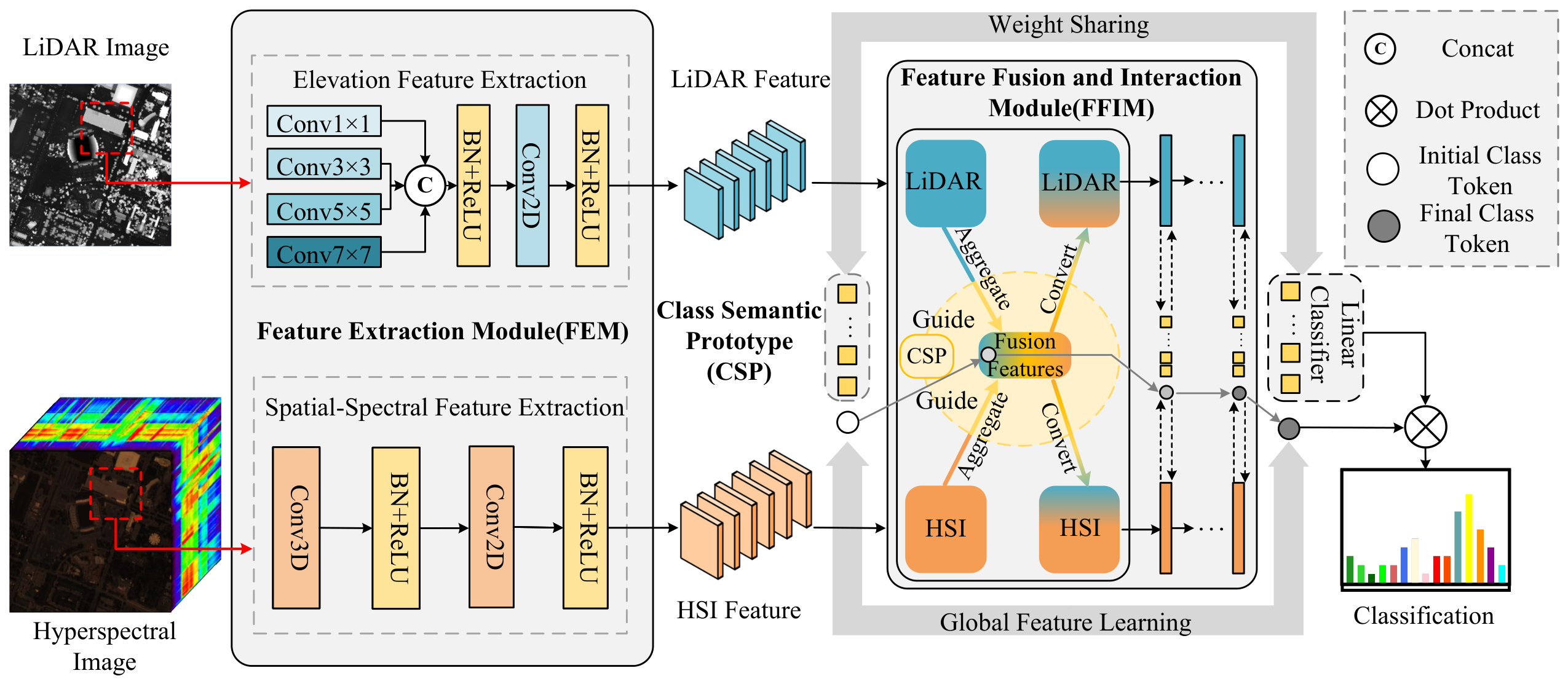
In this article, we propose a CSPGFNet for the HSI and LiDAR data classification, which employs CSP as the bridge and integrates a cross-attention mechanism with multiple loss constraints to achieve complementary interaction and efficient fusion of task-relevant features across modalities. As illustrated in Figure 1, the proposed model consists of three main parts: feature extraction module, feature fusion and interaction module, and objective function. Specifically, the feature extraction module aims to alleviate cross-modal representational imbalance by learning modality-aware representations. The feature fusion and interaction module establishes a semantic bridge between HSI and LiDAR through CSP-guided cross-attention, enabling selective aggregation and bidirectional interaction of task-relevant information. The objective function further constrains the learned representations from the perspectives of classification, semantic consistency, and information complementarity. The framework follows a coherent data flow: the input HSI and LiDAR data are first processed through the feature extraction module to generate balanced feature representations for both modalities. These refined features are then fed into the CSP guided fusion and interaction module, where they undergo iterative optimization through cross-attention. During this process, a classification token is incorporated to learn and integrate modal-specific characteristics, ultimately producing a discriminative fused representation for the final classification task. The subsequent sections will detail each component of the framework.
Figure 1.
Overall architecture of the proposed network for HSI and LiDAR fusion and classification. The feature extraction module employs modality-specific branches to extract multi-scale LiDAR elevation features and HSI spatial–spectral features. The extracted representations are iteratively aggregated, fused, and updated in the feature fusion and interaction module under the guidance of classifier-coupled class semantic prototypes. A classification token collects global task-relevant information throughout the stacked interaction layers, and the final token is projected onto the shared CSP/classifier weights to produce the classification result.
2.2. Modality-Specific Feature Extraction Module
The significant dimensional disparity between HSI and LiDAR data restricts the effective integration of their complementary information. In particular, the rich spectral features of HSI may overshadow the structural information provided by LiDAR. To address this, we introduce a multi-scale generation architecture in the LiDAR feature extraction branch, which aims to produce more discriminative feature embeddings and thereby reduce the semantic gap between the two modalities. Specifically, the LiDAR branch employs multi-scale convolutional layers to generate spatial features with different receptive fields, which are then concatenated to enrich the representation of LiDAR features. The network inputs are cubic patches centered on the target pixels; let us denote the LiDAR inputs as , where p is the patch size of LiDAR inputs and represents the number of channels in the LiDAR data. The generated features of each branch can be formulated as follows:
where r denotes the size of the convolution kernel, Conv represents the convolution type and kernel size. is the function of the batch normalization (BN) layer and the rectified linear unit (ReLU) activation layer.
The multi-scale features are then concatenated along the channel dimension and mapped to a unified feature space with dimensionality (D):
In parallel, the HSI branch utilizes serial convolutional layers to extract spatial–spectral features. The network inputs are cubic patches extracted around the target pixels from the HSI data, let us denote the HSI inputs as , where p is the patch size of HSI the same as LiDAR, represents the number of channels in the HSI data. The generated features of HSI can be formulated as follows:
where denotes the spectral kernel size used in the current implementation, and represents a reshaping operation that reorganizes the spectral and feature-channel dimensions of the 3D convolution output into a channel dimension compatible with 2D convolution.
The resulting features are subsequently projected into a common feature space using a convolution:
where and are the output features of each branch, and D is the feature dimension.
2.3. Feature Fusion and Interaction Module
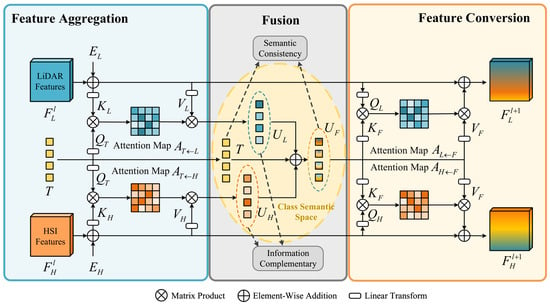
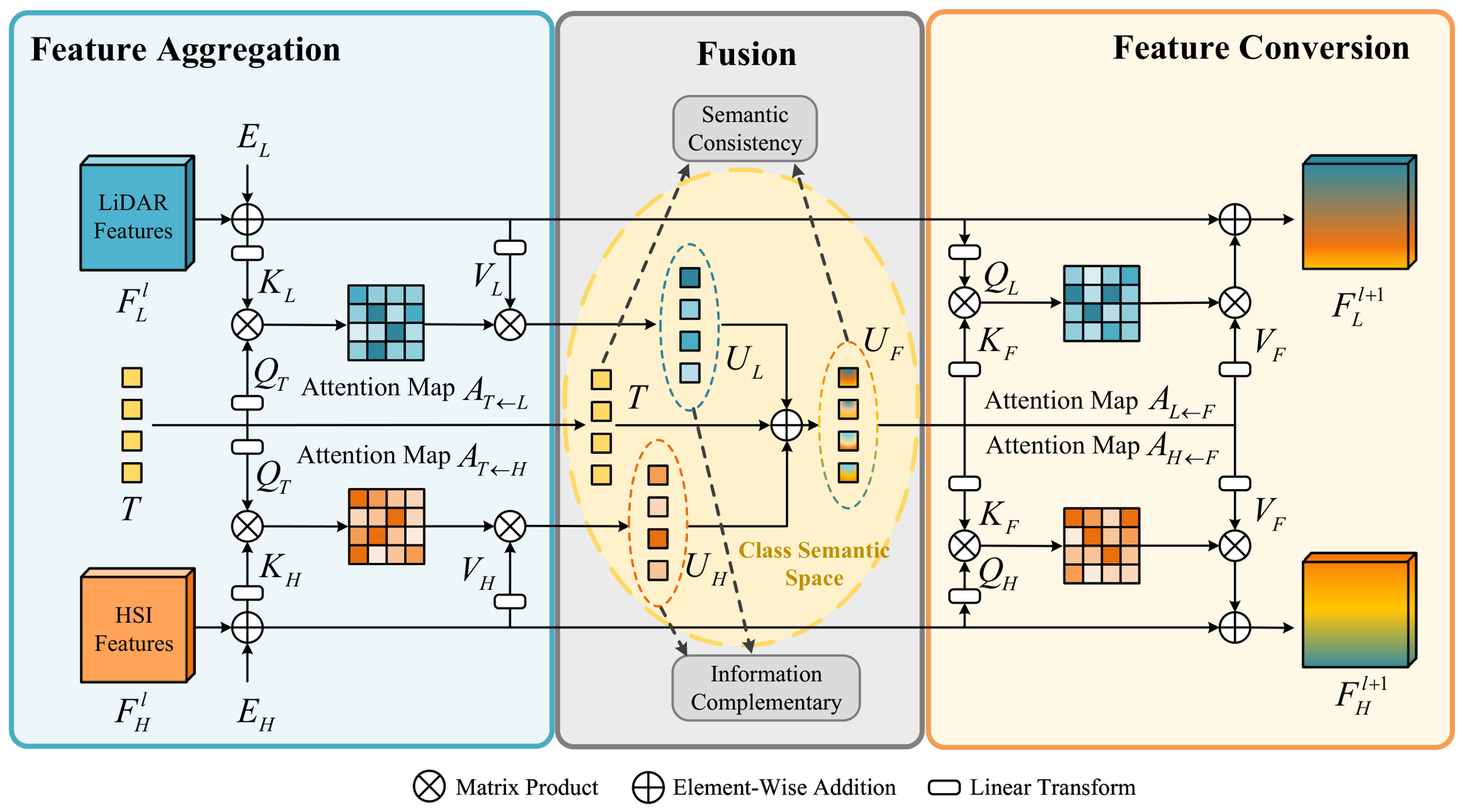
To address the semantic ambiguity and redundancy in existing feature fusion and interaction methods, we introduce a module that achieves semantic-aligned feature aggregation and fusion feature conversion under the guidance of CSP, enabling effective fusion and interaction for improving the precision of HSI and LiDAR classification, the overall framework is illustrated in Figure 2. It is completed by the following stages:
Figure 2.
Graphical illustration of the proposed FFIM. The framework is built upon a cross-attention mechanism. The CSP acts as the query to aggregate features for fusion. The fused output is then used as the key and value to enable feature interaction. Semantic consistency aligns fused features with the CSP, and the information complementarity constraint discourages redundant responses between modalities.
2.3.1. Class Semantic Prototype
To achieve efficient fusion and interaction of cross-modal features, the guidance of high-level semantics is imperative. We therefore introduce a set of learnable CSP as the cornerstone of our fusion framework. We define the CSP as a parameter matrix S denoted as:
where K denotes the number of land-cover classes, and denotes the learnable semantic prototype associated with the k-th class which intended to encapsulate its fundamental semantic essence.
The key to the CSP design lies in its shared parameters with the final classification layer. This critical choice implies that the CSP is not merely passive references but is actively optimized to be the most discriminative center for class separation during training. As a result, they establish a task-oriented semantic space that naturally guides the cross-modal feature fusion and interaction. This mechanism ensures that the entire process, from fusion to classification, is coherently driven by the same semantic objective, thereby operating in a fully task-oriented manner.
2.3.2. Semantic-Aligned Feature Aggregation for Fusion
The introduction of CSP provides a discriminative center for each category. Building upon this, we leverage a cross-attention mechanism where the CSP serves as queries to aggregate semantically relevant features from each modality. This process achieves cross-modal semantic alignment for subsequent fusion. In addition, we also introduce a token to learn global features from both modalities at the same time. It does not represent the features of a certain category, but realizes feature aggregation from modal features which is concatenated with the matrix S:
where the first row of corresponds to the l-th layer of classification token, whereas the remaining K rows correspond to the class semantic prototype.
As the fusion process happens in a symmetrical way for two modalities, we take the l-th FFIM layer as an example. For feature aggregation, we first add the 2D sinusoidal positional encoding to the HSI and LiDAR respectively, and then shape it into , which can be denoted as:
The semantic token matrix , composed of the classification token and the class semantic prototypes, is used to generate the query, while the flattened modality feature , , provides the key and value:
where , , and are learnable linear projection matrices, and d denotes the query–key embedding dimension. Then, the attention map is obtained by applying scaled dot-product attention between the CSP-derived queries and the keys projected from the multimodal tokens:
where each row of , and each represents the normalized relevance between one semantic token and the P spatial tokens of modality m. These attention weights are applied to to selectively aggregate global and class-specific task-relevant information, producing . Because the same semantic tokens query both modalities, and are organized according to a common semantic structure, thereby facilitating their semantic alignment and subsequent element-wise fusion:
where and are aggregated by CSP in this framework which exhibit a degree of semantic alignment. This relationship facilitates the design of constraints that regulate the complementarity among modalities and the effectiveness of the fusion features. Accordingly, we introduce additional loss functions in the subsequent method to impose such constraints.
2.3.3. Fusion Feature Conversion for Interaction
The complementary information can be mined by the cross-modal feature interaction. The fusion features, refined by the CSP, possess enhanced effectiveness and lower redundancy. Here, we leverage a cross-attention mechanism where modal-specific features act as queries to convert the fusion features into modality-specific representations, thereby achieving feature interaction for optimization.
To construct the reverse cross-attention, the flattened modality feature , , is used to generate the query, while the semantically fused feature provides the key and value:
where , , and are learnable linear projection matrices, and d denotes the query–key embedding dimension. Then, the attention map is obtained by applying scaled dot-product attention between the queries projected from the multimodal tokens and the keys projected from the fused feature:
where each row of represents the normalized relevance distribution between one spatial token of modality m and the fused semantic tokens. The first fused token contains global task-relevant information, while the remaining K tokens encode class-specific fused semantics. Therefore, the attention map enables each spatial location to adaptively determine which global or class-specific information should be retrieved from the fused representation.
The retrieved semantic information is subsequently transformed into a modality-compatible representation:
Since is represented as a sequence of spatial tokens, it is reshaped back into the two-dimensional feature layout and added to the original modality feature through a residual connection:
where denotes the modality-specific multilayer perceptron, and restores the P spatial tokens to a feature map. The residual connection preserves the original modality-specific characteristics while incorporating complementary information retrieved from the fused semantic representation. Consequently, the updated features and retain their respective spectral–spatial and elevation characteristics while being refined by task-relevant information from the other modality. These updated representations are then passed to the next FFIM layer, forming a cyclic process of semantic-guided aggregation, fusion, and modality-specific feature refinement.
2.3.4. Cyclic Interaction and Classification
By combining the semantic-guided feature aggregation in Section 2.3.2 with the fusion-to-modality feature conversion in Section 2.3.3, each FFIM layer forms a complete bidirectional interaction cycle. Given the modality-specific features and , together with the classification token , the semantic token matrix first aggregates global and class-specific task-relevant information from the two modalities, producing and . These representations are subsequently combined into the fused semantic representation . The first row of , which corresponds to the global classification token, is used to update the classification token for the next layer:
Meanwhile, the reverse cross-attention mechanism described in Section 2.3.3 converts the fused semantic information back into the HSI and LiDAR feature spaces, yielding the updated modality-specific representations and . Therefore, the complete operation of the l-th FFIM layer can be summarized as
The updated modality features and classification token are then fed into the next FFIM layer. Repeating this process enables the modality-specific representations to progressively absorb complementary information, while the classification token continuously accumulates global task-relevant semantics. Since the same class semantic prototype matrix S is shared across all interaction layers, the aggregation, fusion, and feature-conversion processes remain consistently guided by a common class-semantic space. After stacking FFIM layers, the overall interaction process is expressed as
where denotes the total number of FFIM layers, and represents the sequential composition of FFIM layers rather than an algebraic exponentiation.
The final classification token summarizes the task-relevant information progressively aggregated from both HSI and LiDAR throughout the cyclic interaction process. To maintain consistency between semantic guidance and final prediction, the class semantic prototype matrix S is also used as the weight matrix of the final classifier:
The classification logits are then computed as
and the corresponding class probabilities are obtained by
Because each semantic prototype simultaneously serves as the semantic reference for the k-th class and the corresponding classifier weight, it is directly optimized by the classification objective. Consequently, the same class-discriminative semantics consistently guide feature aggregation, cross-modal fusion, modality-specific refinement, and final prediction, establishing a closed-loop task-oriented interaction mechanism.
2.4. Objective Function
In the proposed method, the whole process is constrained by the interactive task and supervised joint classification task with label information. Therefore, we devise a overall loss function comprising three components: information complementarity, semantic consistency and classification loss. For clarity, the batch dimension, which was omitted in the preceding formulations, is explicitly restored here. Given a mini-batch containing B samples, let , , and denote the HSI-specific aggregation representation, LiDAR-specific aggregation representation, and their fused semantic representation produced by the l-th FFIM layer, respectively, where . For the l-th layer and n-th sample, , , and denote the HSI, LiDAR, and fused representations associated with the k-th semantic prototype, respectively, while denotes the corresponding prototype in S. These variables are used in the following loss formulations.
2.4.1. Information Complementarity
We introduce a minimum similarity loss here to constrain features and discourage excessive similarity between the and , that associated with the same semantic, thereby reducing redundant overlap and preserving modality-specific information:
where represent the HSI- and LiDAR-specific aggregation features associated with the k-th class semantic prototype for the n-th sample in the l-th FFIM layer. The notation denotes the Euclidean norm, and is a small positive constant introduced for numerical stability. The absolute cosine similarity penalizes both positive and negative linear correlations between the corresponding modality-specific representations.
2.4.2. Semantic Consistency
We introduce a maximum similarity loss here to align the fused class-specific representations with the corresponding class semantic prototype, thereby improving the task relevance and semantic consistency of the fused representation:
where denotes the fused semantic representation associated with the k-th class prototype for the n-th sample in the l-th FFIM layer, and is the k-th class semantic prototype in S. The cosine similarity measures the directional consistency between the prototype-guided fused representation and its corresponding semantic reference.
2.4.3. Classification Loss
To directly supervise the final land-cover prediction, we adopt the cross-entropy loss, formulated as follows:
where is the one-hot ground-truth indicator, which equals 1 when the n-th sample belongs to the k-th class and 0 otherwise. denotes the predicted probability that the n-th sample belongs to class k, obtained by applying the Softmax function to the classification logits . The cross-entropy loss directly optimizes the final classification prediction and simultaneously updates both the final classification token and the shared class semantic prototype matrix S. Therefore, it not only improves classification accuracy but also provides class-discriminative supervision for the semantic references used throughout the preceding feature aggregation and interaction processes.
2.4.4. Overall Loss
Considering the balanced relationship between the classification objective and the auxiliary complementarity and semantic consistency constraints, the overall loss function can be written as
where is the weighting coefficient.
3. Experimental Setup
3.1. Dataset Description
3.1.1. Houston2013 Dataset
The Houston2013 dataset [42], featured in the ‘IEEE GRSS Data Fusion Contest 2013’, was captured by the National Airborne Centre using the ITRES CASI-1500 sensor over the University of Houston campus and neighboring TX, USA areas. This dataset spans 349 × 1905 spatial dimensions with a 2.5 m resolution. It comprises 144 spectral bands, ranging from 0.38 to 1.05 μm, within the HSI, while LiDAR data consist of a single band. The ground-truth annotations contain 15 land-cover classes and 15,029 labeled samples, including 2832 training samples and 12,197 test samples. Detailed category and sample information are presented in Table 1.
Table 1.
Number of training and test samples in Houston2013, Trento, and MUUFL datasets.
3.1.2. Trento Dataset
The Trento dataset, captured using AISA Eagle sensors, depicts a rural area in Trento, Italy [43]. It spans 166 × 600 spatial dimensions with a 1.0 m spatial resolution and a spectral resolution of 9.2 nm. The HSI comprises 63 bands covering the spectral range of 0.42 to 0.99 μm, while the LiDAR data consist of a single band. Ground-truth annotations include six classes, totaling 30,214 samples, divided into 819 training and 29,395 test samples. Detailed category and sample information can be found in Table 1.
3.1.3. MUUFL Dataset
The MUUFL Gulfport dataset [44,45], collected at 3500 ft, covers the University of Southern Mississippi Gulf Park campus in Long Beach, Mississippi, from November 2010. The dataset was clipped to a spatial size of 325 × 220 with a 1.0 m spatial resolution. The HSI consists of 72 bands, ranging from 0.38 to 1.05 μm. After removing eight noisy bands from the beginning and end of the spectrum, 64 bands are retained. The LiDAR data include two bands. Groundtruth annotation covers 11 classes with a total of 53,687 samples. More detailed category and sample information is outlined in Table 1.
The three datasets follow different sampling protocols because they were released and evaluated under different benchmark conventions. For Houston2013, we use the fixed partition provided for the IEEE GRSS Data Fusion Contest, containing 2832 training samples and 12,197 test samples. For Trento, we adopt the widely used fixed partition consisting of 819 training samples and 29,395 test samples. Retaining these fixed partitions enables direct comparison with previous methods evaluated under the same protocols. In contrast, an equivalent fixed land-cover classification partition is not commonly provided for the MUUFL dataset. Following the balanced sampling protocol adopted in related HSI–LiDAR classification studies, we randomly select 100 labeled samples from each class for training and use all remaining labeled samples for testing. Because the datasets differ in class composition, scene complexity, sample distribution, and training protocol, their absolute accuracies should not be directly compared across datasets. Instead, experimental fairness is evaluated within each dataset by applying an identical sampling protocol to all compared methods.
3.2. Implementation Details
The experiment used to verify the feasibility of this method was performed on the pytorch framework, utilizing an Ubuntu operating system equipped with an Intel Core i5-12400f central processing unit, an NVIDIA GeForce RTX 4090 graphics processing unit, and 32 GB of random access memory. The experiments were implemented using PyTorch 1.13.1 with CUDA 12.2. General training hyperparameters, including the learning rate, batch size, and number of attention heads, were evaluated using multiple candidate settings in repeated preliminary experiments. As these parameters were general optimization settings rather than method-specific architectural factors, we reported only the final configurations adopted in all experiments. Specifically, we used Adam as the optimizer with an initial learning rate of 0.0002 and learning rate decay factor of 0.9, the batch size was 64, and the multi-head attention mechanism employed eight attention heads. The number of training rounds was set to 400. In order to objectively reflect the classification performance, we used the overall accuracy (OA), average accuracy (AA) and coefficient as evaluation criteria.
4. Experimental Results
This section presents the quantitative and qualitative comparisons with competing methods, followed by ablation studies evaluating the effectiveness of the proposed components.
4.1. Comparison Experiments
To evaluate the advancement and effectiveness of CSPGFNet, we compared it with several state-of-the-art HSI and LiDAR fusion classification models, including CCRNet [24], the multi-attention hierarchical fusion network (MAHiDFNet) [34], multimodal fusion transformer (MFT) [37], global–local transformer network (GLTNet) [29], the dynamic-scale hierarchical fusion network (DSHFNet) [46], coupled adversarial learning (CALC) [28], coarse-to-fine high-order network (CHNet) [41] and multiscale cross-domain fusion network (MCFNet) [40]. To ensure fair comparisons, all models were implemented using the optimal parameters reported in the corresponding references. The same training and testing samples were used across all methods, and results are reported as mean values with standard deviations, which helps mitigate the impact of random experimental variations and enhances the comparability of the methods.
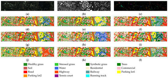
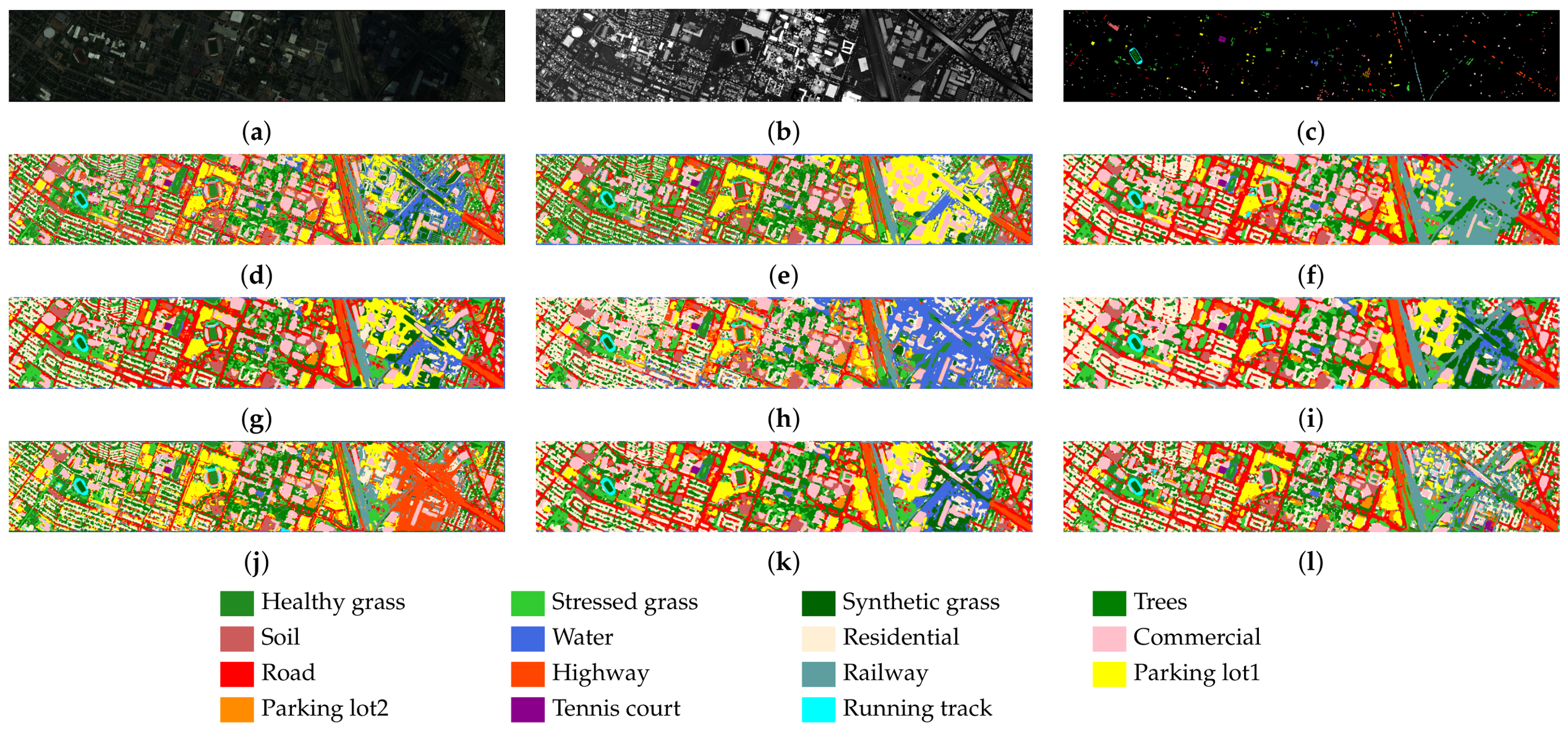
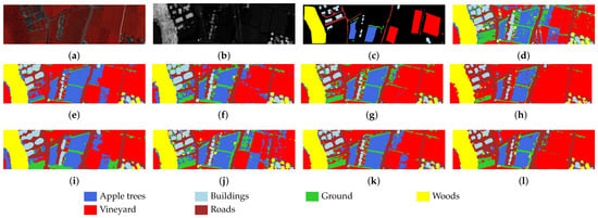
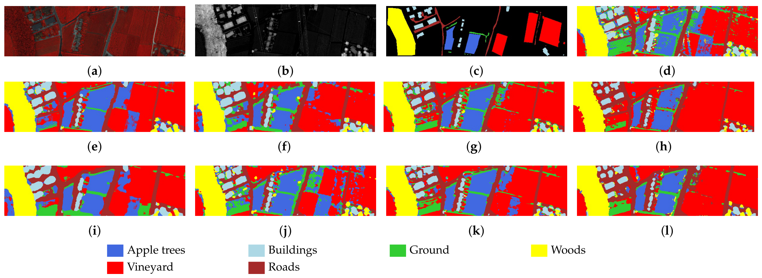
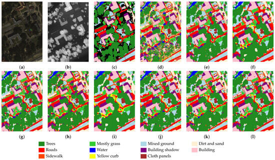
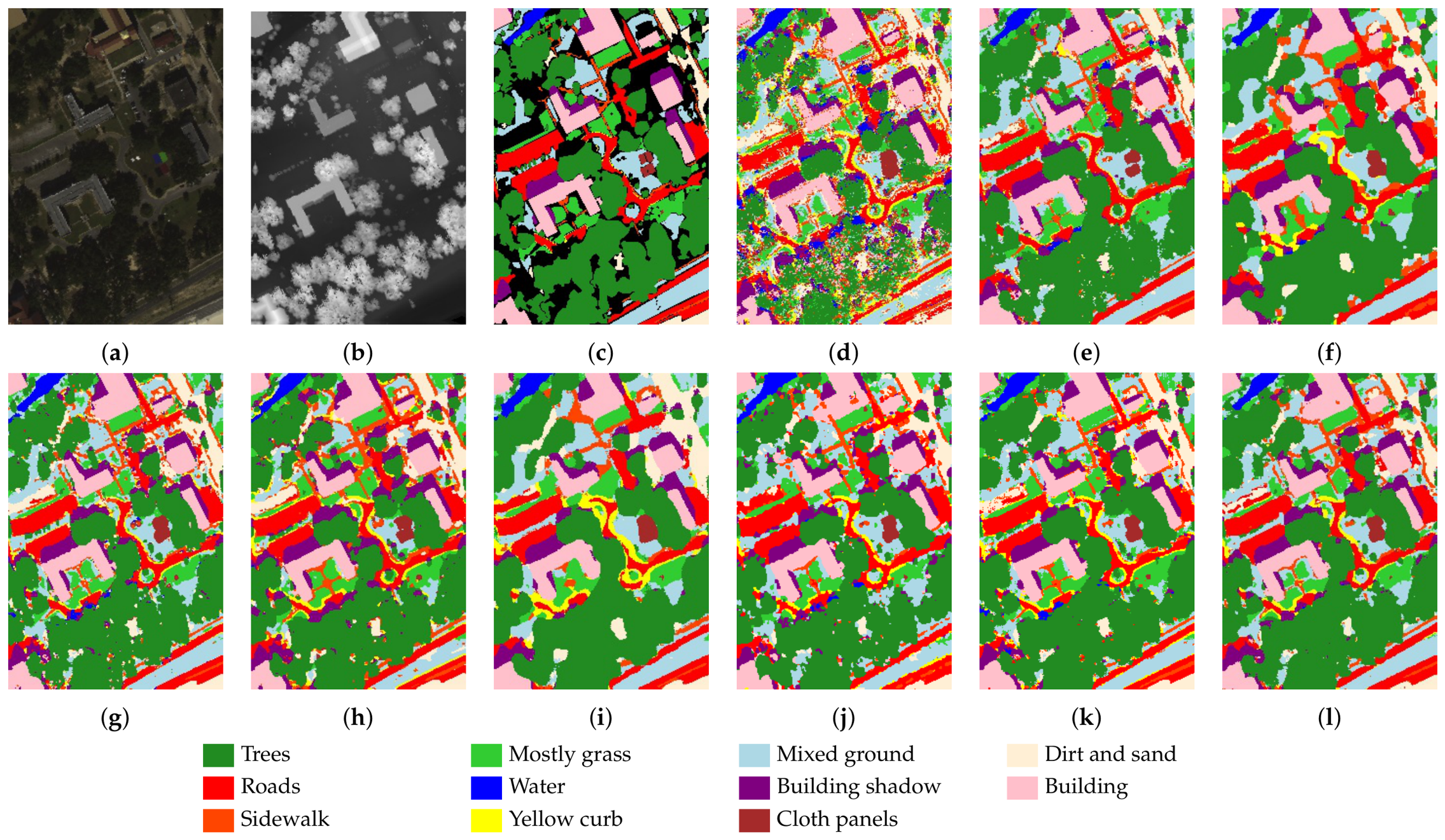
The experimental results include both quantitative analysis and visualizations. The quantitative results are presented in Table 2, Table 3 and Table 4, where the highest accuracy in each row is highlighted in bold. The visual results are shown in Figure 3, Figure 4 and Figure 5, which display pseudocolor images of HSI, LiDAR image, ground truth map, and classification maps generated by different methods. The figures also include color legends indicating the class labels.
Table 2.
Classification results in terms of OA (%), AA (%), and for different methods on the Houston2013 dataset. The best result in each row is shown in bold.
Table 3.
Classification results in terms of OA (%), AA (%), and for different methods on the Trento dataset. The best result in each row is shown in bold.
Table 4.
Classification results in terms of OA (%), AA (%), and for different methods on the MUUFL dataset. The best result in each row is shown in bold.
Figure 3.
Visualization results of different methods on Houston2013 dataset and corresponding semantic class color legend. (a) Pseudocolor image for HSI. (b) LiDAR image. (c) Ground-truth map. (d) CCRNet. (e) MAHiDFNet. (f) MFT. (g) GLTNet. (h) DSHFNet. (i) CALC. (j) CHNet. (k) MCFNet. (l) Ours.
Figure 4.
Visualization results of different methods on Trento dataset and corresponding semantic class color legend. (a) Pseudocolor image for HSI. (b) LiDAR image. (c) Ground-truth map. (d) CCRNet. (e) MAHiDFNet. (f) MFT. (g) GLTNet. (h) DSHFNet. (i) CALC. (j) CHNet. (k) MCFNet. (l) Ours.
Figure 5.
Visualization results of different methods on MUUFL dataset and corresponding semantic class color legend. (a) Pseudocolor image for HSI. (b) LiDAR image. (c) Ground-truth map. (d) CCRNet. (e) MAHiDFNet. (f) MFT. (g) GLTNet. (h) DSHFNet. (i) CALC. (j) CHNet. (k) MCFNet. (l) Ours.
4.1.1. Houston2013 Dataset Results
As shown in Table 2, CSPGFNet achieves an of 93.32%, of 94.02% and of 0.9275, which are 0.45%, 0.68% and 0.0049 higher than the second-best method. CSPGFNet improves the classification accuracy of Class 10 to a certain extent, while also enhancing the overall classification performance across all categories. Notably, 13 out of the 15 classes achieved an accuracy of over 90%. This improvement can be attributed to our CSPGFNet method, which leverages the classification linear layer to aggregate features. It effectively filters out redundant information while integrating class-specific cues, enabling the fused features at each pixel to be more representative of their respective classes and more discriminative. Moreover, from the visualizations in Figure 3, CSPGFNet does not exhibit significant feature blurring or block confusion in regions affected by cloud and fog occlusion. Instead, it preserves the original spatial structure to the greatest extent possible.
4.1.2. Trento Dataset Results
As shown in Table 3, CSPGFNet achieves an of 99.39%, of 98.25% and of 0.9918, which are 0.14%, 0.08% and 0.0018 higher than the second-best approach. Our method achieves competitive class-wise performance, with six classes achieving an accuracy of over 94%. From the visual results shown in Figure 4, CSPGFNet exhibits smooth and coherent classification maps without excessive isolated misclassified pixels. In particular, the road class shows a continuous and well-defined distribution, while the building class maintains complete spatial integrity without category leakage or salt-and-pepper artifacts. Moreover, in the lower-left region containing numerous small and complex objects, the proposed method produces clear and well-separated clusters for each category, effectively reducing ambiguity and preserving fine structural details.
4.1.3. MUUFL Dataset Results
As shown in Table 4, CSPGFNet achieves an of 92.01%, of 92.22% and of 0.8941, which are 1.26%, 0.68% and 0.0156 higher than the second-best approach. From the visual results in Figure 5, it can be observed that the classification map generated by CSPGFNet exhibits spatial contours that closely resemble the original image. In particular, the building and road classes show no signs of category leakage, which demonstrates a strong ability to preserve the authentic spatial structure of the building class. At the same time, in complex small-scale regions such as crossroads in the central area, the model accurately distinguishes each category without confusion or boundary artifacts, thus maintaining the original spatial organization and geometric integrity of the scene in the classification results. It can be attributed to the de-redundancy capability of the CSPGFNet, which enhances the distinction between different classes by effectively removing redundant information.
In summary, the experimental results across all three datasets consistently demonstrate the superiority of our method.
4.2. Ablation Studies
To validate the effectiveness of the proposed modules—including the feature extraction module, the feature fusion and interaction module, and the objective function—we conduct a series of ablation studies. The results further confirm the contribution and necessity of each component to the overall performance improvement. Meanwhile, we conducted a model complexity analysis under the following settings: For all three datasets, the input patch sizes were selected according to the optimal configurations identified in the parameter sensitivity analysis, while the input channel dimensions and the number of output classes were determined according to the corresponding dataset configurations. Specifically, the HSI/LiDAR channel numbers and the numbers of output classes were and 15 for the Houston2013 dataset, and 6 for the Trento dataset, and and 11 for the MUUFL dataset, respectively. The results are presented in the Table 5.
Table 5.
Ablation results in terms of OA (%), AA (%), and on the Houston2013, Trento, and MUUFL datasets.
4.2.1. Feature Extraction Module (FEM)
Due to the inherent dimensional differences between hyperspectral and LiDAR data, there exists a significant information gap between the two modalities. A single-scale feature extraction strategy may exacerbate the feature diversity imbalance introduced by these raw data discrepancies. To verify the effectiveness of the multi-scale convolutional design in the LiDAR feature extraction branch, we replace the proposed module with a conventional 2D convolution-based feature extractor. Specifically, the comparison module consists of two sequential convolutional layers, which maintains a comparable receptive field and computational complexity with the original feature extraction module. Different from the proposed multi-scale convolution, the standard convolution adopts a fixed kernel size and lacks the ability to capture structural information at multiple spatial scales. Compared to the single-scale baseline, the concatenation of multi-scale features provides higher diversity and more comprehensive semantic information. As shown in the first rows of Table 5, enhancing the balance of feature diversity within the attention mechanism leads to notable improvements in classification accuracy.
4.2.2. Feature Fusion and Interaction Module (FFIM)
The FFIM module is a key innovation of our proposed framework. To evaluate the effectiveness of feature aggregation for semantically aligned fusion and cyclic interaction for refinement based on cross-attention, we removed the interaction between modalities in the experiment. However, we retained the basic framework, including CSP and the loss functions, to conduct an ablation study to verify the role of inter-modal information interaction. As shown in second row of Table 5, the interaction between modalities enables the complementarity of information, leading to improved classification accuracy across different datasets.
4.2.3. Class Semantic Prototype (CSP)
To verify the effectiveness of using shared weights between the classification linear layer and the CSP for semantic guidance, we replaced it with a learnable task-agnostic matrix in the FFIM module. The results demonstrate that sharing classifier weights as semantic prototype establishes a task-aware semantic reference, thereby ensuring that feature aggregation and interaction are consistently guided toward task-relevant objectives. This semantic-aware design enhances fusion effectiveness, with particularly pronounced improvements in challenging scenes such as those in the Houston2013 dataset.
4.2.4. Objective Function (OF)
The design of the objective function naturally facilitates the incorporation of loss-based constraints. To evaluate their impact, we conducted ablation studies by removing the information complementary and semantic consistency losses. The results show that introducing the loss significantly reduces redundancy in the aggregated cross-modal features and enhances their complementarity. Moreover, the fusion features become more discriminative and semantically consistent, leading to a notable improvement in classification accuracy.
4.2.5. Effectiveness of Multimodal Fusion
To ensure experimental fairness, we uniformly controlled the parameter scale of each sub-model. The experimental results, as shown in rows 5 and 6 of Table 5, indicate that regardless of which modality is removed, system performance declines to varying degrees, demonstrating the complementary nature of multimodal information. As can be seen from the experimental results on the three datasets, the more complex the terrain, the more difficult it is for the patch-based method to classify LiDAR data, while hyperspectral data still plays a dominant role in classification accuracy.
5. Discussion
5.1. Parameter Sensitivity Analysis
5.1.1. Input Patch Size
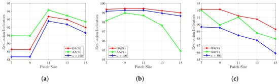
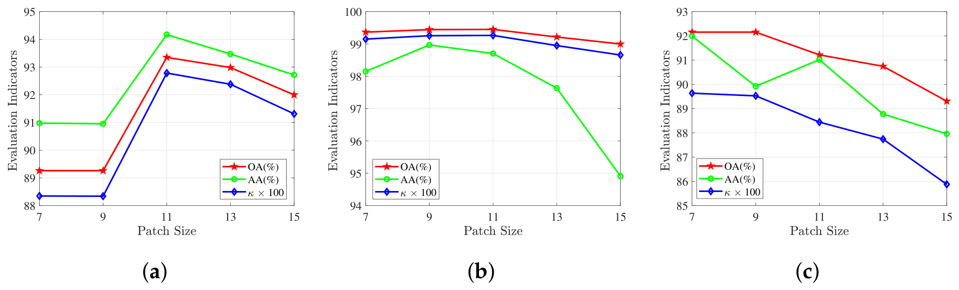
The decision on the appropriate patch size is vital as using a large patch size introduces unnecessary information while utilizing a small patch size misses details. Figure 6 illustrates the impact of input patch size range from 7 to 15. The results show that the optimal patch size for the Houston and Trento datasets is 11, while the optimal patch size for the MUUFL dataset is 7. This difference is mainly attributed to the variations in spatial scale across different datasets, and partially due to the different ways in which each model processes the data.
Figure 6.
Effect of patch size for CSPGFNet. (a) Houston2013. (b) Trento. (c) MUUFL.
The optimal patch size varies across different datasets due to their distinct spatial structures and land-cover distributions. When the input patch size is too small, insufficient spatial context limits the ability of CSP-guided cross-modal interaction to exploit complementary spectral and structural information, resulting in less discriminative semantic representations. As the patch size increases, richer neighborhood information enables more effective semantic aggregation and improves classification performance. However, excessively large patches may introduce irrelevant surrounding regions and background interference, weakening the discriminability of the target pixel. Specifically, Houston2013 and Trento achieve the best performance with an patch size because their heterogeneous scenes and complex spatial layouts require larger contextual information to distinguish similar categories. In contrast, MUUFL achieves the optimal result with a smaller patch size, indicating that its local spatial patterns already provide sufficient discriminative information, while larger patches may introduce unnecessary spatial redundancy. Therefore, the selected patch sizes reflect a trade-off between exploiting useful contextual information and reducing irrelevant spatial interference.
5.1.2. Network Depth
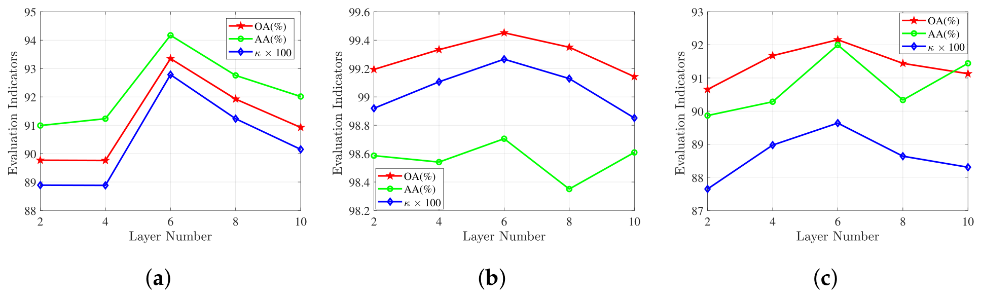
For Transformer-based networks with limited training data, increasing the number of FFIM layers enables more rounds of semantic-guided interaction between HSI and LiDAR, allowing complementary information to be progressively aggregated and refined. Consequently, the classification performance improves in the early stage. However, when the network becomes deeper, repeated feature interaction gradually introduces redundant semantic information and increases optimization difficulty. Meanwhile, excessive interaction may reduce the diversity of modality-specific representations, leading to marginal performance degradation. Therefore, an appropriate network depth achieves the best balance between semantic interaction and feature preservation. As illustrated in Figure 7, the optimal performance is achieved with six layers across all three datasets.
Figure 7.
Effect of network depth for CSPGFNet. (a) Houston2013. (b) Trento. (c) MUUFL.
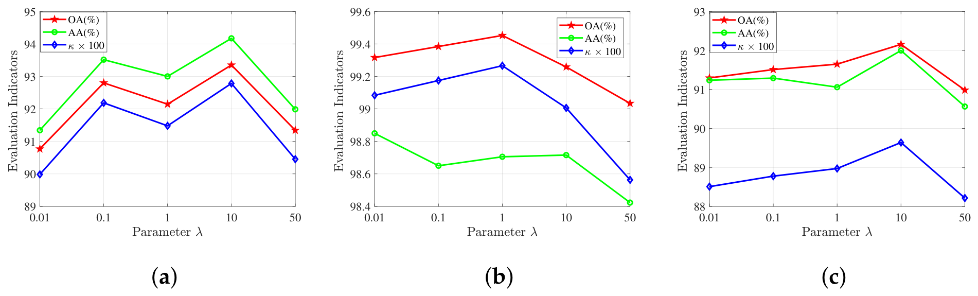
5.1.3. Loss Coefficient
In Section 2, it is mentioned that parameter represents the weighting coefficient of the constraint loss in the total loss. The magnitude of this parameter determines the model’s emphasis on the constraint loss during backpropagation and governs the degree to which the constraints are enforced on the Section 2.4 throughout the convergence process. Figure 8 illustrates the impact of parameter range from 0.01 to 50. When is too small, the complementarity and semantic consistency losses cannot provide sufficient guidance for feature fusion, making the optimization dominated by the classification objective. Conversely, an excessively large overemphasizes the auxiliary constraints, weakening the contribution of the classification supervision and causing a slight performance decrease. Therefore, an intermediate value achieves the best trade-off between classification optimization and semantic regularization. The results show that the optimal parameter for the Houston and MUUFL dataset is 10, while the optimal parameter for the Trento dataset is 1.
Figure 8.
Effect of parameter on CSPGFNet. (a) Houston2013. (b) Trento. (c) MUUFL.
5.2. Complexity Analysis
To evaluate the computational efficiency of the proposed method, we compare the number of parameters, FLOPs, and the training/testing time with several representative HSI-LiDAR classification methods on the Houston2013, Trento, and MUUFL datasets. The results are summarized in Table 6.
Table 6.
Comparison of the number of parameters, FLOPs, and training/testing time.
Overall, the proposed method achieves an excellent balance between classification performance and computational efficiency. Specifically, our method contains 252.00 K, 203.04 K, and 189.34 K parameters on the Houston2013, Trento, and MUUFL datasets, respectively, which are substantially smaller than heavy CNN-based methods such as CHNet (approximately 20.8 M parameters) and MAHiDFNet, while remaining comparable to lightweight transformer-based methods including CCRNet, MFT, GLTNet, and MCFNet.
In terms of computational complexity, the proposed method requires 83.52 M, 58.28 M, and 55.16 M FLOPs on the three datasets, respectively. Although the FLOPs are slightly higher than those of some lightweight methods (e.g., CCRNet and MFT), they remain significantly lower than those of GLTNet, DSHFNet, and CHNet, demonstrating that the proposed semantic-guided feature interaction introduces only a moderate computational overhead.
Regarding computational efficiency, the proposed method achieves competitive runtime performance. It requires only 551.12 s, 146.19 s, and 246.52 s for training on the Houston2013, Trento, and MUUFL datasets, respectively, which is faster than most competing methods. Similarly, the corresponding testing times are 1.47 s, 3.26 s, and 5.71 s, remaining substantially lower than those of computationally intensive methods such as GLTNet, DSHFNet, CHNet, and MCFNet. These results indicate that the proposed CSP-guided feature fusion strategy effectively enhances semantic representation without introducing excessive computational cost, achieving a favorable trade-off between model complexity and efficiency.
5.3. Feature Representation Analysis
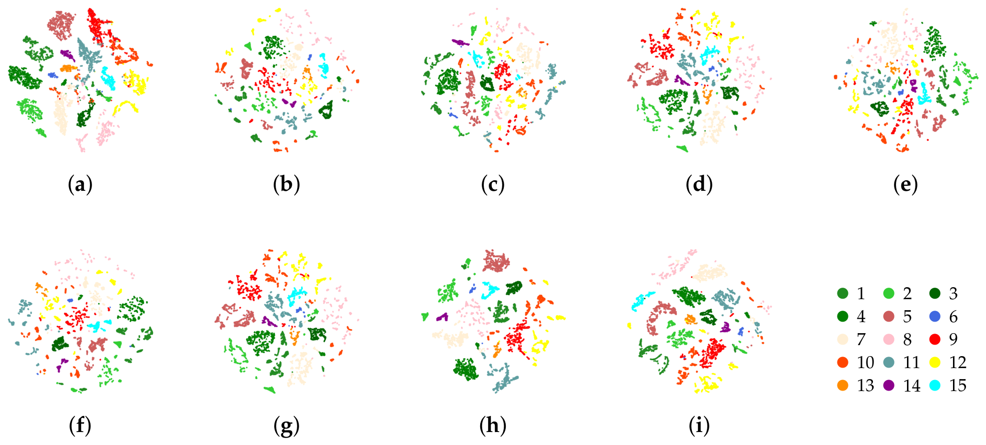
To further investigate the discriminative capability of the learned feature representations, t-SNE visualization is employed to project the high-dimensional fused features into a two-dimensional space. In this experiment, only the Houston2013 dataset is selected for visualization. The main reason is that Houston2013 contains 15 land-cover categories with a relatively balanced distribution of test samples among different classes, which provides a more comprehensive evaluation of feature separability. In contrast, the Trento dataset contains fewer categories, making it less sufficient for observing complex inter-class relationships, while the MUUFL dataset exhibits a significant imbalance in the number of samples among different classes, which may affect the visual interpretation of feature distributions. Therefore, Houston2013 provides a more representative and intuitive scenario for analyzing the discriminative characteristics of learned features.
As shown in Figure 9, compared with the competing methods, the proposed CSPGFNet produces a more compact and well-separated feature distribution. Specifically, the samples belonging to the same category are concentrated into tighter clusters, indicating improved intra-class compactness. Meanwhile, different land-cover categories exhibit clearer boundaries with fewer overlapping regions, demonstrating enhanced inter-class separability. This advantage can be attributed to the class semantic prototype guided fusion strategy. By sharing parameters with the final classifier, the CSPs provide task-oriented semantic references during cross-modal feature aggregation, enabling the network to selectively capture category-relevant spectral, spatial, and elevation information rather than indiscriminately combining heterogeneous features. Furthermore, the semantic consistency constraint encourages the fused representations to remain aligned with their corresponding class prototypes, which further enhances the aggregation of intra-class features and increases the discriminability between different classes.
Figure 9.
Visualization results via t-SNE of different methods on Houston2013 dataset and corresponding class color legend. (a) CCRNet. (b) MAHiDFNet. (c) MFT. (d) GLTNet. (e) DSHFNet. (f) CALC. (g) CHNet. (h) MCFNet. (i) CSPGFNet. Different land-cover classes are plotted in different colors.
Overall, the t-SNE visualization indicates that the proposed CSPGFNet can effectively learn a more discriminative semantic feature space. The improved feature organization demonstrates that prototype-guided semantic alignment not only facilitates complementary information integration between HSI and LiDAR modalities but also reduces redundant and ambiguous responses caused by heterogeneous modal characteristics. Consequently, the learned representations become more suitable for accurate land-cover classification.
5.4. Limitations and Future Perspectives
Although the proposed CSPGFNet demonstrates competitive performance on three benchmark HSI–LiDAR datasets, several limitations remain. First, the proposed class semantic prototypes are learned under a supervised closed-set setting, and their applicability to few-shot or open-set scenarios deserves further investigation. Second, the current framework follows the commonly adopted patch-based classification paradigm and assumes accurate spatial alignment between HSI and LiDAR data. Its robustness to severe cross-modal misregistration has not been explicitly considered. Finally, the proposed method has been evaluated on benchmark datasets with predefined protocols, while its cross-region and cross-sensor generalization capability requires further validation. In future work, we will explore adaptive prototype learning, learnable cross-modal alignment mechanisms, and domain adaptation techniques to further improve the flexibility and practical applicability of the proposed framework.
6. Conclusions
This paper introduces a CSPGFNet for multimodal fusion, aiming to reduce semantic discrepancy and redundancy between modalities while enhancing the complementarity and effectiveness of cross-modal feature integration to improve classification performance. The core of our approach lies in leveraging a learnable class semantic prototype as a shared semantic bridge, which drives a cyclic cross-attention mechanism to achieve task-aligned feature aggregation for fusion and closed-loop information interaction for inter-modal refinement. Moreover, additional constraints are introduced to further enhance the complementarity and effectiveness of the fused features. Extensive experiments demonstrate the superiority of the proposed model.
Author Contributions
Conceptualization, Z.D.; methodology, X.X. and Z.D.; software, X.X. and Y.S.; validation, X.X. and Y.S.; resources, H.W.; data curation, X.X., D.S. and Y.S.; writing—original draft preparation, X.X.; writing—review and editing, D.S. and Z.D.; visualization, X.X. and Y.S.; supervision, D.S. and H.W.; project administration, H.W.; funding acquisition, Z.D. All authors have read and agreed to the published version of the manuscript.
Funding
This research was funded by the National Key R&D Program of China, grant number 2025YFE0209600, Liaoning Young Elite Scientists Sponsorship Program, and Dalian Young Star of Science and Technology Project.
Data Availability Statement
The publicly available datasets used in this study are as follows: the Houston2013 dataset is provided by the Hyperspectral Image Analysis group and the NSF Funded Center for Airborne Laser Mapping (NCALM) at the University of Houston, originally used for the 2013 IEEE GRSS Data Fusion Contest, available at: https://hyperspectral.ee.uh.edu/?page_id=1075 (accessed on 26 November 2023); the Trento dataset is provided by Professor Lorenzo Bruzzone of the University of Trento, available at: https://github.com/tyust-dayu/Trento (accessed on 21 January 2024); the MUUFL Gulfport dataset is provided by the GatorSense group at the University of Florida, available at: https://github.com/GatorSense/MUUFLGulfport (accessed on 26 November 2023). Further inquiries can be directed to the corresponding author.
Acknowledgments
The authors are grateful to the Hyperspectral Image Analysis group and the NSF Funded Center for Airborne Laser Mapping (NCALM) at the University of Houston for providing the Houston2013 dataset used in this study; to Professor Lorenzo Bruzzone of the University of Trento for providing the Trento dataset; and to the GatorSense group at the University of Florida for providing the MUUFL Gulfport dataset.
Conflicts of Interest
The authors declare no conflicts of interest.
References
- Zhao, F.; Zhang, C.; Geng, B. Deep multimodal data fusion. ACM Comput. Surv. 2024, 56, 216. [Google Scholar] [CrossRef] [Scilit]
- Li, J.; Hong, D.; Gao, L.; Yao, J.; Zheng, K.; Zhang, B.; Chanussot, J. Deep learning in multimodal remote sensing data fusion: A comprehensive review. Int. J. Appl. Earth Obs. Geoinf. 2022, 112, 102926. [Google Scholar] [CrossRef] [Scilit]
- Yu, H.; Ling, Z.; Zheng, K.; Gao, L.; Li, J.; Chanussot, J. Unsupervised hyperspectral and multispectral image fusion with deep spectral-spatial collaborative constraint. IEEE Trans. Geosci. Remote Sens. 2024, 62, 5534114. [Google Scholar] [CrossRef] [Scilit]
- Jia, J.; Yu, H.; Wang, C.; Zheng, K.; Li, J.; Hu, J. Spectral-Spatial Collaborative Pretraining Framework with Multi-Constraint Cooperation for Hyperspectral-Multispectral Image Fusion. IEEE J. Sel. Top. Appl. Earth Obs. Remote Sens. 2025, 18, 11610–11622. [Google Scholar] [CrossRef] [Scilit]
- Li, J.; Ma, Y.; Song, R.; Xi, B.; Hong, D.; Du, Q. A triplet semisupervised deep network for fusion classification of hyperspectral and LiDAR data. IEEE Trans. Geosci. Remote Sens. 2022, 60, 5540513. [Google Scholar] [CrossRef] [Scilit]
- Guo, F.; Meng, Q.; Li, Z.; Ren, G.; Wang, L.; Zhang, J.; Xin, R.; Hu, Y. Multisource feature embedding and interaction fusion network for coastal wetland classification with hyperspectral and LiDAR data. IEEE Trans. Geosci. Remote Sens. 2024, 62, 5509516. [Google Scholar] [CrossRef] [Scilit]
- Shen, D.; Ma, X.; Kong, W.; Liu, J.; Wang, J.; Wang, H. Hyperspectral target detection based on interpretable representation network. IEEE Trans. Geosci. Remote Sens. 2023, 61, 5519416. [Google Scholar] [CrossRef] [Scilit]
- Lu, B.; Dao, P.D.; Liu, J.; He, Y.; Shang, J. Recent advances of hyperspectral imaging technology and applications in agriculture. Remote Sens. 2020, 12, 2659. [Google Scholar] [CrossRef] [Scilit]
- Kong, W.; Shen, D.; Li, M.; Ma, X.; Wang, H. Hyperspectral anomaly detection based on tensor approximation with tensor double nuclear norm. IEEE Trans. Geosci. Remote Sens. 2025, 63, 5507414. [Google Scholar] [CrossRef] [Scilit]
- He, Y.; Xi, B.; Li, G.; Zheng, T.; Li, Y.; Xue, C.; Chanussot, J. Multilevel attention dynamic-scale network for HSI and LiDAR data fusion classification. IEEE Trans. Geosci. Remote Sens. 2024, 62, 5529916. [Google Scholar] [CrossRef] [Scilit]
- Huo, L.; Xia, J.; Zhang, L.; Zhang, H.; Xu, M. Center-bridged Interaction Fusion for hyperspectral and LiDAR classification. Neurocomputing 2024, 590, 127757. [Google Scholar] [CrossRef] [Scilit]
- Chanussot, J.; Benediktsson, J.A.; Fauvel, M. Classification of remote sensing images from urban areas using a fuzzy possibilistic model. IEEE Geosci. Remote Sens. Lett. 2006, 3, 40–44. [Google Scholar] [CrossRef] [Scilit]
- Wang, R.; Gamon, J.A.; Cavender-Bares, J.; Townsend, P.A.; Zygielbaum, A.I. The spatial sensitivity of the spectral diversity–biodiversity relationship: An experimental test in a prairie grassland. Ecol. Appl. 2018, 28, 541–556. [Google Scholar] [CrossRef] [Scilit] [PubMed]
- Bai, J.; Huang, H.; He, B.; Ma, L.; Gao, S.; Peng, S.; Yang, X.; Hao, Y.; Dong, Y.; Bi, K.; et al. The first large-footprint hyperspectral LiDAR model to attempt to reveal forest chlorophyll distribution heterogeneity from vertically layered spectral perspective utilizing 3D radiative transfer modeling. Int. J. Appl. Earth Obs. Geoinf. 2026, 146, 105060. [Google Scholar] [CrossRef] [Scilit]
- Bai, J.; Zhu, J.; He, B.; Qian, B.; Wang, L.; Niu, Z.; Li, S. Edge Effect Issue on Hyperspectral LiDAR Point Cloud Data: Generation Principle and Framework of Detection and Filtering. IEEE Trans. Geosci. Remote Sens. 2026, 64, 5702610. [Google Scholar] [CrossRef] [Scilit]
- Liu, C.; Qian, J.; Fang, F. ISGM-Fus: Internal structure-guided model for multispectral and hyperspectral image fusion. Neurocomputing 2025, 650, 130777. [Google Scholar] [CrossRef] [Scilit]
- Song, T.; Zeng, Z.; Gao, C.; Chen, H.; Li, J. Joint classification of hyperspectral and lidar data using height information guided hierarchical fusion-and-separation network. IEEE Trans. Geosci. Remote Sens. 2024, 62, 5505315. [Google Scholar] [CrossRef] [Scilit]
- Hong, D.; Han, Z.; Yao, J.; Gao, L.; Zhang, B.; Plaza, A.; Chanussot, J. SpectralFormer: Rethinking hyperspectral image classification with transformers. IEEE Trans. Geosci. Remote Sens. 2021, 60, 5518615. [Google Scholar] [CrossRef] [Scilit]
- Song, W.; Gao, Z.; Zhang, Y. Discriminative feature extraction and fusion for classification of hyperspectral and LiDAR data. In Proceedings of the IGARSS 2022—2022 IEEE International Geoscience and Remote Sensing Symposium; IEEE: New York, NY, USA, 2022; pp. 2271–2274. [Google Scholar]
- Ghamisi, P.; Rasti, B.; Yokoya, N.; Wang, Q.; Hofle, B.; Bruzzone, L.; Bovolo, F.; Chi, M.; Anders, K.; Gloaguen, R.; et al. Multisource and multitemporal data fusion in remote sensing: A comprehensive review of the state of the art. IEEE Geosci. Remote Sens. Mag. 2019, 7, 6–39. [Google Scholar] [CrossRef] [Scilit]
- Liu, B.; Yu, X.; Zhang, P.; Yu, A.; Fu, Q.; Wei, X. Supervised deep feature extraction for hyperspectral image classification. IEEE Trans. Geosci. Remote Sens. 2017, 56, 1909–1921. [Google Scholar] [CrossRef] [Scilit]
- Chen, Y.; Lin, Z.; Zhao, X.; Wang, G.; Gu, Y. Deep learning-based classification of hyperspectral data. IEEE J. Sel. Top. Appl. Earth Obs. Remote Sens. 2014, 7, 2094–2107. [Google Scholar] [CrossRef] [Scilit]
- Hong, D.; Gao, L.; Yokoya, N.; Yao, J.; Chanussot, J.; Du, Q.; Zhang, B. More diverse means better: Multimodal deep learning meets remote-sensing imagery classification. IEEE Trans. Geosci. Remote Sens. 2020, 59, 4340–4354. [Google Scholar] [CrossRef] [Scilit]
- Wu, X.; Hong, D.; Chanussot, J. Convolutional neural networks for multimodal remote sensing data classification. IEEE Trans. Geosci. Remote Sens. 2021, 60, 5517010. [Google Scholar] [CrossRef] [Scilit]
- Roy, S.K.; Deria, A.; Hong, D.; Ahmad, M.; Plaza, A.; Chanussot, J. Hyperspectral and LiDAR data classification using joint CNNs and morphological feature learning. IEEE Trans. Geosci. Remote Sens. 2022, 60, 5530416. [Google Scholar] [CrossRef] [Scilit]
- Feng, J.; Feng, X.; Chen, J.; Cao, X.; Zhang, X.; Jiao, L.; Yu, T. Generative adversarial networks based on collaborative learning and attention mechanism for hyperspectral image classification. Remote Sens. 2020, 12, 1149. [Google Scholar] [CrossRef] [Scilit]
- Zhou, H.; Luo, F.; Zhuang, H.; Weng, Z.; Gong, X.; Lin, Z. Attention multihop graph and multiscale convolutional fusion network for hyperspectral image classification. IEEE Trans. Geosci. Remote Sens. 2023, 61, 5508614. [Google Scholar] [CrossRef] [Scilit]
- Lu, T.; Ding, K.; Fu, W.; Li, S.; Guo, A. Coupled adversarial learning for fusion classification of hyperspectral and LiDAR data. Inf. Fusion 2023, 93, 118–131. [Google Scholar] [CrossRef] [Scilit]
- Ding, K.; Lu, T.; Fu, W.; Li, S.; Ma, F. Global–local transformer network for HSI and LiDAR data joint classification. IEEE Trans. Geosci. Remote Sens. 2022, 60, 5541213. [Google Scholar] [CrossRef] [Scilit]
- Yang, J.Y.; Li, H.C.; Hu, W.S.; Pan, L.; Du, Q. Adaptive cross-attention-driven spatial–spectral graph convolutional network for hyperspectral image classification. IEEE Geosci. Remote Sens. Lett. 2021, 19, 6004705. [Google Scholar] [CrossRef] [Scilit]
- Yang, J.X.; Zhou, J.; Wang, J.; Tian, H.; Liew, A.W.C. LiDAR-guided cross-attention fusion for hyperspectral band selection and image classification. IEEE Trans. Geosci. Remote Sens. 2024, 62, 5515815. [Google Scholar] [CrossRef] [Scilit]
- Chen, C.F.R.; Fan, Q.; Panda, R. CrossViT: Cross-Attention Multi-Scale Vision Transformer for Image Classification. In Proceedings of the IEEE/CVF International Conference on Computer Vision, Montreal, QC, Canada, 11–17 October 2021; pp. 357–366. [Google Scholar]
- Ding, Z.; Hui, T.; Huang, J.; Wei, X.; Han, J.; Liu, S. Language-Bridged Spatial-Temporal Interaction for Referring Video Object Segmentation. In Proceedings of the IEEE/CVF Conference on Computer Vision and Pattern Recognition, New Orleans, LA, USA, 18–24 June 2022; pp. 4964–4973. [Google Scholar] [CrossRef] [Scilit]
- Wang, X.; Feng, Y.; Song, R.; Mu, Z.; Song, C. Multi-attentive hierarchical dense fusion net for fusion classification of hyperspectral and LiDAR data. Inf. Fusion 2022, 82, 1–18. [Google Scholar] [CrossRef] [Scilit]
- Zhang, B.; Chen, Y.; Rong, Y.; Xiong, S.; Lu, X. MATNet: A combining multi-attention and transformer network for hyperspectral image classification. IEEE Trans. Geosci. Remote Sens. 2023, 61, 5506015. [Google Scholar] [CrossRef] [Scilit]
- Fan, L.; Zhou, Y.; Liu, H.; Li, Y.; Cao, D. Combining Swin Transformer with UNet for Remote Sensing Image Semantic Segmentation. IEEE Trans. Geosci. Remote Sens. 2023, 61, 5530111. [Google Scholar] [CrossRef] [Scilit]
- Roy, S.K.; Deria, A.; Hong, D.; Rasti, B.; Plaza, A.; Chanussot, J. Multimodal fusion transformer for remote sensing image classification. IEEE Trans. Geosci. Remote Sens. 2023, 61, 5515620. [Google Scholar] [CrossRef] [Scilit]
- Zhao, G.; Ye, Q.; Sun, L.; Wu, Z.; Pan, C.; Jeon, B. Joint classification of hyperspectral and LiDAR data using a hierarchical CNN and transformer. IEEE Trans. Geosci. Remote Sens. 2022, 61, 5500716. [Google Scholar] [CrossRef] [Scilit]
- Feng, Y.; Zhu, J.; Song, R.; Wang, X. S2EFT: Spectral-spatial-elevation fusion transformer for hyperspectral image and LiDAR classification. Knowl.-Based Syst. 2024, 283, 111190. [Google Scholar] [CrossRef] [Scilit]
- Song, Q.; Mo, F.; Ding, K.; Xiao, L.; Dian, R.; Kang, X.; Li, S. MCFNet: Multiscale Cross-Domain Fusion Network for HSI and LiDAR Data Joint Classification. IEEE Trans. Geosci. Remote Sens. 2025, 63, 4703912. [Google Scholar] [CrossRef] [Scilit]
- Ni, K.; Xie, Y.; Zhao, G.; Zheng, Z.; Wang, P.; Lu, T. Coarse-to-Fine High-Order Network for Hyperspectral and LiDAR Classification. IEEE Trans. Geosci. Remote Sens. 2025, 63, 5509716. [Google Scholar] [CrossRef] [Scilit]
- Debes, C.; Merentitis, A.; Heremans, R.; Hahn, J.; Frangiadakis, N.; Van Kasteren, T.; Liao, W.; Bellens, R.; Pižurica, A.; Gautama, S.; et al. Hyperspectral and LiDAR data fusion: Outcome of the 2013 GRSS data fusion contest. IEEE J. Sel. Top. Appl. Earth Obs. Remote Sens. 2014, 7, 2405–2418. [Google Scholar] [CrossRef] [Scilit]
- Ghamisi, P.; Plaza, J.; Chen, Y.; Li, J.; Plaza, A.J. Advanced spectral classifiers for hyperspectral images: A review. IEEE Geosci. Remote Sens. Mag. 2017, 5, 8–32. [Google Scholar] [CrossRef] [Scilit]
- Gader, P.; Zare, A.; Close, R.; Aitken, J.; Tuell, G. MUUFL Gulfport Hyperspectral and LiDAR Airborne Data Set; Technical Report REP-2013-570; University of Florida: Gainesville, FL, USA, 2013. [Google Scholar]
- Du, X.; Zare, A. Scene Label Ground Truth Map for the MUUFL Gulfport Data Set; Technical Report; University of Florida: Gainesville, FL, USA, 2017. [Google Scholar]
- Feng, Y.; Song, L.; Wang, L.; Wang, X. DSHFNet: Dynamic scale hierarchical fusion network based on multiattention for hyperspectral image and LiDAR data classification. IEEE Trans. Geosci. Remote Sens. 2023, 61, 5522514. [Google Scholar] [CrossRef] [Scilit]

Disclaimer/Publisher’s Note: The statements, opinions and data contained in all publications are solely those of the individual author(s) and contributor(s) and not of MDPI and/or the editor(s). MDPI and/or the editor(s) disclaim responsibility for any injury to people or property resulting from any ideas, methods, instructions or products referred to in the content. |
© 2026 by the authors. Licensee MDPI, Basel, Switzerland. This article is an open access article distributed under the terms and conditions of the Creative Commons Attribution (CC BY) license.