


Highlights
What are the main findings?
- Fusing AlphaEarth embeddings with Sentinel-2 spectral–spatial features achieves 91.2% accuracy for turbidity front detection.
- SHAP analysis shows that some AlphaEarth embedding dimensions contribute significantly to classification and are complementary to spectral–spatial features, rather than being simply redundant.
- A low red-band empirically calibrated optical mask effectively reduces the candidate frontal area by 59.09% in turbid estuaries and restores the linear morphological continuity of fronts.
What are the implications of the main findings?
- Foundation model embeddings should be used as feature enhancers fused with local spectral–spatial features rather than standalone end-to-end classifiers to achieve optimal performance.
- Leave-one-estuary cross-validation reveals that foundation embeddings lack domain invariance. Their utility hinges on similarity in optics and hydrodynamics between training and target estuaries.
Abstract
Estuarine turbidity fronts are narrow transition zones where suspended particulate matter concentrations change sharply. Their detection from remote sensing imagery remains challenging because conventional methods rely on empirical thresholds, are sensitive to mixed pixels, and often lack transferability and physical interpretability. Here, we evaluate the potential of foundation-model representations by integrating AlphaEarth 64-dimensional embeddings with Sentinel-2 spectral and multi-scale spatial features. A 229-dimensional feature set is constructed and fed into a two-step framework combining random forest classification with an empirically calibrated optical mask based on low red-band reflectance. The fused feature set achieves an overall accuracy of 91.2%, an F1 score of 87.5%, and a Kappa coefficient of 0.807, outperforming both spectral–spatial features alone and AlphaEarth embeddings alone. To elucidate the contribution mechanism of AlphaEarth embeddings, we conduct two complementary SHAP analyses: one evaluating each dimension’s direct contribution to front classification, and the other assessing its capacity to predict Sentinel-2 band reflectance. Only nine dimensions overlap between the respective top 20 lists, revealing a clear functional division within the embedding space—some dimensions primarily encode spectral reflectance information, while others encode spatial context, edge patterns, or topological structures that are not directly accessible from local spectral features. This division represents the added value of AlphaEarth beyond conventional optical data. The empirically calibrated optical mask reduces candidate frontal area by 59.09% in turbid estuaries and restores linear front morphology. However, leave-one-estuary validation yields F1 scores ranging from 0.33 to 0.84, substantially below the within-estuary score of 0.93, demonstrating limited cross-region transferability and challenging the assumption of domain invariance in foundation-model embeddings. These findings highlight both the value of fusing foundation-model representations with local spectral–spatial features and the critical need for domain-adaptation strategies to improve generalization across contrasting estuarine hydrodynamic regimes.
1. Introduction
A turbidity front in estuaries is a narrow zone where water optical properties (suspended sediment, chlorophyll, CDOM) change sharply. This zone represents a highly dynamic land–ocean interface [1,2]. This type of front belongs to the estuarine optical turbidity front. Its essence is a sharp change in water color caused by differences in suspended particulate matter concentration, rather than a thermal front, salinity front, or density-driven dynamical convergence front in physical oceanography. It controls the final delivery of terrestrial material to the sea and modulates light and nutrient availability, thereby shaping primary productivity peaks, plankton belts, and fishery hotspots [2,3,4]. Three inherent attributes, however, make fine-scale front detection a long-standing challenge: narrow width (tens to hundreds of meters), dynamic forcing (river discharge, tides, and wind), and spectral mixing (turbid water versus algal blooms).
Early studies used spectral gradient operators (e.g., Canny, Sobel) on satellite data such as CZCS, MODIS, and Landsat to detect turbidity fronts [5,6,7]. These methods have clear physical intuition. However, they face a bottleneck in heterogeneous estuaries: thresholds do not transfer well. Gradient operators are highly sensitive to noise [8,9,10,11]. In highly turbid estuaries like the Yangtze River Estuary, spatial heterogeneity within sediment patches produces gradient magnitudes similar to those of real fronts. This leads to persistently high false-alarm rates. Moreover, an optimal threshold for one estuary or tidal phase often fails to work for another [12,13]. Some researchers have proposed adaptive thresholding strategies [7]. But these are only refinements within the same physical framework. They do not solve the fundamental difficulty of separating gradient information from noise within a single spectral domain [14,15,16]. The root limitation is that both gradient operators and other spectral–texture features have a small effective receptive field—only tens of meters around each pixel. This “local perspective” makes it hard for the model to tell whether a turbidity patch belongs to a front or a large uniform mudflat. This information is crucial for judging whether an optical change represents a true front.
Recently, researchers have introduced machine learning and deep learning into front detection [13,17,18]. However, these data-driven methods also have clear limitations. First, labeled front samples are scarce, and labeling standards vary across studies. Models tend to overfit to specific waters and perform poorly when transferring to other estuaries [19,20,21]. For example, instance segmentation models like Mask R-CNN have been tested for ocean front detection [22]. They are highly sensitive to training data quality. They produce many false alarms in scenes with weak edges or small targets. U-Net and its improved versions (Res-U-Net, RRU-Net) have shown some improvement in front segmentation [23]. However, their generalization ability drops significantly when applied to different satellite sensors or spatial resolutions. Second, deep networks have larger receptive fields than traditional operators. Yet, when fronts and turbid patches share similar optical features, models still misclassify entire uniform turbid regions as fronts due to spectral confusion. A more fundamental problem exists. Whether random forest, SVM, or CNN, these models only fit statistical patterns in training data. They do not truly internalize the physical fact that a front is a narrow transition zone [13,18].
In 2025, Google DeepMind released the AlphaEarth Foundations geospatial model. This model offers a new way to address the above limitations. It uses large-scale self-supervised learning to encode twelve types of Earth observation data—including optical imagery and synthetic aperture radar—into a unified 64-dimensional embedding space [24,25,26]. During this process, each 10 m pixel embedding vector encodes not only local spectral information but also the pixel’s spatial context within a large-scale water environment [25,27,28,29,30]. Based on this, we propose a core hypothesis: because AlphaEarth pre-training involves modeling multiple land cover types, its 64-dimensional embedding vector may have implicitly learned spatial patterns that distinguish “linear transition boundaries” from “uniform patches.” If this hypothesis holds, fusing AlphaEarth embeddings with traditional Sentinel-2 spectral–spatial features should compensate for the key limitation of pure spectral–texture features—the lack of large-scale water context.
However, even with AlphaEarth embeddings, data-driven models still face a deeper problem: physical disconnect. Both traditional machine learning and deep learning [13,18] fit statistical correlations in the training data. They do not internalize the physical definition of a turbidity front. When training samples show high collinearity between fronts and turbid water bodies, the model systematically misclassifies entire uniform turbid regions as fronts. This produces large areal false alarms. Such outputs violate the most basic empirically calibrated optical mask: a front is a narrow transition zone, not a large uniform patch [31,32,33]. Over-detection is a recognized challenge in ocean front identification [12]. Therefore, we cannot fully trust black-box model outputs. We should introduce empirically calibrated optical masks as hard boundaries to ensure that outputs follow the empirical statistical patterns of turbidity fronts and thus suppress areal false alarms.
Based on the above feature fusion and empirically calibrated optical masks, we need a classifier with strong high-dimensional feature processing capability, resistance to overfitting, and interpretability. Random forest satisfies these requirements [34]. It integrates multiple decision trees and can implicitly learn the nonlinear mapping between spectral–spatial features and front labels. This alleviates the cross-region migration problem of fixed-threshold methods [35,36]. More importantly, random forest can output feature importance rankings. This helps us identify which AlphaEarth embedding dimensions truly contribute to front discrimination. In this study, we treat cross-region generalization as an open question for empirical testing. We systematically evaluate the random forest model’s transfer performance across five estuaries with distinctly different hydrodynamic regimes. We also diagnose the boundary conditions that cause model failure [19,20,21], rather than assuming that the model naturally generalizes well.
To test the above hypothesis and address the three challenges, we developed a framework that integrates a geospatial foundation model, multi-scale spatial features, and empirically calibrated optical masks. The specific contributions are threefold.
- (i)
- To overcome the non-transferability of gradient thresholds, we discarded single edge detection and constructed a 229-dimensional cross-modal feature set (11 spectral bands, 154 multi-scale spatial features, and 64 AlphaEarth embeddings). The resulting classifier explicitly characterizes frontal transition geometry using features such as the standard deviation within a large window.
- (ii)
- To validate the effectiveness of foundation model embeddings, we introduced AlphaEarth embeddings into front identification for the first time. Using five estuaries with distinct hydrodynamic regimes, we systematically evaluated the fused feature set.
- (iii)
- To bridge the gap between data-driven prediction and reality, we propose a two-step synergistic method of random forest prediction and low red-band empirically calibrated optical masking. The low-reflectance pattern in the red band acts as a hard filter, granting a “optical mask filtering method” to the black-box model.
2. Study Area and Data
2.1. Study Area
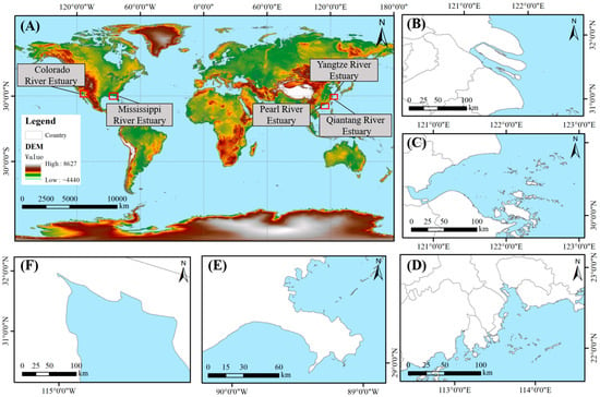
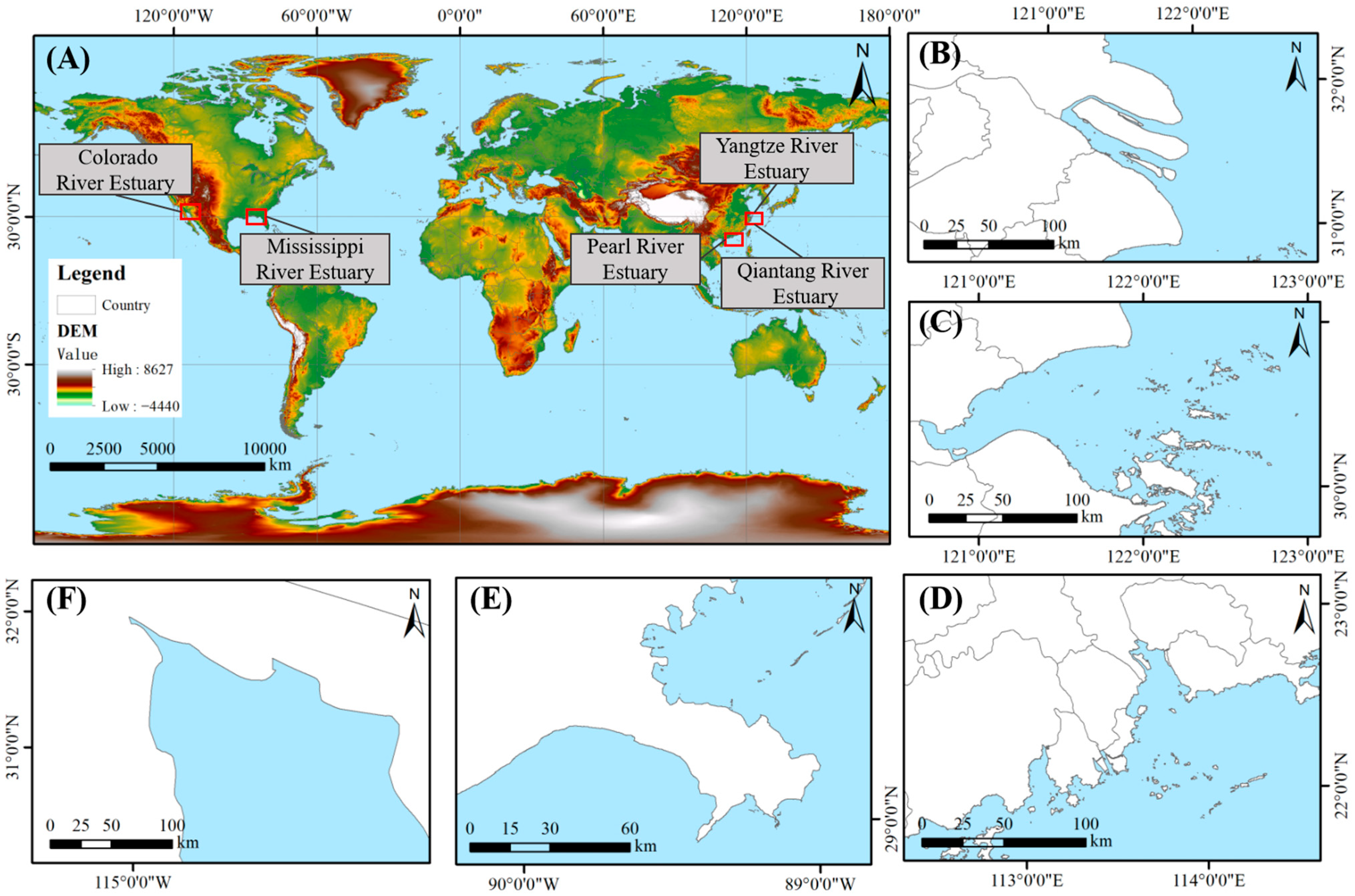
To systematically test the proposed framework across different hydrodynamic environments, this study selects five estuaries with contrasting hydro-climatic conditions (Figure 1). This selection is not arbitrary. These five estuaries form a gradient design covering two core controlling dimensions of front formation: the relative strength of river discharge versus tides, and the background water turbidity level.
Figure 1.
Distribution map of the study areas ((A) Geographic distribution of the estuaries, (B) Yangtze River Estuary, (C) Qiantang River Estuary, (D) Pearl River Estuary, (E) Mississippi River Estuary, (F) Colorado River Estuary).
The Yangtze River Estuary receives abundant river discharge and moderate tides, with a pronounced turbidity maximum zone [37]. Fronts frequently occur at the interface between salt and fresh water and in the transition zone between high- and low-suspended sediment concentrations, representing a river-dominated, high-turbidity estuarine type. The Pearl River Estuary has abundant river discharge but weak tides, with dense river networks and strong sediment deposition, representing a river-dominated, medium-turbidity estuarine type. The Qiantang River Estuary is famous for its strong tidal bore, characterized by low river discharge but strong tidal forcing, with flood tides dominating sediment transport and causing intense bed erosion and deposition [38], representing a tide-dominated, high-turbidity estuarine type. The Mississippi River Estuary exhibits abundant river discharge and weak tides, with highly stratified salt-freshwater mixing [39] and a delta that extends significantly seaward, representing a river-dominated, low-turbidity estuarine type. The Colorado River Estuary is located in the arid zone of northwestern Mexico, where river discharge has sharply decreased due to upstream water diversion projects [40]. Its turbidity fronts are primarily controlled by tidal mixing and residual sediment transport, and it is best described as an arid-zone, low-turbidity estuarine system.
The five estuaries cover multiple combinations from river-dominated to tide-dominated regimes, from humid to arid zones, and from high to low sediment transport. The core intention of this design is to systematically evaluate the performance of the proposed method under different dynamic types and optical backgrounds. We identify the method’s strengths and limitations. In particular, we test under what conditions AlphaEarth embeddings provide gains and under what conditions they fail. This evaluation offers empirical references for future research.
2.2. Remote Sensing Data
The typical width of a turbidity front ranges from tens to hundreds of meters. This width demands remote sensing data with high spatial resolution to resolve the fine front structure. It also requires moderate spectral resolution to capture subtle changes in water optical properties. Based on this requirement, this study adopted the L2A surface reflectance product from the European Space Agency Sentinel-2 satellites. The Sentinel-2 constellation comprises two satellites. The revisit cycle is 5 days. Spatial resolutions include 10 m, 20 m, and 60 m. The 10 m resolution suffices to resolve the internal structure of sub-mesoscale fronts. The L2A product underwent atmospheric correction. It directly provides surface reflectance values.
To match the 10 m spatial resolution of the subsequent AlphaEarth embedding data and to preserve the richest possible spectral information, this study resampled all bands uniformly to 10 m. The image time range spans June to November 2023. This period covers summer to autumn. During this interval, water color characteristics in each study area remain relatively stable. Cloud cover is also relatively low. During data screening, we selected images with cloud cover below 15% for compositing based on the cloud cover condition of each study area. The cloud masking procedure relied on the QA60 band contained in the images. This procedure ensured that only valid observations entered the composite. The specific Sentinel-2 acquisition dates for each study area are listed below.
- Yangtze Estuary: Two scenes (8 and 16 August 2023).
- Qiantang Estuary: Two scenes (24 and 26 November 2023).
- Pearl River Estuary: Two scenes (21 and 28 September 2023).
- Mississippi Estuary: One scene (9 September 2023).
- Colorado Estuary: One scene (19 October 2023).
For the first three estuaries, we mosaicked two scenes because a single scene could not fully cover the target area, either due to the large extent or cloud cover.
From the Sentinel-2 data, we extracted 11 spectral bands (B1~B8A, B11, B12) as the base spectral features. These bands cover the absorption and scattering properties of visible light by water (B2~B4). They also capture the response of suspended sediment concentration changes in the red and near-infrared bands (B4, B8). These features provide the fundamental spectral discriminants for front identification.
2.3. AlphaEarth Foundations Embedding Data
Traditional front identification methods rely on spectral and local statistical features. Their receptive field is limited to hundreds of meters around the target pixel. These methods cannot perceive whether an estuary is river-dominated or tide-dominated. They also fail to distinguish whether a turbid patch belongs to a front or constitutes a uniform mudflat. To overcome this limitation, this study introduces the 64-dimensional embedding vectors generated by the AlphaEarth Foundations [25]. Each 10 m pixel embedding vector does not represent a direct physical measurement or a retrieved parameter product. Instead, the model produces this vector as a high-dimensional semantic abstraction after fusing multi-source data [25]. Because the pre-training task reconstructs global land cover, the AlphaEarth embedding vectors have internalized a set of geospatial priors.
This study obtains and uses the AlphaEarth embedding data corresponding to the year 2023. Each pixel stores its embedding as a 64-dimensional vector. The data become available as an image collection on the Google Earth Engine platform. This format facilitates pixel-wise precise matching and fusion with the Sentinel-2 data.
2.4. Sample Point Construction
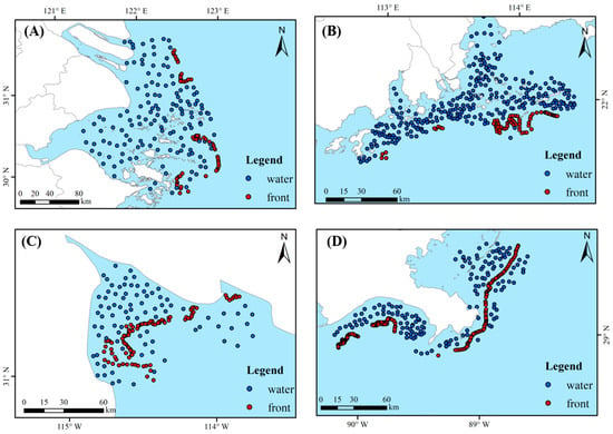
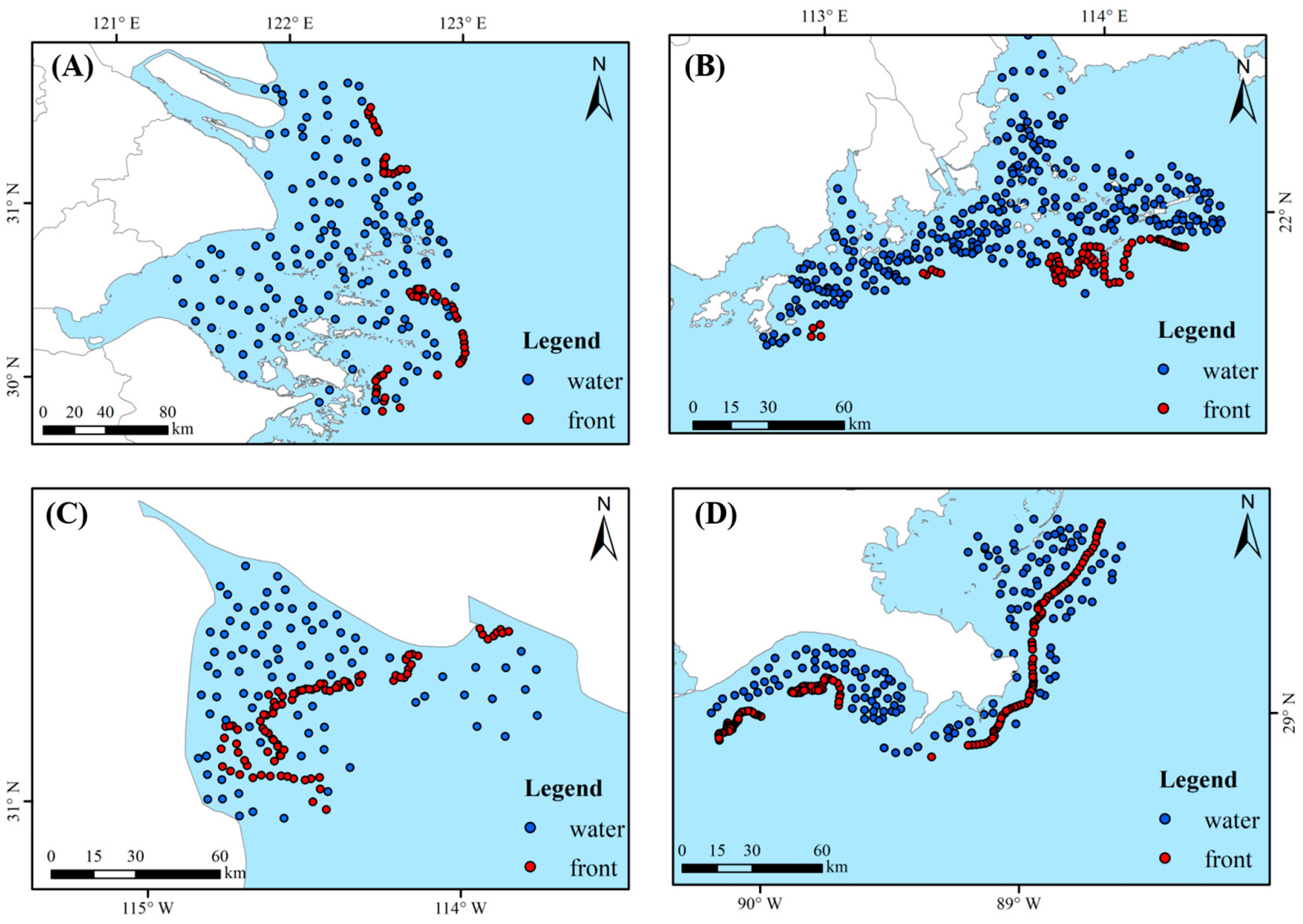
We constructed a dataset of 1055 sample points (Figure 2). Positive samples lie on turbidity fronts. Negative samples lie in uniform water bodies away from fronts (non-front areas). Labeling combined visual interpretation and multi-source data [41]. Candidate point locations for each estuarine region were first jointly determined by two researchers through examining Sentinel-2 true-color, NDWI, and red-band images [42]. Subsequently, each researcher independently classified every candidate point as either front or non-front water. The agreement rate between the two researchers’ independent annotations reached 94.3%, indicating high labeling consistency. Disputed samples underwent arbitration using high-resolution imagery and the literature. The labeling process excluded AlphaEarth embeddings and multi-scale statistics. This avoidance prevented accuracy inflation from information homogeneity. Sample distributions across the five estuarine regions are detailed in Table 1.
Figure 2.
Distribution map of sample points ((A) Yangtze River Estuary and Qiantang River Estuary, (B) Pearl River Estuary, (C) Colorado River Estuary, (D) Mississippi River Estuary).
Table 1.
Sample distribution across estuarine regions.
Samples spatially covered all five estuaries. Negative samples spanned different optical backgrounds including high-turbidity uniform areas, low-turbidity offshore waters, and clear zones. We discarded samples with cloud shadows, sun glint, or land-boundary mixed pixels [43] to ensure reliable optical signals for model training. A two-tier validation strategy was used to evaluate model generalization. The first tier was within-estuary validation. To avoid spatial leakage, we adopted a spatially stratified block-wise split based on a latitude–longitude grid. Specifically, all sample coordinates were first transformed from geographic coordinates to the Universal Transverse Mercator (UTM) projected coordinate system, and the study area was then divided into regular grid cells of 500 m × 500 m in the projected coordinate system. Each sample was assigned to a unique grid cell according to its projected coordinates. All grid cells were randomly partitioned into a training set (70%) and a validation set (30%), with the constraint that all samples within the same grid cell must belong entirely to the same dataset. This block-wise strategy ensured that no two spatially adjacent samples with a distance of less than 555 m appeared in different sets, thereby preventing overestimation of model performance due to spatial autocorrelation. The second tier was cross-estuary validation. We performed leave-one-estuary cross-validation, sequentially treating each estuary as an independent test set from which no training samples were taken, while the remaining four estuaries provided training data. This design explicitly tested cross-region generalization without any spatial or environmental overlap between the training and testing data.
3. Methodology
3.1. Technical Architecture
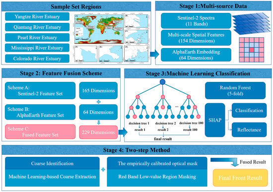
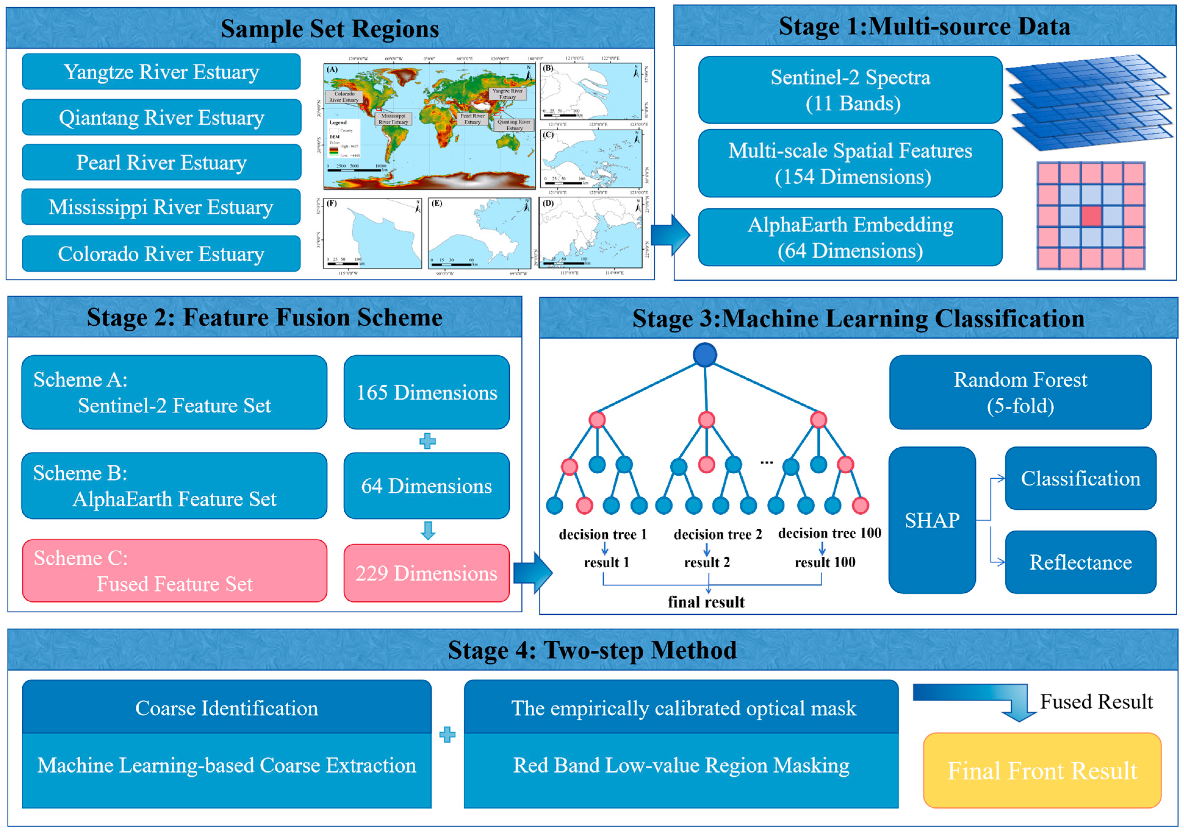
As stated in the introduction, traditional methods face three problems: non-transferable gradient thresholds, domain shift in supervised learning, and physical disconnection in data-driven models. To explore technical pathways addressing these three challenges, this study proposes a two-step synergistic method. This method decouples the front identification task into two sequential stages: high-recall extraction and high-precision verification (Figure 3). The core design principle assigns machine learning the role of capturing complex non-linear patterns from high-dimensional features. An empirically calibrated optical mask provides an additional constraint under turbid-estuary conditions. This method aims to improve identification accuracy and physical consistency within a single estuary. Section 5.3 describes how cross-region generalization performance was systematically tested and diagnosed.
Figure 3.
Flowchart of the proposed methodology.
Step one performs high-recall extraction using a data-driven approach. A random forest classifier receives the 229-dimensional fused feature tensor. The classifier generates a front probability map. Prioritizing sensitivity, this stage captures all possible front pixels, even at the cost of some false alarms. This design addresses the non-transferable threshold problem. The classifier learns from multi-scale statistical patterns instead of relying on a single gradient threshold.
Step two performs high-precision verification via an optical post-processing procedure. We intersect the candidate front pixels from step one with an optical mask derived from the Sentinel-2 red band (B4). The basis is that estuarine turbidity fronts almost invariably separate turbid water (low red-band reflectance) from relatively clear water (higher red-band reflectance). This step acts as a spatial logical AND gate. It removes any candidate pixels falling outside the low red-band reflectance zone. This design addresses the above limitation. Even if the machine learning model produces overly extended candidate frontal regions, the empirically calibrated optical mask prunes them in a “crude but correct” manner.
The two-step method offers complementary advantages. The machine learning component guarantees a high detection rate (recall). The empirically calibrated optical mask component guarantees high confidence (precision). Their synergy ensures that the final output possesses both the flexibility of a data-driven model and adherence to the basic definition of a front.
3.2. Feature Engineering
This section details the construction logic of the 229-dimensional feature set used in step one (high-recall extraction). Three feature types—spectral features, multi-scale spatial features, and AlphaEarth embedding features—form a complementary information structure.
3.2.1. Spectral Features
We extract surface reflectance of 11 bands (B1~B8A, B11, B12) from Sentinel-2 data as the base spectral features. These bands cover water absorption and scattering properties of visible light (B2~B4). They also capture the response of suspended sediment concentration changes in the red and near-infrared bands (B4, B8). A fundamental ambiguity exists in single-pixel spectra. A pixel at the center of a uniform high-turbidity zone and a pixel on the turbid side of a front may appear spectrally identical [43]. Therefore, spectral features must combine with spatial features.
3.2.2. Multi-Scale Spatial Features
Traditional gradient operators rely on fixed windows and a single threshold. They struggle to adapt to front widths ranging from tens to hundreds of meters in estuaries. To address this issue, we adopt a multi-scale kernel statistics approach [42,44]. This approach explicitly encodes the spatial context of fronts into the feature space. For each band, we compute the local mean and standard deviation under seven window sizes (3 × 3 to 15 × 15). The mean reflects the average spectral level of the neighborhood. The standard deviation characterizes spectral heterogeneity. The standard deviation peaks when the window straddles both sides of a front. Small windows (3 × 3, 5 × 5) remain sensitive to fine gradients at front edges. Large windows (13 × 13, 15 × 15) capture the macroscopic transition trend of fronts. This procedure yields a 154-dimensional spatial feature set (11 bands × 7 windows × 2 statistics). The classifier then learns the typical morphology of front transition zones from multi-scale statistical patterns, thus avoiding the non-transferable threshold problem.
3.2.3. AlphaEarth Embedding Features
As noted in Section 2.4, the AlphaEarth embedding represents a 64-dimensional high-level semantic vector. Its pre-training task reconstructs global land cover. Based on this pre-training mechanism, we propose a core hypothesis. In the 64-dimensional AlphaEarth embedding space, real fronts (linear transition boundaries) and artifact patches (e.g., uniform turbidity zones, algal bloom patches, bottom reflectance) may have spontaneously formed separable clusters. If this hypothesis holds, using AlphaEarth embeddings as an additional feature source should provide discriminative information that traditional spectral–spatial features lack. This information proves especially valuable for distinguishing land cover types with similar spectra but different spatial contexts.
3.2.4. Feature Fusion Scheme
To validate the independent contributions and synergistic effects of the three feature types, we design three comparison schemes.
Scheme A (Sentinel-2 baseline) uses 11 spectral bands plus 154 multi-scale spatial features (165 dimensions total). This scheme represents a baseline method combining traditional optical remote sensing data with spatial context information.
Scheme B (AlphaEarth only) uses the 64-dimensional AlphaEarth embedding features. This scheme evaluates the performance of a single foundation model embedding feature in the front identification task.
Scheme C (fusion) concatenates Scheme A and Scheme B (229 dimensions). The design of Scheme C follows the principle of complementarity. Spectral features provide pixel-scale physical measurements. Multi-scale spatial features provide geometric transition information of fronts. AlphaEarth embeddings provide the semantic context of the global geographic space. The combination of the three aims to address three challenges simultaneously. These challenges are non-transferable thresholds (handled by multi-scale features), feature complementarity validation (handled by AlphaEarth embeddings), and physical disconnection (handled by the empirically calibrated optical mask step).
Comparing Scheme A and Scheme C can test whether AlphaEarth embeddings provide information complementary to spectral–spatial features, while comparing Scheme B and Scheme C can test whether the fusion produces synergistic gains outperforming the simple addition.
3.3. Coordination Mechanism
3.3.1. Random Forest Classifier
To ensure objective model evaluation and spatial generalization, we first divided the dataset into non-overlapping spatial blocks based on latitude and longitude coordinates. We then split these blocks into a training set (70% of blocks) and a validation set (30% of blocks). We emphasize that the 30% validation set served only as a hold-out test set for final generalization performance. It did not participate in any model training, hyperparameter tuning, or early stopping. This strictly prevented spatial information leakage.
For the random forest model, we performed hyperparameter tuning using a grid search strategy. We restricted this search strictly to the 70% training set. We used spatial-block-based 5-fold cross-validation to evaluate the generalization error of different parameter combinations. The selection criterion was the average AUC across the cross-validation folds. The full search space included: n_estimators ∈ {50, 100, 200, 300}; max_depth ∈ {10, 15, 20, 30, None}; min_samples_leaf ∈ {1, 2, 4, 8}; max_features ∈ {‘sqrt’, ‘log2’, 0.3}; and class_weight ∈ {None, ‘balanced’}. The optimal parameter combination was n_estimators = 300, max_depth = 20, min_samples_leaf = 2, max_features = ‘sqrt’, and class_weight = ‘balanced’. After selecting the optimal parameters, we retrained the final model on the entire training set (70% of data) using these parameters. We then computed the classification performance on the independent validation set (30% of data). We fixed the random seed for all models at random_state = 42 to ensure reproducibility. We evaluated model performance using six metrics: accuracy, precision, recall, F1 score, the Kappa coefficient, and ROC-AUC.
To validate the suitability of random forest for this task, we further introduced XGBoost and a lightweight deep learning model (CNNTransformer) as comparative classifiers. XGBoost uses a tree-based ensemble strategy. It effectively handles non-linear interactions among high-dimensional features. We fixed its hyperparameters based on preliminary experiments: n_estimators = 100, max_depth = 6, learning_rate = 0.1, subsample = 0.8, colsample_bytree = 0.8, and random_state = 42. CNNTransformer combines convolutional neural networks and Transformer architectures. It captures local spatial features and global contextual associations. We trained it using the AdamW optimizer. We set the learning rate to 0.001 and the weight decay coefficient to 0.001. The batch size was 64. We trained for 500 epochs. To avoid information leakage from the 30% independent validation set, we did not use this 30% data for early stopping during CNNTransformer training. Instead, we directly output the model after the fixed training epochs. Its final evaluation also used only the independent 30% data. All comparative models adopted the same spatial-block partitioning strategy as the random forest. This ensures fair horizontal comparison and spatial independence.
3.3.2. Empirically Calibrated Optical Mask
The random forest model achieves high recall. However, its predictions may be over-extended in terms of candidate frontal area. Uniform high-turbidity zones present a typical case. The model tends to misclassify the entire region as a front. This behavior occurs because the training samples exhibit high collinearity between fronts and turbid water. The model mistakenly learns turbidity as a front signature. We binarized the random forest probability output using the default 0.5 threshold to obtain the binary front mask .
To suppress such false alarms, we introduced a empirically calibrated optical mask based on red-band reflectance (B4). The physical basis lies in strong absorption and backscattering of red light by suspended particles [45,46,47,48]. The key point is that the physical definition of a front requires spatial juxtaposition of turbid and clear water. A uniform turbid zone lacks this juxtaposition. The algorithm thus does not identify it as a front.
A Mann–Whitney U test on the 1055 labeled samples [49,50] quantitatively confirmed this physical pattern. Front pixels showed a median red-band reflectance of 0.0150. Non-front water pixels showed a median of 0.0375 (p < 0.001). Based on this result, we defined an optical mask, M_phys. A pixel remained a front candidate only if B4 < τ. The calibration of the threshold τ used the Youden index method [22] on the B4 histograms of each estuary mouth. The procedure yielded a global recommended value τ = 0.0289 for Sentinel-2 surface reflectance. It should be emphasized that this threshold is an empirically derived value based on the specific study areas and the specific sensor (Sentinel-2 L2A product). It is not a universal optical constant of water scattering. Therefore, we define this operation as an “empirically calibrated optical mask” rather than a universal physical law. The final front mask becomes:
where represents the front mask predicted by the random forest, and represents the empirically calibrated optical mask based on red-band reflectance (B4 < τ).
This logical AND operation grants a “veto power” to empirical statistical patterns. No matter how high the prediction confidence from the machine learning model, a pixel failing the low red-band condition faces exclusion from the final front. This directly addresses the physical disconnection dilemma, ensuring that the output conforms to the basic physical definition of a turbidity front.
To evaluate the sensitivity of this empirical optical mask to threshold variations, we set floating intervals of ±10% and ±20% around τ0 (0.8τ0, 0.9τ0, 1.1τ0, 1.2τ0) and performed a quantitative sensitivity test.
3.4. SHAP Feature Attribution and AlphaEarth Embedding Compression
We used SHAP to analyze how AlphaEarth 64-dimensional embeddings contribute to front detection. SHAP also helped us assess whether we could compress these embeddings. SHAP builds on Shapley values from game theory. It provides a consistent importance measure for each feature. This measure avoids the bias of Gini importance when features are correlated.
We pursued two related goals with SHAP. The first goal identified which embedding dimensions matter most for front classification. We trained a random forest classifier. The target variable was the front/non-front label. The features were the 64 AlphaEarth embeddings. We adopted a nested feature selection strategy. In the outer loop, we separated the training set (70%) from the validation set (30%) using spatial blocks. Inside the training set, we performed 5-fold cross-validation. In each fold, we trained the model on four subsets. We computed SHAP values on the remaining subset. We then averaged the mean absolute SHAP values across the five folds. This average became the classification importance score for each dimension. The random forest used the same hyperparameters as those described in Section 3.3.1.
The second goal examined which embedding dimensions link to Sentinel-2 optical reflectance. The 64 AlphaEarth dimensions do not directly represent known physical variables. Their meanings are not directly readable from the model. Therefore, we trained random forest regression models. The targets were Sentinel-2 band reflectance. We used the same nested spatial cross-validation framework. We computed the average absolute SHAP value of each embedding dimension for reflectance prediction. This analysis helped us separate two types of dimensions. Some dimensions have high SHAP for reflectance. They tend to encode information that overlaps with spectral data. Other dimensions have low SHAP for reflectance but high SHAP for classification. These may encode spatial context that spectral features cannot provide. The only difference between the two analyses was the target variable. For regression, we set n_estimators = 100 and max_depth = 10.
Based on the two SHAP analyses, we selected the top 20 dimensions with the highest average absolute SHAP values. These form two compressed subsets. One is “Classification-important Top20”. The other is “Reflectance-correlated Top20”. We then compared their classification performance on the same spatial-block validation set. This comparison told us which compression strategy works better. We implemented all SHAP computations using TreeExplainer.
4. Results and Analysis
4.1. Synergistic Gains of Feature Fusion
To test whether multi-source feature fusion produces synergistic gains, and to validate the suitability of different classifiers, we compared three models (random forest, XGBoost, and CNNTransformer) across three feature schemes (Table 2). The results show that random forest consistently outperforms XGBoost and CNNTransformer in both F1 score and AUC under all feature schemes. As a boosting ensemble, XGBoost faces a certain overfitting risk with high-dimensional features. CNNTransformer, limited by a moderate-sized training set, cannot fully exploit its representation potential. Random forest, with its bagging strategy, shows good robustness to high-dimensional features and strong resistance to overfitting. It achieves the best balance in this task. Therefore, we used it as the base classifier for all subsequent experiments.
Table 2.
Classification performance comparison across feature schemes and models.
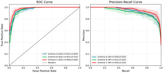
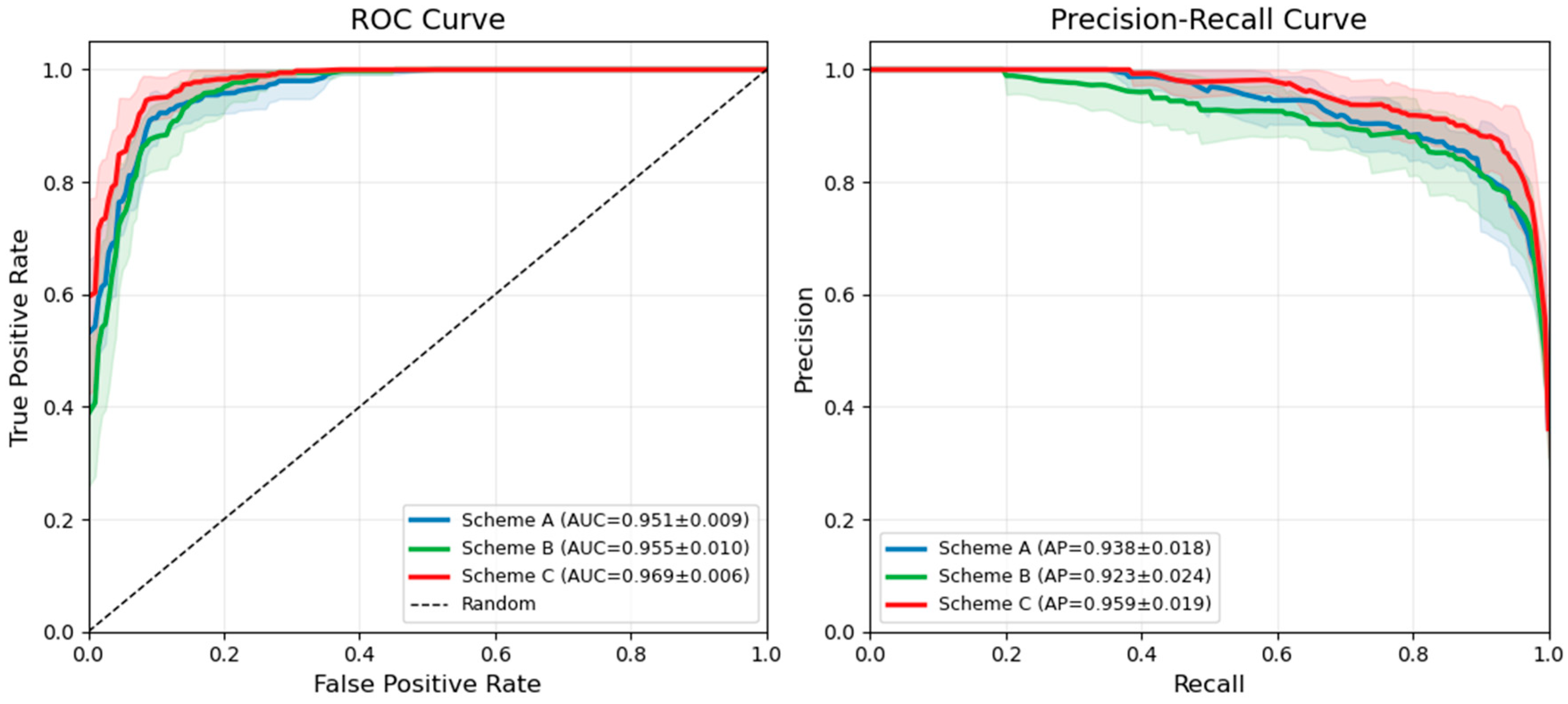
First, Scheme B (AlphaEarth alone) yields an accuracy of 87.3%, slightly lower than that of Scheme A (87.7%), with notably lower recall and F1 score. This result suggests that AlphaEarth embeddings alone offer limited effectiveness as independent classification features. The embeddings encode abstract semantics rather than directly discriminable spectral information, leading to a precision-oriented but recall-limited performance. Second, Scheme C (fusion) outperforms both Scheme A and Scheme B across all metrics. Compared to Scheme A, accuracy increases by 3.5 percentage points, recall increases by 6.4 percentage points, and F1 score improves from 0.824 to 0.875. Compared to Scheme B, the improvements are even more substantial: accuracy increases by 3.9 percentage points, recall increases by 10.0 percentage points, and F1 score improves by 0.058. Third, the fused scheme achieves an AUC of 0.969, higher than that of both Scheme A and Scheme B, indicating excellent discriminative ability of the classifier. The ROC and precision–recall curves (Figure 4) further confirm this improvement. Scheme C consistently maintains a higher curve position than the other two schemes, achieving the largest AUC values in both ROC and PR spaces, which indicates stronger overall separability and more stable recognition performance.
Figure 4.
ROC and precision–recall curves of different feature schemes.
The core insight from these results lies in the complementary rather than redundant relationship between AlphaEarth embeddings and spectral–spatial features. Scheme B performs poorly in recall (79.1%) when used alone. Adding it to Scheme A, however, produces significant synergistic gains: recall increases from 82.7% to 89.1%, and F1 score improves from 0.824 to 0.875. This outcome precisely confirms our core hypothesis from the introduction. The global semantic prior provided by AlphaEarth embeddings requires combination with local spectral–spatial features to realize its true value. The substantial recall improvement in the fusion scheme demonstrates that multi-scale spatial features, when enhanced by AlphaEarth embeddings, effectively solve the problem of missed front edges caused by mixed pixels.
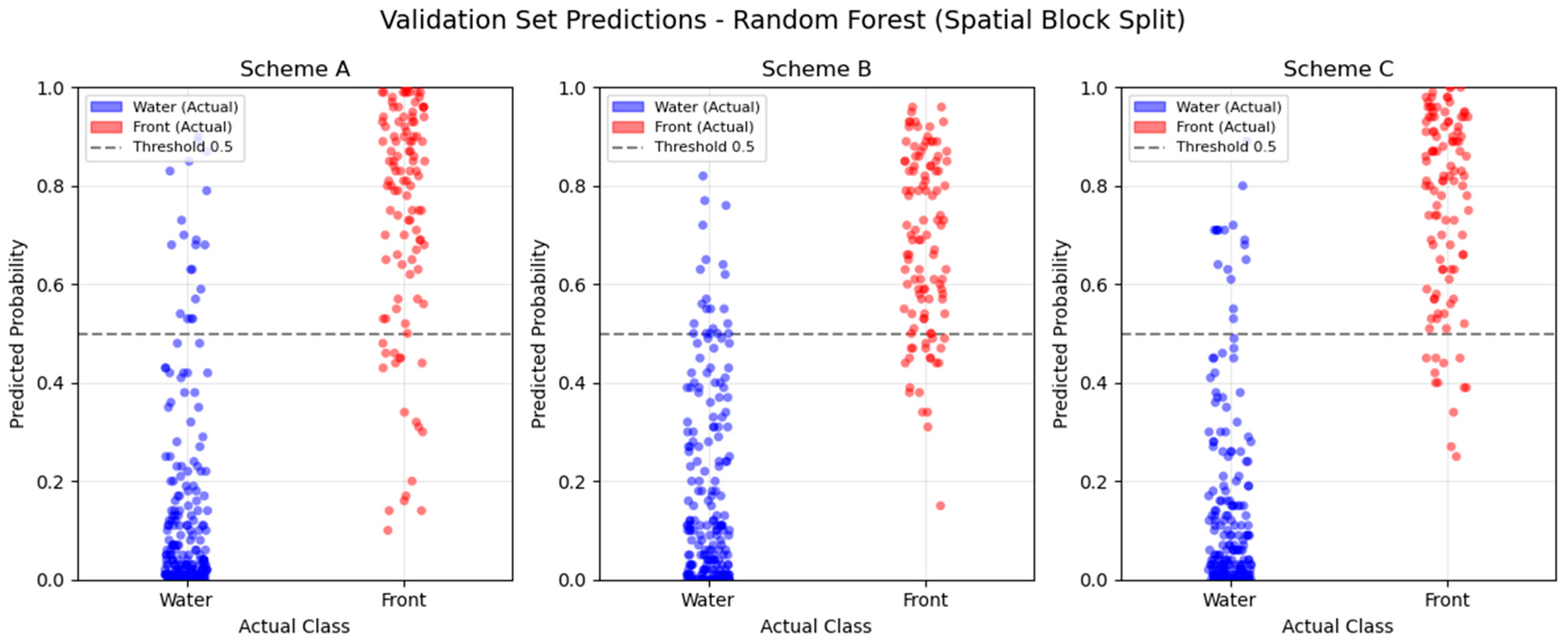
Figure 5 shows the predicted probability distributions of the three schemes on the validation set. In Scheme A, water sample probabilities mostly fall below 0.2. Front sample probabilities, however, show a scattered distribution, with some values near 0. In Scheme B, front sample probabilities concentrate in the 0.5~0.8 range, failing to reach a high confidence level. In Scheme C, water sample probabilities stay below 0.2. Front samples almost all lie above 0.7. The separation between the two sample types expands significantly, and the dispersion reduces markedly. This visualization confirms the discriminative advantage of the fused features from a probability distribution perspective.
Figure 5.
Scatter plot of classification probabilities for different feature combination schemes.
4.2. Statistical Basis and Threshold Sensitivity of the Optical Mask
To reduce the areal false alarms that the random forest model may produce in uniformly turbid zones, we constructed an empirical optical mask based on red-band (B4) reflectance. This section first examines the statistical basis of this mask and then evaluates its sensitivity to threshold variations.
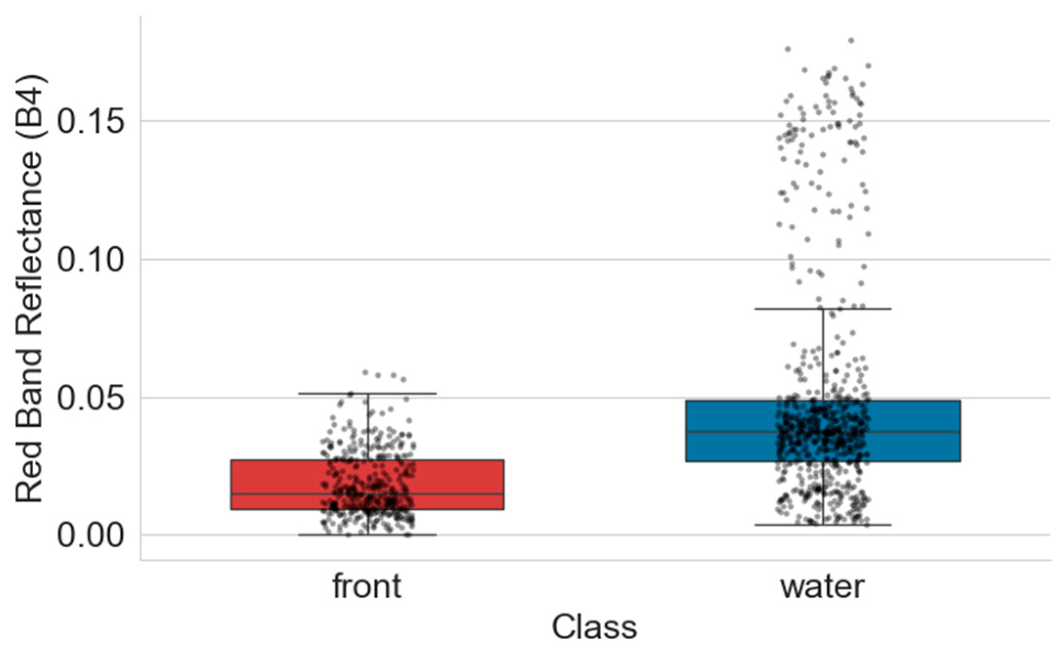
We first performed a Mann–Whitney U test on the red-band reflectance of the 1055 labeled samples (Figure 6, Table 3).
Figure 6.
Boxplot of red band reflectance for front vs. non-front water bodies.
Table 3.
Statistical summary of red band reflectance for front and non-front water bodies.
The results show that front samples have significantly lower mean (0.0183) and median (0.0150) red-band reflectance than non-front water samples, with a p-value less than 0.001 from the Mann–Whitney U test. Based on this, we used the Youden index method from the ROC curve on the local training samples to calibrate an initial threshold τ0 = 0.028975, and constructed the empirical optical mask as B4 < τ0.
To evaluate the sensitivity of this empirical optical mask to threshold selection, we set floating intervals of ±10% and ±20% around τ0 (i.e., 0.8τ0, 0.9τ0, 1.1τ0, 1.2τ0), and recorded the accuracy, precision, recall, F1 score, IoU, and false positive pixel counts under different thresholds (Table 4).
Table 4.
Sensitivity analysis results under different red-band threshold settings.
When the threshold varies within ±20% of τ0, the F1 score remains between 0.674 and 0.700, and the IoU stays between 0.509 and 0.539. This indicates that the empirical optical mask is reasonably robust to threshold fluctuations. However, deviating from the optimal threshold brings clear performance trade-offs. When the threshold increases to 1.2τ0, recall rises to 0.8976, but precision drops to 0.5490 (a decrease of 0.0717 from τ0). This suggests that an overly lenient threshold introduces many non-front uniform water pixels into the front candidates. When the threshold decreases to 0.8τ0, precision rises to 0.6567, but recall drops to 0.6929 (a decrease of 0.1102 from τ0), significantly increasing the risk of missing real fronts. These sensitivity results are consistent with the distribution patterns in Table 2. The 75th percentile of B4 reflectance for front samples (0.0274) is close to the optimal threshold τ0 (0.028975). The clear decline in either precision or recall when deviating from τ0 confirms that the Youden index-calibrated threshold achieves an optimal balance between missed detections and false alarms. Therefore, in practice, the optimal threshold τ0 calibrated by the Youden index should be used for front extraction to ensure reliable identification performance.
4.3. Application Effectiveness of the Optical Mask
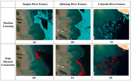
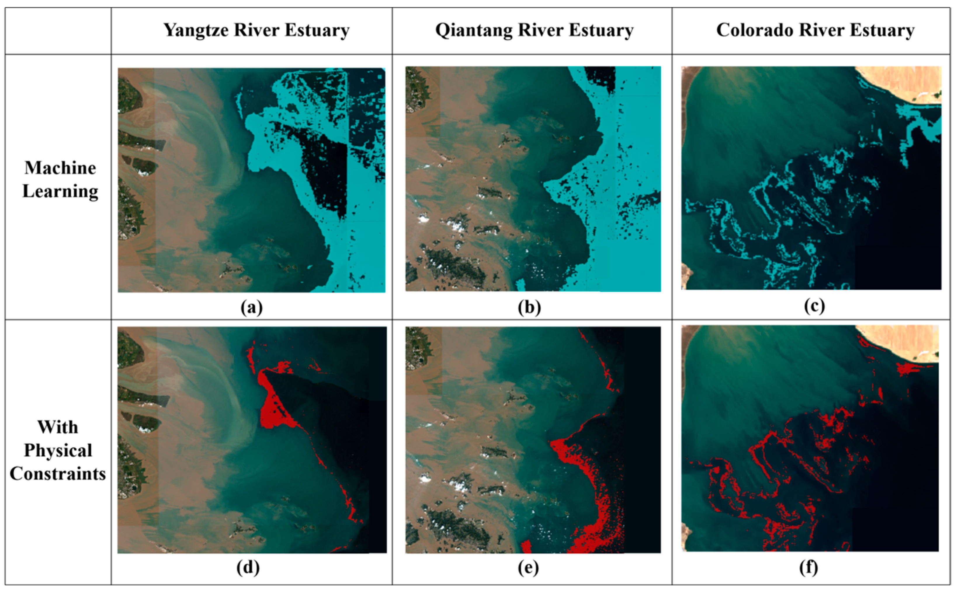
Using the optimal threshold τ0, this section evaluates the refinement performance of the empirical optical mask for front identification. Figure 7 compares front identification results before and after applying the empirically calibrated optical mask. Three representative estuaries exhibited different mechanisms. These three estuaries represent three types: river-dominated high turbidity (Yangtze River Estuary), tide-dominated high turbidity (Qiantang River Estuary), and tide-dominated low turbidity (Colorado River Estuary).
Figure 7.
Comparison of turbidity front identification results in typical estuaries.((a) Yangtze River Estuary without physical constraints; (b) Qiantang River Estuary without physical constraints; (c) Colorado River Estuary without physical constraints; (d) Yangtze River Estuary with physical constraints; (e) Qiantang River Estuary with physical constraints; (f) Colorado River Estuary with physical constraints).
In the Yangtze River Estuary (Figure 7a,d), the machine learning prediction alone generates overly extended candidate frontal regions. The entire turbidity maximum zone appears as a turbidity front. After applying the optical mask, the front shrinks into a clear striped pattern. This pattern closely matches the water color transition zone in the Sentinel-2 true-color image. The front extends southeastward from Nanhui Shoal [51]. Highly turbid water lies on the inner side. Relatively clear offshore water lies on the outer side.
The Qiantang River Estuary (Figure 7b,e) shows a similar pattern. The machine learning prediction alone yields overly extended candidate frontal regions. After the optical mask, the front reduces to a narrow strip. This strip faithfully delineates the path of the suspended sediment front under tidal dynamics. The path corresponds to the tide-dominated sediment transport route during the low-discharge season in November [52,53]. Quantitative statistics for the two estuaries show that the optical mask reduces the misclassified planar area by about 64.56% and 54.65%, respectively (from 4415.48 km2 to 1564.61 km2, and from 5451.97 km2 to 2472.42 km2). This case demonstrates the veto power of the optical mask. No matter how high the prediction confidence from the machine learning model, a pixel failing the low red-band condition—meaning it does not lie on a turbidity change boundary—faces exclusion from the final front.
The Colorado River Estuary (Figure 7c,f) presents a different situation. River discharge has sharply decreased in this estuary, limiting sediment supply. The overall water turbidity remains low. The machine learning prediction alone already produces a reasonable front pattern with a mix of strips and patches. The result after the optical mask closely matches the original prediction, with only minor edge refinement. This difference precisely verifies the design intention of the optical mask. The constraint intervenes only when the machine learning model generates areal false alarms. In low-turbidity environments where the model already performs well, the constraint serves to validate and refine rather than veto.
The above cases demonstrate the effectiveness of our method under different optical backgrounds. The model transfer performance across different estuaries represents a key test of generalization ability. Section 5.3 reports and diagnoses this performance systematically.
4.4. SHAP Feature Attribution and Embedding Compression
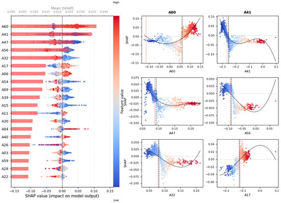
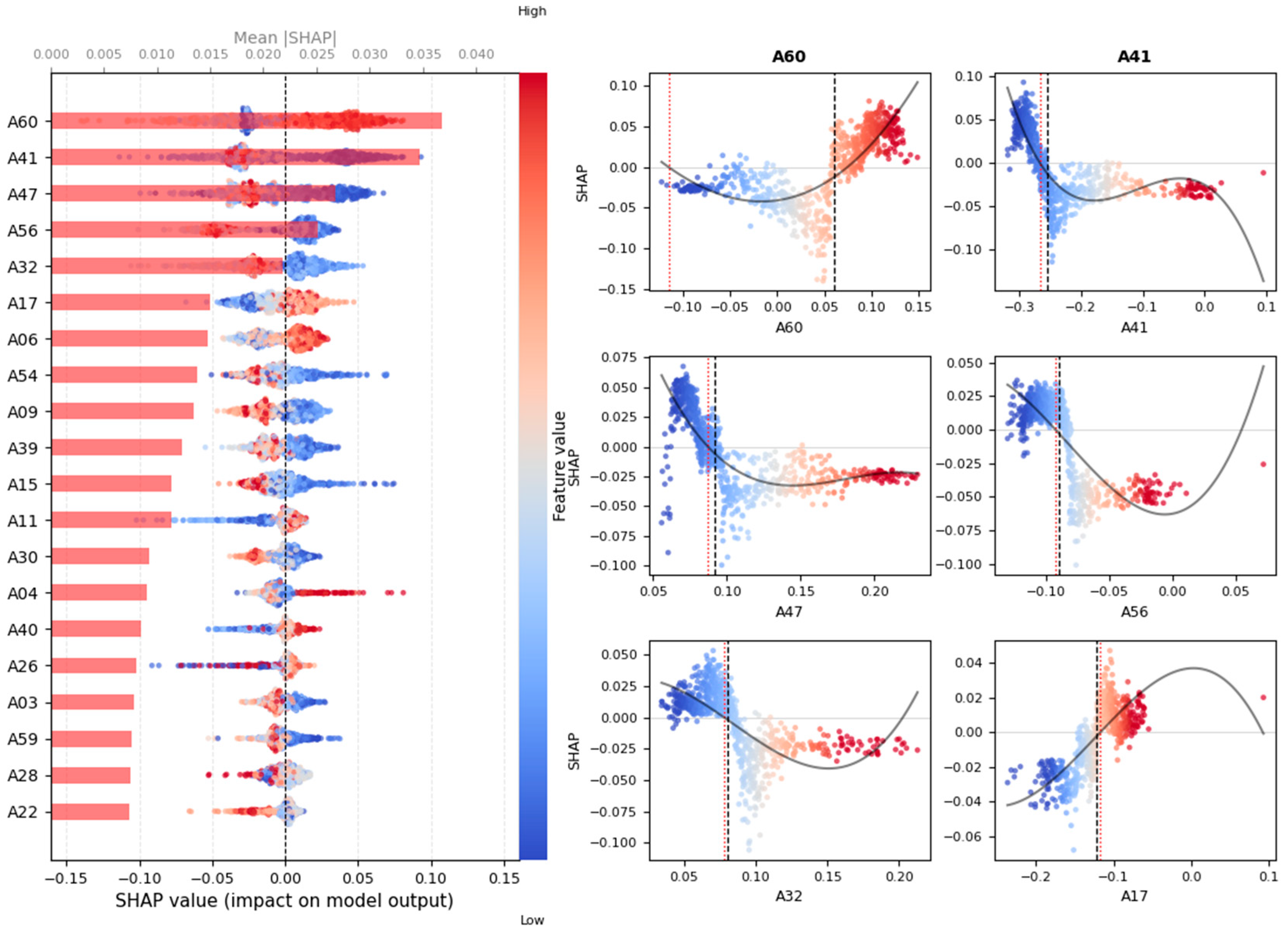
The classification SHAP analysis identifies the embedding dimensions that contribute most to estuarine front discrimination. It operates within the nested spatial cross-validation framework. The accuracy across the validation folds ranges from 0.816 to 0.919. This indicates that the model learns well within the training set and maintains good generalization on the inner validation sets. Figure 8 shows the top 20 embedding dimensions ranked by their SHAP importance for classification. Among them, A60, A41, A47, and A56 show significantly higher contributions than the rest. They form the first tier. A32, A17, A06, and A54 form the second tier. The remaining dimensions have relatively close contribution values. A60, A41, and A47 clearly stand above all others.
Figure 8.
SHAP-based importance ranking of the top 20 AlphaEarth embedding dimensions for front classification.
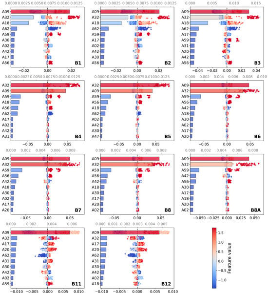
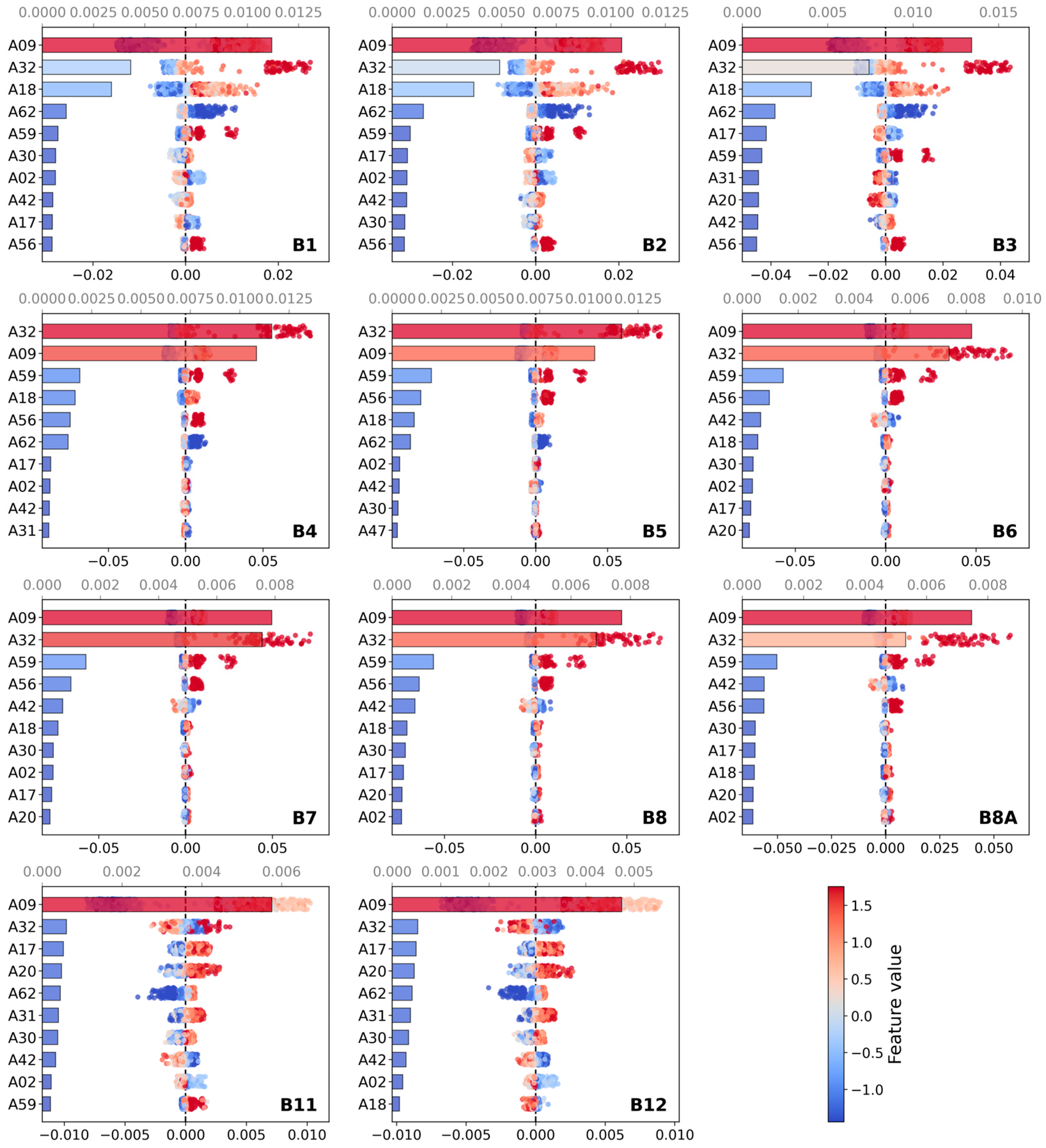
The reflectance prediction SHAP analysis uses the same nested spatial cross-validation framework. It examines the associations between AlphaEarth embeddings and Sentinel-2 optical reflectance. The average R2 across the five folds is 0.8506. The average MAE is 0.0048. The average RMSE is 0.0094. Figure 9 shows the mean absolute SHAP values of each embedding dimension for predicting Sentinel-2 band reflectance. The color intensity indicates the contribution level. Across all bands, the reflectance-correlated Top20 consists of: A09, A32, A18, A59, A56, A62, A42, A17, A30, A02, A20, A31, A47, A53, A24, A41, A35, A05, A36, and A33. Among them, A09 and A32 far exceed the others in contribution. They form the absolute dominant tier. A18, A59, A56, and A62 form the second tier. The remaining dimensions all show low contributions, with an order-of-magnitude gap from the first tier.
Figure 9.
Mean absolute SHAP values of AlphaEarth embedding dimensions for predicting Sentinel-2 band reflectance (B1–B12).
Comparing the composition of the two Top20 lists, only nine dimensions appear in both lists. They are A41, A47, A56, A32, A17, A06, A09, A30, and A59. The overlap ratio is less than half. The ranking positions also differ significantly. A60 does not enter the Top20 for reflectance prediction, but ranks first in the classification SHAP. A09 ranks first in the reflectance prediction, but only ranks ninth in the classification SHAP. A41 ranks sixteenth in the reflectance prediction, but ranks second in the classification SHAP. This result shows that the dimensions that contribute most to optical reflectance are not the same as those that contribute most to front discrimination. The two sets encode different types of information within the embedding space.
Table 5 compares the classification performance of the full AlphaEarth embeddings and the two Top20 compression schemes on the spatial-block validation set. The full 64-dimension embedding achieves an F1 of 0.842. The reflectance-correlated Top20 achieves an F1 of 0.8507 after compression. This slightly outperforms the full 64-dimension set, suggesting that removing redundant dimensions reduces overfitting to some extent. The classification-important Top20 achieves an F1 of 0.8125. Both Top20 subsets are selected under the same nested framework. Their performance difference reflects the different utility of spectral information versus task-specific information in the embedding space for estuarine front classification.
Table 5.
Classification performance of different embedding feature subsets.
5. Discussion
5.1. Synergistic Mechanism of Feature Fusion
As reported in Section 4.1, AlphaEarth embeddings alone yield a classification accuracy of 87.3%. This value falls below the 87.7% achieved by Sentinel-2 spectral–spatial features alone. Fusing the two, however, raises the accuracy to 91.2%. This counter-intuitive synergistic gain does not represent simple addition. Instead, it results from information complementarity.
Spectral features (11 dimensions) provide pixel-scale physical measurements. Their inherent ambiguity, however, prevents them from distinguishing a uniform high-turbidity zone from a front edge. Multi-scale spatial features (154 dimensions) explicitly characterize the geometric property of a front as a transition zone possessing a finite width. Large-window standard deviations achieve this characterization. This information—the finite width of fronts—remains absent from single-pixel spectra [12,42,44].
AlphaEarth embeddings compensate for the missing macroscopic context in the first two feature types. The pre-training task implicitly encodes topological continuity, scale consistency, and contextual associations. Local Sentinel-2 data do not directly provide these priors.
This synergistic mechanism offers an important insight. Foundation models should not be treated as end-to-end classifiers (Scheme B performs poorly). Instead, they serve as feature enhancers. Their embedding vectors act as semantic priors orthogonal to local features. Fusing these priors with task-specific features maximizes their value. The prominent contribution of ten embedding dimensions in the feature importance analysis supports this conclusion empirically.
5.2. Validity Examination of the Empirically Calibrated Optical Mask
As Section 4.3 describes, the effectiveness of the low red-band empirically calibrated optical mask strongly depends on the optical contrast across the front. In estuaries with highly turbid river water (Yangtze River, Qiantang River) [48], the red-band reflectance difference between the two sides of a front reaches 0.03~0.05. The threshold τ = 0.028975 clearly separates fronts from uniform water bodies. The Mann–Whitney U test (p < 0.001) statistically confirms the significance of this difference [49,50]. The sensitivity analysis in Section 4.2 further shows that the F1 score remains stable between 0.674 and 0.700 when τ varies within ±20% of τ0, indicating reasonable robustness under the optical conditions of this study.
In low-turbidity estuaries (Colorado River Estuary), the situation differs. River diversion has reduced sediment input, making the overall water turbidity low [40]. Here, the empirical optical mask mainly refines edges.
This finding suggests that the optical masks must match the optical background of the target region. Future research could explore adaptive approaches that dynamically select the most sensitive band or index based on the regional optical background, rather than relying on a single fixed threshold.
5.3. Empirical Assessment of Cross-Estuary Transferability
The results in Section 4.1, Section 4.2 and Section 4.3 show that our method achieves high identification accuracy within the training estuary (random split validation) and between estuaries sharing similar optical backgrounds. A more fundamental question remains: does the model transfer reliably across estuaries with different dynamic regimes? To answer this question, we employ a leave-one-estuary cross-validation strategy. We sequentially treat each of the five estuaries as an independent test set, using the remaining four for training. Table 6 presents the results. We observed three patterns.
Table 6.
Leave-one-estuary cross-validation results.
The first level represents successful generalization. The Pearl River Estuary (F1 = 0.838) and the Qiantang River Estuary (F1 = 0.822) perform well. The training set contains estuaries with similar dynamic regimes. The Pearl River Estuary shares a river-dominated regime with the Yangtze River Estuary. The Qiantang River Estuary, as a tide-dominated high-turbidity estuary, still allows the model to learn its front morphology.
The second level represents partially successful generalization. The Mississippi River Estuary (F1 = 0.707) and the Colorado River Estuary (F1 = 0.532) show below-medium performance. The Colorado River Estuary, as an arid-zone low-turbidity tide-dominated estuary, differs markedly from the training set (dominated by river-driven high-turbidity estuaries). Its recall reaches only 42%.
The third level represents generalization failure. When the Yangtze River Estuary serves as the test set, the F1 score drops to 0.333. Analysis of the test samples from this estuary reveals that its front morphology is the most complex among the five estuaries. The turbidity maximum zone is well developed, and the fronts exhibit a multi-branched distribution. Consequently, the model cannot infer this unique structure from other estuaries. This case reveals a core challenge in cross-region transfer: when the target estuary possesses a front morphology lacking similar samples in the training set, the model generalization ability declines sharply.
These results indicate that foundation-model embeddings, while effective within similar optical regimes, do not guarantee robust cross-domain generalization. The observed performance degradation under domain shifts provides empirical constraints that should inform future model development and domain-adaptation strategies.
5.4. Implications for Embedding Compression
As noted in Section 4.4, only nine dimensions overlap between the classification SHAP Top20 and the reflectance prediction SHAP Top20. This raises a question. If AlphaEarth provides complementary information to local spectral features, which dimensions should we prioritize for compression? Should we keep the dimensions that matter most for classification, or those most correlated with reflectance? The two choices may lead to very different compression outcomes.
The two Top20 lists differ clearly. A60 ranks first in classification but contributes little to reflectance. A09 ranks first in reflectance but only ninth in classification. A41 ranks sixteenth in reflectance but second in classification. The most important dimensions for reflectance are not the same as those for front discrimination. The two tasks use different parts of the embedding space.
This difference likely comes from AlphaEarth pre-training. AlphaEarth uses diverse Earth observation data, including optical imagery and synthetic aperture radar. Some dimensions encode spectral information similar to Sentinel-2. Others encode spatial context, edge patterns, or topological information. These may come from other remote sensing data sources, not from single-pixel Sentinel-2 spectra. They represent the added value of foundation embeddings. Classification uses the latter dimensions. Reflectance prediction uses the former.
Regarding compression performance, Table 5 shows that the reflectance-correlated Top20 achieves an F1 of 0.8507. The classification-important Top20 achieves an F1 of 0.8125. The full 64-dimension set achieves 0.842. The advantage of reflectance-related dimensions suggests that spectral information contributes more directly to classification on the current dataset. However, the classification-important Top20 is selected under a nested framework with a fully isolated validation set. Its performance estimate is more conservative. It offers higher credibility for generalization to unseen estuaries.
Considering both dimension robustness and generalization needs, we recommend prioritizing the dimensions that both SHAP analyses identify as important. These nine dimensions are A41, A32, A09, A06, A59, A30, A56, A47, and A17. They relate to both water optical information and classification decisions. They represent the most robust core information within the embedding space. The full 64-dimension embedding is not necessarily the best choice. Proper compression can reduce computational and storage costs while improving generalization robustness.
6. Conclusions
This study introduces AlphaEarth Foundations embeddings into the estuarine turbidity front identification task for the first time. We construct a 229-dimensional cross-modal feature set that fuses spectral–spatial features with AlphaEarth embeddings. We also propose a two-step synergistic method of random forest prediction and low red-band empirically calibrated optical mask. Addressing the four scientific questions posed in the introduction, we draw the following conclusions.
- (i)
- The fused feature set yields significant synergistic gains within a single estuary. The overall accuracy reaches 91.2% and recall 89.1%. Ten AlphaEarth embedding dimensions enter the top 30 feature importance ranks. This result shows that these embeddings provide semantic information complementary to spectral–spatial features.
- (ii)
- The empirically calibrated optical mask effectively removes candidate frontal area in high-turbidity estuaries. In the Yangtze River and Qiantang River estuaries, the constraint reduces the planar misclassification area by approximately 59.09%. It restores the true linear morphology of fronts. The Mann–Whitney U test (p < 0.001) confirms the physical rule of low red-band reflectance in front zones.
- (iii)
- Leave-one-estuary F1 scores ranged from 0.33 to 0.84 across five estuaries. They were below the within-estuary score of 0.93. This shows limited cross-estuary generalization. It also suggests AlphaEarth embeddings are not domain-invariant. We identified three causes: sample bias, geographic dependence, and limited temporal sampling. These findings can inform domain-adaptation strategies.
- (iv)
- We offer clear recommendations for applying geospatial foundation models. AlphaEarth embeddings should act as feature enhancers fused with local spectral–spatial features, rather than standalone end-to-end classifiers. SHAP analysis reveals only nine overlapping dimensions between the two Top-20 lists, indicating a clear functional division within the embedding space. We recommend prioritizing these nine dimensions (A41, A32, A09, A06, A59, A30, A56, A47, A17), as they relate to both water optical information and classification decisions, while reducing computational cost and improving generalization robustness.
Future research should focus on domain adaptation strategies and multi-temporal sample collection [54]. The cross-estuary failures observed in this study underscore the need to develop targeted adaptation techniques and to build more diverse training datasets that cover a wider range of hydrodynamic regimes. These efforts will further improve model transfer robustness across different estuarine environments. Exploring adaptive empirically calibrated optical masks and lightweight foundation model adaptation also represents important directions for moving this method toward operational applications.
Author Contributions
Conceptualization, W.W. and F.S.; methodology, L.Y. and W.W.; software, L.Y. and Y.T.; validation, L.Y., Y.T. and P.Z.; formal analysis, L.Y. and H.J.; investigation, L.Y. and Y.T.; resources, W.W. and F.S.; data curation, Y.T.; writing—original draft preparation, L.Y. and W.W.; writing—review and editing, W.W., P.Z., H.J. and F.S.; visualization, L.Y.; supervision, W.W. and F.S.; project administration, W.W. and F.S.; funding acquisition, W.W. and F.S. All authors have read and agreed to the published version of the manuscript.
Funding
This work was supported by the Strategic Priority Research Program of the Chinese Academy of Sciences (Grant No. XDB0740300) and the National Natural Science Foundation of China (Grant No. 42576204).
Data Availability Statement
The data presented in this study are available on request from the corresponding author due to privacy restrictions, as well as the data being part of an ongoing research project.
Conflicts of Interest
The authors declare no conflicts of interest.
References
- Garvine, R.W.; Monk, J.D. Frontal structure of a river plume. J. Geophys. Res. 1974, 79, 2251–2259. [Google Scholar] [CrossRef] [Scilit]
- Belkin, I.M.; Cornillon, P.C.; Sherman, K. Fronts in large marine ecosystems. Prog. Oceanogr. 2009, 81, 223–236. [Google Scholar] [CrossRef] [Scilit]
- Klemas, V. Remote sensing of coastal plumes and ocean fronts: Overview and case study. J. Coast. Res. 2012, 28, 1–7. [Google Scholar] [CrossRef] [Scilit]
- Belkin, I.M. Remote sensing of ocean fronts in marine ecology and fisheries. Remote Sens. 2021, 13, 883. [Google Scholar] [CrossRef] [Scilit]
- Belkin, I.M.; O’Reilly, J.E. An algorithm for oceanic front detection in chlorophyll and SST satellite imagery. J. Mar. Syst. 2009, 78, 319–326. [Google Scholar] [CrossRef] [Scilit]
- Kirches, G.; Paperin, M.; Klein, H.; Brockmann, C.; Stelzer, K. GRADHIST—A method for detection and analysis of oceanic fronts from remote sensing data. Remote Sens. Environ. 2016, 181, 264–280. [Google Scholar] [CrossRef] [Scilit]
- Miller, P. Multi-spectral front maps for automatic detection of ocean colour features from SeaWiFS. Int. J. Remote Sens. 2004, 25, 1437–1442. [Google Scholar] [CrossRef] [Scilit]
- Mann, H.B.; Whitney, D.R. On a test of whether one of two random variables is stochastically larger than the other. Ann. Math. Stat. 1947, 18, 50–60. [Google Scholar] [CrossRef] [Scilit]
- Baaklini, G.; Brajard, J.; Issa, L.; Fifani, G.; Mortier, L.; El Hourany, R. Monitoring the coastal–offshore water interactions in the Levantine Sea using ocean color and deep supervised learning. Ocean Sci. 2024, 20, 1707–1720. [Google Scholar] [CrossRef] [Scilit]
- Cayula, J.F.; Cornillon, P. Edge detection algorithm for SST images. J. Atmos. Ocean. Technol. 1992, 9, 67–80. [Google Scholar] [CrossRef] [Scilit]
- Youden, W.J. Index for rating diagnostic tests. Cancer 1950, 3, 32–35. [Google Scholar] [CrossRef] [Scilit]
- Yu, J.; Guan, L. Research on Sea Surface Temperature Front Detection Algorithm Based on SNPP/VIIRS Satellite Data. Period. Ocean Univ. China 2024, 54, 21–29. [Google Scholar]
- Ulloa, N.I.; Choi, C.; Yeng, C.H.; Hill, E.M.; Yun, S.H. A SAR-based U-Net model for Coastal Monitoring: Global Pretraining and Localized Adaptation. In Proceedings of the 2025 International Conference on Machine Intelligence for GeoAnalytics and Remote Sensing (MIGARS), Hyderabad, India, 15–18 September 2025; pp. 1–4. [Google Scholar]
- Wan, X.; Zhang, L.; Ma, X.; Xu, W.; Chen, Q.; Zhao, R.; Zeng, M. Dynamic gradient orientation and multi-scale fusion network for ocean front detection. J. Sea Res. 2025, 206, 102601. [Google Scholar] [CrossRef] [Scilit]
- Xing, Q.; Yu, H.; Wang, H.; Yu, H. A sliding-window-threshold algorithm for identifying global mesoscale ocean fronts from satellite observations. Prog. Oceanogr. 2023, 216, 103072. [Google Scholar] [CrossRef] [Scilit]
- Felt, V.; Kacker, S.; Kusters, J.; Pendergrast, J.; Cahoy, K. Fast ocean front detection using deep learning edge detection models. IEEE Trans. Geosci. Remote Sens. 2023, 61, 1–12. [Google Scholar] [CrossRef] [Scilit]
- Reichstein, M.; Camps-Valls, G.; Stevens, B.; Jung, M.; Denzler, J.; Carvalhais, N.; Prabhat, F. Deep learning and process understanding for data-driven Earth system science. Nature 2019, 566, 195–204. [Google Scholar] [CrossRef] [Scilit] [PubMed]
- Castelvecchi, D. Can we open the black box of AI? Nature 2016, 538, 20. [Google Scholar] [CrossRef] [Scilit] [PubMed]
- Rudin, C. Stop explaining black box machine learning models for high stakes decisions and use interpretable models instead. Nat. Mach. Intell. 2019, 1, 206–215. [Google Scholar] [CrossRef] [Scilit] [PubMed]
- Karpatne, A.; Atluri, G.; Faghmous, J.H.; Steinbach, M.; Banerjee, A.; Ganguly, A.; Shekhar, S.; Samatova, N.; Kumar, V. Theory-guided data science: A new method for scientific discovery from data. IEEE Trans. Knowl. Data Eng. 2017, 29, 2318–2331. [Google Scholar] [CrossRef] [Scilit]
- Brown, C.F.; Kazmierski, M.R.; Pasquarella, V.J.; Rucklidge, W.J.; Samsikova, M.; Zhang, C.; Kohli, P. Alphaearth foundations: An embedding field model for accurate and efficient global mapping from sparse label data. arXiv 2025, arXiv:2507.22291. [Google Scholar]
- Niu, Y.; Zhang, X.; Zhang, D. A 30-year ocean front dataset from 1993 to 2023 for the Northwest Pacific Ocean based on deep learning. Earth Syst. Sci. Data 2026, 18, 4303. [Google Scholar] [CrossRef] [Scilit]
- Shao, C.; Zhang, D.; Zhang, X. A Comparative Study on Ocean Front Detection in the Northwestern Pacific Using U-Net and Mask R-CNN. Oceans 2026, 7, 29. [Google Scholar] [CrossRef] [Scilit]
- Ma, Y.; Shen, Y.; Swatantran, A.; Lobell, D.B. Harvesting AlphaEarth: Benchmarking the Geospatial Foundation Model for Agricultural Downstream Tasks. arXiv 2025, arXiv:2601.00857. [Google Scholar]
- Qin, Q. AlphaEarth Foundations: The Potential and Challenges of Remote Sensing Foundation Models. J. Geo-Inf. Sci. Chin. 2025, 27, 2283–2290. [Google Scholar]
- Houriez, L.; Pilarski, S.; Vahedi, B.; Ahmadalipour, A.; Scully, T.H.; Aflitto, N.; Russell, S. Scalable geospatial data generation using AlphaEarth foundations model. arXiv 2025, arXiv:2508.11739. [Google Scholar]
- Wang, Y.; Zhou, F.; Meng, Q.; Zhou, M.; Hu, Z.; Zhang, C.; Zhao, T. An ocean front detection and tracking algorithm. arXiv 2025, arXiv:2502.15250. [Google Scholar]
- Qu, P.; Ouyang, W.; Zhang, C.; Chai, Y.; Xu, S.; Ye, L.; Lu, H. Utilizing Earth Foundation Models to Enhance the Simulation Performance of Hydrological Models with AlphaEarth Embeddings. arXiv 2026, arXiv:2601.01558. [Google Scholar]
- Wijaya, C. Evaluation of Google Earth Engine Embedding Dataset for Remote Sensing Image Classification. Geoid 2026, 21, 64–78. [Google Scholar]
- Yan, F.; Fan, R.; Lyne, V.; Su, F. Physics-informed representation learning for a digital-ocean twin: The AlphaOcean framework. Innov. Inform. 2026, 2, 100031. [Google Scholar] [CrossRef] [Scilit]
- Osadchiev, A.; Sedakov, R. Spreading dynamics of small river plumes off the northeastern coast of the Black Sea observed by Landsat 8 and Sentinel-2. Remote Sens. Environ. 2019, 221, 522–533. [Google Scholar] [CrossRef] [Scilit]
- Zhang, Y.; Hu, C. Ocean temperature and color frontal zones in the Gulf of Mexico: Where, when, and why. J. Geophys. Res. Oceans 2021, 126, e2021JC017544. [Google Scholar] [CrossRef] [Scilit]
- Lee, C.B.; Traganos, D.; Reinartz, P. A simple cloud-native spectral transformation method to disentangle optically shallow and deep waters in Sentinel-2 images. Remote Sens. 2022, 14, 590. [Google Scholar] [CrossRef] [Scilit]
- Kuifeng, L.; Hang, X.; Yujia, P. Study on spectral curve characteristics of surface suspended sediment concentration in the Changjiang (Yangtze River) Estuary based on hyperspectral sensor. J. Mar. Sci. 2022, 40, 64–71. [Google Scholar]
- Li, Z.; Nittrouer, J.A.; Bi, N.; Sun, K.; Wang, H. Machine learning application for evaluating river plume spreading: Identification and modeling. IEEE Trans. Geosci. Remote Sens. 2024, 63, 1–13. [Google Scholar] [CrossRef] [Scilit]
- Xu, R.; Yuan, R.; Chen, J. Identification and Characterization of Estuarine Submesoscale Fronts Based on Multisource High-Resolution Remote Sensing. Int. J. Appl. Earth Obs. Geoinf. 2026, 146, 105165. [Google Scholar] [CrossRef] [Scilit]
- Cai, L.; Zhang, H.; Ye, X.; Yin, J.; Tang, R. Twin satellites HY-1C/D reveal the local details of astronomical tide flooding into the Qiantang River, China. Remote Sens. 2024, 16, 1507. [Google Scholar] [CrossRef] [Scilit]
- Wang, T.; Barkan, R.; McWilliams, J.C.; Molemaker, M.J. Structure of submesoscale fronts of the Mississippi River plume. J. Phys. Oceanogr. 2021, 51, 1113–1131. [Google Scholar] [CrossRef] [Scilit]
- Carriquiry, J.D.; Sánchez, A. Sedimentation in the Colorado River delta and Upper Gulf of California after nearly a century of discharge loss. Mar. Geol. 1999, 158, 125–145. [Google Scholar] [CrossRef] [Scilit]
- Shannon, C.E. A mathematical theory of communication. Bell Syst. Tech. J. 1948, 27, 379–423. [Google Scholar] [CrossRef] [Scilit]
- Richardson, G.; Foreman, N.; Wu, Y.; Knudby, A. Global Delineation of Optically Shallow and Optically Deep Water Using Machine Learning. In Proceedings of the IGARSS 2024—2024 IEEE International Geoscience and Remote Sensing Symposium, Athens, Greece, 7–12 July 2024; pp. 6010–6013. [Google Scholar]
- O’Sullivan, C.; Coveney, S.; Monteys, X.; Dev, S. Automated coastline extraction using edge detection algorithms. In Proceedings of the IGARSS 2023—2023 IEEE International Geoscience and Remote Sensing Symposium, Pasadena, CA, USA, 16–21 July 2023; pp. 4135–4138. [Google Scholar]
- Sun, H.; Chu, Y.; Liang, B.; Wang, H.; Fan, C. A human-machine collaborative approach for high-resolution monitoring of suspended sediment dynamics in data-scarce and optically complex waters. Int. J. Appl. Earth Obs. Geoinf. 2025, 142, 104714. [Google Scholar] [CrossRef] [Scilit]
- Genuer, R.; Poggi, J.M.; Tuleau-Malot, C. Variable selection using random forests. Pattern Recognit. Lett. 2010, 31, 2225–2236. [Google Scholar] [CrossRef] [Scilit]
- Miller, R.L.; McKee, B.A. Using MODIS Terra 250 m imagery to map concentrations of total suspended matter in coastal waters. Remote Sens. Environ. 2004, 93, 259–266. [Google Scholar] [CrossRef] [Scilit]
- Doxaran, D.; Froidefond, J.M.; Lavender, S.; Castaing, P. Spectral signature of highly turbid waters: Application with SPOT data to quantify suspended particulate matter concentrations. Remote Sens. Environ. 2002, 81, 149–161. [Google Scholar]
- Du, Y.; Han, X.; Wang, Y.P.; Fan, D.; Zhang, J. Multiscale spatio-temporal variability of suspended sediment front in the Yangtze River Estuary and its ecological effects. Water Res. 2025, 279, 123349. [Google Scholar] [CrossRef] [Scilit] [PubMed]
- Astapova, M.; Uzdiaev, M. Classification and segmentation of agricultural land using linear discriminant analysis for soil sensors installation. In Proceedings of the International Conference on Agriculture Digitalization and Organic Production, St. Petersburg, Russia, 5–7 June 2023; Springer: Singapore, 2023; pp. 247–256. [Google Scholar]
- Doxaran, D.; Froidefond, J.M.; Castaing, P. A reflectance band ratio used to estimate suspended matter concentrations in sediment-dominated coastal waters. Int. J. Remote Sens. 2002, 23, 5079–5085. [Google Scholar] [CrossRef] [Scilit]
- Canny, J. A computational approach to edge detection. IEEE Trans. Pattern Anal. Mach. Intell. 1986, 8, 679–698. [Google Scholar] [CrossRef] [Scilit]
- Chen, F.; Wang, Q.; Zeng, J.; Li, L.; He, Z. Characteristics of sediment stratification and transport in the macro-tidal Qiantang Estuary, China. Reg. Stud. Mar. Sci. 2025, 93, 104692. [Google Scholar] [CrossRef] [Scilit]
- Lao, C.; Zeng, J.; Xia, J.; Xin, P. Evolution of tidal flats influenced by tidal bores and runoff in the Qiantang Estuary, China. Adv. Water Sci. 2024, 35, 463–474. [Google Scholar]
- Yu-Fang, H.; Qing-Hua, Y.; Ja, R.D. Modeling on the estuarine turbidity maximum of Yangtze estuary before and after the regulation works using z-model. Coast. Eng. Proc. 2014, 34, 46. [Google Scholar] [CrossRef] [Scilit][Green Version]
- Gomes, C.; Brunschwiler, T. Neural Embedding Compression for Efficient Multi-Task Earth Observation Modelling. In Proceedings of the IGARSS 2024—2024 IEEE International Geoscience and Remote Sensing Symposium, Athens, Greece, 7–12 July 2024; pp. 8268–8273. [Google Scholar]

Disclaimer/Publisher’s Note: The statements, opinions and data contained in all publications are solely those of the individual author(s) and contributor(s) and not of MDPI and/or the editor(s). MDPI and/or the editor(s) disclaim responsibility for any injury to people or property resulting from any ideas, methods, instructions or products referred to in the content. |
© 2026 by the authors. Licensee MDPI, Basel, Switzerland. This article is an open access article distributed under the terms and conditions of the Creative Commons Attribution (CC BY) license.