


Highlights
What are the main findings?
- Evaporation duct strength (EDS) under tropical cyclones is closely linked to tropical cyclone descriptors, including wind speed, intensity class, storm-track distance, and near-surface meteorological conditions.
- The proposed cyclone-aware nonlinear regression framework (CNRF) achieved a root mean square error (RMSE) of 5.350 M-unit, reducing RMSE by 14.8% relative to the model without tropical-cyclone descriptors and by 23.5% relative to the Naval Postgraduate School (NPS) model.
What are the implications of the main findings?
- The independent Hurricane Fiona case confirms that tropical-cyclone descriptors improve EDS estimation under rapidly changing extreme-weather conditions.
- The framework supports more reliable assessment of evaporation-duct-assisted maritime communication links in tropical-cyclone-affected environments.
Abstract
Tropospheric evaporation ducts can trap radio waves within a refractive layer, which may guide signals above 1 GHz, enabling beyond-line-of-sight transmission. This makes duct-assisted propagation attractive for maritime communications. The marine environment is characterized by complex hydrometeorological variability and frequent extremes, particularly tropical cyclones, which can perturb duct properties and degrade link reliability. This study develops a multivariate cyclone-aware nonlinear regression framework (CNRF) to estimate contemporaneous evaporation duct strength (EDS) by integrating high-resolution dropsonde observations with tropical-cyclone descriptors from the International Best Track Archive for Climate Stewardship (IBTrACS). The framework uses CatBoost, natural-gradient boosting (NGBoost), and a multilayer perceptron (MLP) as base learners, with a random forest (RF) serving as the second-stage nonlinear fusion model. Rather than relying solely on bulk physical parameterization, the framework aims to represent the nonlinear influence of tropical cyclone-related environmental factors on duct strength. Evaluated over 1996–2024, the CNRF attains a test-set R2 of 0.791 and a root mean square error (RMSE) of 5.350 M-unit, corresponding to a 23.5% improvement in RMSE over the Naval Postgraduate School (NPS) numerical model. For Hurricane Fiona (2022), the model achieves an RMSE of 6.260 M-unit, and the inclusion of tropical cyclone descriptors improves RMSE by approximately 17.0% relative to a model that excludes tropical cyclone information. The proposed framework facilitates quantitative assessment of extreme-weather-driven duct variability and supports robust design and operation of duct-enabled maritime communication systems.
1. Introduction
Rapid expansion of human activities and continued technological advances are driving the need for broader and more diverse forms of information exchange. Future 6G networks are envisioned to integrate terrestrial, maritime, aerial, and space communications into a unified system [1,2]. The volatile marine meteorological conditions and the intricate physical mechanisms of seawater interactions pose significant challenges for existing mobile information networks in meeting the communication demands of nearshore and offshore regions [3]. A promising pathway for marine communications lies in evaporation ducts, which form naturally near the base of the troposphere. Evaporation ducts can trap radio waves, supporting beyond-line-of-sight transmission with lower loss over longer distances [4,5]. Evaporation duct strength (EDS) quantifies the change in modified refractivity across the duct layer. Together with evaporation duct height (EDH) and system parameters, EDS influences frequency-dependent transmission loss and long-range link availability [6]. The tropospheric atmosphere is a stochastic, continuous, inhomogeneous medium. Tropical cyclones, in particular, can trigger abrupt changes in tropospheric radiometeorological conditions, introducing significant uncertainty for communication systems that rely on atmospheric ducting [7,8]. Therefore, refining tropospheric duct prediction models and enhancing monitoring and early-warning capabilities are essential for ensuring the safe, accurate, and reliable operation of future duct-enabled communication systems [9].
At present, evaporation duct models are commonly used to predict duct characteristics at wide-area scales. Most models have been developed based on the Monin–Obukhov similarity theory (MOST), with the Paulus–Jeske (P–J) model among the earliest and most widely used for evaporation duct prediction [10,11]. Since MOST was first developed based on land-based measurement results, Liu et al. proposed the Liu–Katsaros–Businger (LKB) model to account for the interface effect in the molecular sublayer of the sea surface [12]. Based on the LKB model, later researchers combined different similarity functions, such as the Babin–Young–Carton (BYC) model [13] and the Naval Postgraduate School (NPS) model [14]. Although these physically based models are interpretable, they reconstruct near-surface atmospheric profiles from a limited set of bulk air–sea variables using similarity relationships and empirical stability functions. The rapid temporal changes and strong spatial gradients associated with tropical cyclones may challenge their underlying assumptions. Moreover, storm intensity, translation, storm-relative location, and distance to land are not explicitly represented in the NPS formulation, which may limit its ability to characterize duct variability across different tropical-cyclone events. With advances in artificial intelligence, machine learning methods, including neural networks, have also been explored for atmospheric duct prediction [15,16]. These data-driven methods provide a complementary approach to representing nonlinear relationships and incorporating storm-specific environmental information that is not explicitly included in conventional physical models.
Tropical cyclones are among the most severe marine meteorological phenomena and produce highly complex and variable radiometeorological environments in the surrounding ocean. Consequently, evaporation ducts may exhibit pronounced regional heterogeneity and complex spatiotemporal variations during the formation, intensification, and dissipation of tropical cyclones. Understanding the relationship between tropical-cyclone conditions and evaporation duct characteristics is therefore important for improving the reliability of duct-assisted maritime communication systems. Recent studies have begun to address this relationship. Wang et al. investigated evaporation-duct-assisted propagation during Typhoon Kompasu and Tropical Cyclone Mulan [17,18]. Li et al. retrieved sea-surface wind fields under typhoon conditions using deep neural networks [19]. Daniel P. Greenway et al. reported strong correlations between the range distribution of duct height and both mean wind speed and mean specific humidity within the evaporation layer [20]. Yang et al. concluded that Typhoon Kompasu increased the spatial nonuniformity in the EDH between the inner-core region and the surrounding areas [21]. However, these studies mainly focused on individual tropical-cyclone events, specific environmental variables, or fixed propagation links. A multi-event framework that explicitly incorporates tropical-cyclone descriptors to predict EDS remains insufficiently investigated.
In this study, we analyze tropical cyclone-targeted dropsonde observations from the Atlantic Oceanographic and Meteorological Laboratory (AOML) alongside tropical-cyclone records from the International Best Track Archive for Climate Stewardship (IBTrACS) [22,23]. Focusing on tropical cyclone-affected regions, the relationships between tropical cyclone descriptors and evaporation duct parameters are quantified. A cyclone-aware nonlinear regression framework (CNRF) is then constructed by combining the existing CatBoost, NGBoost, and MLP algorithms. The methodological contribution lies in integrating tropical-cyclone-specific descriptors with dropsonde-derived near-surface meteorological variables and quantifying their incremental value through within-framework ablation across multiple independent tropical-cyclone events. This integration explicitly links tropical-cyclone characteristics to EDS and improves its estimation under such conditions. The remainder of this paper is structured as follows: Section 2 provides the background and methodology regarding evaporation ducts in tropical cyclone regions. Section 3 describes the preprocessing of atmospheric data derived from AOML dropsondes and tropical cyclone records from IBTrACS, followed by an analysis of the correlation between tropical cyclone features and evaporation ducts; furthermore, it outlines the theoretical principles and construction process of the proposed CNRF model. Section 4 evaluates the model’s estimation performance, offering discussions on datasets across various temporal and spatial dimensions within tropical cyclone-affected areas. Finally, Section 5 concludes the study and discusses future prospects.
2. Background and Methods
2.1. Atmospheric Refraction Analysis
The troposphere exhibits density variations in both the horizontal and vertical directions, and its physical properties are spatially inhomogeneous. Based on the ideal-gas law, Bean et al. related atmospheric refractivity to air temperature, pressure, and water-vapor pressure. Atmospheric refractive index is a function of air pressure, temperature, and humidity [24,25]:
where is the atmospheric pressure (hPa), is the absolute temperature (K), and is the water vapor pressure (hPa).
To account for Earth’s curvature and more intuitively relate radiowave propagation to curvature, the modified refractivity is commonly used [24]:
where is the M-unit, is the altitude (m), and is the mean Earth radius (6371 km).
Under standard atmospheric conditions, the maximum direct-path distance between the transmitting and receiving antennas is the line-of-sight range:
where and are the antenna heights of the transmitter and receiver, respectively; is the effective Earth-radius factor (typically 4/3 for a standard atmosphere); is the Earth’s radius; and is the atmospheric refractive index gradient.
When a super-refractive structure forms (, ), the ray curvature can exceed Earth curvature, and atmospheric ducting may occur. The evaporation duct is a surface-based duct without an elevated base layer, and its strength is commonly defined as the maximum difference in modified refractivity within the duct layer height.
EDH and EDS describe two complementary properties of an evaporation duct. EDH defines the vertical extent of the duct layer and is important for determining whether transmitting and receiving antennas are located within the duct. However, EDH alone does not quantify the decrease in modified refractivity within that layer. EDS, defined as the maximum difference in modified refractivity across the duct layer, characterizes the refractive contrast associated with duct trapping. For ducts with similar EDH values, a larger EDS corresponds to a larger mean negative modified-refractivity gradient and may therefore indicate stronger trapping of electromagnetic waves. Under tropical-cyclone conditions, rapid variations in temperature and humidity can alter the modified-refractivity deficit even when the duct height changes only slightly. Accordingly, this study focuses on EDS to characterize variations in the intensity of the refractive structure, while EDH is used to identify the duct top and define the vertical interval over which EDS is calculated. The focus on EDS does not imply that it is inherently more important or more sensitive to tropical-cyclone disturbances than EDH.
The frequency-selective characteristics of evaporation duct propagation mean that link performance is jointly determined by EDS, EDH, operating frequency, antenna height, propagation distance, and multipath effects. Under the given antenna height and frequency conditions, transmission loss exhibits prominent nonlinear variation with EDS [6]. Therefore, accurate characterization of EDS is critical for evaluating propagation conditions and outage risks.
2.2. Evaporation Duct Diagnosis
Marine meteorological conditions are complex and highly variable. As a result, surface-layer similarity-based numerical models can perform differently across environments. Using experimental vessel measurements near the mid-Atlantic coast of Wallops Island, Virginia, USA, Babin compared predicted and observed modified-refractivity profiles [13]. The comparison covered several LKB-based models, including the Naval Warfare Assessment Station (NWA), Naval Research Laboratory (NRL), BYC, and the NPS model. Babin reported that the NPS model showed the best agreement with observations for estimating the evaporation duct modified-refractivity profile and the EDH [26,27].
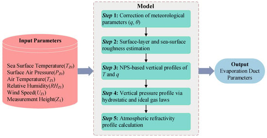
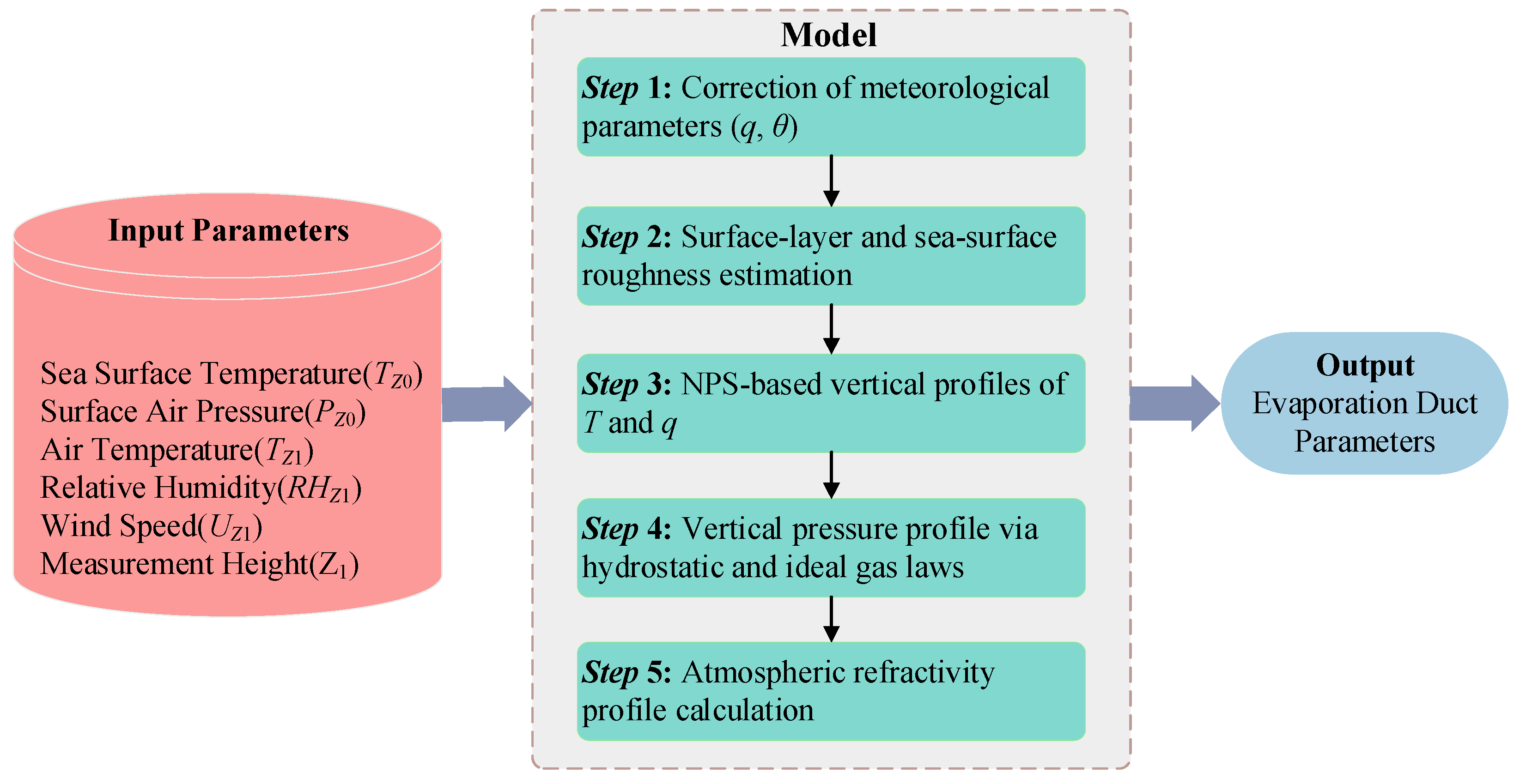
As illustrated in Figure 1, the NPS model follows a defined workflow to compute evaporation duct parameters. The vertical profiles of air temperature and specific humidity at height are given by:
where and denote the air temperature (K) and specific humidity (kg·kg−1) at height , respectively; and represent the sea surface temperature and specific humidity, respectively. , is the sea surface saturation-specific humidity calculated from the sea surface temperature. and are Monin–Obukhov characteristic scales (kg·kg−1) of potential temperature and specific humidity , respectively. is the von Kármán constant, typically taken as 0.4. denotes the temperature roughness height, is the universal temperature function, is the dry adiabatic lapse rate (≈0.00976 K·m−1), and is the Monin–Obukhov similar length.
Figure 1.
NPS model prediction flow chart.
The NPS model derives the evaporation duct pressure profile based on the vertical profiles of temperature, humidity, and air pressure:
where is the specific humidity, is the atmospheric pressure, and is the constant 0.62197.
By combining Equations (5)–(7), the modified refractivity profile derived from the NPS model is obtained. The corresponding NPS estimate of evaporation duct strength, , is then calculated as follows:
where is the pressure; is the air temperature; is the relative humidity; is the wind speed; is the height of the meteorological parameter; is the sea surface temperature. Here, the subscript “NPS” distinguishes the physical-model estimate from the dropsonde-derived EDS, which serves as the reference target for the CNRF model.
2.3. NPS Model Sensitivity Analysis
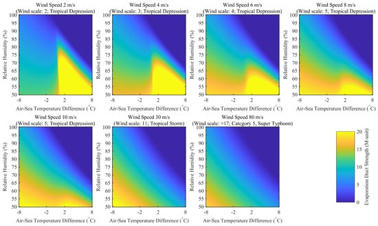
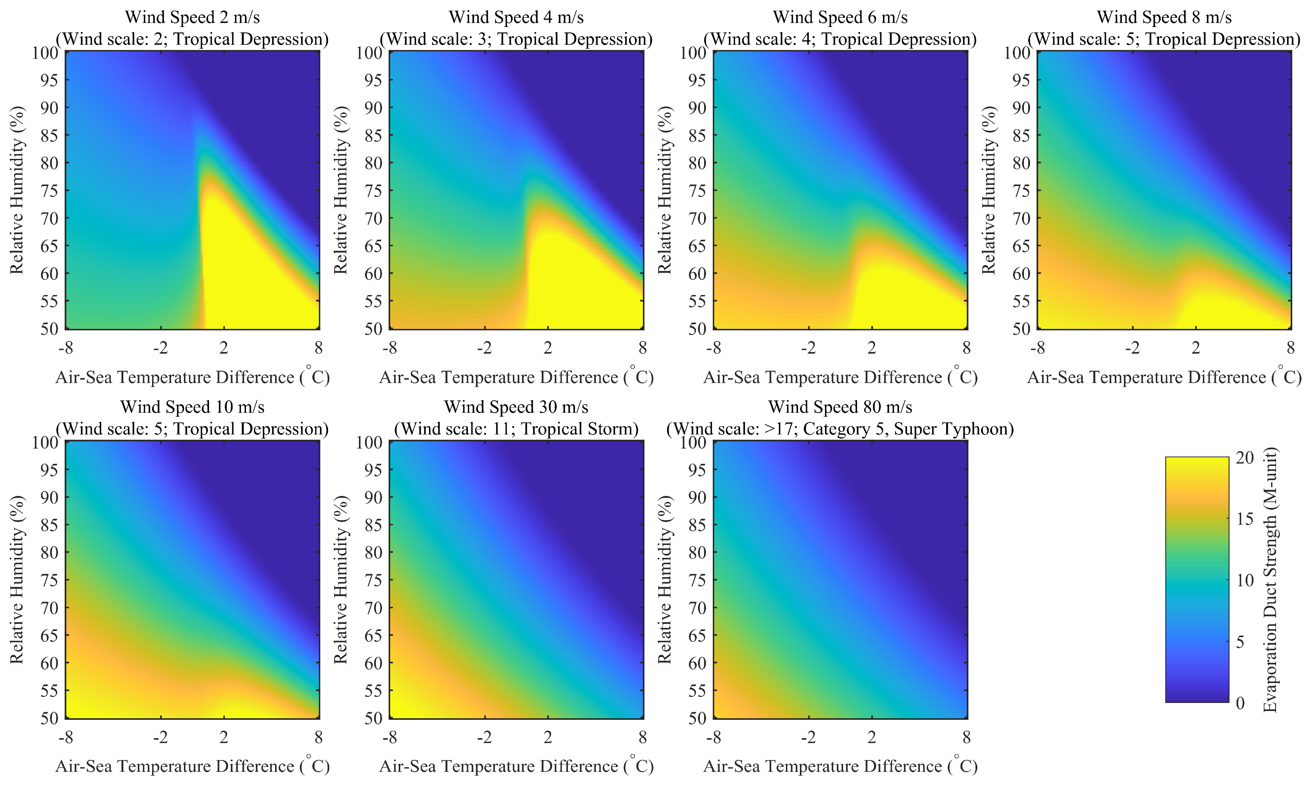
Figure 2 presents a controlled sensitivity experiment using the NPS model. In this experiment, sea-surface temperature and atmospheric pressure are fixed at 22 °C and 998.5 hPa, respectively. The air–sea temperature difference and relative humidity vary along the horizontal and vertical axes, while the panels represent different wind speeds ranging from 2 to 80 m·s−1. Across all wind-speed panels, generally decreases with increasing relative humidity at a fixed air–sea temperature difference. Higher ambient relative humidity reduces the moisture difference between the saturated sea surface and the overlying air, thereby weakening the vertical humidity gradient associated with evaporation-duct formation.
Figure 2.
Controlled NPS-model sensitivity of EDS to air-sea temperature difference and relative humidity at prescribed wind speeds of 2, 4, 6, 8, 10, 30, and 80 m·s−1. Sea-surface temperature and atmospheric pressure were fixed at 22 °C and 998.5 hPa, respectively. Relative humidity varied from 50% to 100%, and the air–sea temperature difference varied from −8 to 8 °C.
The influence of the air–sea temperature difference is nonlinear and varies with wind speed. Because is fixed in this experiment, variations along the horizontal axis reflect changes in air temperature relative to the constant sea-surface temperature. Local maxima in occur mainly under relatively low-humidity conditions at low-to-moderate wind speeds, whereas the maximum duct strength is generally reduced at wind speeds of 30 and 80 m·s−1. Therefore, Figure 2 indicates a consistently suppressive effect of increasing relative humidity within the tested parameter range, while the responses to air–sea temperature difference and wind speed are nonlinear.
The distinction between duct depth and refractive contrast also helps explain why EDH and EDS may respond differently to tropical-cyclone forcing. Previous research found that the low wind speed in the cyclone eye was associated with a reduced EDH [28]. Conversely, enhanced mechanical mixing may extend the duct layer vertically while weakening the modified-refractivity gradient, resulting in a deeper but weaker duct. Thus, both EDH and EDS are important because the maximum wavelength supported by an evaporation duct depends on the duct height and the change in modified refractivity across the duct [29].
3. Datasets and Methodology
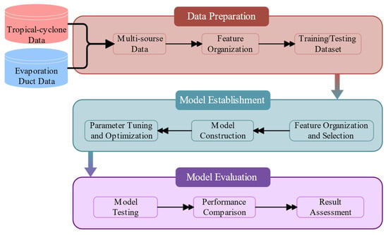
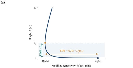
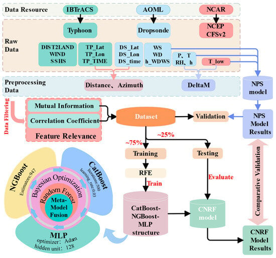
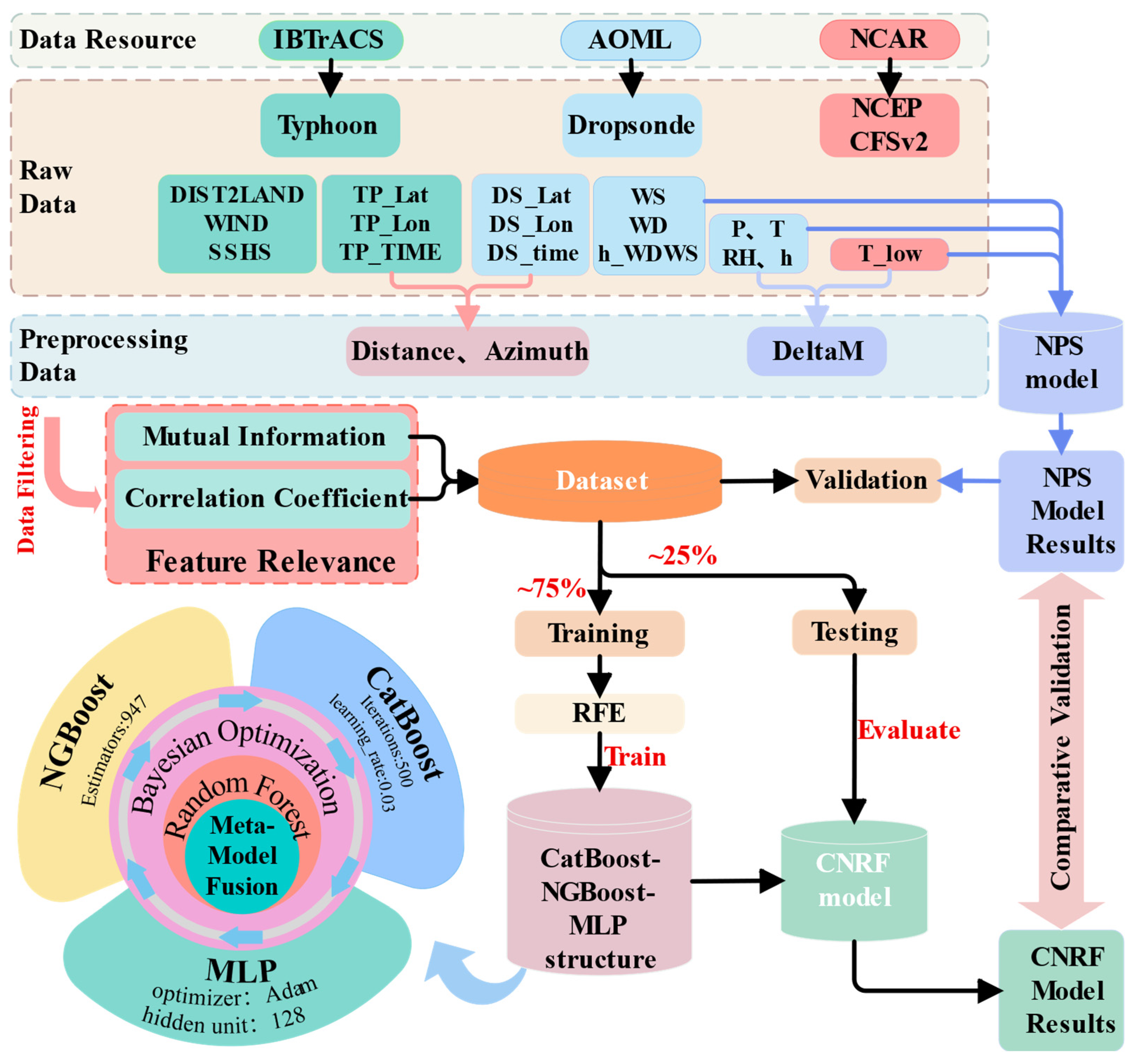
In the previous chapter, we conducted a qualitative analysis of the factors influencing evaporation duct formation and identified the relationships between wind speed and EDS. The study demonstrates that the strength of evaporation ducts in tropical cyclone-affected regions is closely related to tropical cyclone characteristics, and this relationship can be quantified through modeling. Building on this insight, this section establishes a multivariate estimation framework for EDS using tropical cyclone event observations from the Pacific and Atlantic Ocean regions. Figure 3 illustrates the basic structure of the proposed framework, encompassing critical steps such as data processing, model construction, and evaluation. The data-preparation module integrates the dropsonde-derived duct parameters with spatiotemporally collocated tropical-cyclone descriptors and constructs the event-level training and test sets. The model-establishment module includes feature selection, Bayesian hyperparameter optimization, base-learner training, and random-forest meta-learning. The model-evaluation module compares CNRF with the NPS baseline using held-out tropical-cyclone events and the independent Hurricane Fiona case. These steps collectively form a diagnostic regression framework for estimating contemporaneous EDS under tropical-cyclone conditions.
Figure 3.
Overall workflow of the proposed CNRF diagnostic regression framework.
3.1. Modeling Data
3.1.1. Evaporation Duct Datasets
The dropsonde profiles used to derive the reference EDS were obtained from the Atlantic Oceanographic and Meteorological Laboratory (AOML) of the National Oceanic and Atmospheric Administration (NOAA) and were collected during aircraft missions conducted by NOAA’s Hurricane Research Division (HRD) [30]. The measurements were primarily acquired through dropsonde deployments within tropical-cyclone environments. Dropsondes are typically released from several kilometers above sea level and record temperature, relative humidity, pressure, wind speed, wind direction, and Global Positioning System (GPS) position in real time throughout their descent.
The processed AOML dropsonde profiles have an approximately 5 m vertical resolution and extend from near the sea surface to altitudes of several kilometers. No additional vertical interpolation or resampling was applied to the observed atmospheric levels. For each profile, modified refractivity was calculated at the retained levels using quality-controlled pressure, temperature, relative humidity, and height, with the surface-endpoint treatment described below. The modified-refractivity values at the seven lowest valid levels within 0–40 m were fitted using:
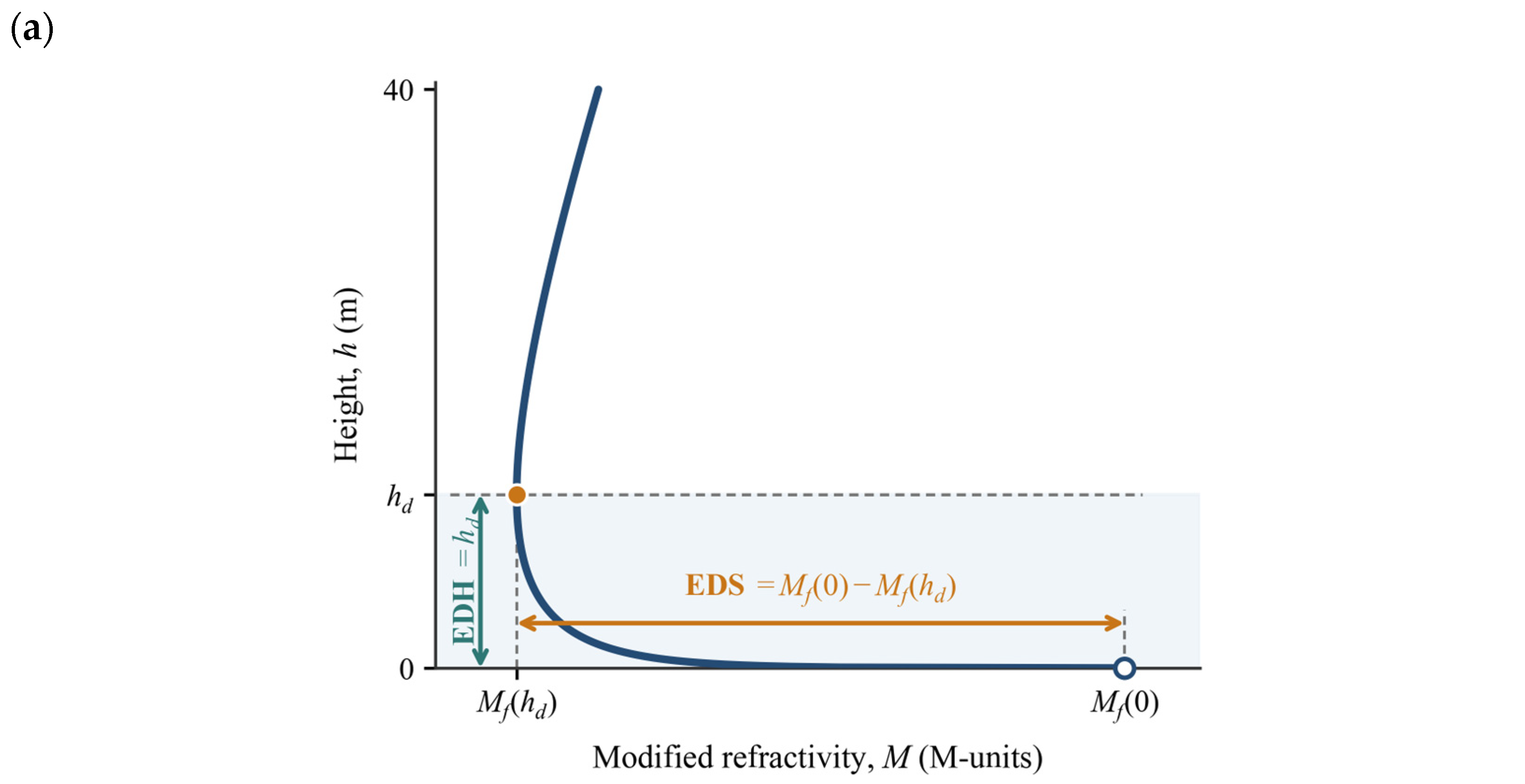
The EDH was identified as the local minimum of the fitted profile within this height range, where the gradient changed from negative to non-negative. EDS was then calculated as:
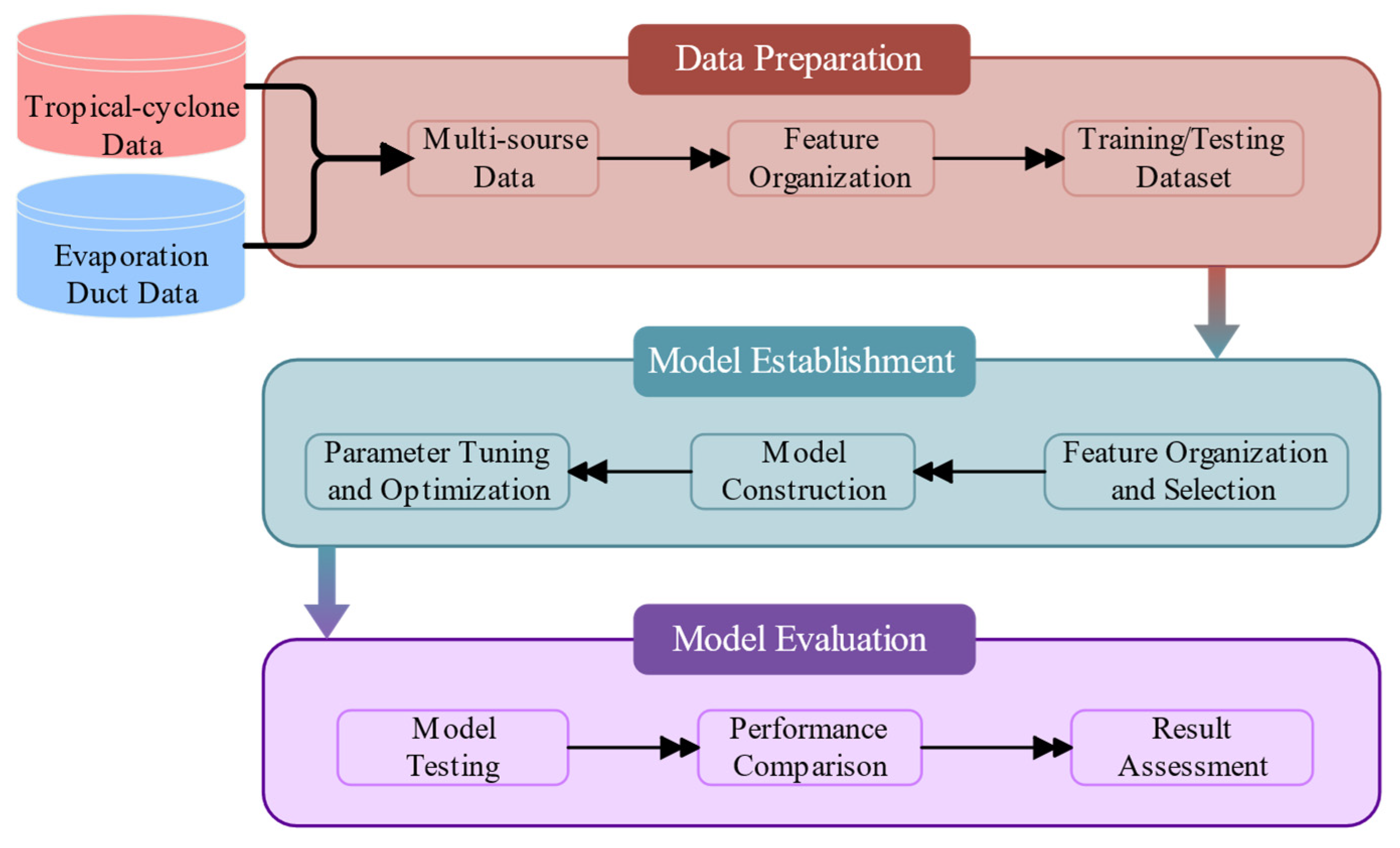
The definitions of EDH and EDS are illustrated schematically in Figure 4a. was used to identify the negative-gradient ducting layer, but it was not the sole criterion for determining the duct top. When no valid minimum was identified within 0–40 m, or when the derived duct height was zero, the profile was treated as non-ducting, and both EDH and EDS were assigned a value of zero.
Figure 4.
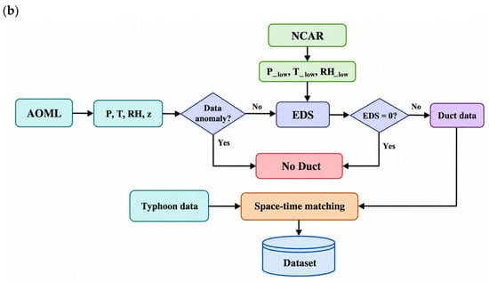
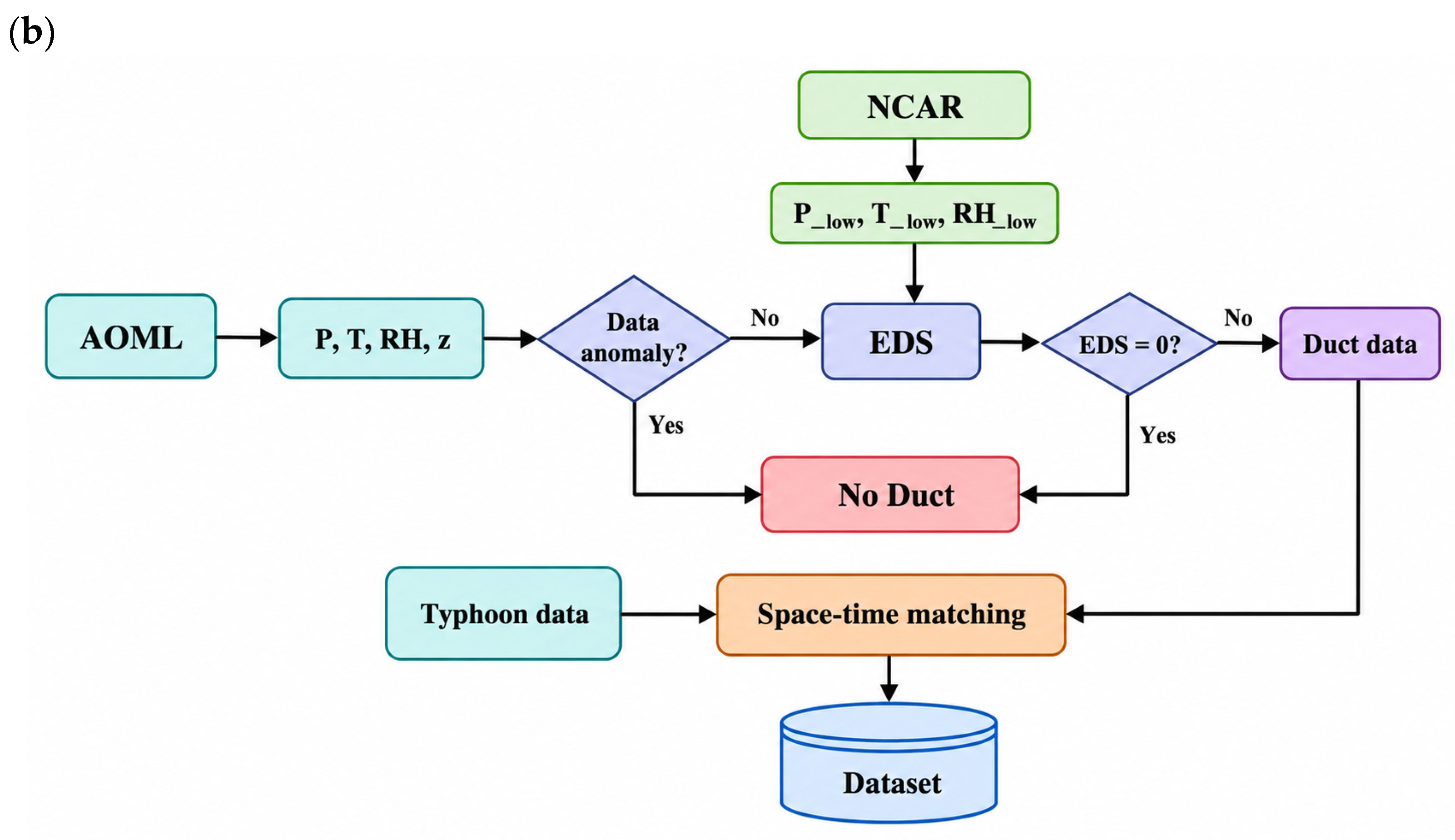
Diagnosis and processing of the dropsonde-derived reference EDS dataset. (a) Schematic of the fitted modified-refractivity profile showing EDH and EDS. (b) Workflow for constructing the dropsonde-derived reference EDS dataset.
After the initial quality-control procedure, the dataset comprised 4218 dropsonde profiles collected from 358 independent tropical-cyclone events. Following spatiotemporal collocation and restriction to observations within 500 km of the corresponding storm centers, 1425 profiles with valid duct diagnoses were obtained. Among these profiles, 1347 were identified as ducting cases and 78 as non-ducting cases, corresponding to proportions of 94.5% and 5.5%, respectively. The non-ducting cases, for which both EDH and EDS were assigned a value of zero, were retained when calculating the duct-occurrence proportion but were excluded before constructing the final EDS regression dataset. The final regression dataset therefore comprised 1347 ducting profiles from 142 independent tropical-cyclone events. Among these, 31 profiles from Fiona were reserved exclusively for independent case validation, while the remaining 1316 profiles from 141 tropical-cyclone events were used for model development and evaluation. The complete data-processing workflow is summarized in Figure 4b, with the main steps as follows:
- For each dropsonde profile, measurements below 40 m were screened for missing or physically implausible values. A profile was retained only when pressure, temperature, relative humidity, and height were simultaneously available at a minimum of seven valid vertical levels within 0–40 m. Profiles containing fewer than seven complete valid levels were excluded from the subsequent EDS calculation. Missing values within the dropsonde profiles were neither imputed nor vertically interpolated. In addition, a profile was retained only when its lowest valid observation was located within 7 m of the sea surface. This requirement ensured that the observed profile extended sufficiently close to the surface to construct the 0–40 m modified-refractivity profile.
- Although dropsondes continuously measure atmospheric variables throughout their descent, the terminal measurements close to splashdown may be unavailable or may deviate from the representative ambient near-surface conditions, particularly under severe tropical-cyclone environments. To provide a consistent surface boundary for the modified-refractivity-profile fitting, surface temperature was obtained from the National Centers for Environmental Prediction (NCEP) Climate Forecast System Version 2 (CFSv2) Selected Hourly Time-Series Products (the surface-temperature variable, tmpsfc), archived at U.S. National Science Foundation (NSF) National Center for Atmospheric Research (NCAR) Geoscience Data Exchange (GDEX) as dataset D094001 [31]. For each dropsonde profile, the CFSv2 field corresponding to the recorded Coordinated Universal Time (UTC) day and hour was selected, and the values at the four surrounding grid cells were bilinearly interpolated to the dropsonde splash-point latitude and longitude; no temporal interpolation was applied. At the surface endpoint, temperature was replaced by the collocated CFSv2 surface temperature, relative humidity was set to 98%, and pressure was retained from the corresponding dropsonde record. The remaining vertical levels retained the original quality-controlled dropsonde measurements. This procedure was used to supplement the surface boundary rather than to replace the complete dropsonde profile.
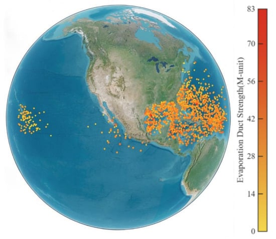
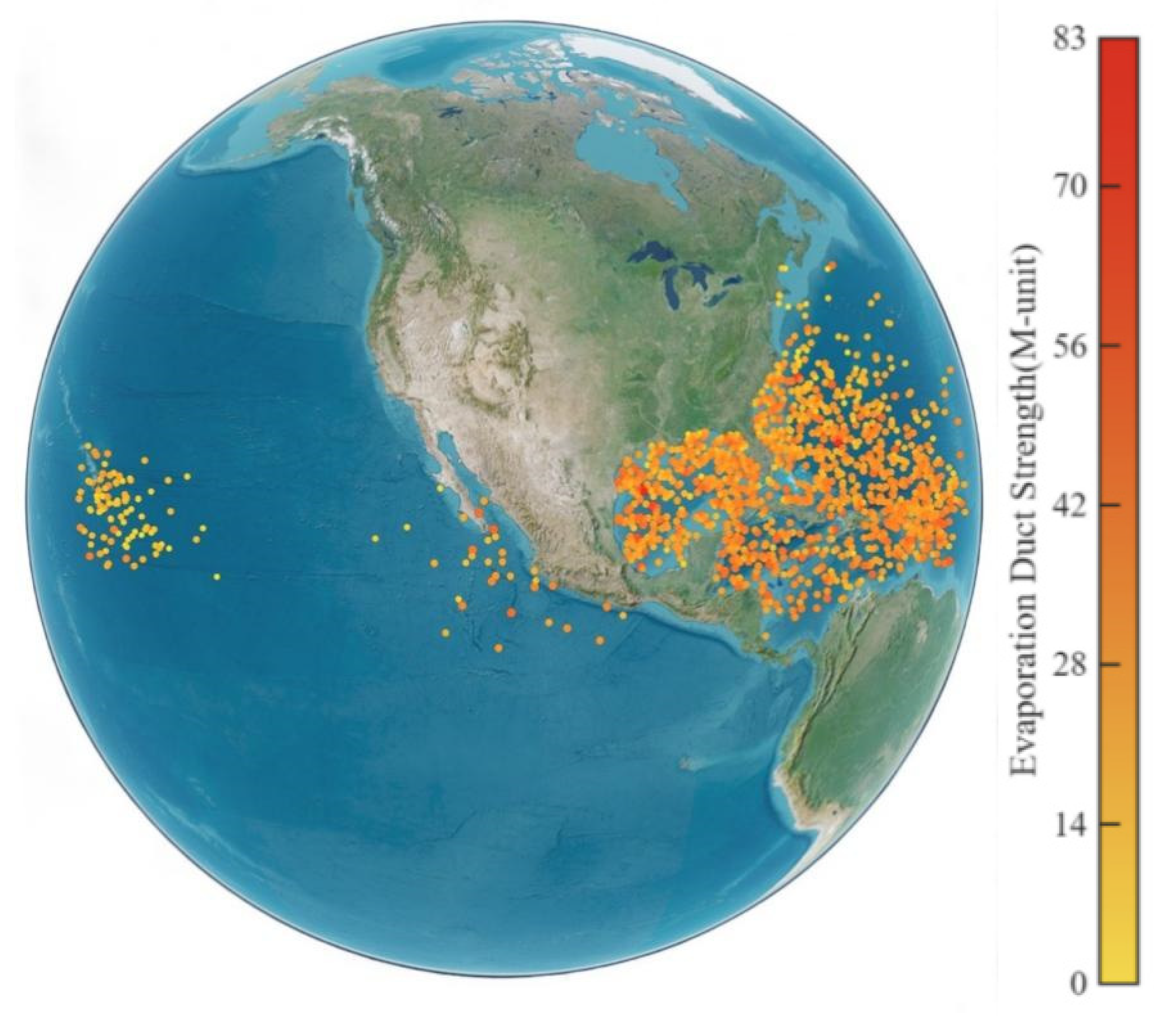
- Each dropsonde yields one set of evaporation duct parameters; a zero duct height is treated as the absence of ducting. After outlier removal, the duct estimates are collocated with tropical cyclone data in both time and space to construct the final dataset. The resulting duct fields are shown in Figure 5, where color indicates the dropsonde-derived EDS.Figure 5. Spatial distribution of EDS derived from dropsonde observations.
- The EDS used to train and evaluate the CNRF model was derived from the quality-controlled dropsonde profiles supplemented with near-surface meteorological information. Throughout this study, EDS without a model subscript denotes this dropsonde-derived reference value. In contrast, is independently calculated using the NPS model based on Monin–Obukhov similarity theory and bulk air–sea parameterization. Although the two calculations use the same modified-refractivity equation and EDS definition for comparability, is not used to construct the CNRF training target.
3.1.2. Tropical Cyclone Datasets
Tropical cyclone records are obtained from IBTrACS [22,23], which is developed and maintained by NOAA’s National Centers for Environmental Information (NCEI) [32]. The archive consolidates best-track information for tropical cyclones across the Pacific, Atlantic, and Indian Oceans. IBTrACS provides storm name, timestamp, center latitude and longitude, intensity class, translation speed, and motion direction; for a subset of events, central pressure and the radius of 34-kt winds (R34) are also available.
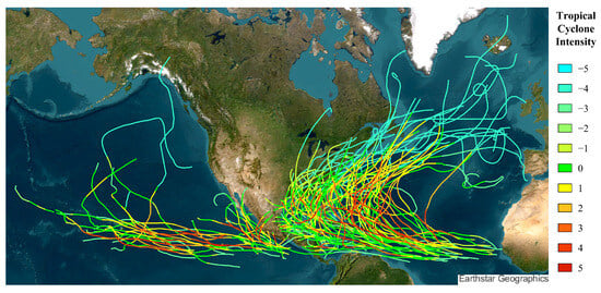
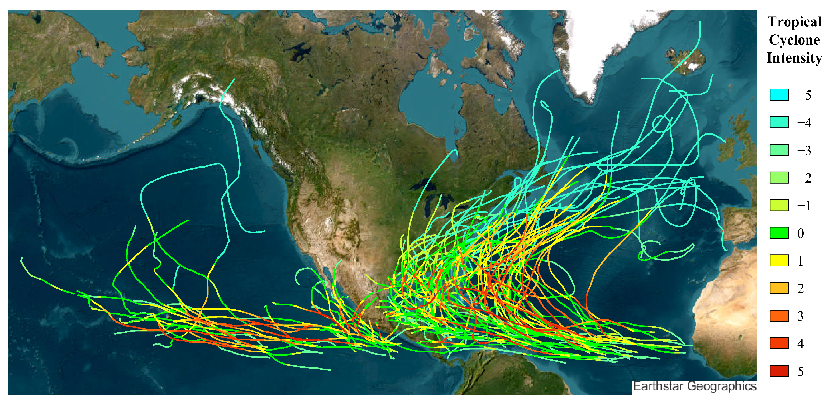
The compiled cases span nearly three decades and primarily cover storms over the North Atlantic and the Northeast Pacific. Figure 6 maps all IBTrACS tracks used in this study. The U.S.-agency Saffir–Simpson Hurricane Scale classification (IBTrACS field USA_SSHS) classes are −5 (unknown), −4 (post-tropical), −3 (miscellaneous disturbance), −2 (subtropical), −1 (tropical depression), 0 (tropical storm), and 1–5 (Categories 1–5 hurricanes). Track color encodes the IBTrACS intensity class, with 11 categories in total: red indicates the highest class, and colors shift gradually toward cyan as intensity decreases.
Figure 6.
Tracks of the tropical-cyclone events used in this study. Track color represents the IBTrACS USA_SSHS class, ranging from −5 to 5.
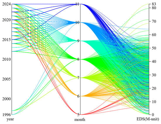
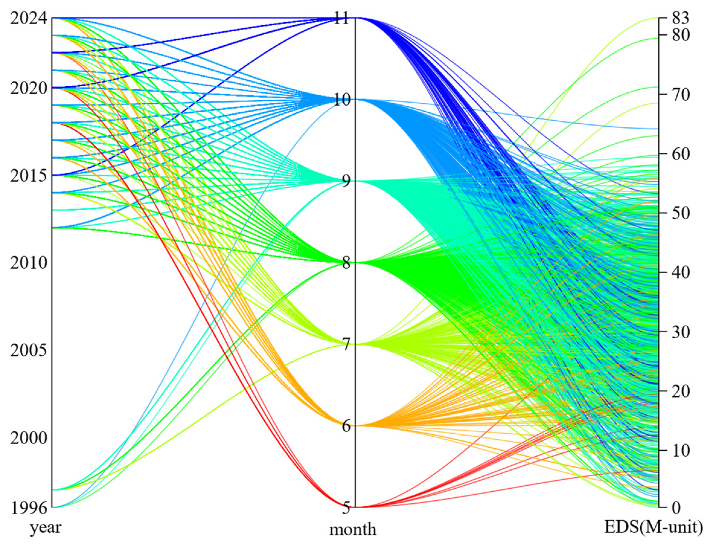
Figure 7 presents the temporal distribution of EDS using a parallel-coordinate plot. Each line represents one valid profile and connects its observation year, month, and duct strength on the three respective axes, which use independent numerical scales. The observations are mainly distributed from May to November, with a concentration between August and October, reflecting both the seasonal occurrence of tropical cyclones and the availability of dropsonde observations. The gap during 1998–2011 is attributable to the unavailability or insufficient number of storm observations. Therefore, the temporal distribution should be interpreted with consideration of the uneven data coverage. Because the training and test sets were divided by tropical-cyclone event identifier (typh_SID) rather than by year, this temporal gap did not directly determine the data partition.
Figure 7.
Parallel-coordinate representation of the temporal distribution of EDS. Each polyline represents one valid dropsonde profile and connects its observation year, observation month, and EDS. Line color indicates the observation month.
3.1.3. Data Optimization
Initial feature relevance was evaluated using both correlation and mutual information with EDS. As shown in Figure 8, the sector radius represents the signed correlation coefficient, whereas the angular width represents mutual information, with a larger width indicating stronger dependence. The prefixes DS and TP denote dropsonde-derived and tropical-cyclone-related variables, respectively. Among the dropsonde-derived variables, lower-level temperature (DS_T_low) shows a relatively strong positive association with duct strength, whereas relative humidity at the penultimate valid level (DS_RH_Penul) exhibits a pronounced negative association. These relationships are physically reasonable because lower-level temperature affects surface evaporation and the near-surface modified-refractivity gradient, while higher relative humidity at the penultimate level may reduce the vertical moisture gradient associated with evaporation-duct formation. DS_P_Penul and storm-relative variables such as distance and azimuth also show appreciable dependence, indicating that duct strength is jointly influenced by lower-atmospheric thermodynamic conditions and the observation position relative to the storm.
Correlation and mutual information were used as complementary preliminary diagnostics: correlation describes primarily linear relationships, whereas mutual information can capture nonlinear dependence. These statistics did not directly determine the final feature subset; instead, they provided an initial assessment of feature relevance before recursive feature elimination (RFE) was applied to the training data to remove redundant or weakly contributing variables.
Figure 8.
Correlation and mutual information analyses between the candidate variables and EDS. The definitions and units of all variables are provided in Table 1; the prefixes DS and TP denote dropsonde-derived and tropical-cyclone-related variables, respectively.
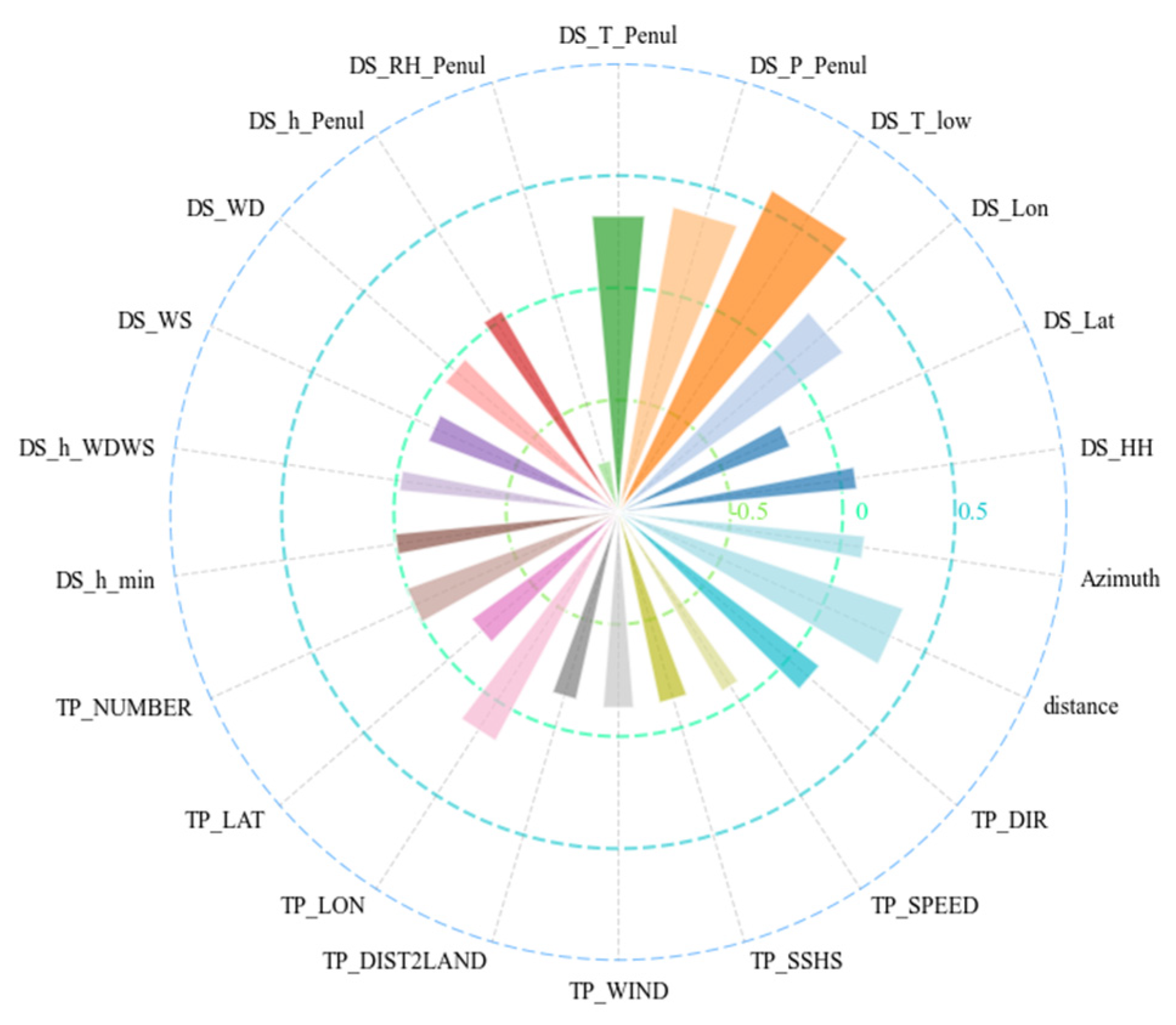
Table 1.
Definitions of the candidate variables used in Figure 8.
3.1.4. Data Correlation Analysis
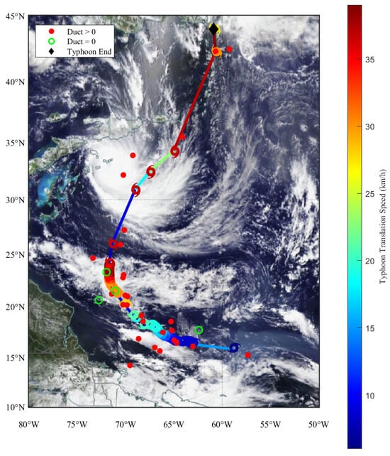
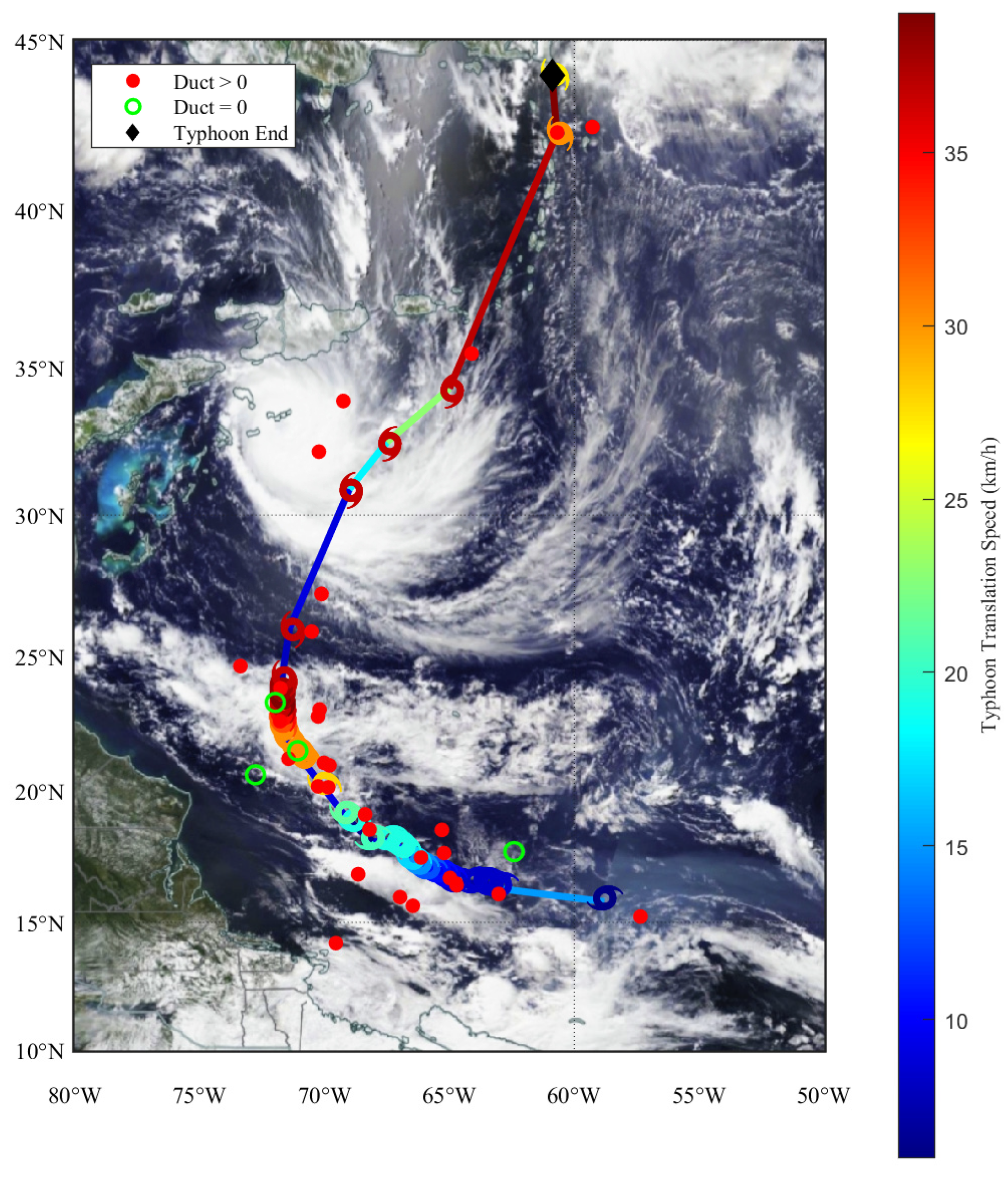
To further illustrate the association between evaporation duct characteristics and tropical-cyclone conditions, Fiona (2022), which was completely excluded from model development, is examined as an independent representative case. The storm track and collocated duct observations are shown in Figure 9. Fiona developed over the central Atlantic to the northeast of South America, initially moved westward, and then recurved northward, making landfall on the evening of 18 September. The maximum distance from the mainland is approximately 900 km, while most samples were collected when the storm was within 300 km of land.
Figure 9.
Distribution of dropsonde observations around Hurricane Fiona (2022).
In Figure 9, red markers denote ducting, and green circles indicate non-ducting conditions based on dropsonde-derived estimates. During Fiona, ducting occurred in 88.6% of the collocated samples. Track color transitions from blue to red as translation speed increases (color bar on the right), reaching a maximum of 39 kt (1 kt = 1 nautical mile per hour). Storm symbols indicate the direction of motion, with azimuth defined clockwise from true north. Symbol color encodes central wind speed (blue–red gradient), with a maximum of 120 kt; a black diamond marks the storm endpoint.
Duct evolution exhibits clear stage dependence. In the early stage, duct formation may be favored when a moist sea surface is overlain by relatively drier air, producing a pronounced vertical moisture gradient. As the storm intensifies, central winds strengthen, and central pressure decreases, making ducting less favorable near the core. Ducts occur more readily at larger radii from the center, where strength is often higher. In the late stage, weakening winds are accompanied by a renewed tendency for duct formation; although duct strength is lower, the duct structure appears comparatively more stable.
3.2. Modeling Method
To analyze tropical cyclone-driven perturbations in evaporation duct parameters, tropical cyclone descriptors are incorporated as additional inputs to represent their linkage to EDS. This design leverages storm information more effectively and enhances cross-dataset adaptability. The framework adopts a stacked ensemble with CatBoost, NGBoost, and an MLP as base learners, and a random forest as the meta-learner. In the second stage, the meta-learner takes base-model predictions as inputs and learns a data-driven combination of their outputs. By integrating learners with different modeling characteristics, the ensemble reduces dependence on any single model and provides a flexible strategy for EDS prediction under highly variable tropical cyclone conditions. Accordingly, the present task is formulated as conditional EDS regression for profiles in which an evaporation duct has already been diagnosed. CNRF does not estimate the probability of duct occurrence, and all reported regression metrics refer only to the ducting subset.
Each component provides a different learning mechanism. CatBoost is well-suited to nonlinear tabular regression and can capture interactions between storm descriptors and meteorological measurements. NGBoost was included as a distributional boosting learner whose natural-gradient optimization and distribution-based loss provide a modeling mechanism complementary to CatBoost and MLP. In the present CNRF implementation, however, only the conditional mean predicted by NGBoost was supplied to the Random Forest meta-learner. The MLP provides smooth function approximation that complements the piecewise predictions of the tree-based models. The Random Forest meta-learner subsequently combines the point predictions generated by the three base learners.
3.2.1. CatBoost
CatBoost is a gradient-boosting method designed to handle datasets containing categorical features [33]. It is built on symmetric decision trees, where the same rule splits all leaves at the same depth. At each boosting step, candidate splits are evaluated, and the feature–threshold pair that minimizes the loss is selected, after which the split is applied across all nodes at that depth. Performance is improved iteratively by fitting residuals from the previous stage. In addition, CatBoost employs target-statistics encoding for categorical variables, which helps reduce overfitting and alleviates prediction shift and gradient bias, thereby improving accuracy and generalization.
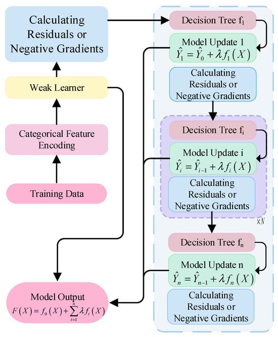
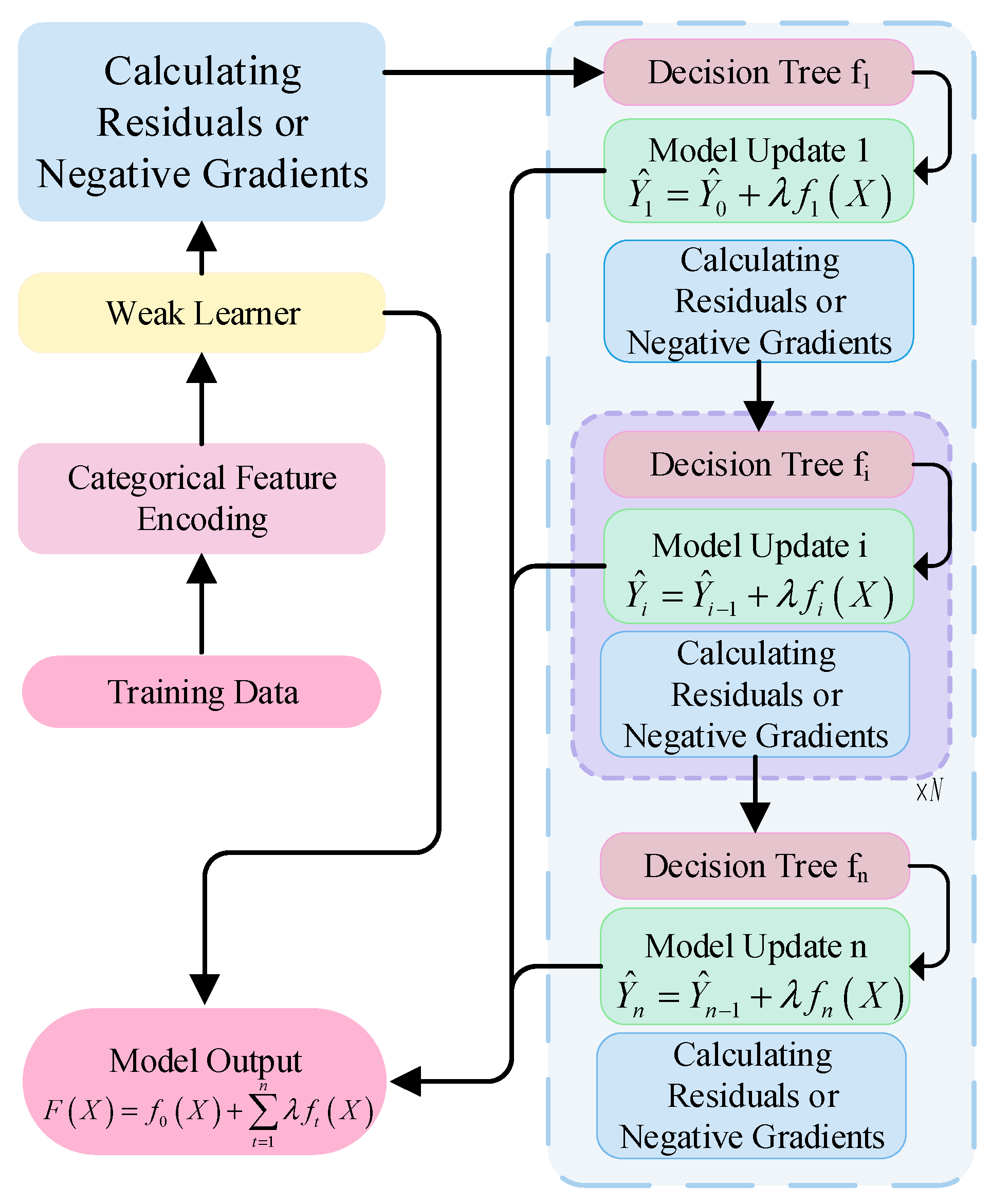
Figure 10 illustrates the CatBoost workflow. During tree construction, candidate splits are assessed by enumerating feature–threshold combinations at each node, including feature selection, threshold determination, and symmetric splitting. Feature selection quantifies the contribution of each variable to the target, whereas symmetric splitting enforces the tree’s constrained structure by using the same selected feature and threshold for all nodes at a given depth.
Figure 10.
Schematic diagram of CatBoost model.
The training starts from an initial weak learner, denoted as , with predictions . In the regression task, the difference between the observed value and the current model prediction is computed, followed by the evaluation of the negative gradient of the loss function with respect to the prediction, where denotes the iteration index:
Using the residual and negative gradient as the new target values, a symmetric decision tree is constructed. According to the newly trained decision tree, the formula is used, where denotes the learning rate, which controls the contribution of each tree in the model. By repeating the above process and iterative training until the preset stop conditions are met, the final prediction function is:
3.2.2. NGBoost
EDS varies nonlinearly under tropical-cyclone conditions and is influenced by multiple meteorological drivers. NGBoost was included as a probabilistic boosting algorithm that models the conditional distribution of the response variable and optimizes the distribution parameters using natural gradients [34]. Unlike conventional gradient boosting, which directly estimates a point response, NGBoost learns the parameters of a prespecified conditional distribution using a proper scoring rule. This distribution-based training mechanism provides a complementary inductive bias within the heterogeneous ensemble. In the present study, the conditional mean predicted by NGBoost was extracted as its base-model output. The predictive scale and prediction intervals were not propagated to the Random Forest meta-learner; therefore, the final CNRF was evaluated as a point-regression model.
NGBoost predicts the conditional probability distribution of the output variable given the input variable . The prediction distribution of the model is represented by a set of parameters in the form of:
The negative log-likelihood scoring rule was used to evaluate the agreement between the predicted conditional distribution and the observed response:
NGBoost uses the Fisher information matrix to rescale the conventional gradient according to the local geometry of the statistical parameter space. The Fisher information matrix is defined as:
The natural gradient is the projection of the standard gradient in the statistical parameter space. It will be used as the residual target to train the base learner to fit the update direction of each distribution parameter, expressed as:
NGBoost adopts a forward phased upgrade strategy. At round , a regression model is trained for each distribution parameter to fit the direction of the corresponding natural gradient, and the model parameter is updated to:
where is the learning rate. After multiple iterations, NGBoost outputs the parameters of the conditional predictive distribution. In the present CNRF implementation, the conditional mean, , was extracted as the NGBoost point prediction, whereas the predictive scale parameter was not used in the subsequent fusion stage.
3.2.3. MLP
Tree-based models may struggle to represent smooth trends. Multivariate regression, however, often requires high-dimensional interactions. An MLP is therefore employed to provide smooth function approximation and improve local continuity in the feature space [35].
An MLP is a general-purpose approximator composed of stacked neuron layers. It is widely used for classification and regression. Information propagates forward from the input layer through hidden layers to the output layer. Gradients are computed by backpropagation. An optimizer then updates the weights and biases. Nonlinear transformations arise from weighted sums followed by activation functions in the hidden layers. In this way, the MLP can approximate nonlinear mappings. The number of output-layer units matches the output dimension.
3.2.4. CNRF Model Construction
Estimating EDS under tropical-cyclone conditions is formulated as a contemporaneous diagnostic regression task. All input variables and the reference EDS are collocated at the same observation time; therefore, the CNRF model estimates EDS for previously unseen profiles or tropical-cyclone events but does not forecast EDS at a future lead time. The purpose is to establish the relationship between tropical cyclone meteorological parameters and duct strength. This mapping is highly nonlinear, and the input variables originate from multiple agencies with heterogeneous standards. In addition, tropical cyclone environments exhibit strong variability. To better exploit tropical cyclone descriptors, a stacking ensemble is adopted. Base-model predictions from the three learners are used as inputs to a higher-level meta-model. This yields the CNRF model. The overall workflow is shown in Figure 11 and consists of three stages:
Figure 11.
Overall flow chart.
- Model construction: The input variables are normalized to place tropical cyclone descriptors and dropsonde measurements on a common scale. To avoid sample leakage among highly correlated observations from the same tropical cyclone, the non-Fiona samples are split at the event level according to typh_SID. Thus, all samples from one tropical cyclone are assigned only to the training set or the test set, with an approximate training proportion of 75%. RFE is then applied on the training set to remove redundant features. The input feature vector is defined as:where denotes the selected height-dependent meteorological features derived from dropsonde measurements, denotes the tropical cyclone-related features, and denotes the azimuth from the tropical-cyclone center to the dropsonde location. The height coordinate is not separately included, since the vertical information is already embedded in these meteorological features. The complete 0–40 m dropsonde profile, fitted modified-refractivity profile, EDH, and reference EDS were not included as model inputs.
- Hyperparameter optimization and training: Automatic hyperparameter tuning is performed using Bayesian optimization. The optimal configuration uses 500 iterations and a learning rate of 0.03 for CatBoost; NGBoost adopts 947 estimators; and the MLP is trained with Adam and 128 hidden units. These settings define the final model configuration used in the following experiments. A random-forest meta-model is then used to combine the outputs of the base learners. CatBoost, NGBoost, and MLP represent different nonlinear learning mechanisms and exhibit different error characteristics under varying tropical-cyclone conditions. A linear or ridge-regression combiner would assign globally fixed weights to their outputs, whereas the random-forest meta-learner can represent nonlinear relationships among the out-of-fold predictions of the base learners. This enables the fusion stage to indirectly adjust to regime-dependent differences in tropical-cyclone intensity, wind speed, and coastal distance. The random-forest meta-learner was therefore introduced primarily to balance the complementary error characteristics of the three learners. At the meta-learning stage, five-fold out-of-fold training was applied. In each fold, the random-forest meta-learner was fitted using the base-model outputs from the other four folds and generated predictions for the held-out fold, while the final test predictions were averaged across the fold-specific meta-models. The event-level test set was not involved in either base-learner or meta-learner training. Given input , the model predicts EDS as:where are the outputs of the individual sub-models, denotes the output of the meta-model, denotes the output of the CNRF meta-model.The computational cost of the CNRF mainly comes from the three base learners and the Random Forest fusion stage. For the MLP component, seven features are retained after RFE, and the network structure is 8–128–64–1, corresponding to approximately 1.87 × 10⁴ floating-point operations (FLOPs) for single-sample inference. For the tree-based components, including CatBoost, NGBoost, and Random Forest, the inference cost is mainly related to the number of trees and tree depth. Therefore, the overall computational cost of CNRF is higher than that of a standalone learner because multiple base models must be evaluated before fusion. Although the complete CNRF requires more computation than an individual learner, model training is performed offline on a relatively modest dataset. During inference, the three trained base learners first generate their estimates, and the trained random-forest meta-learner then performs the final fusion. This additional step did not constitute a practical computational bottleneck in the present experiments, and predictions could be obtained immediately after the base-model outputs were generated. Therefore, the additional computational cost was considered acceptable given the reduced central bias and more balanced predictive behavior.
- Evaluation: Model performance is evaluated using the dropsonde-derived EDS as the common reference. The reference EDS and use the same modified-refractivity equation and EDS definition but are not obtained under the same profile-construction assumptions. As described in Section 3.1.1, the reference EDS is diagnosed from the observed multilevel dropsonde profile, whereas is calculated independently from the bulk meteorological inputs in Equation (8) using the Monin–Obukhov-similarity-based profile reconstruction. and are independently compared with the same reference EDS on the event-level held-out test set.
4. Results and Discussion
Four metrics, including root mean square error (RMSE), mean absolute error (MAE), coefficient of determination (), and improvement rate () are employed to evaluate the estimation accuracy and robustness of the CNRF model. In the following evaluation metrics, denotes the dropsonde-derived reference EDS, whereas and denote the corresponding CNRF and NPS estimates, respectively.
- RMSE: The square root of the mean squared difference between the predicted value and the reference value is used to quantify the overall magnitude of prediction errors. A lower RMSE indicates better model performance:where n is the number of samples.
- MAE: The average absolute difference between the predicted value and the reference value is evaluated to reflect the overall magnitude of the prediction error without considering its direction. A lower mean absolute error indicates better model performance:where n is the number of samples.
- : The coefficient of determination quantifies the proportion of variance in the reference values explained by the model relative to a mean-value baseline. A value closer to 1 indicates better agreement between the estimates and reference values:
- : evaluate the improvement percentage of the prediction results of the model based on the CNRF model method relative to the numerical inversion model. In this section, the NPS model is selected for comparison, where is the prediction error of the NPS model, and is the prediction error of the evaporation duct characteristic parameter analysis model proposed in this paper:
4.1. Comparative Analysis
AOML dropsonde observations and tropical cyclone case data from 1996 to 2024 are compiled and analyzed in this study. The complete record of Hurricane Fiona is reserved for validation, while all remaining cases are split into training and test sets. Evaluation metrics are defined in Equations (20)–(24).
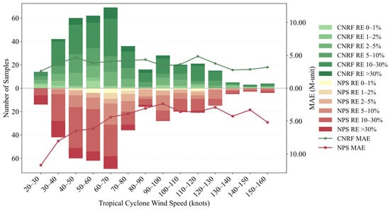
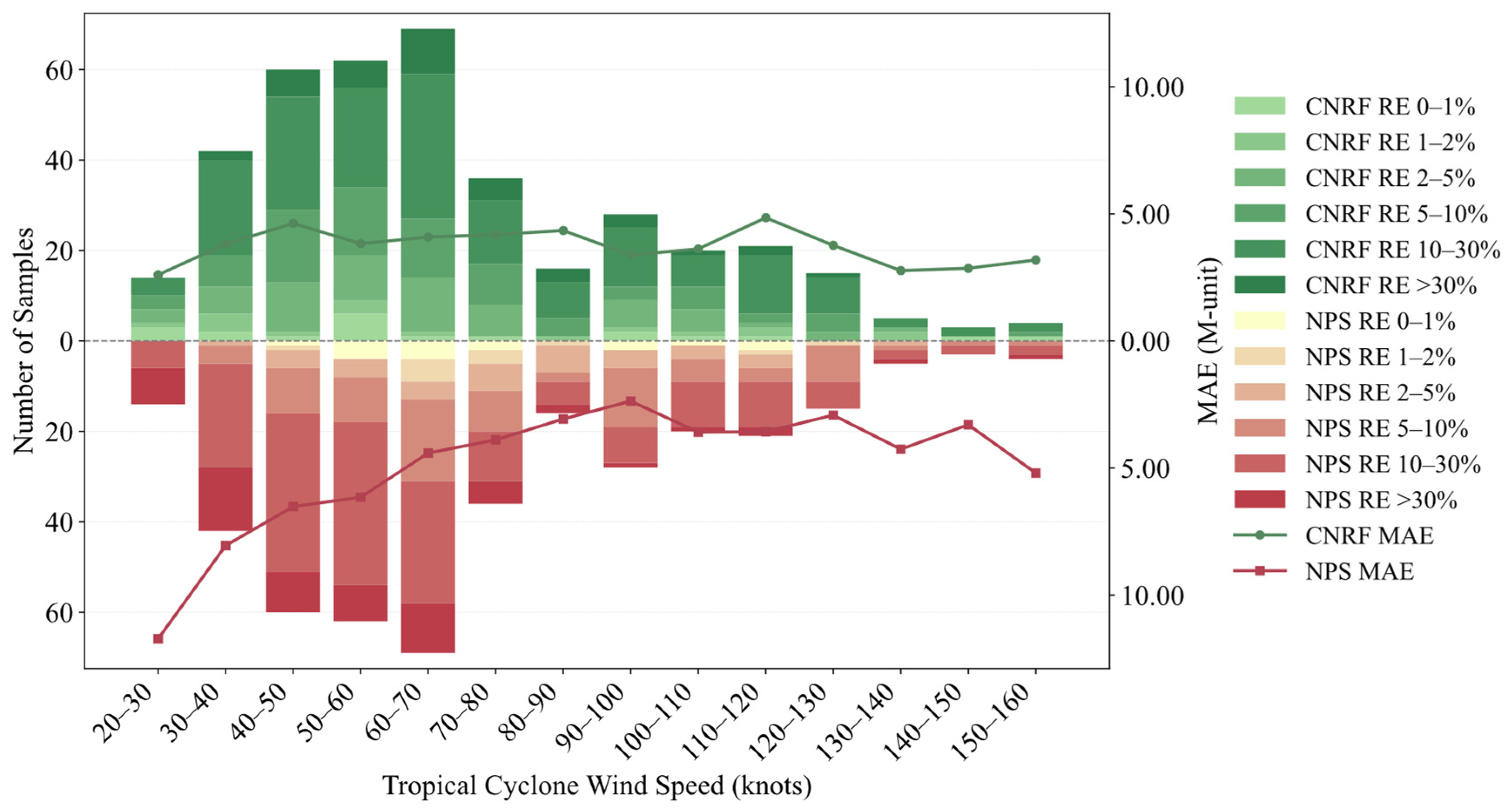
As shown in Figure 12, wind speeds in the dataset mainly range from 20 to 130 knots, with 63.8% of the samples falling within the 30–80-knot interval. Using the constructed duct-strength dataset, the performance of the CNRF model is evaluated against that of the NPS numerical model. The NPS model achieves an MAE below 5 M-unit in only a limited number of wind-speed bins, and its maximum bin-wise MAE exceeds 10 M-unit in the 40–60-knot range. In contrast, the CNRF model maintains a consistently lower MAE, which generally remains around or below 5 M-unit across the wind-speed bins. The stacked bars represent the number of samples in different absolute-relative-error intervals. Lighter shades correspond to smaller relative-error intervals, whereas darker shades indicate larger relative errors. Moreover, the proportion of samples with absolute relative errors below 30% increases from approximately 84% for the NPS model to 90.13% for the CNRF model.
Figure 12.
Wind-speed-binned error statistics for the CNRF and NPS models on the test set. The green and red stacked bars show the numbers of CNRF and NPS samples, respectively, within different absolute-relative-error (RE) intervals. The solid lines show the bin-wise MAE (M-unit) of the two models.
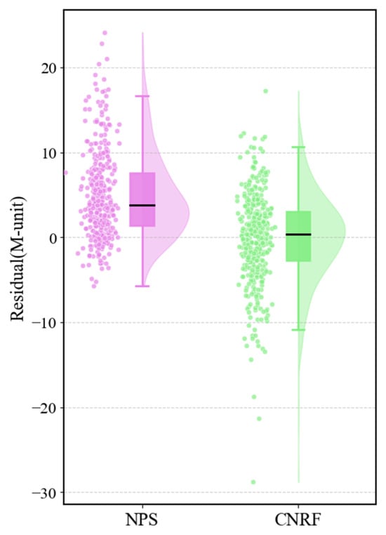
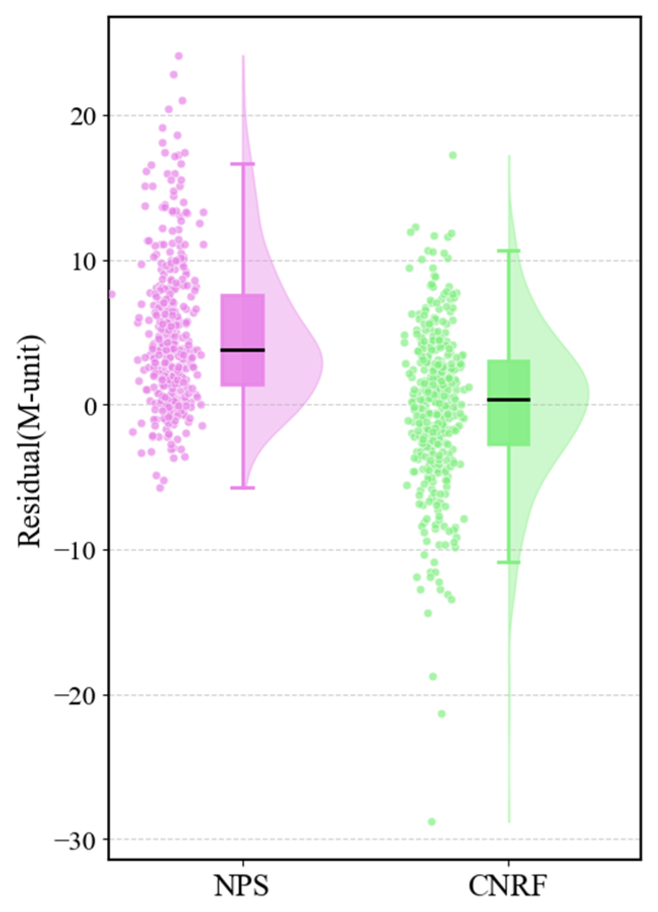
To further probe the error structure, this study visualizes all test-set points using a raincloud plot and compares the residual distributions of the CNRF model and the NPS model. Figure 13 shows that CNRF residuals are more concentrated around zero and more nearly normally distributed. In contrast, the NPS model exhibits a substantially higher median residual (3.792 M-unit) than the CNRF model (0.397 M-unit). Furthermore, the NPS model demonstrates a broader interquartile range of 6.224 M-unit compared with 5.723 M-unit for CNRF. Collectively, these metrics underscore the capacity of the CNRF model to effectively mitigate both systematic bias and error dispersion relative to the NPS baseline. Although both CNRF and NPS use contemporaneous observational meteorological information, they employ different input structures and modeling assumptions. NPS reconstructs the near-surface atmospheric profile from bulk air–sea variables using similarity theory, whereas CNRF estimates EDS from selected near-surface meteorological variables and tropical-cyclone descriptors. Accordingly, NPS is used as an established physical-model benchmark, and the comparison is interpreted with consideration of these differences in input information and model formulation.
Figure 13.
Residual distributions of EDS (CNRF model vs. NPS model).
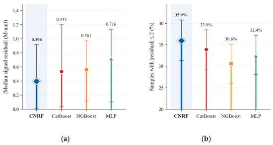
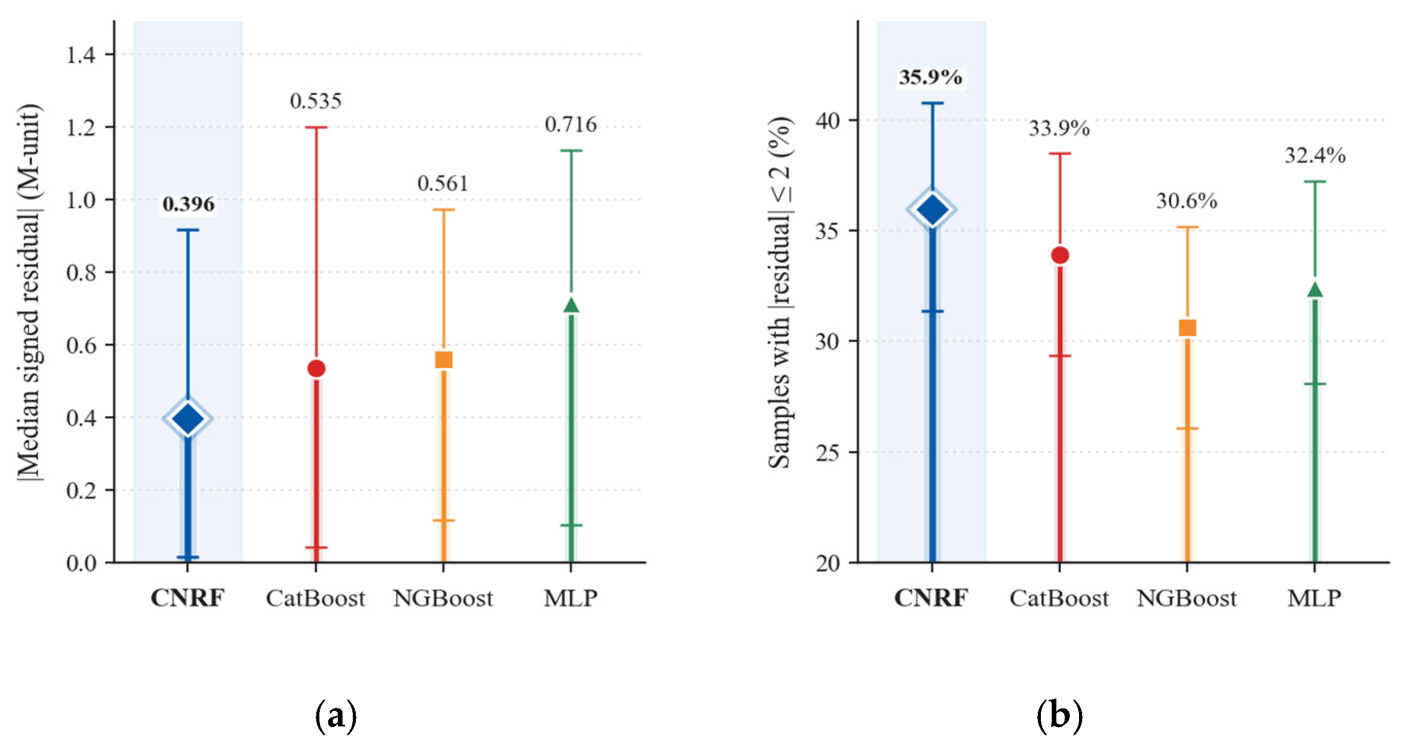
Figure 14 compares the central residual characteristics of CNRF with those of the individual CatBoost, NGBoost, and MLP learners. CNRF produces the smallest absolute median signed residual (0.396 M-unit) and the highest proportion of samples with an absolute residual not exceeding 2 M-unit (35.9%). However, the individual learners achieve lower RMSE and MAE and higher values than the complete CNRF model, with MLP obtaining the best aggregate performance. This contrast indicates that the random-forest fusion stage reduces central prediction bias and increases the proportion of samples with closely estimated values, whereas the individual learners maintain better overall error performance. Overall, CNRF provides improved residual balance at the cost of slightly larger aggregate errors.
Figure 14.
Residual-based comparison of CNRF and the three individual base learners on the held-out test set. (a) Absolute value of the median signed residual, . (b) Percentage of samples with an absolute residual not exceeding 2 M-unit. Markers denote point estimates, and error bars represent 95% confidence intervals obtained from 5000 bootstrap resamples.
Previous data-driven studies have applied deep learning to range-dependent evaporation-duct inversion [15] and long short-term memory networks to short-term elevated-duct forecasting [16]. However, their prediction targets, input variables, and validation datasets differ substantially from those of the present study. In contrast, this study focuses on the contemporaneous estimation of dropsonde-derived EDS under tropical-cyclone conditions by integrating near-surface meteorological variables with tropical-cyclone descriptors across multiple independent events. These methodological differences highlight the present study’s distinct focus on cross-event EDS estimation in tropical-cyclone environments.
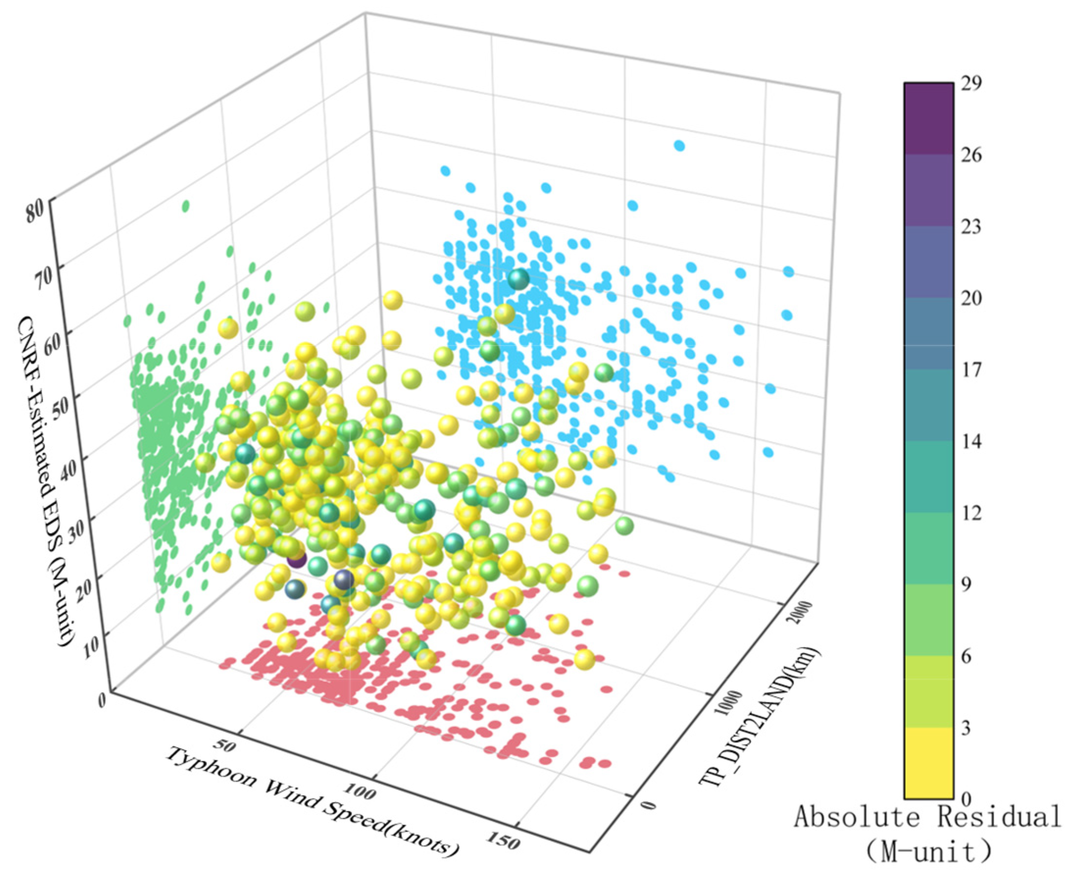
Next, the relationship between tropical cyclone descriptors and estimation performance is examined. As shown in Figure 15, the majority of samples (≈83%) fall within the wind-speed range of 25–100 knots, where the mean duct strength is 30.14 M-unit, and the mean residual is only 0.064 M-unit. In addition, about 89.4% of the observations correspond to storms located within 1000 km of the nearest mainland. For this subset, the mean duct strength reaches 30.63 M-unit, with a low mean residual of 0.202 M-unit.
Figure 15.
CNRF model residuals versus maximum sustained wind speed and TP_DIST2LAND. TP_DIST2LAND represents the distance from the tropical-cyclone center to the nearest land, as provided by the IBTrACS dataset. Point color encodes the residual magnitude.
Outside these dominant ranges, prediction errors increase. For samples beyond the 25–100-knots interval, the mean residual rises to 0.294 M-unit. When the storm distance exceeds 1000 km, the mean residual further increases to 0.717 M-unit. These patterns indicate that predictive accuracy is closely linked to both wind-speed regime and storm–land distance.
Overall, the model maintains reliable performance across a wide range of duct-strength values. Larger errors are mainly associated with weaker ducts, which are more likely to occur under reduced wind forcing or land-influenced conditions.
4.2. Temporal–Spatial Analysis
For the spatial analyses in this subsection, the regional categories were defined using the distance from each dropsonde location to the nearest coastline, denoted by . This distance was calculated from the dropsonde coordinates and coastline data and is distinct from TP_DIST2LAND, which is provided by the IBTrACS dataset and represents the distance from the tropical-cyclone center to the nearest land. The regional categories were defined as:
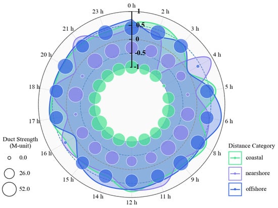
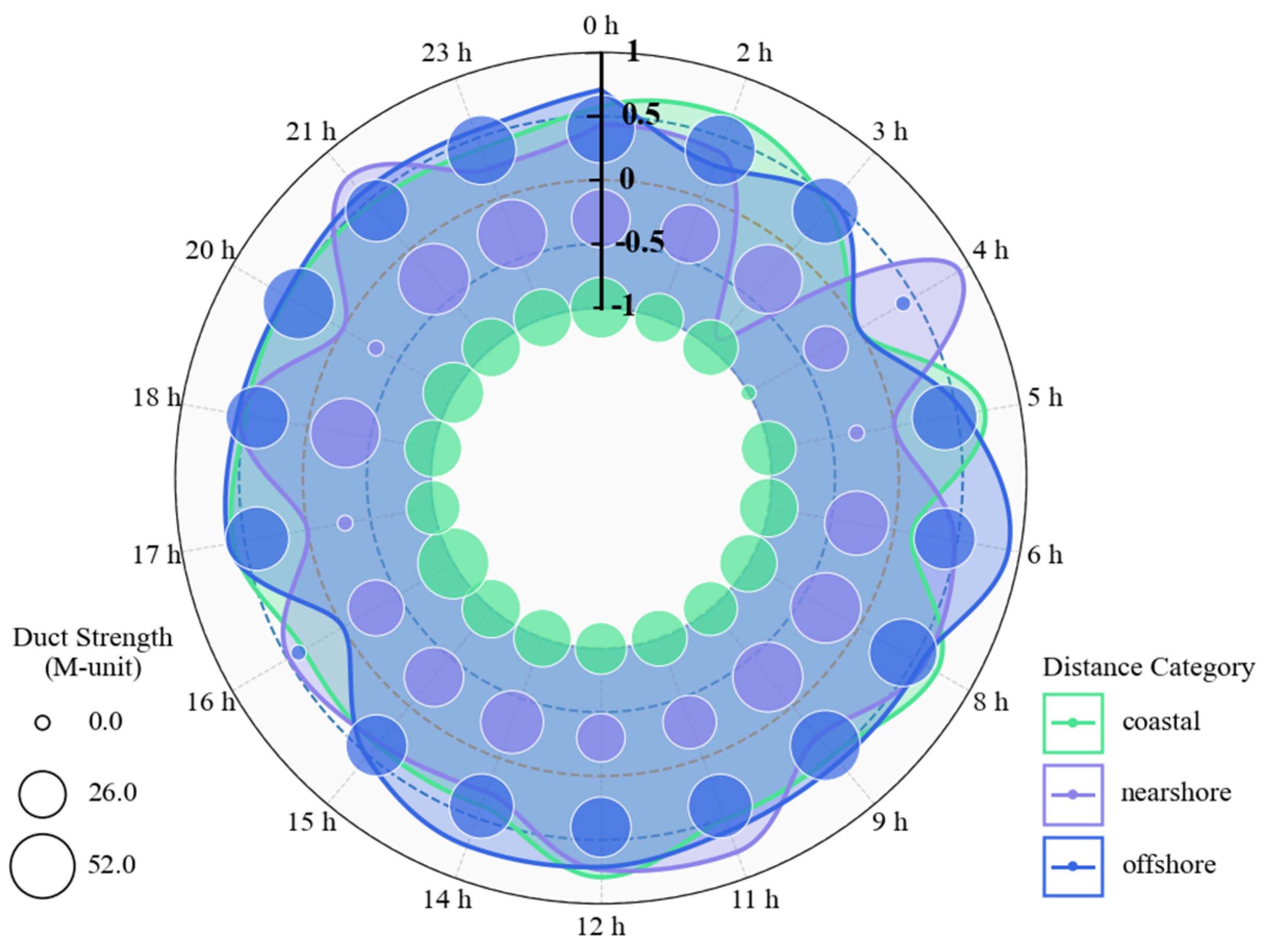
The estimation performance of the CNRF model is examined in both temporal and spatial dimensions. As shown in Figure 16, duct strength generally increases from the evening toward the hours after midnight, whereas lower values occur during the morning and at the beginning of the evening period. This behavior is consistent with the stronger nocturnal refractivity gradient, whereas RMSE also increases during the same period. The pattern is more pronounced in coastal and nearshore regions. By contrast, offshore conditions are more homogeneous, with RMSE remaining relatively balanced between 0 and 0.5 M-unit, and model performance correspondingly more stable. The enhanced diurnal variability near the coast suggests that the model is relatively sensitive to near-surface variability under tropical cyclone forcing.
Figure 16.
Diurnal variation in CNRF performance across coastal, nearshore, and offshore regions. The colored curves represent the hourly RMSE for each region, while bubble size represents the mean dropsonde-derived reference EDS.
To evaluate the sensitivity of the regional results to the selected distance thresholds, 15/150 km and 25/250 km were compared with the baseline pair of 20/200 km. The offshore subset consistently exhibited the lowest RMSE (4.865–4.979 M-unit), whereas the RMSE ranges were 5.678–5.783 M-unit for the nearshore subset and 5.779–6.276 M-unit for the coastal subset. These results confirm that the relatively stable offshore performance is robust to moderate changes in the regional thresholds. The wider RMSE variation in the coastal subset may be partly related to its smaller sample size.
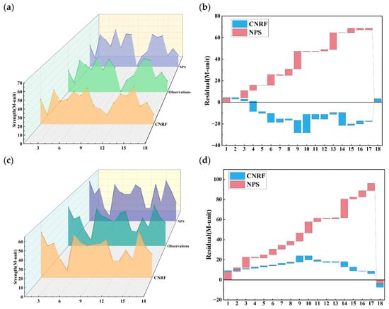
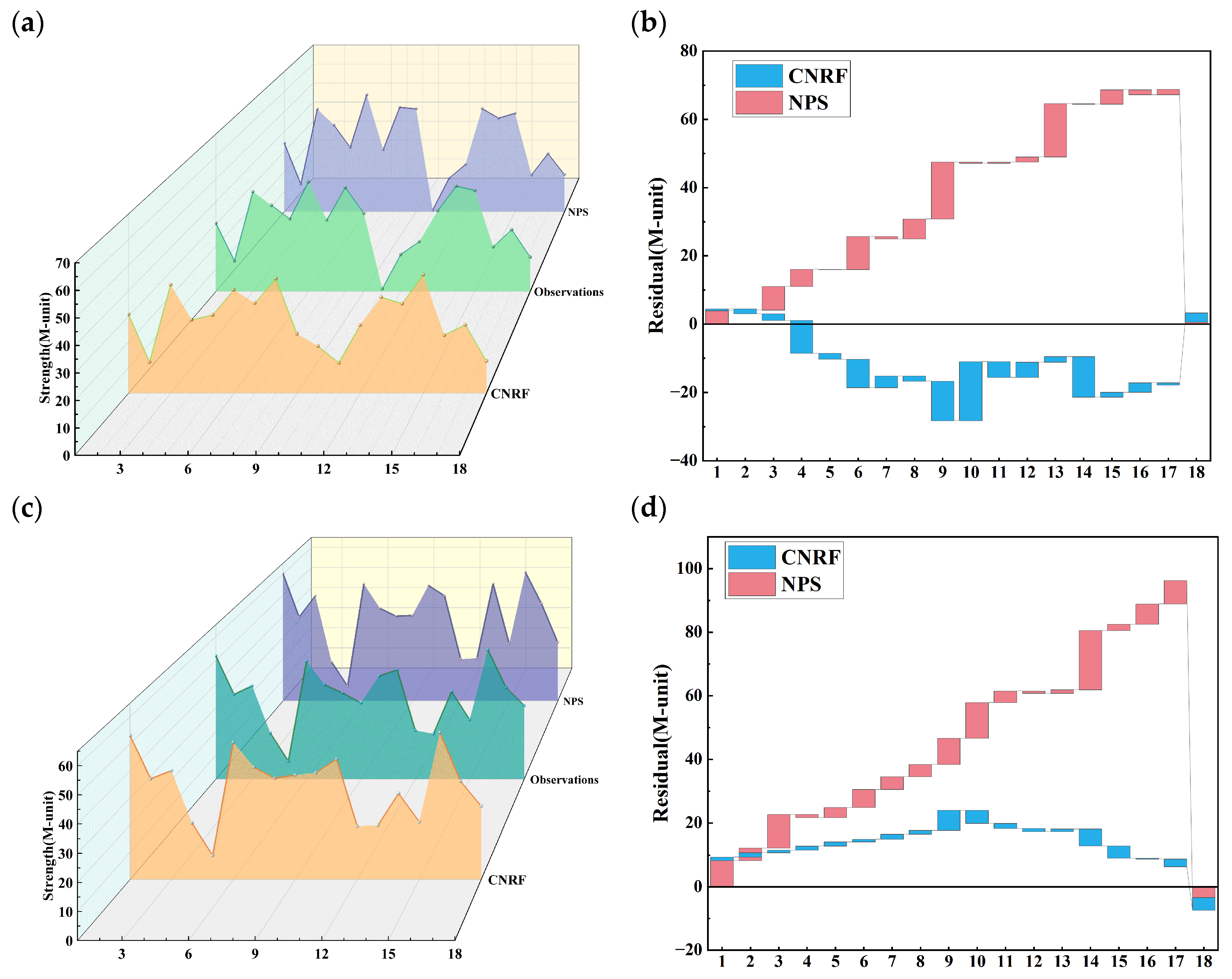
To illustrate these diurnal patterns, the dataset from 2023 was introduced as a representative example (Figure 17). Nighttime duct strength fluctuates more strongly than daytime values, while daytime conditions remain relatively stable. Across the full range of duct strengths, the CNRF model accurately tracks observed variability during both daytime and nighttime periods. Within this temporal and spatial range, the mean residual of the CNRF model is only 0.846 M-unit, compared with 4.582 M-unit for the NPS model. In addition, the RMSE of the NPS model is 6.878 on the 2023 dataset, whereas the proposed model’s RMSE is only 5.14, corresponding to a 25.3% reduction in error.
Figure 17.
Daytime and nighttime EDS in 2023: CNRF model, observations, and NPS model. (a) Duct strength for CNRF model, observations, and NPS model. (b) Residual distributions (stacked) for the daytime samples. (c) Nighttime duct strength for CNRF model, observations, and NPS model. (d) Residual distributions (stacked) for the nighttime samples.
Compared to the NPS model, the CNRF model captures day-night variations around a central tendency and stays closer to the environmental mean within comparable error bounds, while also adapting well to the enhanced refractivity gradient at night. Under both daytime and nighttime conditions, CNRF model residuals appear more symmetric and closer to a normal distribution than those of the NPS model, indicating reduced bias and more stable error performance.
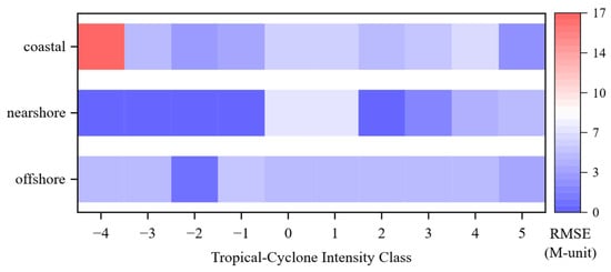
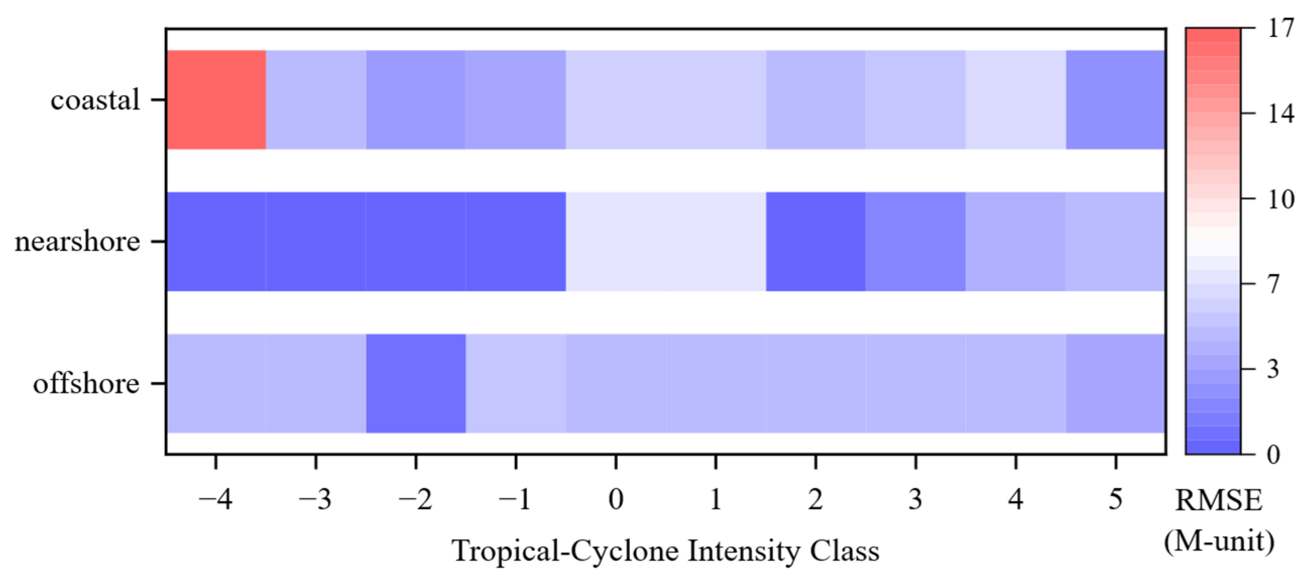
The tropical cyclone intensity class provides a direct measure of storm strength. Figure 18 shows that the CNRF model achieves low RMSE across regions for intensity classes ≥ −1, corresponding to tropical-cyclone categories ranging from tropical depressions to hurricanes. For the extreme extratropical class (−4), errors fluctuate because the coastal subset contains only one sample, and observations are limited during this transitional stage. Aside from this special case, RMSE remains low across all sea regions and intensity classes, ranging from 1.03 to 6.98 M-unit. These results indicate that the CNRF model performs stably across disturbance, tropical, and subtropical regimes.
Figure 18.
RMSE of CNRF model across tropical cyclone intensity classes. RMSE is summarized by intensity class in coastal, nearshore, and offshore regions.
4.3. Hurricane Fiona Case Analysis
To quantify the effect of incorporating tropical cyclone parameters on duct prediction, experimental observations collected near Hurricane Fiona are evaluated using the CNRF model. The Fiona dataset spans the full life cycle, from genesis to dissipation, enabling assessment across different development stages and their associated duct variability.
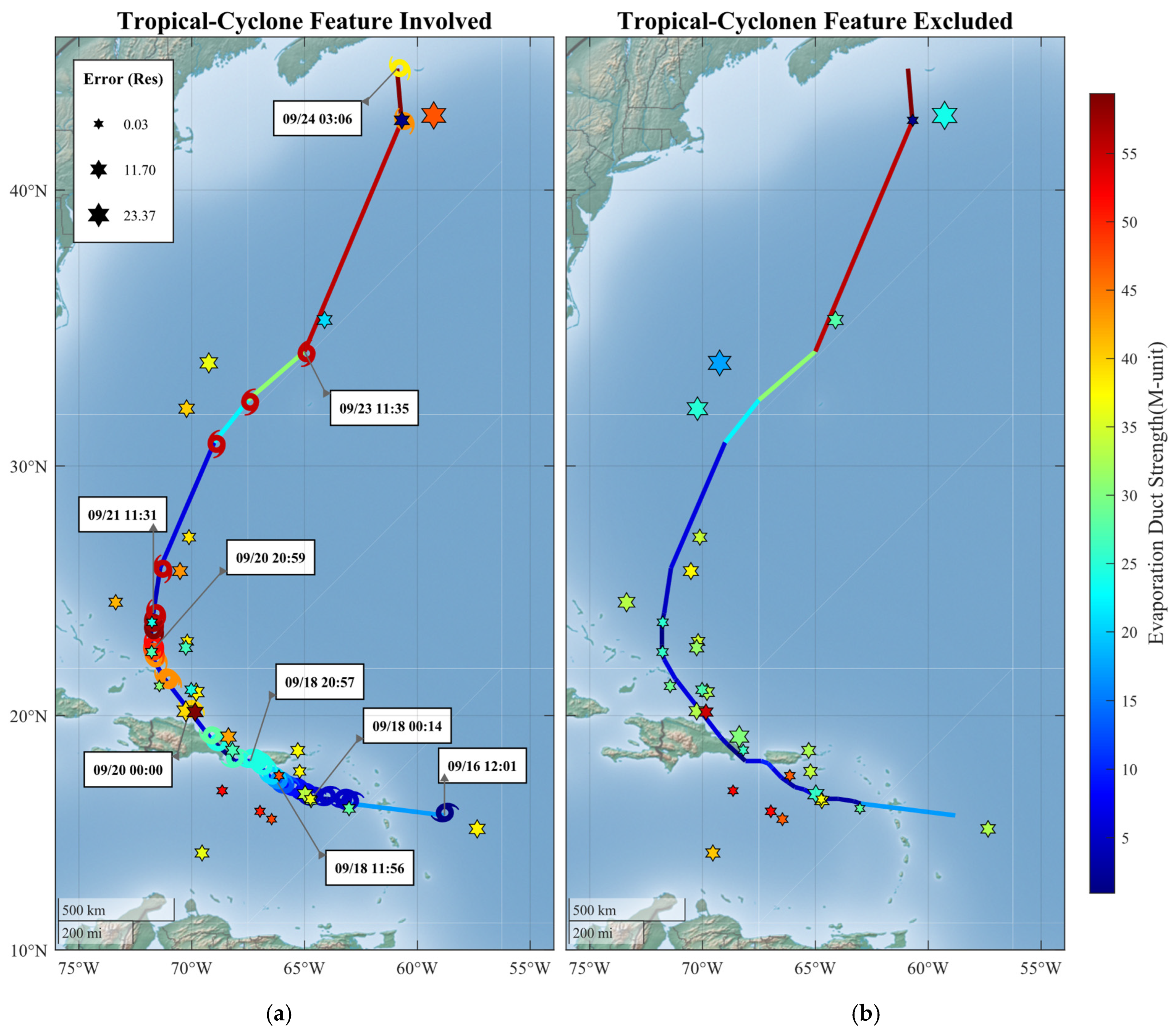
Validation using Hurricane Fiona confirms the model’s adaptability throughout the entire storm life cycle (Figure 19). Along the week-long track, the model maintains low errors in both time and space. Estimation accuracy remains stable during the intensification stage, when meteorological conditions change rapidly. Reliable performance is also achieved at locations with stronger central winds and at sampling points farther from the storm track. Including tropical cyclone descriptors leads to a clear improvement in estimation performance. RMSE decreases from 7.543 to 6.260 M-unit, corresponding to a reduction of 17.0%. Meanwhile, R2 increases from 0.523 to 0.671, corresponding to an absolute increase of 0.148, and the residual error decreases by 22.4% from an initial value of 3.475 M-unit. The improvement is evident both near the storm core and at off-track locations under high storm-motion conditions. These results demonstrate that explicit tropical cyclone information enhances the robustness of evaporation-duct prediction under rapidly evolving tropical cyclone environments.
Figure 19.
Validation results for Hurricane Fiona using the CNRF models with and without tropical-cyclone descriptors. Panel (a) includes tropical-cyclone descriptors, whereas panel (b) excludes them. Hexagon color encodes duct strength, and hexagon size encodes prediction error.
5. Conclusions
This study focuses on quantifying the relationship between EDS under tropical cyclone conditions and tropical cyclone descriptors. Dropsonde-derived meteorological variables are integrated with best-track tropical cyclone records to analyze events from 1996 to 2024 across the Northeast Pacific and North Atlantic. An integrated framework proposed in this study, termed the CNRF model, is used to predict EDS by incorporating tropical cyclone wind speed, intensity class, distance to the nearest coastline, and selected near-surface meteorological features. Compared to the NPS numerical model, the CNRF model reduces RMSE from 6.996 to 5.350 M-unit, corresponding to a reduction of about 23.5%. The contribution of tropical-cyclone descriptors is more directly demonstrated by the within-framework ablation experiment, in which the data, model structure, and evaluation procedure were kept unchanged. Incorporating tropical-cyclone descriptors reduced the RMSE from 6.282 to 5.350 M-unit for the overall test set and from 7.543 to 6.260 M-unit for the independent Hurricane Fiona case, corresponding to reductions of approximately 14.8% and 17.0%, respectively. This controlled comparison identifies the additional information provided by tropical-cyclone descriptors, rather than the use of any individual learning algorithm, as the principal contribution of the proposed framework.
These findings indicate that tropical-cyclone descriptors provide useful information for characterizing EDS variability under extreme weather conditions and for supporting EDS estimation in tropical-cyclone-affected environments. Nevertheless, the present dataset remains limited in spatial and environmental coverage, the reported performance is based on a single event-level held-out test set, and the current framework uses contemporaneous rather than lead-time inputs. In addition, although EDH is used to diagnose the duct layer and derive EDS, EDH and EDS are not modeled jointly. Future work will therefore focus on joint EDH–EDS modeling and validation using observations from additional oceanic regions to assess the framework’s applicability across a broader range of environmental conditions.
Author Contributions
Conceptualization, J.W. and C.Y.; methodology, J.M., W.L. and J.S.; software, J.M. and W.L.; validation, C.Y.; formal analysis, C.Y. and J.S.; investigation, J.W. and C.Y.; resources, C.Y.; data curation, J.M., W.L. and J.S.; writing—original draft preparation, J.M.; writing—review and editing, J.W. and W.L.; visualization, J.M., W.L. and J.S.; supervision, J.W. and C.Y.; project administration, C.Y.; funding acquisition, J.W. All authors have read and agreed to the published version of the manuscript.
Funding
This work was supported in part by the National Natural Science Foundation of China 62031008.
Data Availability Statement
The datasets analyzed in this study were derived from publicly available resources. Tropical cyclone data were obtained from IBTrACS, available from the NOAA National Centers for Environmental Information at https://www.ncei.noaa.gov/products/international-best-track-archive (accessed on 12 March 2025). Dropsonde data were obtained from the NOAA AOML data products, available at https://www.aoml.noaa.gov/data-products/ (accessed on 16 February 2025). Sea-surface meteorological parameters were obtained from dataset D094001 in the Geoscience Data Exchange (GDEX) of the National Center for Atmospheric Research (NCAR), managed by the University Corporation for Atmospheric Research (UCAR), and are available at https://gdex.ucar.edu/datasets/d094001/dataaccess/ (accessed on 21 March 2025).
Conflicts of Interest
The authors declare no conflicts of interest.
References
- 6G Mobile Wireless Networks; Wu, Y., Singh, S., Taleb, T., Roy, A., Dhillon, H.S., Kanagarathinam, M.R., De, A., Eds.; Computer Communications and Networks; Springer International Publishing: Cham, Switzerland, 2021; ISBN 978-3-030-72776-5. [Google Scholar]
- Wang, J.; Zhou, H.; Li, Y.; Sun, Q.; Wu, Y.; Jin, S.; Quek, T.Q.; Xu, C. Wireless Channel Models for Maritime Communications. IEEE Access 2018, 6, 68070–68088. [Google Scholar] [CrossRef] [Scilit]
- Ji, H.; Zhang, J.; Guo, L.; Wei, Y.; Leng, J.; Zhang, Y.; Li, Q.; Guo, X.; Zhang, Y. DenseRefrception: A Densely Connected Perception Framework for Passive Retrieval of Ocean Refractive Environments via GPS Scattered Signals. IEEE Trans. Geosci. Remote Sens. 2026, 64, 2001719. [Google Scholar] [CrossRef] [Scilit]
- Wu, J.; Wei, Z.; Liu, C.; Ma, Q.; Wei, Z.; Cui, T.; Li, Q.; Wu, X.; Ye, J.; Wu, S.; et al. Ad-SACNet: Spatial Attention Compression Network for Atmospheric Duct Inversion with Radar Sea Clutter Data. IEEE Trans. Antennas Propag. 2026, 74, 7967–7981. [Google Scholar] [CrossRef] [Scilit]
- Kang, S.; Zhang, Y.; Wang, H. Atmospheric Duct in Troposphere Environment; Science Press: Beijing, China, 2014. [Google Scholar]
- Yang, C.; Wang, J. The Investigation of Cooperation Diversity for Communication Exploiting Evaporation Ducts in the South China Sea. IEEE Trans. Antennas Propag. 2022, 70, 8337–8347. [Google Scholar] [CrossRef] [Scilit]
- Liu, C.; Pan, Z.; Guo, L. Statistical Analysis of Occurrence and Characteristics of Atmospheric Ducts in China. Chin. J. Radio Sci. 1996, 11, 60–66. [Google Scholar]
- Cheng, Y.; Zhou, S.; Wang, D.; Lu, Y.; Huang, K.; Yao, J.; You, X. Observed Characteristics of Atmospheric Ducts over the South China Sea in Autumn. Chin. J. Oceanol. Limnol. 2016, 34, 619–628. [Google Scholar] [CrossRef] [Scilit]
- Wang, H.; Wu, Z.; Kang, S.; Zhao, Z. Monitoring the Marine Atmospheric Refractivity Profiles by Ground-Based GPS Occultation. IEEE Geosci. Remote Sens. Lett. 2013, 10, 962–965. [Google Scholar] [CrossRef] [Scilit]
- Jeske, H. Modern Topics in Microwave Propagation and Air-Sea Interaction. In State and Limits of Prediction Methods, of Radar Wave Propagation Conditions over the Sea; Reidel Publishers: Dordrecht, The Netherlands, 1973; p. 131. [Google Scholar]
- Paulus, R.A. Practical Application of an Evaporation Duct Model. Radio Sci. 1985, 20, 887–896. [Google Scholar] [CrossRef] [Scilit]
- Liu, W.T.; Katsaros, K.B.; Businger, J.A. Bulk Parameterization of Air-Sea Exchanges of Heat and Water Vapor Including the Molecular Constraints at the Interface. J. Atmos. Sci. 1979, 36, 1722–1735. [Google Scholar] [CrossRef] [Scilit]
- Babin, S.M.; Young, G.S.; Carton, J.A. A New Model of the Oceanic Evaporation Duct. J. Appl. Meteorol. 1997, 36, 193–204. [Google Scholar] [CrossRef] [Scilit]
- Frederickson, P.; Davidson, K.; Goroch, A. Operational Bulk Evaporation Duct Model for MORIAH; Version 1.2; Technical Report; Naval Postgraduate School: Monterey, CA, USA, 2000. [Google Scholar]
- Wu, J.; Zhang, J.; Zhang, Y.; Wei, Z. Research on Inversion Method of Range Direction Inhomogeneous Evaporation Duct Based on Deep Learning. Chin. J. Radio Sci. 2023, 38, 665–672. [Google Scholar]
- Liu, W.; Wang, J.; Yang, C. A Short-Term Forecasting Model of Elevated Duct Based on the Long Short-Term Memory Network. In Proceedings of the 2024 IEEE 12th Asia-Pacific Conference on Antennas and Propagation (APCAP), Nanjing, China, 22–25 September 2024; IEEE: New York, NY, USA, 2024; pp. 1–2. [Google Scholar]
- Wang, S.; Yang, K.; Shi, Y.; Yang, F. Observations of Anomalous Over-the-Horizon Propagation in the Evaporation Duct Induced by Typhoon Kompasu (202118). IEEE Antennas Wirel. Propag. Lett. 2022, 21, 963–967. [Google Scholar] [CrossRef] [Scilit]
- Wang, S.; Yang, K.; Shi, Y.; Yang, F.; Zhang, H. Observed Over-the-Horizon Propagation Characteristics and Evaporation Duct Inversion During the Entire Process of Tropical Cyclone Mulan (202207). IEEE Trans. Antennas Propag. 2023, 71, 5322–5334. [Google Scholar] [CrossRef] [Scilit]
- Xiaohan, L.; Qiushuang, Y.; Chenqing, F.; Jie, Z. Deep Learning-Based Sea Surface Wind Speed Retrieval Method for Sentinel-1 Dual-Polarimetric SAR under Typhoon Sea State. Chin. J. Radio Sci. 2024, 39, 1095–1101. [Google Scholar]
- Greenway, D.P.; Vaughan, A.E.; Kammerer, A.J.; Hackett, E.E. Characterizing Range-Dependent Variations of the Evaporation Duct: A Meteorological Perspective. IEEE Trans. Antennas Propag. 2024, 72, 7239–7251. [Google Scholar] [CrossRef] [Scilit]
- Yang, N.; Song, D.; Lu, T.; Su, D.; Wang, T. The Evaporation Duct Characteristics of Typhoon Kompasu (202118) Based on Buoys Observation. IEEE Antennas Wirel. Propag. Lett. 2024, 24, 212–216. [Google Scholar] [CrossRef] [Scilit]
- Knapp, K.R.; Kruk, M.C.; Levinson, D.H.; Diamond, H.J.; Neumann, C.J. The International Best Track Archive for Climate Stewardship (IBTrACS) Unifying Tropical Cyclone Data. Bull. Am. Meteorol. Soc. 2010, 91, 363–376. [Google Scholar]
- Gahtan, J.; Knapp, K.R.; Schreck, C.J., III; Diamond, H.J.; Kossin, J.P.; Kruk, M.C. International Best Track Archive for Climate Stewardship (IBTrACS) Project, Version 4r01; NOAA National Centers for Environmental Information: Asheville, NC, USA, 2024. [Google Scholar]
- Bean, B.R.; Dutton, E.J. Radio Meteorology; National Bureau of Standards Monograph 92; U.S. Government Printing Office: Washington, DC, USA, 1966. [Google Scholar]
- ITU-R P. 453-14; The Radio Refractive Index: Its Formula and Refractivity Data. The International Telecommunication Union (ITU): Geneva, Switzerland, 2019.
- Babin, S.M.; Dockery, G.D. LKB-Based Evaporation Duct Model Comparison with Buoy Data. J. Appl. Meteorol. 2002, 41, 434–446. [Google Scholar] [CrossRef] [Scilit]
- Babin, S.M.; Dockery, G.D. Development and Experimental Evaluation of Oceanic Evaporation Duct Models Based on the LKB Approach; Final Report; Johns Hopkins University Applied Physics Laboratory: Laurel, MD, USA, 2001. [Google Scholar]
- Shi, Y.; Zhang, Q.; Wang, S.; Yang, K.; Yang, Y.; Ma, Y. Impact of typhoon on evaporation duct in the Northwest Pacific Ocean. IEEE Access 2019, 7, 109111–109119. [Google Scholar] [CrossRef] [Scilit]
- Shi, Y.; Zhang, Q.; Wang, S.; Yang, K.; Yang, Y.; Yan, X.; Ma, Y. A comprehensive study on maximum wavelength of electromagnetic propagation in different evaporation ducts. IEEE Access 2019, 7, 82308–82319. [Google Scholar] [CrossRef] [Scilit]
- Data—NOAA/AOML. Available online: https://www.aoml.noaa.gov/data-products/ (accessed on 9 April 2026).
- National Centers for Environmental Prediction. NCEP Climate Forecast System Version 2 (CFSv2) Selected Hourly Time-Series Products; Research Data Archive at NSF NCAR GDEX: Boulder, CO, USA, 2011.
- International Best Track Archive for Climate Stewardship (IBTrACS). Available online: https://www.ncei.noaa.gov/products/international-best-track-archive (accessed on 9 April 2026).
- Prokhorenkova, L.; Gusev, G.; Vorobev, A.; Dorogush, A.V.; Gulin, A. CatBoost: Unbiased Boosting with Categorical Features. Adv. Neural Inf. Process. Syst. 2018, 31, 6639–6649. [Google Scholar] [CrossRef] [Scilit]
- Duan, T.; Anand, A.; Ding, D.Y.; Thai, K.K.; Basu, S.; Ng, A.; Schuler, A. Ngboost: Natural Gradient Boosting for Probabilistic Prediction. In Proceedings of the 37th International Conference on Machine Learning, Virtual, 13–18 July 2020; PMLR: Birmingham, UK, 2020; pp. 2690–2700. [Google Scholar]
- Singh, J.; Banerjee, R. A Study on Single and Multi-Layer Perceptron Neural Network. In Proceedings of the 2019 3rd International Conference on Computing Methodologies and Communication (ICCMC), Erode, India, 27–29 March 2019; IEEE: New York, NY, USA, 2019; pp. 35–40. [Google Scholar]
Disclaimer/Publisher’s Note: The statements, opinions and data contained in all publications are solely those of the individual author(s) and contributor(s) and not of MDPI and/or the editor(s). MDPI and/or the editor(s) disclaim responsibility for any injury to people or property resulting from any ideas, methods, instructions or products referred to in the content. |
© 2026 by the authors. Licensee MDPI, Basel, Switzerland. This article is an open access article distributed under the terms and conditions of the Creative Commons Attribution (CC BY) license.