


Highlights
What are the main findings?
- A miniaturized dual-channel airborne imaging spectrometer with a self-collimating shared-optical-path configuration is proposed, and the design is predicted to support simultaneous observation of SIF-related spectral radiance and vegetation-canopy spectral reflectance without inter-channel temporal delay.
- An asymmetric double Babinet depolarizer is incorporated into the optical design, and simulations indicate reduced system polarization sensitivity, thereby supporting improved spectral-measurement accuracy.
What are the implications of the main findings?
- The proposed optical configuration provides a compact and integrated design strategy for airborne SIF spectral imaging systems and offers a design-stage basis for future dynamic monitoring of vegetation physiological status at regional scales.
- The proposed instrument concept is expected to support fine-scale airborne observations of vegetation ecology and has potential applications in near-surface validation of spaceborne fluorescence products.
Abstract
Solar-induced chlorophyll fluorescence (SIF) provides a direct proxy for vegetation photosynthesis-related information; however, under stress conditions, its relationship with photosynthesis should be interpreted together with absorbed photosynthetically active radiation by chlorophyll (APARchl) and non-photochemical quenching (NPQ). This study presents a conceptual design of a compact dual-channel airborne imaging spectrometer for synchronous observation of SIF-related spectral radiance and broadband vegetation-canopy spectral reflectance (BR). A self-collimating shared-optical-path configuration is proposed to reduce the system volume, yielding a simulated optical envelope of 205 × 150 × 120 mm3. Optical simulations predict spectral resolutions better than 0.3 nm over 670–780 nm for the SIF channel and better than 2 nm over 400–780 nm for the BR channel. An asymmetric double Babinet depolarizer is incorporated to reduce polarization-related errors, and the simulated system polarization sensitivity is below 1%. The calculated stray-light ratios of the SIF and BR channels are 0.553% and 0.287%, respectively. LightTools was used to simulate the radiative transfer performance of the instrument under realistic scenes. Furthermore, an end-to-end SIF retrieval simulation was performed to evaluate the retrieval capability of the proposed system. The results indicate that the proposed concept is theoretically feasible and may support future quantitative SIF retrieval and the interpretation of vegetation photosynthetic and stress-related processes.
1. Introduction
In regional-to-global assessments of vegetation photosynthesis, vegetation indices such as the normalized difference vegetation index (NDVI) and leaf area index (LAI) have long been used as proxies for photosynthetic productivity [1,2]. However, these metrics are indirectly linked to the underlying physiological processes. Numerous studies have shown that growing seasons derived from NDVI or LAI are often significantly longer than those inferred from gross primary productivity (GPP) or flux-based observations [3,4]. In contrast, solar-induced chlorophyll fluorescence (SIF) originates directly from the energy partitioning processes of photosynthesis; therefore, it serves as a more physiologically meaningful indicator of photosynthetic activity.
SIF arises from the re-emission of the fraction of absorbed photosynthetically active radiation that is not utilized in photochemistry or dissipated via non-photochemical quenching (NPQ). Studies from leaf to canopy scales consistently demonstrate a positive correlation between SIF and photosynthetic activity [5,6]. As illustrated in Figure 1, SIF acts as a direct, non-invasive probe of photosynthesis, characterizing the efficiency of photosynthetic electron transport and the state of light energy utilization. It is highly sensitive to functional changes induced by light, temperature, and water stress, and can reveal drought-driven declines in photosynthesis prior to observable canopy structural responses [7,8]. Consequently, SIF outperforms traditional vegetation indices in capturing the spatiotemporal dynamics of photosynthesis and in assessing ecosystem responses to climate variability and environmental stress, and has become a key parameter in global carbon cycle monitoring and functional vegetation remote sensing.
Figure 1.
Relationship between SIF and vegetation ecology.
Under non-stress conditions, SIF is positively correlated with the photosynthetic rate and can serve as an indicator of photosynthetic productivity. However, under stress conditions such as high irradiance, drought, and low temperature, the SIF signal is jointly regulated by photochemical quenching (PQ) and NPQ. During mild drought, vegetation typically enhances photoprotective processes by upregulating NPQ, thereby increasing thermal dissipation, reducing chlorophyll fluorescence quantum yield, and suppressing SIF. In contrast, the response of photosynthetic productivity to drought is often delayed or relatively weak due to the combined effects of irradiance variability and stomatal regulation. Consequently, if NPQ is not considered, reductions in SIF may be erroneously interpreted as declines in photosynthetic productivity. Moreover, fluorescence radiance is driven by incident illumination and is fundamentally determined by absorbed photosynthetically active radiation by chlorophyll (APARchl). Accurate retrieval of fluorescence quantum efficiency therefore requires effective separation of chlorophyll absorption from that of other vegetation components. Based on the spectral absorption characteristics of chlorophyll, this requirement has motivated a focus on the 400–500 nm and 600–700 nm spectral regions [9]. Accordingly, to better interpret the relationships among SIF, plant photosynthesis, and stress-related responses, an additional spectral channel is required to provide broadband spectral reflectance information, which is expected to support the estimation of NPQ- and APARchl-related processes [10].
SIF remote sensing platforms mainly include ground-based, airborne, and spaceborne systems. At present, satellite observations are largely constrained by coarse spatial resolution, discontinuous spatial sampling, and long revisit cycles, making them inadequate for high-precision, dynamic SIF monitoring at regional scales. For example, the Tropospheric Monitoring Instrument (TROPOMI) onboard Sentinel-5P [11] provides daily global coverage. During the initial mission phase, its spatial resolution was 3.5 × 7 km, which was insufficient to resolve fine-scale heterogeneity within croplands and forested areas. The dedicated SIF payload, the Solar-Induced Chlorophyll Fluorescence Imaging Spectrometer (SIFIS) [12], has a swath width of 34 km and requires 1–2 months to achieve global coverage. Although ground-based or laboratory instruments offer high accuracy, their site-based monitoring provides limited spatial coverage. In this context, lightweight and compact airborne SIF imaging spectrometers are expected to bridge the scale gap between satellite and ground-based observations and, when combined with flexible flight strategies, support fine-scale spatiotemporal characterization of ecosystem carbon-water coupling processes.
Among currently mature airborne SIF remote sensing systems, the High-Performance airborne imaging spectrometer (HyPlant) [13] is one of the few capable of simultaneously acquiring SIF and vegetation canopy spectral reflectance. The system consists of two independent spectrometers, and the SIF module alone weighs 25 kg, imposing stringent constraints on payload capacity and flight endurance. In contrast, the Chlorophyll Fluorescence Imaging Spectrometer (CFIS) [14], the fluorescence imaging of red and far-red light yield (FIREFLY) [15], and the imaging spectrometer developed by Yu et al. [16] primarily provide fluorescence spectral information, but lack synchronous acquisition of key parameters such as canopy reflectance. The main parameters of these instruments are summarized in Table 1.
Table 1.
Airborne SIF imaging spectrometer systems.
Additionally, since imaging spectrometers employ components such as gratings and mirrors that exhibit strong polarization sensitivity, the instrument response is determined not only by the target radiance but also by the polarization state of the incident light. Solar radiation becomes polarized or partially polarized after scattering by atmospheric molecules and aerosols [17], while specular reflection from the leaf cuticle/wax layer introduces pronounced partial linear polarization [18]. These effects make the polarization-dependent response of imaging spectrometers more prominent, directly degrading the accuracy of radiometric measurements and retrievals [19]. Moreover, stray light is another major error source contributing to uncertainty in SIF radiance measurements. Therefore, to ensure measurement accuracy, the system design should incorporate both polarization-sensitivity control and stray-light suppression.
To address these challenges, this study presents a conceptual design of a compact airborne dual-channel imaging spectrometer intended for the synchronous observation of vegetation-canopy spectral radiance and spectral reflectance. One channel is dedicated to SIF detection, while the reflectance channel provides spectral information that may support the estimation of NPQ- and APARchl-related processes. Based on the optical path of the SIF channel, a self-collimating configuration is introduced to reduce optical volume. To ensure radiometric accuracy, an asymmetric double Babinet depolarizer is designed for system-level depolarization. LightTools is used to simulate the radiative transfer performance of the instrument. The scope of this paper is limited to initial optical design and feasibility analysis, including optical system evaluation, simulated stray-light analysis, theoretical signal-to-noise ratio (SNR) calculation and end-to-end simulation of SIF retrieval. The main contents of this paper include optical system design and evaluation, stray-light analysis and suppression, and theoretical SNR analysis. Section 2 describes the observation objectives and requirements of the shared-optical-path dual-channel imaging spectrometer. Section 3 presents the optical design methodology and results. Section 4 analyzes the stray light, theoretical SNR and SIF-retrieval simulation of the proposed instrument. Section 5 discusses the results, and Section 6 concludes the study.
2. System Design Specifications
2.1. Requirement Analysis of the SIF Channel
SIF retrieval is challenged by its weak signal and its superposition on canopy-reflected radiance [20]. Therefore, absorption dark lines in the solar irradiance spectrum are commonly used for SIF extraction. Within an absorption line, the incident solar irradiance and vegetation-reflected radiance are relatively reduced, while the filling-in effect caused by fluorescence becomes more pronounced, providing favorable conditions for SIF retrieval. The observation principle of SIF and broadband reflectance signals is shown in Figure 2.
Figure 2.
Observation principle of SIF and broadband reflectance signals.
The classical SIF retrieval algorithm, Fraunhofer Line Discrimination (FLD) [21], uses the apparent radiances of two spectral bands: one located inside the Fraunhofer line and the other outside the Fraunhofer line, denoted as and , respectively. When these two bands are sufficiently close, the vegetation reflectance and fluorescence value are assumed to remain approximately constant between them. Once the incident solar irradiance and the canopy upwelling radiance are known, the fluorescence signal can be derived as follows:
where and represent the incident solar irradiance inside and outside the Fraunhofer line, respectively. The radiance of the vegetation target can be directly obtained using the instrument after laboratory radiometric calibration, while the incident solar irradiance can be inversely derived from pre-flight measurements of a standard diffuse reflectance panel with known reflectance.
SIF is an electromagnetic signal emitted by chlorophyll-a in green leaves within the spectral range of 650–800 nm. In this range, there are several narrow atmospheric absorption lines and solar Fraunhofer lines (0.1–10 nm) [22,23]. The absorption windows centered at 687 nm (-B) and 760 nm (-A) nearly overlap with the SIF emission spectrum. Moreover, retrieval methods based on atmospheric absorption lines generally show better stability and applicability. Therefore, the instrument design in this study is based on the atmospheric oxygen absorption bands. To avoid the effects of water vapor absorption at the upper end of this spectral interval, the spectral range of the SIF channel is selected as 670–780 nm.
The detection and retrieval of weak SIF signals place stringent requirements on the spectral resolution (SR) and SNR of the instrument [24]. Previous studies have carried out extensive field experiments to determine the optimal SR for SIF detection and retrieval [25]. The results show that the best separability between fluorescence emission and background reflectance is achieved with an SR of approximately 0.3 nm. Here, SR represents the minimum spectral feature width that can be resolved by the instrument. In contrast, the spectral sampling interval (SSI) defines the wavelength spacing between adjacent detector spectral samples. To avoid spectral aliasing in the measured signal, an SSI of 0.1 nm was selected considering the characteristic shape of the spectral radiance curves within the spectral range covered by the instrument.
The SNR requirement for high-precision SIF retrieval depends on the required accuracy of vegetation fluorescence measurements. The FLEX mission proposed that SIF should be retrieved with a measurement accuracy of 10%, and extensive algorithm and model studies were conducted to determine the optimal SNR values. The results show that, for one spatial sampling distance (SSD), an SSI of 0.1 nm, and typical vegetation radiance at the top of atmosphere (TOA), the minimum SNR requirements are 115 in the -A window and 175 in the -B window. These values can be converted to equivalent minimum SNR requirements of approximately 200 and 303 at an SR of 0.3 nm according to the relationship . Based on this conversion, the minimum SNR requirement of the proposed instrument is defined in this study.
2.2. Requirement Analysis of the BR Channel
Vegetation stress mainly refers to disturbances in photosynthetic function caused by biotic or abiotic factors, including drought, excessive illumination, temperature variations, water-balance abnormalities, pests, and diseases. These stress factors can alter plant photochemical utilization, fluorescence emission, and NPQ processes, and therefore can be reflected in optical indicators such as SIF and canopy reflectance.
The photochemical reflectance index (PRI) has a clear and direct relationship with NPQ, and can be used to quantitatively characterize NPQ-related heat dissipation [26]. PRI is defined as the normalized difference between the reflectance at 531 nm and 570 nm. The subtle spectral variation near 531 nm is closely related to the physiological status of vegetation; therefore, PRI is sensitive to wavelength position and spectral bandwidth. Previous studies have shown that an SSI of 1 nm is sufficient for PRI extraction [27]. To reduce the influence of canopy structure, such as leaf inclination angle, on narrow-band reflectance measurements, it is necessary to measure the full spectral dynamic variation over the 500–600 nm range [25].
In vegetation reflectance spectra, the red edge within 680–760 nm, together with its position and slope, is highly sensitive to variations in chlorophyll content and canopy absorbed photosynthetically active radiation (APAR), and can provide constraints on the radiative transfer and absorption background of fluorescence signals [28,29].
In summary, to better support the potential interpretation of dynamic fluorescence variations in relation to actual photosynthetic activity and vegetation health status, a canopy-reflectance observation channel synchronized with the SIF channel is required to acquire canopy spectral reflectance over 400–780 nm. Since the red edge and chlorophyll absorption features in vegetation reflectance spectra are broad spectral features, an SR of 2 nm and an SSI of 0.66 nm are sufficient to meet the measurement requirements.
The observation objectives of each spectral band of the dual-channel imaging spectrometer studied in this paper are summarized in Table 2.
Table 2.
Characteristic spectral bands of the two channels and their corresponding observation targets.
The primary design challenge lies in the fluorescence channel. To simultaneously achieve high SNR and sub-nanometer SR, a large numerical aperture is required; here, an F-number of 2.2 is adopted. The instrument is designed as a UAV-borne push-broom imaging spectrometer consisting of a telescope module and a spectrometer module, with a system magnification of 1. To ensure radiometric accuracy, system specifications for polarization sensitivity and stray light are defined in accordance with the requirements of the Fluorescence Explorer (FLEX) mission of the European Space Agency (ESA) [25]. The detailed design parameters are listed in Table 3.
Table 3.
Design parameters of the dual-channel imaging spectrometer.
3. Optical System Design
3.1. Telescope System
The requirements for high SNR and miniaturization impose stringent constraints on the telescope performance. An off-axis two-mirror configuration is adopted due to its unobscured aperture, compact structure, near-diffraction-limited imaging performance, image-space telecentricity, and large relative aperture with high light-gathering capability. As an all-reflective system, it eliminates chromatic aberration and reduces energy loss compared with transmissive designs. The main design parameters are listed in Table 4.
Table 4.
Design parameters of telescope system.
After theoretical analysis and optimization, the system meets the design specifications with excellent imaging quality. The three-dimensional model exported from ZEMAX is shown in Figure 3a.
Figure 3.
(a) Three-dimensional model of the telescope system, (b) MTF curves, and (c) spot diagram.
The modulation transfer function (MTF) is used to evaluate telescope imaging performance. The system Nyquist frequency is calculated as [30]
where is the detector pixel size (µm). Considering 6-pixel binning in the spatial dimension, is set to 8 cycles/mm. As shown in Figure 3b,c, the MTF of the telescope exceeds 0.9 at the Nyquist frequency, and the RMS spot radii for all five fields are below 2 µm, demonstrating excellent imaging performance.
3.2. Asymmetric Double Babinet Depolarizer Analysis
To mitigate the impact of the incident polarization state on the instrument response, a depolarizer is typically placed in the fore-optics to minimize measurement errors caused by the polarization sensitivity of optical components. Given the SIF channel’s high SR of 0.3 nm, we employ a double Babinet depolarizer to achieve broadband depolarization across the full spectral range for all polarization states. A conventional double Babinet depolarizer consists of two identical horizontal-vertical (H-V) depolarizer pairs, denoted as H-V-1 and H-V-2, whose optical axes are rotated by 45° relative to each other. The wedge angles of H-V-1 and H-V-2 are denoted by and , respectively.
Owing to crystal birefringence, a single object point is split into four image points after passing through the depolarizer, as shown in Figure 4b, which degrades the imaging quality of the instrument. In the spectrometer designed in this study, the spectral pixels remain unbinned with a pixel size of 11 µm, whereas the spatial pixels are binned to 66 µm. Therefore, the depolarizer is rotated by 45° about the z-axis so that the short axis (H1) of the parallelogram formed by the four images is aligned with the spectral dimension, as shown in Figure 4c, thereby reducing the influence of image separation on the spectral dimension. Increasing and improves the depolarization performance, but also leads to increases in H1 and H2, respectively. Therefore, an asymmetric double Babinet depolarizer [31], namely , is adopted to balance depolarization performance and image quality.
Figure 4.
Schematic of spot separation after a double Babinet depolarizer: (a) incident object point; (b) four separated image points; (c) spot distribution after rotating the depolarizer by 45°.
The Mueller matrix of a conventional double Babinet depolarizer has been derived in detail in [32]. For the asymmetric configuration, the average Mueller matrix can be obtained from the Mueller matrix of the H-V depolarizer combined with rotation matrices and pupil integration:
where represents the first-order Bessel function, and are defined in Equation (4).
denotes the birefringence of the material at a given wavelength ; is the entrance pupil radius.
To limit image degradation, the separation between the o- and e-rays on the detector is constrained to be less than half a pixel [31]. With a single spectral pixel size µm, the condition becomes
where is the telescope focal length. Quartz was selected as the depolarizer material; its birefringence dispersion curve is shown in Figure 5a.
Figure 5.
(a) Birefringence of quartz; (b) residual degree of polarization curves for linearly polarized light at different polarization angles versus wavelength.
For the system designed in this study, the entrance pupil radius R is 6.59 mm. Assuming incident linearly polarized light, the output Stokes vector was used to analyze the effects of wavelength, incident polarization angle, and . Based on this analysis, the final wedge angles were set to and . After integration over the full entrance pupil, the residual degree of polarization () remains below 3% across the entire operating wavelength range and for all incident polarization angles considered. The result is shown in Figure 5b, where represents the polarization angle of linearly polarized light with different orientations.
Since the proposed optical system includes polarization-sensitive components such as mirrors, beam splitters, and gratings, its intrinsic polarization sensitivity must be evaluated through simulation. In the modeling, appropriate coatings are assigned to each element: (1) mirrors are modeled with a silver coating, whose complex refractive index is taken from Figure 6a [33]; (2) for the beam splitter, a 50:50 cube beam splitter from Thorlabs was selected for analysis. The transmission and reflection efficiency curves for S- and P-polarized light are shown in Figure 6c and Figure 6d, respectively; (3) all lens surfaces are coated with anti-reflection (AR) films; and (4) the volume phase holographic transmission (VPHT) grating in the SIF channel and the plane reflection grating in the BR channel are approximated using AR and silver coatings, respectively. Since atmospheric scattering mainly induces linear polarization, with negligible circular polarization, linear polarization sensitivity (LPS) is used to quantify system polarization response. LPS is defined as
where , , and are the first three elements of the first row of the system Mueller matrix. In ZEMAX polarization analysis, horizontally, vertically, +45°, and −45° linearly polarized light was sequentially input, and image-plane irradiance was recorded. These irradiance measurements were then used to calculate , , and . As shown in Figure 6e,f, the calculated LPS values remain below 5% across the full operating wavelength range for both the central field () and the edge field () of each channel.
Figure 6.
System polarization characteristics: (a) complex refractive index of silver; (b) reflectance curves of S- and P-polarized light for silver-coating mirror; (c) transmittance curves of S- and P-polarized light for the cube beam splitter; (d) reflectance curves of S- and P-polarized light for the cube beam splitter; (e) LPS curves of the SIF channel; (f) LPS curves of the BR channel. (Note: LPS is linear polarization sensitivity; S and P correspond to s- and p-polarized light, respectively; the green shaded region in (d) indicates the parameters used for the SIF channel.)
Based on the published S–P diffraction-efficiency differences in comparable Thorlabs VPHT gratings, a conservative 15-percentage-point LPS margin was adopted, yielding a worst-case estimate of . According to the Mueller–Stokes formalism [34], under the worst-case assumption of fully linearly polarized incident radiation (), the maximum polarization-induced relative response is given by
This indicates that the total system LPS is below 1%, satisfying the requirements for SIF and vegetation reflectance measurements [25].
3.3. Spectrometer System
To avoid vignetting at the interface between the telescope and spectrometer modules, the spectrometer should be designed as an object-space telecentric system. Its numerical aperture should be no smaller than that of the telescope to maintain efficient optical throughput; therefore, the F-number of the spectrometer is also set to 2.2. Under this constraint, the SIF channel must still achieve an SR of 0.3 nm, which imposes significant limitations on typical spectrometer architectures. The traditional Czerny–Turner structure requires aspheric or even toroidal optics to correct severe aberrations at a small F-number. Prism–Grating–Prism and Dyson configurations are limited by dispersion capability and cannot meet the SIF channel resolution requirement. Although the Offner configuration offers good imaging performance, its convex grating exhibits low first-order diffraction efficiency, typically 25–40%, resulting in an overall spectrometer transmittance of about 30%. Moreover, convex gratings involve higher fabrication difficulty and substantial customization cost.
In addition, Coded-Aperture Snapshot Spectral Imaging (CASSI) and single-shot hyperspectral imaging systems with learned diffractive optics have recently emerged as promising compact snapshot hyperspectral imaging techniques, with great potential for system miniaturization. However, existing studies show that their SR is generally at the 5–10 nm level [35,36,37,38], which does not meet the key requirements of this study. Therefore, a transmissive imaging spectrometer architecture is adopted, with a VPHT grating as the core dispersive element. Under Bragg conditions, the theoretical diffraction efficiency of a VPHT grating can approach 100%, significantly improving optical throughput.
For a plane grating, the spectral dispersion width on the image plane can be estimated as
where is the spectral range of the working band, is the sampling factor; represents the width of a single pixel; and is the SSI. The linear dispersion of the grating is related to the focal length of the imaging lens and the grating constant as follows:
where is the angle between the spectrometer image plane and the plane perpendicular to the optical axis, is the diffraction angle at a given wavelength, and is the diffraction order. Based on the analysis in Section 2, the sampling factors and of the two channels are known. Once the is selected, the grating constant can be determined.
The distortion of an imaging spectrometer is characterized by spectral line curvature, namely smile, and chromatic distortion, namely keystone. In the SIF channel, the use of a high-line-density grating results in spectral line curvature on the order of hundreds of micrometers. Introducing a prism before the grating, with spectral line curvature opposite to that of the grating, can effectively correct the smile distortion.
The spectral smile induced by prism dispersion is given by Equation (10):
where is the prism apex angle; and are the refraction angles at the first and second prism surfaces; is the slit length; and is the prism refractive index.
The spectral smile introduced by a plane grating is expressed in Equation (11):
From the above two expressions, and , indicating opposite curvature directions. By combining prism and grating, complete smile compensation at a given wavelength can be achieved when
The dispersive element of the SIF channel adopts a VPHT grating. In the practical optical design, to avoid an excessively large prism apex angle, the grating is rotated by a certain angle and slightly deviated from the Bragg condition to obtain a more reasonable optical configuration. The layout of the transmissive P-G element is shown in Figure 7a, where MO denotes the spectrometer slit. From geometric relations and Snell’s law,
where is the central wavelength; is the angle between the grating surface and the prism exit surface; in Figure 7a, the purple dashed line is parallel to the y-axis; and is the grating tilt angle relative to the y-axis. Once the prism material is determined, the prism apex angle and the parameter are obtained by numerical solution combined with the grating equation. Owing to the high groove density in the SIF channel, high-refractive-index prism material is required to prevent excessively large prism apex angles.
Figure 7.
Layout of the prism-grating component: (a) SIF channel; (b) BR channel. (Note: The colored arrows indicate light rays at different wavelengths.)
The BR channel employs a plane reflection grating for spectral dispersion, with a prism also placed in front of the grating to correct spectral smile. To realize synchronous detection with two different SRs, a shared-telescope configuration combined with separate spectrometers is commonly adopted in related studies [39]. However, this configuration leads to a bulky rear optical path and a complex system structure. If, on the basis of a shared telescope, the collimating and imaging lens groups can be further shared by different spectral channels, the system volume can be significantly reduced. Therefore, in the design of the BR channel, the existing collimated optical path of the SIF channel is directly reused. By introducing a beam splitter and a plane reflection grating, the diffracted beam of the BR channel is redirected back into the collimating lens group for imaging, thereby forming a self-collimating configuration. The optical layout is shown in Figure 7b. Compared with a single SIF channel, only one additional grating and prism are required to achieve dual-channel synchronous detection, greatly improving optical path utilization.
In a self-collimating spectral imaging system, slit off-axis displacement introduces various off-axis aberrations. To balance the aberrations at the central wavelength, the height L1 of the slit center relative to the optical axis can be set equal to the height L2 of the central-wavelength diffracted image point on the image plane. In this case, the off-axis angles corresponding to the incident beam and the central-wavelength diffracted beam in the collimating/imaging lens group have equal magnitudes but opposite directions, which is beneficial for aberration balancing.
To calculate the initial parameters of the P-G structure in the BR channel, the P-G structure is simplified as the two-dimensional model shown in Figure 8, and the prism is designed as a right-angle prism to simplify the calculation process.
Figure 8.
Schematic diagram of P-G component of BR channel.
For the self-collimating optical configuration, the incident beam and the diffracted beam each pass through the prism once, and their propagation paths inside the prism are different. Therefore, the spectral smile introduced by the two passes through the prism should be calculated separately. According to Equations (10)–(12), when the central wavelength satisfies Equation (14), the spectral smile at this wavelength can be completely eliminated,
This means that:
According to the geometric relationship, Snell’s law, and the grating equation, the initial parameters can be calculated using the following equations:
where is the off-axis height of the slit; is the focal length of the collimator; and are the prism apex angle and refractive index, respectively; and are the central wavelength and grating constant of the BR channel, respectively. By adjusting the grating tilt angle relative to the -axis, can be achieved. Once , , , and are determined, the initial parameters of the P-G structure in the BR channel can be obtained by numerically solving the above five equations, followed by further optimization and correction using optical design software.
Following the above procedure, the prism material, prism apex angle, and grating tilt angle required for the two spectral channels were calculated. After optimization, the spectral smile of both channels was successfully reduced to 5 μm. As for keystone distortion, since the working spectral range of the proposed imaging spectrometer is not broad, good correction can be achieved using the lens group. The final parameters of the BR and SIF channels are listed in Table 5.
Table 5.
Design parameters of dual-channel imaging spectrometer.
3.4. Optical System Performance
Based on the parameters above, the telescope system, spectral imaging system, and double Babinet depolarizer were jointly integrated and optimized to satisfy the overall imaging-performance requirements. The final two-dimensional layout of the complete optical system is shown in Figure 9. After depolarization at the entrance pupil, target radiation is focused by the telescope onto the slit and then enters the spectrometer. A bandpass filter placed before the slit suppresses out-of-band stray light, and a plane mirror behind the slit folds the optical path to prevent spatial interference between the telescope and the detector of the BR channel. The shared collimator consists of four lenses, followed by a cube beam splitter for 50:50 splitting. The reflected beam enters the SIF channel, where the transmissive P-G element performs spectral dispersion and the Imager-2 lens group forms the image. Filter-2 is a long-pass filter, which prevents short-wavelength light from the BR channel (400–670 nm) from entering the SIF channel and causing inter-channel crosstalk. The transmitted beam is diffracted by the reflection grating (Prism-Grating-1), redirected back into the collimator, and reimaged to form the BR channel. The three-dimensional layout of the complete system is shown in Figure 10, with an overall optical envelope of 205 mm × 150 mm × 120 mm.
Figure 9.
Two-dimensional diagram of the imaging spectrometer: (a) BR channel; (b) SIF channel.
Figure 10.
Three-dimensional diagram of the dual-channel imaging spectrometer system.
Figure 11a–f shows the MTF curves for the system. The MTF exceeded 0.9 at the Nyquist frequency of 8 cycles/mm at the central and edge wavelengths across all evaluated FOVs. The worst-case nominal MTF is 0.93, occurring at 590 nm and the maximum field in the BR channel.
Figure 11.
MTF curves for different wavelengths at the fields between −8° and 8°. BR channel: (a) 400 nm, (b) 590 nm, (c) 780 nm; SIF channel: (d) 670 nm, (e) 725 nm, (f) 780 nm.
Spot-diagram performance was also evaluated at different field angles using the maximum, minimum, and central wavelengths of each channel, as shown in Figure 12. The largest RMS spot radius is 8.985 μm, occurring at 590 nm and the maximum field in the BR channel, which is smaller than one pixel. The performance of MTF curves and spot diagram indicates that the system provides excellent imaging quality and spatial resolution.
Figure 12.
The spot diagrams for different wavelengths at the fields between −8° and 8°. BR channel: (a) 400 nm, (b) 590 nm, (c) 780 nm; SIF channel: (d) 670 nm, (e) 725 nm, (f) 780 nm.
Smile and keystone are key metrics for evaluating imaging spectrometer performance. After correction, the smile and keystone of the SIF and BR channels are shown in Figure 13a–d. The maximum absolute smile is 4.2 μm, occurring at 780 nm and the maximum field in the BR channel. The maximum absolute keystone is 5.4 μm, occurring at 780 nm and the maximum field in the SIF channel. All values are within half of a detector pixel, indicating effective correction of spectral smile and keystone distortion.
Figure 13.
Smile and Keystone optimization results for BR channel: (a) Smile, (b) Keystone; SIF channel: (c) Smile, (d) Keystone.
Finally, the SR of the system was evaluated. In this study, SR is defined as the full width at half maximum (FWHM) of the instrument spectral response function for a monochromatic slit input. In Zemax, the image-plane energy distribution of the monochromatic slit image is obtained using geometric image analysis. The SR is calculated as
where is the SR, is the FWHM of the monochromatic slit image in the dispersion direction, and is the average linear dispersion, calculated from the image-plane dispersion length corresponding to the wavelength interval of each channel. The parameters used for SR calculation are listed in Table 6.
Table 6.
Parameters used for spectral-resolution calculation.
For the SIF channel, five representative wavelengths were input, and the field width was set to a single slit width. The image-plane energy distributions are shown in Figure 14a, from which the corresponding values were extracted. The BR channel was evaluated in the same manner. The calculated SR results are shown in Figure 14b,c. The results indicate that the worst-case SR is better than 1.7 nm for the BR channel and better than 0.26 nm for the SIF channel, both satisfying the design requirements.
Figure 14.
Spectral-resolution evaluation results: (a) image-plane energy distributions of monochromatic slit images for the SIF channel; (b) calculated SR results of the BR channel; (c) calculated SR results of the SIF channel.
Unless otherwise specified, the MTF, spot diagrams, smile, keystone, and SR results reported in this section are nominal results obtained from the optimized optical design without considering manufacturing and alignment errors. A Monte Carlo tolerance analysis of the MTF is presented separately in Section 3.5.
3.5. Tolerance Analysis for the Dual-Channel Imaging Spectrometer
For the designed optical system, tolerance analysis was performed to evaluate the expected effects of manufacturing and alignment errors on imaging performance, and is therefore indispensable before fabrication. In this study, sensitivity and Monte Carlo analyses were used for tolerance evaluation, with an MTF value greater than 0.7 adopted as the performance criterion. The tolerance allocation results are summarized in Table 7. Starting from relatively loose initial values, the tolerances were iteratively tightened to ensure the optical performance. In the Monte Carlo analysis, 800 trials were performed using a normal distribution for all tolerance perturbations, with back-focus compensation applied to refocus the system after each perturbation. The analysis results indicate that the performance is most sensitive to the decenter and tilt of optical surfaces and elements, making these tolerances the most restrictive.
Table 7.
Tolerance allocation results.
The cumulative probability curves of the MTF for the SIF and BR channels are shown in Figure 15, obtained from 800 Monte Carlo trials with randomly perturbed lens groups. In each trial, the MTF was evaluated at different FOVs between 0° and +8°, and at the maximum, minimum, and central wavelengths of each channel. Different colors in Figure 15a,b represent different combinations of FOV and wavelength. The horizontal axis represents the MTF value, and the vertical axis represents the cumulative probability of achieving the corresponding performance. The tolerance analysis indicates that, when all manufacturing and alignment errors remain within the specified tolerance ranges, both channels have an 80% probability of achieving an MTF greater than 0.85 at the Nyquist frequency of 8 cycles/mm over the evaluated wavelengths and FOVs. This result suggests that the tolerance allocation is reasonable for subsequent fabrication and assembly.
Figure 15.
Cumulative probability curves of the MTF for (a) BR channel and (b) SIF channel, at Nyquist frequency 8 cycles/mm. (Note: F1, F2, and F3 denote the field angles of 0°, 4°, and 8°, respectively.).
4. Instrument Performance Evaluation
4.1. Data Source
The SIF signal is inherently weak, with an average spectral radiance of approximately 2 mW m−2 sr−1 nm−1. Retrieval based on atmospheric oxygen absorption features therefore requires not only high SR but also stringent control of SNR and stray light. The FLEX mission specifies that stray light should be limited to below 1% during instrument design [25]. Accordingly, stray light analysis and suppression were carried out at the opto-mechanical design stage, and the theoretical SNRs of two channels were assessed.
To evaluate the instrument performance under realistic observation conditions, the radiance product dataset acquired by HyPlant, the airborne demonstrator of FLEX FLORIS, was selected. The radiance data were imported into LightTools to model the source and simulate the transmission characteristics of real vegetation radiation entering the instrument. Based on the irradiance distribution at the detector plane, the stray light levels of the two channels were analyzed and their SNRs were calculated.
The data used for the analysis were acquired by the HyPlant instrument on 16 June 2019 in Grosseto [40], Italy (the study area is located at 42.8337°N, 11.0765°E, WGS84), at around 11:30 local time (CEST), with a solar zenith angle of approximately 30°, as shown in Figure 16a. The area is characterized by flat terrain with extensive farmland and woodland, which is representative of typical vegetation remote sensing scenes. The radiance data of the FLUO module and the DUAL module corresponding to the selected spatial pixel located at the farmland area marked by the red cross in Figure 16a were extracted, as shown in Figure 16b and Figure 16c, respectively.
Figure 16.
Data from HyPlant: (a) test location, (b) radiance from FLUO module, (c) radiance from DUAL module.
4.2. Stray Light Analysis and Suppression
Stray light is a critical factor affecting radiometric measurement accuracy. Since the telescope and spectrometer are coupled via the entrance slit, internal stray light within the spectrometer dominates system performance. The principal contributors include diffraction into non-working grating orders, reflections from lens surfaces, and scattering from the inner housing walls. The inner surfaces were blackened to reduce scattering, and mechanical structures such as retaining rings were introduced to block edge leakage around the lenses. As shown in Figure 9, a bandpass filter is placed in front of the slit to prevent out-of-band light from entering the system. Among them, filter-2 is a long-pass filter, which prevents short-wavelength light from the BR channel (400–670 nm) from entering the SIF channel and causing inter-channel crosstalk.
The overall mechanical configuration is shown in Figure 17, with alignment holes incorporated for UAV pod integration and positioning. The mass of the instrument was further evaluated using SolidWorks 2025. The mass property analysis shows that when the main mechanical structure is made of aluminum alloy and the lens barrel and lens support structures are made of low-thermal-expansion Invar alloy, the total mass of the instrument is less than 6 kg, satisfying the lightweight requirements for airborne applications.
Figure 17.
Enveloping diagram of the overall structure of the dual-channel hyperspectral imaging spectrometer.
Stray light performance is quantified using the stray radiation ratio, defined as the ratio of stray irradiance to total irradiance at the detector plane:
Stray-light analysis was performed using LightTools. Before the simulation, the material properties and surface optical properties of the optical and mechanical components were first defined. The surface treatments and properties of the components are listed in Table 8, and the parameter settings were determined with reference to previously reported stray-light simulation methods for optical systems [41,42]. For the gratings in the two channels, the energy fractions assigned to the working diffraction orders were based on the grating-efficiency curves. The energy fractions of the neighboring non-working diffraction orders were set to decrease progressively, providing a conservative evaluation of stray light caused by non-working grating orders. Since the canopy spectral radiance curves acquired by instruments with different SRs are not exactly the same, stray-light analysis was conducted independently for the two channels. Two area sources were established according to the spectral radiance curves shown in Figure 16b and Figure 16c, corresponding to the SIF and BR channels, respectively.
Table 8.
Surface-property parameters of the components used in the simulation.
A total of 50 million rays were traced in the simulation. In LightTools, the detector ray-path filter was used to distinguish effective rays from stray rays. The resulting distributions of total irradiance, stray-light irradiance and stray-light ratio at the image plane for different wavelengths and FOVs in the two channels are shown in Figure 18.
Figure 18.
(a) Total irradiance and (b) stray-light irradiance and (c) stray-light ratio distributions of the SIF channel at the image plane; (d) total irradiance and (e) stray-light irradiance and (f) stray-light ratio distribution of the BR channel at the image plane.
The transmittance of each channel was calculated as the ratio of the total optical power received at the image plane to the optical power emitted by the source. The results agree well with the theoretical transmittance calculated using the parameters listed in Table 9, thereby supporting the validity of the LightTools model for instrument-performance evaluation. Subsequently, the stray radiation ratio at each detector pixel (66 μm × 11 μm) was calculated according to Equation (18). Because each detector pixel corresponds to a specific field–wavelength combination, Figure 18c,f show the stray-light ratio across the full spatial and spectral ranges of the two channels. The maximum ratios are 0.553% for the SIF channel and 0.287% for the BR channel, both satisfying the requirement that the stray-light ratio be less than 1%.
Table 9.
Stray light analysis results.
To evaluate possible crosstalk between different channels, ray tracing was also performed for the dual-channel system using the BR-channel source. The additional stray radiation ratio at the image plane was found to be less than , which is negligible. Therefore, inter-channel crosstalk is not further discussed here.
4.3. SNR Analysis of the System
4.3.1. Principle of SNR Analysis
According to the analysis results in Section 4.2, the image-plane irradiance distributions of the SIF and BR channels under typical radiance levels of vegetation scenes were obtained, as shown in Figure 18a,d. Based on these results, the theoretical SNRs of the two channels can be further analyzed.
When the image-plane irradiance is known, the received optical energy of the detector within an integration time is
Considering detector quantum efficiency, the number of photoelectrons generated during is
Substituting Equation (19) into Equation (20), the number of detected photoelectrons is given by
where is the pixel area, is the detector quantum efficiency, is the spectral resolution, is the wavelength, is Planck’s constant, and is the speed of light.
Considering photon shot noise, dark current noise , and readout noise , the SNR of the SIF system is given by
The dark current electrons accumulated during are
where represents the dark current per pixel per unit time, and is the number of pixels included in the dark-current term.
4.3.2. Diffraction Efficiency Analysis of the VPHT Grating
Since the diffraction efficiency of the grating in LightTools can only be set as a fixed value, it is necessary to consider the actual wavelength-dependent diffraction efficiency of the grating in the SNR calculation. The SIF channel employs a non-slanted VPHT grating. Under Bragg conditions, diffraction efficiency can theoretically reach 100%, with grating thickness determined by
where is the Bragg angle and is the refractive index modulation of the grating material. Dichromated gelatin (DCG), a material commonly used for VPHT gratings, has an average refractive index of approximately 1.5 and can be processed to provide refractive-index modulations of 0.02–0.10 in layers ranging from 4 to more than 20 μm in thickness [43].
To compensate spectral smile, the grating is designed to operate slightly off the exact Bragg condition at the central wavelength. In addition, off-center wavelengths within 670–780 nm and rays incident at different slit positions also deviate from Bragg conditions, reducing diffraction efficiency. Neglecting absorption in the recording medium, the diffraction efficiency of VPHT grating is calculated using Equations (25)–(27) [44].
The parameter is related to the angular deviation from the Bragg angle , as follows:
X is also related to the deviation from the central wavelength , as follows:
Assuming an average DCG refractive index and . At the SIF-channel central wavelength of 725 nm, light enters the grating at a Bragg angle of 28.11° after prism dispersion. From Equation (24), a grating thickness of 4 µm yields 100% diffraction efficiency. Efficiency variations with angular and spectral deviations are shown in Figure 19.
Figure 19.
Diffraction efficiency curves: (a) angular deviation from the Bragg condition; (b) wavelength deviation from the Bragg condition.
Optical design results indicate a maximum angular deviation of 1°, corresponding to an efficiency reduction to 0.93; and a maximum wavelength deviation of 55 nm within the working band, reducing the efficiency to 0.66. Since angular deviation has a minor effect, the efficiency curve in Figure 19b is used for SNR calculation.
4.3.3. SNR Calculation Results
The efficiency of the VPHT grating is taken from Figure 19b, and the diffraction efficiency of the plane reflection grating in the BR channel is calculated according to Figure 20b. The two channels employ two independent detectors of the same model and the quantum efficiency curve is shown in Figure 20a.
Figure 20.
(a) The quantum efficiency curve of the detector; (b) diffraction efficiency curve of the plane reflection grating in the BR channel (Shimadzu 020-060 grating; data from the Shimadzu official website).
Six adjacent pixels are binned along the spatial dimension of the detector, while the pixels along the spectral dimension remain unbinned. On-chip binning is assumed; therefore, read noise is applied once per binned spatial sample. The parameters used for SNR calculation are listed in Table 10.
Table 10.
Parameters used for SNR calculation.
The instantaneous field of view of the system is 2.27 mrad, corresponding to a ground sampling distance of 22.7 cm at 100 m altitude. With a UAV flight speed of 1.5 m/s, the detector integration time is set to 150 ms. The resulting SNR curves, calculated using Equations (19)–(23), are shown in Figure 21.
Figure 21.
Theoretical SNR analysis results of (a) the SIF channel and (b) the BR channel under a typical vegetation canopy radiance level.
As shown in Figure 21a, in the -A window of the SIF retrieval band, namely 755–780 nm, the minimum SNR is 500; in the -B window, namely 677–697 nm, the minimum SNR is 350. As shown in Figure 21b, the minimum SNR of the BR channel is 570. The calculated results indicate that the proposed instrument has a good SNR performance and satisfies the requirements for SIF retrieval and broadband vegetation canopy reflectance measurement.
4.4. End-to-End Simulation of SIF Retrieval
To establish the relationship between the designed optical system performance and the final SIF retrieval results, an end-to-end simulation framework was developed, covering the entire process from solar radiation input to SIF parameter retrieval. This simulation aims to evaluate whether the prescribed SIF signal can be reliably recovered from the simulated observed spectra under the designed spectral response function (SRF), spectral sampling interval, stray-light level, and SNR conditions. The FLD-based retrieval approach introduced in Section 2.1 was adopted for the simulation. The complete workflow consists of four main steps: (1) scene radiative modeling; (2) simulation of instrument spectral response degradation; (3) simulation of stray-light and detector noise effects; and (4) SIF retrieval and performance evaluation.
4.4.1. Simulation Workflow and Input Parameters
First, MODTRAN was used to simulate the downward solar spectral irradiance reaching the top of the vegetation canopy within the 670–780 nm spectral range. The main input parameters used in the simulation are listed in Table 11. This configuration preserves the fine spectral structures of the O2-B and O2-A absorption bands and provides an input spectrum with higher spectral resolution than the instrument resolution for subsequent convolution with the instrument spectral response function (SRF). The simulated result is shown in Figure 22a.
Table 11.
MODTRAN simulation parameters.
Figure 22.
(a) Downward solar spectral irradiance at the canopy top simulated using MODTRAN; (b) vegetation reflectance spectrum obtained from the USGS spectral library; (c) canopy-reflected irradiance spectrum; (d) instrument spectral response functions (SRFs) at the central wavelengths of the O2-A and O2-B channels.
The vegetation spectral reflectance, , was obtained from the measured reflectance spectrum of yellow-green top leaves of aspen (Aspen-3_yellowGreenTop) in the USGS spectral library [45], as shown in Figure 22b. Assuming that the target surface can be approximated as a Lambertian reflector, the reflected radiance can be expressed as:
where represents the downward solar spectral irradiance at the target surface (W/m2/nm), and is the wavelength. The canopy-reflected irradiance spectrum was then calculated as the product of and , as illustrated in Figure 22c.
To simplify the validation process, a closed-loop dataset with known ground truth was constructed. Specifically, constant SIF signals of 1.5 and 2.5 mW/m2/sr/nm were prescribed within the O2-B and O2-A absorption windows, respectively. The ideal canopy-leaving radiance can therefore be expressed as
where represents the prescribed SIF truth, with a unit of mW/m2/sr/nm.
The instrument spectral degradation was simulated using the actual SRFs obtained from Zemax monochromatic slit-image simulations. The SRFs at 687 nm and 760 nm were both normalized by area according to Equation (30), and the resulting SRFs are shown in Figure 22d.
The central wavelengths are set to 687 nm and 760 nm for the O2-B and O2-A absorption bands, respectively.
The instrument-degraded radiance was further simulated by convolving the ideal solar irradiance and canopy radiance with the corresponding SRFs, followed by resampling at a spectral sampling interval of 0.1 nm.
where denotes the corresponding oxygen absorption band, and represents the central wavelength of the spectral channel.
To preliminarily evaluate the impact of stray light on SIF retrieval, was first smoothed using a 3 nm moving window to obtain the background radiance . Subsequently, the maximum stray-light ratio of 0.553% obtained from the SIF channel analysis (Figure 18c) was introduced as an equivalent stray-light contribution and superimposed onto the target radiance
where .
Meanwhile, based on the previous SNR analysis, conservative SNR values of 350 and 500 were adopted for the O2-B and O2-A absorption windows, respectively. Zero-mean Gaussian noise was then added to the simulated observations:
where denotes the radiance at the i-th spectral sampling point after the equivalent stray-light contribution is added, and represents the random noise at that sampling point.Finally, 1000 Monte Carlo simulations with random noise realizations were performed for both the O2-A and O2-B bands to evaluate the stability and uncertainty of the SIF retrieval results.
4.4.2. SIF Retrieval Method
In this study, the FLD algorithm introduced in Section 2.1 was first applied for SIF retrieval. The preliminary retrieval results indicate that the O2-A band is located within the near-infrared reflectance plateau region, where the vegetation reflectance variation between the in-band and adjacent out-of-band wavelengths is relatively small, resulting in satisfactory retrieval performance. In contrast, the O2-B band is located within the vegetation red-edge region, where reflectance varies rapidly and nonlinearly with wavelength, as shown in Figure 22b. This violates the assumption of the FLD algorithm that the reflectance inside and outside the absorption band is approximately equal (), leading to significant retrieval errors.
Therefore, a local spectral fitting method (SFM) [46] was adopted for the O2-B window (684–691 nm) in this study. A third-order polynomial was used to describe the spectral variation in vegetation reflectance:
where represents the vegetation reflectance within the O2-B window; , , , and are the unknown polynomial coefficients; is the normalized wavelength variable, with 687 nm defined as the polynomial center wavelength and 3.5 nm as the scaling factor.
Within this narrow spectral window, SIF was assumed to be spectrally constant and denoted as . The high-resolution forward model can therefore be expressed as:
where represents the canopy radiance simulated by the local SFM forward model.
To ensure consistency between the retrieval model and the instrument observations, each basis function of the polynomial reflectance model was first convolved with the actual SRF at 687 nm, followed by resampling at 0.1 nm intervals. The same stray-light and noise degradation processes were then applied. Subsequently, a weighted least-squares fitting was performed using all spectral samples within the retrieval window:
where is the simulated observed radiance at the -th sampling point; represents the standard deviation of the noise at the corresponding sampling point; and the summation covers all spectral samples within the 684–691 nm fitting window. The fitting simultaneously estimates the polynomial coefficients – and the .
Finally, the degraded radiance spectra after considering the instrument SRF, stray light, and detector noise were used for SIF retrieval. The retrieved SIF values were compared with the predefined SIF truth values to evaluate the retrieval accuracy and uncertainty under the simulated instrument conditions. The comparison results are shown in Figure 23.
Figure 23.
Simulated spectral degradation process for SIF retrieval. (a) O2-B radiance degradation and local SFM fitting result; (b) O2-A radiance degradation using the FLD retrieval scheme; (c) O2-B irradiance after instrument spectral response degradation; (d) O2-A irradiance after instrument spectral response degradation. (Note: In (a,b), the blue solid line represents the radiance after SRF convolution and spectral sampling, the orange solid line represents the radiance further considering the equivalent stray-light contribution, the purple dots indicate one realization of the noisy observation spectrum, and the green dashed line in (a) denotes the local cubic SFM fitting result. The vertical dotted and dashed lines indicate the fitting window boundaries and the line-in/line-out wavelengths used for FLD retrieval, respectively.)
4.4.3. Retrieval Results and Accuracy Evaluation
The predefined SIF values were used as reference values, and the retrieval performance was evaluated using relative bias, standard deviation (SD), and root mean square error (RMSE). Three degradation cases were considered: SRF only, SRF with stray light, and the full model including SRF, stray light, and detector noise.
After incorporating the actual SRFs, 0.1 nm spectral sampling, 0.553% equivalent stray-light background, and detector noise, the retrieved SIF values remained close to the predefined truth values. For the -B band, the local SFM retrieval achieved a relative bias of −1.47% and a relative RMSE of 5.63%. For the -A band, the FLD retrieval resulted in a relative bias of 0.79% and a relative RMSE of 1.81%. Both results satisfy the required retrieval accuracy of 10%. Detailed results are summarized in Table 12.
Table 12.
SIF retrieval performance under end-to-end simulation conditions.
It should be noted that these results are obtained from a numerical closed-loop validation at the design stage and are intended to demonstrate the feasibility of SIF retrieval under the nominal optical performance of the proposed system. The absolute retrieval accuracy requires further verification through laboratory spectral calibration, SNR and stray-light characterization, and future field observations.
5. Discussion
5.1. Interpretation of the Simulated Results
The proposed two-channel system was designed for different measurement objectives. The SIF channel provides a predicted SR better than 0.26 nm with a sampling interval better than 0.1 nm, which is suitable for resolving the narrow O2-A and O2-B absorption features used for SIF retrieval [24,25]. The BR channel provides a calculated SR better than 1.7 nm, which is sufficient for broader spectral features related to PRI, chlorophyll absorption, and the vegetation red edge [26,27,28,29]. The simulated smile and keystone remain below half a detector pixel, while the polarization-induced response error and stray-light ratios remain below 1%, indicating that the principal optical and radiometric error sources are controlled at the design stage.
The end-to-end simulation further shows that the proposed optical performance can support SIF retrieval under the assumed conditions. The relative RMSE values are 1.81% for O2-A and 5.63% for O2-B. The larger O2-B error is mainly related to the rapid variation in vegetation reflectance within the red-edge region, the local SFM reduces this effect and provides acceptable retrieval accuracy.
5.2. Comparison with Previous Studies
HyPlant employs separate FLUO and DUAL modules to acquire fluorescence and canopy reflectance information, respectively, and provides broader spectral coverage [13]. Within the visible–near-infrared range targeted in this study, the proposed system covers the key spectral bands required for SIF and canopy-reflectance measurements. The SR of SIF channel is comparable to that of HyPlant FLUO, while the SR of BR channel is finer than the reported resolution of HyPlant DUAL in this spectral region. CFIS, FIREFLY, and the instrument developed by Yu et al. enable high-resolution fluorescence measurements but do not simultaneously acquire broadband canopy reflectance spectra [14,15,16]. The proposed system instead represents a trade-off between spectral coverage and compactness, with each channel covering the range required for its measurement objective. The self-collimating shared optical path reduces optical redundancy and is expected to support synchronous dual-channel observations. For reference, SPECIM AisaIBIS, the commercial version of the HyPlant FLUO module, has dimensions of 588 × 227 × 160 mm3 [47], whereas the simulated optical envelope of the proposed system is 205 × 150 × 120 mm3, indicating its potential for miniaturization. However, the shared optical path also increases inter-channel coupling and places stricter demands on component positioning. Nevertheless, this trade-off provides a practical design approach for lightweight airborne SIF imaging systems.
5.3. Limitations and Future Studies
This study focuses on the optical design and simulation-based performance evaluation of the proposed instrument. The predicted SR, polarization response, stray-light performance, and SNR demonstrate the feasibility of the proposed architecture at the design stage. Several practical factors may affect the final performance, including alignment and calibration uncertainties, thermal variations, platform vibration, mechanical deformation, detector nonuniformity, changing illumination conditions, and inter-channel co-registration errors. Therefore, after prototype fabrication, the actual performance should be evaluated experimentally.
In addition, the end-to-end SIF retrieval simulation was conducted under specific atmospheric, vegetation, and observation conditions. Future studies should extend the analysis to different canopy types, illumination conditions, and retrieval scenarios to further evaluate the robustness of the proposed system.
Future work will proceed from prototype fabrication, optical alignment to laboratory spectral and radiometric calibration, and experimental characterization of polarization sensitivity, stray light, SNR, and inter-channel registration. Environmental and low-altitude UAV flight tests will then be conducted to evaluate system stability and retrieval performance and operational reliability of the proposed system under realistic observation conditions.
6. Conclusions
This study presents a conceptual optical design and simulation-based analysis of a compact airborne dual-channel imaging spectrometer for synchronous observation of SIF-related spectral radiance and vegetation-canopy spectral reflectance, which may support interpreting photosynthetic function and stress-related physiological responses. In the proposed configuration, the two channels share the telescope and part of the spectrometer optics, including the collimating/imaging lens group, while using separate dispersive elements. The resulting simulated instrument dimensions are 205 × 150 × 120 mm3. The telescope system and the overall imaging spectrometer were evaluated using MTF and spot diagrams, respectively, and the simulated results indicate that the design meets the required dispersive capability and imaging quality. Nominal optical simulations show that the system provides an SR better than 0.3 nm over 670–780 nm for the SIF channel and better than 2 nm over 400–780 nm for the BR channel. In both channels, the smile distortion is less than 5 μm, and the keystone distortion is less than 5.5 μm, both smaller than half of a detector pixel.
An asymmetric double Babinet depolarizer is incorporated into the optical design to reduce polarization-related measurement errors. The simulated system LPS is below 1%. LightTools software (https://www.keysight.com/hk/en/products/software/optical-solutions-software/optical-design-solutions/lighttools.html, accessed on 23 July 2026) was used to analyze the image-plane irradiance of the SIF and BR channels under typical vegetation radiance conditions. Based on the results, the stray-light ratios and theoretical SNR of the system were calculated. The simulated stray-light ratios of the SIF and BR channels are 0.553% and 0.287%, respectively. The calculation indicates that, for one spatial sample, at the specified spectral resolution, and under a representative vegetation-radiance condition, the minimum SNR of the SIF channel is 500 in the O2-A window (755–780 nm) and 350 in the O2-B window (677–697 nm), while the minimum SNR of the BR channel is 570. The end-to-end SIF retrieval simulation demonstrates the potential of the proposed system for quantitative SIF retrieval. These simulation results indicate that the proposed optical concept is theoretically feasible for supporting SIF retrieval and canopy-reflectance measurements.
This design-stage study indicates the potential of the proposed instrument for future regional-scale monitoring of vegetation photosynthesis and stress, growth-status assessment, and precision crop management. The optical system has been designed and analyzed through simulation, and the predicted performance meets the required specifications. The next steps include prototype development, laboratory calibration, airborne testing, direct SIF-retrieval validation, and practical application evaluation.
Author Contributions
Conceptualization, X.Y. and Q.Z.; methodology, Y.L. and Q.Z.; software, Q.Z.; validation, X.Y., Y.W. and R.D.; formal analysis, Q.Z.; investigation, Q.Z. and W.Z.; resources, X.Y.; data curation, Q.Z.; writing—original draft preparation, Q.Z.; writing—review and editing, Q.Z.; visualization, C.Z.; supervision, X.Y.; project administration, X.Y.; funding acquisition, X.Y. All authors have read and agreed to the published version of the manuscript.
Funding
This research was funded by the National Key Research and Development Program of China (2022YFB3903200).
Data Availability Statement
The original contributions presented in the study are included in the article. Further inquiries can be directed to the corresponding author.
Acknowledgments
The authors thank the staff of the Changchun Institute of Optics, Fine Mechanics and Physics, the Chinese Academy of Sciences, for their technical support.
Conflicts of Interest
The authors declare no conflicts of interest.
References
- Glenn, E.P.; Huete, A.R.; Nagler, P.L.; Nelson, S.G. Relationship between remotely-sensed vegetation indices, canopy attributes and plant physiological processes: What vegetation indices can and cannot tell us about the landscape. Sensors 2008, 8, 2136–2160. [Google Scholar] [CrossRef] [Scilit] [PubMed]
- Rossini, M.; Cogliati, S.; Meroni, M.; Migliavacca, M.; Galvagno, M.; Busetto, L.; Cremonese, E.; Julitta, T.; Siniscalco, C.; di Cella, U.M.; et al. Remote sensing-based estimation of gross primary production in a subalpine grassland. Biogeosciences 2012, 9, 2565–2584. [Google Scholar] [CrossRef] [Scilit]
- Jeong, S.J.; Schimel, D.; Frankenberg, C.; Drewry, D.T.; Fisher, J.B.; Verma, M.; Berry, J.A.; Lee, J.E.; Joiner, J. Application of satellite solar-induced chlorophyll fluorescence to understanding large-scale variations in vegetation phenology and function over northern high latitude forests. Remote Sens. Environ. 2017, 190, 178–187. [Google Scholar] [CrossRef] [Scilit]
- Wang, S.H.; Zhang, L.F.; Huang, C.P.; Qiao, N. An NDVI-Based Vegetation Phenology Is Improved to be More Consistent with Photosynthesis Dynamics through Applying a Light Use Efficiency Model over Boreal High-Latitude Forests. Remote Sens. 2017, 9, 695. [Google Scholar] [CrossRef] [Scilit]
- Guanter, L.; Zhang, Y.G.; Jung, M.; Joiner, J.; Voigt, M.; Berry, J.A.; Frankenberg, C.; Huete, A.R.; Zarco-Tejada, P.; Lee, J.E.; et al. Global and time-resolved monitoring of crop photosynthesis with chlorophyll fluorescence. Proc. Natl. Acad. Sci. USA 2014, 111, E1327–E1333. [Google Scholar] [CrossRef] [Scilit] [PubMed]
- Damm, A.; Guanter, L.; Paul-Limoges, E.; van der Tol, C.; Hueni, A.; Buchmann, N.; Eugster, W.; Ammann, C.; Schaepman, M.E. Far-red sun-induced chlorophyll fluorescence shows ecosystem-specific relationships to gross primary production: An assessment based on observational and modeling approaches. Remote Sens. Environ. 2015, 166, 91–105. [Google Scholar] [CrossRef] [Scilit]
- Liu, L.Z.; Yang, X.; Zhou, H.K.; Liu, S.S.; Zhou, L.; Li, X.H.; Yang, J.H.; Han, X.Y.; Wu, J.J. Evaluating the utility of solar-induced chlorophyll fluorescence for drought monitoring by comparison with NDVI derived from wheat canopy. Sci. Total Environ. 2018, 625, 1208–1217. [Google Scholar] [CrossRef] [Scilit] [PubMed]
- Mohammadi, K.; Jiang, Y.L.; Wang, G.L. Flash drought early warning based on the trajectory of solar-induced chlorophyll fluorescence. Proc. Natl. Acad. Sci. USA 2022, 119, e2202767119. [Google Scholar] [CrossRef] [Scilit] [PubMed]
- Landi, M.; Zivcak, M.; Sytar, O.; Brestic, M.; Allakhverdiev, S.I. Plasticity of photosynthetic processes and the accumulation of secondary metabolites in plants in response to monochromatic light environments: A review. Biochim. Biophys. Acta (BBA)-Bioenerg. 2020, 1861, 148131. [Google Scholar] [CrossRef] [Scilit] [PubMed]
- Lee, J.E.; Frankenberg, C.; van der Tol, C.; Berry, J.A.; Guanter, L.; Boyce, C.K.; Fisher, J.B.; Morrow, E.; Worden, J.R.; Asefi, S.; et al. Forest productivity and water stress in Amazonia: Observations from GOSAT chlorophyll fluorescence. Proc. R. Soc. B-Biol. Sci. 2013, 280, 20130171. [Google Scholar] [CrossRef] [Scilit] [PubMed]
- Köhler, P.; Behrenfeld, M.J.; Landgraf, J.; Joiner, J.; Magney, T.S.; Frankenberg, C. Global Retrievals of Solar-Induced Chlorophyll Fluorescence at Red Wavelengths with TROPOMI. Geophys. Res. Lett. 2020, 47, e2020GL087541. [Google Scholar] [CrossRef] [Scilit]
- Du, S.S.; Liu, L.Y.; Liu, X.J.; Zhang, X.W.; Gao, X.L.; Wang, W.G. The Solar-Induced Chlorophyll Fluorescence Imaging Spectrometer (SIFIS) Onboard the First Terrestrial Ecosystem Carbon Inventory Satellite (TECIS-1): Specifications and Prospects. Sensors 2020, 20, 815. [Google Scholar] [CrossRef] [Scilit] [PubMed]
- Siegmann, B.; Alonso, L.; Celesti, M.; Cogliati, S.; Colombo, R.; Damm, A.; Douglas, S.; Guanter, L.; Hanus, J.; Kataja, K.; et al. The High-Performance Airborne Imaging Spectrometer HyPlant-From Raw Images to Top-of-Canopy Reflectance and Fluorescence Products: Introduction of an Automatized Processing Chain. Remote Sens. 2019, 11, 2760. [Google Scholar] [CrossRef] [Scilit]
- Frankenberg, C.; Köhler, P.; Magney, T.S.; Geier, S.; Lawson, P.; Schwochert, M.; McDuffie, J.; Drewry, D.T.; Pavlick, R.; Kuhnert, A. The Chlorophyll Fluorescence Imaging Spectrometer (CFIS), mapping far red fluorescence from aircraft. Remote Sens. Environ. 2018, 217, 523–536. [Google Scholar] [CrossRef] [Scilit]
- Paynter, I.; Cook, B.; Corp, L.; Nagol, J.; McCorkel, J. Characterization of FIREFLY, an Imaging Spectrometer Designed for Remote Sensing of Solar Induced Fluorescence. Sensors 2020, 20, 4682. [Google Scholar] [CrossRef] [Scilit] [PubMed]
- Yu, L.; Zheng, S.S.; Feng, H.S.; Wang, T.; Lin, J.; Wu, S. Solar-induced chlorophyll fluorescence imaging spectrometer: Design, manufacture, and evaluation. Opt. Express 2022, 30, 41422–41436. [Google Scholar] [CrossRef] [Scilit] [PubMed]
- Emde, C.; Barlakas, V.; Cornet, C.; Evans, F.; Korkin, S.; Ota, Y.; Labonnote, L.C.; Lyapustin, A.; Macke, A.; Mayer, B.; et al. IPRT polarized radiative transfer model intercomparison project—Phase A. J. Quant. Spectrosc. Radiat. Transf. 2015, 164, 8–36. [Google Scholar] [CrossRef] [Scilit]
- Grant, L.; Daughtry, C.S.T.; Vanderbilt, V.C. Polarized and specular reflectance variation with leaf surface features. Physiol. Plant. 1993, 88, 1–9. [Google Scholar] [CrossRef] [Scilit]
- Cui, C.; Lin, X.; Liu, H.; Li, L.; Zhang, C. Measurement and Analysis of Polarization Quantitative Error for Grating Spectrometer; SPIE: Bellingham, WA, USA, 2022. [Google Scholar]
- Meroni, M.; Rossini, M.; Guanter, L.; Alonso, L.; Rascher, U.; Colombo, R.; Moreno, J. Remote sensing of solar-induced chlorophyll fluorescence: Review of methods and applications. Remote Sens. Environ. 2009, 113, 2037–2051. [Google Scholar] [CrossRef] [Scilit]
- Plascyk, J.A.; Gabriel, F.C. The Fraunhofer Line Discriminator MKII-An Airborne Instrument for Precise and Standardized Ecological Luminescence Measurement. IEEE Trans. Instrum. Meas. 1975, 24, 306–313. [Google Scholar] [CrossRef] [Scilit]
- Mohammed, G.H.; Colombo, R.; Middleton, E.M.; Rascher, U.; van der Tol, C.; Nedbal, L.; Goulas, Y.; Pérez-Priego, O.; Damm, A.; Meroni, M.; et al. Remote sensing of solar-induced chlorophyll fluorescence (SIF) in vegetation: 50 years of progress. Remote Sens. Environ. 2019, 231, 111177. [Google Scholar] [CrossRef] [Scilit] [PubMed]
- Thuillier, G.; Zhu, P.; Snow, M.; Zhang, P.; Ye, X. Characteristics of solar-irradiance spectra from measurements, modeling, and theoretical approach. Light Sci. Appl. 2022, 11, 79. [Google Scholar] [CrossRef] [Scilit] [PubMed]
- Cendrero-Mateo, M.P.; Wieneke, S.; Damm, A.; Alonso, L.; Pinto, F.; Moreno, J.; Guanter, L.; Celesti, M.; Rossini, M.; Sabater, N.; et al. Sun-Induced Chlorophyll Fluorescence III: Benchmarking Retrieval Methods and Sensor Characteristics for Proximal Sensing. Remote Sens. 2019, 11, 962. [Google Scholar] [CrossRef] [Scilit]
- Drusch, M.; Moreno, J.; Del Bello, U.; Franco, R.; Goulas, Y.; Huth, A.; Kraft, S.; Middleton, E.M.; Miglietta, F.; Mohammed, G.; et al. The FLuorescence EXplorer Mission Concept-ESA’s Earth Explorer 8. IEEE Trans. Geosci. Remote Sens. 2017, 55, 1273–1284. [Google Scholar] [CrossRef] [Scilit]
- Gamon, J.A.; Penuelas, J.; Field, C.B. A narrow-waveband spectral index that tracks diurnal changes in photosynthetic efficiency. Remote Sens. Environ. 1992, 41, 35–44. [Google Scholar] [CrossRef] [Scilit]
- Harris, A.; Gamon, J.A.; Pastorello, G.Z.; Wong, C.Y.S. Retrieval of the photochemical reflectance index for assessing xanthophyll cycle activity: A comparison of near-surface optical sensors. Biogeosciences 2014, 11, 6277–6292. [Google Scholar] [CrossRef] [Scilit]
- Horler, D.N.H.; Dockray, M.; Barber, J. The red edge of plant leaf reflectance. Int. J. Remote Sens. 1983, 4, 273–288. [Google Scholar] [CrossRef] [Scilit]
- Baranoski, G.V.G.; Rokne, J.G. A practical approach for estimating the red edge position of plant leaf reflectance. Int. J. Remote Sens. 2005, 26, 503–521. [Google Scholar] [CrossRef] [Scilit]
- Zeng, D.; Du, X. Influence of detector’s pixel size on performance of optical detection system. Zhongguo Kongjian Kexue Jishu Chin. Space Sci. Technol. 2011, 31, 51–55. [Google Scholar]
- Tang, Q.; Guo, L.X.; Zhao, B.C. An Allotype Double H-V Depolarizer for Hyperfine Spectrometer. Guang Pu Xue Yu Guang Pu Fen Xi Spectrosc. Spectr. Anal. 2017, 37, 3913–3919. [Google Scholar]
- McGuire, J.P.; Chipman, R.A. Analysis of spatial pseudodepolarizers in imaging systems. Opt. Eng. 1990, 29, 1478–1484. [Google Scholar] [CrossRef] [Scilit]
- Johnson, P.B.; Christy, R.W. Optical Constants of the Noble Metals. Phys. Rev. B 1972, 6, 4370–4379. [Google Scholar] [CrossRef] [Scilit]
- Sun, J.Q.; Xiong, X.X.; Waluschka, E.; Wang, M.H. Suomi National Polar-Orbiting Partnership Visible Infrared Imaging Radiometer Suite polarization sensitivity analysis. Appl. Opt. 2016, 55, 7645–7658. [Google Scholar] [CrossRef] [Scilit] [PubMed]
- Zhang, C.; Liu, X.L.; Wang, L.Z.; Ma, S.N.; Zheng, Y.J.; Liu, Y.; Huang, H.; Wang, Y.T.; Song, W.T. Lensless efficient snapshot hyperspectral imaging using dynamic phase modulation. Photonics Res. 2025, 13, 511–526. [Google Scholar] [CrossRef] [Scilit]
- Shi, Z.; Dun, X.; Wei, H.Y.; Dong, S.Y.; Wang, Z.S.; Cheng, X.B.; Heide, F.; Peng, Y.F. Learned Multi-aperture Color-coded Optics for Snapshot Hyperspectral Imaging. ACM Trans. Graph. 2024, 43, 208. [Google Scholar] [CrossRef] [Scilit]
- Zhao, R.X.; Yang, C.S.; Smith, R.T.; Gao, L. Coded aperture snapshot spectral imaging fundus camera. Sci. Rep. 2023, 13, 12007. [Google Scholar] [CrossRef] [Scilit] [PubMed]
- Ma, J.Y.; Yu, Z.M.; Cheng, L.M.; Di, J.Y.; Zhan, N.; Zhou, Y.; Zhao, H.Y.; Xu, K. Ultra-high-speed four-dimensional hyperspectral imaging. Opt. Express 2024, 32, 19684–19696. [Google Scholar] [CrossRef] [Scilit] [PubMed]
- Coppo, P.; Taiti, A.; Pettinato, L.; Francois, M.; Taccola, M.; Drusch, M. Fluorescence Imaging Spectrometer (FLORIS) for ESA FLEX Mission. Remote Sens. 2017, 9, 649. [Google Scholar] [CrossRef] [Scilit]
- Buffat, J.; Rascher, U.; Rademske, P.; Siegmann, B.; Junker-Frohn, L.V.; Emin, D.; Grygosch, L. HyData: HyPlant FLUO At-Sensor Radiance Data Packages and FLOX Measurements for SIF Retrieval Method Development from Selected Campaigns of the Years 2018–2023; Jülich Data; Forschungszentrum Jülich GmbH: Jülich, Germany, 2024. [Google Scholar] [CrossRef]
- Li, S.Q.; Luo, Z.T.; Liu, Y.F.; Fang, W.; Wang, Y.W.; Jia, R.D.; Wu, D.; Song, B.Q.; Yi, X.L.; Ye, X. Design and Analysis of a Moon-Based Earth-Radiation Measurement System. Remote Sens. 2024, 16, 3540. [Google Scholar] [CrossRef] [Scilit]
- Zhang, H.Y.; Ye, X.; Zhu, P.; Fang, W.; Wang, Y.W. Observation System Design and Analysis for a New Staring Earth Radiation Budget Radiometer Based on the Lagrange L1 Point of the Earth-Moon System. Remote Sens. 2022, 14, 1596. [Google Scholar] [CrossRef] [Scilit]
- Barden, S.C.; Arns, J.A.; Colburn, W.S.; Williams, J.B. Volume-phase holographic gratings and the efficiency of three simple volume-phase holographic gratings. Publ. Astron. Soc. Pac. 2000, 112, 809–820. [Google Scholar] [CrossRef] [Scilit]
- Kogelnik, H. Coupled wave theory for thick hologram gratings. Bell Syst. Tech. J. 1969, 48, 2909–2947. [Google Scholar] [CrossRef] [Scilit]
- Kokaly, R.F.; Clark, R.; Swayze, G.; Livo, K.E.; Hoefen, T.; Pearson, N.; Wise, R.; Benzel, W.; Lowers, H.A.; Driscoll, R.; et al. USGS Spectral Library Version 7; Data Series; USGS: Reston, VA, USA, 2017; p. 68.
- Liu, X.; Liu, L.; Zhang, S.; Zhou, X. New Spectral Fitting Method for Full-Spectrum Solar-Insduced Chlorophyll Fluorescence Retrieval Based on Principal Components Analysis. Remote Sens. 2015, 7, 10626–10645. [Google Scholar] [CrossRef] [Scilit]
- AisaIBIS, SPECIM. Unique Hyperspectral Imager for Measuring Sun-Induced Fluorescence. Available online: https://qd-uki.co.uk/wp-content/uploads/2019/06/aisaIBIS-brochureAisaIBIS-ver1-2017.pdf (accessed on 21 July 2026).


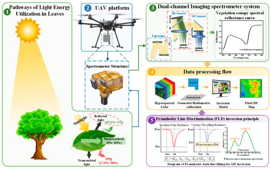
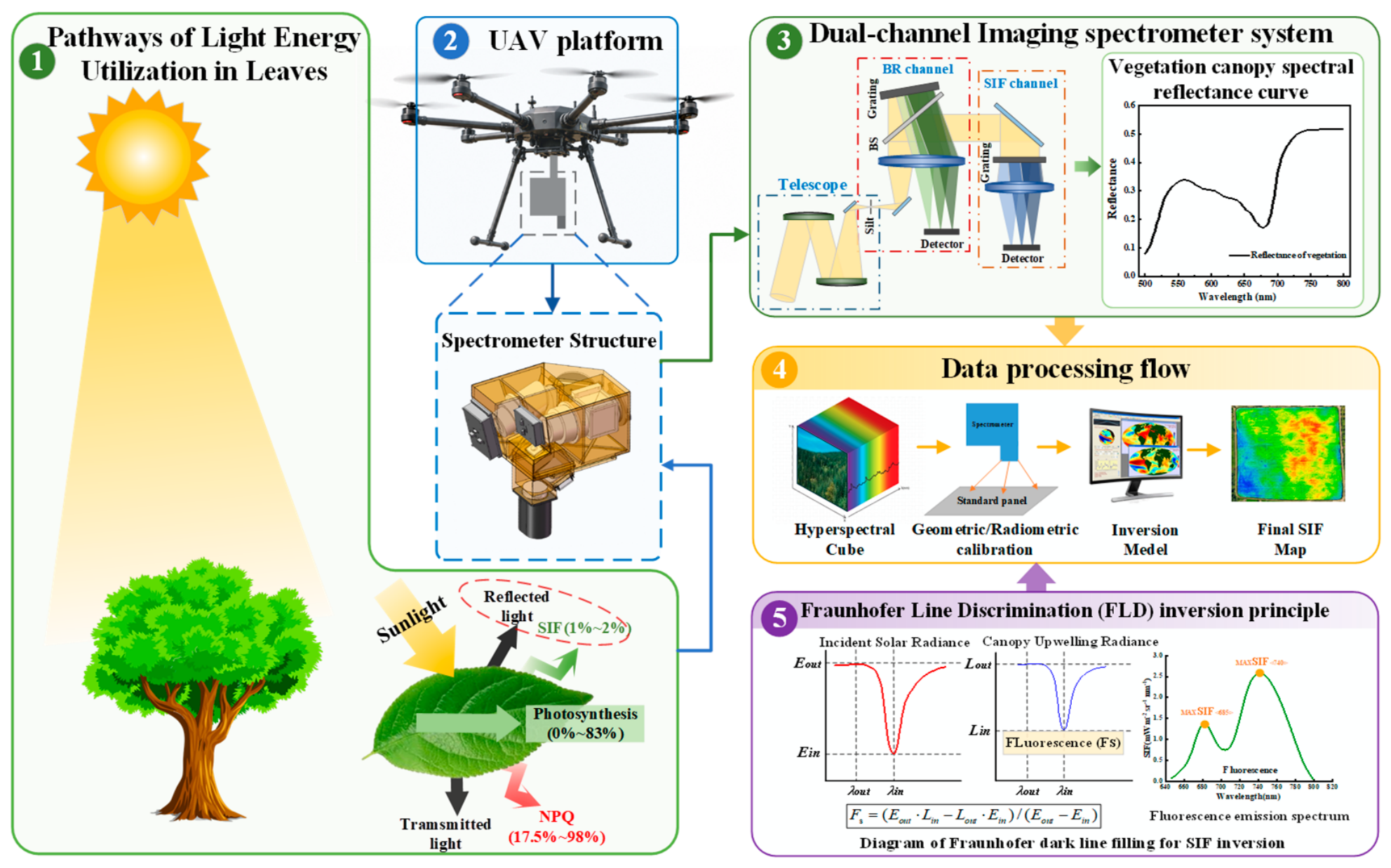
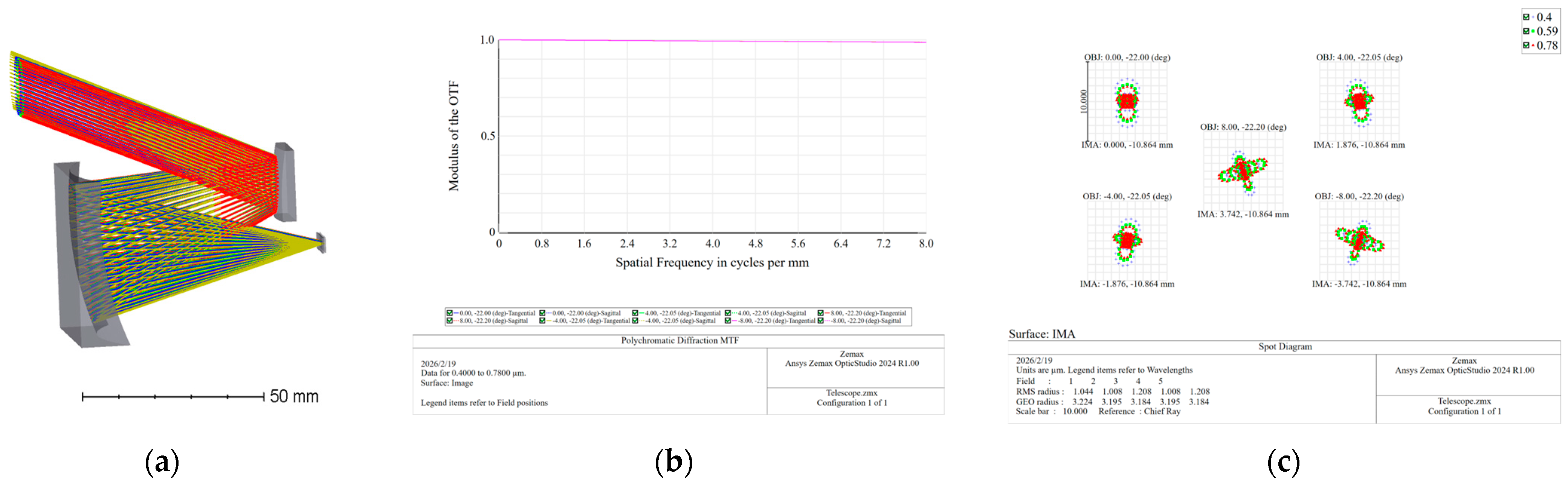
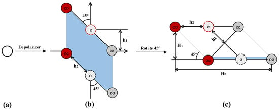
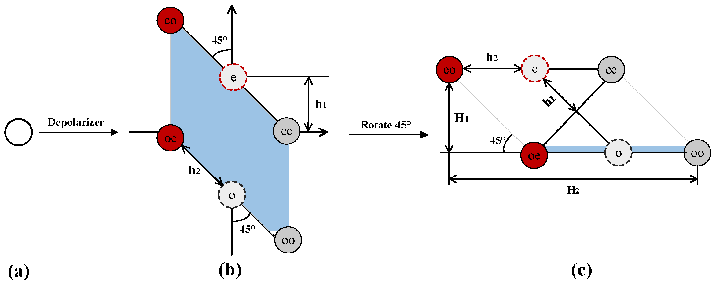
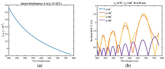
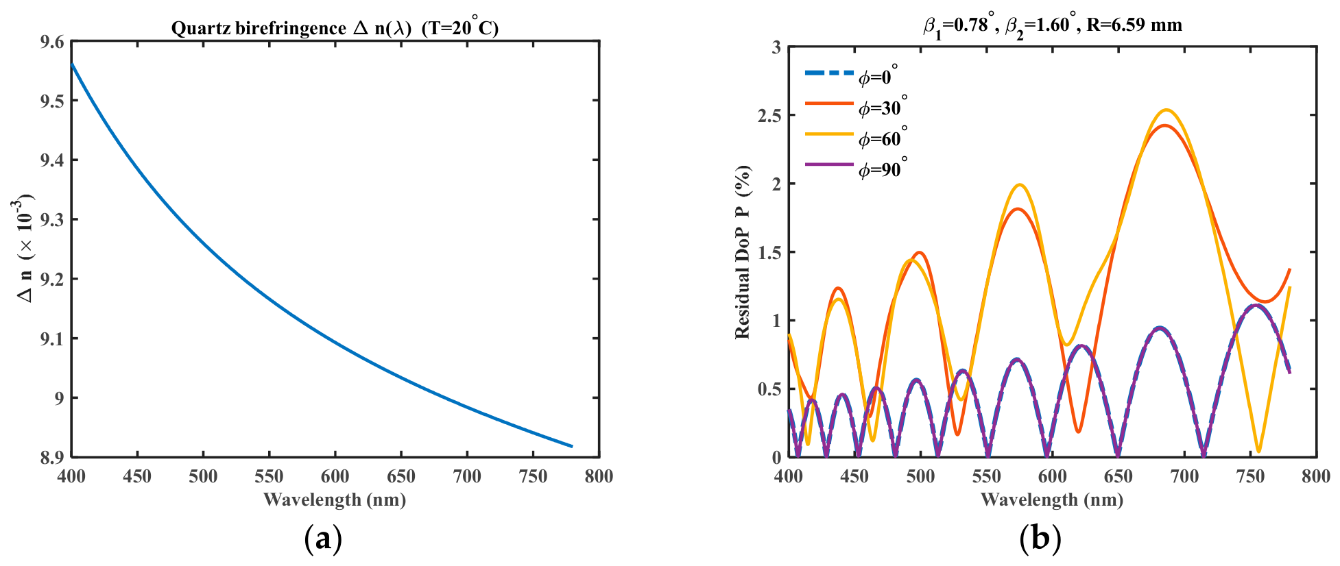
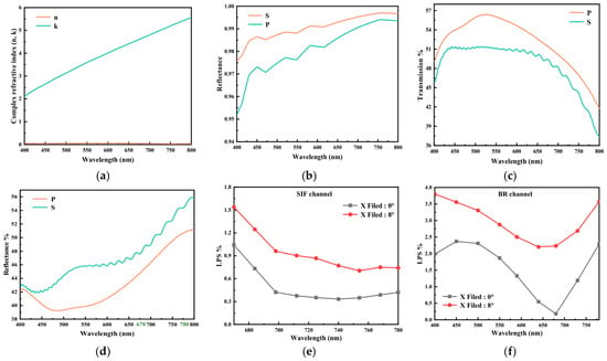
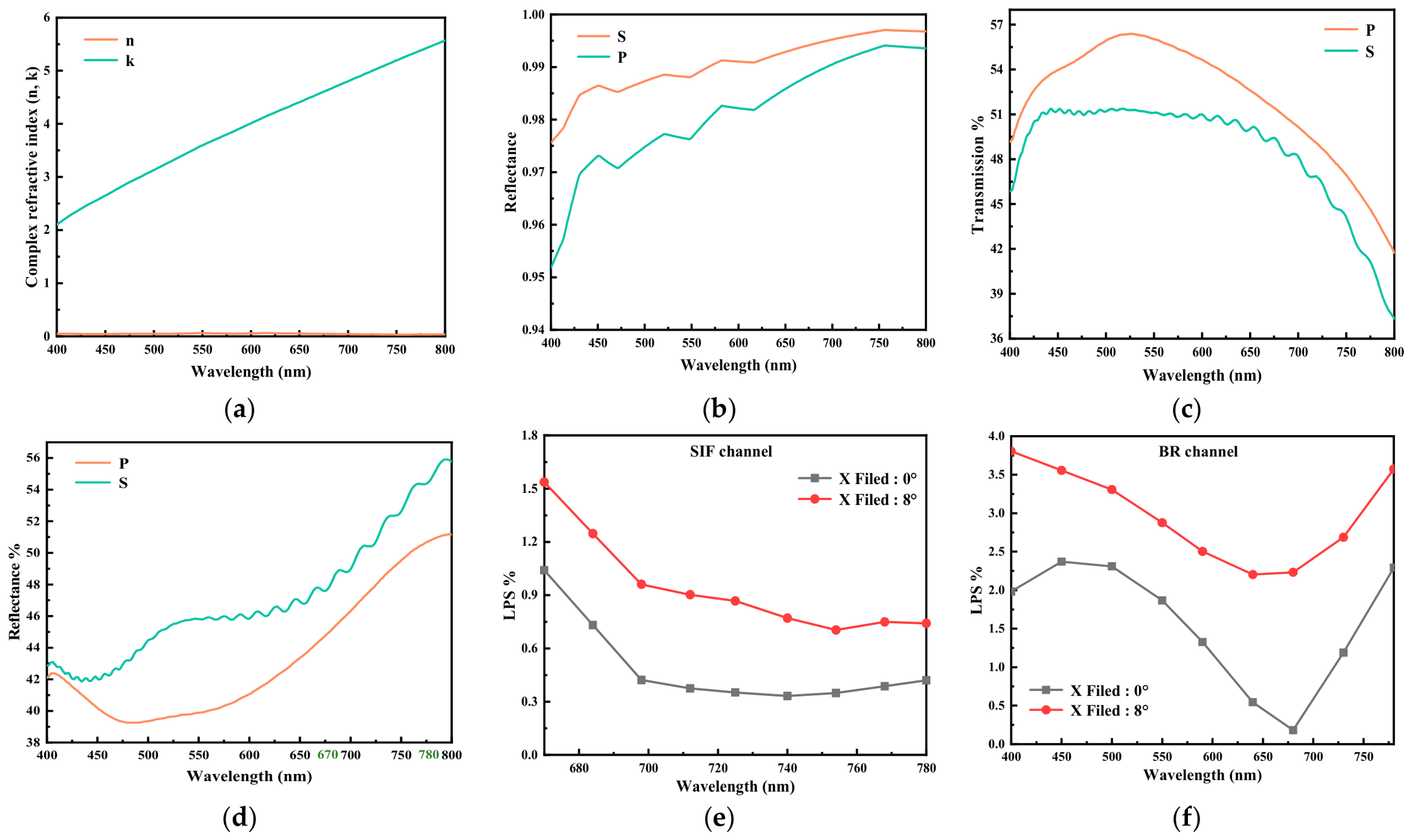
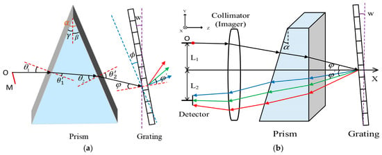
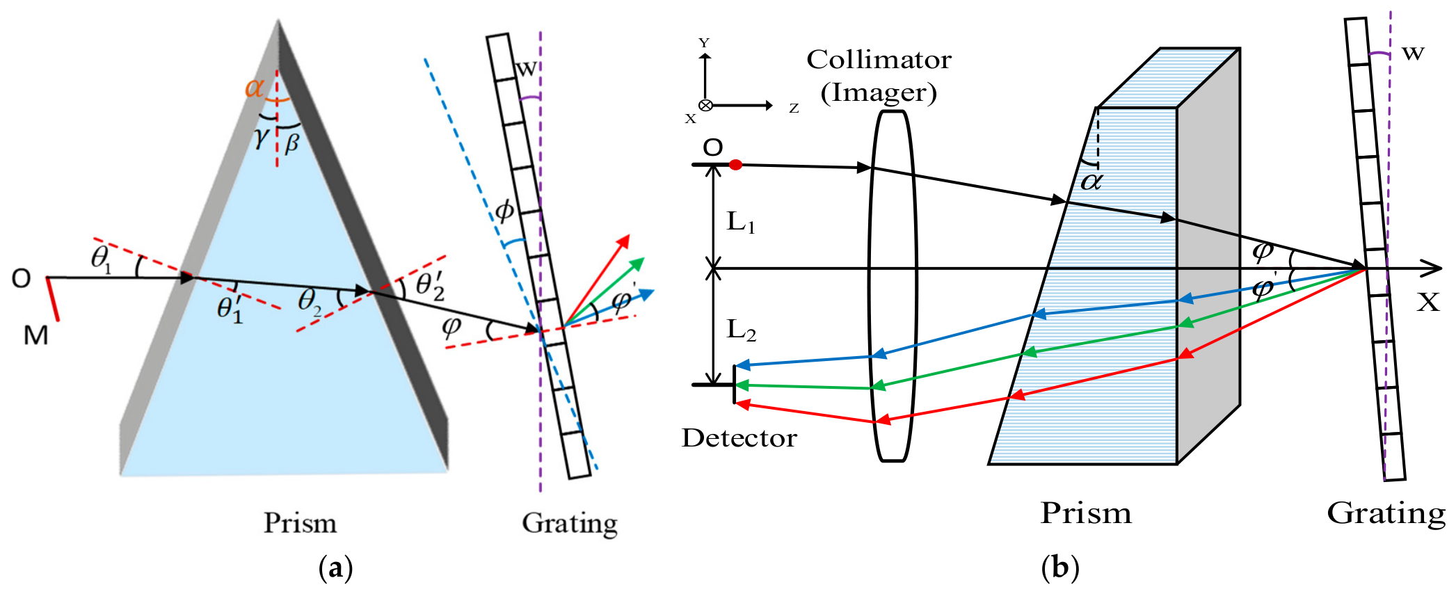
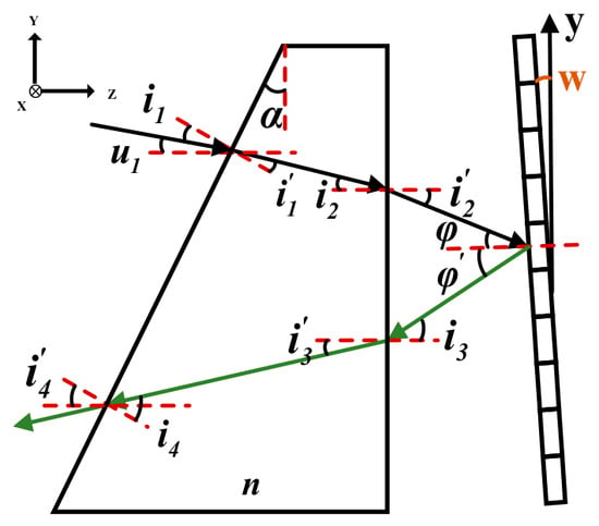
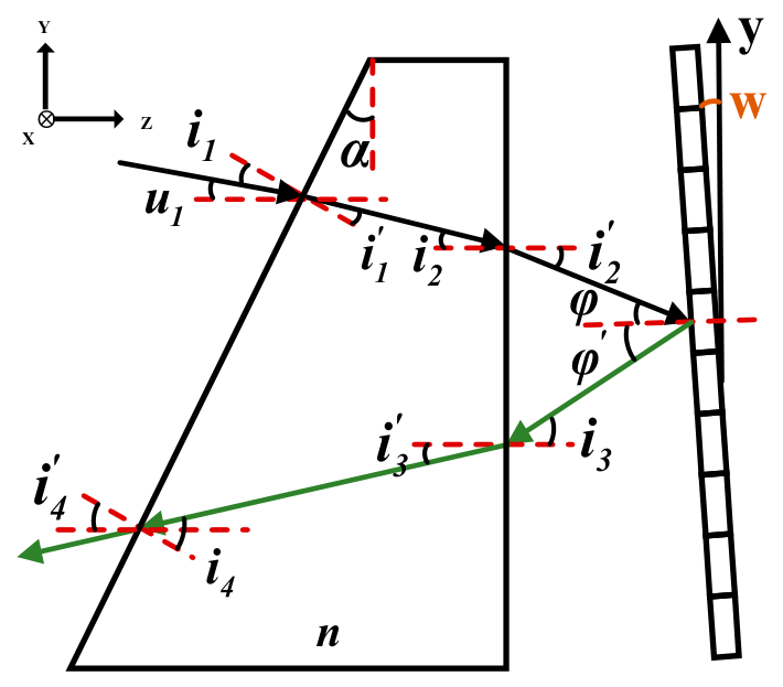
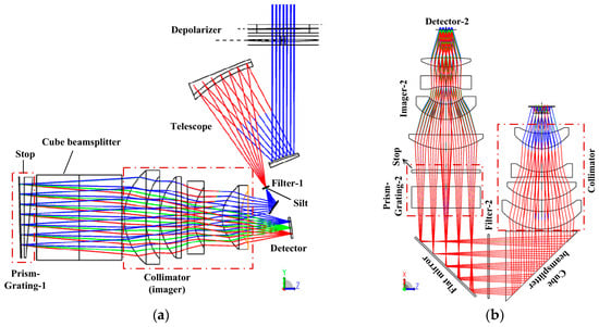
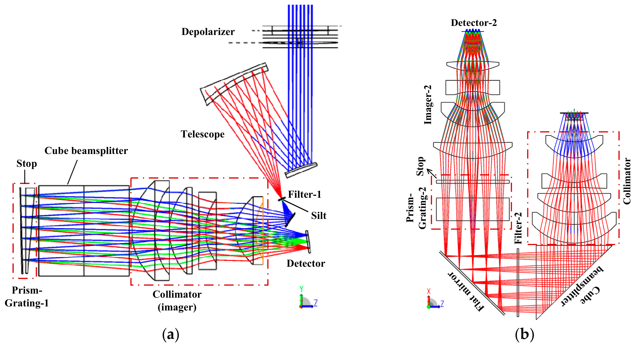
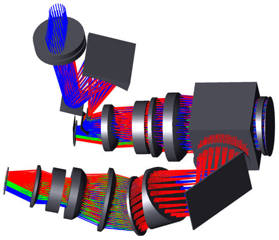
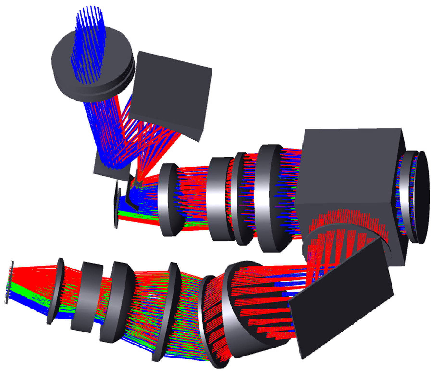
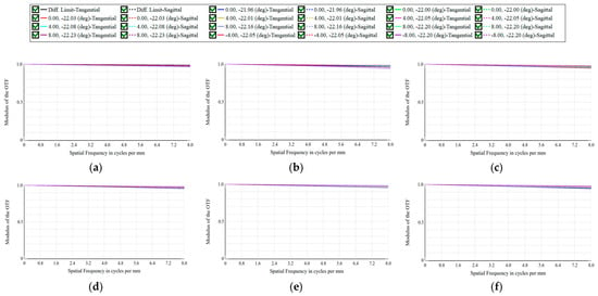
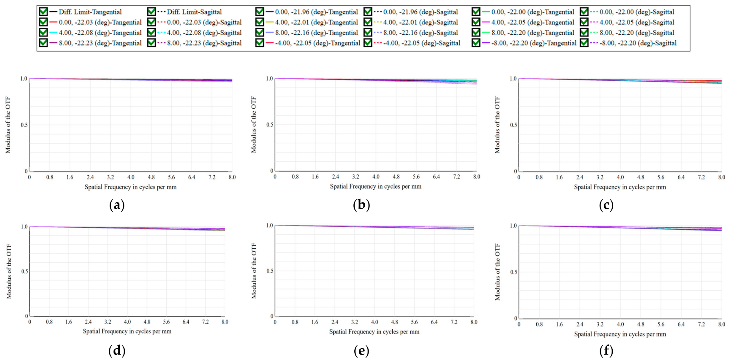
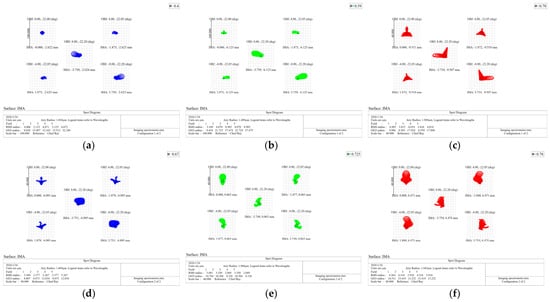
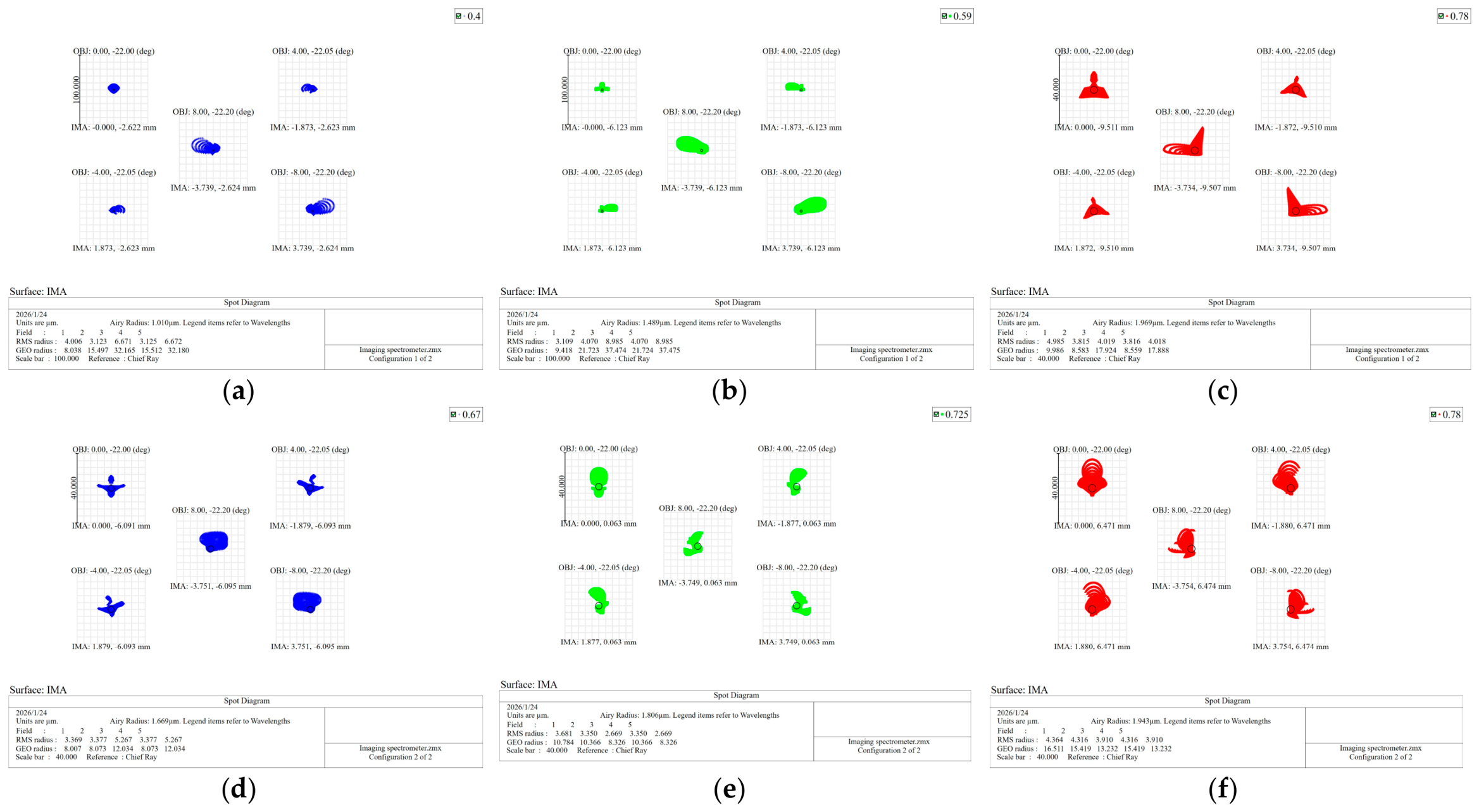
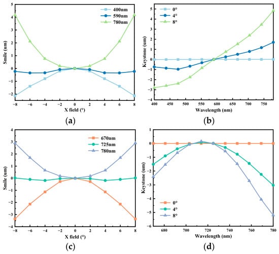
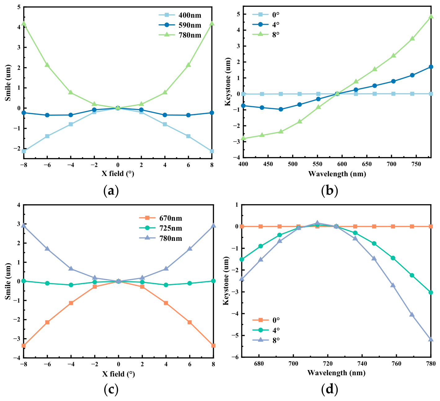
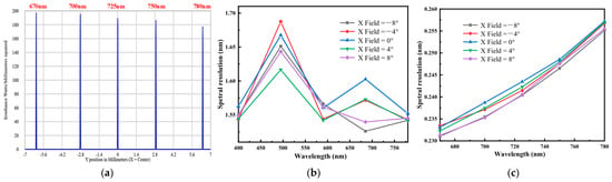
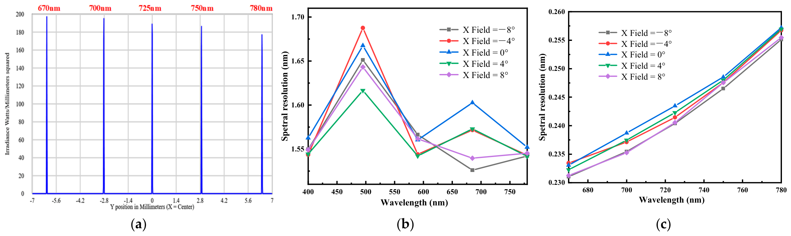
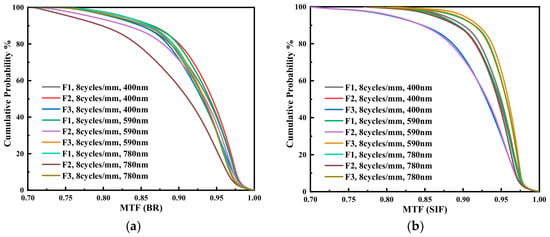
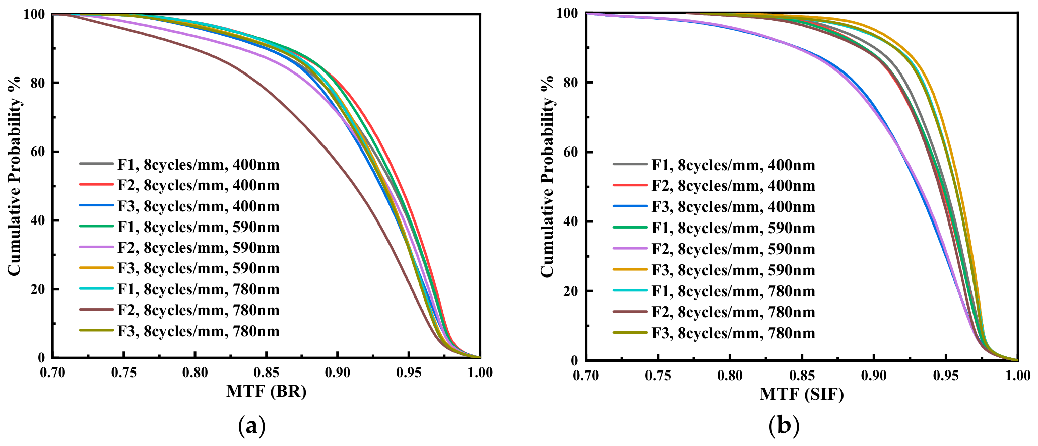
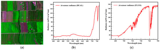
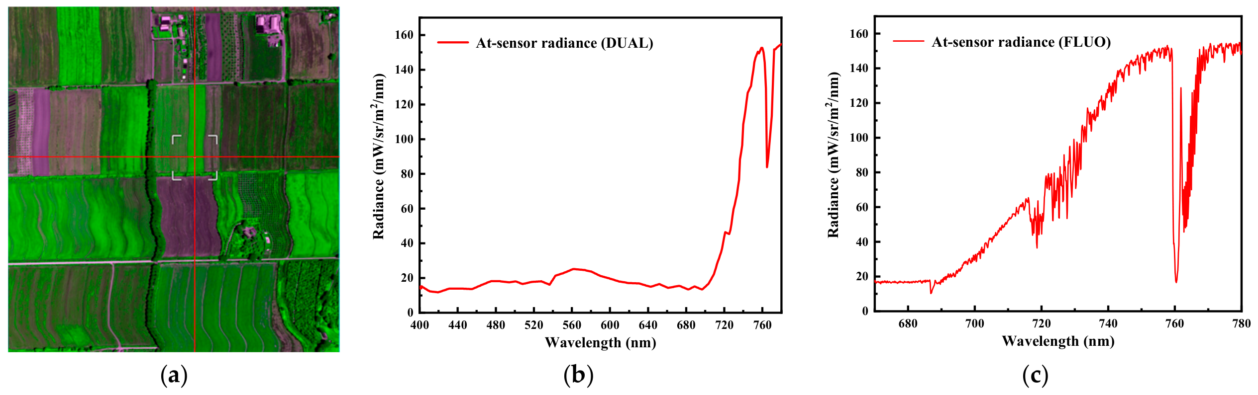
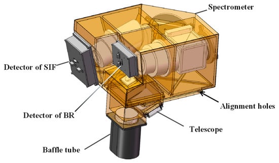
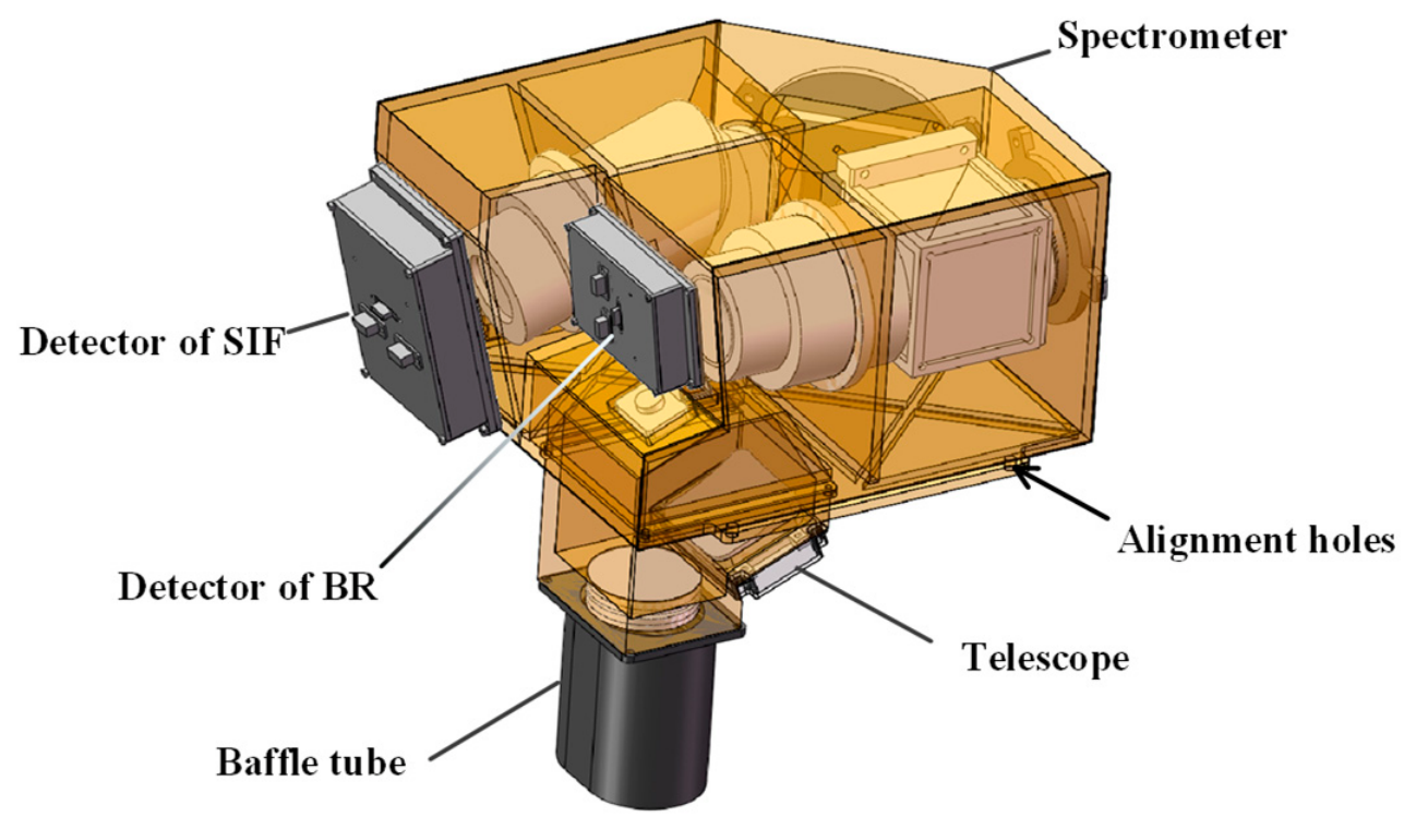
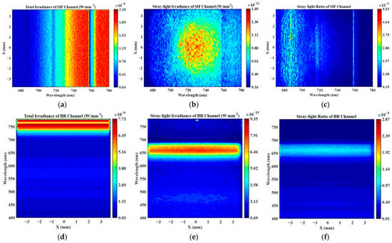
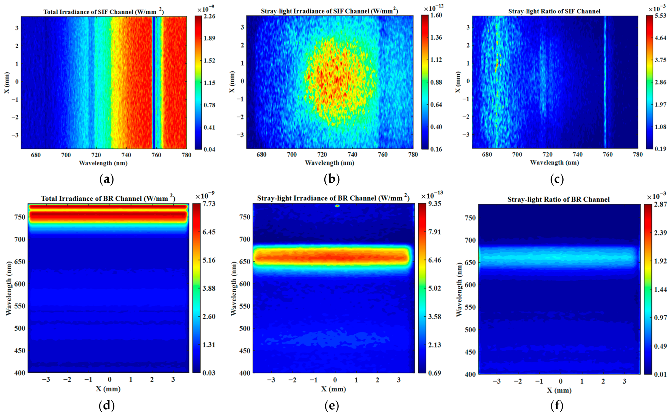
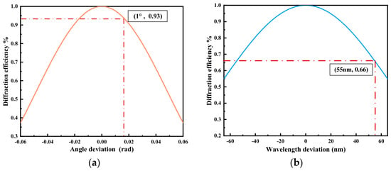
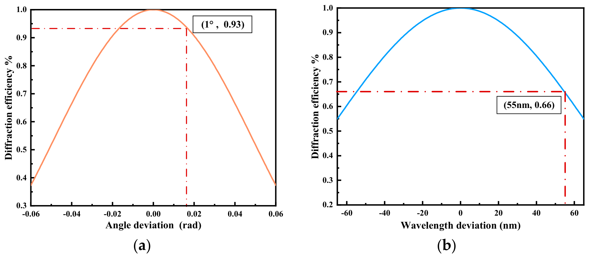
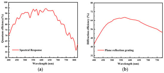
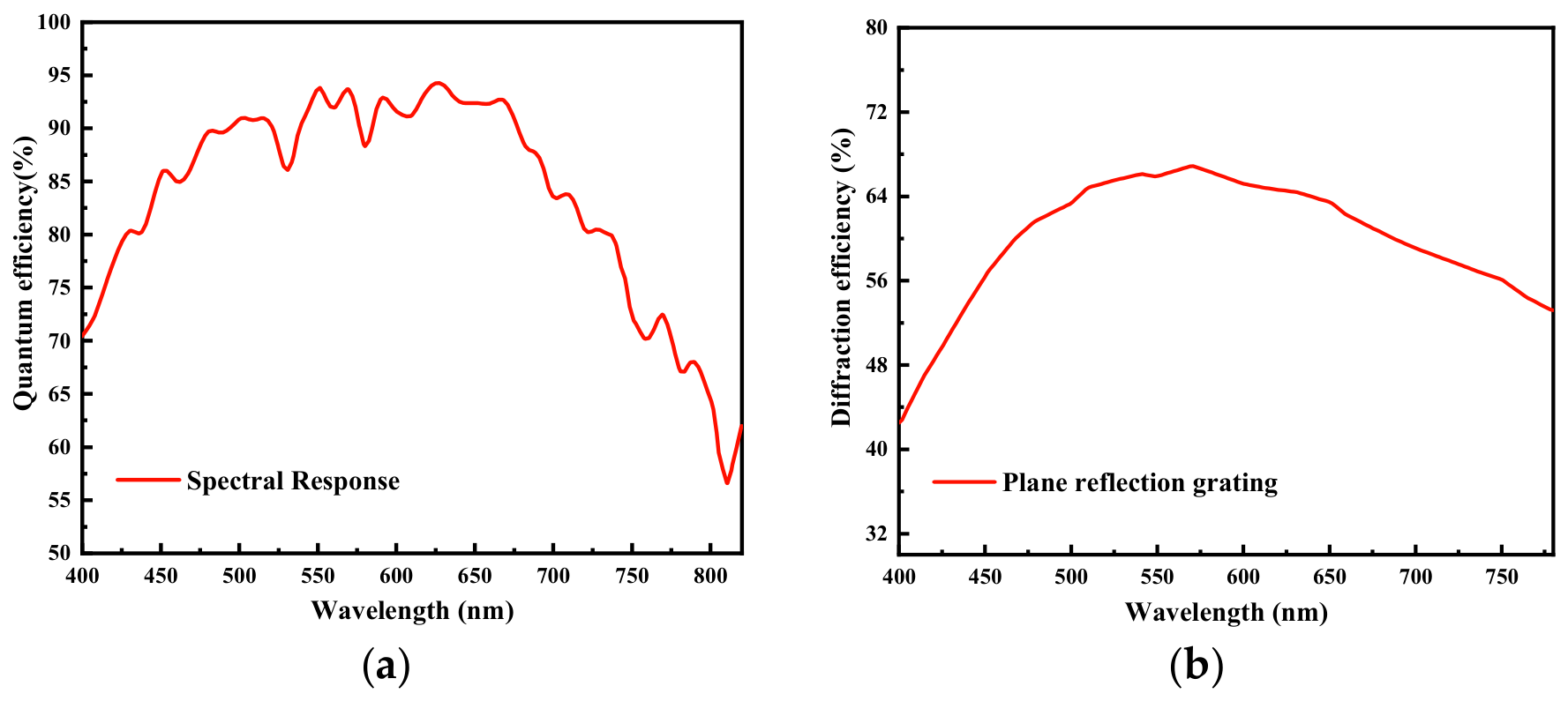
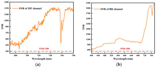
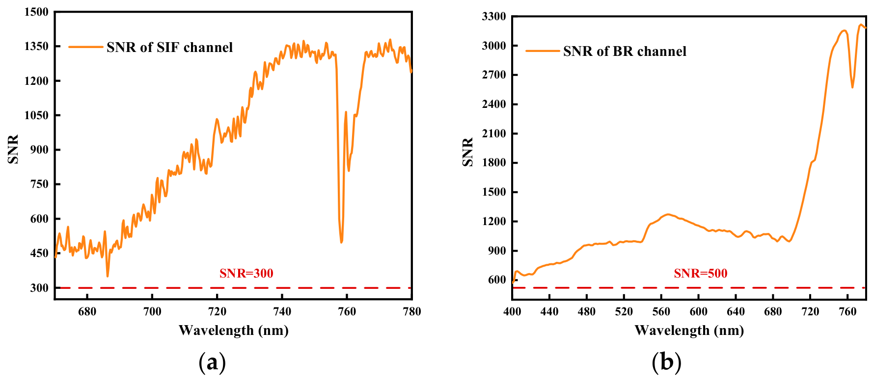
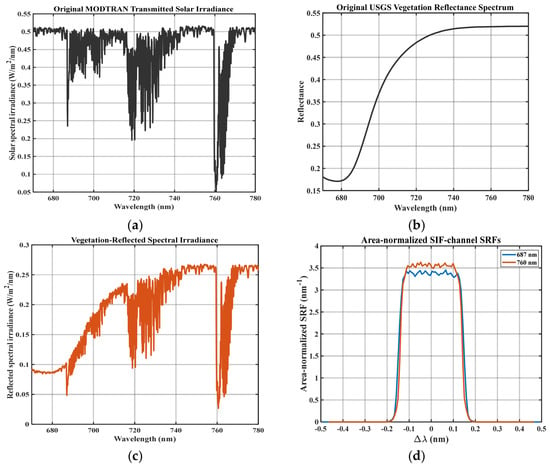
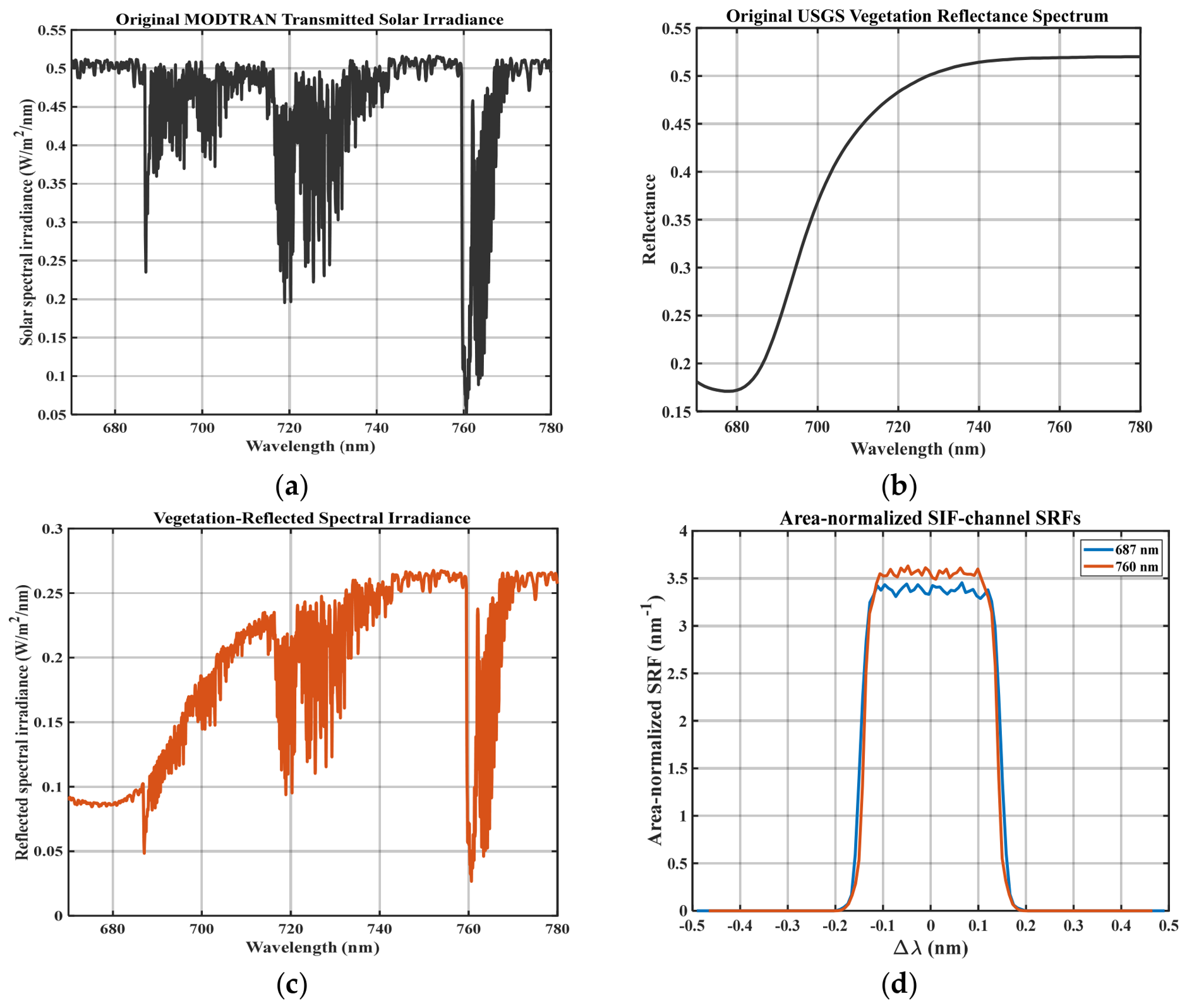
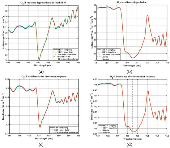
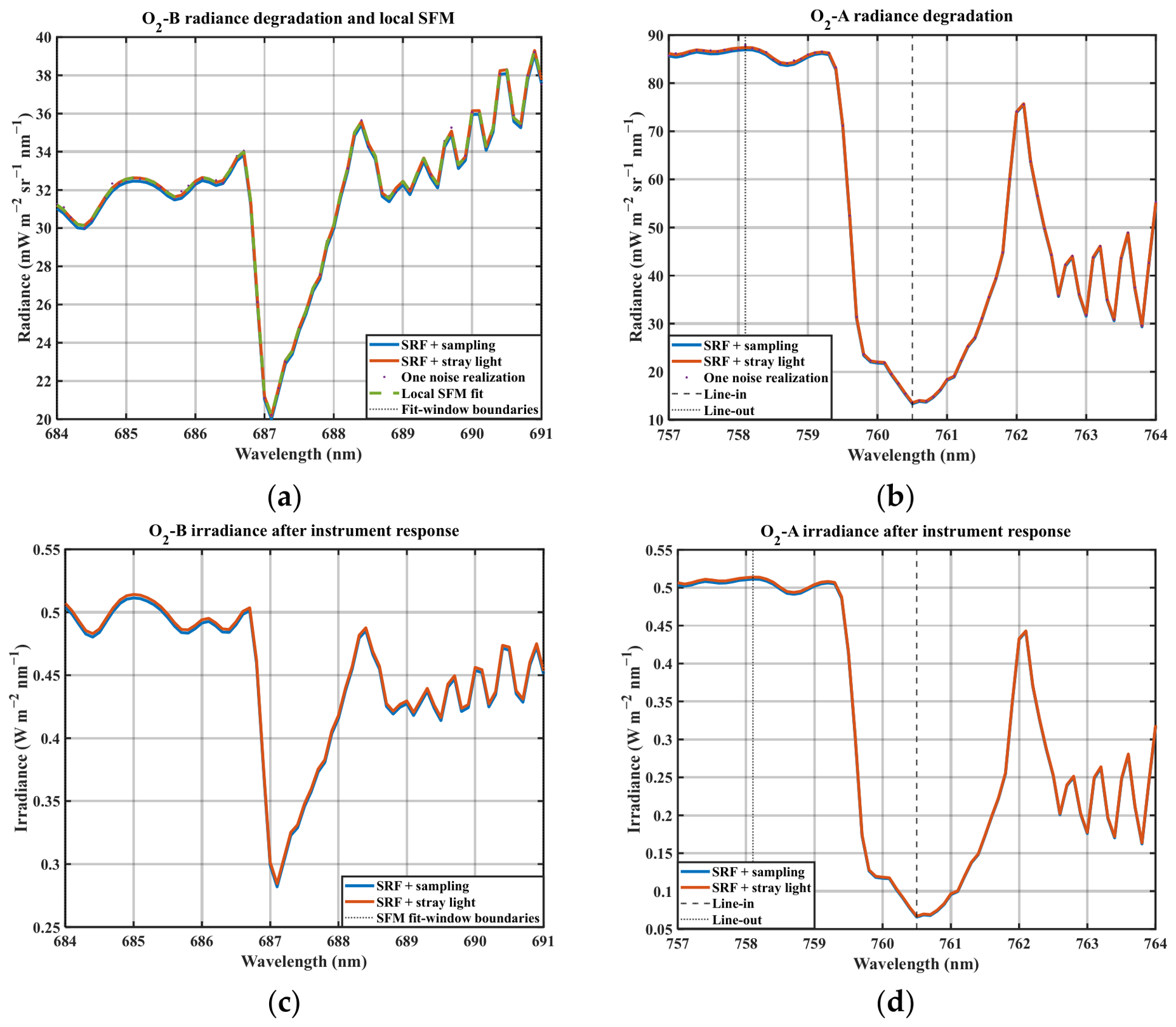

Disclaimer/Publisher’s Note: The statements, opinions and data contained in all publications are solely those of the individual author(s) and contributor(s) and not of MDPI and/or the editor(s). MDPI and/or the editor(s) disclaim responsibility for any injury to people or property resulting from any ideas, methods, instructions or products referred to in the content. |
© 2026 by the authors. Licensee MDPI, Basel, Switzerland. This article is an open access article distributed under the terms and conditions of the Creative Commons Attribution (CC BY) license.