


Highlights
What are the main findings?
- Development of a near-real-time and fully automated processing for the detection and monitoring of extreme atmospheric events based on IASI spectra.
- Implementation of a PCA-based algorithm (IASI-PCA) systematically detecting fires, volcanic eruptions, dust plumes, pollution events, and other extreme events.
What are the implications of the main findings?
- Supports long-term processing of global datasets, scientific analysis of extreme atmospheric events, and near-real-time monitoring for risk management.
- Provides a reproducible framework, applicable to other atmospheric sounding satellite missions, allowing consistent detection via multi-instrument synergy.
Abstract
Extreme atmospheric events are rare phenomena characterized by unusual intensity or chemical composition compared to the atmospheric background state. Many such events, in the context of global warming, pose threats to human health, thereby making their early detection and monitoring essential. The Infrared Atmospheric Sounding Interferometer (IASI), able to measure more than 30 atmospheric chemical species on a global scale, offers strong potential in this context. However, the large volume of current and upcoming satellite observations makes intelligent data screening more and more challenging. This work aims to overcome this limitation by developing a dedicated algorithm based on Principal Component Analysis (PCA) of Level 1C IASI spectra. Named IASI-PCA, it is designed for the systematic detection of fires, volcanic eruptions, dust storms, pollution plumes, and other extreme atmospheric events that remain unclassified. The detected events are defined as spectral outliers relative to the representative global variability of IASI observations under normal or unperturbed conditions. The detection of an individual spectrum is driven by its anomalous behavior in selected spectral domains, where a set of optimized indicators corresponding to more than 10 species has been defined to discriminate events according to their chemical signatures. This methodology has been implemented in a near-real-time operational system providing detection and classification products within one hour and one day, respectively. The IASI-PCA approach has been applied to multiple case studies demonstrating that it is a powerful tool for: (1) efficiently detecting and monitoring fires, whether isolated sources or extended plumes; (2) handling both clear and cloudy conditions; (3) detecting dust plumes predominantly associated with calcite; (4) identifying pollution sources; and (5) detecting volcanic events. The consistency of our results with those obtained with the EUMETSAT Principal Component Compression (PCC) is also illustrated through the processing of a representative study period.
1. Introduction
Due to climate change, an intensification and an increasing frequency of extreme events such as wildfires, heat waves, and anthropogenic pollution episodes have been observed in recent decades (e.g., [1,2,3]). These episodic events, along with dust storms and volcanic eruptions, significantly perturb atmospheric composition at global and regional scales, with impacts on air quality, climate, ecosystems, and human health. The need for rapid detection and monitoring of such events has therefore become increasingly critical, for both risk management through near-real-time data processing, and air quality surveillance and forecasting.
Spaceborne hyperspectral infrared sounders such as the Infrared Atmospheric Sounding Interferometer (IASI [4]) constitute a valuable contributor to the global monitoring of atmospheric composition, by collecting more than one million measurements every 24 h (day and night) around the globe and giving access to the spatial structures and temporal evolution of trace gas concentrations. With two IASI sensors currently in orbit on board MetOp-B and MetOp-C, allowing the observation of many regions of the Earth more than once per day, IASI has great potential for the early detection and monitoring of extreme atmospheric events, although it was initially designed to support Numerical Weather Prediction (NWP) centers by retrieving meteorological parameters such as temperature and moisture profiles. However, the main challenge arises from the large amount of data to be processed, and the full potential of IASI for monitoring extreme events is still far from being fully exploited.
Given the large volume of existing and forthcoming datasets, the development of automatic detection tools offers a promising perspective for efficiently targeting and extracting relevant information. In this paper, we investigate the application of Principal Component Analysis (PCA) on atmospheric spectra for detecting extreme events, defined as data outliers relative to the natural variability of the atmosphere. The PCA technique has been widely employed as a Principal Component Compression (PCC) technique for hyperspectral infrared observations [5,6] since it not only allows efficient extraction of the pertinent spectral information but also reduces the random instrumental noise. This approach has been operationally implemented in the framework of data dissemination [7], with the aim of significantly reducing data volume with almost no loss of atmospheric information [8,9].
In contrast, the present study uses PCA by taking advantage of its ability to target reconstruction anomalies arising from unusual spectral features in the original radiances, which can be associated with rare or extreme events. Using IASI measurements, ref. [10] demonstrated that PCA-reconstructed radiances preserve the relevant signal associated with atmospheric trace gases, therefore confirming their suitability for retrieval purposes. Rather than retrieving trace gas concentrations by a standard but time-consuming retrieval algorithm, the objective of this work is to detect quickly anomalous spectral signatures associated with particular species. We focus on a set of trace gases and one carbonate mineral that are both well observed by IASI [11] and strongly linked to extreme atmospheric events, listed hereafter.
- -
- Carbon monoxide (CO). CO is a recognized indicator of biomass burning emissions, which has been extensively observed by IASI since the early mission phase (e.g., [12,13,14]). It has a relatively long lifetime (around 2 months), making it also a good tracer of long-distance fire transport and anthropogenic pollution.
- -
- Carbon dioxide (CO2). Despite its large background concentration, CO2 exhibits detectable short-term variability in the thermal infrared during intense emission events such as wildfires (e.g., [15]).
- -
- Volatile organic compounds (VOCs), including acetylene (C2H2), ethylene (C2H4), methanol (CH3OH), formic acid (HCOOH), and hydrogen cyanide (HCN). They are all well-known tracers of biomass burning with relatively short lifetimes, ranging from a few hours for C2H4 [16], several days for HCOOH [17], and CH3OH [18] to several weeks for C2H2 [19], except for HCN, which has a lifetime of 2–4 months [20]. They have been repeatedly detected in IASI observations of wildfire plumes (e.g., [18,21,22,23]).
- -
- Ammonia (NH3). It is a short-lived species (a few hours, [18]), emitted by agricultural activities, biomass burning, and industrial sources [24]; it presents strong infrared absorption features and has been widely studied using IASI measurements (e.g., [25,26]).
- -
- Sulfur dioxide (SO2). SO2 is generally used as a tracer of volcanic emissions [27,28].
- -
- Calcium carbonate or calcite (CaCO3). Mineral aerosols originate from wind erosion processes in arid and semiarid lands. Once uplifted into the atmosphere, calcite can play a role in climate change, which explains the growing interest in recent years [29,30].
The robustness of the PCA-based detection method has already been successfully demonstrated [31]. In this paper, we provide the methodological framework and illustrate its capabilities through a series of diverse application cases. This paper is organized as follows. In Section 2, we concisely present the IASI instrument and data. The methodology adopted is detailed in Section 3. Section 4 provides examples of applications. Section 5 presents the discussion and perspectives of the approach, and Section 6 summarizes our results and conclusions.
2. IASI Data
Developed by CNES (Centre National d’Etudes Spatiales, France) and operated by EUMETSAT (European Organization for the Exploitation of Meteorological Satellites, Germany), the IASI instrument is a Michelson-type Fourier transform spectrometer, coupled with an Integrated Imaging System (IIS) and designed to measure the atmospheric infrared radiation emitted by the Earth atmosphere/surface system. The main characteristics of the instrument are summarized in Table 1.
Table 1.
IASI main characteristics.
The IASI instruments are part of the EUMETSAT Polar System (EPS) program, which consists of a series of three MetOp satellites—MetOp-A, MetOp-B and MetOp-C platforms—launched in 2006, 2012 and 2018, respectively, by the European Space Agency (ESA) and EUMETSAT. MetOp-A was deorbited in 2021. With 14 polar sun-synchronous orbits per day, each instrument provides global observations twice a day (day and night) over a swath width of km on both sides of the sub-satellite track, with a local overpass time at 09:30 AM and PM. IASI is a cross-track scanning instrument, with a total of 30 fields of regard (FOR) per scan. Each FOR projects onto the ground an area of km at nadir and is composed of circular pixels, known as instantaneous fields of view (IFOVs). Each IFOV corresponds to a 12 km diameter footprint on the ground at nadir. IASI L1C spectra cover a range extending from 645 to 2760 cm−1, with a sampling step of 0.25 cm−1 and a spectral resolution of 0.50 cm−1 (apodised), resulting in 8461 spectral channels for every single spectrum. The full spectral range is divided into three spectral bands defined as follows: 645–1210 cm−1, 1210–2000 cm−1, 2000–2760 cm−1, respectively, for band 1, band 2 and band 3. In this analysis, we use level 1C (L1C) products (spectra and associated time and geolocation) that have been acquired by the IASI instrument on MetOp-A, MetOp-B and MetOp-C, and stored in BUFR format on the SPIRIT/IPSL cluster. Each file consists of one granule containing 3 min of data, which corresponds to 22 or 23 IASI scan lines. Therefore, every BUFR file counts 2640 or 2760 spectra.
3. IASI-PCA Methodology for Detecting Exceptional Atmospheric Events
In this section, we present the methodology developed for detecting extreme atmospheric events using IASI L1C spectra. We first outline the general detection framework, then introduce the concept of spectral indicators designed for automatic and spectrally targeted detection. We finally provide a detailed description of the Principal Component Analysis applied to extract relevant signal components.
3.1. Principle of Extreme Event Detection
The approach relies on analyzing the variability of a representative set of radiance spectra encompassing all geophysical conditions. As noted by Ref. [8], it is common to use radiances rather than brightness temperatures to perform PCA, not only because the instrumental noise is more uniform in radiance dimensions, but also because negative radiances (existing on several occasions) would prevent conversion to brightness temperature in spectral regions with low signal-to-noise ratio. The PCA technique (detailed in Section 3.3) exploits correlated spectral features to derive the main eigenvectors and eigenvalues that characterize the natural atmospheric variability. Through data compression and reconstruction, the method effectively separates the spectrally correlated atmospheric signal—captured by the leading principal components—from the uncorrelated spectral noise, which is distributed among the less significant components. Reconstruction anomalies, corresponding to unusual spectral features, are identified as outliers and are associated with rare or extreme atmospheric events.
The detection of outliers is based on the analysis of the normalized spectral residual defined as the difference between the original spectrum and the reconstructed one , normalized by the IASI noise covariance matrix :
From this residual, a reconstruction score corresponding to the standard deviation stdv of the spectral residual with respect to the mean level <r> = mean, estimated over a given spectral domain is computed to efficiently highlight reconstruction anomalies:
Since the residual is normalized by the IASI noise (see Section 3.3.1 for details), the reconstruction score is expected to be close to unity if the original radiances are well fitted by the reconstructed ones. On the contrary, a significant deviation from unity suggests that the current spectrum contains features that are not well represented in the statistics of the reference basis, which is precisely the signature of interest.
3.2. Detection of Reconstruction Anomalies Using Indicators
To spectrally target reconstruction anomalies, reconstruction scores are computed over reduced and carefully selected spectral domains associated with species or geophysical parameters. These spectral domains, hereafter referred to as “indicators”, have been selected for their sensitivity to the target species and geophysical parameters in the IASI measurements and further refined based on atmospheric spectroscopy expertise and sensitivity analysis. This method allows automatic detection and multi-species monitoring by identifying narrow emission or absorption features in the spectra. A total of 30 indicators are specified, including 11 species and 4 geophysical parameters. By defining such a comprehensive set of indicators, the IASI-PCA method can capture various types of events, including fires, volcanic eruptions, desert dust plumes, pollution events, and possibly other unknown events. Examples of thematic applications are provided in Section 4.
As illustrated in Table 2, each indicator is defined by:
- Its spectral domain , where the wavenumbers correspond to the exact spectral samples provided in the L1C spectra;
- Its name, given by the species or the parameter associated with the spectral domain;
- Its reconstruction score noted corresponding either to the standard deviation (noted ) or the mean (noted mean) of the spectral residual, calculated over the corresponding spectral domain;
- Its diagnostic, denoted “diagn”, allows the analysis of the residual to be supplemented and corresponds either to the mean or to the stdv of the spectral residual computed over the corresponding domain;
- Its detection thresholds, specific to day and night situations, allow the automatic detection of outliers. These thresholds are instrument-specific since each IASI instrument exhibits distinct noise properties.
Table 2.
List of indicators used to detect extreme events and for which reconstruction scores are computed over reduced spectral intervals targeted on species or parameters of interest. They have been defined by using known absorption features [32,33]. A detection occurs when the score associated with at least one indicator exceeds the threshold. As an example, day and night thresholds corresponding to the case of IASI-C are given.
It is emphasized that indicators are defined by their spectral domain, and not necessarily the species from which they take their name, as these domains may include contributions from other interfering species. Any spectrum showing a reconstruction score higher than the detection threshold is considered an outlier. By construction, the method allows the detection of spectral features that deviate from the natural variability of the atmosphere. Due to the complexity of spectrally correlated statistics of IR spectra, detection of an outlier does not systematically correspond to an anomalous concentration of the associated gas. It is the spatial consistency, associated with the simultaneous detection involving several indicators, which allow to discard false positives. Further techniques, in addition to the high reconstruction scores, are therefore required to identify and characterize the detected anomaly (see Section 3.4).
For each IASI model, the adjustment of the day and night detection thresholds is based on the IASI-PCA processing of January 2021, a period chosen because it was relatively free of extreme events (no anomalous signal was detected in the scores over this period) and because it represents a sufficiently large statistical sample. Details on these statistical samples can be found in Appendix A. Reconstruction scores associated with all indicators are computed for each day at a global scale. The resulting score distributions are then analyzed for each indicator and IASI IFOV, separating day and night. Examples of such distributions are provided in Appendix A. Most indicator distributions are non-Gaussian and are generally better fitted by a log-normal distribution, although some, such as Surf_n indicators, appear closer to Gaussian. However, their second moment or standard deviation remains well defined, and day and night thresholds are determined according to the following formula:
Any score value exceeding this threshold is considered an outlier.
In a first step, is a tolerance factor set to , and as for any threshold, this value is somewhat arbitrary. Its sensitivity to the exact number of retained outliers is not critical for the objective of the study, i.e., for detecting and analyzing anomalous spatial distributions of high scores (often associated with plumes of atmospheric constituents). These preliminary thresholds are used to identify and remove outlier spectra from the reference datasets (approximately 5% of reference spectra are discarded for each IASI model). This enhances the capability of IASI-PCA to efficiently detect unexpected events and ensures that anomalous spectra, excluded from the training sets, are by construction less accurately reconstructed and thus more easily detected as outliers. These cleaned reference datasets form the new, final training sets from which a final PCA basis is generated.
Second, a final threshold estimation is performed using this clean basis, again processing January 2021. The resulting score distributions are used to compute final detection thresholds according to Equation (3). The final tolerance factor used for each indicator is determined empirically to limit false detections while retaining known extreme events. This yields a default tolerance factor of 5.5 for all IASI models, with a lower tolerance of 4.5 and 5.0 for a subset of indicators. The full table of retained tolerance factors is given in Appendix A.
As a final remark, since the normalization properly accounts for the noise covariance matrix of each of the four IASI IFOVs, the use of a single day/night detection threshold for all four pixels of a given IASI instrument is justified. This threshold corresponds to the threshold average computed over the four IFOVs’ values.
3.3. Principal Component Analysis Applied to IASI Spectra
3.3.1. Band Separation, Interbands, Reference Datasets, and Noise Normalization
Prior to performing PCA, it is essential to clearly define the methodological settings for preparing the data, including the treatment of IASI bands, the choice of reference datasets, and the choice of the normalization matrix.
In line with the EUMETSAT compression approach [34], the three IASI spectral bands Bj (with ) are considered separately, reflecting differences in detector characteristics and noise properties across bands. Examination with and without band separation of the eigenvalues showed significant interband differences, thereby supporting independent treatment. The three bands are separated as follows:
- B1: [649.0; 1149.5] cm−1, i.e., 2019 spectral samples;
- B2: [1225.0; 1934.5] cm−1, i.e., 2839 spectral samples;
- B3: [2025.0; 2760.0] cm−1, i.e., 2941 spectral samples.
Unlike Table 1, which presents the nominal IASI instrument spectral bands, these intervals are specifically defined for the PCA processing. In particular, the interband regions are not considered, as mentioned later and detailed in Appendix B.1.
This choice is further justified, as it allows the compression of bands B1 and B2 independently, even when the quality of band B3 is degraded.
In the IASI interband regions (see the exact limits below), measurement noise increases due to reduced optical transmission and detector sensitivity, as pointed out in Ref. [35]. Some irregularities are observed, including rapidly varying noise levels, decreased measurement quality at band edges, and discontinuities introduced by the band-merging process. This is because three spectral bands having different instrument response functions (ISRF) are merged to generate the L1C spectra on a fixed spectral grid with a fixed almost Gaussian ISRF. In addition, coding tables used for data transmission on the ground may change characteristics of the noise when crossing from one band to another. We therefore choose to exclude the two IASI interbands defined below:
- B1/B2: [1149.75; 1224.75] cm−1;
- B2/B3: [1934.75; 2024.75] cm−1.
We note that these spectral intervals are slightly different than those defined in Ref. [35]. Further details and justifications for this methodological choice can be found in Appendix B.1.
For each IASI instrument, PCA is performed with differentiated reference datasets of IASI Level 1C spectra, corresponding to the 4 IFOVs and 3 IASI bands noted Bj with . The goal of the reference datasets optimization is to ensure that they reflect typical atmospheric conditions rather than rare anomalies. Not only must the training set be as free as possible from extreme events, but also be representative of the full range of latitudes, seasons, weather and solar illumination conditions, cloud cover, viewing angles and surface types. Using a large dataset improves the separation of signal and noise, reduces non-representative correlations, and limits the over-representation of specific conditions [8,36,37]. It is recommended to use a number of spectra , where is the spectral sample size. In the case of IASI, where , a training set comprising a few thousand spectra [8] or approximately 70,000 spectra [37] are considered appropriate. In our case, we therefore choose to build reference datasets of approximately 120,000 spectra (with an equal distribution of daytime and nighttime observations), randomly distributed on a global scale over one year (for consistency, 2020 was chosen, as the three IASI instruments were operational at that time). The resulting datasets are balanced with respect to illumination conditions (approximately 50% spectra during day and 50% spectra during night) and cloud coverage, with about 40% overcast spectra, 40% mixed, and 20% clear sky cases. Table 3 gives an example of the percentage of daytime acquisitions and the corresponding fraction of spectra falling into each cloud category for IASI-A.
Table 3.
Total number of IASI-A spectra for each IFOV and percentage of daytime, clear-sky (cloud fraction of 0%), mixed (cloud fraction between 1 and 99%), and overcast (cloud fraction of 100%) spectra.
In addition, only spectra for which the IASI general quality flag (GQisFlagQual: The flag is TRUE (1) if an anomaly was detected in IASI Level 0 or Level 1 processing, FALSE (0) otherwise [38]) is not set are retained. Spectra are sampled according to their latitude to prevent over-representation of high latitudes, which are more frequently observed by a polar-orbiting sounder. The following latitudinal sampling scheme has been designed: for a given orbit, 1 spectrum is selected between 75° and 80° latitude (North or South), 2 spectra between 60° and 75°, 3 between 45° and 60°, 4 between 30° and 45°, 5 between 15° and 30° and 6 between 0° and 15°. A well-distributed choice of scan positions and viewing angles is also ensured.
Finally, as discussed in Section 3.2, these reference datasets are cleaned by removing as many outliers as possible, identified through the indicators (see Table 2) introduced in this study. It should be stressed that this procedure involves performing an initial PCA procedure based on the covariance matrix of the initial reference datasets, followed by a second computation of the covariance matrix (and the eigen-structures) once the datasets have been cleaned.
Since PCA inherently seeks the directions of maximum variance (principal components), and because the uncorrelated instrumental noise is not uniformly distributed across the wavenumber domain, noise-dominated regions may bias the analysis. To prevent the principal components from being dominated by instrumental noise rather than atmospheric signal, the spectra are normalized by the IASI noise covariance matrix. The normalization matrix is then written as , where is the noise covariance matrix (NCM) of the IASI Level 1C radiances provided to end-users by CNES. The matrices, specific to each instrument and IASI pixel, were generated using L1C spectra over calibration blackbody targets at the end of summer 2020.
As a first approximation, the use of a limited set of indicators justifies adopting a diagonal matrix as a reasonable and sufficient assumption within the scope of our method. To reduce the estimation noise arising from the limited number of spectra used to compute the matrix (nearly spectra), an adjustment is applied to its main diagonal while preserving the significant spectral features. An illustrative example for IASI-A, IFOV pixel P1, is provided in Appendix B.2. Furthermore, as noted by Ref. [10], using a diagonal noise covariance matrix is reasonable for our purposes, since including off-diagonal elements provides no significant benefit.
3.3.2. PCA
The IASI-PCA method, applied to any IASI input spectrum of dimension channels, is structured around 6 main steps, described hereafter.
- Compilation of reference spectra. Let be the training set of IASI Level 1C radiances noted , with the number of spectral channels and the number of spectra in the dataset. As detailed in the previous section, a separate dataset is built for each IASI platform, pixel, and band, leading to about 120,000 spectra per IFOV and platform.
- Computation of the covariance matrix. The global atmospheric variability is represented by the covariance matrix of each dataset , mean-centered and noise-normalized:where denotes the mean radiance calculated over the spectra of the reference basis , is derived from the main diagonal of the error covariance matrix, and the covariance of vector can be written as .
- Eigen decomposition of the covariance matrix. The eigenvectors are derived from the covariance matrix as follows:where the columns of the matrix are the eigenvectors and is the diagonal matrix of eigenvalues sorted in descending order. The eigenvectors describe the directions capturing the maximum variance, while the eigenvalues quantify the variability associated with each of these eigenvector directions. A distinct eigenvector is thus obtained for each band, pixel, and instrument IASI. As an example, the first eigenvectors derived for the IASI-A training set are given in Appendix C.2.
- Truncation and compression. A critical step in PCA is determining the optimal number of principal components () to use (truncation), as it directly affects the method’s capability to detect outliers. The principal component scores can be written as
For each eigenvector basis, the number of principal components required to reproduce the signal is estimated automatically by examining the slope of the descending eigenvalues curves, indicating the transition from signal-dominated to noise-dominated components, as described in Appendix C.1.
- Reconstruction. From the previous equation, an approximation of can be reconstructed:
The resulting reconstructed radiance exhibits a significantly increased signal-to-noise ratio.
- Computation of the normalized spectral residual. The normalized spectral residual is then calculated by taking the difference between the original and reconstructed radiance, as mentioned previously:
The separation of the three IASI bands involves generating three spectral residuals, which are then concatenated to cover the entire IASI spectral range, excluding interband regions where no residual is computed.
- Computation of 30 indicator scores and diagnostics. From the vector of residuals r, the scores, i.e., stdv or mean, are computed for each indicator (see Table 2).
3.4. Characterization of Detected Events
The application of detection thresholds for each indicator yields a set of outliers that inevitably combines physically meaningful events with false positives arising from statistical noise intrinsic to the method. A dedicated post-processing step is therefore required to filter out non-significant detections, isolate coherent structures, and finally characterize the events. This workflow is detailed in the following.
3.4.1. Identification and Filtering of Outliers
The first post-processing step consists of discriminating the so-called “insignificant” detections, isolated extreme IFOVs, and plume structures.
Each detection or IASI IFOV is characterized by the following:
- The total number of triggered indicators denoted ; and
- The number of distinct species involved in the detections, denoted .
An IFOV is classified as “isolated and insignificant” if it is spatially isolated (at a distance greater than 200 km from its nearest neighbors) and satisfies at least one of the following conditions:
- Only one indicator triggered a detection, i.e., ;
- Two indicators triggered detections associated with the same species, i.e., and .
These detections are unlikely to represent physically meaningful events and are therefore excluded from the rest of the post-processing.
An IFOV (or a small group of IFOVs) is classified as an “extreme isolated detection” if it satisfies but does not belong to any spatially coherent structure. This corresponds either to a single IFOV or to a small cluster of neighboring IFOVs within 200 km of each other, themselves isolated from any other detection within a 200 km radius. These IFOVs are set aside from the plume detection procedure described hereafter, as they may correspond to atypical events deserving specific analysis.
The remaining detections constitute the dataset used for the identification of spatially coherent structures. These IFOVs may form plumes of varying spatial extent and are further analyzed using morphological image processing techniques presented in the next section.
3.4.2. Plume Detection and Characterization
Plume recognition is based on the construction of a daily global binary image, with day and night scenes treated separately. The IFOVs are projected onto a regular latitude–longitude grid with a spatial resolution of corresponding to a scaling factor of 1.15 pixels per degree. The resolution has been chosen empirically to ensure sufficient spatial density and represents a compromise between the native sampling of IASI and the requirements of morphological image processing. A pixel value is simply set to 1 if at least one IFOV is present within the corresponding grid cell, and 0 otherwise. A morphological closing operation, consisting of an expansion followed by an erosion, is applied to the binary image to bridge small gaps between nearby detections, while preserving the overall geometry of the structures. A cross-shaped kernel is chosen to preserve elongated and thin features, characteristics of atmospheric plumes. A similar approach has been widely used in remote sensing and image-based detection of geophysical structures [39,40].
Following the morphological filtering, labeling is performed to identify groups of connected pixels. Connectivity is defined using eight-neighbor adjacency (horizontal, vertical, and diagonal) connections. Each connected component corresponds to a candidate plume. A subsequent filtering step is applied to remove very small connected components. In particular, components smaller than 5 pixels are discarded, except for those with , thereby preserving extreme detections despite their limited spatial extent. IFOVs that remain unassigned to any connected component after this procedure are also excluded from further analysis.
Finally, for each identified plume, a list of triggered indicators is built by aggregating the detections of all IFOVs assigned to the plume. Based on the resulting pattern of indicators, each plume is then assigned to one of the following categories:
- -
- Fire, when the list includes any combination of HCOOH_1, CO_n, CO2_n, CH3OH_1, C2H2_1, C2H4_1, optionally together with NH3_n;
- -
- VOCs, when not already classified as fire, if the list includes at least one of HCN_1, CH3OH_1, C2H2_1, C2H4_1 is detected in more than 50% of the plume’s IFOVs;
- -
- Volcano, when the list includes at least three SO2_n indicators;
- -
- Calcite, when CaCO3_1 is detected in a majority of the plume’s IFOVs (more than 50%);
- -
- Others, when none of the above criteria is satisfied.
The post-processing described here and summarized in Figure 1 provides an initial structuring and classification of the detected outlier IFOVs, offering users a first-order analysis that facilitates the identification of events of potential interest.
Figure 1.
Workflow diagram summarizing the 6 steps of the IASI-PCA post-processing.
The whole chain, combining the outlier detection and their characterization, has been implemented as part of an operational algorithm deployed on the AERIS/ICARE infrastructure. An example of application of this operational chain is presented in Section 4.3.
4. Results
In this section, we assess the performance and applicability of our PCA-based detection framework by presenting illustrative case studies (Section 4.1), statistical analyses (Section 4.2), and preliminary operational demonstrations (Section 4.3). It is stressed that the PCA approach remains intrinsically statistical and therefore cannot target or isolate any specific atmospheric event a priori. Instead, it provides an automatic diagnostic of anomalous spectral variability, whose interpretation relies on statistically derived thresholds and subsequent scientific analysis of the resulting residuals. Representative examples are first presented, including wildfire detection and dust plume cases, which highlight the diversity of signals captured by the IASI-PCA method. The detection of volcanic eruptions is not addressed in Section 4.1, as the relevance of the IASI-PCA method for this application has already been extensively demonstrated by Ref. [31]. This question can be approached through the use of the SO2 indicators, as illustrated in Section 4.3.
4.1. Case Studies
4.1.1. Detection of Isolated Wildfires
All available IASI observations (from MetOp-A, MetOp-B and MetOp-C) corresponding to the period of a southern France wildfire (Var region, [41]) that occurred on 16 and 17 August 2021 have been processed using the IASI-PCA method described previously. No detection is obtained with IASI-C data. Nevertheless, as illustrated in Figure 2, an extreme isolated IFOV (i.e., isolated from any other detection within a 200 km radius) is detected with IASI-B and IASI-A, respectively, during the night of 16 August and during the night of 17 August. Each IFOV triggers five indicators () associated with two distinct species (), CO and CO2, which are well-established tracers of biomass burning.
Figure 2.
Number of detected indicators for outliers detected during the night of the Var fires, on 16 August 2021 with IASI-B data (left panel) and on 17 August 2021 with IASI-A data (right panel). IASI-PCA outliers are colour-coded according to their value, following the colorbar shown on the right of each panel. The black dashed curve corresponds to a 200 km-radius circle centered on the outliers in Var, illustrating that they are both isolated extreme IFOVs (cf. Section 3.4.1). Only two other outliers are detected outside the circle, in the Mediterranean Sea on 16 August. The black cross in the left panel refers to a reference IFOV for which .
Table 4 highlights the contrast in score values between each detected IFOV and an IASI-B neighboring pixel, serving as a reference for comparison.
Table 4.
Score values for the reported indicators that triggered the detections for the two outliers, compared with the score values obtained with the reference IFOV.
In the following, the study focuses on the IASI-B detection by comparing the spectrum of the outlier with that of its nearby IFOV. At the spatial resolution of IASI (footprint of 12 km diameter at nadir), the fire burning area is not spatially resolved, but the spectra are shown (in Figure 3) for two clearly separated footprints: one over the fire, the other one over a preserved natural park.
Figure 3.
Brightness temperature (BT) spectra of IASI-B outliers detected during the night of 16 August 2021 (red curve) compared to a reference spectrum (black curve) for CO (left panel) covering the domains of indicators CO_1 and CO_2, and CO2 (right panel) covering the domain of indicator CO2_1.
The PCA detection has been performed automatically and independently from the following posterior analysis of the spectra. In this respect, it is first to be noted that, in order to match the continuum of the red spectrum (fire) and black spectrum (unperturbed), an offset in brightness temperature has been applied (for the fire IFOV) −7.2 K in the CO micro-window (left panel of Figure 3) and −5.0 K in the CO2 micro-window (right panel of Figure 3), respectively. This shows that the background “mean” temperature (surface and/or lowest atmospheric layer) is much “warmer” for the fire pixel (the term pixel is used indifferently here in place of footprint). Second, the variation (between the fire and unperturbed pixels) of the depth of CO lines is significantly higher than that of CO2 lines because the relative variation (with respect to normal conditions) in the vertical column of both species is quite different. However, CO2 lines are also showing an increased absorption depth. Third, the width of CO lines (left panel of Figure 3) is larger for the fire pixel than for the unperturbed one. This is because the vertical distribution of CO is significantly enhanced in the lowest atmospheric layer due to the release of carbon monoxide by incomplete combustion of the burning/burnt vegetation. The CO lines are not fully resolved at the spectral resolution of IASI (0.5 cm−1 for L1C spectra). Since the lines are nearly saturated, their apparent width is increased for the fire pixel by the combined effect of line-broadening of the lowest layer contribution to the observed spectrum and by the larger abundance of CO in the atmospheric boundary layer.
As a summary of this section, one can say that the present IASI-PCA algorithm is operationally able to detect single-pixel fire events (at the size of the IASI footprint) based on the scores of dedicated indicators (at least one for CO and one for CO2) during one overpass (day or night).
4.1.2. Detection and Monitoring of Wildfires
The ability of IASI-PCA to detect and track biomass fire emissions is illustrated here by the analysis of fires in South America over a short period of a few days during the summer of 2024 (just after the time when the first version of the IASI-PCA prototype for IASI-C was operationally implemented on AERIS/ICARE). Figure 4 shows the evolution of the number of species detected using IASI-C data over the most active period ranging from 8 September to 12 September 2024. The elongated plume over the ocean at the end of the time sequence (bottom right panel) is striking, together with a rather “fixed” plume remnant in the middle of the South Atlantic Ocean.
Figure 4.
Temporal evolution of the number of detected species between 8 September 2024 and 12 September 2024 for IASI-C outliers. Day and night have been separated.
Figure 5 presents the daily number of outliers detected for major biomass tracers and VOCs from 19 August to 12 September 2024, for day and night times, respectively, in the left and right panels.
Figure 5.
Number of detections per species during the day (left panels) and the night (right panels). Results for CO, CO2 and NH3 (top panels) have been separated from VOCs (lower panels). Outliers that triggered multiple detections for a given species (e.g., CO) are counted only once to prevent bias relative to species with a single indicator (e.g., HCOOH).
The left panel of Figure 5 highlights the predominance of CO, whose number of detections shows a massive increase starting on 7 September and reaching a peak of approximately 1000 outliers on 10 September. NH3 follows a similar temporal trend, with a peak at around 300 detections on the same day. The high correlation between the two species confirms the detection of intense fires during this period. The lower left panel of Figure 5 reveals a more complex dynamic for the VOCs. While C2H4 and HCN show moderate increases coinciding with the CO and the NH3 peaks, the other gases exhibit distinct temporal signatures:
- CH3OH: The number of detections reaches its maximum on 11 September for daytime, one day after the main fire intensity peak, while the nighttime peak is reached on 10 September.
- HCOOH: This species shows several peaks throughout August, followed by a sharp rise during September and maintaining a relatively high detection level until the end of the period.
- C2H2: The number of detections for this species becomes significant only at the very end of the time series (12 September for both day and night overpasses).
These observations suggest that beyond the primary emissions at the source, IASI-PCA captures the plume evolution temporal and spatial pattern. The delayed peaks of CH3OH compared to CO and NH3 indicate that this gas may be influenced by chemical transformations as the plume is aging and advected. The even later detections of C2H2 are further supported by the outlier score maps (see Figure S10): the detected outliers for both CH3OH (see Figure S11) and C2H2 are predominantly located over the South Atlantic Ocean, consistent with the eastward transport of the fire plume away from its source regions over Brazil and Bolivia. This spatial displacement explains the delayed appearance of these detections in the time series. Moreover, the detection dynamics between daytime and nighttime are significantly different when comparing the two panels, thus justifying distinct detection thresholds for day and night overpasses. These differences are primarily driven by fluctuations in thermal contrast between the surface and the atmosphere, which directly influence detection sensitivity of the IASI infrared measurements and consequently that of the IASI-PCA method to detect anomalous signatures.
Overall, the ability of IASI-PCA to resolve these distinct temporal behaviors from a wide range of fire tracers, from long-lifetime species like CO to more reactive ones such as VOCs, demonstrates its potential for the detection and monitoring of biomass burning emissions. We note that CO detections deserve particular attention as they are naturally occurring in the atmosphere. This implies that its spectral signature is intrinsically captured by the leading eigenvectors and can therefore be at least partially well-reconstructed by IASI-PCA.
4.1.3. Detection Capabilities in All Weather Conditions: Example with Fires
In addition to the fact that IASI-PCA can robustly detect 11 different species, its strength also lies in the fact that it can be applied regardless of cloud cover. Its all-weather detection capability is illustrated here by the example of the night of 14 June 2024. The outlier score reconstruction maps obtained with IASI-B and IASI-C are compared with IASI Level-2 maps in HRI units for C2H2, C2H4, and HCN (Hyperspectral Range Index; [23,42]), which quantifies the signal strength of a target gas in an observed IASI spectrum), respectively, in Figure 6 and Figure 7, together with the corresponding cloud fraction maps. The cloud fraction used in this study comes from the IASI L1C BUFR products and is derived from the collocated AVHRR 1B observations [35], ranging from 0% (cloud-free scene) to 100% (overcast scene).
Figure 6.
Cloud cover during the night of 14 June 2024 (top panel), and IASI-B L2 products (middle panels) compared to IASI-B outlier scores (bottom panels) corresponding from left to right to the species C2H2, C2H4, HCN, HCOOH and CH3OH.
Figure 7.
Cloud cover during the night of 14 June 2024 (top panel), and IASI-C L2 products (middle panels) compared to IASI-C outlier scores (bottom panels) corresponding from left to right to the species C2H2, C2H4, HCN, HCOOH and CH3OH.
C2H2, C2H4, HCOOH and, to a lesser extent, HCN L2 product retrievals are limited by overcast weather, whereas IASI-PCA clearly detects a fire plume above northern Argentina. It is, however, emphasized that Peroxyacetyl Nitrate (PAN) L2 retrieval (not operationally distributed) can be detected in this event.
Table 5 reports the number of outliers detected by IASI-PCA as a function of cloud fraction, distinguishing the following categories: clear (cloud fraction of 0%), mixed (cloud fraction between 1 and 99%), and overcast (cloud fraction of 100%).
Table 5.
Number of outliers detected during the night of 14 June 2024 for IASI-B and IASI-C, according to the cloud fraction.
For the Artificial Neural Network-based retrievals (HCOOH and CH3OH), all IFOVs with a cloud fraction greater than 25% are filtered out prior to network application [23]. Similarly, for the HRI products (C2H2, C2H4 and HCN), only measurements with a cloud fraction below 25% are retained.
4.1.4. Detection of Dust Plumes
Hyperspectral infrared measurements from IASI have been shown to be sensitive to the mineralogical composition of aerosols, enabling the discrimination of different mineral types based on their spectral properties [43]. Calcite exhibits well-defined absorption features in the infrared spectral range [44], supporting its potential detectability through infrared observations. Here, we address the detection of an intense dust storm that occurred over the southern Arabian Peninsula in July 2018. This event, originating from the Shamal winds (see Ref. [45] for details about the underlying atmospheric dynamics), is clearly visible in the Moderate Resolution Imaging Spectroradiometer data (MODIS; [46]), as well as in the dust RGB composites based on SEVIRI data (Spinning Enhanced Visible and Infrared Imager on board the Meteosat Second Generation, [47]). The storm is detected by IASI-PCA through the indicators CaCO3_1, CaCO3_2 and Band_1. CaCO3_1 score maps of all IFOVs over the region (middle panels) and of the outliers (bottom panels) in Figure 8 and Figure 9 show its propagation southward towards the Arabian Sea between July 27 and 30 (see Figure S1, Figure S2, Figure S3 and Figure S4 for the results with, respectively, CaCO3_2 and Band_1).
Figure 8.
Dust storm evolution between 27 July 2018 and 28 July 2018 (day and night times separated) as observed from 10 µm Aerosol Optical Depth (AOD) distributed by the AERIS data infrastructure and retrieved by LMD from IASI-B measurements (top panels), all IASI-B pixels processed with IASI-PCA (middle panels) and IASI-PCA outliers (bottom panels). Both IASI-PCA panels show the CaCO3_1 score values.
Figure 9.
Dust storm evolution between 29 July 2018 and 30 July 2018 (day and night times separated) as observed from 10 µm Aerosol Optical Depth (AOD) distributed by the AERIS data infrastructure and retrieved by LMD from IASI-B measurements (top panels), all IASI-B pixels processed with IASI-PCA (middle panels) and IASI-PCA outliers (bottom panels). Both IASI-PCA panels show the CaCO3_1 score values.
To confirm the nature of the detection, we compare our results with dust 10 µm Aerosol Optical Depth (AOD) (data are available at https://iasi.aeris-data.fr/DUST-AOD_IASI_B_data/ accessed on 26 July 2026) retrieved using the LMD version 2.2 algorithm [48,49] from IASI measurements (top panel). The IASI-PCA detection is consistent with the AOD maps. This event highlights the strong potential of the IASI-PCA approach for dust event monitoring.
4.2. Statistical Analysis
4.2.1. Evaluation of IASI-PCA Reconstruction Based on EUMETSAT-PCC Detections
The Principal Component Compression (PCC) method used operationally by EUMETSAT aims to reduce the dimensionality of hyperspectral infrared observations while preserving most of the relevant spectral variability [34]. Each observed spectrum is projected onto an eigenvector basis capturing the atmospheric variability, and only a limited number of principal component (PC) scores are transmitted, resulting in significant noise reduction and data volume savings. Rare or exceptional events exhibit signatures that are not well represented in the training dataset and therefore cannot be accurately captured by the PC basis. Consequently, such cases may generate large reconstruction residuals, which, although intentionally preserved in our IASI-PCA framework to allow anomaly detection, are instead reduced in the EUMETSAT approach by incrementally updating the PCC training database with outlier spectra when new exceptional events occur. However, it is beneficial for downstream applications if the PC basis remains unchanged for longer periods of time. EUMETSAT has therefore introduced a hybrid PC compression method [50], which successfully reduces reconstruction residuals even in atmospheric situations that are not captured by the global eigenvector basis.
In this section, we first examine persistent outliers in the calcite-sensitive spectral domains (CaCO3), identified by EUMETSAT using the global PCC approach. We compare the EUMETSAT-PCC residuals with those obtained from the IASI-PCA processing in two regions of the globe where such anomalies were detected between 23 June and 20 October 2024, covering a total of 115 days. The first region (named “zone 1”) is located in the Northeastern desert of Egypt, between longitudes 30.8–31.0°E and latitudes 28.0–28.5°N. The spectral signature of alteration minerals, including calcite, was identified in this area by Ref. [51] using multispectral remote sensing data such as Landsat-9 [52] and ASTER [53]. The second zone (named “zone 2”) lies in the central Arabian Plate in Saudi Arabia, between longitudes 46.9–48.5°E and latitudes 24.9–25.7°N. This area is characterized by arid desert surfaces with carbonate-rich materials (Jurassic carbonate formations at the surface corresponding to the Tuwaiq Escarpment, [54]), which are expected to influence infrared spectral signatures. Both regions can therefore be reasonably assumed to correspond to desert surfaces enriched in calcite.
In the following, we focus our analysis on spectral features associated with calcite within IASI band B1. For both PCA approaches, IFOVs are distinguished according to their geographical location (zone 1, zone 2 or both) and separated into two categories:
- IFOVs with at least one spectral channel with , i.e., where denotes the standard deviation of the residual computed over band B1.
- IFOVs showing at least two spectral channels satisfying this criterion (.
Figure 10 shows the mean residuals obtained with EUMETSAT-PCC and IASI-PCA methods for the two categories, presented both individually for each considered zone and combined.
Figure 10.
Mean IASI-B and IASI-C residuals obtained with the EUMETSAT-PCC method (top panel), compared with those from IASI-PCA (bottom panel) for zones 1 and 2, over the 115 considered dates between June and October 2024, distinguishing the two previously defined categories of IFOVs.
Both global PCC and IASI-PCA detect prominent structures in the residuals, especially in the narrow emission feature centered around 848 cm−1 (CaCO3_2 indicator domain), characteristic of calcite, accompanied by a broader structure around 871 cm−1 (CaCO3_1 domain). Broad features in the CaCO3_1 spectral range are better captured due to the presence of five H2O lines at 865.50, 871.25, 878.50, 883.75 and 887.25 cm−1, whose variability is expected to be reproduced together with that of CaCO3. The narrow feature at 848 cm−1 is generally more difficult to reproduce with PCC because narrow spectral peaks require higher-order PCs. This explains the stronger PCC residuals in the 848 cm−1 region. IASI-PCA does not flag all IFOVs as CaCO3 outliers, but the spectral signatures observed in both PCC and PCA residuals are consistent, indicating that the difference is most likely due to the thresholding.
Secondly, we perform a spatio-temporal averaging of the IASI-PCA reconstruction scores. Mean CaCO3_1 and CaCO3_2 scores have been computed over the 115 dates for the Egypt and Saudi Arabia region (24–30°N, 29–50.5°E) using all available IASI-B and IASI-C IFOVs, without restriction to outliers. This corresponds to a total of 494,102 IFOVs. The analysis is conducted separately for day and night observations. The data are aggregated onto a regular 0.1° × 0.1° latitude–longitude grid, consistent with the effective IASI spatial resolution, and resulting in approximately 20 to 30 IFOVs per grid cell. Figure 11 and Figure 12 show the spatial distribution of the mean reconstruction scores obtained during day and night for CaCO3_1, respectively (see Figures S5 and S6 for CaCO3_2 results).
Figure 11.
Maps show the mean CaCO3_1 score averaged in time over the 115 daytime dates and spatially on a 0.1° × 0.1° latitude–longitude grid over Egypt and Saudi Arabia, with zooms (solid black lines) on zone 1 and zone 2 (black dashed lines). The top right panel shows the time series of the mean CaCO3_1 score for zone 1 (top panel, orange curve) and zone 2 (bottom panel, green curve) over the period studied. Shaded areas for both curves represent the standard error of the mean (noted SE) of all IFOV samples for each day. This does not account for spatial or temporal autocorrelation between IFOVs and should therefore be interpreted as a lower bound on the true uncertainty. All available IASI-C IFOVs are considered.
Figure 12.
Maps show the mean CaCO3_1 score averaged in time over the 115 nighttime dates and spatially on a 0.1° × 0.1° latitude–longitude grid over Egypt and Saudi Arabia, with zooms (solid black lines) on zone 1 and zone 2 (black dashed lines). The top right panel shows the time series of the mean CaCO3_1 score for zone 1 (top panel, blue curve) and zone 2 (bottom panel, purple curve) over the period studied. Shaded areas for both curves represent the standard error of the mean (noted SE) of all IFOV samples for each day. This does not account for spatial or temporal autocorrelation between IFOVs and should therefore be interpreted as a lower bound on the true uncertainty. All available IASI-C IFOVs are considered.
The thermal contrast between day and night implies systematically higher mean scores during the day, justifying the methodological choice to separate day and night observations in our detection process. We also observe lower scores over the Red Sea, compared to the surrounding continent during the day, consistent with thermodynamic effects. The two indicators exhibit very similar spatial patterns, with significantly elevated scores occurring in the same, very localized regions in both daytime and nighttime. This consistency supports the reliability of the detection of calcite. These two anomalies coincide exactly with the outlier regions previously referred to as zone 1 and zone 2. The persistence of these increased mean scores, together with the absence of a pronounced temporal structure in the corresponding time series, argues against an interpretation in terms of transient atmospheric plumes (as the previous case study presented in Section 4.1.4) or a very transient event. Only a few limited peaks corresponding to a very small number of IFOVs are visible in the time series, suggesting that these two zones correspond to stationary sources. The detected signal is probably linked to the surface composition in these regions, potentially combined with intermittent injection of dust particles suspended downwind into the lower troposphere. However, the relative contributions of surface emissivity and dust aerosols are difficult to separate in IASI observations alone, without a dedicated preprocessing of the input radiances. In such regions rich in desert dust, large variability in the land surface emissivity strongly influences the measured spectra, requiring specific correction methods aimed at removing the surface contribution (e.g., [55]). Further investigation is needed to fully understand the origin of these localized anomalies, starting with retrieving mineralogical surface maps and regional wind statistics, which are beyond the scope of the present paper.
4.2.2. Detection of NH3 Emission Hotspots
In this section, we investigate the ability of IASI-PCA to detect ammonia (NH3) emitted from agricultural regions in Asia. Cumulative detections over one year (2025) were computed using the three NH3 indicators and aggregated onto a 0.45° × 0.45° latitude–longitude grid for the region delimited by 5°N–45°N and 65°E–130°E. Figure 13 shows the resulting maps for day and night separately in the case of the NH3_1 indicator (see Figure S7 for NH3_2 and NH3_3). During the day, the most striking feature is the presence of two distinct pollution hotspots located over the Indus basin region and the North China Plain, which are well known for their intensive agricultural activity and are among the largest NH3 sources worldwide [24,56,57].
Figure 13.
One-year cumulative number of IASI-C detections for the indicator NH3_1 computed on a 0.45° × 0.45° latitude–longitude grid. Top and bottom panels show daytime and nighttime results, respectively. In the top panels, regions delimited by red and blue solid lines correspond to areas with the largest number of outliers during the day (named “India outliers” and “China outliers”). Orange and teal dashed lines indicate the regions associated with “reference” regions, selected for their relatively low number of outliers considered as reference for the unperturbed background (named “India reference” and “China reference”).
The relatively low number of outliers (with a maximum of about 20 detections per grid cell) is consistent with the short lifetime of ammonia, and it seems likely that the results shown here do not capture the full intensity of the pollution event. Moreover, Figure 13 is in agreement with the fact that ammonia exhibits a strong diurnal cycle, as the number of detections drastically drops during the night.
Figure 14 shows the seasonal variation in the mean NH3_1 score over the two identified hotspot regions (see Figures S8 and S9 for the NH3_2 and NH3_3 indicators).
Figure 14.
Mean NH3_1 score computed for all available MetOp-C IFOVs over the four regions previously identified during the year 2025. The black dashed curves show the 15-day moving average.
These figures show an increase in score values between March and September above the identified outlier zones. This seasonal pattern is temporally consistent with the intensification of agricultural activities and the enhanced ammonia volatilization with rising temperatures at this time of year, although other seasonally varying factors, such as thermal contrast and surface emissivity changes, cannot be excluded as contributors to the observed score variability. In India and Pakistan, this period coincides with the Kharif season, known as the monsoon cropping season and characterized by extensive croplands and a large number of fertilizer plants. Unlike China, the reference zone in India exhibits minor peaks between mid-April and the beginning of July and from November to the end of the year, suggesting that this region is also affected, to a lesser extent, by pollution episodes during the year. Overall, these results over India are consistent with previous analyses showing increased NH3 concentrations between April and August [56]. Instantaneous score maps corresponding to the peak observed on 7 May 2025 during the day over India and Pakistan in this time series are shown in Figure 15, and compared to the Level-2 ammonia total columns retrieved with the ANNI-NH3-v4 retrieval algorithm from IASI L1C data [26].
Figure 15.
Indicator NH3_1 score values over Pakistan and India (left panel) and NH3_1 scores of the 64 IASI-C outliers detected by IASI-PCA (middle panel) on 7 May 2025 during the day, compared to the NH3 total column retrieved from the same IASI-C data (right panel).
The IASI-PCA result reveals an event localized on the border between Pakistan and India, corresponding to 64 outliers. IASI-PCA is therefore consistent with the NH3 columns derived in L2 products, but less sensitive than the L2 product since it detects only the largest values of NH3 total columns. Figure 16 shows a comparison between IASI-PCA detections and the L2 product over the North China plain for 13 June 2025, corresponding to the maximum mean score of NH3_1 in the time series.
Figure 16.
Indicator NH3_1 score values over the North China plain (left panel) and NH3_1 scores of the 26 IASI-C outliers detected by IASI-PCA (middle panel) on 13 June 2025 during the day, compared to the NH3 total column retrieved from the same IASI-C data (right panel).
Although the spatial pattern of elevated PCA scores is consistent with the high-concentration region identified in the L2 product, the IASI-PCA anomaly detection only partially overlaps with this region. This partial overlap is expected given that the PCA score reflects a spectral anomaly rather than a direct measure of trace gas concentration.
While the IASI-PCA framework has been developed for detection rather than emission quantification, this example of application demonstrates its potential for monitoring and early detection of NH3 pollution episodes and for capturing physically meaningful variability in both space and time.
4.3. Operational Implementation
Thus far, the emphasis has been on the detection and monitoring of rare events using the IASI-PCA method. Combined with the post-processing, it allows for routinely identifying plumes or isolated events and classifying them into categories based on the indicators that have been triggered. The goal of the operational chain is not to provide an exhaustive physical interpretation of each detection but rather to deliver a robust and confident first-level characterization of the detected events, suitable for routine monitoring and for rapid user access. An illustration of a proposed operational product, involving multi-event detections provided in NRT (hourly detection and daily identification/classification), is shown in Figure 17 and Figure 18 for 24 November 2025, day and night, respectively.
Figure 17.
Classification of outliers detected during the day of 24 November 2025, with IASI-C data, illustrating the available IASI-PCA operational products. Three different types of events have been identified (volcanic eruption, fire and calcite-event shown in purple, yellow and magenta, respectively). Blue IFOVs correspond to the remaining non-classified outliers.
Figure 18.
Classification of outliers detected during the night of 24 November 2025, with IASI-C data, illustrating the available IASI-PCA operational products. Three different types of events have been identified (volcanic eruption, fire, and calcite event shown in purple, yellow, and magenta, respectively). Blue IFOVs correspond to the remaining non-classified outliers.
For this case, the operational processing running on ICARE has been able to detect the following events (we note that no extreme isolated IFOV has been detected):
- Volcanic plume from the Hayli Gubbi volcano in northeast Ethiopia that drifted over Yemen and Oman during the day and reached Pakistan and India during the night (1);
- Volcanic plume from the Saban Caya volcano in Peru during daytime (2);
- Fire plumes during daytime in Australia (3);
- Dust plume in Saudi Arabia (4);
- And three unidentified events classified in the “other” category (one in China (5), one in the north of India (6) and the other in Argentina (7)). A more detailed analysis of these cases, based on the examination of their corresponding indicators, would probably allow for a more accurate assessment of their category.
Table 6 and Table 7 summarize, for each event and its corresponding plume(s), the number of outliers, the indicators involved, and the assigned category. Note that, as an inherent limitation of the current plume recognition method, some of them may comprise several plumes when they extend over several swaths (as illustrated by the ash plume detected during the night from the Hayli Gubbi volcano, which was divided into three distinct plumes).
Table 6.
Number of outliers detected during the day of 24 November 2025, for each classified event. The first column indicates the event category, the second gives the list of detected indicators with the corresponding number of outliers, the third shows the total number of outliers detected for each event, and the last column specifies their location. We note that Band_n indicators have been excluded from this list.
Table 7.
Same as Table 6 but for the night of 24 November 2025.
These results hence demonstrate the processing efficiency in detecting and separating different types of events into distinct plumes, while removing false detections. Note that these results were obtained with an updated version of the processing not yet implemented on AERIS/ICARE computers.
The operational processing is in the final testing phase on AERIS and is expected to be publicly available in the course of 2026. The latency will be one hour (for detection at the IFOV scale) or one day (for event identification and classification), since a full calendar day of IASI-C L1C data needs to be available at the processing site (1 h after 00:00 UTC). The IASI-PCA processing for one full day is fast (15 min), and the products will be available in near-real-time conditions (NRT), defined here as the end of the calendar day plus approximately one hour. An interactive visualization application is already publicly accessible through the ICARE portal Dataviz (https://dataviz.icare.univ-lille.fr/iasi-pca, accessed on 26 July 2026), providing quick looks of IASI-C detections: hourly detection information of species for each IFOV, and daily event-classified plumes and isolated extreme IFOVs (if present).
5. Discussion
Beyond the detection and characterization of known extreme events, this work highlights two additional assets of the method:
- Detection of unclassified events: Band_n indicators can be used for the identification of unexpected spectral signatures present in different spectral domains than those defined for the rest of the indicators.
- Instrumental diagnostics: The sensitivity of IASI-PCA makes it a pertinent tool for identifying instrumental anomalies or artifacts that may have been unflagged by the quality control chains.
The high efficiency and low computational cost of the IASI-PCA method suggest several promising perspectives:
- Cross-satellite fusion: For now, IASI-A, IASI-B and IASI-C observations are processed independently by the IASI-PCA chain, without cross-satellite fusion. Given that IASI-B and IASI-C currently fly on near-neighboring orbits and observe a given scene with a time offset of approximately min, this configuration offers great potential for future work, such as confirming or tracking the evolution of detected events.
- Next-generation missions: Adapting this processing chain to the upcoming missions such as IASI-NG is a priority, as the increased spectral resolution and reduced noise are expected to further enhance the detection process.
- Training set refinement: The current eigenvector basis has been built from a single year of “all-sky” data (2020). This period captures the dominant seasonal cycles and associated spectral variability, which are therefore represented in the PCA basis. However, interannual atmospheric composition shifts, such as long-term trends affecting species like CO, CO2, CH4, HFCs, or NH3 variability, are not explicitly represented with a single year. Such changes may progressively modify background spectral signatures and potentially affect residuals. Future iterations should investigate the impact of longer training periods to better account for species with clearly marked long-term trends and improve the robustness of the detection method.
- Cloudy and clear-sky comparison: The PCA reference datasets span the full range of cloud cover, meaning that typical cloud-related variability is, in principle, already represented within the leading principal components. However, the specific sensitivity differences between overcast and clear-sky conditions have not yet been quantified. Further research is needed to quantify the specific sensitivity differences in IASI-PCA between overcast and clear conditions to ensure a consistent global product.
- Surface indicators: The reconstruction score reflects a spectral anomaly that integrates contributions not only from cloud conditions but also from thermal contrast, surface emissivity, and target-specific gases, without explicit separation between surface and atmospheric contributions. The influence of surface emissivity and thermal contrast from the target gas signal remains an open question, motivating additional work on the Surf_n indicators to improve the method’s ability to detect anomalies related to surface emissivity or temperature changes.
- IASI-PCA product reliability: It is emphasized that the IASI-PCA products are not associated with a standard statistical uncertainty. Instead, the reliability is handled through thresholding, post-processing filtering, and event classification, including an “others” category for uncertain detections. Future iterations will rely on extensive evaluations of the products to consolidate their robustness and to refine the plume classification and characterization.
- Comparison with L2 products: Extensive work remains to be performed in comparing IASI-PCA results with L2 IASI products derived from optimal estimation methods (OEM, e.g., [13,58]), HRI (e.g., [26,42]) or Artificial Neural Network (ANN, e.g., [59,60]) approaches. Quantitative metrics such as spatial overlap, correlation between gridded PCA scores and L2/HRI products, or the fraction of high-value pixels in L2 detected as outliers, would provide valuable context for individual case studies such as those presented in Section 4.1.3 and Section 4.2.2. These comparisons would focus on spatial and temporal consistency rather than direct matching, since IASI-PCA provides statistical anomalies and not averaged mixing ratios or column amounts. The exploitation of the IASI-PCA anomalies, using, e.g., machine learning approaches, for deriving quantitative estimates of concentrations associated with the detected extreme events is also a great perspective for future work.
6. Conclusions
With the motivation of detecting extreme atmospheric events, we have developed an original and innovative method based on the Principal Component Analysis of IASI L1C spectra. This approach has proven to be a powerful and efficient technique for global monitoring of fires, volcanic events, dust plumes, and pollution events. A primary strength of IASI-PCA is its all-weather capability, unlike traditional retrieval methods restricted to clear-sky observations. This ensures a more comprehensive and continuous tracking of atmospheric perturbations, regardless of the meteorological context.
The AERIS/ICARE data and service center will operate the software and disseminate the resulting products through its data portal, providing a robust tool for near-real-time atmospheric surveillance.
Supplementary Materials
The following supporting information can be downloaded at: https://www.mdpi.com/article/10.3390/rs18152568/s1, Figure S1: CaCO3_2 scores values between 27 July 2018 and 28 July 2018 over Saudi Arabia; Figure S2: CaCO3_2 scores values between 29 July 2018 and 30 July 2018 over Saudi Arabia; Figure S3: Band_1 scores values between 27 July 2018 and 28 July 2018 over Saudi Arabia; Figure S4: Band_1 scores values between 29 July 2018 and 30 July 2018 over Saudi Arabia; Figure S5: Maps showing the mean CaCO3_2 score averaged, in time over the 115 daytime dates and spatially on a 0.1° × 0.1° latitude-longitude grid over Egypt and Saudi Arabia; Figure S6: Maps showing the mean CaCO3_2 score averaged, in time over the 115 nighttime dates and spatially on a 0.1° × 0.1° latitude-longitude grid over Egypt and Saudi Arabia; Figure S7: One-year cumulative number of IASI-C detections for the indicators NH3_2 and NH3_3 computed on a 0.45° × 0.45° latitude-longitude grid over India and China; Figure S8: Mean NH3_2 score computed for all available MetOp-C IFOVs over the four regions identified during year 2025 (outliers and references zones in China and India); Figure S9: Mean NH3_3 score computed for all available MetOp-C IFOVs over the four regions identified during year 2025 (outliers and references zones in China and India); Figure S10: IASI-C outlier scores maps for C2H2_1 over South America and the South Atlantic Ocean (left: daytime of 12 September 2024 and right: nighttime of 12 September 2024; Figure S11: IASI-C outlier scores maps for CH3OH_1 over South America and the South Atlantic Ocean (left: daytime of 11 September 2024 and right: nighttime of 10 September 2024); Dataset S1: Subset of IASI-PCA processing results for the case studies presented in this study, provided to reproduce selected results.
Author Contributions
Conceptualization, S.P.; Methodology, S.P., P.P., C.C.-P. and D.J.; Software, S.P., D.J. and N.P.; Validation, S.P., P.P., C.C.-P., D.J. and N.P.; Formal analysis, S.P. and C.C.-P.; Investigation, S.P., C.C.-P. and D.J.; Resources, S.P. and J.W.; Writing—original draft, S.P.; Writing—review & editing, S.P., P.P., C.C.-P., D.J., N.P., J.W. and A.B.; Visualization, S.P., C.C.-P. and A.B.; Supervision, S.P.; Project administration, P.P.; Funding acquisition, S.P., P.P., C.C.-P. and D.J. All authors have read and agreed to the published version of the manuscript.
Funding
This research was funded by CNES, grant number 221151/00.
Data Availability Statement
The IASI-PCA products presented in this study will be made publicly available on the AERIS/ICARE data center (https://www.icare.univ-lille.fr, accessed on 26 July 2026). The IASI-PCA visualization application is available at https://dataviz.icare.univ-lille.fr/iasi-pca (accessed on 26 July 2026). A subset of IASI-PCA processing results corresponding to the case studies presented in this study is provided as Supplementary Dataset S1 to facilitate the reproduction of selected results. The IASI Level 2 data are available from the AERIS website (https://iasi.aeris-data.fr, accessed on 26 July 2026).
Acknowledgments
IASI is a joint mission of EUMETSAT and the Centre National d’Etudes Spatiales (CNES, France). The authors acknowledge the AERIS data infrastructure and ICARE personnel for providing access to the IASI data in this study, ULB-LATMOS for developing the retrieval algorithms and providing the HRI dataset. The authors are grateful to CNES for financial support. The authors would like to thank Cathy Clerbaux (LATMOS), Patrice Henry and Laura Le Barbier (CNES) for their continued support and involvement throughout the IASI-PCA chain development. The authors are grateful to two anonymous reviewers for their comments and suggestions for improving this article.
Conflicts of Interest
Authors Sarah Pipien, Pascal Prunet, Claude Camy-Peyret and Anne Boynard were employed by the company SPASCIA, and author Dominique Jolivet was employed by the company HYGEOS. The remaining authors declare that the research was conducted in the absence of any commercial or financial relationships that could be construed as a potential conflict of interest.
Abbreviations
The following abbreviations are used in this manuscript:
| ANN | Artificial Neural Network |
| AOD | Aerosol Optical Depth |
| CNES | Centre National d’Études Spatiales |
| ESA | European Space Agency |
| EUMETSAT | European Organization for the Exploitation of Meteorological Satellites |
| EPS | EUMETSAT Polar System |
| FOR | Field of Regard |
| HRI | Hyperspectral Range Index |
| IASI | Infrared Atmospheric Sounding Interferometer |
| IIS | Integrated Imaging System |
| IFOV | Instantaneous Field of View |
| ISRF | Instrument Response Function |
| L1 | Level 1 |
| L2 | Level 2 |
| MODIS | Moderate Resolution Imaging Spectroradiometer |
| NCM | Noise Covariance Matrix |
| NG | New Generation |
| NWP | Numerical Weather Prediction |
| OEM | Optimal Estimation Method |
| PC | Principal Component |
| PCA | Principal Component Analysis |
| PCC | Principal Component Compression |
| RGB | Red Green Blue |
| SEVIRI | Spinning Enhanced Visible and Infrared Imager |
| VOC | Volatile Organic Compound |
Appendix A. Indicator Detection Thresholds
This appendix describes the two-stage procedure used to determine the daytime and nighttime detection thresholds for each indicator, based on the processing of January 2021.
For each IASI model, a small number of days are excluded from this sample whenever any orbit is affected by operational events or anomalies (see Table A1 for details) or by incomplete orbital coverage leading to edge-to-swath score artifacts. To avoid any potential contamination of the sample, all data acquired during these days are discarded. In addition, days affected by the sudden stratospheric warming (SSW) associated with the polar vortex disruption are excluded, as this well-documented geophysical event can introduce atypical spectral signatures in IASI observations, which may subsequently appear as anomalous reconstruction scores in our PCA. In this way, 21 days, 23 days, and 20 days out of 31 are retained, respectively, for IASI-A, IASI-B, and IASI-C (see Table A1).
Table A1.
List of days excluded from the January 2021 statistical sample for each IASI.
The two stages of threshold estimation rely on distinct PCA reference datasets and serve different purposes. The first reference basis is used only to derive initial detection thresholds, with a tolerance factor, which is then applied to remove anomalous spectra and clean the reference datasets. The final detection thresholds are subsequently derived from the cleaned reference datasets with a tolerance factor empirically determined using known extreme events. Table A2 gives the tolerance factor used for each IASI model (same value for all four IFOVs) and indicator.
Table A2.
Tolerance factors determined empirically based on the analysis of known extreme events for each IASI model.
The thresholds are then adopted for the operational processing. Table A3 gives the number of reference spectra before and after cleaning for IASI-A (equivalent cleaning ratios were obtained for IASI-B and IASI-C).
Table A3.
Number of reference spectra per IASI-A IFOV before and after outlier removal from the reference datasets.
Figure A1 and Figure A2 show representative score distributions before and after reference dataset cleaning, illustrated for IASI-C for two indicators with different statistical behavior: Surf_1 (a Gaussian-like indicator) and HCOOH_1 (a log-normal-like indicator). We note that the threshold formula given in Section 3.2 by Equation (3) is applied identically regardless of the underlying distribution shape: its robustness is not derived from a strict Gaussian assumption but from the empirical validation against known events.
Figure A1.
Score distribution over January 2021 (IASI-C) before (left panel) and after (right panel) reference dataset cleaning for Surf_1 (IFOV P3, daytime, with a tolerance factor rising from to the retained . Sample size remains nearly unchanged after cleaning since this step affects only the reference basis and not the volume of analyzed data (January 2021).
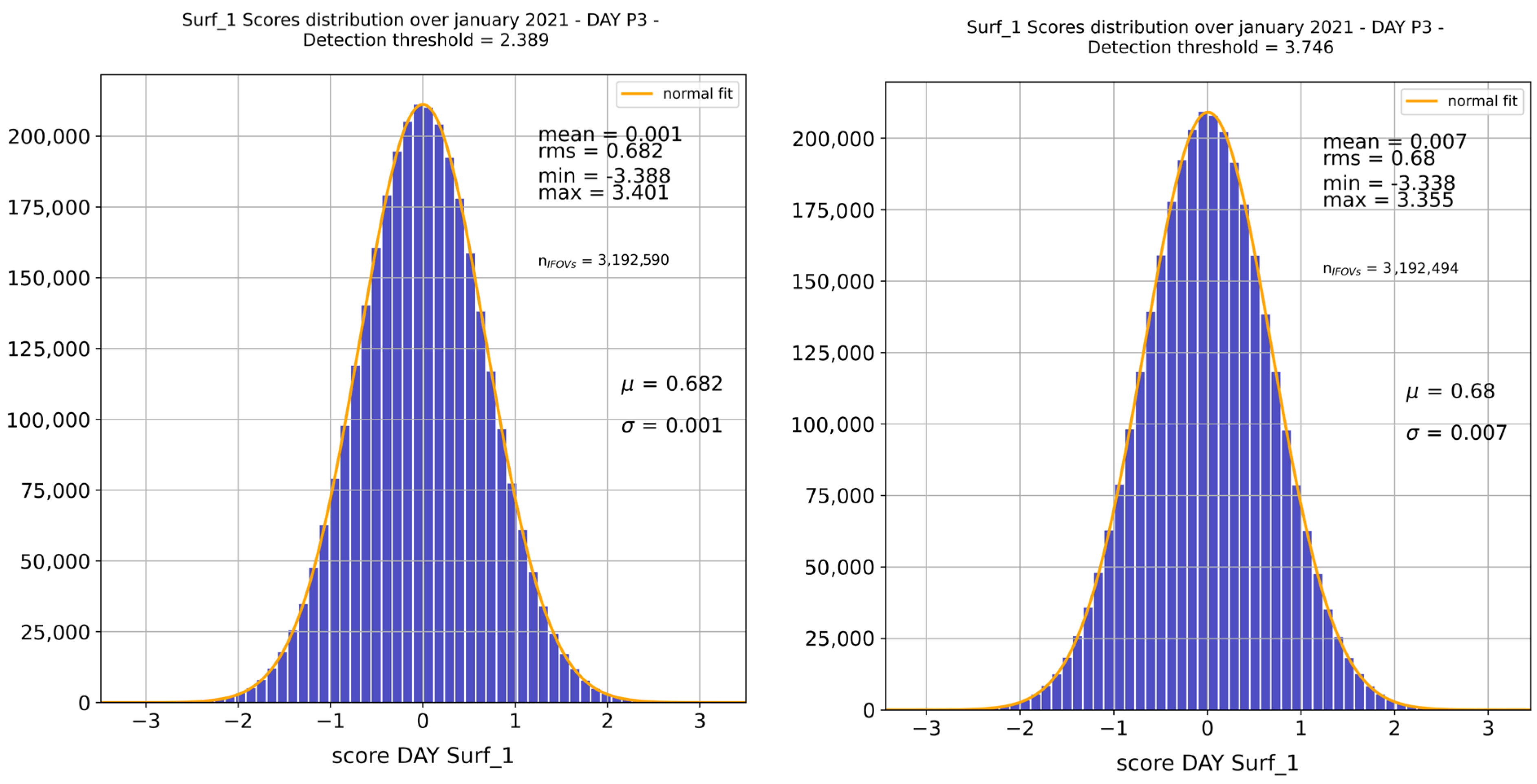
Figure A2.
Score distribution over January 2021 (IASI-C) before (left panel) and after (right panel) reference dataset cleaning for HCOOH_1 (IFOV P4, daytime, with a tolerance factor rising from to the retained . Sample size remains nearly unchanged after cleaning since this step affects only the reference basis and not the volume of analyzed data (January 2021).
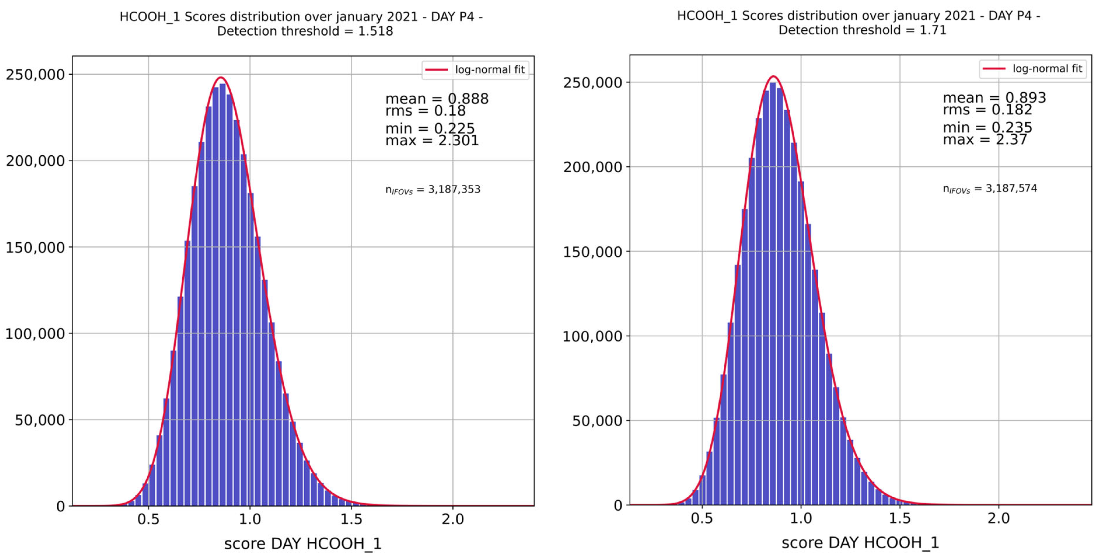
Appendix B. Methodological Choices
Appendix B.1. IASI Interbands
The two excluded interbands are defined by analyzing the first sub-diagonal of the correlation matrix noted and derived from the adjusted covariance matrix using Equation (A1) (where the index refers to the IASI spectral channels):
As shown in Figure A3, the correlation peaks observed at the interbands are excluded according to the following range, since they are associated with instrumental artifacts:
- B1/B2: [1149.75; 1224.75] cm−1;
- B2/B3: [1934.75; 2024.75] cm−1.
Figure A3.
First sub-diagonal of the correlation matrix calculated from the IASI-A noise covariance matrix (smoothed diagonals), for the 4 pixels. Vertical dashed lines show the chosen interband limits (B1/2 on the (left) and B2/B3 on the (right)).
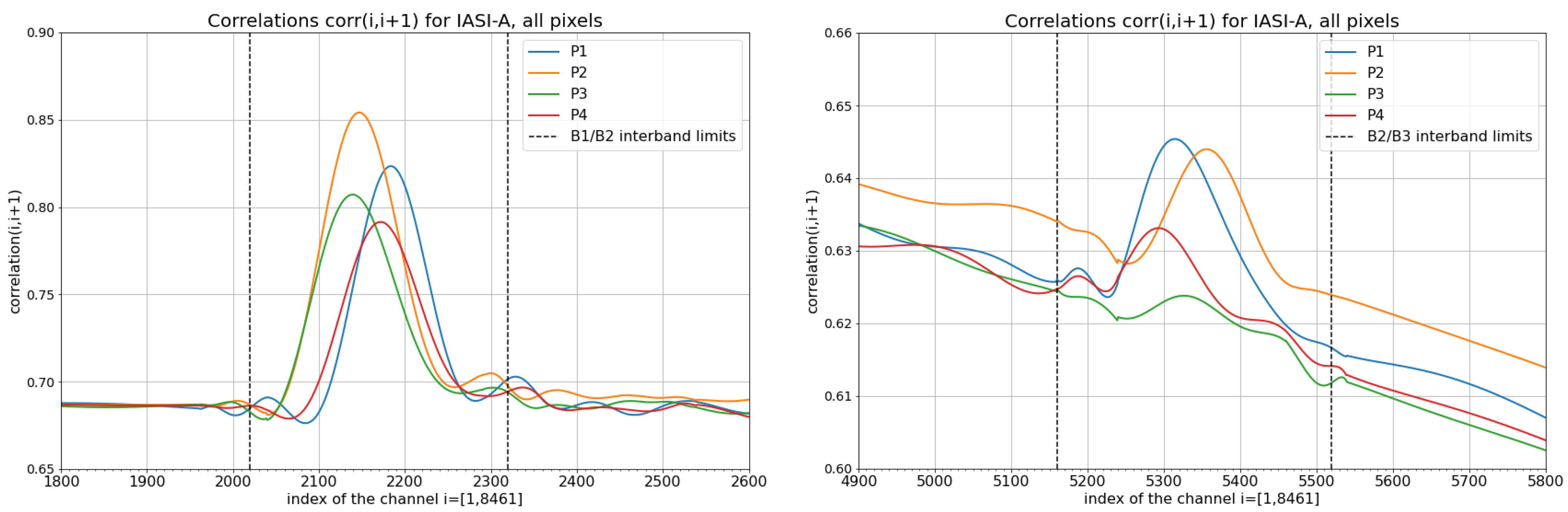
Appendix B.2. Adjustment of the Diagonal of the IASI Noise Covariance Matrix
Based on the original covariance matrix provided by CNES, the main diagonal of each IASI covariance matrix is smoothed and adjusted. This process removes the so-called “determination noise” induced by the calculation method of , which is empirically estimated from a limited number of on-board radiometric calibration blackbody views. Figure A4 shows an example of this adjustment for the case of IASI-A, pixel P1.
Figure A4.
Adjustment (red curve) of the IASI-A covariance matrix dated from November 2020 (black curve) for pixel P1, over different spectral intervals (expressed in channel numbers).
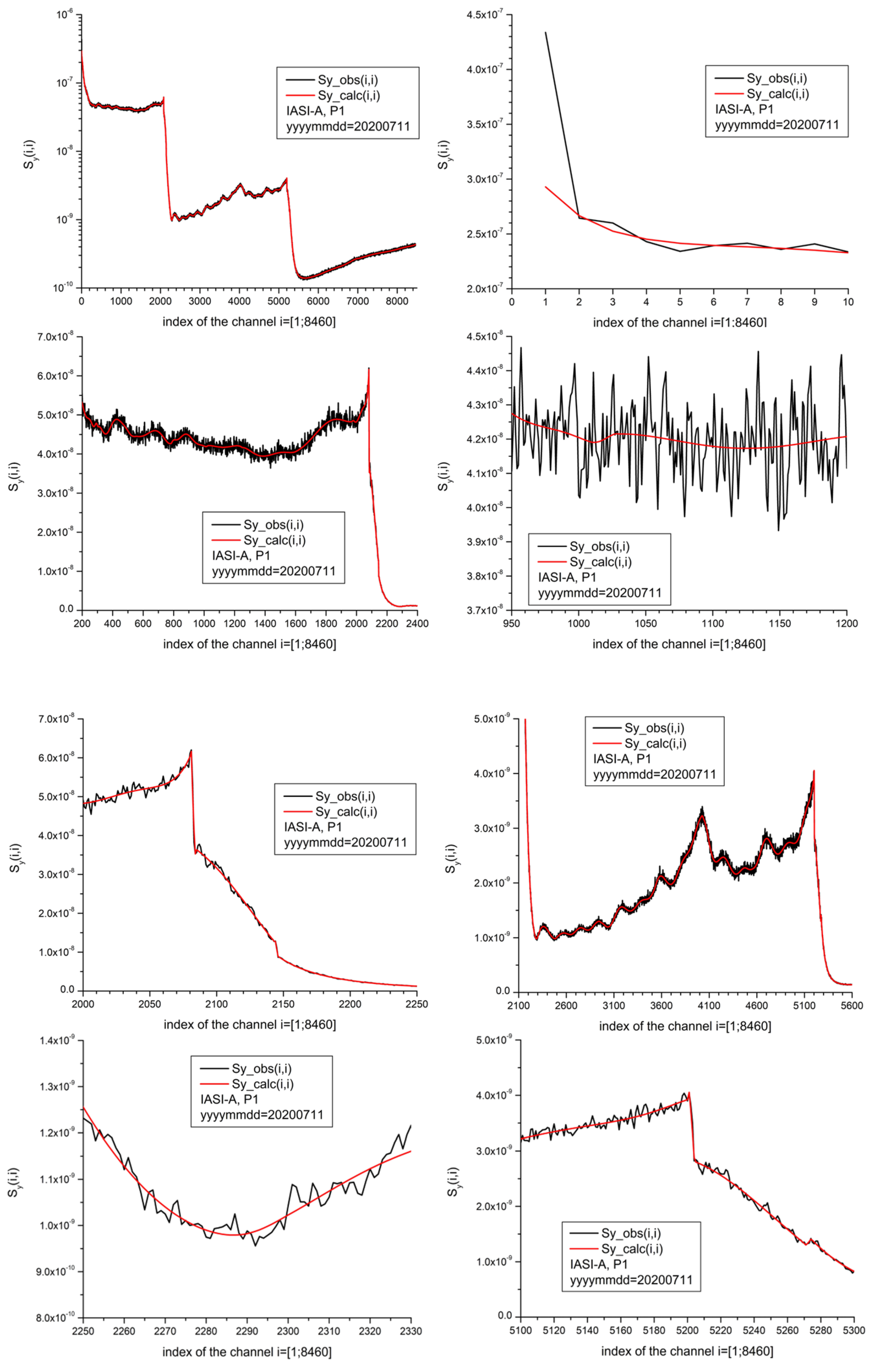
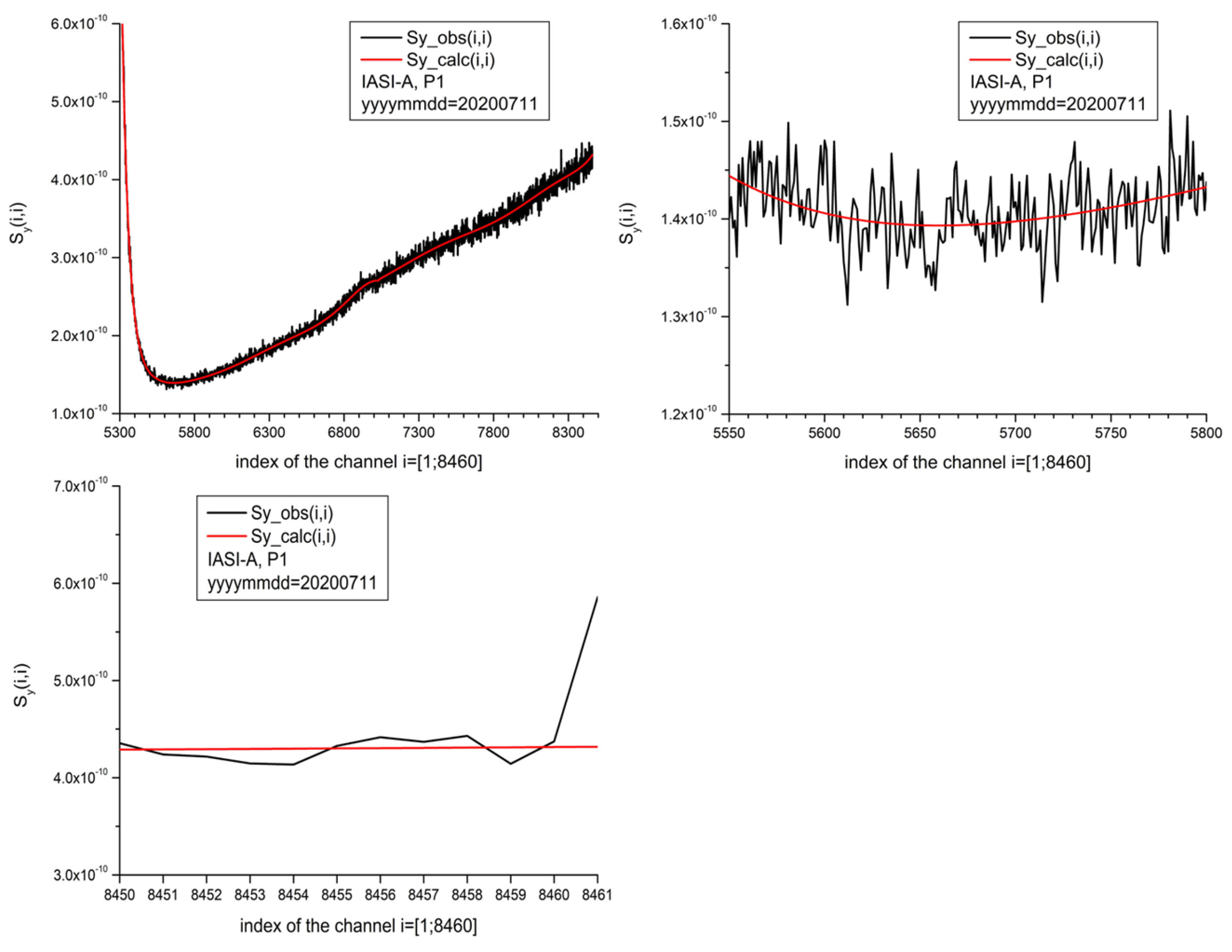
A piecewise polynomial fit is applied to the diagonal, providing a simplified, noise-free representation of the matrix, to a certain degree of inevitable approximation.
Appendix C. IASI-PCA Eigen-Structures
This appendix illustrates the fundamental roles of eigenvectors and eigenvalues within the IASI-PCA framework.
Appendix C.1. Eigenvalues and PCA Truncation
Figure A5 displays the eigenvalues obtained for each pixel of IASI-A, ordered from largest to smallest values. These curves are used to determine the truncation degree, that is, the number of principal components (PCs) retained for spectral projection and reconstruction.
Figure A5.
Scree plots obtained for pixel 1 of IASI-A—eigenvalues as a function of principal components for band B1 (blue curve), band B2 (orange curve) and band B3 (green curve). Truncation for each band is indicated by dashed vertical lines.
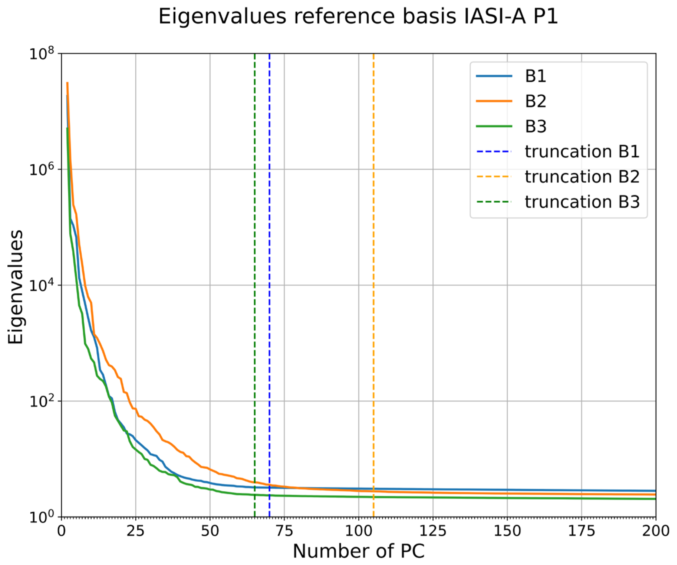
Given the large number of training sets considered here ( distinct datasets corresponding to the three IASI bands and four pixels), an automatic empirical method for determining the proper truncation was developed. The objective is to identify the “elbow” of the eigenvalues curve, i.e., the point from which the slope stabilizes and approaches zero. Figure A6 provides a concrete example of this method.
Figure A6.
Slope of the eigenvalues curve (blue curve) computed on the first 2000 principal components for IASI-A, pixel P1, band B1 (left panel) and zoom between the components 50 and 100 (right panel). The red curve is a moving average calculated on a window of 20 components. The horizontal gray lines show the chosen interval to determine the point from which the slope is considered sufficiently stable.
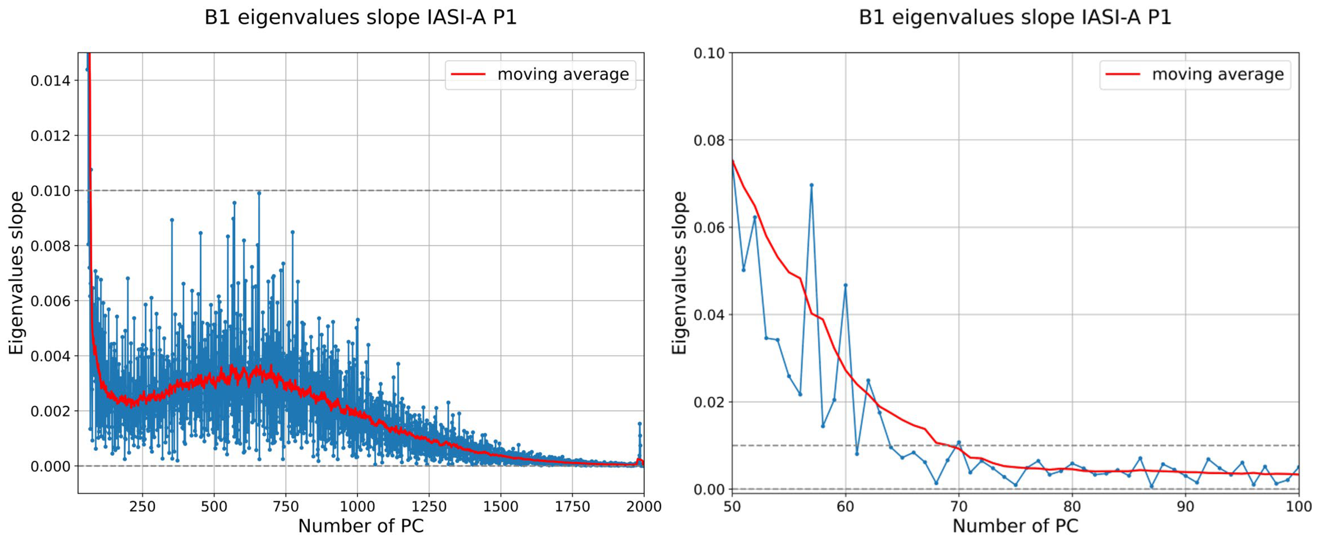
The truncation method follows four steps:
- Calculate the derivative of the eigenvalue curve for each band separately;
- Apply a moving average over a window of 20 principal components to smooth the noisy slope (cf. Figure A6, red curve);
- Define a stability interval given by [0, 0.01], where the slope is considered near zero (gray dotted line in Figure A6). The upper limit (0.01) was chosen empirically based on the inspection of the smoothed eigenvalue curves across all configurations;
- The truncation point is defined as the first principal component index for which the smoothed slope enters the interval [0, 0.01] and never exceeds 0.01 again for any subsequent component, over the full set of 8461 components computed. This criterion is applied independently to each IASI, band and IFOV configurations. The resulting truncation values range from 69 to 72 principal components for band B1, 103 to 114 for band B2, and 65 to 72 for band B3 (see Table A4). Given the limited dispersion observed across configurations within each band, a single representative truncation value per band, corresponding to the mean of the 12 configurations (rounded to the nearest multiple of 5), was chosen for operational simplicity in the processing, i.e., 70, 110 and 70 principal components, respectively, for bands B1, B2 and B3.
Table A4.
Number of principal components obtained for each configuration and retained values for the three IASI bands.
Appendix C.2. Eigenvectors
In the following, eigenvectors are sorted in order of decreasing eigenvalues. Figure A7 shows the first five eigenvectors derived from the IASI-A, pixel P1 training set, compared to eigenvectors 400–404.
Figure A7.
First five eigenvectors derived with the IASI-A, pixel P1 training set from 2020, sorted by decreasing eigenvalues (left panels), compared to the eigenvectors 400 to 404 (right panels).
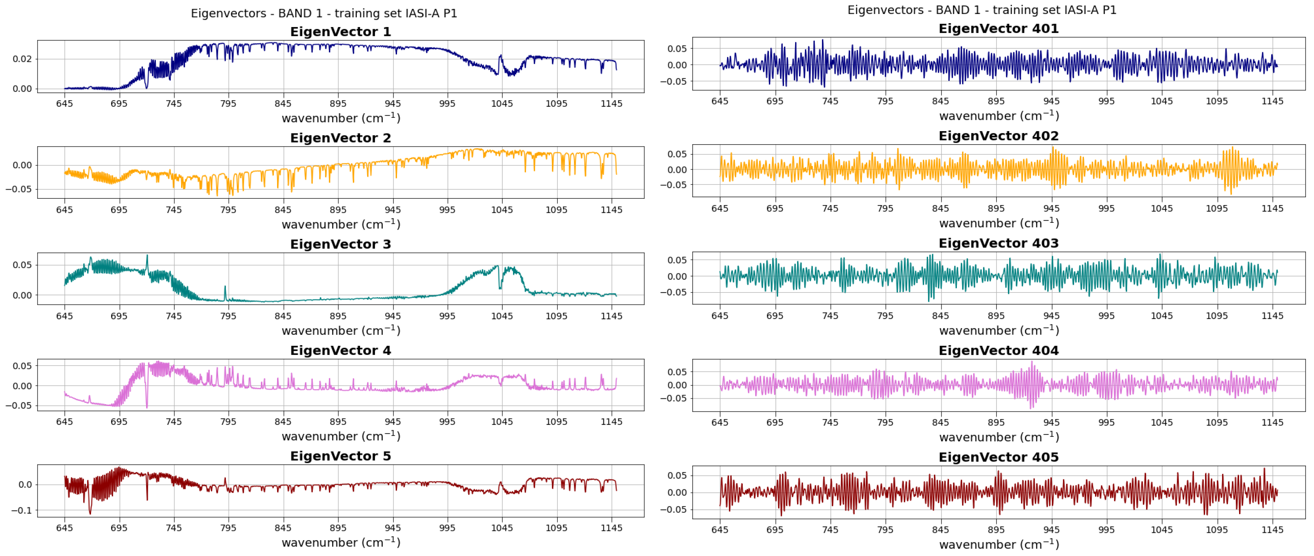
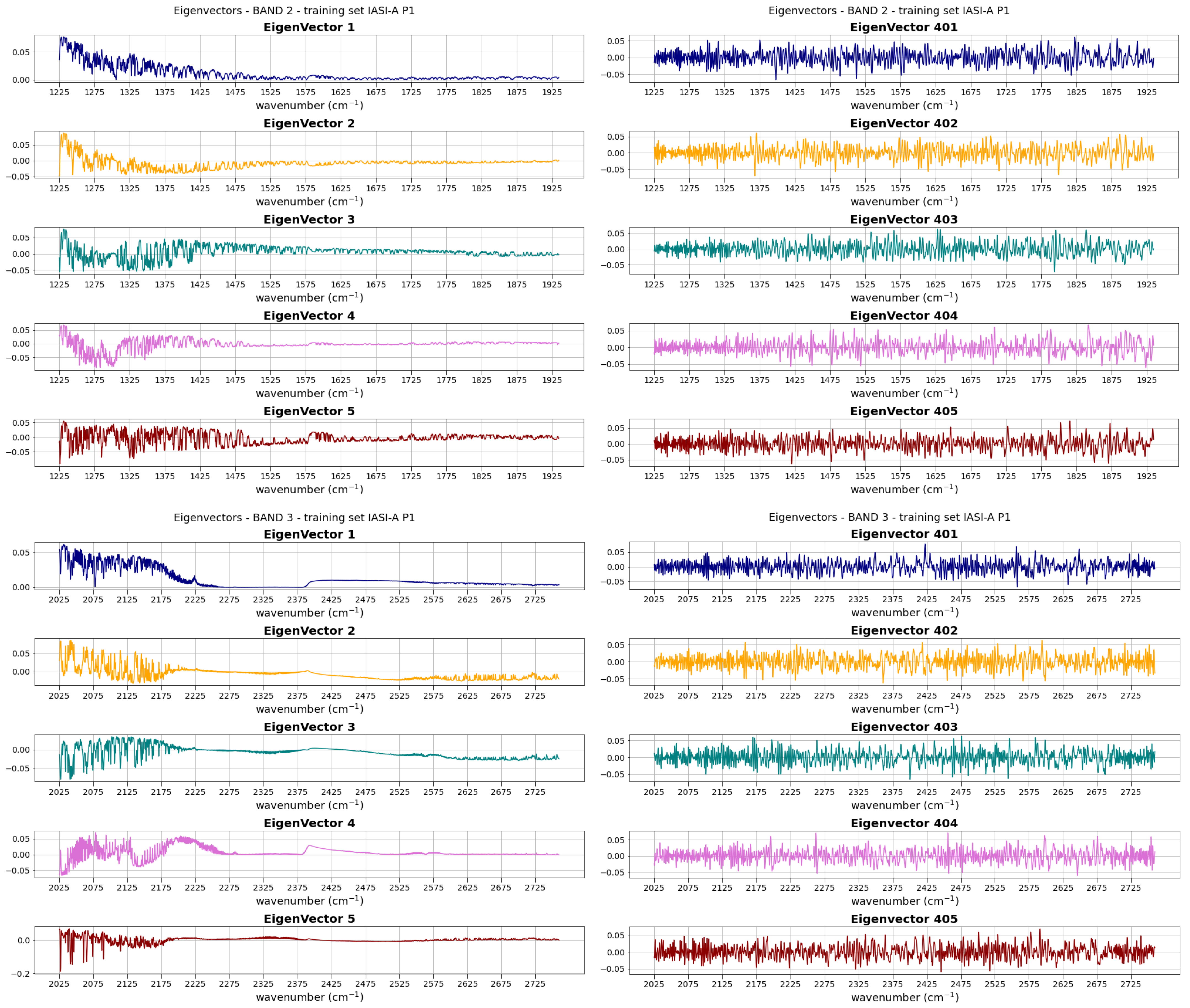
This demonstrates that signal and noise can be clearly separated, as mentioned before. In addition, it is interesting to note that the spectral signature of a given species is often spread across multiple eigenvectors rather than being concentrated in a single one.
References
- Intergovernmental Panel On Climate Change (IPCC). Climate Change 2021—The Physical Science Basis: Working Group I Contribution to the Sixth Assessment Report of the Intergovernmental Panel on Climate Change, 1st ed.; Cambridge University Press: Cambridge, UK, 2023. [Google Scholar]
- Abatzoglou, J.T.; Kolden, C.A.; Cullen, A.C.; Sadegh, M.; Williams, E.L.; Turco, M.; Jones, M.W. Climate Change Has Increased the Odds of Extreme Regional Forest Fire Years Globally. Nat. Commun. 2025, 16, 6390. [Google Scholar] [CrossRef] [Scilit] [PubMed]
- World Meteorological Organization (WMO). WMO Greenhouse Gas Bulletin: The State of Greenhouse Gases in the Atmosphere Using Global Observations up to December 2004; Bulletin No. 1; WMO: Geneva, Switzerland, 2006; pp. 1–4. [Google Scholar]
- Siméoni, D.; Singer, C.; Chalon, G. Infrared Atmospheric Sounding Interferometer. Acta Astronaut. 1997, 40, 113–118. [Google Scholar] [CrossRef] [Scilit]
- Huang, H.-L.; Antonelli, P. Application of Principal Component Analysis to High-Resolution Infrared Measurement Compression and Retrieval. J. Appl. Meteorol. Climatol. 2001, 40, 365–388. [Google Scholar] [CrossRef] [Scilit] [PubMed]
- Goldberg, M.D.; Zhou, L.; Wolf, W.; Barnet, C. Principal Component Analysis (PCA) of AIRS Data. In Proceedings of the ECMWF Workshop on Assimilation of High Spectral Resolution Sounders in NWP 2004, Reading, UK, 28 June–1 July 2004. [Google Scholar]
- EUMETSAT. IASI Level 1 PCC Product Generation Specification; EUMETSAT: Darmstadt, Germany, 2010. [Google Scholar]
- Collard, A.D.; McNally, A.P.; Hilton, F.I.; Healy, S.B.; Atkinson, N.C. The Use of Principal Component Analysis for the Assimilation of High-resolution Infrared Sounder Observations for Numerical Weather Prediction. Q. J. R. Meteorol. Soc. 2010, 136, 2038–2050. [Google Scholar] [CrossRef] [Scilit]
- Matricardi, M.; McNally, A.P. The Direct Assimilation of Principal Components of IASI Spectra in the ECMWF 4D-Var. Q. J. R. Meteorol. Soc. 2014, 140, 573–582. [Google Scholar] [CrossRef] [Scilit]
- Atkinson, N.C.; Hilton, F.I.; Illingworth, S.M.; Eyre, J.R.; Hultberg, T. Potential for the Use of Reconstructed IASI Radiances in the Detection of Atmospheric Trace Gases. Atmos. Meas. Tech. 2010, 3, 991–1003. [Google Scholar] [CrossRef] [Scilit]
- Clerbaux, C.; Boynard, A.; Clarisse, L.; George, M.; Hadji-Lazaro, J.; Herbin, H.; Hurtmans, D.; Pommier, M.; Razavi, A.; Turquety, S.; et al. Monitoring of Atmospheric Composition Using the Thermal Infrared IASI/MetOp Sounder. Atmos. Chem. Phys. 2009, 9, 6041–6054. [Google Scholar] [CrossRef] [Scilit]
- Turquety, S.; Hadji-Lazaro, J.; Clerbaux, C.; Hauglustaine, D.A.; Clough, S.A.; Cassé, V.; Schlüssel, P.; Mégie, G. Operational Trace Gas Retrieval Algorithm for the Infrared Atmospheric Sounding Interferometer. J. Geophys. Res. Atmos. 2004, 109, D21301. [Google Scholar] [CrossRef] [Scilit]
- George, M.; Clerbaux, C.; Hurtmans, D.; Turquety, S.; Coheur, P.-F.; Pommier, M.; Hadji-Lazaro, J.; Edwards, D.P.; Worden, H.; Luo, M.; et al. Carbon Monoxide Distributions from the IASI/METOP Mission: Evaluation with Other Space-Borne Remote Sensors. Atmos. Chem. Phys. 2009, 9, 8317–8330. [Google Scholar] [CrossRef] [Scilit]
- Clerbaux, C.; George, M.; Hadji-Lazaro, J.; Boynard, A.; Pommier, M.; Scannell, C.; Coheur, P.-F.; Hurtmans, D. Monitoring of Atmospheric Composition with the IASI/MetOP Sounder: Ozone and CO Distributions. In Proceedings of the 2009 EUMETSAT Meteorological Satellite Conference, Bath, UK, 21–25 September 2009. [Google Scholar]
- Crevoisier, C.; Chédin, A.; Matsueda, H.; Machida, T.; Armante, R.; Scott, N.A. First Year of Upper Tropospheric Integrated Content of CO2 from IASI Hyperspectral Infrared Observations. Atmos. Chem. Phys. 2009, 9, 4797–4810. [Google Scholar] [CrossRef] [Scilit]
- Coheur, P.-F.; Herbin, H.; Clerbaux, C.; Hurtmans, D.; Wespes, C.; Carleer, M.; Turquety, S.; Rinsland, C.P.; Remedios, J.; Hauglustaine, D.; et al. ACE-FTS Observation of a Young Biomass Burning Plume: First Reported Measurements of C2H4, C3H6O, H2CO and PAN by Infrared Occultation from Space. Atmos. Chem. Phys. 2007, 7, 5437–5446. [Google Scholar] [CrossRef] [Scilit]
- Pommier, M.; Clerbaux, C.; Coheur, P.-F.; Mahieu, E.; Müller, J.-F.; Paton-Walsh, C.; Stavrakou, T.; Vigouroux, C. HCOOH Distributions from IASI for 2008–2014: Comparison with Ground-Based FTIR Measurements and a Global Chemistry-Transport Model. Atmos. Chem. Phys. 2016, 16, 8963–8981. [Google Scholar] [CrossRef] [Scilit]
- Coheur, P.-F.; Clarisse, L.; Turquety, S.; Hurtmans, D.; Clerbaux, C. IASI Measurements of Reactive Trace Species in Biomass Burning Plumes. Atmos. Chem. Phys. 2009, 9, 5655–5667. [Google Scholar] [CrossRef] [Scilit]
- Xiao, Y.; Jacob, D.J.; Turquety, S. Atmospheric Acetylene and Its Relationship with CO as an Indicator of Air Mass Age. J. Geophys. Res. Atmos. 2007, 112, D12305. [Google Scholar] [CrossRef] [Scilit]
- Zhou, M.; Langerock, B.; Wang, P.; Vigouroux, C.; Ni, Q.; Hermans, C.; Dils, B.; Kumps, N.; Nan, W.; De Mazière, M. Understanding the Variations and Sources of CO, C2H2, C2H6, H2CO, and HCN Columns Based on 3 Years of New Ground-Based Fourier Transform Infrared Measurements at Xianghe, China. Atmos. Meas. Tech. 2023, 16, 273–293. [Google Scholar] [CrossRef] [Scilit]
- Duflot, V.; Hurtmans, D.; Clarisse, L.; R’honi, Y.; Vigouroux, C.; De Mazière, M.; Mahieu, E.; Servais, C.; Clerbaux, C.; Coheur, P.-F. Measurements of Hydrogen Cyanide (HCN) and Acetylene (C2H2) from the Infrared Atmospheric Sounding Interferometer (IASI). Atmos. Meas. Tech. 2013, 6, 917–925. [Google Scholar] [CrossRef] [Scilit]
- R’Honi, Y.; Clarisse, L.; Clerbaux, C.; Hurtmans, D.; Duflot, V.; Turquety, S.; Ngadi, Y.; Coheur, P.-F. Exceptional Emissions of NH3 and HCOOH in the 2010 Russian Wildfires. Atmos. Chem. Phys. 2013, 13, 4171–4181. [Google Scholar] [CrossRef] [Scilit]
- Franco, B.; Clarisse, L.; Stavrakou, T.; Müller, J.-F.; Van Damme, M.; Whitburn, S.; Hadji-Lazaro, J.; Hurtmans, D.; Taraborrelli, D.; Clerbaux, C.; et al. A General Framework for Global Retrievals of Trace Gases From IASI: Application to Methanol, Formic Acid, and PAN. J. Geophys. Res. Atmos. 2018, 123, 13,963–13,984. [Google Scholar] [CrossRef] [Scilit]
- Van Damme, M.; Clarisse, L.; Whitburn, S.; Hadji-Lazaro, J.; Hurtmans, D.; Clerbaux, C.; Coheur, P.-F. Industrial and Agricultural Ammonia Point Sources Exposed. Nature 2018, 564, 99–103. [Google Scholar] [CrossRef] [Scilit] [PubMed]
- Whitburn, S.; Van Damme, M.; Clarisse, L.; Turquety, S.; Clerbaux, C.; Coheur, P.-F. Doubling of Annual Ammonia Emissions from the Peat Fires in Indonesia during the 2015 El Niño. Geophys. Res. Lett. 2016, 43, 11,007–11,014. [Google Scholar] [CrossRef] [Scilit]
- Clarisse, L.; Franco, B.; Van Damme, M.; Di Gioacchino, T.; Hadji-Lazaro, J.; Whitburn, S.; Noppen, L.; Hurtmans, D.; Clerbaux, C.; Coheur, P. The IASI NH3 Version 4 Product: Averaging Kernels and Improved Consistency. Atmos. Meas. Tech. 2023, 16, 5009–5028. [Google Scholar] [CrossRef] [Scilit]
- Clarisse, L.; Coheur, P.F.; Prata, A.J.; Hurtmans, D.; Razavi, A.; Phulpin, T.; Hadji-Lazaro, J.; Clerbaux, C. Tracking and Quantifying Volcanic SO2 with IASI, the September 2007 Eruption at Jebel at Tair. Atmos. Chem. Phys. 2008, 8, 7723–7734. [Google Scholar] [CrossRef] [Scilit]
- Clarisse, L.; Franco, B.; Fabris, L.; Theys, N.; Hadji-Lazaro, J.; Hurtmans, D.; Clerbaux, C.; Coheur, P. An 18-Year Record of Atmospheric Sulphur Dioxide (SO2) Derived from IASI Measurements. Earth Syst. Sci. Data Discuss. 2026. in review. [Google Scholar] [CrossRef] [Scilit]
- Kok, J.F.; Storelvmo, T.; Karydis, V.A.; Adebiyi, A.A.; Mahowald, N.M.; Evan, A.T.; He, C.; Leung, D.M. Mineral Dust Aerosol Impacts on Global Climate and Climate Change. Nat. Rev. Earth Environ. 2023, 4, 71–86. [Google Scholar] [CrossRef] [Scilit]
- Loskot, J.; Jezbera, D.; Nalezinková, M.; Šmejkalová, A.H.; Fernandes, D.; Komárek, J. Impact of Saharan Dust on Particulate Matter Characteristics in an Urban and a Natural Locality in Central Europe. Sci. Rep. 2024, 14, 32002. [Google Scholar] [CrossRef] [Scilit] [PubMed]
- Vu Van, A.; Boynard, A.; Prunet, P.; Jolivet, D.; Lezeaux, O.; Henry, P.; Camy-Peyret, C.; Clarisse, L.; Franco, B.; Coheur, P.-F.; et al. Near-Real-Time Detection of Unexpected Atmospheric Events Using Principal Component Analysis on the Infrared Atmospheric Sounding Interferometer (IASI) Radiances. Atmos. Meas. Tech. 2023, 16, 2107–2127. [Google Scholar] [CrossRef] [Scilit]
- Gordon, I.; Rothman, L.; Hargreaves, R.; Gomez, F.; Bertin, T.; Hill, C.; Kochanov, R.; Tan, Y.; Wcisło, P.; Makhnev, V.; et al. The HITRAN2024 Molecular Spectroscopic Database. J. Quant. Spectrosc. Radiat. Transf. 2026, 353, 109807. [Google Scholar] [CrossRef] [Scilit]
- Delahaye, T.; Armante, R.; Scott, N.A.; Jacquinet-Husson, N.; Chédin, A.; Crépeau, L.; Crevoisier, C.; Douet, V.; Perrin, A.; Barbe, A.; et al. The 2020 Edition of the GEISA Spectroscopic Database. J. Mol. Spectrosc. 2021, 380, 111510. [Google Scholar] [CrossRef] [Scilit]
- EUMETSAT. Product User Guide—IASI PCS Release 1; EUMETSAT: Darmstadt, Germany, 2024; Available online: https://user.eumetsat.int/s3/eup-strapi-media/Product_User_Guide_IASI_PCS_release_1_382d1df483.pdf (accessed on 26 July 2026).
- EUMETSAT. IASI Level-1 Product Guide; EUMETSAT: Darmstadt, Germany, 2019; Available online: https://user.eumetsat.int/s3/eup-strapi-media/pdf_iasi_pg_487c765315.pdf (accessed on 26 July 2026).
- Antonelli, P.; Revercomb, H.E.; Sromovsky, L.A.; Smith, W.L.; Knuteson, R.O.; Tobin, D.C.; Garcia, R.K.; Howell, H.B.; Huang, H.-L.; Best, F.A. A Principal Component Noise Filter for High Spectral Resolution Infrared Measurements. J. Geophys. Res. Atmos. 2004, 109, D23102. [Google Scholar] [CrossRef] [Scilit]
- Hultberg, T. IASI Principal Component Compression (IASI PCC) FAQ 2009. Available online: https://www.google.com/url?sa=t&source=web&rct=j&opi=89978449&url=https://user.eumetsat.int/s3/eup-strapi-media/pdf_ipcc_faq_680c5f230c.pdf&ved=2ahUKEwjb4uLbl_eVAxUcfKQEHdkUPRkQFnoECBgQAQ&usg=AOvVaw1Cy95SffUJqvCuKon2CQox (accessed on 26 July 2026).
- EUMETSAT. IASI Level 1 Product Format Specification; EUMETSAT: Darmstadt, Germany, 2011. [Google Scholar]
- Dowlatshah, M.; Ghassemian, H.; Imani, M. Spatial-spectral morphological feature extraction for hyperspectral images classification. Int. Arch. Photogramm. Remote Sens. Spat. Inf. Sci. 2019, XLII-4-W18, 315–320. [Google Scholar] [CrossRef] [Scilit]
- Rishikeshan, C.A.; Ramesh, H. An Automated Mathematical Morphology Driven Algorithm for Water Body Extraction from Remotely Sensed Images. ISPRS J. Photogramm. Remote Sens. 2018, 146, 11–21. [Google Scholar] [CrossRef] [Scilit]
- European Commission, Joint Research Centre. Fire in Var, France (2021-08-17). 2026. Available online: http://data.europa.eu/89h/492f5467-b604-49c8-8695-f0b219880eaf (accessed on 26 July 2026).
- Walker, J.C.; Dudhia, A.; Carboni, E. An Effective Method for the Detection of Trace Species Demonstrated Using the MetOp Infrared Atmospheric Sounding Interferometer. Atmos. Meas. Tech. 2011, 4, 1567–1580. [Google Scholar] [CrossRef] [Scilit]
- Clarisse, L.; Coheur, P.-F.; Prata, F.; Hadji-Lazaro, J.; Hurtmans, D.; Clerbaux, C. A Unified Approach to Infrared Aerosol Remote Sensing and Type Specification. Atmos. Chem. Phys. 2013, 13, 2195–2221. [Google Scholar] [CrossRef] [Scilit]
- Müller, C.M.; Pejcic, B.; Esteban, L.; Piane, C.D.; Raven, M.; Mizaikoff, B. Infrared Attenuated Total Reflectance Spectroscopy: An Innovative Strategy for Analyzing Mineral Components in Energy Relevant Systems. Sci. Rep. 2014, 4, 6764. [Google Scholar] [CrossRef] [Scilit] [PubMed]
- Francis, D.; Chaboureau, J.-P.; Nelli, N.; Cuesta, J.; Alshamsi, N.; Temimi, M.; Pauluis, O.; Xue, L. Summertime Dust Storms over the Arabian Peninsula and Impacts on Radiation, Circulation, Cloud Development and Rain. Atmos. Res. 2021, 250, 105364. [Google Scholar] [CrossRef] [Scilit]
- Kaufman, Y.J.; Tanré, D.; Remer, L.A.; Vermote, E.F.; Chu, A.; Holben, B.N. Operational Remote Sensing of Tropospheric Aerosol over Land from EOS Moderate Resolution Imaging Spectroradiometer. J. Geophys. Res. Atmos. 1997, 102, 17051–17067. [Google Scholar] [CrossRef] [Scilit]
- Aminou, D.M.A. MSG’s SEVIRI Instrument; ESTEC: Noordwijk, The Netherlands, 2002. [Google Scholar]
- Capelle, V.; Chédin, A.; Siméon, M.; Tsamalis, C.; Pierangelo, C.; Pondrom, M.; Crevoisier, C.; Crepeau, L.; Scott, N.A. Evaluation of IASI-Derived Dust Aerosol Characteristics over the Tropical Belt. Atmos. Chem. Phys. 2014, 14, 9343–9362. [Google Scholar] [CrossRef] [Scilit]
- Capelle, V.; Chédin, A.; Pondrom, M.; Crevoisier, C.; Armante, R.; Crepeau, L.; Scott, N.A. Infrared Dust Aerosol Optical Depth Retrieved Daily from IASI and Comparison with AERONET over the Period 2007–2016. Remote Sens. Environ. 2018, 206, 15–32. [Google Scholar] [CrossRef] [Scilit]
- Hultberg, T. Hybrid Principal Component (PC) Compression, International TOVS Working Group. Available online: https://www.google.com/url?sa=t&source=web&rct=j&opi=89978449&url=https://itwg.ssec.wisc.edu/wordpress/wp-content/uploads/2023/05/poster.6p.06.Hultberg-Tim-Hultberg_itsc24.pdf&ved=2ahUKEwiOjpmclPeVAxXJVqQEHYeeGoEQFnoECBkQAQ&usg=AOvVaw0B5ea6ZnwwFHQEkSdK4HJs (accessed on 26 July 2026).
- Abd El-Rahman Hegab, M.; Abou El Magd, I.; Hamed Abd El Wahid, K. Revealing Potential Mineralization Zones Utilizing Landsat-9, ASTER and Airborne Radiometric Data at Elkharaza-Dara Area, North Eastern Desert, Egypt. Egypt. J. Remote Sens. Space Sci. 2024, 27, 716–733. [Google Scholar] [CrossRef] [Scilit]
- Masek, J.G.; Wulder, M.A.; Markham, B.; McCorkel, J.; Crawford, C.J.; Storey, J.; Jenstrom, D.T. Landsat 9: Empowering Open Science and Applications through Continuity. Remote Sens. Environ. 2020, 248, 111968. [Google Scholar] [CrossRef] [Scilit]
- Yamaguchi, Y.; Kahle, A.B.; Tsu, H.; Kawakami, T.; Pniel, M. Overview of Advanced Spaceborne Thermal Emission and Reflection Radiometer (ASTER). IEEE Trans. Geosci. Remote Sens. 1998, 36, 1062–1071. [Google Scholar] [CrossRef] [Scilit]
- Powers, R.W.; Ramirez, L.F.; Redmond, C.D.; Elberg, E.L., Jr. Geology of the Arabian Peninsula, Sedimentary Geology of Saudi Arabia; U.S. Geological Survey Professional Paper 560-D; United States Government Printing Office: Washington, DC, USA, 1966. [Google Scholar]
- Alalam, P.; Deschutter, L.; Al Choueiry, A.; Petitprez, D.; Herbin, H. Aerosol Mineralogical Study Using Laboratory and IASI Measurements: Application to East Asian Deserts. Remote Sens. 2022, 14, 3422. [Google Scholar] [CrossRef] [Scilit]
- Clarisse, L.; Clerbaux, C.; Dentener, F.; Hurtmans, D.; Coheur, P.-F. Global Ammonia Distribution Derived from Infrared Satellite Observations. Nat. Geosci. 2009, 2, 479–483. [Google Scholar] [CrossRef] [Scilit]
- Sheng, M.; Zhou, R.; Hua, J.; Han, S.; Zhang, L.; Wang, W.; Dang, R.; Cao, H.; Chen, Z.; Gu, Y.; et al. Geostationary Observations of Atmospheric Ammonia over East Asia: Spatio-Temporal Variations Revealed by Three Years of FY-4B/GIIRS Measurements. Atmos. Chem. Phys. 2026, 26, 7803–7826. [Google Scholar] [CrossRef] [Scilit]
- Shephard, M.W.; Cady-Pereira, K.E. Cross-Track Infrared Sounder (CrIS) Satellite Observations of Tropospheric Ammonia. Atmos. Meas. Tech. 2015, 8, 1323–1336. [Google Scholar] [CrossRef] [Scilit]
- Safieddine, S.; Parracho, A.C.; George, M.; Aires, F.; Pellet, V.; Clarisse, L.; Whitburn, S.; Lezeaux, O.; Thépaut, J.-N.; Hersbach, H.; et al. Artificial Neural Networks to Retrieve Land and Sea Skin Temperature from IASI. Remote Sens. 2020, 12, 2777. [Google Scholar] [CrossRef] [Scilit]
- Bouillon, M.; Safieddine, S.; Whitburn, S.; Clarisse, L.; Aires, F.; Pellet, V.; Lezeaux, O.; Scott, N.A.; Doutriaux-Boucher, M.; Clerbaux, C. Time Evolution of Temperature Profiles Retrieved from 13 Years of Infrared Atmospheric Sounding Interferometer (IASI) Data Using an Artificial Neural Network. Atmos. Meas. Tech. 2022, 15, 1779–1793. [Google Scholar] [CrossRef] [Scilit]
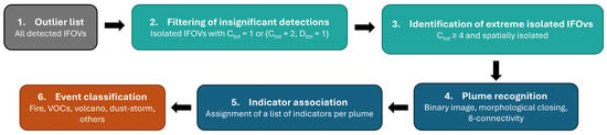
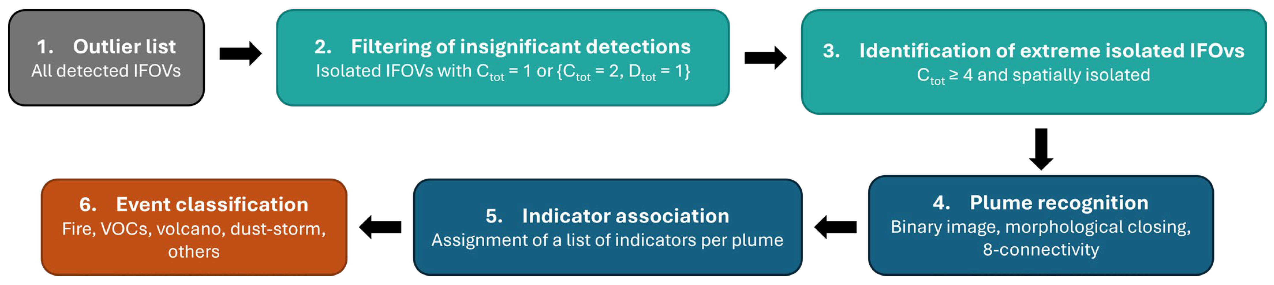
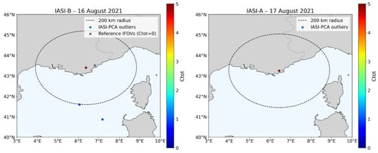
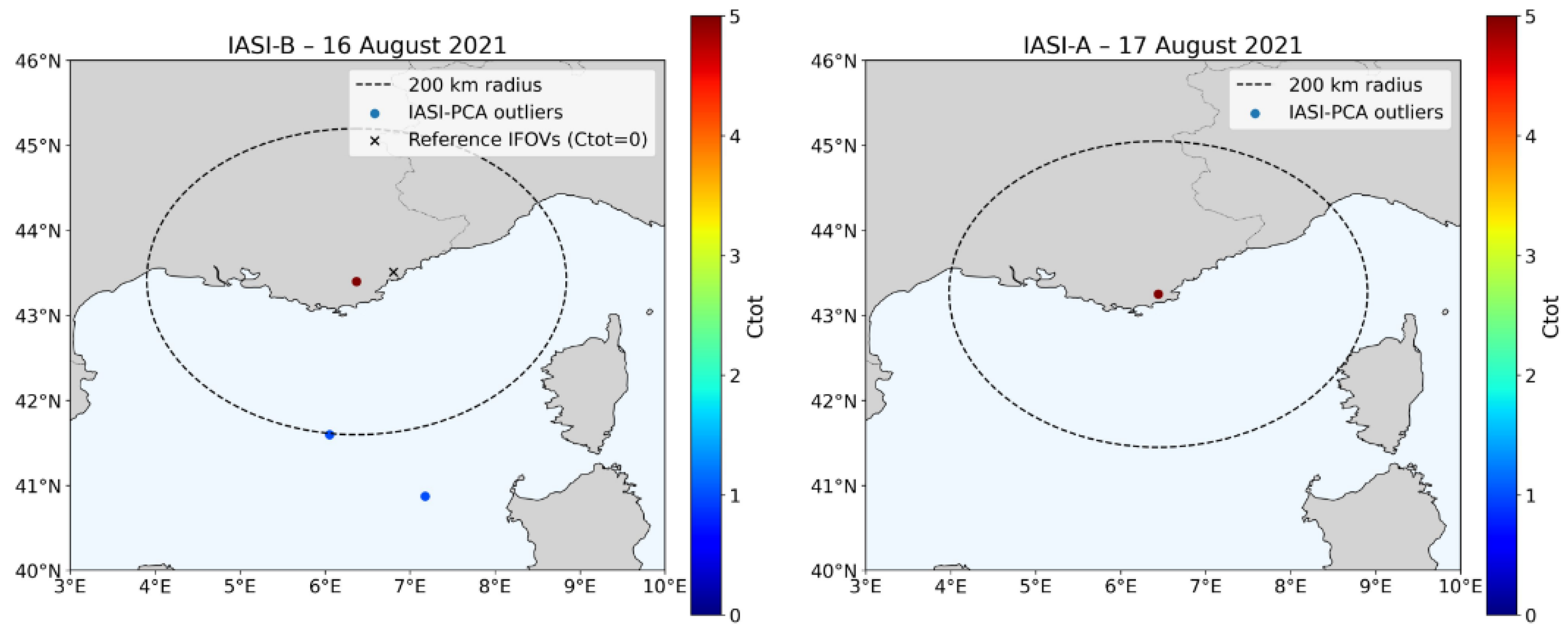
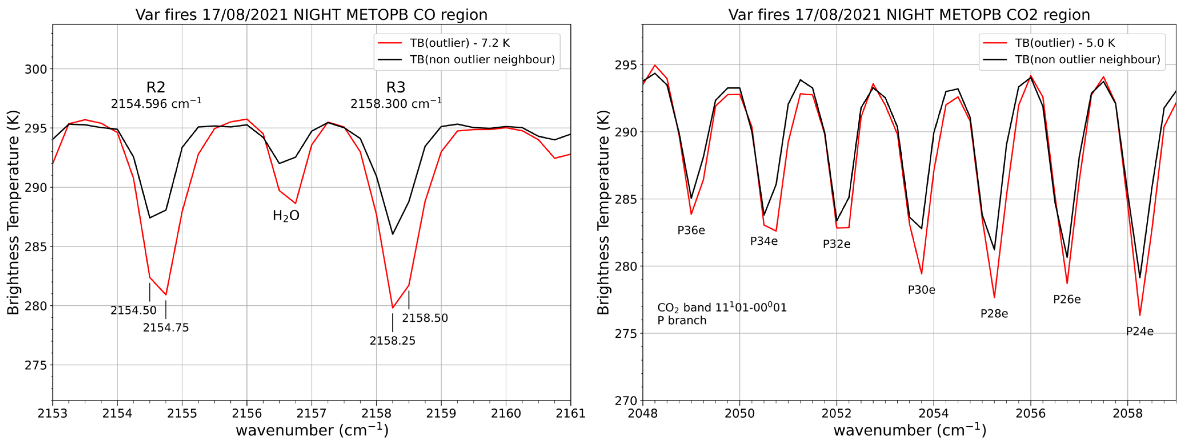
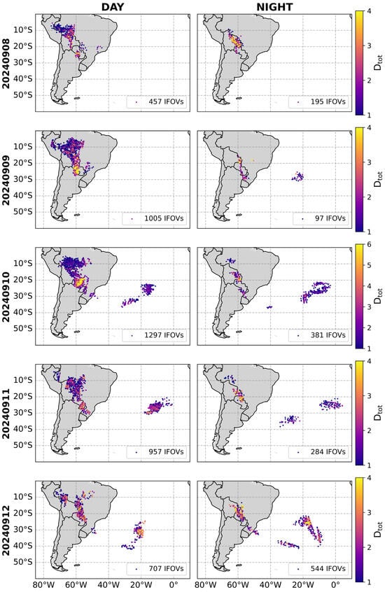
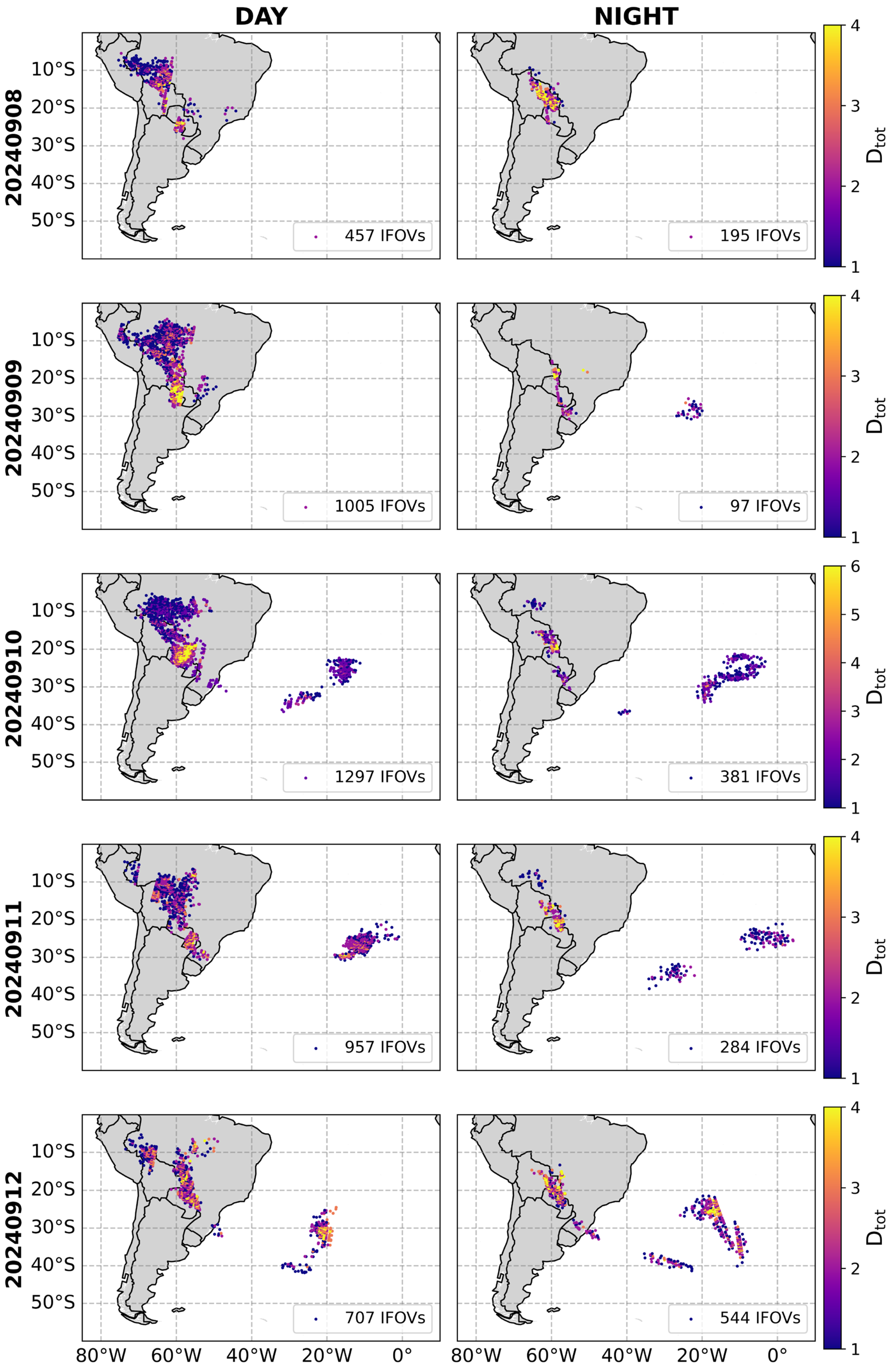
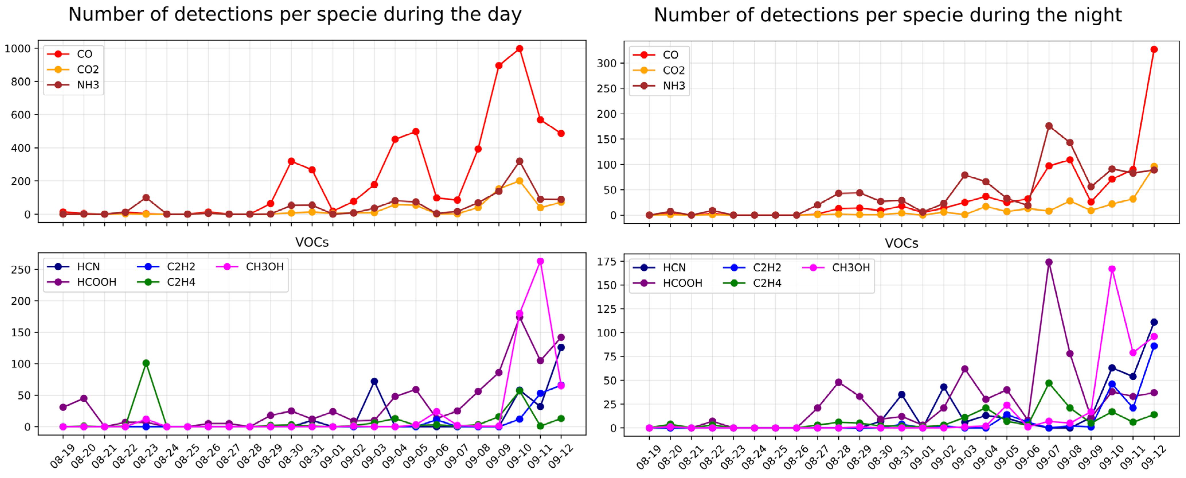
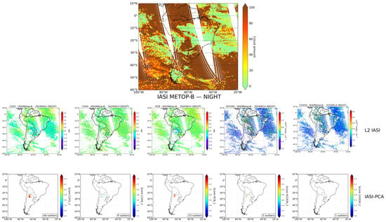
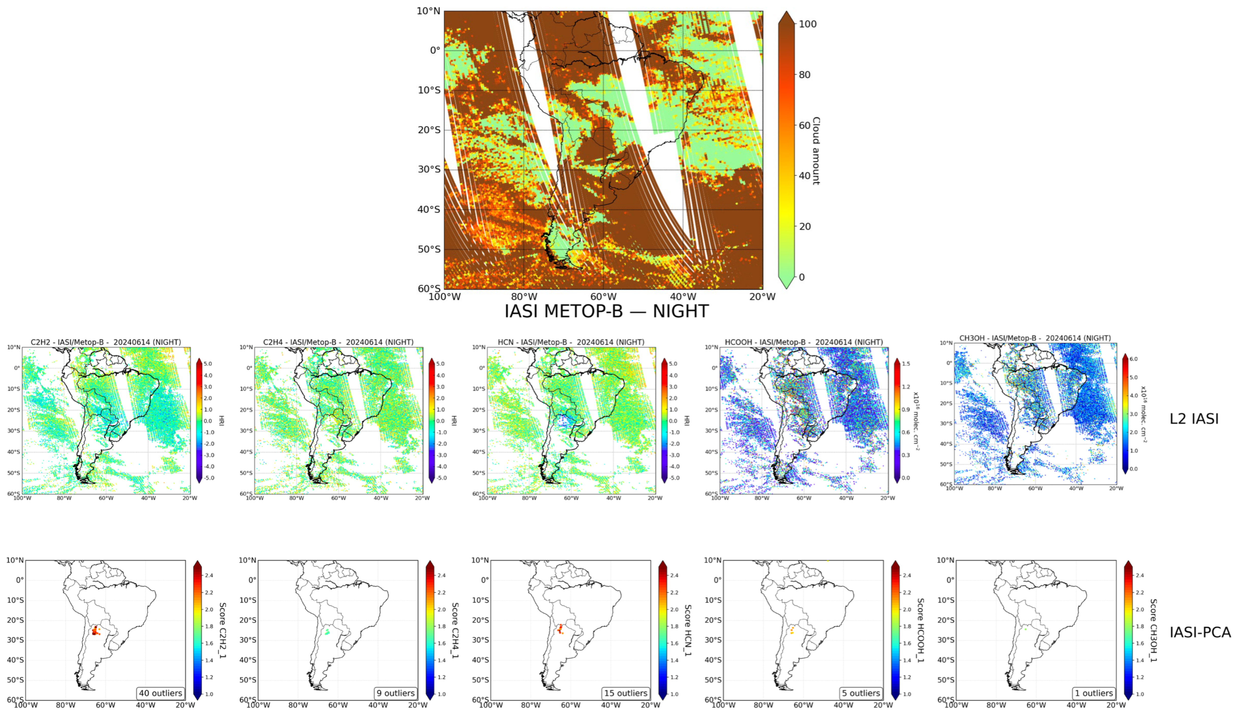
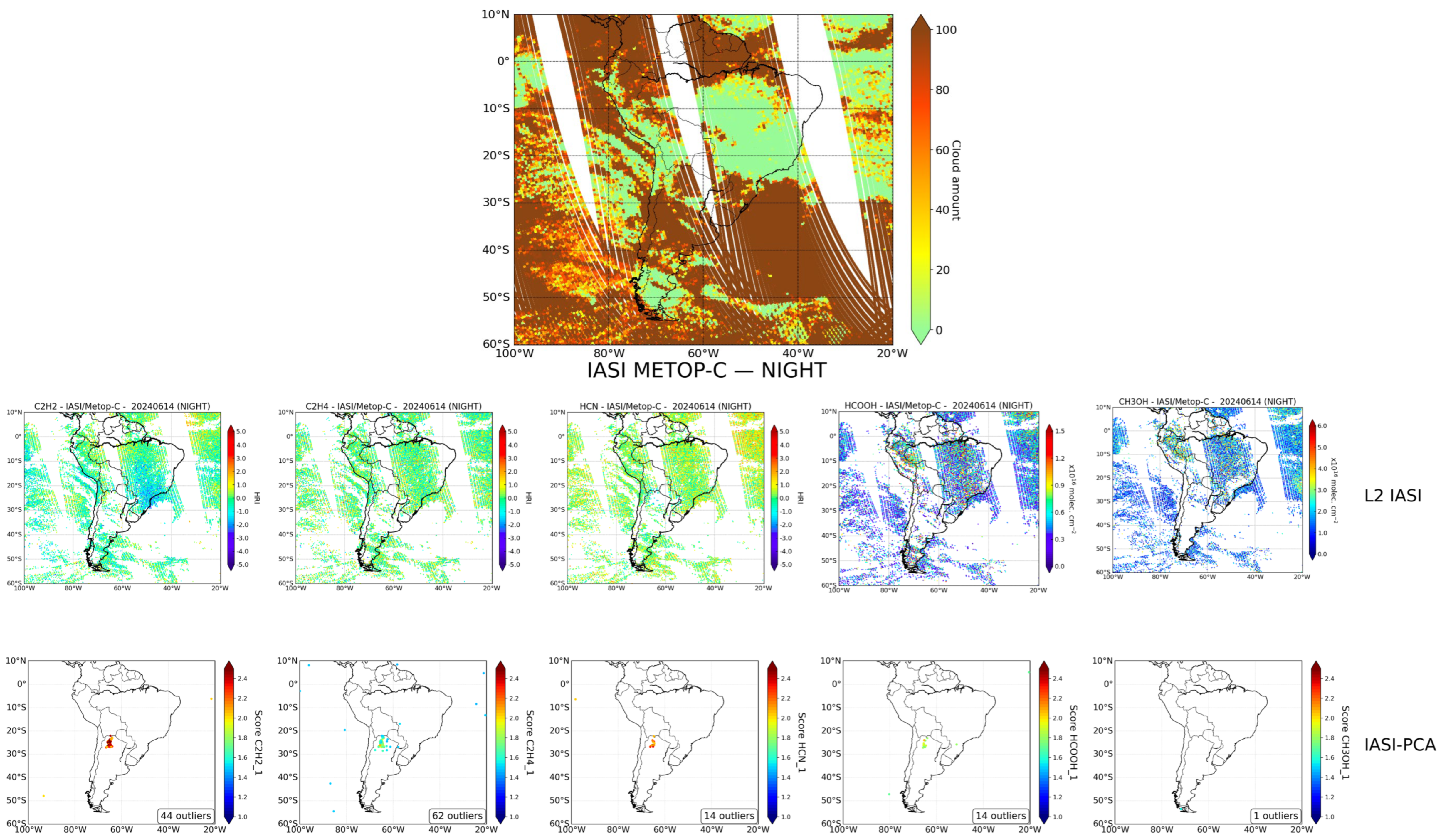
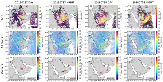
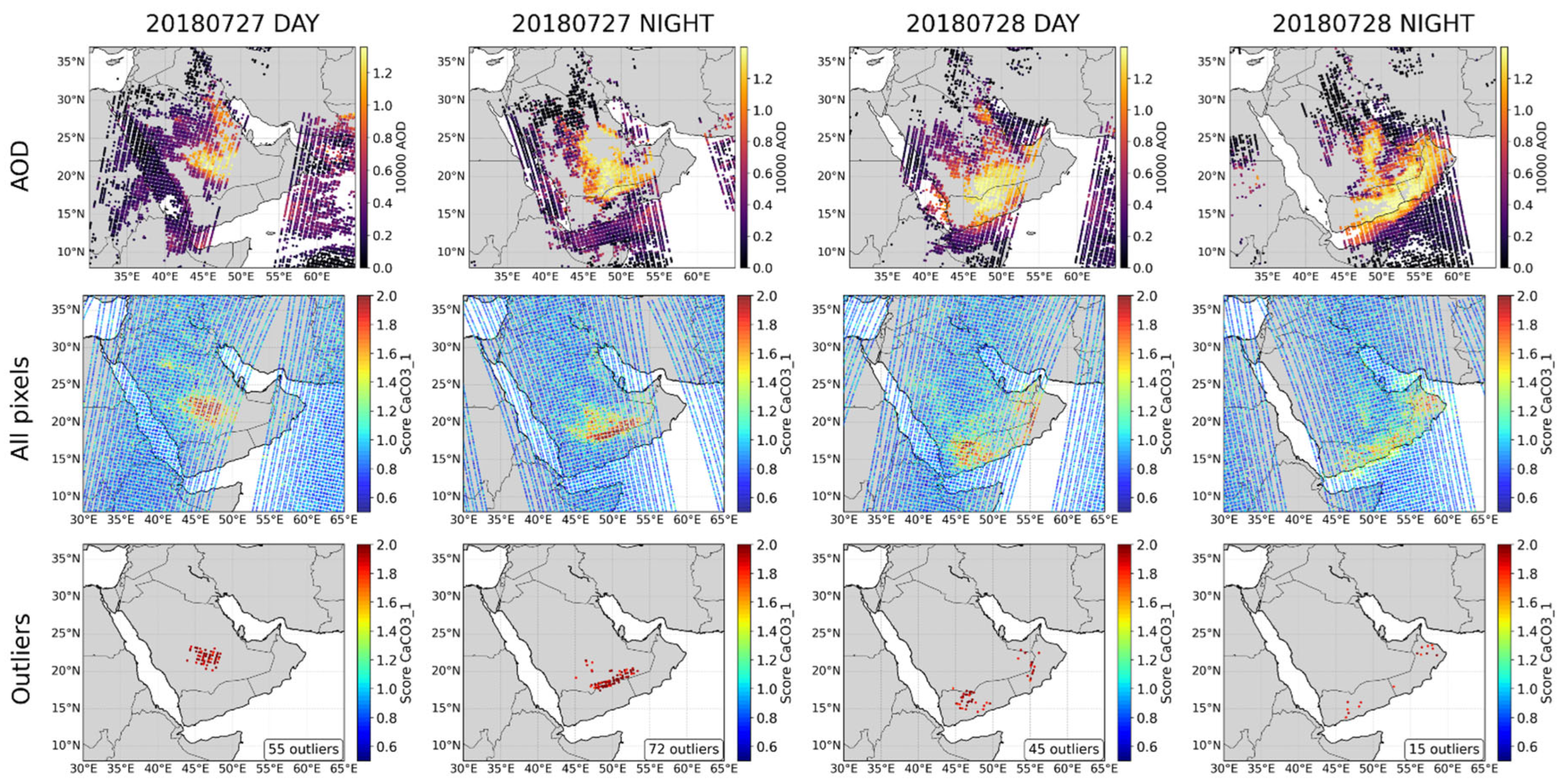
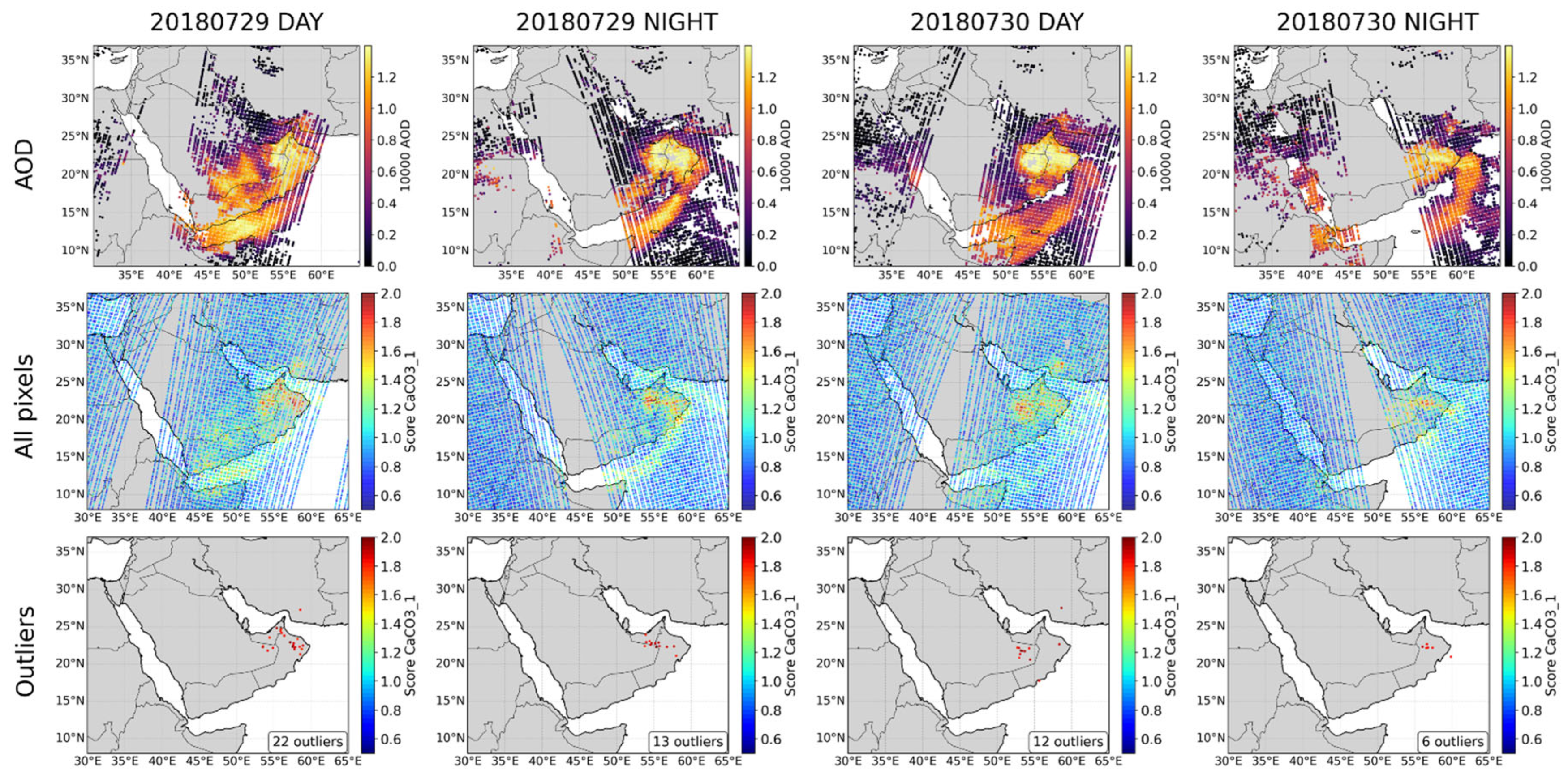
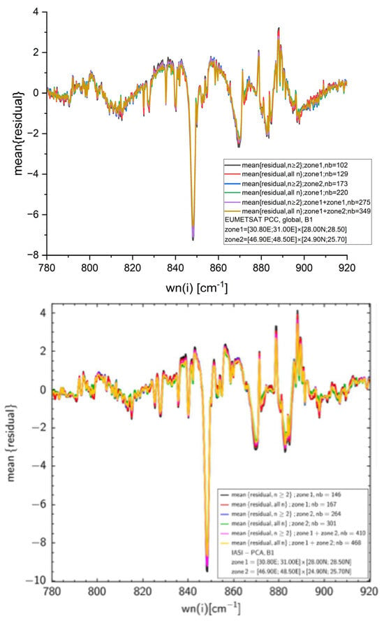
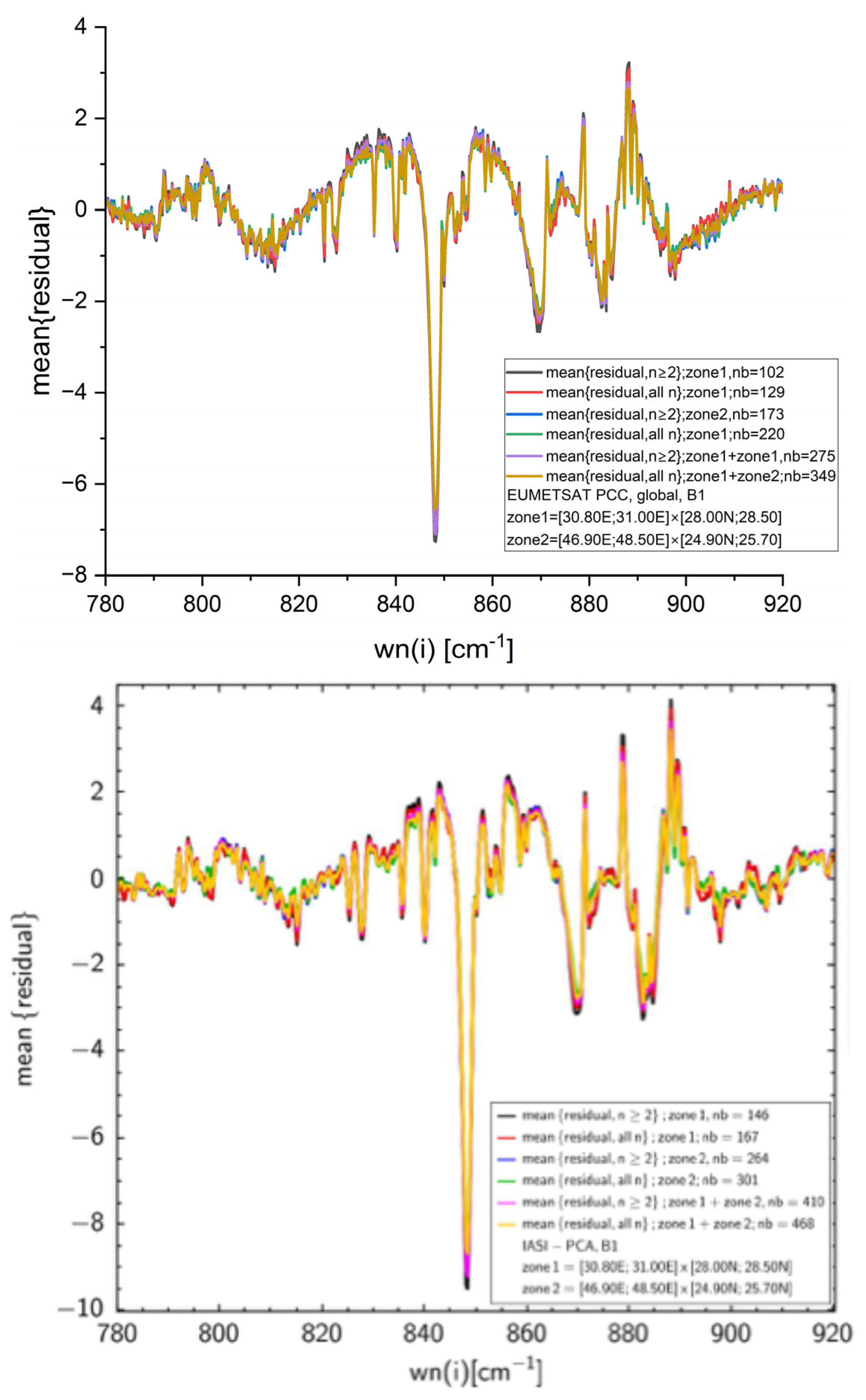
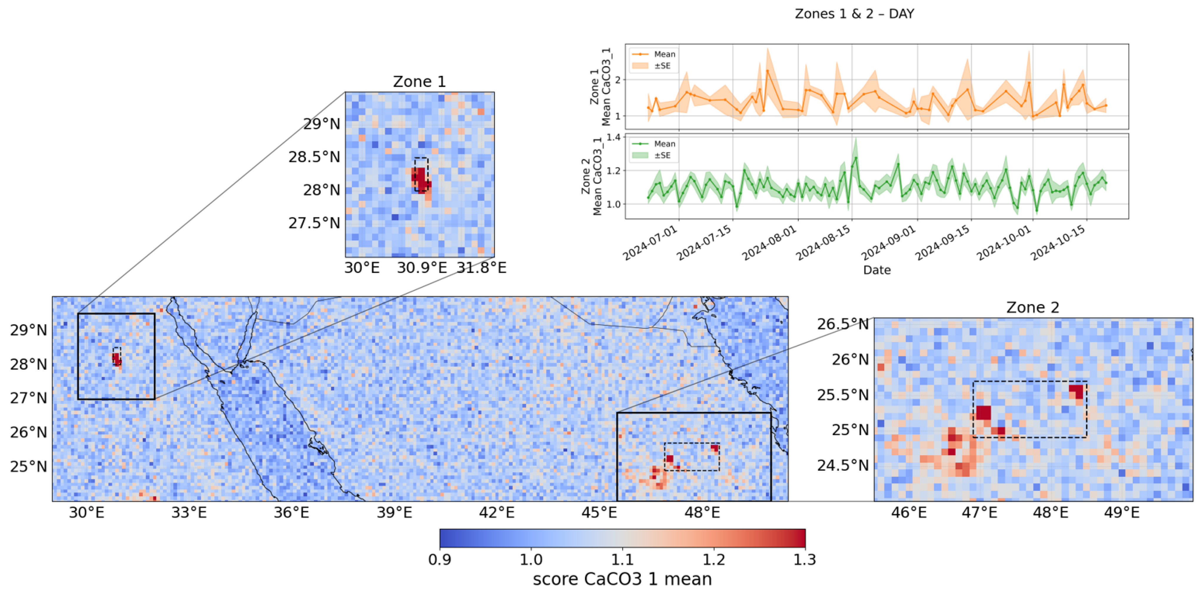
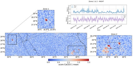
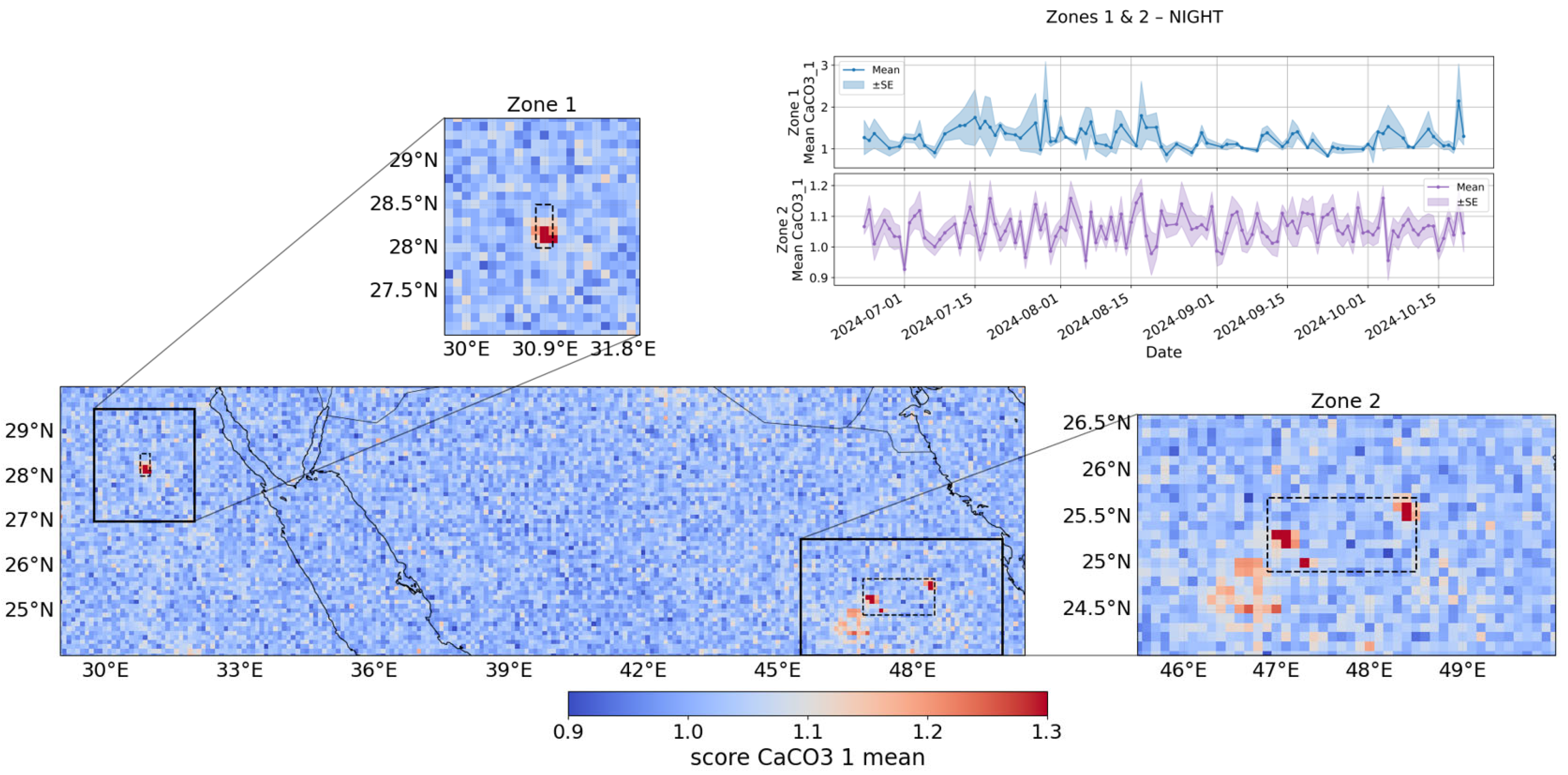
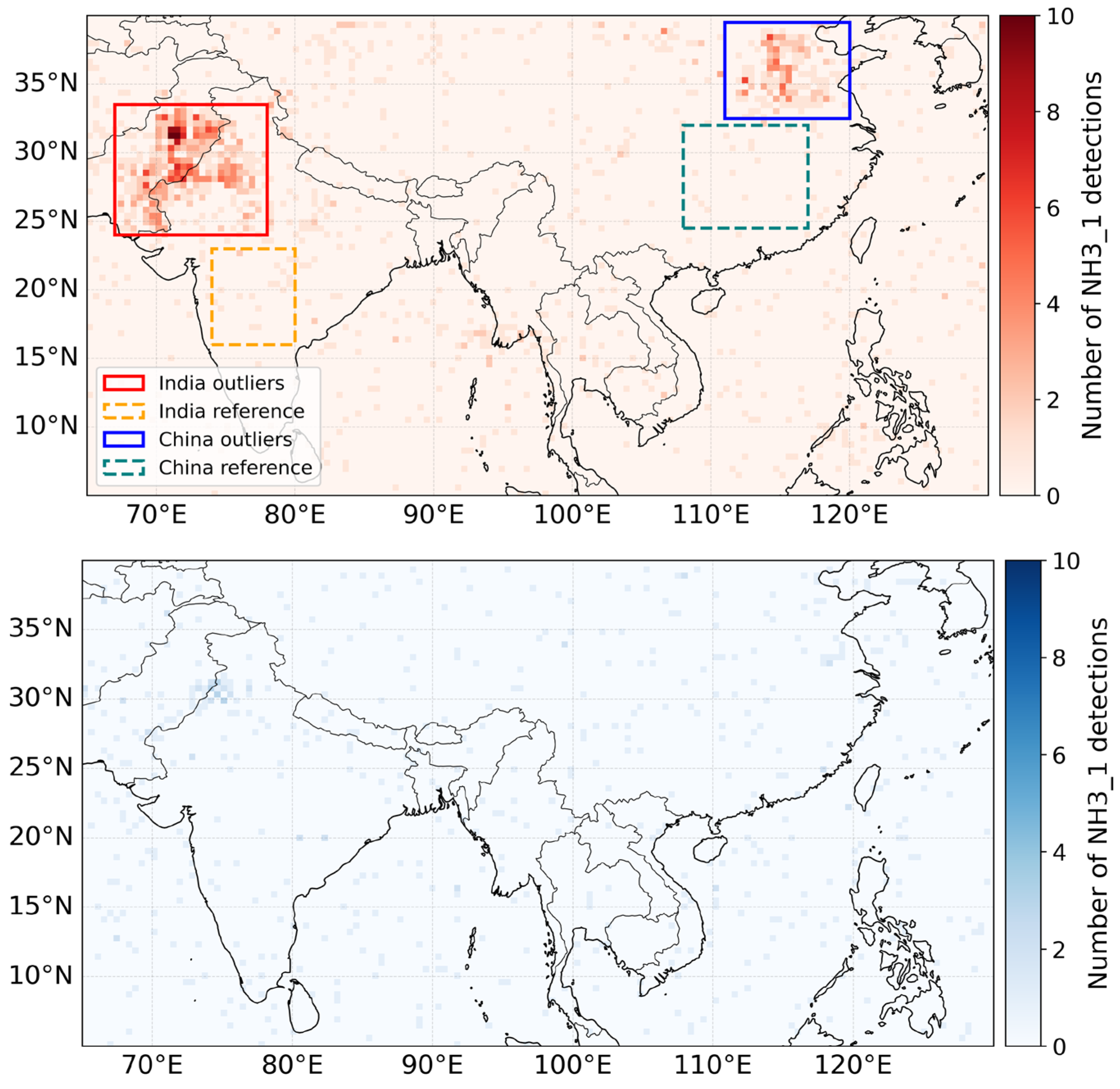
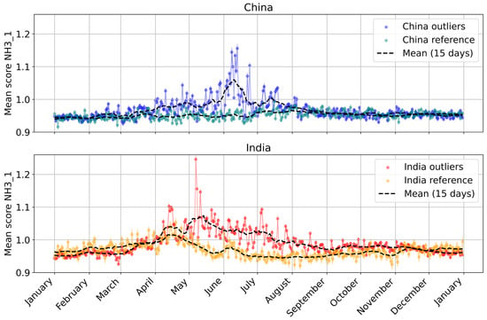
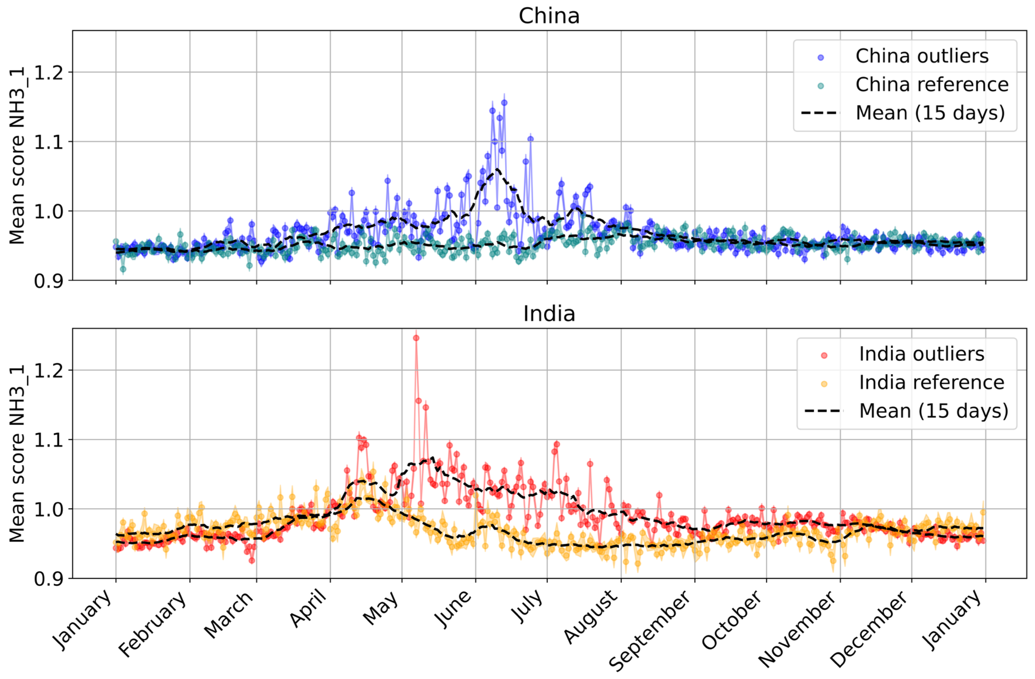
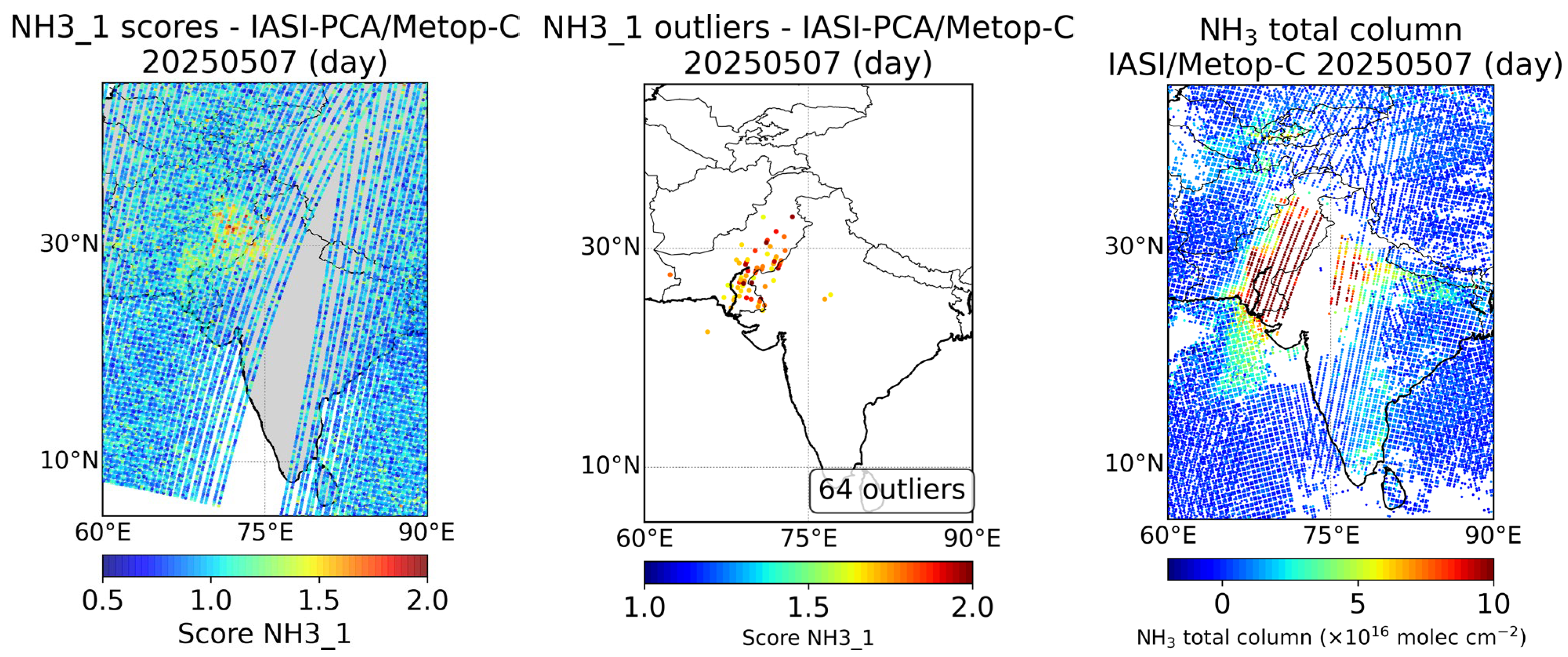
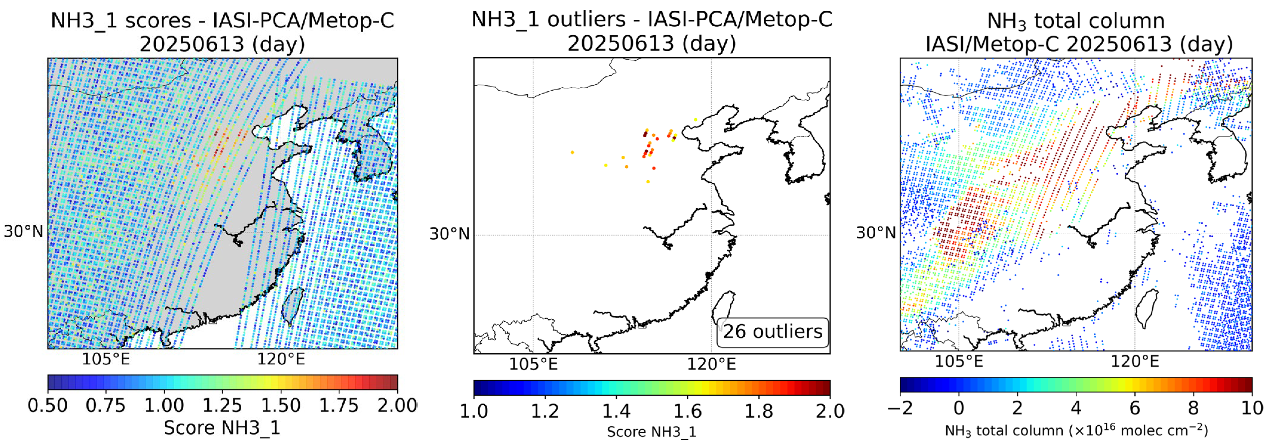
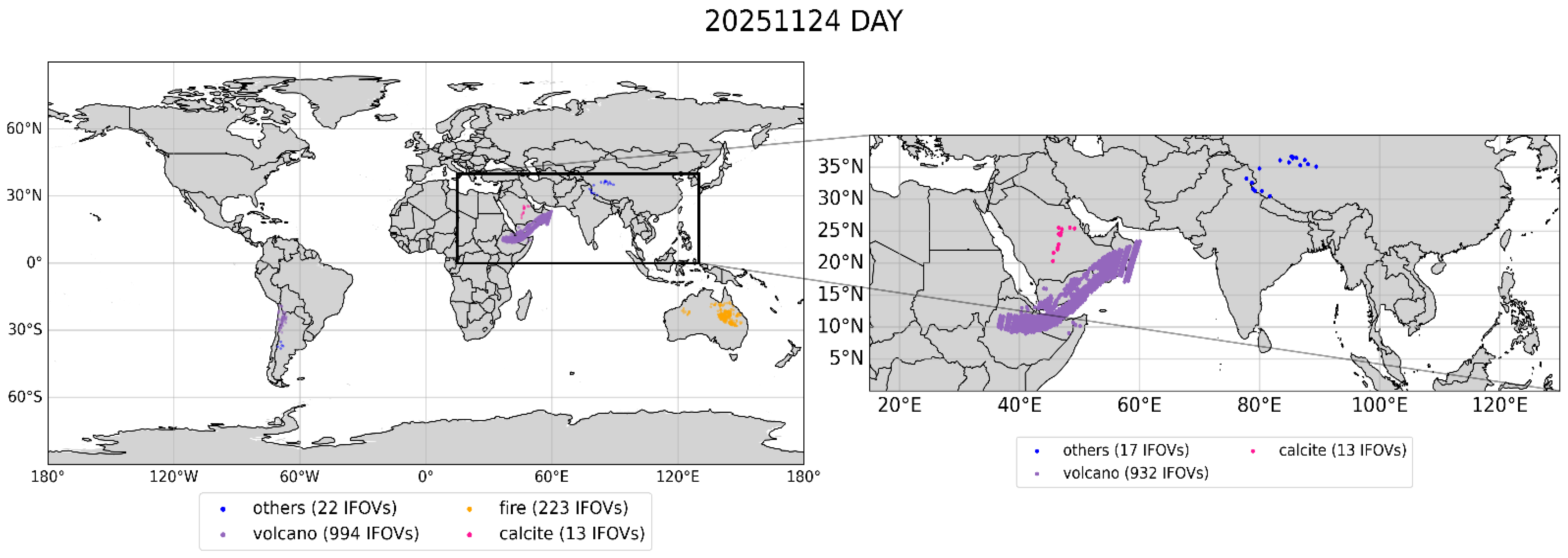
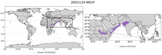
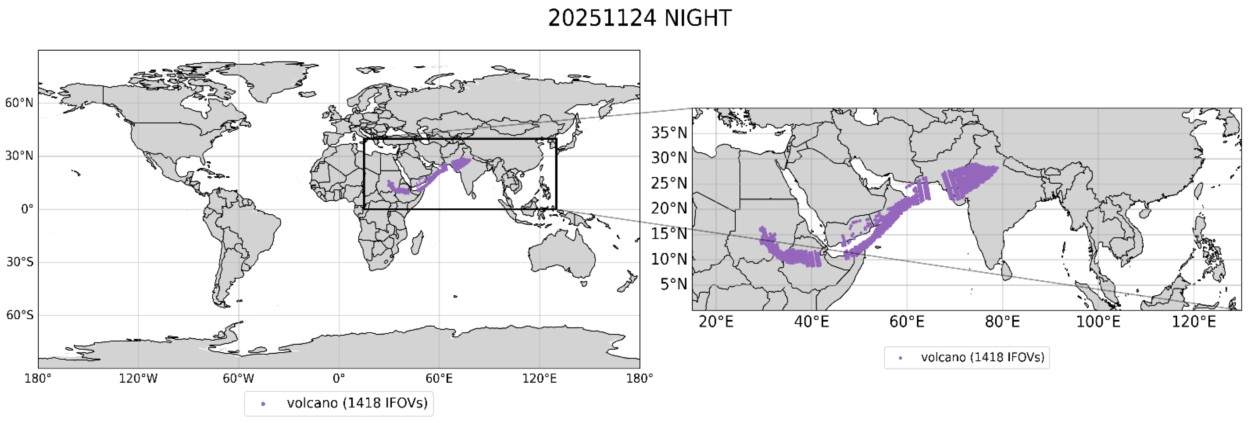

Disclaimer/Publisher’s Note: The statements, opinions and data contained in all publications are solely those of the individual author(s) and contributor(s) and not of MDPI and/or the editor(s). MDPI and/or the editor(s) disclaim responsibility for any injury to people or property resulting from any ideas, methods, instructions or products referred to in the content. |
© 2026 by the authors. Licensee MDPI, Basel, Switzerland. This article is an open access article distributed under the terms and conditions of the Creative Commons Attribution (CC BY) license.