


Highlights
What are the main findings?
- Multi-source remote sensing (TROPOMI, MLS, ERA5, SRTM) resolves the horizontal and vertical structure of the Tibetan Plateau ozone valley, with its core confined to the UTLS and tightly anchored to topography (anomaly–elevation slope −0.0035 DU m−1, R2 = 0.89).
- Interpretable XGBoost-SHAP attribution identifies topography and stratosphere–troposphere exchange as the dominant spatial controls (~58% of explained variance), with the South Asian High mainly modulating seasonal amplitude.
What are the implications of the main findings?
- The framework separates locally anchored topographic–thermodynamic forcing from large-scale circulation, reframing the ozone valley as a quasi-stationary climatic imprint.
- It provides a transferable approach for the refined utilization of multi-source satellite data over complex terrain.
Abstract
The Tibetan Plateau ozone valley is a prominent summertime ozone minimum in the Northern Hemisphere upper troposphere–lower stratosphere (UTLS), with implications for regional radiative balance and climate. Although previous studies emphasized large-scale circulation during the Asian summer monsoon, the contributions of local topographic and thermodynamic processes remain less well quantified, in part because most analyses rely on coarse-resolution data. Here we develop a refined multi-source remote sensing framework integrating high-resolution TROPOMI observations (total column ozone, NO2, and HCHO), Microwave Limb Sounder (MLS) ozone profiles, ERA5 reanalysis, and SRTM topography. Within a physically informed scheme, local factors are treated as pixel-level predictors and large-scale circulation as regional-mean background fields, complemented by interpretable machine-learning attribution (XGBoost-SHAP). The ozone valley exhibits a pronounced horizontal and vertical structure, with its core anomaly confined to the UTLS and spatially anchored to plateau topography. The covariability between the South Asian High (SAH) and ozone mainly reflects a shared response to thermal forcing, while circulation modulates its amplitude. Attribution shows that topography (~41%) and stratosphere–troposphere exchange (~16%) together dominate the spatial organization of the ozone minimum (~58% of the explained variance; anomaly–elevation slope −0.0035 DU m−1, R2 = 0.89), whereas large-scale circulation (~13%) mainly drives its seasonal amplification. Mechanistically, the elevated plateau and intense summer heating lift the tropopause, injecting ozone-poor tropospheric air into the stratospheric reservoir and thereby diluting its ozone content. Consequently, while topographic and thermodynamic factors dictate the spatial pattern of ozone, large-scale circulation primarily modulates its seasonal amplitude over complex terrain. The ozone valley thus represents a quasi-stationary climatic imprint, and our framework advances refined satellite-based atmospheric observation over complex terrain.
1. Introduction
In the extratropics, total column ozone (TCO) exhibits a pronounced meridional gradient governed by large-scale circulation, stratosphere–troposphere exchange (STE), and photochemical processes. Superimposed on this background pattern, however, a persistent summertime low-ozone region has long been observed over the Tibetan Plateau—the so-called “ozone valley”. First identified in Total Ozone Mapping Spectrometer (TOMS) observations in the early 1990s [1,2,3,4], this feature is characterized by TCO values approximately 10–15% lower than those at comparable latitudes over eastern China and adjacent oceanic regions. Subsequent analyses based on Ozone Monitoring Instrument (OMI), Microwave Limb Sounder (MLS), and reanalysis datasets have shown that the anomaly is most pronounced in the upper troposphere–lower stratosphere (UTLS), where ozone variability exerts a strong influence on regional radiative balance and climate processes [5,6]. In particular, Guo et al. [7] reported a distinctive double-core vertical structure, with a primary minimum in the UTLS and a weaker secondary minimum in the mid-stratosphere, suggesting deep coupling between surface forcing over the plateau and large-scale transport processes. This double-core structure has since been corroborated by inter-regional comparison with the ozone valley over North America [8], and recent satellite-based analyses have further confirmed its persistence and topographic anchoring [9]. Understanding its horizontal and vertical structure and maintenance mechanisms, therefore, represents a crucial step toward delineating the complex interactions within the Plateau’s atmosphere–terrain system and their broader climatic relevance.
Current understanding attributes the ozone valley primarily to dynamical rather than chemical controls. During boreal summer, the South Asian High (SAH) dominates circulation in the UTLS and strongly modulates STE over South and East Asia [10,11,12,13]. Acting as an elevated heat source, the Tibetan Plateau drives deep convection that lifts ozone-poor air from the lower troposphere into the UTLS, while the anticyclonic flow associated with the SAH inhibits the horizontal intrusion of ozone-rich air from surrounding regions. These processes collectively sustain the climatological ozone minimum over the plateau and, in some cases, influence ozone distributions extending into the middle stratosphere. Although chemical effects related to reduced production and enhanced loss under low pressure and strong radiation have been discussed [11], they are generally regarded as secondary contributors compared with transport-driven mechanisms.
Despite this progress, several aspects of the ozone valley remain poorly constrained. Most existing studies rely on satellite and reanalysis products with horizontal resolutions of ~50–100 km or coarser [7,8,9,11,12], which inevitably smooth steep topographic gradients and mesoscale thermal contrasts across the plateau. As a result, the ozone valley is often treated as a spatially coherent regional feature [1,2,3,4], with limited attention paid to its fine-scale heterogeneity. It therefore remains unclear to what extent its structure is shaped by local topographic and thermal forcing, versus imposed by background circulation variability and large-scale transport. Addressing this question requires observations capable of resolving kilometer-scale gradients and an analysis framework that can disentangle intertwined dynamical controls. This motivates the use of refined, high-resolution multi-source remote sensing data combined with an interpretable attribution framework.
The TROPOspheric Monitoring Instrument (TROPOMI) offers a new observational perspective on this problem. Its unprecedented horizontal resolution (~3.5 × 5.5 km2) and near-daily global coverage enable systematic mapping of ozone distributions over complex terrain at spatial scales that were previously inaccessible, supported by extensive geophysical validation and retrieval improvements of TROPOMI ozone products [14,15]. While vertical information remains primarily constrained by limb-viewing instruments and reanalysis products, TROPOMI provides critical leverage for examining how ozone anomalies are spatially anchored to topography, surface thermal patterns, and upper-tropospheric structure. These capabilities open the door to a more detailed and physically grounded characterization of the ozone valley. Beyond ozone, TROPOMI simultaneously retrieves NO2 and HCHO at comparable resolution, enabling photochemical processes to be characterized within the same high-resolution observational framework, as demonstrated in TROPOMI-based studies of ozone formation regimes [16].
At the same time, recent advances in physically interpretable machine learning [17,18,19] provide an opportunity to move beyond descriptive diagnostics toward structural attribution of complex atmospheric systems. Rather than treating the ozone valley as a circulation-driven anomaly, such approaches enable quantitative separation of locally anchored thermodynamic forcing from remotely forced dynamical modulation, while preserving physical interpretability. In regions of complex terrain such as the Tibetan Plateau, where surface heating, tropopause geometry, and large-scale circulation are tightly coupled, this separation is essential for clarifying the hierarchy of controlling mechanisms.
Here, we develop a refined multi-source atmospheric remote sensing diagnostic framework for the Tibetan Plateau ozone valley. The framework integrates high-resolution TROPOMI observations (total column ozone and the photochemical proxies NO2 and HCHO), MLS profile measurements, ERA5 reanalysis fields, and Shuttle Radar Topography Mission (SRTM) topography, harmonized through quality control into a physically consistent dataset. Rather than treating the ozone minimum solely as a circulation-driven anomaly and interpreting it qualitatively, we analyze spatially heterogeneous local factors at the pixel level while representing large-scale circulation as regional-mean background fields, and apply an interpretable attribution scheme that couples eXtreme Gradient Boosting (XGBoost) with SHapley Additive exPlanations (SHAP)—hereafter, XGBoost-SHAP—to rank their relative contributions. This refined, multi-source, and physically interpretable approach distinguishes locally anchored forcing from large-scale dynamical modulation and demonstrates how refinement and utilization of atmospheric remote sensing data can advance the observation and mechanistic understanding of UTLS ozone over complex terrain. This work therefore exemplifies the refinement and utilization of multi-source atmospheric remote sensing data—from high-resolution TROPOMI retrievals to MLS profiles and ERA5 fields—for advanced atmospheric observation over complex terrain.
2. Materials and Methods
2.1. Data Sources and Preprocessing
This study integrates multi-source satellite remote sensing data and atmospheric reanalysis products to analyze the spatiotemporal variability of TCO over the Tibetan Plateau and its surrounding regions (25–40°N, 70–110°E) from September 2018 to September 2025. The primary objective is to quantify the relative contributions of various driving factors to the formation of the ozone valley. The dataset includes ozone observations, meteorological dynamics, atmospheric chemistry, and topographical information, providing a comprehensive foundation for subsequent fine-structure diagnostics and multi-factor attribution analysis.
The core dataset for ozone observations combines complementary satellite products to characterize the ozone valley’s spatial and vertical distribution. The TCO data are sourced from the TROPOMI instrument on the Sentinel-5 Precursor satellite. The Level 3 offline (OFFL) product, with a spatial resolution of 3.5 km, provides monthly averages, which were processed using Google Earth Engine. TROPOMI’s high spatial resolution allows for the detailed characterization of the ozone valley’s fine-scale spatial structure, revealing its relationship with complex terrain. Vertical ozone profiles are obtained from the MLS version 5.0, Level 2 data, which cover 17 standard pressure levels from 15 to 316 hPa with a vertical resolution of approximately 2.5–3 km. Combining high-resolution TROPOMI total column ozone with MLS limb vertical profiles yields complementary horizontal detail and vertical structure for characterizing the ozone valley, consistent with the nadir–limb multi-sensor synergy strategy commonly discussed in tropospheric ozone satellite remote sensing [20,21]. Only data meeting quality control criteria (mass > 0.5 and status = 0) were retained, and the data were gridded to a resolution of 0.5° × 1° for monthly averages. The reliability of MLS ozone profiles over the region has been established through comparison with ozonesonde measurements near the South Asian High center [22]. These combined datasets enable concurrent analysis of the ozone valley’s total column characteristics and its vertical distribution within the UTLS.
Meteorological data are derived from the ECMWF ERA5 monthly reanalysis [23], with a horizontal resolution of 0.25° × 0.25°, accessed via the Copernicus Climate Data Store. The dataset includes key variables such as geopotential height at 200 hPa, which is used to characterize the intensity and spatial extent of the SAH. Additionally, temperature, horizontal wind components (zonal and meridional), and divergence at 200 hPa are employed to diagnose UTLS circulation patterns. Vertical velocity (ω) at 500 and 200 hPa, along with vertical profiles between 70 and 850 hPa, help characterize vertical motion. Potential vorticity (PV) at 100–300 hPa identifies stratospheric intrusions, while PV contours at 30–450 hPa based on the 2 potential vorticity units (PVU) criterion determine the dynamic tropopause height. Surface and boundary layer variables—including sensible heat flux, convective available potential energy (CAPE), boundary layer height, convective precipitation, surface downwelling shortwave radiation, total cloud cover, and total column water vapor—represent local thermal forcing and convective activity for use in the attribution analysis.
Additional tropospheric trace gas column densities, specifically NO2 and HCHO, are obtained from TROPOMI Level 3 products at a 3.5 km resolution. NO2 serves as an indicator of anthropogenic nitrogen oxide emissions, and HCHO serves as a proxy for volatile organic compound oxidation, facilitating an assessment of photochemical contributions to the ozone budget. Topographic data from the SRTM version 4 [24], at approximately 90 m (3 arc-second) resolution, are used to define baseline topographic constraints on atmospheric column thickness over the Tibetan Plateau, facilitating detailed terrain–ozone interaction analysis using high-resolution TROPOMI data.
Data preprocessing involved the aggregation of daily TROPOMI observations into monthly mean products by averaging all valid data within each month. Observations with unphysical values were flagged and excluded. Missing values were handled by direct exclusion rather than interpolation to minimize the introduction of additional uncertainty. For attribution analysis, only grid points with valid observations across all driving factors were retained, ensuring matrix completeness. ERA5 geopotential height data were converted from m2 s−2 to geopotential meters (gpm) by dividing by 9.80665 m/s2. All meteorological fields were clipped to the study domain. Because the analysis combines variables with very different native resolutions and formats, all predictors were harmonized onto a common analysis grid prior to attribution. Spatially resolved local fields—TROPOMI total column ozone, NO2 and HCHO, the SRTM elevation, the 2 PVU tropopause pressure, and the ERA5 surface and pressure-level variables—were regridded to the target grid and retained at the pixel level, whereas large-scale (non-local) circulation indices were computed as regional means over prescribed domains and applied as spatially uniform background fields. This explicit separation of pixel-level local predictors from regional-mean non-local indices is the methodological basis for distinguishing spatially anchored forcing from large-scale dynamical modulation in the subsequent attribution.
2.2. Diagnostic Indices and Methods
The intensity of the SAH is characterized by the regional mean 200 hPa geopotential height during boreal summer (June–August) over the Tibetan Plateau and adjacent regions (25–40°N, 70–110°E). The resulting South Asian High Intensity Index (SAHI) provides a spatially representative measure that suppresses local extremes. For the study period (2018–2025), the climatological summer mean SAHI is 12,522.9 with an interannual standard deviation of 14.3, consistent with long-term climatological statistics reported by Wei et al. [25], indicating that the selected period adequately captures representative SAH variability.
To delineate the spatial extent of the SAH, we define the SAH core region using the 75th percentile of the summer 200 hPa geopotential height distribution (12,585 gpm), with grid points exceeding this threshold classified as part of the SAH core. This threshold closely matches climatological ridge positions reported in previous studies and is further validated through sensitivity tests using percentile thresholds ranging from 70% to 85% (12,578–12,598 gpm), which yield consistent seasonal evolution patterns. The SAH center is identified using a weighted centroid method, with weights proportional to the geopotential height exceeding the threshold, enabling quantitative diagnosis of its spatial displacement.
The spatial characteristics of the ozone valley are quantified using two complementary metrics. The Ozone Zonal Anomaly (ZA) is defined as the deviation of the ozone column concentration at each grid point from the zonal mean at the corresponding latitude. The ozone valley intensity index (TOVI) is calculated as the area-weighted mean of negative ZA values within the study domain, with cosine-latitude weighting applied to account for grid-cell area variation. The ozone valley center is likewise determined using a weighted centroid approach, with weights proportional to the absolute magnitude of negative ozone anomalies, ensuring methodological consistency with the SAH center diagnostics.
STE is characterized using the dynamical tropopause, defined by the 2 PVU isosurface [26], which provides a more physically meaningful representation of the exchange interface over complex terrain than the thermal tropopause [27]. Tropopause pressure is converted to geometric height using a standard pressure–height relationship. The zonal anomaly of tropopause height is computed as the deviation from the zonal mean at each latitude to quantify regional-scale tropopause uplift over the Tibetan Plateau.
Based on these indices, the spatiotemporal relationship between the SAH and the ozone valley is diagnosed from spatial, intraseasonal, and interannual perspectives. Spatial correspondence is evaluated by overlaying the SAH boundary (12,585 gpm contour at 200 hPa) on ozone zonal anomaly fields for individual months from May to October. Temporal covariability is assessed using Pearson and Spearman correlation analyses between monthly SAHI and TOVI during the active season (June–September), considering lead–lag relationships within a ±2-month window. On the interannual scale, linear regression is applied to the summer-mean positions of the SAH and ozone valley centers to quantify their co-migration characteristics.
To further examine the role of vertical processes, longitude–pressure cross-sections along 32°N are constructed using MLS ozone profiles and ERA5 reanalysis data, comparing summer and winter distributions of ozone mixing ratio, vertical velocity, and potential temperature. The contribution of surface thermal forcing is evaluated using partial correlation analysis, bootstrap resampling [28], and Granger causality testing [29] applied to summer monthly time series, enabling assessment of both statistical robustness and temporal precedence between sensible heat flux and vertical motion.
2.3. Multi-Factor Attribution Framework
To quantify the relative contributions of multiple factors to the spatial distribution of the ozone valley, we employ a machine learning-based multi-factor attribution framework. A central design of our attribution framework is the explicit distinction between local and non-local factors: local factors are analyzed as spatially heterogeneous, pixel-level predictors, whereas non-local large-scale circulation factors are represented as regional-mean time series, so that their influence is evaluated without imposing artificial spatial structure. The XGBoost model [30] is used to fit the spatiotemporal distribution of the ozone valley, with the SHapley Additive exPlanations (SHAP) method [31] applied for post-model interpretation. The machine-learning component is not used to replace physical reasoning but as a physically informed, interpretable tool to quantify and rank the relative importance of the multi-source predictors; all attribution results are cross-checked against expected physical signs and four reliability tests. Here, “physically informed” does not imply hard physical constraints imposed on the learning algorithm; it refers to four physics-based safeguards: (i) predictor selection guided by known ozone-valley mechanisms; (ii) explicit separation of pixel-level local predictors from regional-mean non-local circulation indices; (iii) verification that SHAP contribution signs are consistent with expected physical mechanisms; and (iv) removal of collinear variables via VIF.
Factor selection follows a physically informed approach, distinguishing between local and non-local factors. Preliminary screening identifies five key categories of processes influencing the ozone valley: (1) geometric effects (topographic constraints on atmospheric column thickness), (2) thermodynamic and dynamic processes (including thermal forcing and vertical motion), (3) STE, (4) large-scale circulation modulation (SAH and jet stream dynamics), and (5) photochemical processes (involving precursor concentrations and radiation). Variance Inflation Factor (VIF) analysis is used to eliminate highly collinear variables, resulting in a final set of 24 factors with clear physical relevance (Table A2).
These factors are divided into local and non-local groups. Local factors exhibit significant spatial variability and include Digital Elevation Model (DEM), thermal forcing (sensible heat flux, CAPE, boundary layer height), dynamics (vertical velocity, convective precipitation), STE (tropopause pressure, 200 hPa PV), chemistry (NO2, HCHO), and radiation (total cloud cover, surface downwelling shortwave radiation). Non-local factors include large-scale circulation components such as SAH intensity, jet stream dynamics, and 200 hPa wind patterns. These non-local factors are represented as regional mean time series for comparison with local factors in the unified attribution analysis framework.
The XGBoost model is configured with the following parameters to balance model complexity and generalization: 100 iterations, a min_child_weight of 10, a maximum tree depth of 4, a learning rate of 0.1, L1 regularization (reg_alpha) of 0.5, and L2 regularization (reg_lambda) of 2.0, with 80% subsampling. The model’s performance is evaluated using 5-fold cross-validation, with training and validation R2 values of 0.958 and 0.953, respectively, demonstrating strong generalization capability.
The attribution results are verified through four reliability tests: (1) sensitivity analysis in which key factors (e.g., DEM) are withheld to assess the stability of the factor ranking and the degree of collinearity-driven redistribution among predictors, (2) spatial variation coefficient analysis (CV) to evaluate the physical significance of factors with low spatial variability, (3) physical consistency tests to ensure that SHAP values align with expected physical mechanisms, and (4) SHAP contribution stability is assessed through 200 bootstrap iterations [28], in which the training set is resampled with replacement and the full XGBoost–SHAP pipeline is re-executed. The bootstrap mean, standard deviation, and 95% confidence interval of each factor’s contribution are reported in Table 1. These tests confirm the robustness and physical interpretability of the attribution results.
Table 1.
SHAP-based attribution and sensitivity analysis of 24 driving factors contributing to Tibetan Plateau ozone valley (TPOV) formation.
3. Results
3.1. Horizontal and Vertical Structure of the Ozone Valley
3.1.1. Horizontal Distribution of Total Column Ozone and Seasonal Evolution
Leveraging the ~3.5 km horizontal resolution of TROPOMI, we first examine the spatiotemporal characteristics of TCO over the Tibetan Plateau and its broader mid-latitude surroundings (20–50°N, 40–140°E) using multi-year observations from September 2018 to September 2025 (Figure A1). TCO exhibits a pronounced seasonal cycle, with maximum values in winter and early spring and a minimum in summer. Wintertime TCO exceeds 340 Dobson Units (DU) over much of the Plateau, whereas summer values decrease to approximately 260 DU. Throughout the year, TCO displays a strong meridional gradient, increasing toward higher latitudes. Against this large-scale background, the Tibetan Plateau stands out as a distinct low-ozone region during spring and summer, forming the deepest midlatitude ozone minimum in the Northern Hemisphere.
Because the strong latitudinal gradient obscures plateau-specific signals, we remove the zonal-mean background by calculating ZA, defined as deviations from the latitude-band mean. The ZA fields isolate the regional ozone deficit associated with the Plateau and reveal the detailed seasonal evolution of the ozone valley (Figure 1).
Figure 1.
Multi-year mean monthly zonal anomalies (ZA, DU) of total column ozone over the Tibetan Plateau and surrounding mid-latitude region (20–50°N, 40–140°E; September 2018–September 2025). Panels (a–l) correspond to January through December.
Figure 1 presents the spatial pattern of the ZA, which clearly delineates the seasonal evolution of the ozone valley. In winter (DJF), the Plateau exhibits a pronounced north–south dipole, with positive anomalies over the central–northern Plateau and weak negative anomalies confined to the southern margin. In spring (MAM), negative anomalies intensify rapidly and expand northward, forming a basin-wide ozone valley that peaks in May. In summer (JJA), the ozone valley persists as a quasi-stationary broad minimum centered over the central–western Plateau, although its magnitude weakens slightly relative to the May maximum. In autumn (SON), positive anomalies re-emerge in the north, and the ozone valley weakens and retreats southward toward the winter configuration. Together, these results indicate that the Tibetan Plateau ozone valley is a persistent year-round feature with strong seasonal modulation rather than a purely summer phenomenon. The frequency and intensity of extreme ozone-valley events have also been documented from long-term reanalysis [32].
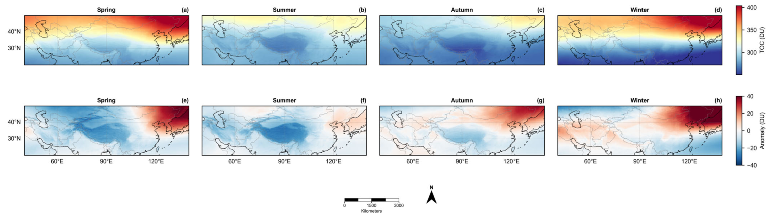
To facilitate comparison with previous studies, we construct seasonal composites of TCO and ZA (Figure A2). Summer exhibits the broadest spatial coverage and the strongest ozone depletion, with ZA over the plateau interior generally below −20 DU (about 47% of the plateau domain) and locally reaching approximately −34 DU. Winter shows the weakest and most confined anomalies (domain-mean ZA ≈ −23 DU), while spring and autumn serve as transitional seasons. Although May represents the strongest monthly anomaly, the seasonal composites indicate that summer dominates in terms of persistence rather than peak intensity. This distinction motivates our focus on the boreal summer (JJA) broad-valley state in subsequent mechanistic analyses.
To assess whether the horizontal extent of the summer ozone valley is modulated by topography, we constructed seven-summer mean (June–August, 2019–2025) ZA maps at the native TROPOMI resolution (~3.5 km), overlaid with 3000 m and 5000 m elevation contours derived from the 90 m SRTM DEM (Figure 2a). The kilometer-scale ZA field exhibits progressively deepening ozone depletion toward the plateau interior, spatially aligned with increasing elevation. Mean ZA values transition from approximately −10 DU below 1000 m to −17 DU between 1000 and 3000 m, further deepening to −25 DU between 3000 and 5000 m, and reaching −27 DU above 5000 m. Pixel-level regression of ZA against surface elevation (Figure 2b; n = 528,022) yields a slope of −0.0035 DU m−1 (R2 = 0.89, p < 0.001), indicating a strong statistical dependence. Below ~6000 m, 500 m binned means closely follow the regression relationship. Deviations at higher elevations likely reflect reduced sample size (n = 948 above 6000 m) and a possible transition toward greater free-tropospheric influence.
Figure 2.
Spatial correspondence between the summertime ozone valley and plateau topography. (a) Seven-summer mean (JJA, 2019–2025) ozone zonal anomaly (DU) from TROPOMI (~3.5 km), with elevation contours at 3000 and 5000 m a.s.l. derived from the SRTM ~90 m (3 arc-second) DEM interpolated to a 3 km grid for smoother contouring; (b) pixel-level scatter plot of elevation versus zonal anomaly (n = 528,022), with 500 m binned means ± 1σ (black dots) and ordinary least-squares fit (red line; slope = −0.0035 DU m−1, R2 = 0.89, p < 0.001).
The observed elevation dependence is consistent with previously proposed elevation-related ozone deficit mechanisms based on high-altitude station measurements (e.g., [33]). By providing spatially continuous kilometer-scale retrievals, our analysis extends station-based evidence across the entire plateau region and highlights a robust coupling between the summer ozone valley and the topographic envelope. The dynamical and vertical mechanisms underlying this coupling are examined in the following sections.
3.1.2. Vertical Distribution of Ozone Mixing Ratio and Seasonal Variation
Before analyzing the MLS profiles, we cross-checked the two ozone products by comparing TROPOMI total column ozone with the MLS-integrated partial column over the plateau (Figure 3); the two are highly consistent (r = +0.92 for all months and r = +0.91 for JJA, p < 0.001), confirming that the nadir and limb measurements depict a mutually consistent ozone field.
Figure 3.
Comparison between TROPOMI total column ozone (TCO) and the MLS-integrated partial ozone column over the Tibetan Plateau (September 2018–September 2025). (a) Monthly co-variation in TROPOMI TCO (blue) and the MLS 316–15 hPa partial column (red); (b) scatter of TROPOMI TCO versus the MLS partial column (r = 0.92, p < 0.001, n = 85); red points denote boreal-summer (JJA) months, and the black dashed line shows the ordinary-least-squares linear fit.
While TCO and ZA characterize the horizontal structure of the ozone valley, they do not constrain its vertical extent. To extend the refined horizontal characterization into the vertical dimension, we analyze ozone mixing-ratio profiles from Aura MLS and their zonal anomalies to diagnose the altitude range and seasonal evolution of ozone depletion (Figure 4).
Figure 4.
Seasonal variations in ozone vertical structure and zonal anomalies over the Tibetan Plateau. (a–d) Mean vertical ozone profiles in winter (DJF), spring (MAM), summer (JJA), and autumn (SON); (e–h) corresponding zonal anomalies relative to the 25–40°N latitude band. Shading denotes ±1 standard deviation. Red downward triangles in (e–h) mark the pressure level of the maximum negative zonal anomaly (i.e., the core of the ozone valley) in each season.
Seasonal mean profiles (Figure 4a–d) show low ozone concentrations in the troposphere and a sharp increase across the tropopause into the stratosphere. In winter, profiles below ~300 hPa are relatively smooth, with steadily increasing ozone above ~200 hPa and no distinct low-ozone layer. In spring, the rising tropopause is accompanied by a weakened vertical gradient in the UTLS, indicating the onset of ozone dilution. In summer, a pronounced low-ozone layer develops between ~150 and 100 hPa, with mixing ratios reduced to ~0.10–0.15 ppmv, while the chemical tropopause rises to ~70–80 hPa, reflecting strong upward transport into the lower stratosphere. In autumn, this structure relaxes, and ozone concentrations recover toward the winter profile.
To isolate Plateau-specific signals from the background latitudinal gradient, we compute zonal anomalies of the vertical profiles (Figure 4e–h). Negative anomalies are confined primarily to the UTLS and exhibit strong seasonality. In winter, anomalies are near zero throughout the UTLS, indicating little net ozone deficit. In spring, negative anomalies emerge between ~260 and 30 hPa and peak near ~80–70 hPa (−0.15 to −0.20 ppmv). In summer, anomalies intensify and extend vertically from ~215 to 15 hPa, covering nearly the entire UTLS and lower stratosphere, with weak but persistent deficits even above ~40 hPa (−0.01 to −0.05 ppmv). In autumn, negative anomalies retreat to ~178–56 hPa and weaken to −0.09 to −0.10 ppmv. Integrating the zonal anomaly profiles between 316 and 15 hPa yields net column anomalies of −0.17 ppmv in summer, −0.09 ppmv in spring, +0.03 ppmv in autumn (near balance), and +0.12 ppmv in winter. The wintertime positive anomaly originates mainly from the middle and upper stratosphere (56–15 hPa), accompanied by weak negative anomalies in the lower stratosphere, indicating a more vertically complex and variable structure than in other seasons.
Together, the vertical profile and zonal anomaly analyses indicate that the core of the Tibetan Plateau ozone valley is centered near ~70 hPa, strengthens rapidly in spring, peaks in summer, and weakens in autumn. Summer depletion is not only strongest in magnitude but also extends upward into the middle stratosphere. Although previous studies have attributed this seasonal pattern primarily to dynamical transport associated with the SAH, the detailed spatial and temporal correspondence between these features requires further examination, which is addressed in the following sections.
3.2. Spatiotemporal Configuration and Dynamic Covariation Between the South Asian High and the Ozone Valley
The SAH has long been considered a key circulation feature associated with the summertime ozone valley [34]; here we use the spatially refined satellite and reanalysis fields to re-examine their relationship at finer spatial and temporal scales. However, its precise relationship with the ozone valley at finer spatial and temporal scales remains unclear. In this section, we examine the spatiotemporal configuration and dynamic covariation between the SAH and the ozone valley from three perspectives: spatial alignment, intraseasonal variability, and interannual displacement.
Figure 5 shows the evolution of the SAH and ozone valley from May to October. During May–June, the SAH starts to form but does not yet fully cover the Plateau. By September–October, it weakens and retreats southward. In July–August, the SAH reaches its mature phase, but the centers of the SAH and the ozone valley do not coincide. In July, the ozone valley center is located near 89.4°E, 33.3°N, whereas the SAH center is located at ~82.5°E, 29.0°N, showing offsets of ~7° longitude and ~4° latitude. A similar offset is observed in August. Despite this, the ozone valley remains within the broader SAH-influenced region, suggesting that while the SAH provides a favorable large-scale dynamical background, the precise positioning of the ozone valley is modulated by regional processes.
Figure 5.
Monthly spatial co-evolution of the South Asian High (SAH) and the ozone valley for (a) May, (b) June, (c) July, (d) August, (e) September and (f) October. Shading denotes ozone zonal anomalies (DU); yellow stars mark the ozone-valley centre. Red contours and red stars (panels c–d only) indicate the SAH boundary (200-hPa geopotential height ≥ 12,585 gpm) and the SAH centre, respectively; a closed SAH contour meeting this threshold is present mainly in midsummer.
We further compare the seasonal cycles of the SAH and ozone valley. Ozone depletion peaks in May, while the SAH reaches maximum intensity in July–August (Figure 6a), suggesting that their evolution is not fully synchronized. Pearson correlations (Figure 6b) show weak contemporaneous correlation (r = 0.19; p = 0.31), indicating that month-to-month fluctuations in the ozone valley do not track those of the SAH. However, significant positive correlations emerge when ozone leads by one month (r = 0.72, p < 0.001), while negative correlations occur when the SAH leads by one month (r = −0.66, p < 0.001), implying that intraseasonal variations in the ozone valley tend to precede changes in SAH intensity (Table A1).
Figure 6.
Seasonal to interannual relationships between the South Asian High (SAH) and the ozone valley. (a) Seasonal cycles; (b) lagged correlations; (c) covariation of center longitude; (d) covariation of center latitude. Shading in (a) denotes ±1 standard deviation. In (b), horizontal dashed lines mark |r| = 0.3 as a reference for moderate correlation; bar colours indicate statistical significance (p < 0.05).
At the interannual scale, we find no significant correlation in the longitudinal displacement of the SAH and ozone valley (R2 = 0.249, p = 0.25, Figure 6c). In contrast, the latitudinal positions show a significant positive correlation (R2 = 0.706, p = 0.018; Figure 6d), suggesting that northward shifts in the SAH are associated with a slight northward displacement of the ozone valley (~1° latitude). However, the ozone valley’s meridional migration is strongly constrained by regional processes.
These results indicate that while the SAH plays an important role in setting the large-scale dynamical environment for ozone depletion, the precise location and variability of the ozone valley are also influenced by local factors, such as topography and thermal forcing, which we explore further in the following sections.
3.3. Local Vertical Structure and Thermal Forcing Verification
Previous analyses focused on the relationship between the SAH and the ozone valley from a large-scale circulation perspective. While SAH-driven anticyclonic transport and horizontal confinement have been widely regarded as key mechanisms shaping the ozone valley [2,12,35], large-scale circulation alone cannot fully explain the spatial anchoring or seasonal variability of ozone minima over the Tibetan Plateau. Recent studies suggest that strong summertime surface heating induces deep local ascent, which may directly drive ozone depletion in the UTLS [36,37]. Here, we examine the vertical structure of ozone, vertical motion, and tropopause height, and disentangle the independent contributions of surface thermal forcing and the SAH using statistical and causal analyses.
Combining MLS ozone profiles with ERA5 vertical velocity, temperature, and tropopause diagnostics, we examine the vertical structure of ozone and disentangle the contributions of surface thermal forcing and the SAH. Longitude–pressure cross-sections along 32°N illustrate the vertical coupling between ozone, vertical velocity, and temperature (Figure 7). In summer, a pronounced UTLS ozone minimum (<0.6 ppmv) occurs between 75°E and 95°E over the Plateau, coinciding with persistent upward motion and an upward displacement of temperature contours. This indicates that the dynamical tropopause rises near 100 hPa, and sustained ascent lifts low-ozone tropospheric air into the UTLS, directly regulating ozone distribution. By contrast, in winter, vertical velocity alternates between ascent and descent associated with wave-like disturbances, ozone concentrations are higher and more uniform, and the tropopause descends. The strong seasonal contrast highlights continuous summertime ascent over the Plateau as a primary driver of tropopause uplift and UTLS ozone depletion, controlling the seasonal cycle of the ozone valley.
Figure 7.
Summer–winter contrasts in vertical structure along 32°N over the Tibetan Plateau. (a,d) Ozone mixing ratio; (b,e) vertical velocity; (c,f) potential temperature. Left column: summer (JJA); right column: winter (DJF). Black solid lines indicate the dynamical tropopause (2 PVU).
The spatial pattern of tropopause height further supports this mechanism (Figure 8), consistent with the documented spatiotemporal variability of the tropopause over the plateau [38]. Absolute summer tropopause heights exceed 14 km and reach 15–16 km over the western Plateau (Figure 8a). After removing the zonal mean at each latitude, positive anomalies of +1.66 km are found over the Plateau core (28–36°N, 80–100°E), spatially coincident with the strongest ascent and lowest ozone (Figure 8b). Tropopause height anomalies are significantly negatively correlated with ozone anomalies (r = −0.221, p < 0.001; Figure 8c), consistent with a mechanism in which thermally driven ascent lifts the tropopause, replacing UTLS air with low-ozone tropospheric air, thereby intensifying the ozone valley.
Figure 8.
Summer tropopause height characteristics over the Tibetan Plateau and their relationship with ozone anomalies. (a) Spatial distribution of tropopause height; (b) zonal anomalies of tropopause height; (c) scatter relationship between tropopause height anomalies and ozone zonal anomalies.
To quantify the relative influence of surface heating and the SAH on vertical motion, we apply partial correlation, bootstrap resampling, and Granger causality tests to summer monthly time series over the Plateau (2018–2025; n = 24; Figure 9). After controlling for topography, the correlation between surface sensible heat flux and vertical velocity strengthened from −0.39 (p = 0.059) to −0.66 (p < 0.001) and remained significant when SAH intensity was further controlled (r = −0.51, p = 0.010). In contrast, although the SAH–vertical velocity correlation became significant after removing topographic effects (r = −0.49, p = 0.017), it vanished once surface sensible heat was accounted for (r = −0.13, p = 0.544), indicating that the apparent SAH influence is largely mediated by thermal forcing rather than representing an independent driver. Bootstrap resampling confirms the robustness of the surface heating effect, with the 95% confidence interval excluding zero, whereas that of the SAH spans zero. Granger causality tests further show that sensible heat flux leads vertical velocity by one month (p < 0.001), while the SAH exhibits predictive skill only at two- to three-month lags, consistent with a delayed, indirect response to Plateau heating rather than direct dynamical forcing (Figure 9c,d).
Figure 9.
Evidence supporting thermal forcing as the primary driver of vertical motion. (a) Partial correlation coefficients; (b) bootstrap 95% confidence intervals; (c) Granger causality tests; (d) lagged correlation analysis In (a), * and ** indicate statistical significance at p < 0.05 and p < 0.01, respectively.
Taken together, these observations and statistical diagnostics demonstrate that surface thermal forcing is the dominant driver of vertical motion over the Plateau on monthly timescales. While the SAH contributes to the large-scale dynamical background favoring ozone confinement and upward transport, the direct regulation of UTLS ozone occurs through thermally induced ascent and tropopause uplift. The ozone valley therefore emerges from the coordinated action of large-scale circulation, regional thermal forcing, and vertical dynamical adjustment. Future work extending the temporal record and incorporating model-based attribution frameworks will allow further quantification of the relative contributions of these processes.
3.4. Factor Separation-Based Quantitative Attribution Results
The Tibetan Plateau ozone valley arises from coupled influences of topography, thermally driven vertical adjustment, STE, large-scale circulation, and photochemical loss (Figure 10) [39]. Because these processes co-vary in space and time, we implemented a unified attribution framework to quantify their relative contributions while distinguishing local structural controls from non-local dynamical modulation. In this framework, local factors are evaluated as spatially resolved, pixel-level predictors, whereas non-local circulation indices are introduced as regional-mean background fields so that structural and dynamical controls can be assessed simultaneously without imposing artificial spatial structure.
Figure 10.
Conceptual schematic of the physical mechanisms governing the formation of the Tibetan Plateau ozone valley, including: (1) geometric column thinning; (2) surface thermal uplift; (3) tropopause elevation and weakened stratosphere–troposphere exchange; (4) confinement by the South Asian High and subtropical jet; (5) chemical loss processes. Relative quantitative contributions are summarized in Table 1.
We first classify 24 physically interpretable factors into five major categories: geometric effects of topography and column shortening; thermodynamic and dynamical processes driven by surface sensible heating and vertical motion; STE regulating vertical ozone redistribution; large-scale circulation modulation dominated by SAH and jet stream blocking; and photochemical loss influenced by radiation, water vapor, and precursor concentrations. Local variables were treated as spatially resolved predictors, whereas non-local circulation indices were introduced as spatially uniform background fields, allowing simultaneous evaluation of structural and dynamical controls.
The optimized XGBoost model reproduces the observed ozone distribution with high skill (five-fold cross-validation R2 ≈ 0.95), indicating that the selected predictors capture the dominant spatial variability. SHAP-based attribution (Table 1) reveals a clear hierarchy of influence. This quantitative, physically interpretable ranking of multi-source predictors—rather than a qualitative description—is a central contribution of this study. The elevation-associated term ranks first, explaining approximately 41% of the modeled variance. We caution that this value should not be read as a purely geometric effect: because surface elevation covaries with the geometric shortening of the overhead air column and, at the same time, with intense surface heating and an elevated tropopause, its attributed importance combines geometric and thermodynamic–dynamical contributions that cannot be separated using total-column data alone.
STE-related indicators collectively account for about 16% of the explained variance, primarily through tropopause pressure and 200 hPa potential vorticity, suggesting the role of large-scale vertical redistribution processes. Photochemical indicators account for approximately 14%, with water vapor and precursor variability associated with enhanced ozone loss, particularly under moist conditions. Large-scale circulation factors contribute roughly 13%, likely through modulation of horizontal transport and dynamical confinement. We further note a more fundamental limitation: the available NO2 and HCHO retrievals are total-column quantities, and boundary-layer- or UTLS-specific partial columns cannot be obtained; their attributed contribution therefore reflects a statistical association with column-integrated photochemical conditions rather than direct evidence of in situ ozone loss within the UTLS valley core, and should be interpreted with corresponding caution. The strong statistical entanglement among co-located structural, thermodynamic, and dynamical predictors means that the geometric and thermodynamic–dynamical contributions of the elevation term cannot be uniquely separated within the model; we therefore interpret it as an integrated structural control rather than a pure geometric effect. SHAP contribution signs are physically consistent: higher elevation corresponds to lower ozone concentrations, elevated tropopause levels are associated with reduced UTLS ozone influence, and increased water vapor favors chemical depletion. Bootstrap resampling (200 realizations) confirms the robustness of the identified hierarchy. Elevation ranked first in all realizations, with a baseline contribution of 41.5% and a bootstrap mean of 39.3 ± 3.3% (95% confidence interval: 30.8–43.4%), and the top-five ranking order remained unchanged. These results indicate that the dominance of structural controls is not sensitive to sampling variability. The temporal role of circulation exhibits scale dependence. At seasonal scales, ozone valley intensity co-varies with circulation indices partly due to common solar forcing. At intra-seasonal and interannual scales, correlations weaken, suggesting that circulation primarily modulates background transport conditions rather than initiating ozone depletion (Table A3).
Overall, structural controls linked to topography and STE dominate the spatial configuration of the ozone valley (~58% of explained variance), while circulation and photochemical processes provide secondary modulation. These percentages reflect relative explanatory strength within the statistical framework rather than direct physical partitioning, but they consistently indicate that the ozone valley is fundamentally anchored by structural and thermodynamic constraints.
4. Discussion
4.1. Beyond Circulation: Topographic and Thermal Controls
By integrating high-resolution TROPOMI TCO, MLS vertical ozone profiles, and ERA5 reanalysis, this study refines the physical interpretation of the Tibetan Plateau ozone valley. This refined integration of multi-source satellite and reanalysis observations is what makes it possible to separate spatially fixed structural controls from temporally varying circulation modulation. Previous work has emphasized the role of large-scale circulation, particularly vertical transport and horizontal confinement associated with the SAH. Our results extend this framework by showing that the ozone valley’s spatial structure is anchored to plateau topography and thermally driven vertical adjustment, while its seasonal amplitude reflects large-scale circulation variability.
Machine-learning attribution reveals a physically coherent hierarchy of controlling factors. Although upward motion provides the immediate pathway for transporting ozone-poor air into the UTLS, state variables such as tropopause height and surface elevation exert stronger explanatory power than instantaneous vertical velocity. This distinction reflects the difference between transient dynamical processes and accumulated structural responses. Vertical velocity fluctuates strongly on synoptic timescales and therefore contains substantial high-frequency variability, whereas tropopause height integrates the long-term imprint of sustained heating and ascent, making it a more effective descriptor of persistent ozone anomalies.
The leading role of the elevation term merits careful physical interpretation. Its attributed importance conflates two co-located effects that a column-based approach cannot disentangle: the geometric shortening of the overhead air column at high elevation, and the thermodynamic–dynamical anchoring associated with intense surface heating and a raised tropopause. This ambiguity is intrinsic to total-column data and has long been recognized over the plateau—early studies attributed much of the deficit to reduced air-column thickness [11,12], whereas profile-based analyses emphasized monsoon-driven upward transport of ozone-poor air [7,8]. Our results refine and reconcile these views rather than overturning them: the MLS profiles reveal a genuine reduction in ozone mixing ratio within the UTLS above the plateau (Section 3.1.2, Figure 4; summer column anomaly ≈ −0.17 ppmv), confirming that the deficit is not a pure geometric artifact, while the SHAP hierarchy quantifies the combined structural control. We acknowledge as a limitation that the geometric and thermodynamic contributions cannot be uniquely separated here, and that isolating them will require vertically resolved observations together with radiative-transfer column decomposition—an important direction for future work. Physically, the plateau’s high elevation and intense summertime heating elevate the tropopause and compress the ozone-rich stratospheric layer, while replacing it with ozone-poor tropospheric air. This vertical displacement of the UTLS ozone reservoir emerges as a key structural mechanism underlying the ozone valley. This interpretation is consistent with the broader role of stratosphere–troposphere exchange in regulating UTLS ozone, documented across global climatologies, regional transport studies, and high-altitude observations [40,41,42,43,44]. We emphasize that this attribution pertains specifically to the boreal-summer ozone valley, when sustained ascent and tropopause uplift transport ozone-poor tropospheric air into the UTLS and thereby deepen the valley, consistent with the monsoon-driven mechanism reported previously [11,12,37]. The role of stratosphere–troposphere exchange is seasonally dependent, and in other seasons, enhanced downward transport can instead raise upper-tropospheric ozone; our summertime results are therefore consistent with, rather than contradictory to, this broader seasonal picture. In addition, gravity-wave breaking and clear-air turbulence may further modulate UTLS ozone over the plateau [45,46].
These results highlight that the ozone valley is not merely a transient product of episodic circulation anomalies but rather a quasi-stationary, terrain-anchored component of the regional climate system over the Tibetan Plateau. It is sustained by persistent topographic and thermal forcing that reshapes the vertical structure of the atmosphere over the Tibetan Plateau. While large-scale circulation modulates the seasonal amplitude of the ozone valley, its spatial anchoring and long-term persistence are primarily driven by the plateau’s topography and the thermally induced vertical adjustment.
4.2. The Modulatory Role of the South Asian High
Multiple lines of evidence from spatiotemporal structure (Figure 5 and Figure 6), causal diagnostics (Figure 9), and quantitative attribution (Table 1) converge on a refined interpretation of the role of the SAH. The ozone valley reaches its seasonal maximum approximately one month earlier than the SAH, and their spatial centers, while both are anchored over the plateau, do not coincide. After controlling for surface thermal forcing, the statistical association between SAH intensity and vertical motion weakens substantially. Consistently, SAH-related predictors contribute only 11.91% in the attribution analysis, ranking below topography and stratosphere–troposphere exchange.
These findings do not diminish the importance of the SAH. Rather, the refined diagnostics indicate that the SAH primarily sets the large-scale dynamical background, while the spatial anchoring and persistence of the ozone valley are governed by topography and thermally driven vertical adjustment. Extensive prior work has demonstrated that the SAH anticyclone plays a central role in shaping the large-scale UTLS circulation through vertical transport and horizontal confinement, thereby sustaining the climatological pattern of the ozone valley [47,48]. Our results fully support this interpretation at seasonal timescales, where SAH intensity and ozone valley strength exhibit strong covariability.
However, this relationship changes at monthly resolution. The ozone valley typically peaks in May–June, whereas the SAH reaches maximum intensity in July–August. This lag structure, combined with partial correlation and Granger causality diagnostics, indicates that surface thermal forcing governs month-to-month variability in vertical motion and ozone depletion, while the SAH represents a large-scale, climate-scale circulation adjustment to the same persistent thermal forcing, modulated by interannual climate variability such as ENSO [49,50,51,52]. The results suggest that SAH may evolve partly as a large-scale atmospheric response to plateau heating, rather than acting as the sole initiator of ozone depletion, operating on longer timescales and over wider spatial domains. A complementary lead–lag analysis of deseasonalized monthly anomalies supports the plausibility of a feedback in which a deeper ozone valley is followed one month later by enhanced surface sensible heating (r = +0.41, p < 0.001) and a stronger SAH. However, only ~11% of the ozone-valley–to–sensible-heat link is mediated by surface solar radiation, and the direct ozone–radiation correlation is weak (r = +0.11, p = 0.33), indicating that radiative enhancement is a minor contributor and that this feedback, while physically reasonable, is secondary to the thermal forcing that drives both features.
These results support a hierarchical dynamical framework. Local surface heating directly induces sustained ascent and tropopause uplift, driving UTLS ozone reduction over the Plateau. The SAH, in contrast, primarily modulates the large-scale circulation environment by influencing horizontal transport pathways and the degree of confinement. The ozone valley and the SAH are therefore dynamically linked through a common thermodynamic origin, but they operate at different levels of the system: one as a direct local forcing mechanism, the other as a large-scale circulation response. This perspective reconciles earlier circulation-centered interpretations with the dominant thermally anchored controls identified here, providing a more physically integrated understanding of ozone valley formation.
4.3. A Generalizable Framework for Separating Local and Large-Scale Controls
Although developed for the Tibetan Plateau ozone valley, the factor-separation strategy proposed here—retaining the full spatial structure of local predictors while entering large-scale circulation indices as regional-mean background fields—offers a transferable way to distinguish local forcing from background dynamical control when the two covary, thereby suppressing the artificial spatial imprinting of circulation signals. Coupled with partial-correlation and Granger-causality diagnostics, it provides a physically informed complement to classical attribution for other multi-scale problems in atmospheric and Earth-system science, such as aerosol transport over complex terrain, monsoon precipitation variability, urban-basin pollution dispersion [53,54,55,56,57,58], and high-elevation land–atmosphere coupling [59,60,61].
5. Conclusions
Using high-resolution satellite observations together with reanalysis data and a physically informed, interpretable multi-source machine-learning attribution framework, this study indicates that the summertime ozone valley over the Tibetan Plateau represents a quasi-stationary climatic feature primarily anchored by plateau topography and sustained local thermal forcing, with important implications for understanding regional atmospheric composition and climate interactions over complex terrain. High spatial-resolution measurements reveal fine-scale horizontal and vertical structures, allowing improved separation between local structural effects and large-scale circulation modulation. The analysis confirms that local topography and thermodynamic anchoring predominantly shape the ozone valley’s spatial pattern, while large-scale circulation, including the SAH and jet streams, regulates its seasonal modulation but is not solely responsible for the location of the ozone minimum. The Tibetan Plateau ozone valley, therefore, represents a multi-scale coupled system in which topographic–thermodynamic anchoring determines spatial structure, and large-scale circulation modulates its seasonal variability. Because UTLS ozone is strongly radiatively active and the Tibetan Plateau exerts a large thermal and dynamical influence on Asian and global circulation, changes in the plateau ozone valley carry implications for regional radiative forcing and climate feedbacks under ongoing global warming.
The ozone valley exhibits a distinct seasonal evolution, emerging along the southern plateau margin in spring, intensifying northward, and reaching maximum amplitude in May. The deficit is concentrated in the UTLS, and a persistent north–south dipole in winter indicates that this anomaly is a year-round structural feature rather than confined to the monsoon season.
Quantitative attribution reveals a clear hierarchy of contributing factors. Topography contributes the largest fraction (~41%) of spatial variance, reflecting both geometric column effects and thermodynamic anchoring that stabilize UTLS ozone structure. STE accounts for ~16%, local photochemistry for ~14%, and large-scale circulation including the SAH and jet streams for ~13%. The prominence of topography underscores the importance of sustained thermal forcing in elevating the tropopause and compressing the ozone-rich stratospheric reservoir, producing the persistent ozone minimum. Time-integrated structural indicators such as tropopause height outperform instantaneous vertical velocity, emphasizing long-term vertical adjustment rather than transient dynamical fluctuations.
Future work should focus on the continued refinement and utilization of multi-source atmospheric remote sensing data to further resolve the multi-scale coupling mechanisms of the Tibetan Plateau ozone valley. High-resolution horizontal products such as TROPOMI and the Geostationary Environment Monitoring Spectrometer (GEMS) provide unprecedented detail on horizontal ozone structure [62], but vertical resolution remains constrained by existing MLS and reanalysis datasets. Multi-sensor fusion and extended time series are therefore essential for assessing interannual variability and low-frequency climate influences such as ENSO and polar vortex dynamics. Targeted numerical experiments with regional chemical transport models (e.g., WACCM6) are needed to explicitly resolve ozone source regions, transport pathways, and chemical loss processes, enabling a more mechanistic separation of dynamical and chemical effects. In addition, the dominant topographic contribution identified here integrates both geometric column effects and thermodynamic–dynamic influences; future work could introduce theoretical column-height corrections to isolate these components. Understanding this multi-scale coupling framework will further advance our knowledge of high-elevation land–atmosphere interaction and UTLS composition dynamics, contributing to a broader understanding of how complex terrain modulates regional climate and influences global atmospheric circulation patterns.
Author Contributions
Conceptualization, W.Z. and J.C.; methodology, W.Z. and J.C.; software, W.Z., A.Z., and C.T.; validation, W.Z., A.Z., C.T., and X.C.; formal analysis, W.Z.; investigation, W.Z.; resources, J.C.; data curation, W.Z.; writing—original draft preparation, W.Z.; writing—review and editing, W.Z. and J.C.; visualization, W.Z.; supervision, J.C.; project administration, J.C.; funding acquisition, J.C. All authors have read and agreed to the published version of the manuscript.
Funding
This research was funded by the Major Project of High-Resolution Earth Observation System, grant number 30-Y60B01-9003-22/23.
Data Availability Statement
All external datasets used in this study are publicly available. Sentinel-5P/TROPOMI Level 3 total column ozone, NO2, and HCHO products were accessed through Google Earth Engine (https://earthengine.google.com/, accessed on 10 October 2025; dataset COPERNICUS/S5P/OFFL). Aura MLS version 5.0 Level 2 ozone profiles were obtained from the NASA Goddard Earth Sciences Data and Information Services Center (GES DISC) (https://search.earthdata.nasa.gov/search/granules?projectId=1631564915, accessed on 11 November 2025; https://doi.org/10.5067/AURA/MLS/DATA2516). ERA5 monthly reanalysis fields were downloaded from the Copernicus Climate Data Store (https://cds.climate.copernicus.eu/datasets, accessed on 3 October 2025; ERA5 monthly means on pressure levels, https://doi.org/10.24381/cds.6860a573, and single levels, https://doi.org/10.24381/cds.f17050d7). SRTM version 4 digital elevation data were retrieved from the CGIAR-CSI (https://srtm.csi.cgiar.org/, accessed on 12 November 2025). The core analysis code and key intermediate datasets generated for this study are openly available in Zenodo at https://doi.org/10.5281/zenodo.19478193 (accessed on 9 April 2026), under an MIT License.
Acknowledgments
We acknowledge the European Space Agency (ESA) and the Royal Netherlands Meteorological Institute (KNMI) for providing TROPOMI ozone data via the Google Earth Engine platform. We also thank the NASA Goddard Earth Sciences Data and Information Services Center for the Aura MLS data, the European Center for Medium-Range Weather Forecasts (ECMWF) for the ERA5 reanalysis, and the CGIAR Consortium for Spatial Information for the SRTM digital elevation data. We are grateful to the anonymous reviewers and the editor for their constructive comments and efficient handling of the manuscript.
Conflicts of Interest
The authors declare no conflicts of interest.
Abbreviations
The following abbreviations are used in this manuscript:
| CAPE | Convective available potential energy |
| CV | Coefficient of variation |
| DEM | Digital elevation model |
| DU | Dobson unit |
| ECMWF | European Center for Medium-Range Weather Forecasts |
| ENSO | El Niño–Southern Oscillation |
| ERA5 | Fifth-generation ECMWF atmospheric reanalysis |
| GEMS | Geostationary Environment Monitoring Spectrometer |
| GES DISC | Goddard Earth Sciences Data and Information Services Center |
| HCHO | Formaldehyde |
| MLS | Microwave limb sounder |
| NO2 | Nitrogen dioxide |
| OFFL | Offline (product) |
| OMI | Ozone-monitoring instrument |
| PV | Potential vorticity |
| PVU | Potential vorticity unit |
| SAH | South Asian High |
| SAHI | South Asian High Intensity Index |
| SHAP | SHapley Additive exPlanations |
| SRTM | Shuttle Radar Topography Mission |
| STE | Stratosphere–troposphere exchange |
| TCO | Total column ozone |
| TCWV | Total column water vapor |
| TOMS | Total ozone-mapping spectrometer |
| TOVI | Tibetan Plateau ozone valley intensity (index) |
| TROPOMI | TROPOspheric Monitoring Instrument |
| UTLS | Upper troposphere–lower stratosphere |
| VIF | Variance inflation factor |
| VOC | Volatile organic compound |
| WACCM | Whole-Atmosphere Community Climate Model |
| XGBoost | eXtreme Gradient Boosting |
| ZA | Zonal anomaly |
Appendix A
Appendix A.1
Table A1.
Lag correlation analysis between South Asian High Intensity (SAHI) and Tibetan Plateau ozone valley intensity. Analysis is based on 29 summer months (June–September) from 2018 to 2025. A positive lag indicates that the ozone valley intensity leads SAHI, while a negative lag indicates that SAHI leads the ozone valley. The peak positive correlation occurs at a lag of +1 month (r = 0.72, p < 0.001, R2 = 0.518), indicating that changes in the ozone valley intensity significantly precede variations in the South Asian High by approximately one month.
Table A2.
Variance inflation factor (VIF) diagnostics for predictors used in the XGBoost attribution model. All variance inflation factor (VIF) values are below the common threshold of 5 (maximum VIF = 3.80 for boundary layer height), indicating that multicollinearity among the 24 predictors is not a concern for the XGBoost regression model. The analysis includes thermal (e.g., T_200), dynamic (e.g., PV, Omega), chemical (HCHO, NO2), and circulation (SAH, Jet) factors.
Table A3.
Bootstrap stability analysis of SHAP-based feature importance rankings. Based on 200 bootstrap iterations with random resampling (with replacement) of the original 29 summer months. Mean SHAP values represent the average contribution of each predictor to the model output. Rank stability indicates the percentage of iterations in which the predictor maintained its rank position. DEM (Digital Elevation Model) shows exceptional stability with a baseline contribution of 41.47% (bootstrap mean 39.28%, 95% CI 30.8–43.4%) and a rank-1 position in all 200 iterations.
Appendix A.2
Figure A1.
Multi-year monthly mean distributions of total column ozone (TCO) in Dobson Units (DU) over the Tibetan Plateau and surrounding mid-latitude region (20–50°N, 40–140°E; September 2018–September 2025). Panels (a–l) correspond to January through December.
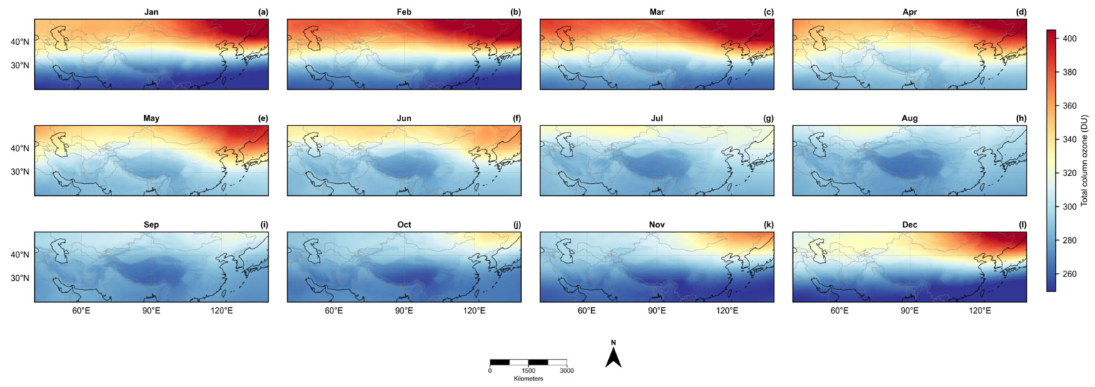
Figure A2.
Seasonal distributions of total column ozone and zonal anomalies over the Tibetan Plateau and surrounding mid-latitude region (20–50°N, 40–140°E). (a–d) Total column ozone (TCO) in spring (MAM), summer (JJA), autumn (SON), and winter (DJF); (e–h) corresponding zonal anomalies.
References
- Zhou, X.; Luo, C. Ozone valley over Tibetan Plateau. Acta Meteorol. Sin. 1994, 8, 505–506. (In Chinese) [Google Scholar]
- Zhou, X.; Luo, C.; Li, W.; Shi, J. Total ozone changes in China and the low center over the Tibetan Plateau. Chin. Sci. Bull. 1995, 40, 1396–1398. (In Chinese) [Google Scholar]
- Zhou, X.; Li, W.; Chen, L.; Liu, Y. Study of the atmospheric ozone variation over the Tibetan Plateau. Acta Meteorol. Sin. 2004, 62, 513–527. (In Chinese) [Google Scholar]
- Zou, H. Seasonal variation and trends of TOMS ozone over Tibet. Geophys. Res. Lett. 1996, 23, 1029–1032. [Google Scholar] [CrossRef] [Scilit]
- Forster, P.M.F.; Shine, K.P. Stratospheric water vapour changes as a possible contributor to observed stratospheric cooling. Geophys. Res. Lett. 1999, 26, 3309–3312. [Google Scholar] [CrossRef] [Scilit]
- Xia, Y.; Huang, Y.; Hu, Y. On the climate impacts of upper tropospheric and lower stratospheric ozone. J. Geophys. Res. Atmos. 2017, 123, 730–739. [Google Scholar] [CrossRef] [Scilit]
- Guo, D.; Su, Y.; Shi, C.; Xu, J.; Powell, A.M. Double core of ozone valley over the Tibetan Plateau and its possible mechanisms. J. Atmos. Sol.-Terr. Phys. 2015, 130–131, 127–131. [Google Scholar] [CrossRef] [Scilit]
- Guo, D.; Xu, J.; Su, Y.; Shi, C.; Sun, J. Comparison of the vertical structure and formation mechanism of the summer ozone valley over the Tibetan Plateau and North America. Trans. Atmos. Sci. 2017, 40, 412–417. (In Chinese) [Google Scholar] [CrossRef]
- Ma, X.; Xu, J.; Lin, C.; Shi, J. Spatio-temporal characteristics analysis of ozone valley on the Qinghai-Xizang Plateau based on satellite data. Chin. J. Space Sci. 2025, 45, 1272–1284. (In Chinese) [Google Scholar] [CrossRef] [Scilit]
- Randel, W.J.; Park, M. Deep convective influence on the Asian summer monsoon anticyclone and associated tracer variability observed with Atmospheric Infrared Sounder (AIRS). J. Geophys. Res. Atmos. 2006, 111, D12314. [Google Scholar] [CrossRef] [Scilit]
- Tian, W.; Chipperfield, M.P.; Huang, Q. Effects of the Tibetan Plateau on total column ozone distribution. Tellus B 2008, 60, 622–635. [Google Scholar] [CrossRef] [Scilit]
- Bian, J.; Yan, R.; Chen, H.; Lü, D.; Massie, S.T. Formation of the summertime ozone valley over the Tibetan Plateau: The Asian summer monsoon and air column variations. Adv. Atmos. Sci. 2011, 28, 1318–1325. [Google Scholar] [CrossRef] [Scilit]
- Basha, G.; Ratnam, M.V.; Kishore, P. Asian summer monsoon anticyclone: Trends and variability. Atmos. Chem. Phys. 2020, 20, 6789–6801. [Google Scholar] [CrossRef] [Scilit]
- Keppens, A.; Di Pede, S.; Hubert, D.; Lambert, J.-C.; Veefkind, P.; Sneep, M.; De Haan, J.; ter Linden, M.; Leblanc, T.; Compernolle, S.; et al. 5 years of Sentinel-5P TROPOMI operational ozone profiling and geophysical validation using ozonesonde and lidar ground-based networks. Atmos. Meas. Tech. 2024, 17, 3969–3993. [Google Scholar] [CrossRef] [Scilit]
- Bak, J.; Liu, X.; González Abad, G.; Yang, K. An Extension of Ozone Profile Retrievals from TROPOMI Based on the SAO2024 Algorithm. Remote Sens. 2025, 17, 779. [Google Scholar] [CrossRef] [Scilit]
- Freitas, A.D.; Zacharias, D.C.; Paim, B.L.; Borbon, A.; Fornaro, A. Investigating Ozone Formation Regimes in the Metropolitan Area of São Paulo Using Five Years of TROPOMI HCHO/NO2 Ratios. Remote Sens. 2026, 18, 1603. [Google Scholar] [CrossRef] [Scilit]
- Li, Z. Extracting spatial effects from machine learning model using local interpretation method: An example of SHAP and XGBoost. Comput. Environ. Urban Syst. 2022, 96, 101845. [Google Scholar] [CrossRef] [Scilit]
- Van den Broeck, G.; Lykov, A.; Schleich, M.; Suciu, D. On the tractability of SHAP explanations. J. Artif. Intell. Res. 2022, 74, 851–886. [Google Scholar] [CrossRef] [Scilit]
- Tang, Y.; Duan, A.; Xiao, C.; Xin, Y. The Prediction of the Tibetan Plateau Thermal Condition with Machine Learning and Shapley Additive Explanation. Remote Sens. 2022, 14, 4169. [Google Scholar] [CrossRef] [Scilit]
- Xu, J.; Zhang, Z.; Rao, L.; Wang, Y.; Letu, H.; Shi, C.; Tana, G.; Wang, W.; Zhu, S.; Liu, S.; et al. Remote sensing of tropospheric ozone from space: Progress and challenges. J. Remote Sens. 2024, 4, 0178. [Google Scholar] [CrossRef] [Scilit]
- Xu, J.; Zhang, Z.; Rao, L.; Wang, Y.; Yan, H.; Husi, L.; Shi, C.; Liu, S.; Gegen, T.; Wang, W.; et al. Tropospheric ozone retrieval from satellite remote sensing—A review. Adv. Earth Sci. 2024, 39, 56–70. Available online: https://www.geores.com.cn/dqkxjz/EN/10.11867/j.issn.1001-8166.2024.002 (accessed on 30 May 2026).
- Shi, C.; Zhang, C.; Guo, D. Comparison of Electrochemical Concentration Cell Ozonesonde and Microwave Limb Sounder Satellite Remote Sensing Ozone Profiles for the Center of the South Asian High. Remote Sens. 2017, 9, 1012. [Google Scholar] [CrossRef] [Scilit]
- Hersbach, H.; Bell, B.; Berrisford, P.; Hirahara, S.; Horányi, A.; Muñoz-Sabater, J.; Nicolas, J.; Peubey, C.; Radu, R.; Schepers, D.; et al. The ERA5 global reanalysis. Q. J. R. Meteorol. Soc. 2020, 146, 1999–2049. [Google Scholar] [CrossRef] [Scilit]
- Farr, T.G.; Rosen, P.A.; Caro, E.; Crippen, R.; Duren, R.; Hensley, S.; Kobrick, M.; Paller, M.; Rodriguez, E.; Roth, L.; et al. The Shuttle Radar Topography Mission. Rev. Geophys. 2007, 45, RG2004. [Google Scholar] [CrossRef] [Scilit]
- Wei, W.; Zhang, R.; Wen, M.; Kim, B.-J.; Nam, J.-C. Interannual variation of the South Asian High and its relation with Indian and East Asian summer monsoon rainfall. J. Clim. 2015, 28, 2623–2634. [Google Scholar] [CrossRef] [Scilit]
- Holton, J.R.; Haynes, P.H.; McIntyre, M.E.; Douglass, A.R.; Rood, R.B.; Pfister, L. Stratosphere-troposphere exchange. Rev. Geophys. 1995, 33, 403–439. [Google Scholar] [CrossRef] [Scilit]
- World Meteorological Organization. Meteorology—A three-dimensional science: Second session of the Commission for Aerology. WMO Bull. 1957, 6, 134–138. [Google Scholar]
- Efron, B.; Tibshirani, R.J. An Introduction to the Bootstrap; Chapman and Hall/CRC: New York, NY, USA, 1994. [Google Scholar] [CrossRef] [Scilit]
- Granger, C.W.J. Investigating causal relations by econometric models and cross-spectral methods. Econometrica 1969, 37, 424–438. [Google Scholar] [CrossRef] [Scilit]
- Chen, T.; Guestrin, C. XGBoost: A scalable tree boosting system. In Proceedings of the 22nd ACM SIGKDD International Conference on Knowledge Discovery and Data Mining, San Francisco, CA, USA, 13–17 August 2016; ACM: New York, NY, USA, 2016; pp. 785–794. [Google Scholar] [CrossRef] [Scilit]
- Lundberg, S.M.; Lee, S.-I. A unified approach to interpreting model predictions. In Advances in Neural Information Processing Systems 30; Curran Associates: Red Hook, NY, USA, 2017; pp. 4765–4774. [Google Scholar]
- Xu, W.; Guo, D.; Sun, X.; Shi, C.; Chen, D.; Duan, M.; Rao, J.; Du, Y.; Tang, Z. Definition and characteristics of extreme events of ozone valley over the Tibetan Plateau. Trans. Atmos. Sci. 2019, 42, 129–137. (In Chinese) [Google Scholar] [CrossRef]
- Qiu, Y.; Wei, M.; Jiang, A.; Tong, J. General characteristics of the ozone low center above the Tibetan Plateau and (low) trough above the Rocky Mountains—On the cause of static deficit/depletion above the high mountains. Clim. Environ. Res. 2008, 13, 617–628. (In Chinese) [Google Scholar]
- Qin, H.; Guo, D.; Shi, C.; Li, Z.; Zhou, S.; Huang, Y.; Su, Y.; Wang, L. The interaction between variations of the South Asian High and ozone in the adjacent regions. Chin. J. Atmos. Sci. 2018, 42, 421–434. (In Chinese) [Google Scholar] [CrossRef]
- Guo, D.; Wang, P.; Zhou, X.; Liu, Y.; Li, W. Dynamic effects of the South Asian High on the ozone valley over the Tibetan Plateau. Acta Meteorol. Sin. 2012, 26, 216–228. [Google Scholar] [CrossRef] [Scilit]
- Legras, B.; Bucci, S. Confinement of air in the Asian monsoon anticyclone and pathways of convective air to the stratosphere during the summer season. Atmos. Chem. Phys. 2020, 20, 11045–11064. [Google Scholar] [CrossRef] [Scilit]
- Yang, Q.; Zhao, T.; Bai, Y.; Meng, K.; Luo, Y.; Tian, Z.; Sun, X.; Fu, W.; Yang, K.; Hu, J. Distinct structures of interannual variations in stratosphere-to-troposphere ozone transport induced by the Tibetan Plateau thermal forcing. Atmos. Chem. Phys. 2025, 25, 8029–8042. [Google Scholar] [CrossRef] [Scilit]
- Zhang, Z.; Chen, Q.; Yuan, C. Spatial and temporal variation characteristics of the tropopause over the Tibetan Plateau. Arid Zone Res. 2016, 33, 690–697. (In Chinese) [Google Scholar] [CrossRef]
- Chen, P.; Li, Y.; Jing, G.; Chang, S. Analysis of the formation mechanism of the stratospheric ozone valley over the Qinghai-Xizang Plateau. Plateau Meteorol. 2023, 42, 1182–1193. (In Chinese) [Google Scholar] [CrossRef]
- Škerlak, B.; Sprenger, M.; Wernli, H. A global climatology of stratosphere-troposphere exchange using the ERA-Interim data set from 1979 to 2011. Atmos. Chem. Phys. 2014, 14, 913–937. [Google Scholar] [CrossRef] [Scilit]
- Li, T.; Wu, N.; Chen, J.; Chan, P.-W.; Tang, J.; Wang, N. Vertical exchange and cross-regional transport of lower-tropospheric ozone over Hong Kong. Atmos. Res. 2023, 292, 106877. [Google Scholar] [CrossRef] [Scilit]
- Li, Y.; Xia, Y.; Xie, F.; Yan, Y. Influence of stratosphere-troposphere exchange on long-term trends of surface ozone in CMIP6. Atmos. Res. 2024, 297, 107086. [Google Scholar] [CrossRef] [Scilit]
- Trisolino, P.; Putero, D.; Arduini, J.; Amendola, S.; Calzolari, F.; Cristofanelli, P. Influence of deep stratosphere-to-troposphere transport on atmospheric carbon dioxide and methane at the Mt. Cimone WMO/GAW global station (2165 m a.s.l., Italy): A multi-year (2015–2022) investigation. Atmos. Res. 2024, 310, 107627. [Google Scholar] [CrossRef] [Scilit]
- Shu, Z.; Yang, F.; Shi, G.; Zhang, Y.; Huang, Y.; Yu, X.; Pan, B.; Zhao, T. Impact of stratospheric intrusion on near-surface ozone over the Sichuan Basin in China driven by terrain forcing of Tibetan Plateau. Atmos. Chem. Phys. 2025, 25, 15437–15451. [Google Scholar] [CrossRef] [Scilit]
- Chang, S.; He, H.; Huang, D. The effects of gravity waves on ozone over the Tibetan Plateau. Atmos. Res. 2024, 299, 107204. [Google Scholar] [CrossRef] [Scilit]
- Guo, K.; Huang, Q.; Dai, Y.; Zhang, Y.; Wang, Z.; Du, J.; Chou, Y. Clear air turbulence over the Tibetan Plateau and its effect on ozone transport in the upper troposphere-lower stratosphere. Atmos. Res. 2025, 318, 108005. [Google Scholar] [CrossRef] [Scilit]
- Zhang, D.; Huang, Y.; Zhou, B.; Wang, H. Is there interdecadal variation in the South Asian High? J. Clim. 2021, 34, 8089–8103. [Google Scholar] [CrossRef] [Scilit]
- Cen, S.; Chen, W.; Chen, S.; Wang, L.; Liu, Y.; Huangfu, J. Weakened influence of El Niño–Southern Oscillation on the zonal shift of the South Asian High after the early 1980s. Int. J. Climatol. 2022, 42, 7583–7597. [Google Scholar] [CrossRef] [Scilit]
- Roy, C.; Fadnavis, S.; Sabin, T.P. The stratospheric ozone rich cold intrusion during El-Niño over the Indian region: Implication during the Indian summer monsoon. Int. J. Climatol. 2021, 41, E233–E248. [Google Scholar] [CrossRef] [Scilit]
- Wang, Y.; Zhao, P.; Xu, H.; Liu, G. Anomalies of Northern Hemisphere ozone associated with a tropopause-lower stratosphere teleconnection during summer. Int. J. Climatol. 2015, 36, 837–846. [Google Scholar] [CrossRef] [Scilit]
- Chang, S.; Li, Y.; Shi, C.; Guo, D. Combined Effects of the ENSO and the QBO on the Ozone Valley over the Tibetan Plateau. Remote Sens. 2022, 14, 4935. [Google Scholar] [CrossRef] [Scilit]
- Li, Y.; Xu, F.; Wan, L.; Chen, P.; Guo, D.; Chang, S.; Yang, C. Effect of ENSO on the Ozone Valley over the Tibetan Plateau Based on the WACCM4 Model. Remote Sens. 2023, 15, 525. [Google Scholar] [CrossRef] [Scilit]
- Wang, W.; Liu, X.; Bi, J.; Liu, Y. A machine learning model to estimate ground-level ozone concentrations in California using TROPOMI data and high-resolution meteorology. Environ. Int. 2022, 158, 106917. [Google Scholar] [CrossRef] [Scilit] [PubMed]
- Luo, Z.; Lu, P.; Chen, Z.; Liu, R. Ozone concentration estimation and meteorological impact quantification in the Beijing-Tianjin-Hebei region based on machine learning models. Earth Space Sci. 2024, 11, e2023EA003346. [Google Scholar] [CrossRef] [Scilit]
- Jiang, Q.; Wang, N.; Jin, Z.; Sun, X.; Wang, J.; Li, R. Combining machine learning to explore the influence of VOCs and meteorological factors on ozone concentration: A case study of a chemical park in Shenyang, China. Atmos. Res. 2025, 322, 108113. [Google Scholar] [CrossRef] [Scilit]
- Xiao, Z.; Jiang, C.; Hao, S.; Chan, K.L. Insights into regional tropospheric ozone trends and driving factors in China (2015–2020) using WRF-Chem and global sensitivity analysis. J. Geophys. Res. Atmos. 2025, 130, e2025JD044687. [Google Scholar] [CrossRef] [Scilit]
- Li, K.; Tan, R.; Qiao, W.; Lee, T.; Wang, Y.; Zhang, D.; Tang, M.; Zhao, W.; Gu, Y.; Fan, S.; et al. Surface and tropospheric ozone over East Asia and Southeast Asia from observations: Distributions, trends, and variability. Atmos. Chem. Phys. 2025, 25, 11575–11596. [Google Scholar] [CrossRef] [Scilit]
- Wang, C.; Liu, Y.; Wang, W.; Deng, L.; Sun, X.; Liu, G.; Shao, H.; Jin, Z. What makes the lower urban land coverage city a deeper ozone trap: Implications from a case study in the Sichuan Basin, Southwest China. Remote Sens. 2026, 18, 1657. [Google Scholar] [CrossRef] [Scilit]
- Lu, G.; Li, Q.; Sun, X.; Zhao, M.; Dong, L.; Wu, Q.; Wang, L.; Zhao, L.; Duan, C.; Yin, Y.; et al. Comparative analysis of peak-summer heatwaves in the Yangtze–Huaihe River Basin of China in 2022 and 2013: Thermal effects of the Tibetan Plateau. Atmos. Res. 2024, 300, 107222. [Google Scholar] [CrossRef] [Scilit]
- Jin, Z.; Xu, K.; Ge, F.; Wang, W.; Lin, Z. Boost to early spring compound heatwaves over South Asia from anomalous Tibetan Plateau atmospheric heat source. Atmos. Res. 2024, 305, 107449. [Google Scholar] [CrossRef] [Scilit]
- Adeniran, I.A.; Nazeer, M.; Wong, M.S.; Yang, J.; Chan, P.-W. Diurnal air–surface temperature dynamics in Hong Kong: An analysis across land use and climate zones. Int. J. Climatol. 2026, 46, e70297. [Google Scholar] [CrossRef] [Scilit]
- Hong, S.; Bak, J.; Keppens, A.; Yang, K.; Baek, K.; Liu, X.; Kim, M.; Kim, J.; Chang, L.-S.; Lee, H.; et al. Cross-Validation of GEMS Total Ozone from Ozone Profile and Total Column Products Using Pandora and Satellite Observations. Remote Sens. 2025, 17, 3249. [Google Scholar] [CrossRef] [Scilit]
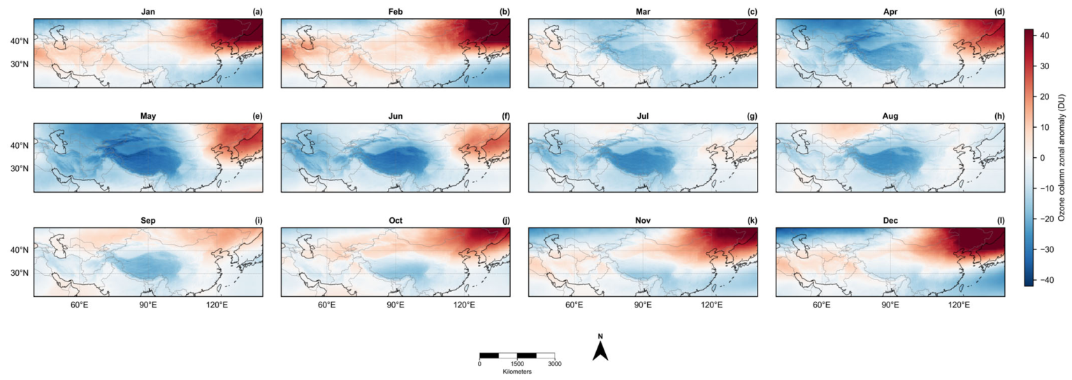
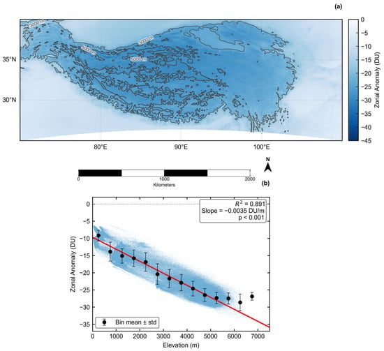
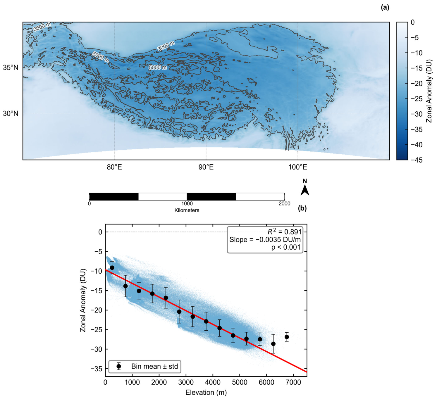
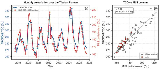
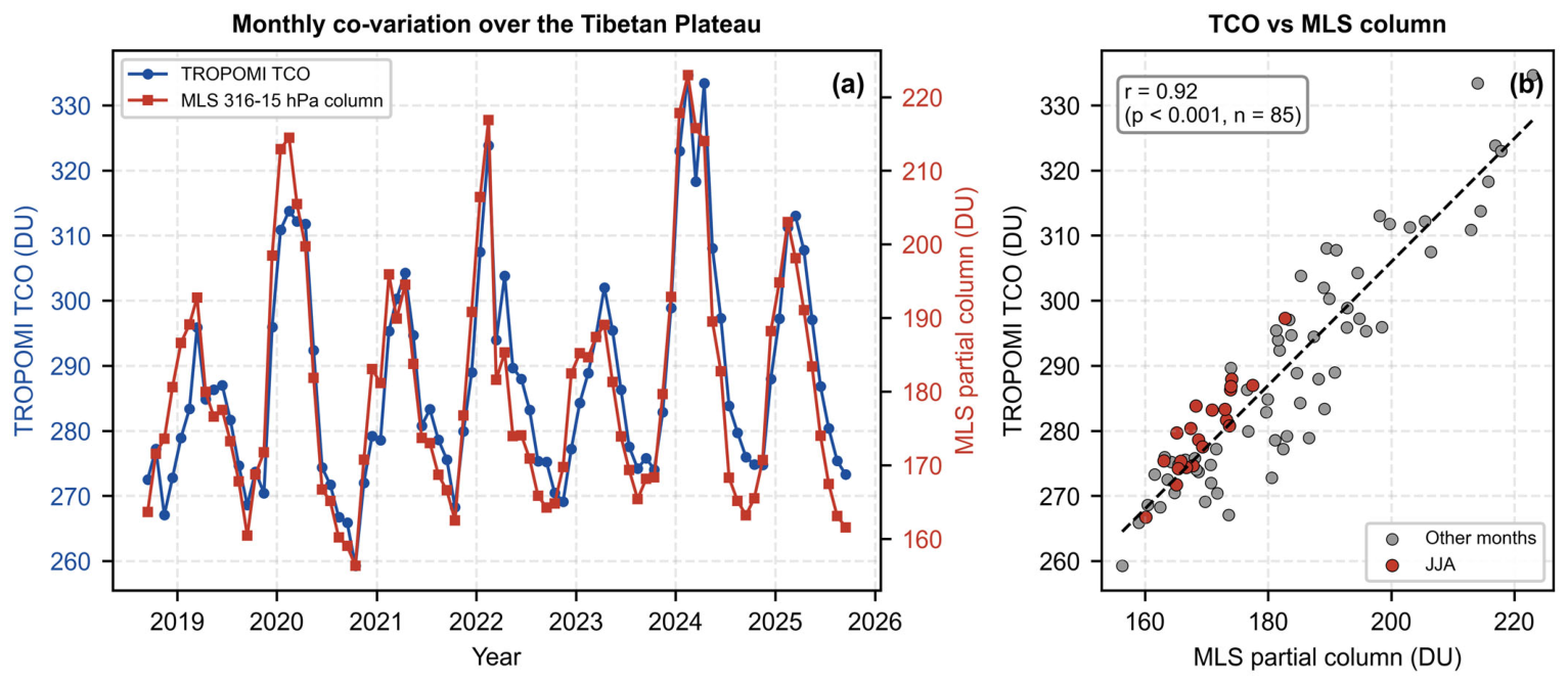
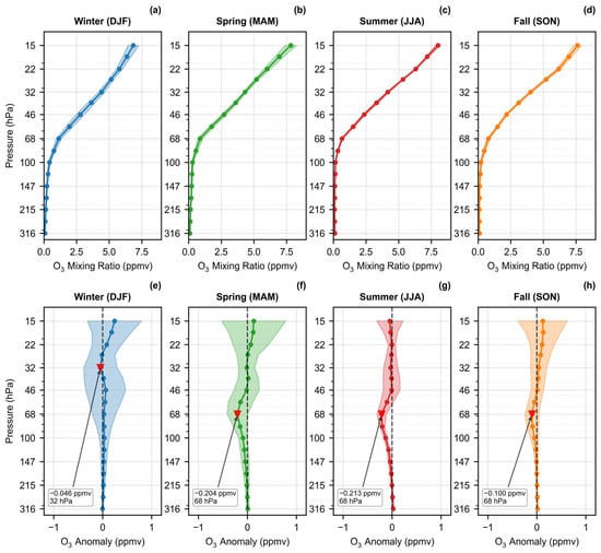
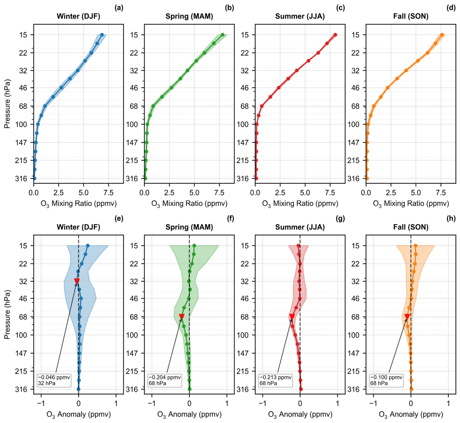
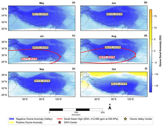
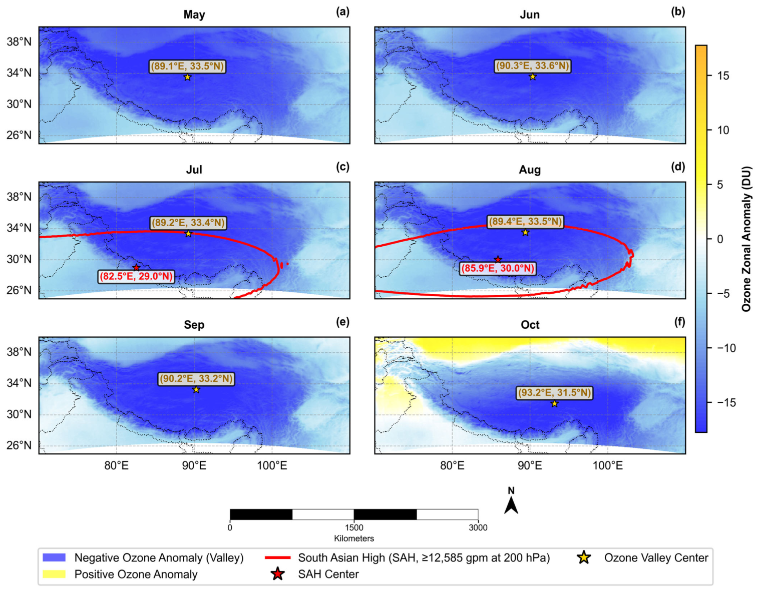
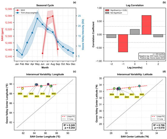
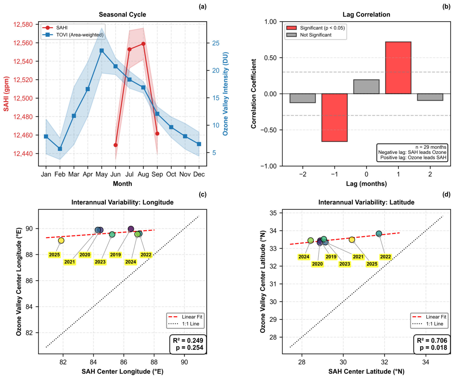
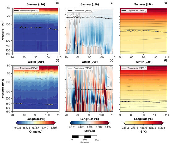
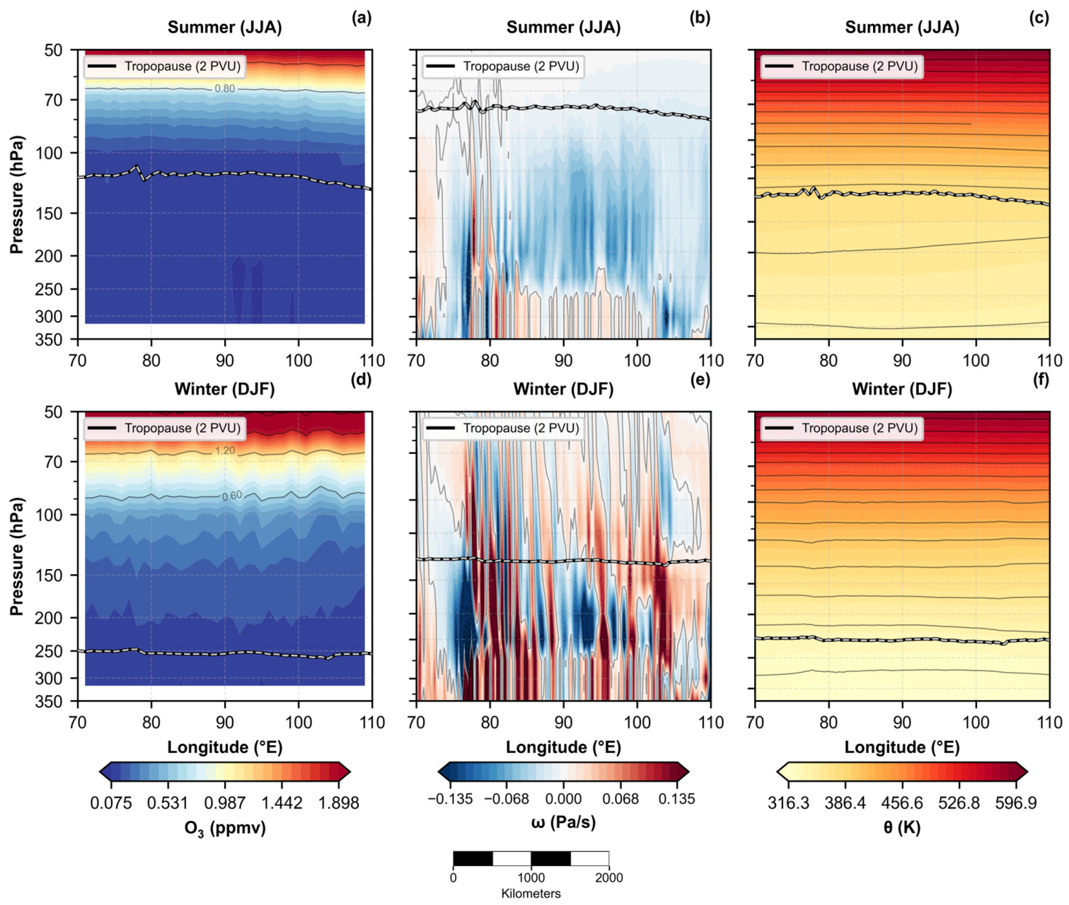
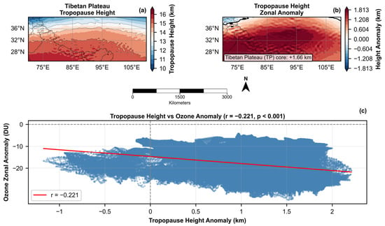
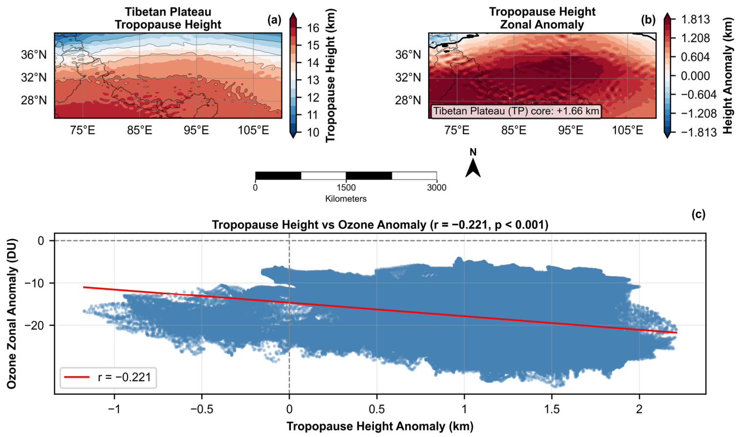
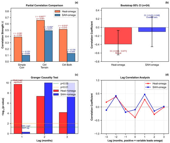
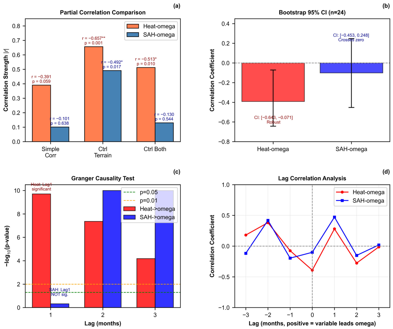
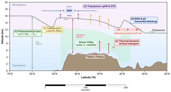
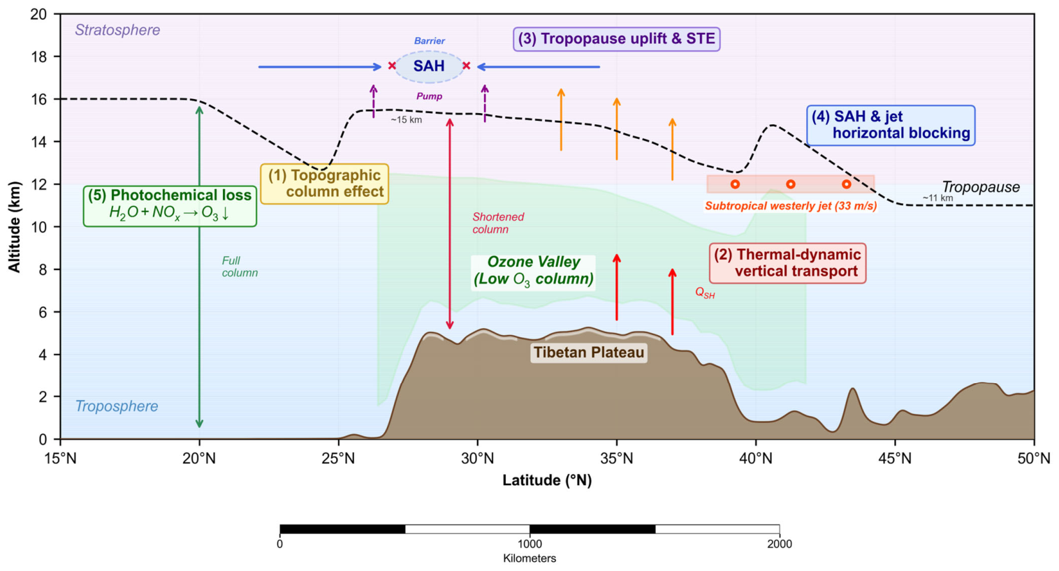

Disclaimer/Publisher’s Note: The statements, opinions and data contained in all publications are solely those of the individual author(s) and contributor(s) and not of MDPI and/or the editor(s). MDPI and/or the editor(s) disclaim responsibility for any injury to people or property resulting from any ideas, methods, instructions or products referred to in the content. |
© 2026 by the authors. Licensee MDPI, Basel, Switzerland. This article is an open access article distributed under the terms and conditions of the Creative Commons Attribution (CC BY) license.