


Highlights
What are the main findings?
- Satellite-derived vegetation indices revealed substantial declines in urban grassland greenness during prolonged drought, with the most pronounced deficits occurring in summer; time-series decomposition and anomaly analyses further demonstrated that these impacts persisted over multiple years, indicating sustained ecological stress rather than short-term climatic fluctuations.
- Temperature exerted a stronger and more consistent influence on vegetation condition than rainfall, while the focus on grass-dominated urban green spaces enhanced the detection of climate sensitivity; collectively, these findings support the concept of “urban greenery drought,” whereby heat stress drives vegetation decline despite the presence of irrigation and rainfall inputs.
What are the implications of the main findings?
- Urban green space management may benefit from considering temperature alongside water availability, as temperature was found to be a stronger driver of NDVI variability than rainfall. Measures such as the use of heat-tolerant and drought-resistant species, adaptive irrigation scheduling, and urban design approaches that reduce heat exposure may contribute to maintaining vegetation condition during periods of combined heat and drought stress.
- The greater drought sensitivity of shallow-rooted lawn vegetation and the observed incomplete post-drought recovery highlight differences in vegetation responses within urban green spaces. These findings suggest that management approaches tailored to vegetation characteristics, together with water-sensitive urban design, alternative water sources, and long-term green infrastructure planning, may support vegetation function and urban cooling under projected increases in drought frequency and climatic aridity.
Abstract
Urban green spaces (UGSs) are vital for enhancing a city’s resilience and livability; however, their functionality is increasingly jeopardized by drought, particularly in water-scarce regions. This study evaluates drought impact on UGSs in Metropolitan Adelaide, Australia, a representative semi-arid urban system, using satellite-derived Normalized Difference Vegetation Index (NDVI) time-series data spanning 2000–2020. Vegetation dynamics were analyzed through Seasonal-Trend decomposition using Loess (STL), standardized anomaly assessment, lagged Pearson correlation, Ordinary Least Squares (OLS) regression, and Mann–Kendall trend analysis. To isolate climatically sensitive signals, 29 urban lawn patches were examined separately from mixed urban canopy, given their shallow root systems and direct dependence on surface moisture. NDVI declined by approximately 0.09 units during the Millennium Drought (2001–2009), with summer greenness deficits reaching 24% below the 20-year benchmark. Temperature was the dominant driver of lawn NDVI variability (r = −0.863, R2 = 74.5%), substantially exceeding the effect of rainfall (r = 0.156, R2 = 2.4%). El Niño–Southern Oscillation (ENSO) cycles modulated vegetation responses, with La Niña years supporting recovery and El Niño years amplifying decline. Post-drought recovery remained incomplete, with NDVI deficits of 8–20% persisting through 2020; full recovery was observed only in 2017, coinciding with the highest recorded summer rainfall. No significant directional trend was detected over the full study period (Mann–Kendall τ = 0.005, p = 0.908). These findings demonstrate that heat, rather than water limitation alone, is the primary driver of vegetation stress in urban systems, highlighting the benefits of integrated management strategies that address both warming and moisture deficits to sustain urban green infrastructure under future climate conditions. We introduce the concept of “urban greenery drought,” referring to a form of vegetation stress in managed urban landscapes where greenness is reduced primarily by elevated temperature and atmospheric demand despite water availability.
1. Introduction
Green spaces contribute to the regulation of microclimates by providing shade, which mitigates surface heating, and enhancing actual evapotranspiration (AET), a process that contributes to cooling the surrounding atmosphere [1,2,3,4,5,6,7]. Green spaces encompass areas covered by vegetation, including forests, grasslands, wetlands, and agricultural lands. Within urban contexts, these spaces are referred to as UGSs, which include public parks, gardens, tree-lined streets, and urban forests. These UGSs serve as buffers against extreme climate events [8,9]. These spaces support urban livability through ecosystem services such as heat wave mitigation, air and water purification, carbon sequestration, biodiversity conservation, and climate regulation [10]. They contribute to psychological and physiological well-being. Among the various components of urban green spaces (UGSs), lawns support ecological, environmental, and social functions. Globally, lawns are the most common elements of urban green spaces, covering up to 50–70% of urban green areas regardless of climatic conditions or water availability [11]. In Australian cities specifically, the total area under turf is approximately 4400 hectares, constituting an average of 11% of the total area of cities [11]. Lawn plays a unique role in regulating the urban microclimate by reducing surface wind speeds and maintaining higher albedo compared to dark impervious surfaces [12]. Observational data from 54 heatwave events in a subtropical city over ten years showed that lawns, with high canopy stomatal conductance, rapidly increased evapotranspiration by 37.65% during heatwaves and provided substantial cooling of 7.05 °C m−2 per day. By contrast, trees provided a lower cooling effect of 3.5 °C m−2 per day. This divergence in water-use strategy is precisely what motivates using lawn patches, rather than treed areas, to detect surface-level climate signals [13].
Urban green spaces (UGSs) contribute to mitigating Urban Heat Island (UHI) effects, a phenomenon where urban areas experience higher temperatures than surrounding rural regions due to factors including impervious surfaces and reduced vegetation [14]. Although UGSs contribute to many ecosystem services, their capacity to reduce UHI effects is associated with public health and comfort outcomes during extreme heat events [8]. This function is especially relevant in densely populated cities, where built surfaces amplify heat retention and exacerbate the frequency and intensity of heat waves [10,15]. However, the functionality and sustainability of spaces are increasingly threatened by climate change-induced stressors, particularly drought, which exacerbates water scarcity and vegetation stress [16,17,18]. Despite growing concern about climate-induced drought in Australian cities, the long-term response of urban green spaces to prolonged dry conditions remains insufficiently quantified, particularly in Mediterranean-type climates such as Metropolitan Adelaide [19,20]. Also, the quantitative assessment of drought-induced vegetation stress in urban green spaces remains insufficiently addressed in the Australian context. Consequently, urban planners and climate adaptation practitioners in Adelaide lack a spatially explicit, evidence-based quantitative baseline for evaluating the drought resilience of existing UGSs. This study addresses that gap by employing Normalized Difference Vegetation Index (NDVI)-derived remote sensing analysis to provide a replicable, quantitative assessment of drought impact on UGSs across Adelaide, thereby supporting the development of climate-adaptive urban greening strategies grounded in empirical evidence. Urban environments present unique conditions, including fragmented vegetation patches, heterogeneous land cover, and intensive human management practices, which can influence vegetation resilience to water stress.
Remote sensing techniques, particularly vegetation indices derived from satellite imagery, can be used to monitor vegetation dynamics over large spatial and temporal scales. Remote sensing indicators, particularly NDVI, are used to evaluate vegetation dynamics over time; however, their use in assessing drought impact on urban ecosystems over multi-decadal scales is limited.
Since the early 2000s, Metropolitan Adelaide has faced increasing pressure on its urban green spaces (UGSs) due to population growth, urban intensification, and land-use change. Current assessments indicate that tree canopy covers approximately 17% of metropolitan Adelaide, below the 30% canopy target associated with improved urban resilience and livability [21,22]. Despite greening initiatives, Adelaide’s urban forest remains vulnerable, with 69% of trees below 10 m in height, limiting long-term canopy benefits [21,22]. Urban heat intensity also increased by approximately 0.2 °C between 2014 and 2023, highlighting the potential role of additional greening interventions in mitigating urban heat [21,22]. The Urban Greening Strategy (2025) aims to increase canopy cover from 17% to 30% by 2055, supporting cooler, greener, and more biodiverse urban environments. This strategy aligns with the Greater Adelaide Regional Plan, which addresses projected population growth of 670,000 people and 315,000 new homes by 2050 while incorporating additional green and open spaces [23].
Drought may disrupt the equilibrium of urban green spaces (UGSs) by limiting the water resources required for sustaining vegetation health [24,25]. Multiple studies confirm that NDVI declines substantially during periods of drought or when irrigation is restricted [26,27,28,29]. For example, research in Adelaide found that parklands dependent on irrigation exhibited lower NDVI values during summer droughts when blue water resources were scarce; city councils allowed grasslands to dry out seasonally due to water shortages [27,30].
We investigate the effects of prolonged dry periods on UGSs’ functionality, focusing on how drought conditions degrade vegetation greenness, as quantified by declining NDVI values (a proxy for vegetation greenness, referring to Chavoshi Borujeni et al. [31,32,33]). Drought is a recurrent feature of South Australia’s climate. Yet, previous research has focused less on UGSs, as water availability has more commonly been quantified in agricultural ecosystems in relation to food production and security. While Pataki et al. [34] highlighted the water stress as a global challenge to urban tree health, species-specific adaptive mechanisms within the unique climatic and ecological conditions of Metropolitan Adelaide remain underexplored. This gap underscores the value of a comprehensive investigation into localized arboreal resilience, particularly as urbanization intensifies pressure on water resources in semi-arid regions. To address this gap, this study investigates how drought conditions affect vegetation conditions within UGSs across Metropolitan Adelaide by quantifying spatiotemporal changes in NDVI across drought and non-drought periods. The findings are subsequently used to identify spatially differentiated patterns of drought vulnerability, thereby providing an empirical basis for informing climate-adaptive UGS management strategies. In semi-arid regions like Adelaide, rapid urbanization increases impervious surfaces, alters local microclimates, and strains water resources, influencing urban green space (UGS) management. We discuss the challenges of sustaining UGSs during drought events, advancing resilience discourse, and proposing a potential sustainable management strategy that can be applicable to Metropolitan Adelaide and similar urban settings.
This study aims to comprehensively assess the multifaceted impact of drought on UGSs in Metropolitan Adelaide, a region increasingly challenged by climate-driven aridity. Specifically, it combines satellite-derived NDVI, climate data, and statistical analysis to characterize drought-induced vegetation. We quantify drought-associated changes in NDVI across urban green spaces in Metropolitan Adelaide over the 2000–2020 period and identify patterns of vegetation decline and recovery that can inform evidence-based adaptive management decisions.
There are five specific objectives of this study.
- The first objective is to quantify drought-induced vegetation decline in Metropolitan Adelaide’s urban green spaces. The study sets out to measure the magnitude of NDVI reduction during the Millennium Drought (2001–2009) and post-drought period (2010–2020), establishing a 20-year benchmark against which seasonal and interannual greenness deficits are assessed.
- The next objective is to identify the primary climatic drivers of urban vegetation variability. The paper tests whether rainfall or temperature exerts a stronger influence on NDVI, using both parametric (Pearson, OLS) and non-parametric (Spearman, Mann–Whitney) methods to ensure robustness across the non-normally distributed dataset.
- Another objective is to assess seasonal aridity patterns and their hydroclimatic context. The study characterizes Adelaide’s dry-month structure and examines how ENSO variability (La Niña and El Niño cycles) modulates interannual fluctuations in vegetation greenness beyond the climatological baseline.
- Following this, an objective is to evaluate post-drought vegetation recovery and ecological memory. The paper explicitly investigates whether NDVI returned to pre-drought levels following the Millennium Drought, and whether the rate and completeness of recovery can be attributed to rainfall alone or are constrained by cumulative drought legacies.
- The last objective is to translate remote sensing findings into potential urban planning recommendations. The study aims to connect satellite-derived vegetation indicators to potential actionable management strategies, including drought-tolerant species selection, smart irrigation, and heat-responsive planning for water-scarce cities.
Quantitative remote sensing studies that isolate the direct effects of drought and thermal stress on urban vegetation, independent of irrigation-buffered canopy responses, remain limited in the literature. Studies that apply aggregated NDVI across heterogeneous urban cover frequently mask drought signals, as deep-rooted trees maintain access to groundwater independently of surface precipitation. The relative contributions of rainfall and temperature to vegetation conditions are also rarely disentangled at sub-seasonal resolution in managed urban settings. This study addresses these gaps by analyzing satellite-derived NDVI time-series data (2000–2020) for Metropolitan Adelaide, Australia, a semi-arid Mediterranean-climate city representative of water-scarce urban environments globally.
The specific contributions of this study are as follows:
- A methodological approach that separates 29 urban lawn patches from mixed-canopy cover to isolate climatically sensitive NDVI signals, directly addressing the masking effect of deep-rooted vegetation that attenuates drought responses in aggregate urban vegetation analyses.
- Quantitative evidence that temperature is the dominant climatic driver of urban lawn greenness (R2 = 74.5%), substantially outweighing the effect of rainfall (R2 = 2.4%), which challenges water-centric assumptions that underpin much of current UGS management practice.
- Documentation of ecological memory effects in a managed urban setting, demonstrating that post-Millennium Drought NDVI deficits of 8–20% persisted through 2020, with full seasonal recovery achieved only under exceptional rainfall conditions in 2017.
- Empirical evidence that active irrigation maintained baseline NDVI during the drought period without preventing cumulative greenness deterioration, distinguishing between buffered baseline performance and suppressed peak vegetation condition.
- An integrated multi-method analytical framework combining STL decomposition, lagged Pearson and Spearman correlation, OLS regression, Mann–Kendall trend analysis, and Wilcoxon phase comparison, characterizing urban vegetation–climate dynamics at sub-seasonal resolution across two contrasting hydroclimatic periods.
2. Materials and Methods
2.1. Study Area
Metropolitan Adelaide contains the city, the capital of South Australia, and spans latitudes 34.7–35.1°S and longitudes 138.4–138.8°E on the eastern shores of the Gulf St Vincent [35] (Figure 1). Covering approximately 3260 km2, it is Australia’s fifth-largest urban center, with a population of 1.4 million as of 2021 [36]. Adelaide’s population grew at an annual rate of 0.8% between 2016 and 2021, with projections indicating growth to 1.7 million by 2041, which increases pressure on UGSs [36,37]. This growth intensifies land-use competition, leading to potential encroachment on green spaces and heightened demand for their ecosystem services. Metropolitan Adelaide experiences a Mediterranean climate (Köppen Csa), characterized by hot, dry summers and cool, wet winters. Long-term climate records indicate a mean maximum summer temperature of approximately 28.8 °C (peaking at 29.6 °C in January), a mean minimum winter temperature of approximately 8 °C, and a mean annual rainfall of approximately 541 mm, concentrated predominantly in the winter months from June to August, when monthly totals average 68–78 mm [38]. Urban green spaces (UGSs), including the Adelaide Park Lands, are unevenly distributed across Metropolitan Adelaide. A study of Australia’s five largest capital cities found that Adelaide exhibited the least equitable distribution of green space, with approximately 20% green cover in the most affluent neighborhoods compared with 12% in the least affluent areas [39]. This pattern indicates broader concerns regarding environmental equity, as socioeconomically disadvantaged communities often experience lower access to green infrastructure and its associated health and environmental benefits. Unequal access to UGSs may exacerbate exposure to urban heat and reduce opportunities for recreation, biodiversity conservation, and wellbeing [40]. Metropolitan Adelaide’s water supply is sourced from River Murray transfers, surface-water storage, groundwater, and desalination. According to the Bureau of Meteorology’s National Water Account for 2021–2022, water sourced in the Adelaide region comprised approximately 44% inter-region deliveries from the River Murray, 34% surface water, 19% groundwater, and 2% desalinated water. The Adelaide Desalination Plant has a design capacity of approximately 100 GL per year, almost half of Adelaide’s annual water demand, but typically operates at much lower output. Supply proportions vary considerably between years depending on rainfall, reservoir inflows, and River Murray transfers, highlighting the influence of climate variability on Adelaide’s water security. Groundwater and recycled water also contribute to non-potable uses, including irrigation and other urban, agricultural, and industrial demands. By mid-century, the Green Adelaide region is projected to experience a ~12% decline in spring rainfall and a 1.3–2.2 °C increase in mean annual temperature under a high-emissions scenario [41,42]. Drought conditions are also expected to become more frequent and prolonged across South Australia, increasing pressure on water resources [43].
Figure 1.
Schematic representation of Metropolitan Adelaide within South Australia (created by the author using QGIS, ver. 6.8.1).
2.2. Data Collection and Processing
The spatial delineation of urban green spaces across Metropolitan Adelaide was derived from a shapefile obtained from the South Australian Government Data Directory [42]. The dataset captures tree canopy covers, green spaces, and built environment features as of 2022, using a combination of Light Detection and Ranging (LiDAR) point cloud classification for vegetation at or above 2 m and NDVI-based classification for lower-growing vegetation [25]. The shapefile was imported into a GIS platform, reprojected to the Geocentric Datum of Australia 1994 (GDA94), and clipped to the boundary of Metropolitan Adelaide to ensure spatial consistency with the satellite-derived NDVI and climate datasets. Full details of the survey methodology, processing workflow, and accuracy assessment are documented in the associated technical report [44]. Historical climate data, including rainfall and temperature records, were sourced from the Australian Bureau of Meteorology (BOM) [45]. These data were processed using RStudio (version 2026.06.0+242; Posit Software, PBC, Boston, MA, USA) [46] to calculate decadal trends (2000–2020) and the frequency of extreme events. The NDVI layer of the MOD13Q1 product was used exclusively because it provides vegetation greenness values at 250 m spatial resolution with a 16-day compositing interval. NDVI values are stored as scaled integers and converted to physical values using a scale factor of 0.0001, resulting in values ranging approximately from −1 to +1 [24]. Each MOD13Q1 composite is generated using the Constrained View angle–Maximum Value Composite (CV-MVC) algorithm over a 16-day temporal window, whereby the two observations with the highest NDVI are first identified, and whichever of these two was acquired at the smaller, more nadir-aligned view angle is then selected to represent the compositing period [47,48]. In Google Earth Engine, the image timestamp corresponds to the beginning of the 16-day compositing period. Accordingly, each composite was treated as representing conditions over the entire compositing interval, and the temporal reference was shifted to the midpoint of the 16-day window for subsequent time-series analyses.
Prior to analysis, quality screening was applied using the MOD13Q1 SummaryQA band, retaining pixels classified as good quality (SummaryQA = 0) or marginal quality (SummaryQA = 1) while excluding snow-, ice-, and cloud-contaminated observations (SummaryQA = 2 or 3), consistent with the MOD13Q1 quality assurance guidelines [24]. In Google Earth Engine, image timestamps correspond to the beginning of the 16-day compositing period; therefore, each composite was temporally referenced to the midpoint of the compositing interval before monthly aggregation. Monthly NDVI values were calculated by averaging all quality-filtered composites whose temporal midpoints fell within each calendar month, ensuring that observations spanning two months were assigned to the month they most appropriately represented. Months with fewer than two valid composites were excluded to reduce uncertainty associated with limited temporal sampling and to improve the temporal consistency of the monthly time series. The resulting monthly NDVI dataset was subsequently used to examine vegetation responses to drought following the analytical framework of AghaKouchak et al. [49]. The entire preprocessing workflow, including quality filtering, temporal adjustment, and monthly aggregation, was implemented in Google Earth Engine.
The imagery spanned the period from 2000 to 2020, providing a comprehensive time series for analysis. The NDVI data were spatially confined to the boundaries of the metropolitan area and temporally aggregated to evaluate seasonal greenness variability during the drought periods (2000–2020). The processed NDVI outputs were subsequently exported to ArcGIS Pro version 3.5 (Esri, Redlands, CA, USA) for advanced temporal and spatial analyses, encompassing trend detection, generating high-resolution maps, and illustrating greenness decline and drought impact. Statistical and time series analyses were conducted using a range of RStudio packages, including stats [50], ggplot2 [51], lme4 [52], tidyverse [53], and forecast [54]. These packages provided robust tools for performing statistical modelling, data visualization, and time series forecasting.
2.3. Methodology
The analysis initially encompassed the entire urban green space (UGS) layer. However, the observed patterns were largely influenced by the physiological characteristics of woody vegetation. Mature trees maintain access to deep soil moisture and groundwater reserves through extensive root systems that often extend beyond 2–3 m in depth. Consequently, their spectral responses are less sensitive to short-term variations in surface moisture availability, thereby attenuating drought-related signals within aggregated vegetation indices. To enhance the detection of climatically responsive vegetation dynamics, the analysis was subsequently refined to focus exclusively on 29 lawn patches distributed across Adelaide’s urban green space network. Turfgrass root systems are typically confined to the upper 10–30 cm of the soil profile, rendering lawns directly dependent on surface moisture and short-term rainfall patterns, and are therefore a more reliable proxy for detecting drought-induced vegetation stress at seasonal timescales. The 29 lawn patches were selected using the following criteria. First, each patch contained at least one contiguous 250 m × 250 m area of grass cover, ensuring that the MODIS pixel footprint was not spatially dominated by non-vegetated surfaces. Second, tree canopy cover within the pixel boundary was limited to less than 10%, as assessed from aerial imagery, to prevent confounding of the grass-derived NDVI signal by woody vegetation. Patches that did not meet all these criteria were excluded from the lawn analysis.
The statistical analysis comprised seven sequential procedures designed to examine the hydroclimatic drivers of NDVI variability across Metropolitan Adelaide’s urban green spaces: normality testing, correlation analysis, ordinary least squares regression, standardized anomaly assessment, phase comparison, trend detection, and time series decomposition with autocorrelation diagnostics (Figure 2).
Figure 2.
Flowchart of the methodology, including standardized anomaly analysis (Z*_t) for evaluating summer NDVI anomalies and precipitation variability.
2.3.1. Normality Testing
The distributional properties of all variables were assessed using the Shapiro–Wilk test [55] at a significance level of α = 0.05, applied separately to the full urban green space dataset and the lawn-patch subset. The Shapiro–Wilk test is particularly suited to this sample size (n ≤ 252), as it maintains high statistical power in detecting departures from normality relative to alternatives such as the Kolmogorov–Smirnov test. Results directly determined whether parametric, non-parametric, or both classes of statistics were applied in subsequent steps. Given that non-normality was confirmed across all primary variables in the full dataset, both Pearson and Spearman coefficients were computed throughout to verify directional agreement between methods.
2.3.2. Correlation Analysis
Bivariate associations between monthly NDVI and each hydroclimatic predictor were quantified using Pearson product–moment correlation (r) and Spearman rank correlation (r_s; [56]). Pearson’s r measures the strength and direction of linear association; Spearman’s r_s is a rank-based coefficient robust to outliers and distributional violations. Both coefficients were evaluated at α = 0.05.
To characterize the temporal response of vegetation greenness to antecedent hydroclimatic conditions, lagged Pearson correlations between monthly NDVI anomalies and rainfall and temperature anomalies were computed at zero to three monthly intervals. Monthly environmental time series commonly exhibits positive serial autocorrelation, which inflates the nominal degrees of freedom and produces misleading significance assessments under standard correlation tests. We therefore applied the sample size correction of Pyper and Peterman [57], which adjusts degrees of freedom to indicate the reduced statistical independence introduced by autocorrelation and recalculates test statistics accordingly. The 95% confidence intervals for all Pearson coefficients were derived via Fisher’s z-transformation applied to the corrected degrees of freedom [58].
2.3.3. Regression Analysis
Ordinary least squares (OLS) regression was fitted separately for rainfall and mean temperature as predictors of monthly NDVI. Separate univariate models were specified to isolate the independent predictive contribution of each variable and to reduce potential coefficient suppression associated with multicollinearity between temperature and rainfall. Model performance was evaluated using the coefficient of determination (R2), adjusted R2, the F-statistic, and the associated p-value. Regression slopes were expressed in NDVI units per mm of rainfall and NDVI units per °C to facilitate direct ecological interpretation.
2.3.4. Standardized Anomaly Analysis
Interannual variabilities in summer vegetation greenness and precipitation were expressed as standardized anomalies, computed as the deviation of each annual summer value from the 2000–2020 long-term mean divided by the standard deviation. This approach removes the mean seasonal signal and expresses interannual departures in dimensionless, comparable terms, enabling direct comparison between variables measured on different scales and supporting the identification of co-occurring anomalies across the drought and post-drought periods.
2.3.5. Phase Comparison
To test whether the Millennium Drought (2001–2009) produced a statistically distinguishable suppression of summer NDVI relative to the post-drought decade (2010–2020), Shapiro–Wilk tests were first applied to each phase subsample independently. Where non-normality was confirmed in at least one phase, the Wilcoxon rank-sum test [59], also referred to as the Mann–Whitney U test [60], was applied to compare the two distributions without parametric assumptions. Effect size was quantified using the rank-biserial correlation coefficient (r_rb), which ranges from −1 to +1 and provides a standardized measure of the magnitude of difference between groups that is independent of sample size.
2.3.6. Trend Detection
Temporal trends in monthly NDVI, rainfall, and mean temperature were assessed using the Mann–Kendall test [61,62], a non-parametric rank-based procedure that evaluates whether a variable tends to increase or decrease monotonically over time. The test produces the τ statistic, which approaches +1 for a consistent positive trend and −1 for a consistent negative trend. Trend magnitude was estimated using Sen’s slope estimator [63], which computes the median of all pairwise slopes and is robust to outliers and non-normal data. Tests were applied separately to three periods: the full study period (2000–2020), the Millennium Drought phase (2001–2009), and the post-drought recovery phase (2010–2020), with statistical significance assessed at α = 0.05.
2.3.7. Time Series Decomposition and Autocorrelation Analysis
Monthly NDVI time series were decomposed into trend, seasonal, and remainder components using the Seasonal and Trend decomposition using Loess (STL) procedure of Cleveland et al. [64]. STL applies locally weighted regression smoothers iteratively to extract low-frequency trend variation and periodic seasonal cycles from the observed signal, with unexplained variability captured in the remainder. Unlike classical additive decomposition, STL imposes no parametric constraints on the trend or seasonal shape, handles distributional irregularities without distortion, and is robust to outlier contamination in the remainder component. These properties make it particularly suitable for vegetation time series subject to prolonged drought episodes and partial recovery, where the signal of interest unfolds over multiple years rather than within a single season. STL decomposition was configured with a periodicity of 12, s.window = 13, l.window = 13, and t.window = 25 to capture annual seasonality and low-frequency trends over the 20-year record. Robust fitting (robust = TRUE) was applied in the R implementation using bisquare weights to minimize the impact of drought-induced NDVI anomalies.
Temporal dependency in the NDVI series was further characterized by using the autocorrelation function (ACF) and partial autocorrelation function (PACF). The ACF quantifies the correlation between the series and its own lagged values at successive intervals, identifying dominant periodicities and the rate at which serial dependence decays. The PACF isolates the direct correlation at each lag after removing the influence of shorter intervening lags, thereby identifying the minimum autoregressive order required to represent the dependence structure. Significance bounds were set at ±1.96/√n, corresponding to conventional 95% confidence limits under the null hypothesis of white noise. The ACF and PACF diagnostics served to characterize the autoregressive structure of the series and to establish its consistency with a seasonal ARIMA framework, which can be used as an extension for predictive modelling of urban vegetation dynamics in future work [65,66].
3. Results and Discussion
3.1. Seasonal Aridity and Prolonged Dry Spells
The long-term Ombrothermic diagram (Figure 3) coupled with the dry-month distribution analysis (Figure S1 Supplementary Materials: Seasonal Aridity and Prolonged Dry Spells: Annual Ombrothermic diagrams) reveals a pronounced seasonal aridity pattern in Metropolitan Adelaide, with January, February, March, and December consistently identified as the primary dry months across the study period [35]. This pattern is consistent with Adelaide’s Mediterranean climate classification, in which summer aridity is a defining and climatologically expected characteristic rather than an anomalous condition [67].
Figure 3.
(a,b) Long-term Ombrothermic diagram (left), temporal distribution of dry months (right) in Metropolitan Adelaide. The blue line denotes total rainfall, whereas the red line denotes mean temperature.
During these months, evapotranspiration is likely to exceed precipitation inputs, generating recurrent seasonal moisture deficits that impose physiological stress on urban vegetation and reduce ecosystem water availability.
Superimposed on this climatological baseline, considerable interannual variability in the number of dry months was observed across the study period. Years such as 2002 and 2004 experienced seven dry months, whereas 2011 recorded only four, indicating the modulating influence of large-scale climate drivers on seasonal moisture availability. This interannual variability is consistent with the known influence of the El Niño–Southern Oscillation (ENSO) on southern Australian rainfall (Table S1, Supplementary Materials), whereby El Niño phases suppress cool-season precipitation through shifts in atmospheric circulation, while La Niña phases enhance rainfall and reduce the duration of dry conditions.
Notably, 2005 recorded five consecutive dry months from January through May, with potential implications for urban vegetation water stress and irrigation demand during that period.
Within the study period (2000–2020), the observed dry-month frequency and seasonal aridity patterns indicate a combination of climatological norms and interannual hydroclimatic variability. The data do not, in isolation, constitute evidence for a long-term trend in aridity attributable to climate change, as distinguishing a forced trend from natural variability is beyond the scope of this study and could involve formal attribution analysis. Nevertheless, the persistence of late-year dryness in October–December, combined with the drought conditions documented during 2000–2009, underscores the recurrent exposure of Metropolitan Adelaide’s UGSs to moisture deficits, highlighting the importance of adaptive water management strategies in urban green infrastructure planning [68].
To identify the climatic drivers of drought in Metropolitan Adelaide, we analyzed the temporal variability of monthly rainfall anomalies and mean and maximum temperature extremes over 2000–2020 using statistical trend assessment and anomaly mapping techniques. These results indicate that seasonal drought dynamics in Metropolitan Adelaide are driven by the interaction between rainfall variability and temperature-driven evapotranspiration, suggesting that integrating hydroclimate indicators can improve urban climate resilience planning.
3.2. Temperature Patterns and Trends
The climate of Metropolitan Adelaide is characterized by marked seasonal temperature variability, with summer (December–February) median temperatures exceeding 25 °C and winter (June–July) medians remaining below 20 °C [35]. The analysis of temperature records from 2000–2020 reveals a warming signal consistent with regional climate change projections, indicating that rising temperatures may amplify drought intensity through increased atmospheric water demand (Figure S2 Supplementary Materials: Monthly and annual trends and anomalies of mean and maximum temperature). The consistent rise in mean temperature (+0.15–0.25 °C per decade) indicates a gradual intensification of regional warming, which can accelerate soil moisture depletion and increase the frequency of heat–drought compound events. In contrast, maximum temperatures display heterogeneous patterns, with substantial warming in autumn (October–March) at +0.2–0.4 °C per decade, while winter months remain stable or exhibit slight cooling. The intensification of temperature anomalies after 2010 may indicate the increasing influence of large-scale climatic drivers combined with long-term anthropogenic warming, potentially amplifying drought severity and ecological stress in urban landscapes. This trend is driven by both natural climatic variabilities, such as El Niño events (e.g., 2015–2016), and long-term anthropogenic influences. These trends align with broader regional observations, including Australia’s accelerated warming of approximately 1.5 °C since 1950 [68].
These climatic trends may have cascading implications for urban environments, influencing water demand, ecosystem health, and thermal comfort in densely built areas.
3.3. Drought, Greenness, and Recovery: Evaluating Urban Vegetation Response to Summer Water Stress
UGSs offer vital cooling through evapotranspiration and shade, especially during extreme summer heat. However, their functionality is threatened by reduced rainfall, high water demand, and limited irrigation. This paradox creates peak stress when cooling is most needed. Given these competing demands between ecological water requirements and climate regulation services, this study focuses on summer vegetation dynamics to examine how drought conditions impact the capacity of urban green spaces (UGSs) to provide heat mitigation benefits during periods of high thermal stress.
Figure 4 displays interannual anomalies in summer rainfall (light blue bars) and summer NDVI (dark green line) for Metropolitan Adelaide from 2000 to 2020. The Millennium Drought period (2001–2009) is shaded in grey to emphasize hydrological stress. Rainfall anomalies are computed relative to the 2000–2020 mean and highlight the extent of deviation from long-term average precipitation levels. NDVI anomalies similarly represent the deviations of vegetation greenness from the multi-year mean during peak summer months. The dual-anomaly temporal analysis provides a robust analytical framework for quantifying the hydroclimatic–vegetation coupling dynamics and interpreting the mechanistic relationships between water availability and ecosystem functioning. The observed negative precipitation anomalies during drought periods exhibit a strong temporal correlation with simultaneous declines in NDVI values, indicating an immediate physiological response of vegetation to water stress characterized by reduced photosynthetic activity and impaired plant health.
Figure 4.
Interannual summer rainfall and Normalized Difference Vegetation Index (NDVI) anomalies in Metropolitan Adelaide (2000–2020): assessing climatic influence on urban vegetation dynamics during and after the Millennium Drought.
Pearson correlations between monthly NDVI anomalies and rainfall anomalies were computed at lags of zero to three months, with adjustments for temporal autocorrelation and 95% confidence intervals obtained using Fisher z-transformation [57]. The results, summarized in Table 1, indicate that the strongest association occurred at the concurrent lag (r = 0.272, 95% CI [0.152, 0.385], p < 0.001), indicating that vegetation greenness in this dataset responds primarily within the same monthly period as the rainfall anomaly, with limited evidence of persistent delayed response. Statistically significant but progressively weaker associations were observed at one-month (r = 0.180, p = 0.005) and two-month (r = 0.173, p = 0.007) lags, while the three-month lag association did not reach conventional significance (r = 0.123, p = 0.058).
Table 1.
Lagged Pearson correlations between monthly NDVI anomalies and rainfall anomalies, Metropolitan Adelaide (2000–2020).
This concurrent-dominant lag structure contrasts with longer antecedent response windows reported for more water-limited vegetation systems [69,70] and may indicate the moderating influence of irrigation management or the buffering capacity of established urban tree root systems in attenuating short-term moisture deficits [8].
The post-drought recovery periods (2010, 2016, and 2017) demonstrate simultaneous positive anomalies in both precipitation and NDVI metrics, indicating the resilience capacity of urban ecosystems and their ability to recover photosynthetic function following the restoration of adequate water availability. However, temporal detachment observed in certain years (exemplified by 2014, where NDVI remained below the long-term mean) indicates the presence of complex ecological lag effects and the influence of non-climatic drivers on vegetation dynamics.
These variations may be attributed to several mechanisms, including antecedent soil moisture conditions, species-specific drought tolerance thresholds, ecological memory effects, and anthropogenic interventions such as irrigation management practices.
3.4. Heat Stress, Greenness, and Recovery: Evaluating Urban Vegetation Response to Summer Thermal Stress
To examine the temporal structure of the temperature–vegetation relationship at sub-seasonal resolution, Pearson correlations between monthly NDVI anomalies and monthly temperature anomalies were computed at lags of zero to three months. All coefficients were evaluated using an adjustment for serial autocorrelation following Pyper and Peterman [57], with 95% confidence intervals obtained using Fisher z-transformation applied to corrected degrees of freedom. The results, summarized in Table 2, indicate that the strongest association occurred at the concurrent lag (r = 0.164, 95% CI [0.041, 0.282], p = 0.009), indicating that vegetation greenness in this system responds primarily within the same monthly period as the temperature forcing. Lagged associations at one (r = −0.188, p = 0.003), two (r = 0.037, p = 0.561), and three months (r = 0.089, p = 0.164) provide additional context on the persistence of the thermal signal in vegetation dynamics.
Table 2.
Lagged Pearson correlations between monthly NDVI anomalies and temperature anomalies.
The dominant concurrent lag indicates immediate vegetation responses through transpiration cooling, and stomatal closure and photoinhibition are triggered at elevated temperatures. The weakening correlations at one- and two-month lags highlight the buffering effects of antecedent soil moisture and irrigation, while by three months, temperature influence on NDVI becomes indistinguishable from background variability, indicating a short thermal memory in this urban ecosystem.
3.5. Greenness Under Pressure: Evaluating Ecological Memory and Recovery in Adelaide’s Urban Landscapes
Urban vegetation serves as a substantial component for ecological stability and climate regulation within metropolitan landscapes. We examine spatiotemporal patterns of vegetation response to summer-season hydroclimatic variability in Metropolitan Adelaide, with a focus on drought-induced stress and post-drought recovery trends. This analysis delineates key indicators of vegetative greenness and resilience, informing climate-adaptive urban planning and water governance strategies. Figure 5 presents interannual variations in summer-season NDVI and corresponding total rainfall across the period 2000–2020.
Figure 5.
Interannual vegetation stress dynamics and productivity deficits in Metropolitan Adelaide (2000–2020), illustrating urban vegetation responses during and after prolonged drought, with climate variability represented by El Niño (the warm phase of the El Niño–Southern Oscillation [ENSO], often linked to reduced rainfall and increased temperatures in southern Australia) and La Niña (the cool phase of ENSO, typically associated with above-average rainfall and cooler temperatures). NDVI metrics include maximum (bars), mean (green line), and median (purple dotted line) values. Rainfall metrics, scaled to the NDVI axis, include total rainfall (solid blue line), mean (dotted light blue), and median (dark blue dashed line). The red dashed horizontal line denotes the maximum summer NDVI observed across the entire study period, serving as a reference for interannual comparison. This metric indicates the maximum greenness potential of the study area. Percentages above each bar represent the relative deficit of the maximum NDVI in each year compared to the long-term maximum benchmark. The time series is stratified into two distinct climatological phases: a drought period (2000–2009) and a post-drought recovery phase (2010–2020). This visualization expresses the vegetation response to seasonal rainfall variability, emphasizing the ecological consequences of drought conditions and the extent of recovery in post-drought years.
The NDVI and rainfall trends observed during the Millennium Drought (grey area) highlight the substantial vulnerability of urban vegetation in Metropolitan Adelaide to prolonged water scarcity.
Using the long-term maximum summer NDVI (0.31) as a reference benchmark, annual deficits during this period consistently ranged from 0% to 30.2%, indicating substantial reductions in vegetation greenness and photosynthetic capacity. The lowest NDVI was recorded in 2000 (0.21), corresponding to a 30% deficit from the historical maximum. These declines were closely aligned with substantial reductions in summer rainfall, particularly in 2002 and 2006. The highest NDVI values were observed in 2007 and 2008. This increase is likely attributable to the La Niña episodes during those years, which are typically associated with enhanced rainfall and cooler temperatures across southeastern Australia, including Metropolitan Adelaide. Despite seasonal NDVI peaks continuing throughout the drought years, their reduced magnitude indicates a diminished vegetative response under water-limited conditions. Additionally, the coinciding decline in mean and median NDVI values indicates that the drought impact was spatially extensive rather than discrete to particular urban zones. In most drought years, the mean NDVI exceeded the median, indicating a left-skewed distribution and the presence of localized vegetation patches with relatively higher levels of greenness, potentially irrigated or more resilient areas, amid an overall controlled vegetative condition. These findings are consistent with the concept of ecological memory, whereby past drought events cause long-lasting physiological and structural changes in vegetation systems that constrain subsequent recovery [71].
In contrast, the post-drought period (2010–2020) demonstrated substantial signs of vegetation recovery, despite temporal variability. Following the drought suspension, several years (e.g., 2011, 2015, 2016, 2017, 2019, and 2020) recorded NDVI values within almost 3–10% of the long-term maximum, indicating that improved water availability can facilitate partial restoration of UGS function. The convergence of mean and median NDVI values during much of the post-drought period, particularly in 2012 and 2013, indicates a more symmetric distribution of vegetation greenness across the landscape, indicating spatially consistent recovery. In some years, such as 2014 and 2017, the median NDVI exceeded the mean, indicating a positively skewed distribution. This indicates that while much of the urban landscape exhibited relatively high vegetation greenness, the presence of a few substantially degraded or low-NDVI zones may have suppressed the overall mean. This pattern indicates the spatial heterogeneity characteristics of urban environments. However, the recovery was not linear; NDVI deficits remained above 10% in several years and increased sharply to 19.8% by 2018, signaling persistent vulnerability to climatic variability and possibly to cumulative stress or lag effects from prior drought conditions. The observed decline in NDVI during the summer of 2018 can be primarily attributed to a combination of meteorological stressors, including substantially below-average rainfall and elevated temperatures. These conditions coincided with an exceptional drought affecting southeastern Australia, characterized by prolonged rainfall deficits and reduced soil moisture availability. Elevated atmospheric evaporative demand during this period further intensified vegetation water stress, contributing to reductions in vegetation growth and canopy density observed in remote sensing studies [72].
3.6. Climatic Drivers of Urban Vegetation Dynamics in Adelaide
Pearson and Spearman correlation analyses were used to quantify the statistical relationships between NDVI and two climatic variables, rainfall and mean temperature, across Metropolitan Adelaide’s urban green spaces from 2000 to 2020.
Given the non-normal distribution of all variables confirmed by Shapiro–Wilk tests (Table 3), both parametric and non-parametric coefficients were computed to ensure methodological robustness. As Table 4 shows, the NDVI–rainfall relationship is weak and statistically non-significant. In contrast, NDVI exhibited a moderate, negative, and highly significant association with mean temperature. This overall pattern indicates that temperature, rather than rainfall, is the primary climatic driver of NDVI variability.
Table 3.
Shapiro–Wilk normality test results.
Table 4.
Pearson product–moment (r) and Spearman rank (rs) correlation coefficients for NDVI against rainfall and temperature.
We used Ordinary Least Squares (OLS) regression to model the relationship between NDVI, rainfall, and temperature and quantify how precipitation and temperature dictate vegetation productivity (Table 5 and Figure 6).
Table 5.
OLS Regression Model Summary: NDVI against Rainfall and Mean Temperature.
Figure 6.
Scatter plots of monthly Normalized Difference Vegetation Index (NDVI) against (a) monthly rainfall and (b) mean monthly temperature, with Ordinary Least Squares (OLS) regression lines. Shaded areas represent the 95% confidence intervals of the regression estimates.
As Table 5 shows, the OLS regression model of rainfall explained 1.3% of NDVI variance, and the overall model was not statistically significant. The regression coefficient for rainfall was also non-significant, indicating that rainfall does not predict NDVI variation. This finding is consistent with the nature of managed urban landscapes. Adelaide’s parks, street trees, and irrigated green spaces receive supplemental water supply that partially separates vegetation condition from natural precipitation patterns. The non-significant and marginally negative slope indicates that episodic high-rainfall months, which predominantly occur in winter, do not produce proportional NDVI increases, likely because cool-season rainfall coincides with naturally lower photosynthetic activity in warm-season species.
Mean monthly temperature was a statistically significant predictor of NDVI. The model explained 12.1% of NDVI variance. The coefficient for temperature indicates a robust negative association between rising temperature and urban vegetation greenness.
The negative direction is ecologically consistent with the well-established sensitivity of NDVI to vegetation physiological stress. Elevated temperatures can reduce photosynthetic activity, promote stomatal closure, and accelerate senescence, leading to reduced canopy greenness and lower NDVI values [70]. These physiological changes are also associated with altered canopy optical properties, including reduced near-infrared reflectance, which contributes to observed declines in vegetation indices under heat and drought stress conditions [73].
During the Millennium Drought, sustained temperature anomalies could have exerted persistent downward pressure on NDVI independently of irrigation management. These results highlight temperature as the more direct short-term climatic driver of urban vegetation conditions and suggest that adaptation strategies focused solely on water management may be insufficient to protect urban green space quality under projected warming scenarios.
3.7. Response of Urban Lawn Greenness to the Water Deficit in the Summer
The above analysis did not show a substantial reduction in greenness during the Millennium Drought due to the trees’ deep-rooted access to subsurface soil moisture and groundwater. Lawn patches were selected because their shallow root systems make them highly responsive to variations in surface soil moisture and precipitation, thereby providing a more sensitive indicator of drought conditions. A total of 29 lawn patches distributed across Adelaide’s urban green space network were selected (Figure 7, Table 6, and Table S2 Supplementary Materials).
Figure 7.
Mean monthly Normalized Difference Vegetation Index (NDVI), rainfall, and temperature averaged across 2000–2020.
Table 6.
Descriptive statistics for monthly NDVI, rainfall, and temperature of selected lawn patches.
3.8. The Correlations Between NDVI and Hydroclimatic Variables in Selected Lawn Patches
Pearson’s product–moment correlation (r) was used to test the linear association between NDVI and each climatic predictor. Spearman’s rank correlation (rs) provided a non-parametric complement robust to non-normality and outliers.
Correlation results are presented in Table 7. The Pearson correlation between NDVI and rainfall was small and positive (r = 0.156, p = 0.013), confirmed by the Spearman coefficient (rs = 0.149, p = 0.018). Both methods agree in direction and significance, indicating that months with higher rainfall tend to have marginally higher NDVI. In contrast, the Pearson correlation between NDVI and temperature was strong and negative (r = −0.863, p < 0.001), with Spearman corroborating this finding (rs = −0.856, p < 0.001). The strong temperature signal primarily indicates the seasonal cycle, wherein NDVI is systematically lowest in the hot summer months and highest in the cooler winter months. Similar patterns have been observed in urban vegetation studies, where turfgrass exhibits strong responsiveness to drought conditions and associated variations in moisture availability, as detected using airborne imaging spectroscopy [26]. This finding is consistent with the physiological sensitivity of grasses to combined heat and moisture stress, which constrains photosynthetic activity and accelerates canopy decline under high-temperature, water-limited conditions. In Mediterranean-type climates such as Adelaide, where hot, dry summers impose strong evaporative demand, these processes are likely to amplify seasonal reductions in grass productivity and greenness.
Table 7.
Pearson and Spearman correlation results for monthly NDVI versus rainfall and temperature.
Simple ordinary least-squares regression (OLS) was fitted for each predictor to estimate the regression slope, intercept, coefficient of determination (R2), adjusted R2, and F-statistic (Table 8 and Figure 8).
Table 8.
OLS Model Summary: NDVI against Rainfall and Mean Temperature.
Figure 8.
Scatter plots of monthly Normalized Difference Vegetation Index (NDVI) against rainfall (a) and mean temperature (b), with Ordinary Least Squares (OLS) regression lines (red) and corresponding 95% confidence intervals (orange shaded areas).
The rainfall model explained only 2.4% of NDVI variance (R2 = 0.024, Adj. R2 = 0.020, F(1, 250) = 6.19, p = 0.013), with a slope of 0.000333 NDVI units per mm of rainfall. Although statistically significant, this model has negligible predictive value and could be interpreted primarily as confirming the direction and presence of a weak positive signal. The temperature model was substantially more powerful, explaining 74.5% of NDVI variance (R2 = 0.745, Adj. R2 = 0.744, F(1, 250) = 731.2, p < 0.001), with a slope of −0.014954 NDVI units per °C. An R2 of 0.745 from a single predictor in a full-year monthly dataset is notably high and indicates the extent to which the seasonal temperature cycle structurally governs NDVI across Adelaide’s urban green spaces.
3.9. Standardized Anomalies and Summer Vegetation Dynamics
Standardized analyses (Figure 9) show that negative summer rainfall anomalies broadly align with negative NDVI anomalies across the study period, though the relationship is not uniformly coupled. The most negative NDVI anomaly (−1.79σ in 2009) occurred despite near-average summer rainfall (rain SA = −0.13), which indicates that cumulative antecedent drought stress, rather than an acute single-season precipitation deficit, drove the vegetation response. A similar pattern appears in 2007, where near-average summer rainfall (rain SA = −0.19) coincided with a well-below-average NDVI anomaly (−1.23σ), further consistent with multi-year drought suppression of lawn greenness.
Figure 9.
Interannual summer rainfall and Normalized Difference Vegetation Index (NDVI) anomalies in selected lawn patches in Metropolitan Adelaide (2000–2020).
The highest positive NDVI anomaly (+2.48σ in 2017) coincided with the largest positive rainfall anomaly in the record (rain SA = +3.13; 334.1 mm), during a La Niña event. This co-occurrence points to rainfall as the primary driver of vegetation recovery under post-drought conditions, once the cumulative stress of the Millennium Drought had dissipated.
To examine the seasonal response of urban lawn greenness to interannual rainfall variability across contrasting drought and post-drought conditions, mean summer NDVI and total summer rainfall were compared annually for Metropolitan Adelaide lawn patches over the 2000–2020 study period, with NDVI deficits calculated relative to the 20-year summer maximum as a benchmark for the vegetation condition (Figure 10).
Figure 10.
Summer Normalized Difference Vegetation Index (NDVI) (green line, right axis) and total summer rainfall (bars, left axis) for selected urban lawn patches, 2000–2020. The red dashed horizontal line denotes the maximum summer NDVI observed across the entire study period, serving as a reference for interannual comparison.
Figure 10 shows that the mean summer NDVI declined progressively during the drought period (2000–2009), with the deficit relative to the 20-year summer benchmark increasing from 5% in 2000 to a maximum of 24% by 2009, indicating a cumulative reduction in photosynthetic activity driven by sustained water stress rather than any single anomalous year. Total summer rainfall during this period remained consistently low and variable, with no single-season precipitation event sufficient to arrest the multi-year decline in greenness, potentially indicating that antecedent moisture depletion and prolonged root-zone water deficits governed the NDVI trajectory more than inter-annual rainfall variability alone. The most acute deterioration occurred in the final three years of the drought (2007–2009), during which deficits of 20%, 21%, and 24% were recorded in successive summers, consistent with cumulative vegetation stress under multi-year rainfall deficiency.
Following the transition to the post-drought period (2010–2020), mean summer NDVI partially recovered, with deficits generally reduced to the 8–19% range across most years, though greenness did not return to benchmark levels in any year except 2017. The year 2017 is the only observation in the 20-year record in which the mean summer NDVI reached the benchmark value (0% deficit), coinciding with the highest total summer rainfall recorded across the study period, which underscores the sensitivity of urban lawn greenness to exceptional precipitation events. However, the persistence of NDVI deficits of 11–16% across most post-drought summers, despite rainfall recovering toward pre-drought levels, indicates that lawn greenness did not fully recover following the Millennium Drought, pointing to possible changes in soil condition, vegetation composition, or long-term irrigation behavior. The absence of a simple year-by-year correspondence between summer rainfall totals and NDVI levels in the post-drought phase further indicates that green-up in urban lawns is mediated by additional factors including antecedent winter rainfall, soil water storage capacity, and management interventions such as irrigation scheduling and mowing frequency. The contrast between the drought and post-drought phases is also evident in the rainfall bar magnitudes: the post-drought period contains several years with notably higher summer totals, particularly 2010 and 2017, yet NDVI recovery remained incomplete in most years, reinforcing that precipitation quantity alone does not determine urban lawn condition. Taken together, these findings indicate that the Millennium Drought imposed a lasting suppression on summer NDVI that persisted beyond the meteorological drought end date, with full seasonal recovery contingent on the coincidence of both high summer rainfall and adequate antecedent moisture, conditions met only in 2017 within the study record. These results can have direct implications for urban greening policy in Mediterranean cities, where climate projections indicate increasing drought frequency and intensity, and where the observed lag between rainfall recovery and vegetation response can improve modeling and inform the planning and management of urban green space resilience.
3.10. Drought vs. Post-Drought Phase Comparison
Shapiro–Wilk testing revealed that summer NDVI was approximately normally distributed during the drought phase (W = 0.964, p = 0.829) but departed significantly from normality during the post-drought phase (W = 0.837, p = 0.029; Table 9). The non-parametric Wilcoxon rank-sum (Mann–Whitney U) test was therefore applied. The drought phase had a mean summer NDVI of 0.459 (SD = 0.032, median = 0.465, IQR = 0.051), and the post-drought phase had a mean of 0.467 (SD = 0.028, median = 0.457, IQR = 0.022). The Wilcoxon test detected no statistically significant difference between phases (U = 52.5, p = 0.888), with a negligible effect size (rank-biserial r = 0.046). These findings indicate that, at the annual aggregate level, the Millennium Drought did not produce a statistically distinguishable mitigation of summer NDVI compared to the subsequent recovery decade. However, the small sample sizes (n = 10 and n = 11) confer limited statistical power.
Table 9.
Shapiro–Wilk normality tests and Wilcoxon rank-sum (Mann–Whitney U) test for comparison of summer NDVI between climatological phases, Metropolitan Adelaide, 2000–2020.
3.11. Mann–Kendall Trend and Sen’s Slope
Over the full study period (2000–2020), the Mann–Kendall test revealed no statistically significant trend in NDVI (τ = 0.005, p = 0.908; Sen’s slope = 0.000 per month), indicating temporal stability in vegetation greenness at the regional scale across two decades. This finding indicates that vegetation conditions remained relatively stable over the study period, exhibiting no substantial long-term trend of deterioration or improvement despite the presence of climatic variability within the record.
During the Millennium Drought (2001–2009), NDVI exhibited a weak negative tendency that did not reach statistical significance (τ = −0.074, p = 0.264). Although the negative τ value is consistent with drought-related vegetation stress, the absence of a statistically significant trend likely indicates the spatial and temporal heterogeneity of drought conditions, whereby intermittent rainfall deficits and subsequent recovery periods masked a persistent monotonic decline at the monthly timescale. In the post-drought phase (2010–2020), NDVI showed no significant trend (τ = 0.003, p = 0.959), indicating that vegetation greenness stabilized following the drought but did not exhibit a detectable recovery trajectory over this period. The near-zero τ value indicates that post-drought vegetation dynamics were governed by year-to-year rainfall variability rather than a directional shift in condition. Rainfall and temperature trends across all three periods are summarized in Table 10, providing the climatic context within which these vegetation responses occurred.
Table 10.
Mann–Kendall trend test (tau) and Sen’s slope for Normalized Difference Vegetation Index (NDVI), rain, and temperature across study periods. Significance level: alpha = 0.05.
The typology of drought events has direct implications for interpreting vegetation responses in urban green spaces. Vegetation responses during the Millennium Drought have been shown to vary substantially across space and time, with strong sensitivity to prolonged rainfall deficits but limited evidence for systematic cumulative degradation from repeated drought exposure [74]. Recovery dynamics are highly context-dependent and influenced by local hydroclimatic conditions, with post-drought variability often indicating interannual climate variability rather than a consistent directional trend [75]. The Millennium Drought, as a prolonged multi-year drought event in southeastern Australia, represents an extended period of hydroclimatic stress, making it relevant for assessing vegetation sensitivity across different phases of drought and recovery.
The absence of a statistically significant recovery trend in the post-drought phase (τ = 0.003, p = 0.959) indicates a lack of detectable monotonic vegetation recovery over the study period. This pattern is broadly consistent with Jiao et al. [74], who demonstrate that vegetation responses to drought in Australia are highly event-driven, with strong short-term sensitivity but limited evidence for systematic degradation from reported drought exposure.
3.12. NDVI Time Series Analysis: Insights into Urban Vegetation Dynamics and Climate-Driven Changes
The time series analysis of NDVI in Metropolitan Adelaide reveals substantial insights into the impact of drought on UGSs. The decomposition of the NDVI time series into trend, seasonal, and remainder components using the STL method [64] highlights distinct patterns. STL decomposition (Figure 11) separated the monthly NDVI time series into three components: trend, seasonal, and remainder. The trend component exhibited a clear low-frequency structure, though the Mann–Kendall test applied to the raw monthly NDVI series returned no significant directional trend (tau = 0.005, p = 0.91). The trend began at approximately 0.60 in January 2000 and declined to a minimum of 0.51 in August 2008, a reduction of approximately 0.09 NDVI units. It then recovered to a local maximum of 0.57 by November 2010 before stabilizing at approximately 0.54–0.56 through to December 2020 (mean 2013–2020: 0.55).
Figure 11.
Decomposition of the Normalized Difference Vegetation Index (NDVI) time series: trend, seasonal, residual, autocorrelation function (ACF), and partial autocorrelation function (PACF). Blue shading indicates the 95% confidence bounds for autocorrelation.
This low-frequency trend aligns temporally with the Millennium Drought and its aftermath. The absence of a statistically significant trend across the full 2000–2020 period may indicate interannual variability and the counteracting influence of episodic drought-driven declines and subsequent vegetation recovery, which can mask longer-term directional changes when assessed over extended time scales. Consistent with this interpretation, Tian et al. [19] documented a pronounced reduction in NDVI and Solar-Induced Fluorescence (SIF) during the exceptional 2018 drought in southeastern Australia, along with evidence of partial vegetation recovery following the peak drought period, highlighting the sensitivity of vegetation productivity to short-term hydroclimatic extremes. Cultivated lands and grasslands were among the most drought-sensitive vegetation types during the Millennium Drought, exhibiting pronounced reductions in vegetation activity across drought phases [74]. However, subsequent analyses indicate that there is limited evidence for strong cumulative or compounding effects from repeated drought exposure, with vegetation responses largely driven by discrete drought events and partial recovery between phases [74].
The seasonal component showed consistent annual cycles throughout the 20-year record, with a positive amplitude reaching approximately +0.13 NDVI units in June and a negative amplitude of approximately −0.11 NDVI units in January, yielding a full peak-to-trough range of approximately 0.24 NDVI units. Mean seasonal values confirm June (0.098) and July (0.078) as the months of maximum greenness and January (−0.097) and February (−0.093) as the months of minimum greenness. This pattern directly indicates Adelaide’s Mediterranean climate, in which cool-season rainfall drives winter green-up and summer heat drives senescence. The seasonal amplitude remained visually consistent across the study period, with no systematic reduction during the late Millennium Drought years (2007–2009), although this can be evaluated with formal numerical testing before interpretation. The remainder component captured short-term anomalies not explained by trend or seasonality. The dominant feature is a sharply localized negative residual in June 2001, reaching −0.284 NDVI units. This is the single largest departure in the entire record and represents an isolated monthly event rather than a sustained multi-month signal; residuals across the remainder of 2001 and 2002 are small, generally within ±0.07 NDVI units. The June 2001 anomaly occurred during the late stage of the 1998–2001 La Niña and cannot be attributed to El Niño-driven drying. Local factors including irrigation management changes, sensor artefacts, or localized weather extremes can benefit from further investigation in future work. A secondary anomaly cluster is evident in May–June 2005, with residuals of −0.138 and −0.137 NDVI units, respectively, followed by moderate negative values across mid-to-late 2006. This pre-dates the Millennium Drought peak and may indicate antecedent drying conditions or management responses. Residuals during 2008–2009, often cited as the drought peak period, are notably small (range: −0.032 to +0.021 NDVI units), indicating that the drought signal during this period was captured primarily by the trend component rather than the remainder. Residuals remain small and near-zero from 2010 onward, consistent with the improved agreement between the modelled components and observed NDVI following the drought period.
The ACF of the raw monthly NDVI series showed a statistically significant positive autocorrelation at successive short lags, with lag 1 returning a value of 0.774 (95% CI boundary: ±0.124). Strong positive peaks at lags 12 (ACF = 0.732) and 24 (ACF = 0.669) confirm that annual seasonality is the dominant periodic structure in the signal. Significant negative autocorrelations at lags 5–7 (ACF values: −0.644, −0.747, −0.647) and lags 17–19 (ACF values: −0.589, −0.689, −0.579) are consistent with the seasonal inversion characteristic of annual vegetation cycles in a Mediterranean climate. The gradual decay of autocorrelation across short positive lags indicates temporal momentum in lawn greenness, attributable to soil moisture persistence and the inertial response of turf grass to antecedent water availability.
The PACF confirmed that the preceding month is the strongest direct predictor of the current NDVI, with a lag 1 partial autocorrelation of 0.776. Significant negative partial autocorrelations at lags 2 (PACF = −0.404), 3 (PACF = −0.412), and 4 (PACF = −0.312) indicate a low-order autoregressive correction structure following the dominant lag 1 effect. The partial autocorrelation at lag 12 was 0.055, which is below the 95% confidence interval boundary of ±0.124 and is therefore not statistically significant. Collectively, the ACF and PACF structures are characteristic of a seasonal autoregressive process, broadly consistent with a SARIMA-type dependence framework. These analyses were conducted as descriptive diagnostic tools within the present study. SARIMA-based forecasting, while supported by these dependency structures as a logical extension, was not implemented here and is a possible direction for future research.
4. Conclusions
Although established drought categories (meteorological, agricultural, hydrological, and ecological drought) provide conceptual and diagnostic frameworks, urban green spaces are embedded within coupled human–environment systems and may respond differently from natural, agricultural, or unmanaged vegetation. We therefore introduce the term “urban greenery drought” as a fit-for-purpose conceptual framing to describe a distinctive form of urban vegetation stress. In this framing, urban greenery drought refers to a condition in which the greenness or photosynthetic activity of urban vegetation is partially buffered from short-term rainfall variability, potentially because of irrigation, groundwater access, stormwater redistribution, impervious-surface runoff, soil modification, species selection, or other forms of human-managed water input, while remaining vulnerable to elevated temperature, atmospheric evaporative demand, heat extremes, and limitations in the capacity of management systems to offset thermal stress. The concept therefore captures not only a biophysical response of vegetation, but also the mediating role of urban infrastructure, landscape design, water governance, and human intervention. In other words, it emphasizes vegetation stress within managed urban landscapes where plant water availability, species composition, rooting conditions, irrigation practices, runoff redistribution, and maintenance regimes are shaped by human decisions.
This study quantified drought impact on UGSs in Metropolitan Adelaide, Australia, using satellite-derived NDVI time-series data over 2000–2020. By applying STL decomposition, lagged Pearson correlation, OLS regression, Mann–Kendall trend analysis, and phase comparison methods, it characterized how hydroclimatic variability governs urban vegetation conditions across two contrasting climatic periods.
Metropolitan Adelaide’s seasonal aridity, with January through March consistently identified as the primary dry months, indicates an established climatological baseline rather than an anomalous condition. Superimposed on this pattern, mean temperatures increased at +0.15–0.25 °C per decade, with autumn maximum temperatures warming at +0.2–0.4 °C per decade. These trends are consistent with regional observations of approximately 1.5 °C warming in Australia since the early 20th century, with most warming occurring since 1950 [19], and indicate that drought severity in this city is compounded by thermal intensification independent of precipitation variability.
The vegetation greenness declined by approximately 0.09 NDVI units during the Millennium Drought (2001–2009), with summer deficits reaching 24% below the 20-year benchmark. Aggregated urban canopy analyses did not capture this signal because deep-rooted trees access groundwater independently of surface precipitation. Isolating 29 lawn patches with shallow root systems (10–30 cm) resolved this limitation and revealed that temperature was the dominant driver of NDVI variability (r = −0.863, R2 = 74.5%), substantially exceeding the effect of rainfall (r = 0.156, R2 = 2.4%). ENSO variability further modulated these dynamics, with La Niña phases supporting vegetation recovery and El Niño events intensifying greenness decline.
Post-drought recovery was incomplete. Annual summer NDVI deficits of 8–20% persisted through 2020, and full recovery to benchmark levels occurred only in 2017, coinciding with the highest summer rainfall recorded across the study period. The absence of a significant directional trend over the full study period (Mann–Kendall τ = 0.005, p = 0.908) indicates the partial offset of drought-induced decline by post-drought recovery, rather than genuine vegetation stability. The Wilcoxon phase comparison confirmed that active irrigation maintained baseline NDVI at the aggregate level during drought years, yet it did not prevent cumulative greenness deterioration or restore peak vegetation condition. These findings are consistent with press drought dynamics, in which multi-year rainfall deficits impose lasting physiological and structural changes that constrain subsequent recovery. The present findings, showing a persistent deficit even a decade after drought end, suggest that urban lawn systems in Mediterranean climates could be regarded as highly vulnerable to press droughts and could benefit from managed species selection and water-smart maintenance regimes that are essential for climate.
These results carry direct implications for urban planning in Mediterranean-climate cities. The finding that temperature drives UGS condition more forcefully than rainfall indicates that water management strategies alone may be insufficient. Projected rainfall declines of 10–20% by 2050, combined with continued regional warming, can compound existing vegetation stress in ways that irrigation scheduling cannot fully address. Effective urban green infrastructure in these environments can benefit from combining drought-tolerant species selection, anticipatory irrigation scheduling responsive to thermal forecasts, and water-sensitive urban design that accounts for both moisture deficits and heat accumulation.
Although the analysis focuses on Adelaide, the methodology developed in this study can be applied to other cities experiencing similar climatic pressures, enabling comparative assessments of urban vegetation resilience in water-limited environments.
5. Recommendations
This study used a LiDAR-derived shapefile as the spatial reference framework for delineating urban green spaces (UGSs) in Adelaide, from which NDVI values were subsequently extracted to characterize vegetation distribution across the urban landscape. The integration of LiDAR-based land-cover information substantially improves the accuracy of vegetation boundary identification and minimizes uncertainties associated with mixed pixels and heterogeneous urban surfaces. However, the availability of such high-resolution and systematically validated spatial datasets remains limited in many cities worldwide, particularly in small- and medium-sized urban areas. Despite these limitations, the methodological framework proposed in the present study demonstrates strong transferability and practical applicability beyond the Adelaide case study. The analytical workflow developed here, including urban green-space delineation, temporal NDVI extraction, and drought-response assessment, can provide a scientifically robust foundation for urban vegetation monitoring in data-scarce regions. In cities lacking high-quality LiDAR products, the framework may be adapted using alternative remotely sensed datasets, such as high-resolution multispectral imagery, open-access land-cover products, or machine-learning-based vegetation classification approaches. Consequently, the proposed methodology offers a scalable and reproducible approach for evaluating urban vegetation dynamics and drought-induced ecological stress, particularly in rapidly urbanizing regions where detailed spatial inventories are not yet available.
Effective urban green infrastructure in these environments can benefit from combining drought-tolerant species selection, anticipatory irrigation scheduling responsive to thermal forecasts, and water-sensitive urban design that accounts for both moisture deficits and heat accumulation.
Urban greening programs may benefit from incorporating warm-season turfgrass cultivars and tree species that demonstrate thermal tolerance under sustained temperatures exceeding 25 °C. Given the observed NDVI suppression during January through March, species selection can incorporate assessments of physiological performance under combined heat and moisture stress alongside drought tolerance characteristics. Replacing cool-season species that perform adequately in Adelaide’s winter but are poorly adapted to its summer thermal regime could directly reduce the magnitude of the seasonal NDVI deficits documented throughout the study period (Table S3, Supplementary Materials).
ENSO-informed irrigation scheduling: Seasonal climate forecasts based on ENSO phase predictions may be considered in irrigation planning. La Niña phases were consistently associated with positive NDVI anomalies and partial vegetation recovery, while El Niño events intensified greenness decline. Water managers can use Bureau of Meteorology ENSO outlooks, available at three-to-six-month lead times, to adjust irrigation volumes and scheduling in advance of forecast dry periods. This anticipatory approach could reduce the cumulative moisture stress that drove summer NDVI deficits of up to 24% during the Millennium Drought peak and could improve the efficiency of existing irrigation allocations.
Water source diversification: Given projected rainfall declines of 10–20% by 2050, continued reliance on potable water for UGS irrigation may not be sustainable at current levels. The persistent NDVI deficits of 8–20% recorded throughout the post-drought period indicate that existing water allocations to UGSs are already insufficient during dry years. Expanding the use of recycled water, stormwater harvesting, and aquifer storage and recovery systems for UGS irrigation could reduce competition with potable supplies and provide a more climate-independent water source during extended dry periods.
Lawn-based NDVI monitoring as an early warning tool: Urban lawn patches, given their shallow root systems (10–30 cm) and direct dependence on surface moisture, function as reliable early indicators of drought-induced vegetation stress. Mixed-canopy analyses masked the NDVI signal that the 29 lawn patches in this study detected clearly. Municipal authorities may benefit from incorporating regular satellite-derived NDVI monitoring representative lawn sites at monthly intervals into urban greening programs. This could allow managers to identify seasonal anomalies before cumulative stress becomes structurally irreversible, enabling timely irrigation responses during peak summer months.
Long-term post-drought recovery planning: The Millennium Drought imposed NDVI deficits that persisted well beyond its meteorological end date, with full seasonal recovery recorded only in 2017. Vegetation recovery following a multi-year press drought appears to occur over timescales longer than a single growing season. A post-drought revegetation and soil rehabilitation approach over approximately five to ten years, benchmarked against pre-drought NDVI values, may support the evaluation of recovery processes. Monitoring could remain active throughout this recovery window to detect and respond to periods of renewed thermal or hydroclimatic stress before deficits compound further.
Future research: Incorporating fine-resolution irrigation data, water authority records, or land-use classifications with irrigation status metadata could improve the ability to partition climatic and managerial drivers of urban vegetation dynamics.
Integration into urban policy and design frameworks: Embedding these recommendations within urban policy and design frameworks may support their implementation more consistently than ad hoc management responses. Water-sensitive urban design guidelines, municipal green space master plans, and state-level climate adaptation strategies can incorporate insights from the temperature–vegetation relationships and drought recovery timescales documented in this study. These results indicate that not considering the thermal amplification of drought stress or long-term monitoring and adaptive revision may lead to overestimation of UGS resilience under projected climate conditions in South Australia.
Supplementary Materials
The following supporting information can be downloaded at: https://www.mdpi.com/article/10.3390/rs18152531/s1, Figure S1. Seasonal Aridity and Prolonged Dry Spells: Annual Ombrothermic diagrams. Figure S2. Temperature Patterns and Trends: Box plots (top), monthly and annual trends (middle panels), and anomalies of mean and maximum temperature (bottom). Temperature data were obtained from the Australian Bureau of Meteorology (BoM) (Australian Bureau of Meteorology, 2022). Table S1. ENSO phases overlapping the study period (2000–2020) and their general relevance for Adelaide/South Australia. Phase classifications follow Bureau of Meteorology ENSO thresholds (Cai et al., 2011; Fan et al., 2020). Table S2. Boundary coordinates and surface areas of the 29 selected urban lawn patches within Metropolitan Adelaide, South Australia. Table S3. Drought-resistant grass, lawn, turf, and shrub species beneficial for urban green spaces in Metropolitan Adelaide, South Australia [76,77,78,79,80,81,82,83,84,85,86,87,88,89,90,91].
Author Contributions
Conceptualization: S.C.B. and H.N.; methodology: S.C.B. and H.N.; software: S.C.B., N.A. and P.N.; validation: S.C.B.; formal analysis: S.C.B.; investigation: S.C.B.; resources: S.C.B.; data curation: S.C.B.; writing—original draft preparation: S.C.B.; writing—review and editing: A.H., B.P., H.N., N.A. and P.N.; visualization: S.C.B.; supervision: A.H. and B.P.; project administration: S.C.B.; funding acquisition: A.H. and B.P. All authors have read and agreed to the published version of the manuscript.
Funding
This research was supported by the Australian Government Research Training Program (RTP) Scholarship (RTP Stipend), administered by the University of Technology Sydney (UTS) and funded by the Commonwealth Government Department of Education.
Data Availability Statement
All data used in this study are publicly available. Climate variables (temperature and precipitation) were obtained from the Australian Bureau of Meteorology [45,92]. Spatial data on tree canopy cover, green spaces, and the built environment for metropolitan Adelaide were obtained from the South Australian Government Data portal [93].
Acknowledgments
This research was conducted as part of the requirements for the degree of Doctor of Philosophy at the University of Technology Sydney (UTS) and was supported by a PhD scholarship provided by the university. The author gratefully acknowledges the academic guidance and continuous support of their supervisors, whose expertise and constructive feedback greatly contributed to the development of this work. We are grateful to Eduardo Jimenez Hernandez from the University of Arizona for providing his review. The opinions and findings expressed in this publication are solely those of the authors and do not necessarily represent the views of any government, agency, or department. This publication is independent and should not be construed as reflecting official government policy or endorsement. Any use of trade, firm, or product names is for descriptive purposes only and does not imply endorsement by the U.S. Government.
Conflicts of Interest
The authors declare no conflicts of interest.
References
- Adiguzel, F. Effects of Green Spaces on Microclimate in Sustainable Urban Planning. Int. J. Environ. Geoinform. (IJEGEO) 2023, 10, 124–131. [Google Scholar] [CrossRef] [Scilit]
- Athokpam, V.; Chamroy, T.; Ngairangbam, H. The Role of Urban Green Spaces in Mitigating Climate Change: An Integrative Review of Ecological, Social, and Health Benefits. Environ. Rep. Int. J. 2024, 6, 10–14. [Google Scholar] [CrossRef] [Scilit]
- Armson, D.; Stringer, P.; Ennos, A.R. The effect of tree shade and grass on surface and globe temperatures in an urban area. Urban For. Urban Green. 2012, 11, 245–255. [Google Scholar] [CrossRef] [Scilit]
- Erell, E. Urban Greening and Microclimate Modification. In Greening Cities. Advances in 21st Century Human Settlements; Tan, P., Jim, C., Eds.; Springer: Singapore, 2017. [Google Scholar]
- Murugadoss, D.; Singh, H.; Thakur, P. Urban Forests and Microclimate Regulation. In Urban Forests, Climate Change and Environmental Pollution; Springer: Berlin/Heidelberg, Germany, 2024; pp. 531–550. [Google Scholar]
- Spearman, C. The proof and measurement of association between two things. Am. J. Psychol. 1904, 15, 72–101. [Google Scholar] [CrossRef] [Scilit] [PubMed]
- TNG (Tree Network Group). Watering Adelaide’s Trees in Times of Drought: Why, How and Is It Worth It? 2023. Available online: https://treenet.org/resource/watering-adelaides-trees-in-times-of-drought-why-how-and-is-it-worth-it/ (accessed on 10 March 2025).
- Bowler, D.E.; Buyung-Ali, L.; Knight, T.M.; Pullin, A.S. Urban greening to cool towns and cities: A systematic review of the empirical evidence. Landsc. Urban Plan. 2010, 97, 147–155. [Google Scholar] [CrossRef] [Scilit]
- Gill, S.E.; Handley, J.F.; Ennos, A.R.; Pauleit, S. Adapting cities for climate change: The role of green infrastructure. Built Environ. 2007, 33, 115–133. [Google Scholar] [CrossRef] [Scilit]
- Demuzere, M.; Orru, K.; Heidrich, O.; Olazabal, E.; Geneletti, D.; Orru, H.; Faehnle, M. Mitigating and adapting to climate change: Multi-functional and multi-scale assessment of green urban infrastructure. J. Environ. Manag. 2014, 146, 107–115. [Google Scholar] [CrossRef] [Scilit] [PubMed]
- Ignatieva, M.; Haase, D.; Dushkova, D.; Haase, A. Lawns in cities: From a globalised urban green space phenomenon to sustainable nature-based solutions. Land 2020, 9, 73. [Google Scholar] [CrossRef] [Scilit]
- Cheung, P.K.; Nice, K.A.; Livesley, S.J. Irrigating urban green space for cooling benefits: The mechanisms and management considerations. Environ. Res. Clim. 2022, 1, 015001. [Google Scholar] [CrossRef] [Scilit]
- Fang, T.; Hu, W.; Yan, C.; Zhang, C.; Wang, B.; Hayat, M.; Qiu, G.Y. Observed evaporative cooling of urban trees and lawns during heatwaves. Nat. Cities 2025, 2, 1183–1193. [Google Scholar] [CrossRef] [Scilit]
- Oke, T.R. The energetic basis of the urban heat island. Q. J. R. Meteorol. Soc. 1982, 108, 1–24. [Google Scholar] [CrossRef] [Scilit]
- SA Water. Urban Water Management Strategy 2020–2040; Government of South Australia: Adelaide, Australia, 2020.
- Coutts, A.M.; Tapper, N.J.; Beringer, J.; Loughnan, M.; Demuzere, M. Watering our cities: The capacity for water sensitive urban design to support urban cooling and improve human thermal comfort in the Australian context. Prog. Phys. Geogr. 2013, 37, 2–28. [Google Scholar] [CrossRef] [Scilit]
- Grimm, N.B.; Faeth, S.H.; Golubiewski, N.E.; Redman, C.L.; Wu, J.; Bai, X.; Briggs, J.M. Global change and the ecology of cities. Science 2008, 319, 756–760. [Google Scholar] [CrossRef] [Scilit] [PubMed]
- Norton, B.A.; Coutts, A.M.; Livesley, S.J.; Harris, R.J.; Hunter, A.M.; Williams, N.S. Planning for cooler cities: A framework to prioritize green infrastructure to mitigate high temperatures in urban landscapes. Landsc. Urban Plan. 2015, 134, 127–138. [Google Scholar] [CrossRef] [Scilit]
- Tian, F.; Wu, J.; Liu, L.; Leng, S.; Yang, J.; Zhao, W.; Shen, Q. Exceptional drought across southeastern Australia caused by extreme lack of precipitation and its impacts on NDVI and SIF in 2018. Remote Sens. 2019, 11, 2383. [Google Scholar] [CrossRef] [Scilit]
- Wilcoxon, F. Individual comparisons by ranking methods. Biom. Bull. 1945, 1, 80–83. [Google Scholar] [CrossRef] [Scilit]
- Green Adelaide. Urban Greening Strategy for Metropolitan Adelaide. Government of South Australia. 2025. Available online: https://www.greenadelaide.sa.gov.au/projects/adelaide-greening-strategy?utm_source=chatgpt.com (accessed on 20 November 2025).
- Green Adelaide. Green Strategy Launched to Safeguard Adelaide’s Liveability. Government of South Australia. 17 March 2025. Available online: https://www.greenadelaide.sa.gov.au/news/2025-green-strategy-launched (accessed on 13 October 2025).
- Government of South Australia, Department for Housing and Urban Development. Greater Adelaide Regional Plan 2025. Government of South Australia. 2025. Available online: https://plan.sa.gov.au/resources/planning/regional_plans/greater-adelaide-regional-plan (accessed on 26 December 2025).
- Hao, Z.; AghaKouchak, A.; Nakhjiri, N.; Farahmand, A. Global integrated drought monitoring and prediction system. Sci. Data 2014, 1, 140001. [Google Scholar] [CrossRef] [Scilit] [PubMed]
- SA Planning Commission. South Australia’s Population Projections 2021–2041; Government of South Australia: Adelaide, Australia, 2022.
- Miller, D.; Alonzo, M.; Roberts, D.; Tague, C.; McFadden, J. Drought response of urban trees and turfgrass using airborne imaging spectroscopy. Remote Sens. Environ. 2020, 240, 111646. [Google Scholar] [CrossRef] [Scilit]
- Nouri, H.; Nagler, P.; Borujeni, C.; Munez, A.; Alaghmand, S.; Noori, B.; Galindo, A.; Didan, K. Effect of spatial resolution of satellite images on estimating the greenness and evapotranspiration of urban green spaces. Hydrol. Process. 2020, 34, 3183–3199. [Google Scholar] [CrossRef] [Scilit]
- Quesnel, K.; Ajami, N.; Marx, A. Shifting landscapes: Decoupled urban irrigation and greenness patterns during severe drought. Environ. Res. Lett. 2019, 14, 064012. [Google Scholar] [CrossRef] [Scilit]
- Száraz, L. The Impact of Urban Green Spaces on Climate and Air Quality in Cities. Geogr. Locality Stud. 2014, 2, 326–354. [Google Scholar]
- Nouri, H.; Borujeni, S.; Hoekstra, A. The blue water footprint of urban green spaces: An example for Adelaide, Australia. Landsc. Urban Plan. 2019, 190, 103613. [Google Scholar] [CrossRef] [Scilit]
- Chavoshi Borujeni, S.; Nouri, H.; Nagler, P.; Abassi, N.; Pradhan, B.; Huete, A. The impact of drought on urban green space. In Proceedings of the EGU General Assembly 2022, Vienna, Austria, 23–27 May 2022. [Google Scholar]
- Nagler, P.; Sall, I.; Barreto-Muñoz, A.; Gómez-Sapiens, M.; Nouri, H.; Chavoshi Borujeni, S.; Didan, K. Effect of restoration on plant greenness and water use in relation to drought in the riparian corridor of the Colorado River Delta. J. Am. Water Resour. Assoc. 2022, 58, 746–784. [Google Scholar] [CrossRef] [Scilit]
- Nagler, P.L.; Barreto-Muñoz, A.; Sall, I.; Lurtz, M.R.; Didan, K. Riparian plant evapotranspiration and consumptive use for selected areas of the Little Colorado River watershed on the Navajo Nation. Remote Sens. 2022, 15, 52. [Google Scholar] [CrossRef] [Scilit]
- Pataki, D.E.; Alberti, M.; Cadenasso, M.L.; Felson, A.J.; McDonnel, M.J.; Pincetl, S.; Pouyat, R.; Setälä, H.; Whitlow, T.H. The benefits and limits of urban tree planting for environmental and human health. Front. Ecol. Evol. 2021, 9, 603757. [Google Scholar] [CrossRef] [Scilit]
- Australian Bureau of Meteorology. Climate Data Online. 2023. Available online: https://www.bom.gov.au/climate/data/ (accessed on 12 February 2023).
- Australian Bureau of Statistics. Regional Population, 2020–21 Financial Year. Australian Bureau of Statistics. 29 March 2022. Available online: https://www.abs.gov.au/statistics/people/population/regional-population/2020-21 (accessed on 29 May 2024).
- SA Government, Department for Environment and Water, & Green Adelaide. Metropolitan Adelaide Tree Canopy Cover, Green Spaces and Built Environment. 2022. Available online: https://data.sa.gov.au/data/dataset/metropolitan-adelaide-tree-canopy-green-spaces-and-built-environment-2022 (accessed on 21 January 2024).
- Australian Bureau of Meteorology. Climate Statistics for Australian Locations: Adelaide (Kent Town) [Station 023090; Product IDCJCM0025]. Commonwealth of Australia. Available online: http://www.bom.gov.au/climate/averages/tables/cw_023090.shtml (accessed on 23 June 2026).
- Astell-Burt, T.; Feng, X.; Mavoa, S.; Badland, H.M.; Giles-Corti, B. Do low-income neighbourhoods have the least green space? A cross-sectional study of Australia’s most populous cities. BMC Public Health 2014, 14, 292. [Google Scholar] [CrossRef] [Scilit] [PubMed]
- Davern, M.; Farrar, A.; Kendal, D.; Giles-Corti, B. Quality Green Space Supporting Health, Wellbeing and Biodiversity: A Literature Review; University of Melbourne: Melbourne, Australia, 2016. [Google Scholar]
- CSIRO and Australian Bureau of Meteorology. Climate Change in Australia: Projections for Australia’s Natural Resource Management Regions. Commonwealth of Austra. 2015. Available online: https://www.climatechangeinaustralia.gov.au/media/ccia/2.1.6/cms_page_media/168/CCIA_2015_NRM_TechnicalReport_WEB.pdf (accessed on 17 July 2025).
- SA Department for Environment and Water Urban Green Spaces Shapefile—Metropolitan Adelaide. South Australian Government Data Directory. 2022. Available online: https://data.sa.gov.au (accessed on 25 September 2024).
- Australian Bureau of Meteorology and CSIRO. State of the Climate 2020. Australian Government. 2020. Available online: https://www.csiro.au/en/research/environmental-impacts/climate-change/State-of-the-Climate/Previous/State-of-the-Climate-2020 (accessed on 19 May 2024).
- DSM Geodata. Urban Tree Canopy, Green Spaces and Built Environment Data Analysis and Reporting 2022: Survey Area Technical Report. South Australian Government, Department for Environment and Water. 2024. Available online: https://data.environment.sa.gov.au/Content/Publications/Urban_tree_canopy_data_analysis_and_reporting_2022.pdf (accessed on 27 August 2024).
- Australian Bureau of Meteorology. Climate Data Online. 2022. Available online: https://www.bom.gov.au/climate/data/ (accessed on 11 February 2023).
- RStudio Team. RStudio: Integrated Development Environment for R; Posit Software, PBC: Boston, MA, USA, 2023. [Google Scholar]
- Didan, K. MODIS/Terra Vegetation Indices 16-Day L3 Global 250m SIN Grid V061 [Data Set]; NASA Land Processes Distributed Active Archive Center: Sioux Falls, SD, USA, 2021. [CrossRef]
- Didan, K.; Munoz, A.B.; Solano, R.; Huete, A. MODIS Vegetation Index User’s Guide (MOD13 Series). In Vegetation Index and Phenology Lab; The University of Arizona: Tucson, AZ, USA, 2015. [Google Scholar]
- AghaKouchak, A.; Farahmand, A.; Melton, F.S.; Teixeira, J.; Anderson, M.C.; Wardlow, B.D.; Hain, C.R. Remote sensing of drought: Progress, challenges and opportunities. Rev. Geophys. 2015, 53, 452–480. [Google Scholar] [CrossRef] [Scilit]
- R Core Team. R: A Language and Environment for Statistical Computing; R Foundation for Statistical Computing: Vienna, Austria, 2023. [Google Scholar]
- Wang, C.; Wang, Z.; Yang, J. Cooling Effect of Urban Trees on the Built Environment of Contiguous United States. Earth’s Future 2018, 6, 1066–1081. [Google Scholar] [CrossRef] [Scilit]
- Bates, D.; Mächler, M.; Bolker, B.; Walker, S. Fitting linear mixed-effects models using lme4. J. Stat. Softw. 2015, 67, 1–48. [Google Scholar] [CrossRef] [Scilit]
- Wickham, H. ggplot2: Elegant Graphics for Data Analysis, 2nd ed.; Springer: Cham, Switzerland, 2016. [Google Scholar] [CrossRef] [Scilit]
- Hyndman, R.J.; Khandakar, Y. Automatic time series forecasting: The forecast package for R. J. Stat. Softw. 2008, 27, 1–22. [Google Scholar] [CrossRef] [Scilit]
- Sen, P.K. Estimates of the regression coefficient based on Kendall’s tau. J. Am. Stat. Assoc. 1968, 63, 1379–1389. [Google Scholar] [CrossRef] [Scilit]
- Shapiro, S.S.; Wilk, M.B. An analysis of variance test for normality (complete samples). Biometrika 1965, 52, 591–611. [Google Scholar] [CrossRef] [Scilit]
- Pyper, B.J.; Peterman, R.M. Comparison of methods to account for autocorrelation in correlation analyses of fish data. Can. J. Fish. Aquat. Sci. 1998, 55, 2127–2140. [Google Scholar] [CrossRef]
- Fisher, R.A. Frequency distribution of the values of the correlation coefficient in samples from an indefinitely large population. Biometrika 1915, 10, 507–521. [Google Scholar] [CrossRef] [Scilit]
- Wickham, H.; Averick, M.; Bryan, J.; Chang, W.; McGowan, L.; François, R.; Grolemund, G.; Hayes, A.; Henry, L.; Hester, J.; et al. Welcome to the tidyverse. J. Open Source Softw. 2019, 4, 1686. [Google Scholar] [CrossRef] [Scilit]
- Mann, H.B.; Whitney, D.R. On a test of whether one of two random variables is stochastically larger than the other. Ann. Math. Stat. 1947, 18, 50–60. [Google Scholar] [CrossRef] [Scilit]
- Kendall, M.G. Rank Correlation Methods, 4th ed.; Charles Griffin: New York, NY, USA, 1975. [Google Scholar]
- Mann, H.B. Nonparametric tests against trend. Econometrica 1945, 13, 245–259. [Google Scholar] [CrossRef] [Scilit]
- Sanusi, R.; Johnstone, D.; May, P.; Livesley, S.J. Microclimate benefits that different street tree species provide to sidewalk pedestrians. Urban For. Urban Green. 2021, 64, 127259. [Google Scholar]
- Cleveland, R.B.; Cleveland, W.S.; McRae, J.E.; Terpenning, I. STL: A seasonal-trend decomposition procedure based on Loess. J. Off. Stat. 1990, 6, 3–73. [Google Scholar]
- Fernández-Manso, A.; Quintano, C.; Fernández-Manso, O. Forecast of NDVI in coniferous areas using temporal ARIMA analysis and climatic data at a regional scale. Int. J. Remote Sens. 2011, 32, 1595–1617. [Google Scholar] [CrossRef] [Scilit]
- Mutti, P.R.; Abreu, L.P.; Carneiro, R.G.; Correia Filho, W.L.F.; Rodrigues, D.T. NDVI time series stationarity and the ability of models to forecast vegetation dynamics. Remote Sens. 2020, 12, 3197. [Google Scholar] [CrossRef] [Scilit]
- Köppen, W.; Geiger, R. Handbuch der Klimatologie; Gebrüder Borntraeger: Berlin, Germany, 1936. [Google Scholar]
- Intergovernmental Panel on Climate Change (IPCC). Climate change 2021: The physical science basis. In Contribution of Working Group I to the Sixth Assessment Report of the Intergovernmental Panel on Climate Change; Masson-Delmotte, V., Zhai, P., Pirani, A., Connors, S.L., Péan, C., Berger, S., Caud, N., Chen, Y., Goldfarb, L., Gomis, M.I., et al., Eds.; Cambridge University Press: Cambridge, UK, 2021. [Google Scholar]
- Ji, L.; Peters, A.J. Forecasting vegetation greenness with satellite and climate data. IEEE Geosci. Remote Sens. Lett. 2004, 1, 3–6. [Google Scholar] [CrossRef] [Scilit]
- Pettorelli, N.; Vik, J.O.; Mysterud, A.; Gaillard, J.-M.; Tucker, C.J.; Stenseth, N.C. Using the satellite-derived NDVI to assess ecological responses to environmental change. Trends Ecol. Evol. 2005, 20, 503–510. [Google Scholar] [CrossRef] [Scilit] [PubMed]
- Anderegg, W.R.L.; Kane, J.M.; Anderegg, L.D.L. Consequences of widespread tree mortality triggered by drought and temperature stress. Nat. Clim. Change 2015, 3, 30–36. [Google Scholar] [CrossRef] [Scilit]
- Nguyen, H.; Wheeler, M.C.; Hendon, H.H.; Lim, E.-P.; Otkin, J.A. The 2019 flash droughts in subtropical eastern Australia and their association with large-scale climate drivers. Weather Clim. Extrem. 2021, 32, 100321. [Google Scholar] [CrossRef] [Scilit]
- Carter, G.A. Responses of leaf spectral reflectance to plant stress. Am. J. Bot. 1993, 80, 239–243. [Google Scholar] [CrossRef] [Scilit] [PubMed]
- Jiao, T.; Williams, C.; Rogan, J.; De Kauwe, M.D.; Medlyn, B. Drought impacts on Australian vegetation during the Millennium Drought measured with multisource spaceborne remote sensing. J. Geophys. Res. Biogeosci. 2020, 125, e2020JG005651. [Google Scholar] [CrossRef] [Scilit]
- Sun, M.; Li, X.; Xu, H.; Wang, K.; Anniwaer, N.; Hong, S. Drought thresholds that impact vegetation reveal the divergent responses of vegetation growth to drought across China. Glob. Change Biol. 2023, 30, 16998. [Google Scholar] [CrossRef] [Scilit] [PubMed]
- SA Department for Environment and Water, Government of South Australia. Guide to Climate Projections for Risk Assessment and Planning in South Australia. Government of South Australia. 2022. Available online: https://data.environment.sa.gov.au/Content/Publications/Guide%20to%20climate%20projections%20for%20risk%20assessment%20and%20planning%20in%20South%20Australia%202022.pdf (accessed on 11 June 2024).
- Botanic Gardens of South Australia. (n.d.). Westringia Fruticosa (Willd.) Druce. Plant Selector. Available online: https://plantselector.botanicgardens.sa.gov.au/plants/details/2780 (accessed on 8 July 2026).
- Braun, R.C.; Bremer, D.J.; Ebdon, J.S.; Fry, J.D.; Patton, A.J. Review of cool-season turfgrass water use and requirements: II. Responses to drought stress. Crop Sci. 2022, 62, 1685–1701. [Google Scholar] [CrossRef] [Scilit]
- Cai, W.; van Rensch, P.; Cowan, T.; Hendon, H.H. Teleconnection pathways of ENSO and the IOD and the mechanisms for impacts on Australian rainfall. J. Clim. 2011, 24, 3910–3923. [Google Scholar] [CrossRef] [Scilit]
- Carmo-Silva, A.E.; Francisco, A.; Powers, S.J.; Keys, A.J.; Ascensão, L.; Parry, M.A.J.; Arrabaça, M.C. Grasses of different C4 subtypes reveal leaf traits related to drought tolerance in their natural habitats: Changes in structure, water potential, and amino acid content. Am. J. Bot. 2009, 96, 1222–1235. [Google Scholar] [CrossRef] [Scilit] [PubMed]
- Descheemaeker, K.; Smith, A.P.; Robertson, M.J.; Whitbread, A.M.; Huth, N.I.; Davoren, W.; Emms, J.; Llewellyn, R. Simulation of water-limited growth of the forage shrub Atriplex nummularia Lindl. in a low-rainfall environment of southern Australia. Crop Pasture Sci. 2014, 65, 1068–1083. [Google Scholar] [CrossRef] [Scilit]
- Fan, L.; Guan, H.; Cai, W.; Rofe, C.P.; Xu, J. A 7-year lag precipitation teleconnection in South Australia and its possible mechanism. Front. Earth Sci. 2020, 8, 553506. [Google Scholar] [CrossRef] [Scilit]
- Farrell, C.; Livesley, S.J.; Arndt, S.K.; Beaumont, L.; Burley, H.; Ellsworth, D.; Esperon-Rodriguez, M.; Fletcher, T.D.; Gallagher, R.; Ossola, A.; et al. Can we integrate ecological approaches to improve plant selection for green infrastructure? Urban For. Urban Green. 2022, 76, 127732. [Google Scholar] [CrossRef] [Scilit]
- Marchin, R.M.; Ossola, A.; Leishman, M.R.; Ellsworth, D.S. A simple method for simulating drought effects on plants. Front. Plant Sci. 2020, 10, 1715. [Google Scholar] [CrossRef] [Scilit] [PubMed]
- Mitchell, M.L.; Virgona, J.M.; Jacobs, J.L.; Kemp, D.R. Summer drought survival and recovery in Microlaena stipoides. Rangel. J. 2016, 38, 501–510. [Google Scholar] [CrossRef] [Scilit]
- Richards, A.E.; Wright, I.J.; Lenz, T.I.; Zanne, A.E. Sapwood capacitance is greater in evergreen sclerophyll species growing in high compared to low-rainfall environments. Funct. Ecol. 2014, 28, 734–744. [Google Scholar] [CrossRef] [Scilit]
- Schiavon, M.; Green, R.L.; Baird, J.H. Drought tolerance of cool-season turfgrasses in a Mediterranean climate. Eur. J. Hortic. Sci. 2014, 79, 175–182. [Google Scholar] [CrossRef] [Scilit]
- Shi, H.; Wang, Y.; Cheng, Z.; Ye, T.; Chan, Z. Analysis of natural variation in bermudagrass (Cynodon dactylon) reveals physiological responses underlying drought tolerance. PLoS ONE 2012, 7, e53422. [Google Scholar] [CrossRef] [Scilit] [PubMed]
- Wilen, C.A.; Holt, J.S. Physiological mechanisms for the rapid growth of Pennisetum clandestinum in Mediterranean climates. Weed Res. 1996, 36, 213–225. [Google Scholar] [CrossRef] [Scilit]
- Wu, X.; Shi, H.; Guo, Z. Overexpression of a NF-YC gene results in enhanced drought and salt tolerance in transgenic seashore paspalum. Front. Plant Sci. 2018, 9, 1355. [Google Scholar] [CrossRef] [Scilit] [PubMed]
- Xu, G.-Q.; Farrell, C.; Arndt, S.K. Climate of origin has no influence on drought adaptive traits and the drought responses of a widely distributed polymorphic shrub. Tree Physiol. 2022, 42, 86–98. [Google Scholar] [CrossRef] [Scilit] [PubMed]
- Australian Bureau of Meteorology. State of the Climate 2024: Australia’s Changing Climate. Australian Government. 2024. Available online: https://www.bom.gov.au/state-of-the-climate/ (accessed on 16 April 2025).
- Australian Bureau of Meteorology. National Water Account 2022: Adelaide Region. Commonwealth of Australia. 2022. Available online: http://www.bom.gov.au/water/nwa/2022/adelaide/ (accessed on 12 February 2023).
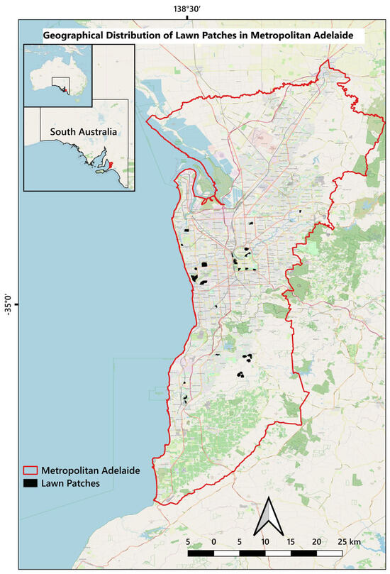
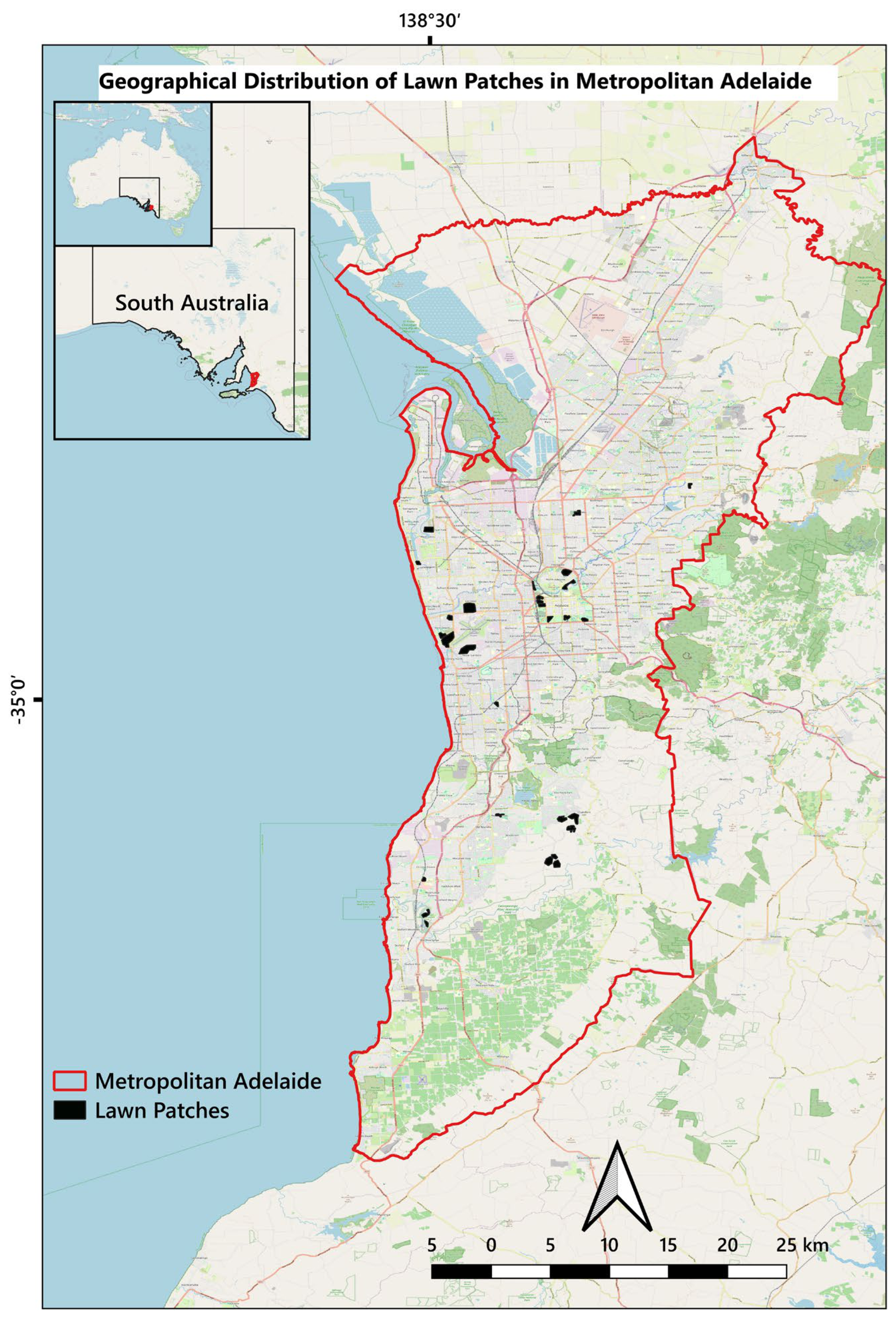
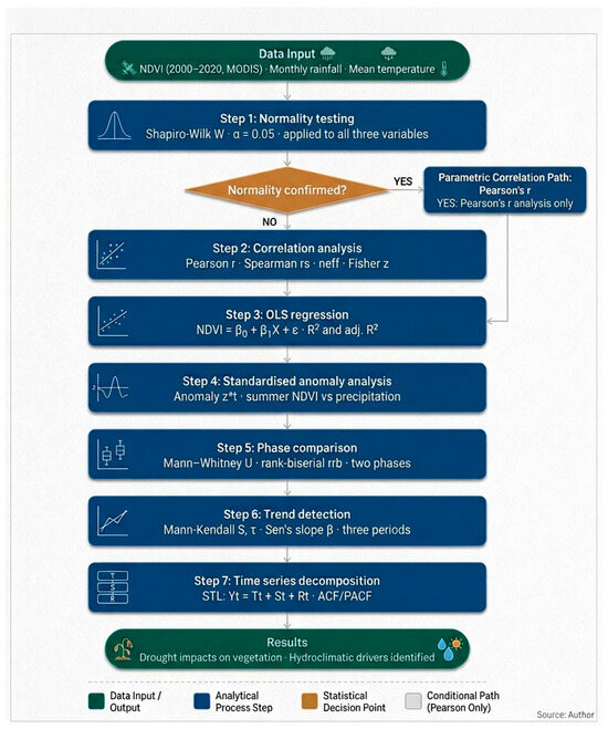
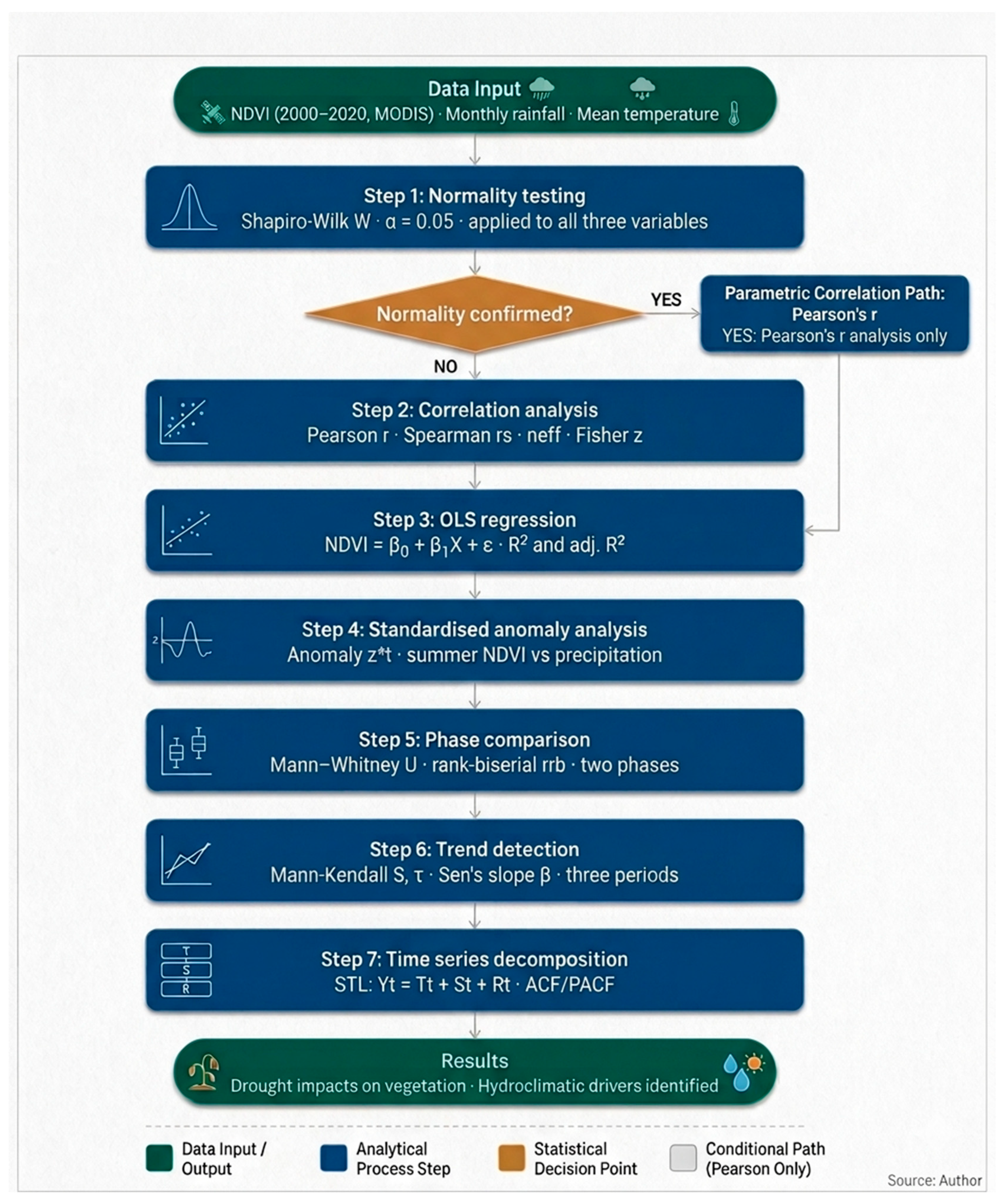
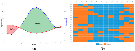
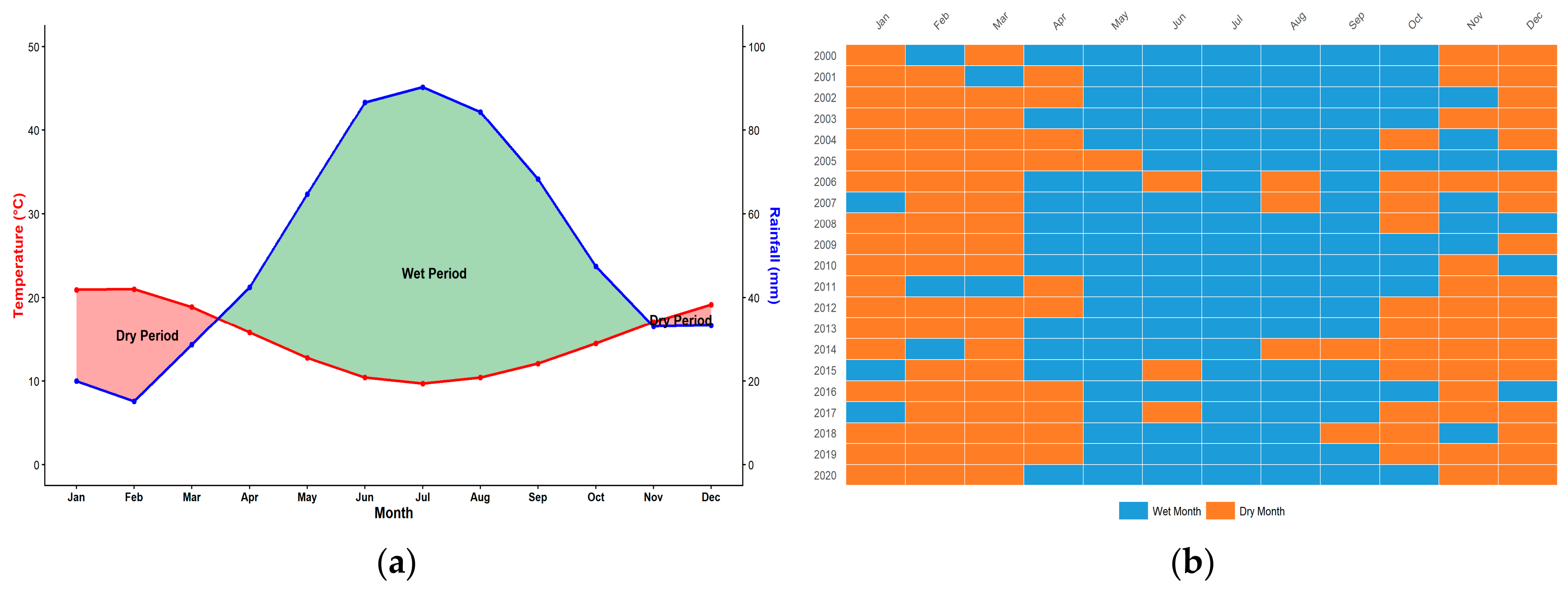
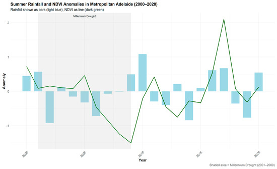
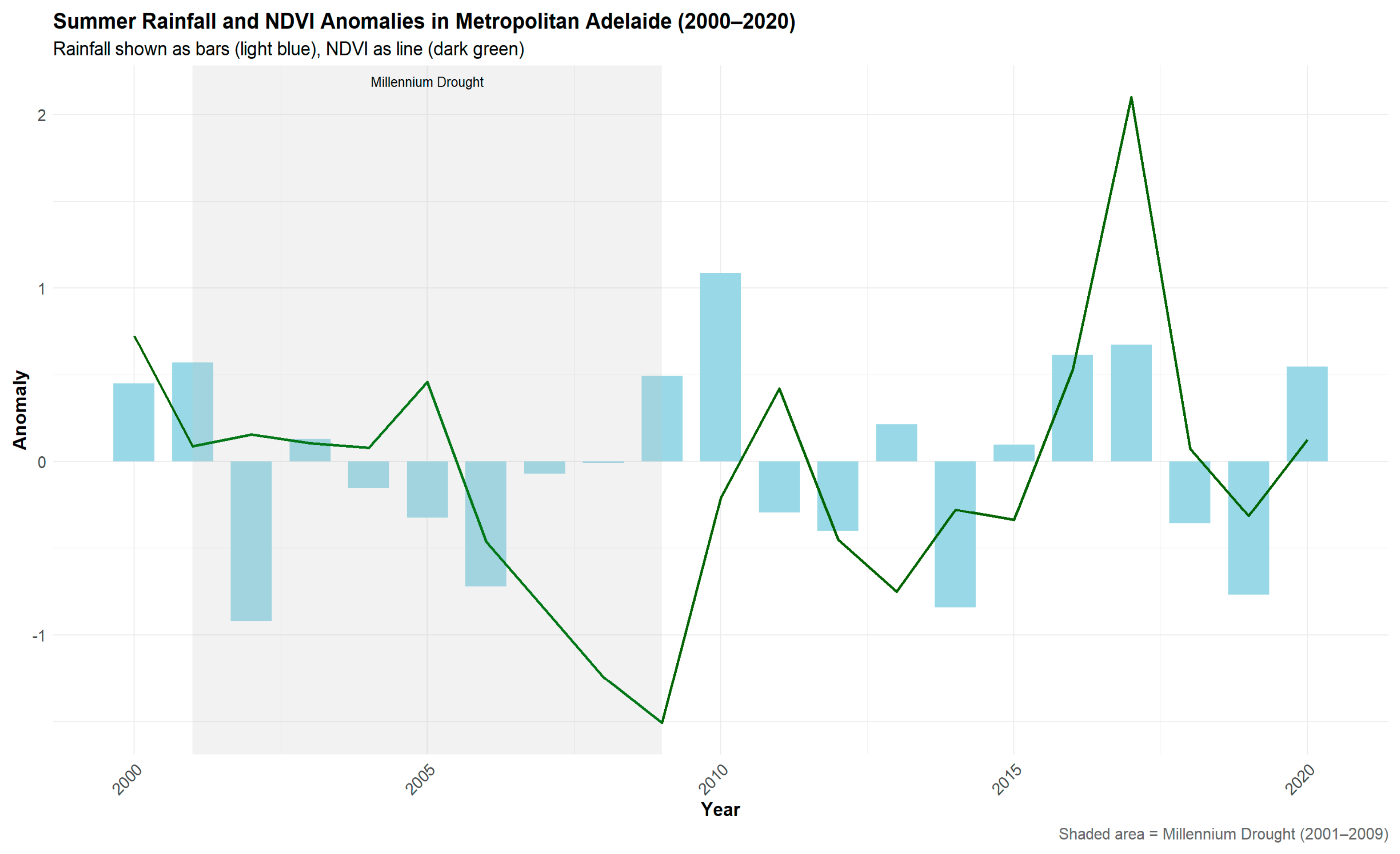
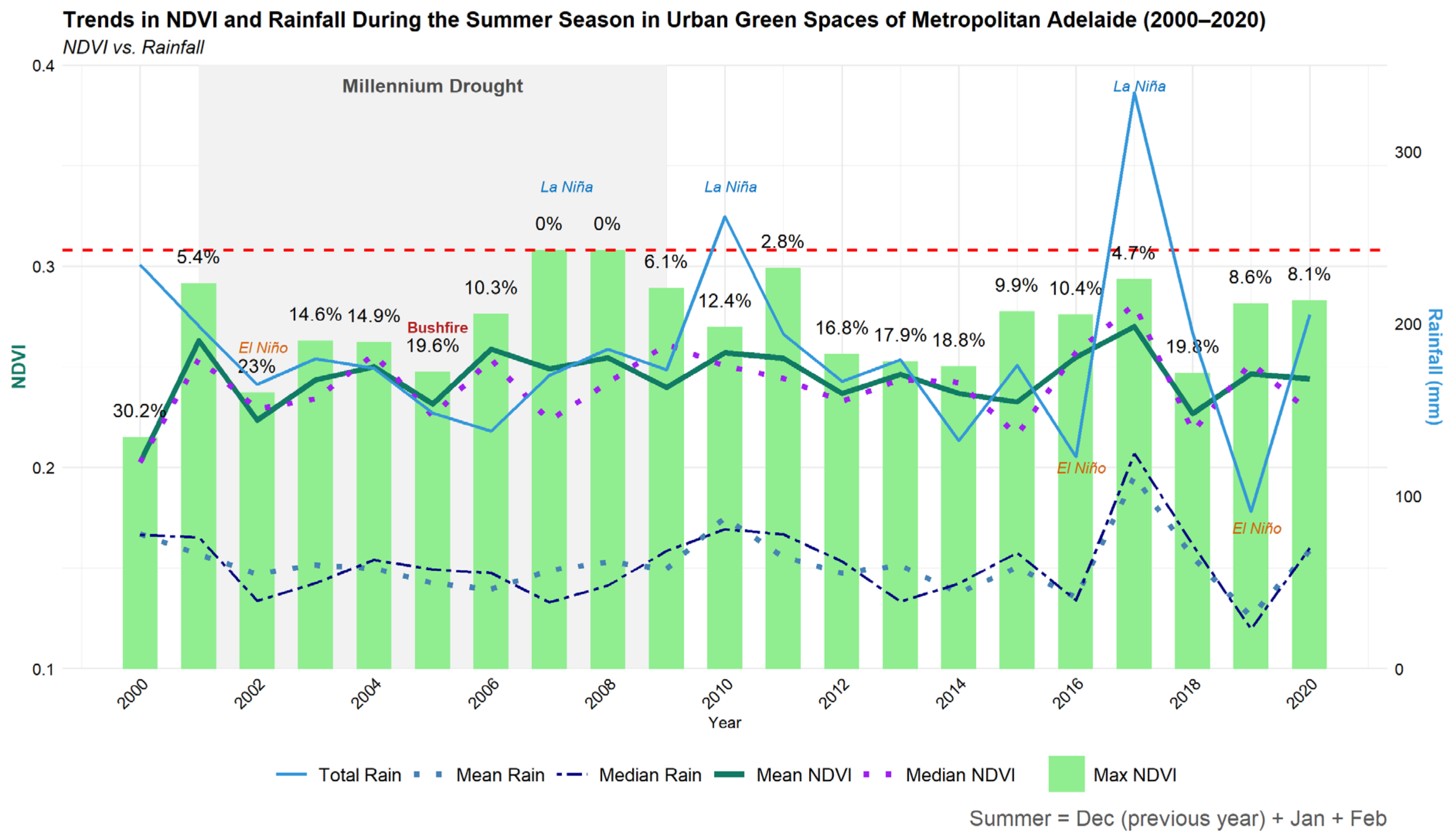
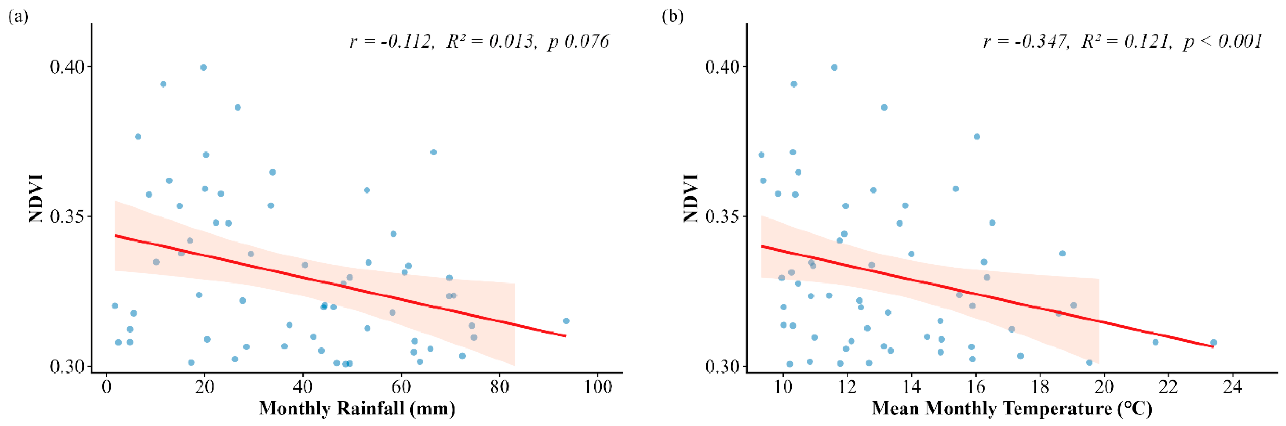
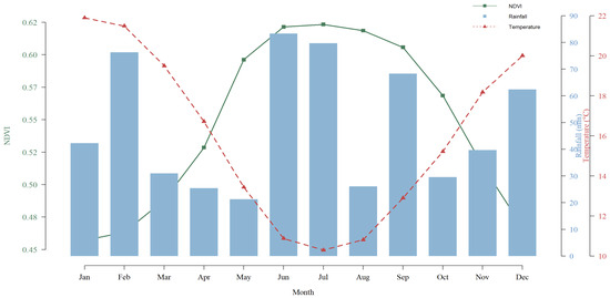
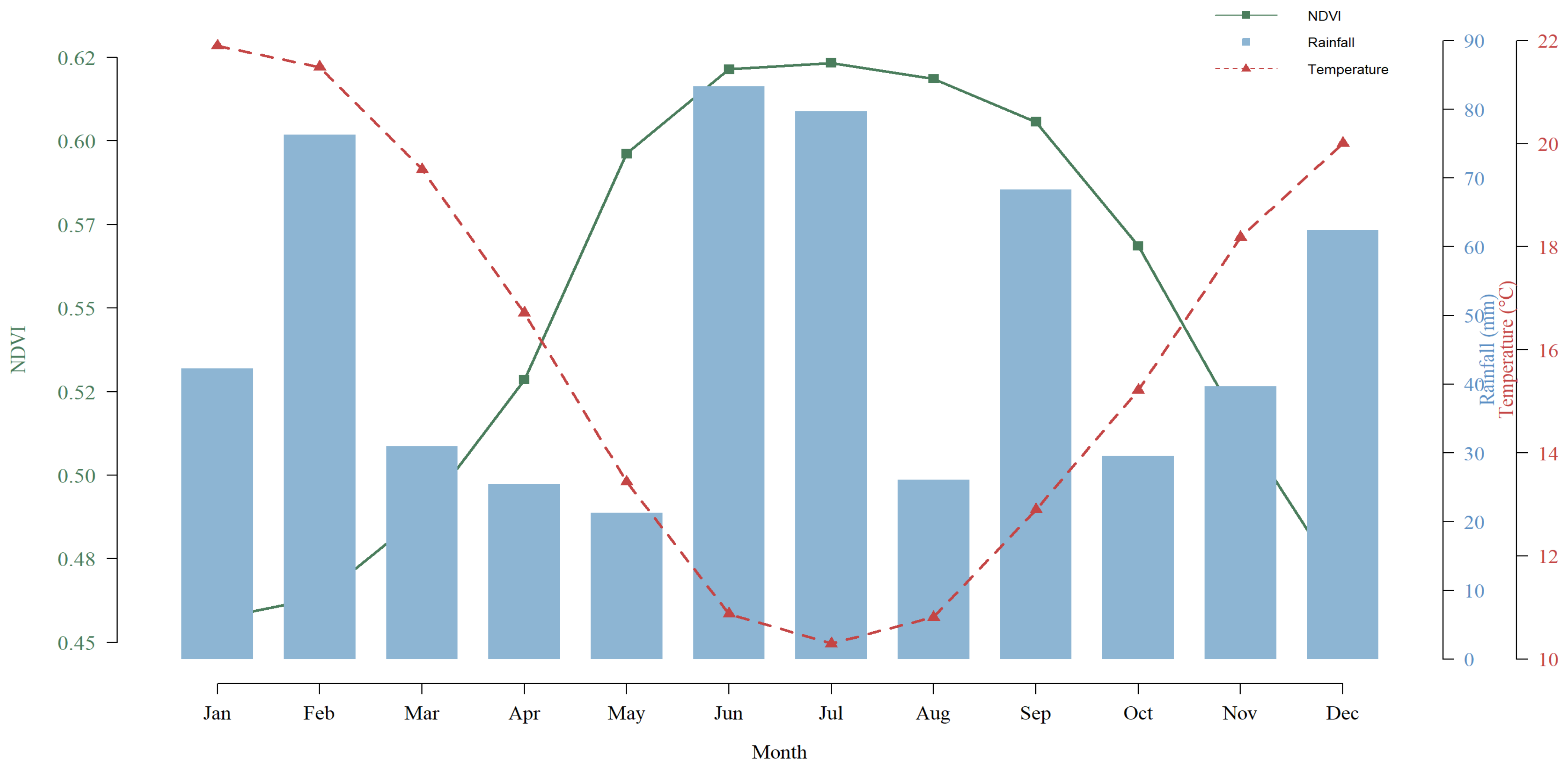
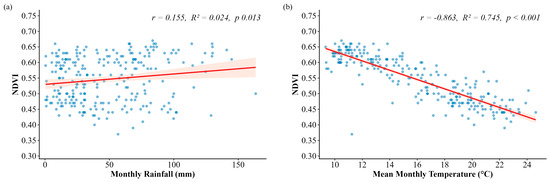
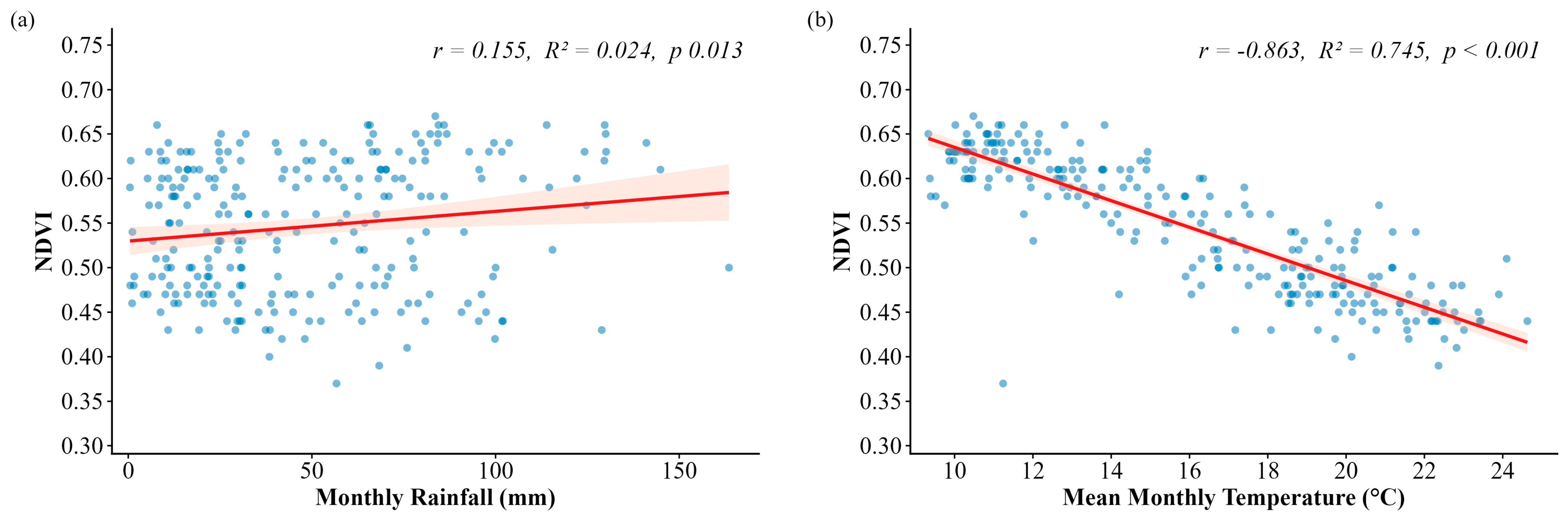
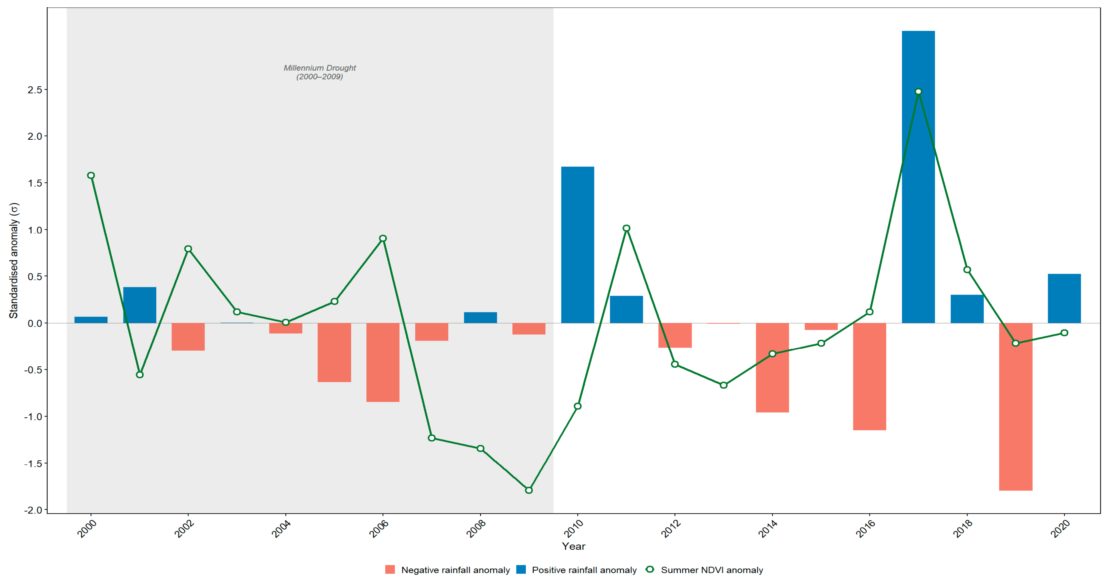
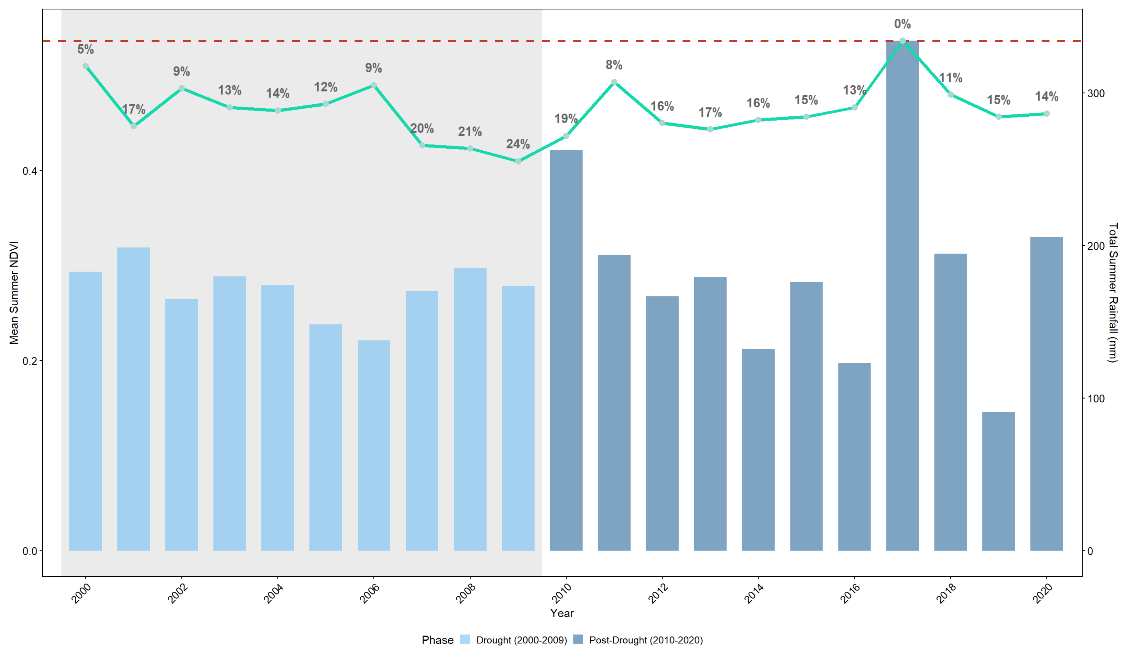
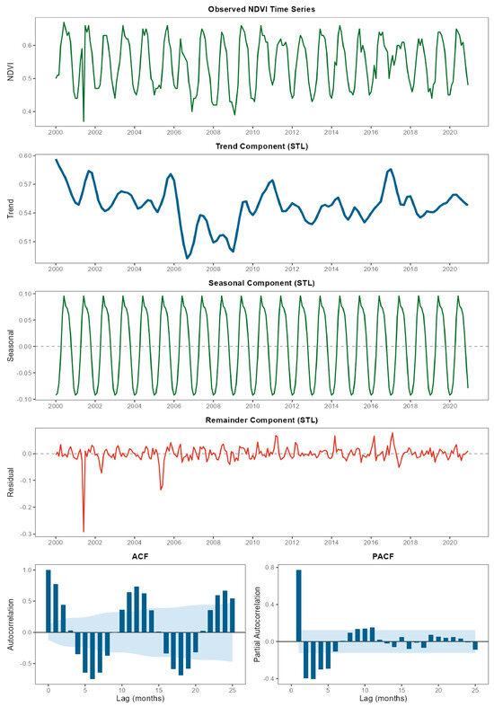
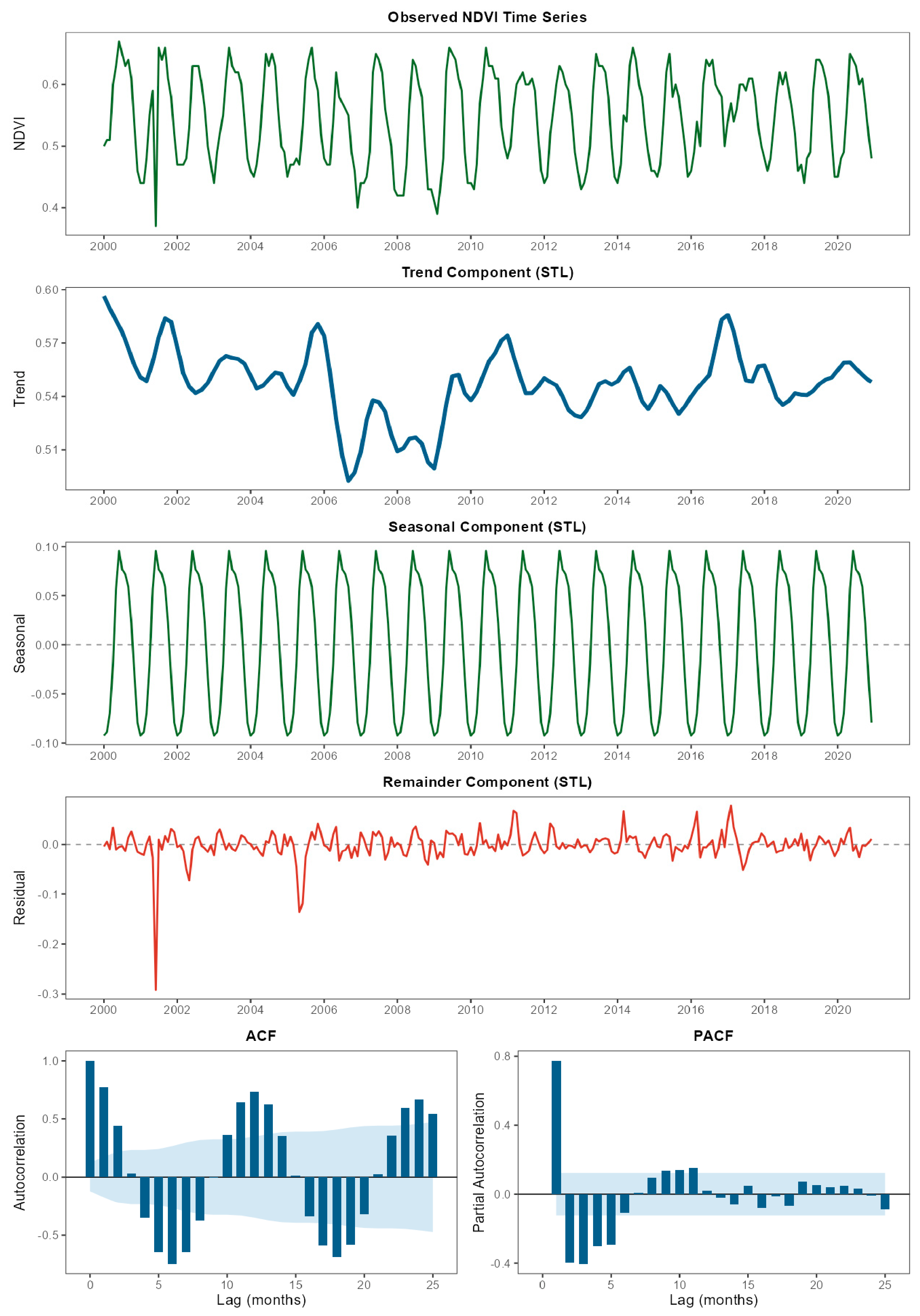

Disclaimer/Publisher’s Note: The statements, opinions and data contained in all publications are solely those of the individual author(s) and contributor(s) and not of MDPI and/or the editor(s). MDPI and/or the editor(s) disclaim responsibility for any injury to people or property resulting from any ideas, methods, instructions or products referred to in the content. |
© 2026 by the authors. Licensee MDPI, Basel, Switzerland. This article is an open access article distributed under the terms and conditions of the Creative Commons Attribution (CC BY) license.