1. Introduction
Time series are currently used for recording dynamic systems in various situations, such as factory control, power demand, health monitoring and environmental observation [
1,
2]. Remote sensing provides a special form to this problem. Satellites and air-borne sensors repeatedly observe the same area; thus, the obtained data show information about vegetation cycle, land-use changes, hydrological variations, urban expansion and unusual environmental phenomena. AutoRegressive Integrated Moving Average (ARIMA), exponential smoothing and Kalman filtering are still useful reference methods since their assumptions are clear and their results can be easily inspected [
3,
4]. However, these assumptions become weak in most of the present Earth observation archives. Factors like cloud cover, errors in atmospheric correction, different revisit times, sensor offsets and complex interactions among spatial, spectral and temporal aspects frequently result in nonlinear, non-stationary and multi-dimensional sequences [
5,
6]. With the continuous increase in Landsat, Sentinel, Moderate Resolution Imaging Spectroradiometer (MODIS) and similar archives, the issue of model building is not only how to fit a smooth curve, but also how to preserve the significant temporal structure under imperfect observation conditions [
7].
Neural networks have extended the types of patterns obtained from both general time series and satellite image time series (SITS). Recurrent neural networks (RNNs), long short-term memory networks (LSTMs), temporal convolutional networks (TCNs), and attention-based Transformers have been applied in land-cover classification, change detection, estimation of biophysical parameters, forecasting, missing value recovery and abnormality detection [
8,
9,
10,
11,
12]. In Earth observation data, their advantages are obvious: seasonal variations, disturbed events and cross-band or cross-sensor relationships can all exist in one long record. However, the evidence from these studies is not consistent. It is hard to transfer when the observations are from different sensors, the sampling is irregular, some values are missing or polluted with clouds, and the model results should still be understandable in physical aspects [
6,
13].
Another bottleneck is the fixed interface used by many deep time-series models. A change in sequence length, prediction horizon, variable set, or sampling interval can require a new head, a different architecture, or retraining. This is already inconvenient in general benchmarks, and it is more severe in remote sensing, where the record length and acquisition rhythm vary by sensor, region, spatial resolution, and orbit schedule. Missing observations and modality gaps are part of the data, not rare exceptions. Operational monitoring systems may combine optical, radar, thermal, and ancillary environmental streams whose noise properties differ from one another. A foundation model for this setting therefore has to spend capacity according to the local behavior of the sequence, rather than forcing every segment through the same computation.
The move toward time-series foundation models has begun to address some of these issues. TimeGPT-1 [
14], Timer [
15], Lag-Llama [
16], and TimesFM [
17] indicate that large-scale pretraining can make temporal representations more transferable. Sparse Mixture-of-Experts (MoE) layers add another route by increasing model capacity while activating only part of the network for each input [
18,
19]. Still, temporal heterogeneity is only partly handled. Stable trends, noise bursts, abrupt changes, and long-range dependencies are often passed through much the same computational route. In remote sensing this is a poor match to the data, because smooth seasonal cycles can sit next to cloud artifacts, missing values, or disturbance events in the same sequence. The field also still needs stronger adaptation across sequence lengths, horizons, variables, and sampling intervals, together with pretraining data broad enough to cover industrial, scientific, and Earth observation regimes.
Here, we introduce TimeHome as a universal foundation model for heterogeneous time series. We make two main choices in its design. First, the Heterogeneous Mixture-of-Experts (H-MoE) module routes tokens to functionally different experts—zero, masked, and low-rank experts—using a learnable temperature-controlled gate. This lets the model handle stable intervals, noisy observations, and more complex temporal transitions with different operations. Second, the hybrid local–global attention module combines short-window context with global memory tokens, so local changes and longer seasonal or environmental dependencies are represented together. For scalability, low-rank factorization is used in both the experts and the gate, and dynamic expert pruning also disables rarely used experts during inference.
TimeHome is pre-trained on TS-200B, a heterogeneous corpus built to expose the model to several temporal domains and resolutions before downstream evaluation. We then test it on forecasting, imputation, anomaly detection, zero-shot and few-shot transfer, a remote sensing extension, ablations, domain sensitivity, and efficiency. Across these experiments, TimeHome keeps one backbone for multiple tasks while improving accuracy or cost in several benchmark settings. The main contributions are:
We design an H-MoE architecture in which zero, masked, and low-rank experts are selected by a temperature-scaled gate, so the active expert set changes with the sequence context and input complexity.
We factorize both expert and gating modules into low-rank forms, reducing parameters and computation while retaining the capacity required by long temporal records.
We use variational dropout to regularize long-range attention links, and combine local temporal windows with global dependency modeling in a hybrid attention mechanism.
We use TS-200B pretraining with task-specific heads for forecasting, imputation, and anomaly detection, and apply dynamic expert pruning to reduce inference cost with limited accuracy loss.
2. Materials and Methods
2.1. Literature Review and Research Gap
2.1.1. Classical Methods of Time-Series Analysis
Classical time-series analysis is still based on statistical models like AutoRegressive Integrated Moving Average (ARIMA), Exponential Smoothing (ETS) and Kalman filters [
3]. Its advantage is not only that it can be precise in simple situations, but also that its assumptions are clear: the trends, seasonal components and short-term correlations can be easily detected when the signal is nearly linear and stationary. Remote sensing has applied similar modeling and decomposition techniques for the retrieval of vegetation phenology, seasonal trend analysis and land surface change monitoring; TIMESAT, Breaks For Additive Seasonal and Trend (BFAST), Landsat-based Detection of Trends in Disturbance and Recovery (LandTrendr) and Continuous Change Detection and Classification (CCDC) are typical examples [
20,
21,
22,
23]. Spectral Analysis [
24] provides a frequency-domain perspective, whereas Multiple Seasonal-Trend decomposition using Loess (MSTL) [
25] and Theta [
26] are frequently used when the seasonal forecasting problem can be divided into regular components. For vegetation indices, land surface phenology, surface temperature and hydrological variables which show clear cycles, these models are still valuable benchmarks.
Linearity, Gaussian noise and stationarity are assumed to simplify the problem, but they do not allow for long-term dependencies, sudden changes in conditions and uncertainties from various sources. Their limitations become apparent when the data deviate from this assumption. The discrepancies are more evident in remote sensing since the same dataset may include cloud interference, atmospheric effects, irregular observation times, missing observations and inconsistencies among different sensors [
23,
27,
28]. Moreover, the classical methods usually treat each series individually which is not suitable for the Earth observation data, where the spectral bands, adjacent areas and different sensing modes are related and should be considered together.
Machine learning techniques, such as gradient-boosted decision trees like XGBoost [
29] and LightGBM [
30], can deal with some of these assumptions and are appropriate for the regression estimation of structured data. However, the main difficulty lies in the preprocessing of the data prior to the model training. Usually, several manually designed descriptors, including temporal summaries, spectral indices, lag features etc., affect the final outcome. In remote sensing, the reliance on feature creation needs more flexibility when the environment, sensor or acquisition method changes. Some recent research has focused on the study of neural time-series forecasting and various sequence models [
31].
2.1.2. Deep Learning-Based Methods
Deep learning modifies the time-series toolbox since it extracts temporal patterns from data directly rather than from pre-defined decompositions. This is important in remote sensing as the observation records usually include seasonal variations, disturbance events, heterogeneous information from different sources and spectral–spatial–temporal associations. Research on satellite image time series (SITS) indicates that temporal convolutional neural networks (CNNs), self-attention encoders and spatio-temporal transformers can assist in land-cover mapping, crop surveillance and segmentation [
8,
32,
33,
34]. By taking inspiration from natural language processing [
35] and computer vision [
36], these neural structures have also been applied to forecast [
11], classify [
37], estimate missing values [
38] and detect abnormal changes [
39]. In the field of remote sensing, these functions are equivalent to environmental prediction, study of land-cover changes, interpolation of missing values in satellite sequences and identification of unusual phenomena in long monitoring records.
Early neural methods used Recurrent Neural Networks, such as LSTM [
40] and gated recurrent unit (GRU) [
41,
42], to transmit information through gated temporal states. DeepAR [
9] and the exponential smoothing-recurrent neural network (ES-RNN) [
10] are typical prediction models in this field. For example, DeepAR predicts the future based on the observed history and shared latent dynamics; thus, the recurring patterns in related sequences can be applied [
9]. Similarly, the reasoning also exists in remote sensing architectures like DuPLO, which combines convolutional and recurrent streams to make use of both spatial and temporal cues in SITS classification [
43]. However, the main disadvantage is the scalability problem: it is difficult to parallelize the recurrent models for a great amount of data, and long-range gradients are hard to preserve.
Transformer-based methods deal with some of the costs by utilizing self-attention to establish direct connections between distant time steps and to process multivariate inputs more flexibly. In remote sensing, PSE+TAE, U-Net with Temporal Attention Encoder (U-TAE), Temporo-Spatial Vision Transformer (TSViT) and the later set-based temporal encoders obtain good performance in classification and dense prediction under irregular acquisitions and complicated seasonal variations [
28,
32,
33,
34]. However, most models are still trained for a single task, require labeled data and fail to maintain their reliability when the sensor, region or acquisition conditions vary. This suggests the need for pre-trained time-series models with wider applicability.
2.1.3. Heterogeneous Temporal Data Modeling
Heterogeneous temporal data widely exist in both general time-series applications and remote sensing scenarios. Such heterogeneity may come from different temporal resolutions, irregular sampling intervals, missing observations, sensor-specific noise, modality gaps, non-stationary dynamics, and the coexistence of smooth trends, high-frequency fluctuations, and abrupt changes. In remote sensing, these issues become more pronounced because Earth observation records are often collected from different sensors, regions, seasons, and acquisition conditions, leading to complex temporal and cross-source variability.
Existing studies have addressed heterogeneous temporal data from several perspectives. One line of work focuses on multi-source and multimodal temporal fusion. For example, remote sensing methods combine optical, synthetic aperture radar (SAR), and other observation streams to exploit complementary information across sensing modalities [
13]. Hybrid architectures such as DuPLO further combine convolutional and recurrent streams to jointly capture spatial and temporal cues in satellite image time series [
43]. Another line of work aims to model irregular and variable-length temporal observations. Temporal attention and set-based encoders, such as PSE+TAE, U-TAE, TSViT, and later satellite image time-series encoding methods, have been developed to handle irregular acquisitions and complex seasonal dynamics in satellite image time series [
28,
32,
33,
34]. In addition, cloud-contaminated or incomplete observations have motivated sequence-to-sequence reconstruction and gap-filling methods for optical satellite time series [
27].
Outside remote sensing, temporal heterogeneity is often handled through decomposition, frequency-domain modeling, stationarity modeling, or multi-scale representations. Decomposition-based models separate trend and seasonal components, frequency-enhanced models emphasize periodic structure, and temporal-variation models describe multi-period dynamics at different scales [
4,
12,
44,
45]. These designs are useful when the source of variation is known in advance. They become less reliable when several problems occur together, such as noisy observations, missing values, heterogeneous regimes, and cross-domain distribution shift.
Taken together, prior work offers useful tools for particular aspects of heterogeneity: multi-source fusion, irregular sampling, reconstruction of missing observations, seasonal decomposition, and multi-scale modeling. What is still missing is a unified mechanism that can change its modeling behavior inside the same sequence. Most existing architectures either target one task or use homogeneous computation for all temporal patterns. TimeHome addresses this gap with H-MoE, where functionally different experts provide separate inductive biases for stable trends, noisy fluctuations, and complex temporal transitions within one foundation-model framework.
2.1.4. Time-Series Foundation Models
Foundation models in language and vision have encouraged similar work on time-series understanding [
46]. The common idea is to pre-train on diverse temporal data and reuse the learned representation for forecasting, classification, anomaly detection, and other tasks with little task-specific supervision. Remote sensing is a natural test case for this idea because temporal, multispectral, and multimodal Earth observation archives are already large and varied; SatMAE, EarthPT, and SkySense illustrate this broader pretraining trend [
47,
48,
49]. The attraction is clear: one model could help bridge regions, sensors, resolutions, and acquisition conditions that are otherwise treated separately.
The difficulty lies in the fact that remote sensing time series are not only similar to language sequences with a different vocabulary. They often have non-stationarity, irregular sampling, missing data, atmospheric influence and differences among sensors [
23,
27,
28]. Therefore, a representation which is suitable for one sensor or area may not be applicable to environmental monitoring, study of land cover changes, reconstruction of missing values or detection of anomalies in other places. A good basic model for Earth observation should deal with temporal heterogeneity, multi-modality and domain shift explicitly rather than considering that scale is enough to solve these problems.
(1) Single-Modality Foundation Models: At present, most time-series fundamental models are mainly based on numerical time data and are mostly applied for prediction. Lag-Llama [
16] and TimeGPT-1 [
14] are the early examples of transformer networks pre-trained on a large quantity of time-series data. Lag-Llama includes lag variables as extra explanatory factors, whereas TimeGPT-1 uses a multi-layer transformer to deal with different forecasting durations. Some subsequent models have extended their range and the fields of application: TimesFM [
17] adopts a decoder-only approach, Tiny Time Mixers (TTM) [
50] applies the TSMixer framework and Moirai [
51] integrates masked modeling in a universal transformer which is trained on the Large-scale Open Time Series Archive (LOTSA), an accumulated dataset consisting of 27 billion observations from nine different categories. The diffusion type models such as TimeGrad [
52] and TransFusion [
53] also include a generating part by learning to transform noise into reasonable time sequences through variational inference.
(2) Multimodal and LLM-Augmented Models: Another field of work includes the use of language or signal modalities in time-series modeling. Time-LLM [
54] modifies the temporal inputs through reprogramming with a pre-trained large language model and Multimodal ECG-Text Self-supervised pre-training (METS) [
55] links a trainable electrocardiogram (ECG) encoder with a stable language model for paired biomedical signals and clinical narratives. In contrast, prompt-based methods have a different way of processing. PromptCast [
56] converts numerical sequences into language prompts to accomplish forecasting, similar to sentence-to-sentence generation, so that an ordinary language model can be used as a predictor. GPT4MTS improves upon this idea by incorporating both numerical and textual inputs into a single language model framework [
57]. These studies show the application of language and time interaction, but also reveal some unsolved issues: the continuous values must be transformed into discrete tokens, the temporal relationship needs to be maintained and the generated outcomes should keep numeric accuracy. A recent survey provides a more detailed introduction to the time-series models based on language models [
58].
(3) Model Scaling via Mixture-of-Experts (MoEs): MoE models are attractive since they enlarge the parameter capacity without fully activating the network for each input [
59,
60]. In terms of time series, there exist light versions like Mixture-of-Linear-Experts for long-term prediction [
61]. Compared with TimeHome, the main difference lies in the type of expert specialization. For instance, Time-MoE [
18] and MoE++ [
19] mainly employ homogeneous experts, which have the same dense feedforward network structure. This can enhance the model’s ability to handle capacity, but it limits the router’s options in distinguishing a stable trend from noise or an unexpected change. TimeHome, on the other hand, utilizes experts with different functions: Zero Experts for simple stability, Masked Experts for noise reduction, and Low-Rank Experts for feature extraction. Moreover, it substitutes the usual dense gating with a low-rank gating network and performs dynamic expert pruning at the time of inference. These modifications are intended to reduce the latency and the number of active parameters, which become significant issues in large-scale or constrained environments.
In conclusion, most of the existing models focus on either task-specific optimization or parameter scaling. For this reason, TimeHome integrates unified pretraining, heterogeneous MoE routing and efficiency-oriented design to ensure that general-purpose time-series modeling is still flexible and applicable.
Table 1 lists the main advantages and disadvantages of the mentioned representative models.
2.2. Overall Architecture
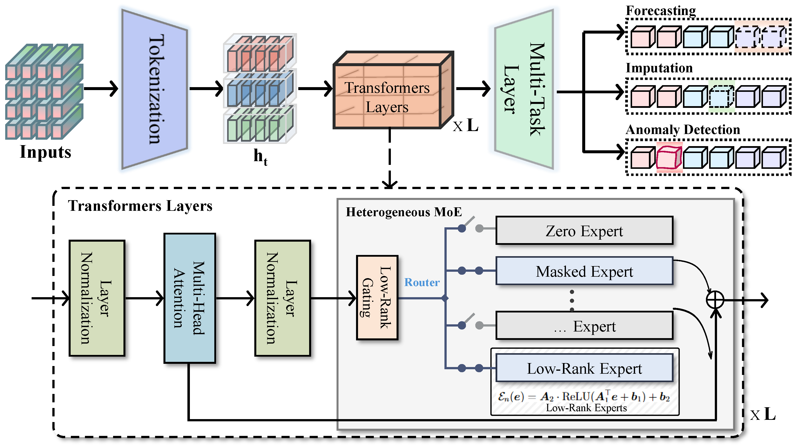
Figure 1 gives the architecture. TimeHome targets multivariate, long-range, and irregular time series, where a single dense computation path can spend unnecessary effort on simple intervals and still miss local regime changes. The backbone first builds multi-scale context with hybrid local–global attention, then uses a heterogeneous sparse Mixture-of-Experts (H-MoE) layer to route tokens to different expert operations. Low-rank factors are used in both the experts and the gate to reduce parameter count and inference cost.
Table 2 lists the notation used in the
Section 2.
For an input sequence, the forward pass can be read as four steps. Raw scalar or multivariate observations are projected into latent temporal tokens. The attention module enriches each token with local-window information and global-memory context. The H-MoE router then selects a small group of functionally distinct experts for each token representation. Their weighted outputs are passed to task-specific heads for forecasting, imputation, or anomaly detection.
Input Layers and Tokenization. The input layer converts raw time-series values into token representations for the transformer backbone (Algorithm 1). We use point-wise linear projections so that temporal order is retained before attention is applied. For each input token, the gated linear unit produces
through the component-wise product of three projections:
where
and
. Here,
is the sigmoid function used in the Swish activation,
, and
are learnable parameters with channel dimension
D. The multiplicative gate filters or amplifies features at each time step before the sequence enters the attention layers. For multivariate inputs, a sensor set
is embedded by stacking or jointly projecting sensors with shared linear weights and learnable fusion weights. This keeps a common temporal representation while preserving inter-variable differences [
62].
| Algorithm 1 TimeHome Pipeline (Section 2.2) |
Input: Historical sequence , L layers with N experts
- 1:
Initialize input embedding via Equation ( 1) - 2:
for to L do - 3:
Compute relevance scores via Equation ( 5) - 4:
Compute MoE gating weights via Equation ( 8) - 5:
Select top-S experts based on gating weights - 6:
for to S do - 7:
Compute heterogeneous expert via Equation ( 7) - 8:
end for - 9:
Output via Equation ( 9) - 10:
end for - 11:
Generate from final embeddings
Output: Prediction for downstream tasks |
Hybrid Local–Global Attention. Real-world time series often contain short-lived fluctuations and long-range trends in the same sequence. TimeHome thus uses two attention paths. The local branch attends within a sliding window and captures short-term changes. The global branch uses representative memory tokens, either learned or sampled, to carry longer-range context and rare events. A learnable gate fuses the two outputs for each query token, so the effective context range can change with the input.
For each query token
, the local attention is computed over a fixed-size window
:
where
denotes the local attention weight by scaled dot-product.
In parallel, a global attention path incorporates a set of representative memory tokens
, obtained either through learnable global tokens or periodic sampling from the sequence. This component supports long-range dependency modeling:
To adaptively fuse the local and global attention branches, the final attention output is obtained through a learnable scalar gate. To avoid circular dependency in the gate computation, the fusion weight is computed directly from the outputs of the local and global attention branches:
where
denotes feature concatenation,
and
are learnable parameters, and the relative contribution of local and global contexts is controlled by
. The fused attention representation is computed as:
Variational Attention Dropout. We add distance-aware variational dropout to regularize long-range attention. Instead of applying a fixed dropout rate to all attention links, the dropout probability changes with temporal distance. This encourages the model to suppress weak or redundant long-range links while retaining connections that carry useful temporal context. A dropout mask
is applied to each attention link:
where
denotes a learnable embedding of the absolute time lag [
63,
64].
Heterogeneous MoE. A standard MoE layer routes an input to a small subset of expert subnetworks and combines their outputs with learned gating weights. TimeHome keeps this sparse routing principle but changes the expert space. Rather than using experts with identical feedforward network (FFN) structures,
contains
N experts
with heterogeneous residual operations. Given
, the
n-th expert is written as:
contains zero, mask, and linear operations. The zero operation removes the residual heterogeneous term and preserves the FFN output. The mask operation applies a random zero mask to
of channels. The linear operation uses a learnable projection on the expert output. These operations give the router different inductive biases: the zero expert preserves stable or slowly varying segments, the masked expert suppresses unreliable local responses, and the low-rank expert models trend changes, abrupt transitions, and long-range dependencies. In this sense, H-MoE is a structurally specialized routing layer rather than only a larger pool of FFNs.
A trainable gating network
assigns weights to experts from the input representation
. We use a temperature-scaled softmax:
where
is the gating weight matrix,
is optional noise for load balancing, and
is annealed during training. To limit computation, only the top-
S experts are selected (
). The final output
is a weighted sum of selected expert outputs:
where
are omitted for notational simplicity. The layer limits active computation through top-
S routing while allowing different expert operations to be selected for different temporal patterns.
End-to-end workflow. Algorithm 1 summarizes the complete path from input tokenization to attention, routing, and prediction. The main hyperparameters, including the number of experts
N, low-rank dimension
r, and pruning threshold
, are reported in
Section 3.1.
2.3. Low-Rank Expert and Gating Design
As the expert pool grows, dense expert and gating matrices can dominate memory and computation. TimeHome therefore represents both expert weights and gating parameters in low-rank form. The goal is to reduce parameter count and floating-point operations (FLOPs) while keeping enough capacity for long sequences and resource-constrained inference.
Low-Rank Expert Networks. In traditional MoE implementations, each expert
typically consists of a fully parameterized feedforward network (FFN) with dense weight matrices. To improve parameter efficiency, we replace this with a low-rank approximation of the hidden-layer transformations. Specifically, using the rectified linear unit (ReLU) activation, the standard FFN mapping
is replaced by a rank-
r approximation:
where
, and
is the low-rank dimension. This factorization reduces both the parameter count and the complexity from
to
per expert. As a result, the model becomes more suitable for large-scale deployment with minimal performance degradation.
Low-Rank Gating Network. Complementing the low-rank expert design, we introduce a low-rank gating mechanism that enhances the efficiency of computing expert logits for dynamic routing. Instead of using a dense projection:
the gating logits are computed through a low-rank factorization:
followed by temperature-scaled softmax to obtain the expert assignment distribution:
This factorization cuts trainable parameters and inference-time FLOPs, especially when the expert count
N or feature dimension
D is large. The expert modules and the gate are still trained end-to-end inside TimeHome. In the experiments, this low-rank design [
65] keeps predictive performance close to the full form while reducing memory use and inference time, a practical requirement for long-horizon forecasting.
2.4. Output Layers
TimeHome retains one transformer backbone and connects light heads to the downstream tasks. Each head is a single-layer FFN with its own loss, thus enabling forecasting, imputation and anomaly detection to use the same learned representation without changing the backbone.
Time-Series Forecasting. For a historical sequence
, the forecasting head predicts the next
M values,
:
where
denotes the last-token representation from the final layer. We train this head with mean squared error (MSE) against the ground truth:
Time-Series Imputation. For a partially observed sequence
, the binary mask
marks observed values with 1 and missing values with 0. The imputation head predicts values at every time step:
The loss is evaluated only at masked positions:
Time-Series Anomaly Detection. For anomaly detection, the head reconstructs the input sequence and uses reconstruction deviation as the anomaly signal. With
, the score at time step
t is:
The score can be thresholded, for example by statistical quantiles or learned calibration, to flag anomalous
. The detection loss uses reconstruction error:
Thus, the heads differ only in their output projection and loss. The shared backbone keeps the multi-task setting compact, while the heads still provide task-specific supervision.
2.5. Dynamic Expert Pruning During Inference
To reduce inference cost, TimeHome uses Dynamic Expert Pruning. During training, the model records how often each expert receives non-negligible routing weight. Experts that remain rarely used are disabled at inference time, reducing active parameters and latency without retraining.
Let
denote the full set of
N experts. Let
be the corresponding gating weights for input token
t. During training, we estimate the average activation rate for each expert as:
where
indicates how frequently expert
n is selected or contributes to the output. We define a pruning threshold
, and set
based on preliminary validation. This value provides a good trade-off between accuracy and pruning ratio.
During inference, we discard expert
if its average activation
is below the threshold, i.e.,
. The resulting active expert set at inference time is:
This pruning strategy reduces memory use and computation in multi-task deployments. It does not require fine-tuning or weight modification and can be applied on a per-task basis.
To maintain consistency in expert routing, the gating distribution is renormalized over the reduced expert set:
This procedure is compatible with top-S sparse activation and is intended for resource-constrained or real-time deployment settings.
2.6. Self-Supervised Label Construction and Pre-Training Objectives
The pre-training protocol does not rely on manual annotations. TimeHome derives supervision from the raw series by viewing each sequence from different temporal angles. The future segment provides a target for trajectory prediction, masked observations provide targets for imputation, and the full input sequence provides the reference for reconstruction-based anomaly modeling. These three pretext tasks are optimized through task-specific heads attached to the shared TimeHome backbone.
Labeling strategy. TimeHome generates pseudo-labels from the observed temporal order. For forecasting, the segment after the input context is used as the target. For imputation, observed values are randomly masked, and their original values become reconstruction targets. For anomaly modeling, the sequence is reconstructed from its latent representation, and the later reconstruction deviation is converted into an anomaly score. The labeling strategy is therefore a form of temporal self-labeling based on ordering and continuity rather than external annotation.
Pretext task 1: future trajectory prediction. Given a historical context
, TimeHome predicts the horizon
. The observed future values serve as pseudo-labels:
The forecasting objective is defined as:
This objective makes the backbone learn temporal evolution, including trend, periodicity, and long-range dependency structure.
Pretext task 2: masked value reconstruction. For imputation-oriented pre-training, a binary mask
is applied to the input sequence, where
denotes an observed value and
denotes a masked value. The head reconstructs the original values hidden by the mask:
The masked reconstruction loss is:
Only masked positions contribute to this objective, so the model must infer the hidden values from nearby temporal evidence and longer sequence-level regularities.
Pretext task 3: reconstruction-based anomaly modeling. For anomaly-aware representation learning, TimeHome reconstructs the input sequence from the latent representation:
The reconstruction loss is formulated as:
During inference, the point-wise reconstruction error is used as the anomaly score:
A larger reconstruction error indicates a stronger departure from the normal dynamics learned during pre-training.
Overall objective. The overall self-supervised pre-training objective is defined as:
where
,
, and
are task-balancing coefficients. By combining temporal continuation, contextual reconstruction, and distributional regularity, the objective encourages transferable representations from unlabeled time series.
2.7. Large-Scale Time-Series Data for Pre-Training
Large-scale and heterogeneous pre-training data are essential for building a transferable time-series foundation model. In contrast to prior work [
11,
18], which primarily relies on task-specific benchmarks, we construct TS-200B as a large-scale corpus to expose TimeHome to diverse temporal dynamics, sampling patterns, missing-value structures, and domain variations before downstream adaptation.
Data sources and domain composition. TS-200B aggregates time-series records from multiple public and real-world sources [
66,
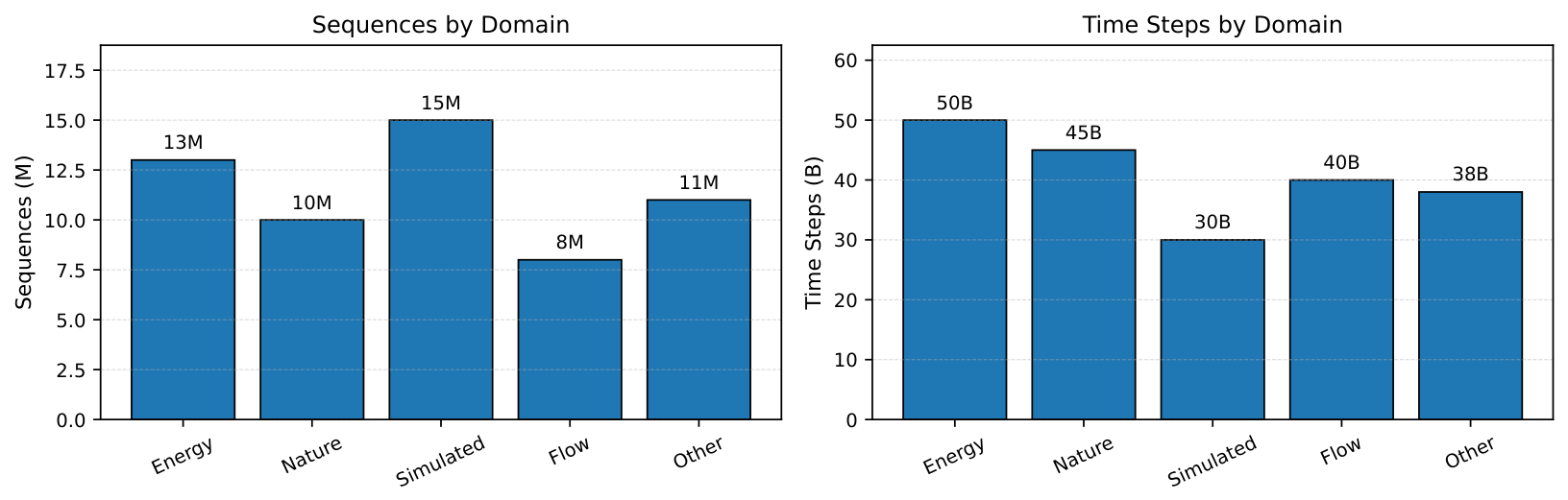
67]. The corpus covers five major domains: Energy, Nature, Simulated, Flow, and Other. These domains are selected to reflect diverse temporal behaviors, including periodic consumption patterns, environmental variations, synthetic controlled dynamics, traffic or flow-related changes, and miscellaneous industrial or scientific signals. According to
Table 3, the TS-200B consists of 57 million sequences and 203 billion validated time steps. In detail, the Energy domain has 13 million sequences and 50 billion time steps; the Nature domain has 10 million sequences and 45 billion time steps; the Simulated domain includes 15 million sequences and 30 billion time steps; the Flow domain has 8 million sequences and 40 billion time steps; and the Other domain has 11 million sequences and 38 billion time steps.
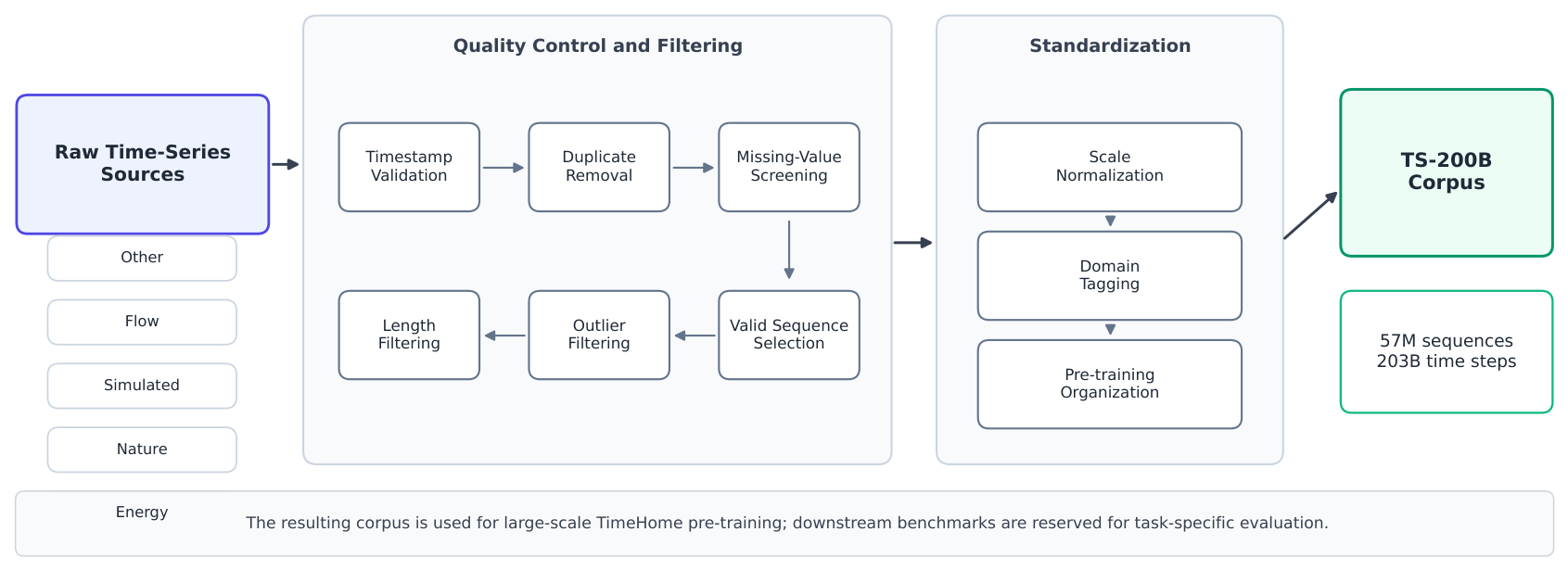
Data preprocessing and validation pipeline. To enhance the data quality and training stability, the raw records are processed by the preprocessing pipeline shown in
Figure 2. Firstly, the pipeline examines the timestamps and deletes the invalid, duplicated or inconsistent time records. Then, it eliminates the abnormal values, duplicate sequences, short sequences and records with many missing values. Subsequently, the remaining sequences are normalized to minimize the differences among various fields, are given domain labels and are compiled into the pre-training corpus. Thus, TS-200B contains different kinds of temporal data and avoids those which may cause instability in large-scale representation learning.
Dataset statistics and visualization. Table 3 presents the number of sequences and time steps in each TS-200B domain, and
Figure 3 depicts the domain distribution. The corpus includes temporal resolutions from sub-second measurements to annual summaries, supplying different degrees of details for TimeHome after processing. In contrast to small task-oriented datasets, TS-200B covers more varied time scales for joint pre-training on forecasting, imputation and anomaly detection.
2.8. Generative AI Use Declaration
During the preparation of this manuscript, the authors have employed ChatGPT-5.5, designed by OpenAI (San Francisco, CA, USA), merely for the purpose of language improvement, grammar correction and enhancing the clarity and readability of the manuscript. The system has not been utilized to produce research concepts, plan the study, collect data, draw figures, analyze results, interpret results or reach scientific conclusions. The AI-assisted parts have been thoroughly checked, revised and authenticated by the authors who are fully responsible for the content of the manuscript.
3. Results
3.1. Implementation Details
Training Configuration. Each model is trained for 100,000 steps with a batch size of 1024 and a maximum sequence length of 4096; thus, one iteration includes about 4 million time points. The output projection uses forecast horizons , and the auxiliary loss factor is kept constant at . Optimization uses Adam with lr = 1 × 10⁻³, weight_decay = 1 × 10⁻¹, , and . The learning rate follows a 10,000-step linear warmup and then cosine annealing. Training is conducted on 8 × NVIDIA A100-80G GPUs with bfloat16 (BF16) precision using Pytorch 2.0.
Technical Details. Our Heterogeneous Mixture-of-Experts (H-MoE) layer comprises a single shared expert alongside multiple independent experts, each implemented as a feedforward network (FFN) that is more lightweight than the conventional FFN used in dense models. The activation weight assigned to the shared expert for token t undergoes normalization via the Sigmoid function. In contrast, the activation weights corresponding to the i-th independent expert for token t are processed using the Softmax function. To enhance efficiency, we retain only the top-k highest-scoring independent experts while setting the remaining activation values to zero. The total number of experts is set to , with the top- experts activated per token. For the low-rank factorization in both expert and gating layers, the rank is set to .
3.2. Long-Term Time-Series Forecasting
Benchmark Details. We use eight datasets: Weather [
68], Traffic [
69], Electricity [
70], Exchange [
71], and the four Electricity Transformer Temperature (ETT) datasets (ETTh1, ETTh2, ETTm1, ETTm2) [
11]. The prediction windows are 96, 192, 336, and 720 time steps.
We also run a remote sensing extension experiment on GreenEarthNet. In this setting, the model predicts future vegetation dynamics from historical satellite-derived temporal signals. The experiment is intended to test whether the same backbone can handle remote sensing conditions such as cloud-contaminated observations, seasonal variation, and long-range temporal dependency.
Baseline Models and Metrics. The comparison includes baselines from several groups. ARIMA [
3] represents classical statistical forecasting, and LSTM [
40] represents recurrent neural forecasting. The foundation-model group includes TimesFM [
17], Chronos [
66], Lag-Llama [
16], Moirai [
51], and the MoE-based Time-MoE [
18]. We also keep recent forecasting baselines, including Peri-mid Former [
72], GPT4TS [
73], and TSLANet [
74]. The GreenEarthNet extension uses the same baseline set for consistency. Forecasting performance is measured by Mean Squared Error (MSE) and Mean Absolute Error (MAE).
Results. Table 4 reports averages over the four prediction lengths. TimeHome is strongest on ETTm1 (
MSE: 0.337, MAE: 0.362) and Weather (
MSE: 0.223, MAE: 0.262), and it also gives the lowest MSE on ETTm2 (
0.251). On Electricity and Traffic, the advantage appears mainly in MAE, with values of
0.221 and
0.266. Across all eight datasets, TimeHome has the lowest MAE (
0.332) and the second-lowest MSE (
0.314), so the improvement is not limited to a single dataset family.
The comparison is also informative by model type. ARIMA [
3] and LSTM [
40] lag behind on the averaged metrics, which is consistent with their weaker handling of long multivariate dependencies. Among foundation-style baselines, TimeHome has better performance than TimesFM [
17], Chronos [
66], Lag-Llama [
16] and Moirai [
51] in both average MSE and MAE. The difference in MSE between TimeHome and Time-MoE [
18] is small (0.315 to 0.314), while the difference in MAE is larger (0.338 to 0.332), indicating that the heterogeneous experts mainly decrease the absolute error rather than only modifying the squared-error behavior.
The probable reason is the division of work in H-MoE. Different measures are needed for continuous changes, abrupt fluctuations and localized irregularities, and the router can assign these token states to different expert procedures. Hybrid attention gives both local and distant contexts before routing, which reduces the chance that sudden changes are averaged. The auxiliary loss also improves the stability of the long-term optimization. These strategies suit the forecasting features, but more experiments are required to evaluate the separate impacts of each mechanism.
Remote Sensing Extension. GreenEarthNet provides a more direct remote sensing test.
Table 5 indicates that TimeHome has an MSE of 0.037 and an MAE of 0.132, which are both lower than those of the comparative methods. Compared with Time-MoE, the MSE decreases from 0.039 to 0.037, and the MAE decreases from 0.138 to 0.132. The result confirms the transfer from conventional time-series benchmarks to satellite-based vegetation forecasting, where cloud effects, seasonality and long-range dependencies occur simultaneously in the input data.
3.3. Time-Series Imputation
Benchmark Details. Imputation is judged based on the Weather and Electricity datasets and the four ETT datasets (ETTh1, ETTh2, ETTm1, ETTm2) [
11]. These datasets include various temporal patterns, forecasting horizons and input features.
Baseline Models and Metrics. We adopt the same baselines as in long-term forecasting in order to maintain consistency in the task comparison. The Mean Squared Error (MSE) and Mean Absolute Error (MAE) are used to evaluate the difference between the masked true values and the reconstructed values.
Results. Table 6 indicates that TimeHome has the minimum average MSE (
0.043) and MAE (
0.122) on the imputation benchmarks. The greatest improvements are observed on ETTm1 and ETTh1, where TimeHome achieves MSE values of
0.018 and
0.063. On ETTm2, Electricity and Weather, it is usually the second-best in individual metrics, but its overall average over the six datasets is still the lowest.
The result agrees with the model design. It is necessary to have both nearby context and longer temporal regularities for missing value recovery, which are provided by hybrid attention before the H-MoE routing. The masked expert is also relevant since it reduces part of the channel response, thus making the representation less influenced by unreliable local observations. Therefore, the improvement should be considered as the overall effect of reconstruction supervision, attention context and expert specialization, not from the performance of one module only.
3.4. Time-Series Anomaly Detection
Benchmark Details. Anomaly detection is evaluated by using five datasets: SMD [
75], MSL [
76], SMAP [
76], SWaT [
77] and PSM [
78]. Similarly to the TimesNet protocol [
12], all models use reconstruction error for the assessment.
Baseline Models and Metrics. The baselines are GPT4TS [
73], TimesNet [
12], PatchTST [
79], and Peri-mid Former [
72]. We indicate
F1-score,
Average Precision,
Recall and
Area Under ROC Curve (AUC).
Results. Table 7 indicates that the Average F1-score of TimeHome reaches 86.37%, which is close to GPT4TS and higher than the dense baselines. Its best result is the precision: the average precision is
88.42%, while it is 83.10% for TimesNet. The average AUC is
92.15%. This is important in anomaly detection since false alarms may have great influence on the cost of industrial monitoring. A plausible explanation is that masked experts reduce sensitivity to stochastic local noise, while the other experts preserve normal slow-varying patterns. Hybrid local–global attention further compares short deviations with a longer temporal baseline, which helps separate isolated measurement noise from sustained anomalous behavior.
3.5. Zero-Shot and Few-Shot Evaluation
Benchmark Details. To analyze the generalization capability of TimeHome in unseen domains and low-data environments, we conduct experiments on the Exchange dataset. The evaluation is performed under two distinct settings: Zero-Shot, where TimeHome is directly applied to the Exchange test set without fine-tuning, and Few-Shot, where the pre-trained model is fine-tuned using only 10% of the training data to simulate data-scarce industrial scenarios.
Baseline Models and Metrics. We compare TimeHome against two representative baselines: GPT4TS [
73] and TimesNet [
12]. MSE and MAE are adopted as the evaluation metrics.
Results. As shown in
Table 8, TimeHome performs well when little or no target-domain supervision is available. In the
Zero-Shot setting, it obtains an MSE of 0.435 and an MAE of 0.378, outperforming GPT4TS on both metrics. With only 10% of the training data in the
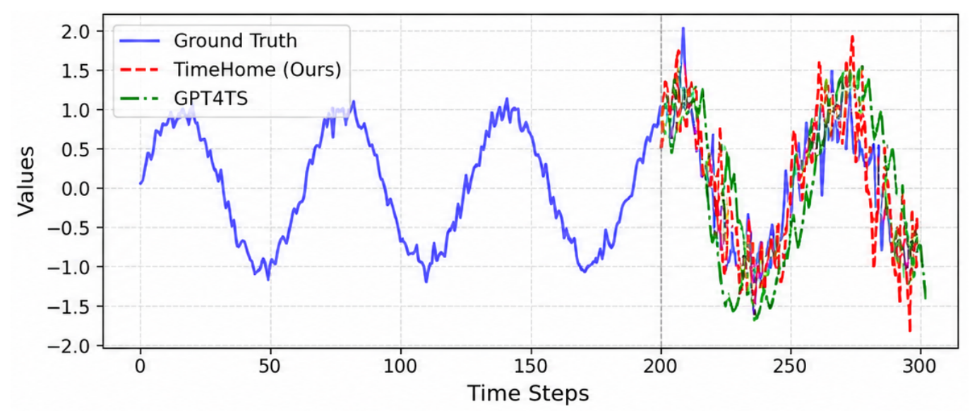
Few-Shot setting, TimeHome improves to an MSE of 0.405 and an MAE of 0.355, whereas TimesNet remains much higher in error.
Figure 4 gives a qualitative view of the same pattern: TimeHome follows the prediction trajectory more closely in the zero-shot horizon. These results suggest that the temporal patterns learned from TS-200B can be reused under limited supervision, rather than requiring the model to learn each target domain from scratch.
3.6. Ablation Studies
We use ablation experiments to separate the effects of the main TimeHome components.
Table 9 reports averaged task metrics across the datasets used in the main experiments. The efficiency metrics, including memory usage, FLOPs, and inference time, are measured on SWaT under the same hardware setting.
Removing the hybrid local–global attention lowers performance across all three tasks, which supports its role in multi-scale temporal modeling. The largest degradation occurs when H-MoE is removed: forecasting MSE increases from 0.314 to 0.342, imputation MSE increases from 0.043 to 0.056, and anomaly detection F1 decreases from 86.37% to 83.10%. Because the three tasks stress different behavior—trend prediction, missing-value recovery, and abrupt-change detection—this drop indicates that heterogeneous expert routing contributes beyond a single benchmark setting.
The ablation results also support the intended division of labor among the expert types. The zero expert is suited to stable or slowly varying structures, the masked expert to noisy or unreliable local observations, and the low-rank expert to non-trivial temporal changes. Replacing this structure with a standard dense MoE removes part of that functional specialization. The benefit of H-MoE therefore appears to come from the type of expert diversity, not only from the number of experts.
The efficiency ablations give a separate view of the design trade-off. Replacing low-rank matrices with full-rank matrices increases GPU memory from 7.2 GB to 13.5 GB and FLOPs from 4.1 G to 8.6 G, with little accuracy gain. Disabling Dynamic Expert Pruning raises FLOPs from 4.1 G to 6.9 G while leaving predictive performance nearly unchanged. These results support keeping both low-rank factorization and pruning in the final model.
3.7. Domain Sensitivity Analysis
In
Table 10, we compare forecasting performance across sectors to check whether the pre-training corpus creates an obvious domain bias. Energy has the largest time-step share, but it does not yield the lowest error. The Nature domain, with a smaller share than Energy, obtains the lowest average MSE of 0.233. This does not rule out all forms of domain imbalance, but it suggests that the observed performance is not explained simply by the volume of pre-training data in each sector. Signal predictability and the routing behavior of H-MoE are likely to be important as well.
3.8. Efficiency Analysis
We also benchmark computational efficiency against TimesNet [
12] and GPT4TS [
73].
Table 11 compares active parameters, FLOPs, and inference time.
Table 12 reports training time, peak memory, active parameters, FLOPs, and inference speed. TimeHome trains in 29.8 h, compared with 34.6 h for TimesNet and 61.3 h for GPT4TS. Peak memory is also lower at 38.4 GB/GPU, compared with 43.8 GB/GPU and 57.6 GB/GPU.
At inference time, TimeHome activates 14.2M parameters per step, fewer than TimesNet (42.5M) and GPT4TS (81.2M). Its FLOPs and inference time are 4.1G and 11.2 ms. These numbers match the intended role of low-rank factors and dynamic pruning: the model keeps a larger parameter pool available, but uses only a smaller active subset for each forward pass.
4. Discussion
The experiments suggest that TimeHome benefits from matching model capacity to the structure of the input sequence. Forecasting, imputation, and anomaly detection stress different parts of temporal modeling, yet removing H-MoE lowers performance across all three tasks. This supports the original design choice: stable intervals, noisy observations, and abrupt changes do not necessarily call for the same expert operation. The GreenEarthNet experiment also suggests that the design can transfer beyond standard public benchmarks, although the current remote sensing evaluation still covers a limited set of Earth observation conditions.
The results show a good equilibrium between the expressiveness and the cost. The low-rank decomposition and the dynamic expert pruning reduce the memory requirement, the number of Floating Point Operations (FLOPs) and the inference time. The ablation studies indicate a slight decrease in the performance of the target task. This is beneficial for saving long monitoring records, where an accurate but expensive model may not be feasible. Nevertheless, this equilibrium has its disadvantages. The low-rank factors restrict the parameter space, and if the variables are very complicated or appear infrequently, the compressed form might lose some information that a full-rank model can maintain.
There are still several limitations. First, the expert types in H-MoE are chosen empirically. The ablation study shows that they are useful, but it does not give a theoretical rule for choosing the best expert operations in a new domain. Second, TS-200B increases pretraining diversity, but it cannot cover every sensor, sampling protocol, or regional condition encountered in remote sensing practice. Third, the anomaly detection results focus on precision, while deployment may need different operating points if missed anomalies or false alarms are more costly.
We leave for future work the study of routing stability under domain shift, more adaptive pruning rules, and streaming or continual-learning settings where the temporal distribution changes over time.
5. Conclusions
This work presented TimeHome, a sparse transformer-based foundation model for unified time-series analysis. In this work, we used one backbone for forecasting, imputation, and anomaly detection. The purpose is to keep the model as practical as possible for noisy, incomplete, and heterogeneous temporal data.
TimeHome combines three elements: a functionally heterogeneous Mixture-of-Experts layer with dynamic expert pruning, tokenization with hybrid attention for multi-scale temporal dependencies, and TS-200B pretraining for broader temporal coverage. The experiments show competitive or improved performance in forecasting, imputation, anomaly detection, zero-shot and few-shot transfer, the remote sensing extension, and efficiency benchmarks. The ablations further indicate that H-MoE, low-rank factorization, and pruning each contribute to the final accuracy-cost trade-off.
The future work will be on routing stability under domain shift, adaptive pruning for resource-constrained deployment, and streaming or continual-learning scenarios in which the temporal distribution changes after deployment.