


Highlights
What are the main findings?
- A spatial-sequential 2DCNN-LSTM model was developed to retrieve submarine sand wave bathymetry from Sentinel-2 surface-reflectance textures.
- The model jointly captures local image textures and profile-scale rhythmic continuity of sand wave morphology.
- Independent multibeam validation shows that the model outperforms RF, CNN and LSTM baselines in the experiments.
What are the implications of the main findings?
- The proposed framework provides a low-cost approach for bathymetric mapping of sand wave fields where shipborne surveys are sparse.
- Model performance is strongly controlled by the visibility of sand wave-induced surface textures, highlighting the need for image-quality screening in operational applications.
Abstract
Submarine sand waves are widespread on shallow continental shelves. Their complex morphology and potential mobility create challenges for engineering surveys, navigation safety, and seabed stability assessment. Multibeam surveys provide accurate bathymetry but are costly and spatially limited, whereas satellite-based methods offer broader coverage but remain challenging in complex sand wave fields. Here, we propose a spatial-sequential 2DCNN–LSTM model for retrieving submarine sand wave bathymetry from Sentinel-2 surface reflectance imagery. The model represents each target point as a sequence of local multispectral image patches, allowing convolutional layers to extract two-dimensional textural features and LSTM layers to learn profile-scale rhythmic continuity associated with sand wave morphology. The model was trained using multibeam bathymetry and applied to a large extrapolation area of approximately 4000 km2 on the Taiwan Banks. Evaluation on the large extrapolated area against in situ bathymetric data achieved a root mean square error (RMSE) of 3.78 m, a mean absolute error (MAE) of 2.99 m, and a mean relative error (MRE) of 9.1%. The results demonstrate that sand wave-induced optical textures can provide useful information for broad-scale bathymetric reconstruction, although model performance remains dependent on image texture visibility controlled by hydrodynamic, illumination, and atmospheric conditions. This framework offers a cost-effective approach for satellite-based monitoring of large submarine sand wave fields, providing a new perspective for engineering applications.
1. Introduction
Submarine sand waves are rhythmic bedforms created by the interaction between marine hydrodynamics and sediments, extensively developed in continental shelf and shallow sea regions [1,2]. Their characteristic mobility poses significant threats to submarine engineering, the stability of shipping channels, and marine ecosystems [3]. Efficiently obtaining high-precision submarine sand wave topographic data is critical for accurately monitoring dynamic changes and engineering risks. Additionally, high-precision topographic data are important boundary conditions for reliable numerical modeling of hydrodynamics and geomorphic evolution [4]. At present, shipborne echo-sounder bathymetric survey remains the main means of acquiring precise submarine topography, but it has high costs and limited operational efficiency.
In recent years, with high-efficiency, low-cost, full-coverage remote sensing image data on seafloor topography, remote sensing-based bathymetric inversion has become a research focus. This approach leverages the response of underwater topography from observational data to achieve depth estimation through inverse reasoning. Currently, two primary methodologies are widely adopted: the radiative transfer equation [5,6] and hydrodynamic models [7]. The former relies mainly on the bottom reflectance component in remote sensing to invert water depth and is suitable for optically shallow waters [8]. The latter is based on the hydrodynamic-optical coupling mechanism. Underwater topography modulates near-surface currents, which in turn redistribute the slopes of micro-scale waves [9,10]. These slope variations create a pattern of alternating reflectance on the sea surface, translating into the characteristic light and dark stripes in satellite imagery that correspond to underwater topographic variations. It is primarily applicable to regions with rapidly changing topography and water depths ranging from approximately 10 to 70 m [11].
Synthetic aperture radar (SAR), an active microwave remote sensing system, offers advantages such as operational independence from solar illumination and the ability to penetrate cloud cover. SAR has become an important tool for detecting shallow-water and nearshore sand wave bathymetry [12,13,14,15]. The underlying detection mechanism involves the modulation of sea surface roughness and short-surface waves by sand wave topography [16]. For instance, the Bathymetry Assessment System developed by Calkoen et al. [17] based on SAR imagery is applicable in scenarios where sand wave orientation is perpendicular to the direction of tidal currents. Donato et al. [18] demonstrated that, even under weak wind and strong stratification conditions, SAR imagery can effectively identify sand wave topography with wavelengths of hundreds of meters. By integrating tidal current data, they successfully inverted sand wave bathymetry in shallow-water regions of the US continental shelf.
Compared with SAR, optical remote sensing offers higher resolution, richer spectral information, and broader data availability, and is unaffected by radar speckle noise, enabling improved identification of subtle topographic features [19,20,21]. Zhang et al. [22] retrieved local sand wave topography in the Taiwan Banks by mapping multiangle sun-glint images onto multibeam bathymetric data. However, this method is constrained by the image quality and the density of in situ measurements, resulting in limited extrapolation capability. Machine learning approaches have introduced new ideas for sand wave topography inversion by modeling nonlinear relationships between optical reflectance intensity and water depth [23,24,25,26,27,28,29]. Convolutional neural networks (CNNs) are capable of automatically extracting multilevel spectral and spatial features and have performed well in shallow bathymetric inversion [30,31,32]. Nevertheless, methods relying solely on CNNs to establish scale-dependent mapping patterns are influenced by training sample size and topographic complexity, making it difficult to effectively cope with highly variable underwater sand wave topography across extensive shoal areas. Furthermore, while multitemporal imagery can suppress random noise, it may also blur fine textural features within sand wave topography [33].
Recent studies have further emphasized three related issues in SDB applications: cross-domain generalization under varying water quality and atmospheric conditions, image-specific reliability limits of optical depth retrieval, and the potential of multi-source information to improve prediction stability under optically complex conditions [34,35,36].
Given that submarine sand waves exhibit notable spatial sequential characteristics owing to their undulating structures, sequence modeling methods such as recurrent neural networks (RNNs) have recently been introduced to the inversion of periodic and spatially continuous underwater topography. Among these, long short-term memory (LSTM) networks can effectively capture long-range dependencies and are suitable for modeling the continuous variation of sand wave profiles. By segmenting two-dimensional (2D) data into one-dimensional (1D) sequences along the profile direction, the spatial evolution patterns can be extracted in a manner analogous to time-series processing. Zhao et al. [37] transformed multisource remote sensing images into spatial sequences as input to an LSTM model for sand wave topography reconstruction in the Taiwan Banks. Leng et al. [9] applied an LSTM-based model to large-area bathymetric inversion in the Liaodong Shoal, China. The model was also applied in reef regions to reconstruct locally missing bathymetric signals, demonstrating the strong nonlinear modeling capability of LSTM in scenarios with missing optical signals or complex seabed environments [38]. To further incorporate bidirectional contextual information, bidirectional long short-term memory (BiLSTM) networks have been introduced. For instance, Xi et al. [39] proposed a Band-optimized BiLSTM model that uses an attention mechanism to identify sensitive spectral bands and achieve full-profile feature fusion. Zhu et al. [40] developed a hybrid CNN-BiLSTM model that combines the local feature extraction capability of CNNs with the sequence modeling ability of BiLSTM. The hybrid CNN-BiLSTM model performed well in clear waters but degraded in highly turbid environments. Some studies are not directly aimed at sand wave bathymetric inversion, but their hybrid approaches integrating convolutional feature extraction and recurrent sequence modeling offer valuable references for bathymetric inversion of sand waves [41,42].
Unlike conventional optical bathymetry in optically shallow waters, where depth information is mainly derived from bottom-reflectance attenuation, sand wave bathymetric mapping in the Taiwan Banks relies more strongly on surface texture patterns induced by the interaction between tidal currents, seabed topography, and illumination conditions. Therefore, the key challenge is not only spectral-depth regression, but also the extraction of spatial texture from multispectral imagery.
To address these limitations, this study proposes a spatial-sequential 2DCNN–LSTM framework for bathymetric mapping of submarine sand waves from Sentinel-2 surface-reflectance imagery. Instead of using single-pixel spectral values as sequential inputs, the proposed model constructs a sequence of local multispectral image patches along an approximately cross-crest direction determined from the dominant orientation of the major sand wave field. The main improvement of this framework lies in its sand wave-oriented spatial-sequential representation. Instead of treating the input as isolated pixels or simple one-dimensional spectral sequences, each target point is represented by a sequence of local multispectral image patches. This design allows the convolutional module to extract patch-scale optical texture associated with sand wave morphology, while the LSTM module learns the profile-scale rhythmic continuity of crest–trough variations. The objectives of this study are to: (1) develop a spatial-sequential deep learning framework for sand wave bathymetry retrieval; (2) evaluate its performance against RF, CNN, and LSTM baseline models using independent multibeam bathymetry; and (3) assess its large-area extrapolation ability and operational constraints over the Taiwan Banks.
2. Data Pre-Processing
The study area, Taiwan Banks, is located in the southern Taiwan Strait. With an average water depth of approximately 20 m and minimum water depths of less than 10 m [43], the Taiwan Banks extend 150 km from east to west and 80 km from north to south (Figure 1). This region features large-scale submarine sand wave fields [44]. The sand waves range between 5 and 20 m in height and from 300 to 2000 m in wavelength, exhibiting distinctive rhythmic, wave-like morphologies. Based on cross-sectional characteristics, the sand waves in this area can be categorized into double-crested and single-crested types, distributed in the western and eastern parts of the Banks, respectively [45]. Tidal waves from the East China Sea and South China Sea converge at the Taiwan Banks, creating a high-energy tidal current environment. It significantly enhances the modulation of sand wave topography on sea surface roughness. This allows the surface texture features induced by sand waves to be clearly identifiable in satellite imagery and offers distinct advantages for remote sensing-based inversion.
Figure 1.
Location of the Taiwan Banks. The black curve outlines the Taiwan Banks, and the solid box marks the bathymetric inversion area. An enlarged view of the solid box region is shown in Figure 2a.
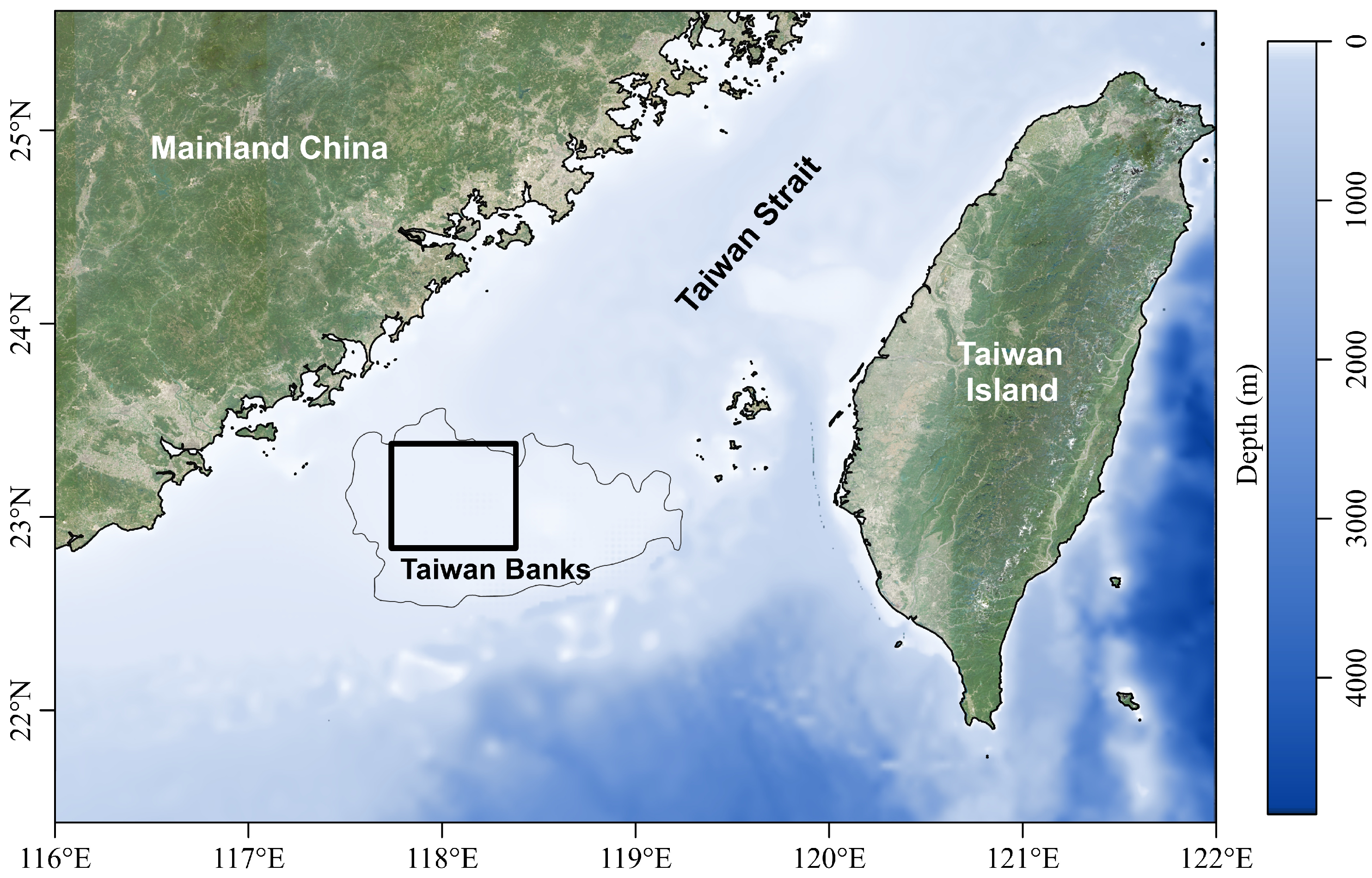
Figure 2.
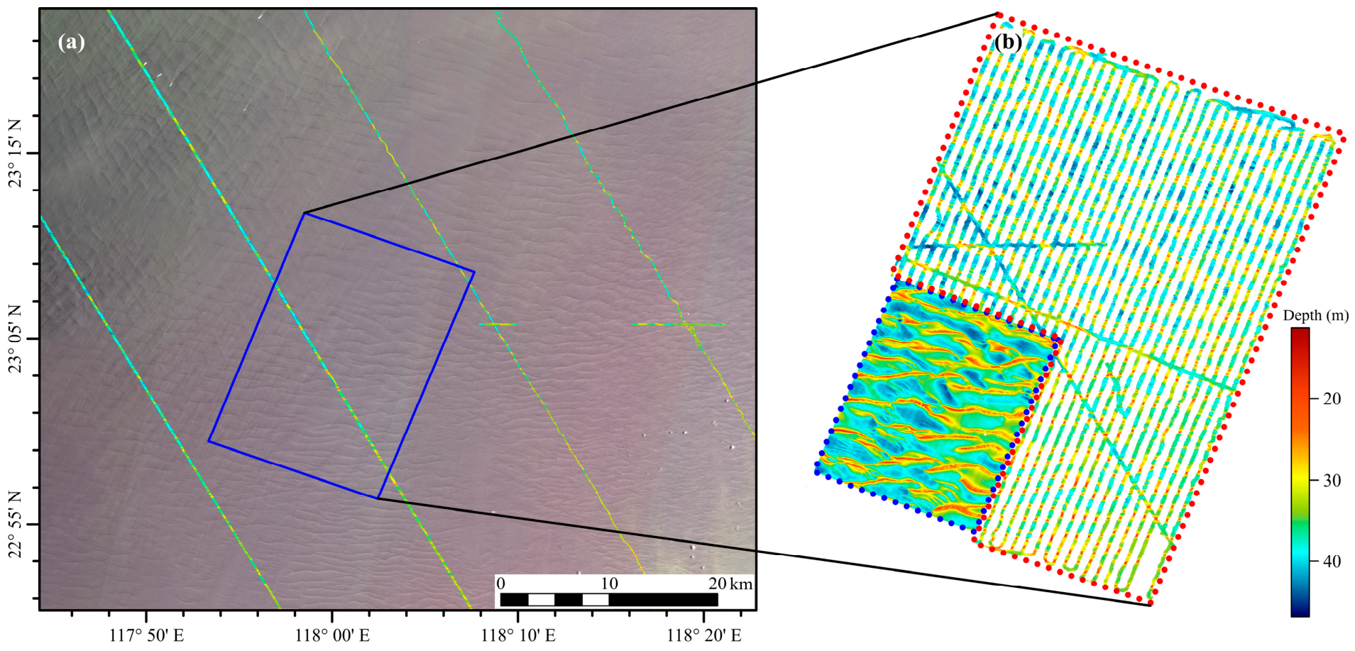
(a) Sentinel-2 image with multibeam swath data (collected in 2011) for accuracy evaluation. (b) The multibeam data used for the training (blue dotted area) and testing (red dotted area) datasets, which were collected in 2018 and 2012, respectively.
2.1. Sentinel-2 Data
Sentinel-2 is an Earth observation satellite of the European Space Agency’s Copernicus Programme and is equipped with a Multispectral Imager that provides 13 spectral bands at graded spatial resolutions of 10, 20, and 60 m. It serves as a key data source for global environmental and resource monitoring. The remote sensing dataset used for sand wave topography inversion in this study was derived from the Sentinel-2 Level-2A (L2A) surface reflectance product, publicly available via the official ESA data hub at https://browser.dataspace.copernicus.eu/ (accessed on 16 July 2024). The L2A product represents surface reflectance data that has undergone standardized pre-processing, including atmospheric correction, geometric rectification, and spectral response function calibration.
The image used was acquired on 7 July 2023, under cloud-free conditions over the study area. Using the remote sensing data processing software ENVI 5.6, the L2A reflectance image was subjected to band selection (B2, B3, B4), mosaicking, and cropping. The digital number (DN) values were then converted to surface reflectance values, and the image was clipped according to the geographic extent of the study area. The resulting image used for bathymetric inversion covers an area of approximately 4000 km2, measuring 60 km in north–south extent and 66 km in east–west extent, with a spatial resolution of 10 m (Figure 2a).
The Taiwan Strait is strongly influenced by the East Asian monsoon, with a strong northeast monsoon in winter and a weaker southwest monsoon in summer [46], which can affect regional wind, sea-state, and surface-roughness conditions. The Taiwan Banks are also characterized by strong tidal currents and large sand wave fields, providing favorable conditions for surface-texture imaging of seabed topography under suitable environmental and illumination conditions. During image screening in this study, warm-season Sentinel-2 scenes more often showed clear and continuous sand wave textures, whereas many winter scenes were affected by weak or discontinuous texture, cloud contamination, or rough sea-state conditions. Therefore, the main inversion image was selected from a cloud-free warm-season Sentinel-2 scene acquired on 7 July 2023. Additional Sentinel-2 scenes acquired on 8 June 2019, 28 May 2021, and 22 June 2023 were used for cross-date applicability assessment in Section 4.3.
2.2. Multibeam Bathymetric Data
The multibeam swath data used in this study were collected in 2011 (Figure 2a) and 2012 (Figure 2b), covering a total area of approximately 160 km2. These datasets were used for error assessment of the bathymetric inversions in both the test and extrapolation areas. The data collected in 2018 (Figure 2b) provided full multibeam coverage over an area of approximately 76 km2 and were used to construct water depth labels for the training and validation sets (Table 1).
Table 1.
Summary of the measured bathymetric data.
The multibeam systems included the R2 SONIC 2024 (R2Sonic, LLC, Austin, TX, USA) and Teledyne RESON SeaBat 7125 SV2 (Teledyne RESON A/S, Slangerup, Denmark), operating at a frequency of 400 kHz with up to 512 beams. The relative depth measurement error was lower than 1% of water depth. Positioning was achieved using a NavCom SF-3050 system (NavCom Technology, Inc., Torrance, CA, USA) integrated with StarFire/RTK GNSS, providing a positional accuracy of approximately ±0.15 m [44]. The raw multibeam bathymetric data were processed using Caris HIPS & SIPS 8.1. The processing steps included position and attitude correction, draft-tide-sound velocity compensation, outlier filtering, and data fusion. Finally, a 10 m resolution digital bathymetric model was generated to match the spatial resolution of the Sentinel-2 L2A imagery.
It is important to note that the training and validation datasets used in this study were acquired during different survey periods. In our previous work, we investigated the dynamics of sand waves on the Taiwan Banks, where giant sand waves constitute the dominant sand bodies. High-resolution multibeam bathymetric data collected over a three-year interval were used to examine their morphological evolution. The results demonstrated that these giant sand waves—which serve as the target features for bathymetric inversion in the present study—exhibit negligible migration at annual time scales [47]. Moreover, these giant sand waves are widely regarded as relic bedforms. Therefore, although the satellite imagery and in situ bathymetric data were not acquired contemporaneously, the morphology of giant sand waves serving as the basis for model training and validation is expected to have remained broadly stable over the time span considered. In other words, the temporal mismatch does not fundamentally compromise the rationality of the data combination in this specific study area.
3. Methods
3.1. 2DCNN-LSTM Framework
To enhance the spatial representation of sand wave topography in sequence-based inversion models, this study proposed a deep learning-based bathymetric inversion model that integrated a CNN and a LSTM network. This end-to-end paradigm directly maps input Sentinel-2 L2A multispectral remote sensing images to water depth values at target points (Figure 3a). The model consisted of two components: a convolutional module for extracting spatial bathymetric features and a sequential module for capturing spatial sequence variations in water depth, each designed with specific purposes. Unlike existing LSTM models that rely solely on pixel-based sequences, the proposed model leveraged the strengths of CNN in extracting spatial features. It captured the response of micro-scale surface waves to undulating submarine topography within a spatial window, effectively expanding the receptive field from point-scale to patch-scale. This allowed the model to incorporate broader contextual information, enabling a more comprehensive perception of underwater topographic variations. Building on the spatially represented bathymetric features, the LSTM modeled the rhythmic variation patterns of sand wave topography, ultimately producing inverted water depths based on sequential dependencies.
Figure 3.
(a) Architecture of the bathymetric inversion using the 2DCNN-LSTM model, (b) structure of the LSTM, and (c) LSTM block.
The training dataset in this study came from spatially co-registered Sentinel-2 surface reflectance imagery and multibeam bathymetric raster data, where the former served as input and the latter provided ground truth labels. To evaluate the model’s inversion performance, the trained model was directly deployed over a larger experimental area to extrapolate the bathymetric inversion of extensive sand wave terrains. The accuracy and robustness of the model were assessed using multibeam swath data. Overall, the 2DCNN-LSTM model operates without relying on any prior background constraints, and its end-to-end paradigm allows direct prediction of water depth from the input Sentinel-2 L2A surface reflectance data.
The framework differs from conventional CNN-LSTM hybrids mainly in the way the input sequence is constructed for sand wave bathymetry. In many hybrid CNN-LSTM models, convolutional features are extracted from consecutive images, temporal frames, or generic spatial samples before being passed to a recurrent module. In this study, however, the sequence is not a temporal sequence, but a sand wave-oriented spatial sequence. Each sequence step corresponds to a local multispectral image patch centered on a point along the predefined profile direction. Therefore, the LSTM does not operate on single-pixel spectral values, but on patch-scale texture representations extracted by the 2DCNN module. This design enables the model to jointly represent local two-dimensional optical texture and profile-scale crest–trough continuity, both of which are important for retrieving submarine sand wave bathymetry from Sentinel-2 imagery.
3.1.1. Convolutional Spatial Bathymetric Feature Extraction Module
CNNs offer distinct advantages in processing raster imagery by automatically capturing nonlinear relationships between a central pixel and its surrounding pixels, thereby eliminating the need for handcrafted feature design. A core component of the CNN is the convolutional layer, which leverages the local receptive field mechanism to extract spatial dependencies among pixels—each neuron connects only to a localized region of the input image. Sand wave topography exhibits ripple-like morphological characteristics at spatial scales. Traditional methods often treat each pixel in isolation, reflecting only the water depth response at that specific location. In contrast, the CNN used convolutional kernels that slid across local windows, simultaneously capturing information from both the central pixel and its surrounding neighborhood. This enabled the model to perceive the spatial morphology and structure of sand waves. Through this mechanism, the model could identify both overall trends and local variations in underwater topography, rather than merely estimating depth values at individual points.
The multibeam-measured water depth points were used as prior labels. For each point, an image patch of size W × H × C (Width × Height × Bands) was extracted from the Sentinel-2 L2A imagery, centered at the corresponding location. Previous studies have indicated that deeper network architectures are often unsuitable for underwater topography inversion owing to limited data availability and relatively simple structures [30,48]. Therefore, in the convolutional module adopted in this study, we designed a hierarchical yet concise 2D convolutional structure specifically for extracting spatial features from multispectral remote sensing image patches. The module consists of three sequential convolutional layers. The first two layers use 3 × 3 convolutional kernels with 16 channels, focusing on capturing local spatial features. The third layer increases the channels to 32 to extract more complex spatial patterns. A non-overlapping max-pooling layer with a 2 × 2 kernel was inserted after the second convolutional block, performing down-sampling in the spatial dimensions. This operation expands the receptive field, enabling the model to perceive larger-scale sand wave topographic features. It also enhances the spatial invariance of the features and helps mitigate overfitting. All convolutional layers used the ReLU activation function, which strengthened the model’s capability for nonlinear fitting while effectively alleviating issues such as vanishing gradients and overfitting.
After processing by the 2DCNN module, the original image patches were transformed into a set of highly condensed feature maps. These intermediate features essentially encoded the characteristics of underwater topographic variations at spatial scales within the remote sensing imagery. As a result, each element in the subsequently generated sliding-window sequences no longer represented point-scale water-depth response features from a single pixel in the original image, but rather incorporated patch-scale features that included spatial contextual information from a certain surrounding area. This enriched patch-scale representation and provided a more informative input basis for the subsequent LSTM module to analyze dynamic changes in features along the sequence dimension.
3.1.2. Sequential Water Depth Variation Feature Extraction Module
Sand wave topography exhibits not only distinct spatial ripple-like patterns but also ordered and periodic variations along the sequential dimension. These continuous variation characteristics share a high similarity with time series, requiring models capable of capturing long-range dependencies for effective representation. As an improved variant of RNNs, LSTM networks introduce memory cells to transmit information across sequence steps, thereby successfully mitigating the gradient explosion and vanishing gradient problems commonly encountered in traditional RNNs when processing long sequences. As such, LSTM is particularly well suited for predicting continuously varying topographic features.
Within the 2DCNN-LSTM architecture, the LSTM undertook the core function of sequence modeling. The high-level spatial feature tensor extracted by the 2DCNN module was flattened into a 1D vector. Each vector represented a patch-scale feature at the corresponding water depth point and was enriched with spatial contextual information. By modeling these sequentially arranged feature sequences, the LSTM adaptively learned the trend variation patterns of sand wave topography in the spatial domain, and ultimately achieved accurate mapping from spatially sequential features to water depth values.
Before constructing the spatial-sequential samples, the Sentinel-2 image and the corresponding bathymetric grid were rotated according to the dominant orientation of the major sand wave field. This preprocessing step was used to make the sequence direction approximately aligned with the cross-crest direction of the dominant giant sand waves. For each target pixel, a sequence of neighbouring image patches was then extracted along this approximately cross-crest direction and used as the input to the LSTM module.
It should be noted that this procedure represents a dominant-orientation approximation rather than a locally adaptive estimation of the crest-normal direction for every individual sand wave. This design was adopted because the Taiwan Banks contain a large-scale sand wave field with a generally coherent dominant orientation, whereas local crest orientations may still vary in areas with curved, bifurcated, or superimposed bedforms. Therefore, the extracted sequences are expected to capture the main crest–trough spatial dependency of the dominant sand waves, while local orientation variability is treated as part of the natural morphological complexity of the study area.
Specifically, based on the output from the 2DCNN module, the input sequence for the LSTM was constructed using 1D feature vectors with a sequence length of L steps and a data dimension of L × 32 (Sequence × Neurons). We designed a three-layer LSTM structure with 32, 64, and 128 neurons in each layer, respectively, and used the ReLU activation function. This design enabled the model to fully leverage the sequential contextual information underlying the variation in sand wave topography.
The LSTM could adaptively learn the variation patterns of sand wave topography in the spatial domain and identify characteristic trends through its unique gating mechanism (see Figure 3b,c for the structure). The LSTM unit incorporated an input gate, a forget gate, and an output gate to selectively forget or retain information. The internal information transfer process within the LSTM unit can be described by the following equations:
where , , and denote the forget gate, input gate, and output gate, respectively, representing the proportion of the signal allowed to pass, with values in the range [0, 1]. denotes the 1D input vector at the step of the water depth sequence. is the output of the tanh function at step , indicating the current cell state, which ranges between [−1, 1]. represents the output of the LSTM unit at step , and denotes the output from the previous LSTM unit. and (with subscripts , , and ) refer to the weight vectors and biases of the gates under different states. Through this gating mechanism, the long-term memory retained in and the short-term memory carried by were passed to the next LSTM unit.
After sequential modeling by the LSTM, all features were transformed into a 1D output vector (Figure 3b), which was subsequently passed through a fully connected (Dense) layer to produce the final water depth prediction. By deeply mining the variation patterns of sand wave topography embedded in the sequences, the LSTM module converted the dynamic evolution of spatial features within the spatial domain into an accurate inversion of water depth at the target point, ultimately outputting the predicted depth value.
3.2. Baseline Models
To ensure a fair and reproducible comparison, we systematically evaluate the proposed model against three comparative models: a Random Forest (RF), a CNN, and a LSTM. All models are designed to address the same predictive task. The input data for each model is structured to match its architectural strengths: sequential data for LSTM, spatial data for CNN, and spatial-sequential data for the proposed model, all derived from the same source. Crucially, the key dimensions (e.g., sequential size, spatial size) are made comparable across models where applicable. The core architectural designs are summarized in Table 2 to facilitate a direct comparison.
Table 2.
Summary of comparative model architectures and parameters.
3.3. Model Training Strategy
Following the construction of the 2DCNN-LSTM model architecture, a stochastic gradient descent-based optimization algorithm was employed to train the model parameters. The model input was constructed by extracting pixel sequences of length 20 along the approximately cross-crest direction determined from the dominant orientation of the major sand wave field. For each point in the sequence, a 9 × 9 image patch centered on that point was extracted from the blue, green, and red bands, forming a tensor with dimensions of 20 × 9 × 9 × 3 as the input dataset for the model. Given the 10 m spatial resolution of Sentinel-2, the 9 × 9 patch corresponds to a local window of approximately 90 m × 90 m, while the sequence length of 20 provides an approximately 200 m spatial context along the predefined sequence direction. The basis for selecting these input dimensions is further discussed in Section 5.1.2.
The input dataset was divided into a training set (80%) and a validation set (20%), with the training data shuffled at the beginning of each epoch to enhance the model’s generalizability. The Adam optimizer was selected for model training owing to its adaptive learning rate adjustment mechanism, which is well-suited for efficiently optimizing the numerous parameters in the 2DCNN-LSTM architecture.
Regarding the initial learning rate, we chose 1 × 10⁻⁴ based on a balance between model depth and data characteristics. Our 2DCNN-LSTM, being a deep network, requires stable updates to avoid divergence. More importantly, as our dataset was constructed by extracting image patches, it inherently contained sample noise. A smaller initial learning rate was chosen to prevent the model from overfitting to such noise within early batches, thereby encouraging more robust feature learning and better generalizability. To further refine the training process, a dynamic learning rate scheduling strategy (ReduceLROnPlateau) was introduced. If the validation loss failed to decrease for four consecutive epochs, the learning rate was reduced to 50% of its current value, with a lower bound set at 1 × 10⁻⁶. This strategy effectively mitigated training plateaus: after each learning rate reduction, the validation loss resumed a stable downward trend, leading to smoother convergence and preventing abrupt fluctuations in the late training stages.
All hyperparameters were selected considering the model’s complexity and dataset properties. For batch size, we selected 128 as an optimal compromise. While a smaller batch size (e.g., 32) could lead to high gradient variance and unstable training, a larger batch size improves training stability but increases memory demand. The total number of training epochs was set to 100, as empirical observations confirmed that the model reliably converged within this span. To prevent overfitting, an early stopping mechanism was applied, monitoring the validation loss with a patience of 8 epochs and mode set to "min". The model checkpoint with the lowest validation loss was saved for final evaluation. This early stopping criterion not only prevented overfitting but also reduced training time compared to fixed-epoch training.
3.4. Model Evaluation Metrics
We quantitatively evaluated the accuracy of the inverted water depths using RMSE, MAE, MRE, and the coefficient of determination (R2), and systematically analyzed the inversion performance. Among these metrics, RMSE—calculated by squaring, averaging, and then taking the square root of errors—is more sensitive to large errors and effectively reflects the overall deviation of the inverted water depth values. MAE measures the average absolute difference between the inverted and measured values, providing a robust representation of the general error magnitude. MRE expresses errors in relative terms, which eliminates the influence of absolute units and facilitates comparisons across different regions or scales of water depth data. Lower values of these three metrics indicated higher inversion accuracy and better model stability. R2 was used to evaluate the model’s ability to explain the variance in water depth variations; a value closer to 1 indicated a better fit between the inverted results and the measured values, reflecting the superior predictive performance of the model.
where = 1, 2, 3, …, n, n is the number of bathymetric points used to validate the models, is the bathymetric value, and is the predicted depth value.
4. Results
To evaluate the accuracy of the trained model, two extrapolation experiments at different scales were conducted in the shoal area. For the small-scale test region (as shown in Figure 2b), the multibeam swath data acquired in 2012 were used to assess the accuracy of the inverted topography, with comparisons made against RF, CNN and LSTM models. For the large-scale extrapolation area (as shown in Figure 2a), the inversion results were evaluated using multibeam swath data collected in 2011.
4.1. Testing Area Results
The images were input into the 2DCNN-LSTM and three comparative models to obtain the bathymetric inversion results of the sand wave topography. Statistical analysis based on 9701 spatially aligned predicted-measured data pairs (Figure 4) showed that in terms of overall inversion performance, the bathymetric inversion results of all four models exhibited significant clustering along the 1:1 reference line, with the highest point density observed in the 30–40 m water depth interval, consistent with the main developmental depth of sand waves in this region. In shallow water areas (<25 m), however, owing to the influence of sharp-peaked sand wave morphology (mean wave height > 10 m) on the Taiwan Banks, topographic complexity increased significantly. The uneven distribution of measured points across different water depths resulted in relatively low sampling density at the sand wave crests.
Figure 4.
Scatter density plots of water depth predicted by four models and the actual measured water depth. The dashed line indicates the 1:1 reference line.
In terms of the performance of different model architectures, the RF model’s error distribution is the most dispersed, with RMSE and MAE values of 4.64 m and 3.73 m, respectively. By integrating spatial contextual information from neighboring regions, the CNN model optimized the RMSE to 4.38 m, reducing it by 6% compared with the RF model. This indicated that predicting rhythmic sand wave topography requires adequate consideration of its variation characteristics across spatial scales. The LSTM model achieved further improved accuracy compared to the CNN model, demonstrating its predictive advantage in rhythmic sand wave topography. By leveraging its ability to jointly perceive spatial features and sequential variations, the 2DCNN-LSTM model achieved the best convergence performance, demonstrating a marked improvement in accuracy over the baseline models. This validated the effectiveness of incorporating spatial features and rhythmic variation constraints in improving the accuracy of sand wave topographic inversion.
Figure 5a–d displays the predicted water depth maps of the sand wave field generated by the four models: RF, CNN, LSTM and 2DCNN-LSTM. Overall, the water depths predicted by each model exhibited certain similarities at the macroscopic scale, with major sand wave crest lines effectively captured in all cases. Due to the point-to-point water depth prediction approach of the RF model, the resulting map (Figure 5a) exhibited numerous scattered noise points that lacked a discernible directional pattern in the distribution. Figure 5b showed that the CNN model yielded predictions with better overall spatial continuity; its convolutional architecture effectively extracted the neighborhood features of the sand wave topography, though some block-like noise remained. In Figure 5c, the LSTM result showed relatively good continuity along the predefined sequence direction, but weaker spatial continuity in the transverse direction. This is because the LSTM baseline operates through one-dimensional sequential prediction and therefore tends to produce directionally biased spatial patterns. In contrast, the 2DCNN-LSTM model demonstrated more continuous and smoother spatial characteristics by combining patch-scale spatial feature extraction with sequential dependency modeling.
Figure 5.
(a–d) represent the bathymetric maps of sand waves for the four models. The black solid line indicates the profile position, which was used to display the profile comparison results.
Figure 6 presents a profile comparison between the water depths predicted by the four models and the measured values, while Table 3 provides the corresponding error evaluation metrics. In Figure 6a, the RF model performed poorly in predicting extreme points, resulting in a significant underestimation of sand wave height. In Figure 6b, the prediction results of the CNN model showed significantly reduced noise, appearing smoother and more continuous overall, with a good fit to the measured values. This indicated that incorporating spatial neighborhood information enabled a more accurate capture of the directional variation features of sand waves. Nevertheless, in certain complex areas (e.g., within the X-axis range of 12,000–17,000 m), noticeable discrepancies remained between the predicted and measured values. Two adjacent sand waves were not predicted accurately (blue boxes in Figure 6a,b), reflecting the model’s limited ability to capture rapid local changes in water depth. Further improvements were needed to enhance accuracy in inverting complex topography. Although the LSTM model effectively captured the variation trend of sand waves, some noise persisted, stemming primarily from the mismatch between the sequence prediction direction and the profile direction (Figure 6c). This indicated that using only sequential models had inherent directional limitations in feature extraction.
Figure 6.
The profile comparison of predicted water depth and measured water depth of the four models. The blue solid line represents the measured water depth, and the red solid line represents the predicted water depth. The blue solid boxes in (a,b) indicate typical areas where the sand waves were not accurately predicted.
Table 3.
Error evaluation metrics along the representative testing profile shown in Figure 6.
In comparison, the 2DCNN-LSTM model demonstrated the best performance, with its predicted curve closely aligned to the measured values across most intervals, maintaining high consistency even in regions with significant depth variations. As shown in Table 3, this model achieved RMSE, MAE, and R2 values of 3.45 m, 2.68 m, and 0.64, respectively, significantly outperforming the other models in all metrics. These results indicated its stronger adaptability and inversion accuracy in complex data environments.
Overall, all four models had some capabilities in bathymetric inversion. The RF model significantly underestimated sand wave height and exhibited substantial noise in its predictions. The CNN model showed better smoothness and spatial continuity, although its accuracy in locally complex topography still required improvement. LSTM could stably capture the overall trends of sand waves but suffered from directional limitations and noise interference. By integrating spatial features and sequence rhythmic information, the 2DCNN-LSTM model achieved more precise water depth predictions in most scenarios, demonstrating superior comprehensive performance and applicability.
4.2. Extrapolation Area Results
The results from the test area demonstrated that the 2DCNN-LSTM model combined with Sentinel-2 L2A imagery could achieve more accurate water depth predictions. This study extended the application of the model to a large-scale area over the Taiwan Banks. Figure 7 presents the resulting inverted sand wave topography map, in which four bathymetric swath datasets from the eastern to western regions serve as measured ground truth for a systematic evaluation of the model’s prediction performance. Figure 8 shows the scatter density distribution between the model-predicted water depths and the measured depths from the four swaths, with corresponding error metrics provided in Table 4.
Figure 7.
The bathymetric map of the study area on the Taiwan Banks, with black swaths representing multi-beam data.
Figure 8.
Scatter density plots of predicted water depth and measured water depth for (a) Profile 1, (b) Profile 2, (c) Profile 3, (d) Profile 4, and (e) all four profiles combined. The dashed line indicates the 1:1 reference line.
Table 4.
Evaluation of the error between predicted water depth and measured water depth.
As observed in Figure 7, the model successfully identified the overall morphology of large sand waves, with macro-features such as crest positions and orientations clearly discernible. Across the entire study area, sand waves were predominantly concentrated in the central region, while the edges were relatively sparse. In the northwestern part, sand wave distribution is scattered with wide intervals. The model tends to generate false topographic undulations in these flat zones, indicating that its sequential pattern extraction mechanism may over-interpret weak reflectance variations as topographic signals when sand wave density is low. The southeastern region exhibited dense sand wave coverage where multiscale sand wave superposition led to higher topographic complexity, increasing prediction difficulty. The model tends to produce over-smoothed results, which leads to a systematic underestimation of peak values and a loss of high-frequency topographic detail in these extrapolation zones. The central area showed relatively uniform sand wave distribution, gentler topography in trough regions, and less interference from noise, resulting in higher prediction quality. The main local artifacts were observed in two types of areas. In sparsely developed sand wave areas, the model occasionally generated weak sand wave-like undulations that were not clearly expressed in the multibeam bathymetry. In densely developed or superimposed sand wave areas, the predicted bathymetry tended to be smoother than the reference bathymetry, with reduced crest–trough amplitudes and weakened small-scale relief. These artifacts indicate that the model performs better in areas where rhythmic sand wave texture is clearly expressed, whereas prediction uncertainty increases in areas with weak, discontinuous, or multi-scale texture patterns.
Figure 8a–d presents scatter density distributions of predicted values from the 2DCNN-LSTM model against in situ measurements along four transects from east to west, with all comparisons based on 31,033 spatially matched data points. Overall statistical results (Figure 8e) showed that the scatter points exhibited clear clustering along the 1:1 line, indicating good overall agreement between predictions and measurements, although certain prediction deviations were observed within the 40–50 m water depth interval. The entire study area displayed a sand wave distribution pattern that was sparser in the north and denser in the south, and this spatial heterogeneity was accurately captured in the predictions. The model successfully identified the crest positions of all significant sand wave features and effectively represented water depth variations from crest to trough.
The error metrics in Table 4 show that the overall RMSE, MAE, MRE and R2 for the entire region were 3.78 m, 2.99 m, 9.1% and 0.42, respectively. Among these, Profile 2 achieved the best performance across all metrics (RMSE = 2.79 m, MAE = 2.18 m, MRE = 6.3%, R2 = 0.52). This is not only due to its proximity to the training dataset location, but more importantly because the sand waves in this profile are regularly spaced with relatively uniform morphology, and the depth range (predominantly 25–35 m) closely matches that of the training set (mainly 30–40 m). In contrast, Profile 3, located in the southeastern area where multi-scale sand wave superposition increases topographic complexity, yields the highest RMSE (4.26 m).
In summary, the 2DCNN-LSTM model could accurately represent most large sand wave topography when the spatial distribution of sand waves was relatively uniform. However, in areas where sand waves were sparsely distributed or exhibited complex morphologies, the model remained susceptible to noise interference, leading to artificial topographic features, although it could still capture the overall variation trends. The interaction between unseen topographic complexity and non-uniform data distribution primarily constrains accuracy in extrapolation regions.
These errors may arise from residual noise signals in the remote sensing imagery that have not been fully eliminated, as well as insufficient diversity of sand wave morphologies in the training dataset. Future efforts could focus on enhancing noise filtering and expanding the coverage of training samples to further improve the prediction accuracy and robustness of the model under complex conditions.
4.3. Cross-Date Applicability
To assess the cross-date applicability of the model, the trained model (using the 7 July 2023 image) was applied to images of the testing area acquired on different dates. Figure 9a–c shows images acquired on 8 June 2019, 28 May 2021, and 22 June 2023, respectively. The overall image texture is clear, with cloud coverage present in Figure 9b,c, though the cloud-covered area accounts for a minimal proportion.
Figure 9.
Images acquired (a–c) on three different dates (8 June 2019, 28 May 2021 and 22 June 2023), and corresponding bathymetric inversions (d–f).
As shown in Figure 9d–f, which present the predicted bathymetry for the three dates, a summary of the quantitative accuracy is provided in Table 5. The analysis indicates that the accuracy of the predicted bathymetry exhibits varying degrees of decline. Because the physical mechanism of sand wave imaging relies on the modulation of surface roughness by the interaction between tidal currents and topography, the images acquired on different dates record different weather conditions. From the predicted bathymetry maps for 2019 (Figure 9d) and 2023 (Figure 9f), it can be observed that the spatial distribution of sand waves is similar. However, some individual sand waves were not accurately predicted, corresponding to areas with very weak texture in the original images. In contrast, the predicted bathymetry for 2021 (Figure 9e) shows improved accuracy, characterized by clearer, more complete sand wave crests and enhanced detail in the trough areas. However, it also contains some noise introduced by the image.
Table 5.
Cross-date validation accuracy and compact scene-quality indicators for Sentinel-2 images over the testing area.
The cross-date applicability demonstrated by the 2DCNN-LSTM fundamentally stems from the model’s ability to extract and model features of complex spatial relationships and textural information. However, it should also be noted that the model relies heavily on the richness of textural information in the images, which provides guidance for image selection.
To examine whether cross-date performance was related to scene quality, several compact image-derived indicators were added to the validation results. Cloud pixels, sun zenith angle, and mean visible reflectance from B2–B4 were used to describe cloud contamination, illumination condition, and visible-band water optical background, respectively. These indicators provide a concise description of the selected Sentinel-2 scenes and help explain the differences in cross-date validation performance.
As shown in Table 5, the four scenes had similar solar illumination conditions, with sun zenith angles ranging from 17.22° to 18.78°. In contrast, mean visible reflectance showed a clearer correspondence with validation error. The image acquired on 7 July 2023 had the lowest mean visible reflectance and achieved the best accuracy, whereas the 8 June 2019 and 22 June 2023 images had higher mean visible reflectance and larger RMSE values. This suggests that a brighter visible-band water background, possibly related to water-color variability, turbidity-related reflectance, residual glint, or surface-reflectance effects, may weaken the stability of sand wave-related texture used by the model. These indicators should therefore be interpreted as practical scene-quality descriptors for the selected images.
5. Discussion
5.1. Ablation Experiments and Analysis of Key Parameters
To validate and optimize the key input parameters of the model, we conducted systematic ablation experiments focusing on the spectral band combinations of the imagery, the spatial size of image patches, and the spatial sequence length. The physical foundation of our method lies in utilizing the spatial texture (or roughness) patterns induced by sand wave topography to invert water depth, rather than relying on the direct radiative transfer. Therefore, parameter selection aims to optimally capture texture information correlated with depth while suppressing irrelevant noise.
5.1.1. Sensitivity Analysis of Spectral Band Combinations
We tested four different Sentinel-2 band combinations to evaluate their impact on bathymetric inversion accuracy (Table 6). All combinations were tested under identical configurations.
Table 6.
Bathymetric inversion performance of different band combinations on the testing set.
The experimental results indicate that using only the three visible bands—blue (B2), green (B3), and red (B4)—achieved the best inversion accuracy (R2 = 0.47, RMSE = 3.72 m). Within the framework of this study’s texture-based sand wave bathymetric inversion, the B2, B3, and B4 bands of Sentinel-2 constitute an optimal combination that maximizes the capture of topography-related texture signals while minimizing interference from irrelevant noise.
It is worth noting that the performance differences among the four band combinations are relatively small (Table 6): the RMSE values range from 3.72 m to 3.89 m, and the MRE values range from 8.8% to 9.2%. This suggests that the choice of spectral bands does not lead to dramatic variations in inversion accuracy. In practical applications, the selection of band combinations may therefore be determined empirically based on the actual model performance, considering factors such as data availability, computational efficiency, or specific local water conditions.
5.1.2. Optimization of Spatial Texture and Sequence Length
The size of the image patch determines the local spatial texture pattern that the model can perceive. This is particularly important for sand wave bathymetric inversion because the model relies on sand wave-induced optical texture rather than direct bottom reflectance. Since the Sentinel-2 bands used in this study have a spatial resolution of 10 m, the tested patch sizes of 3 × 3, 5 × 5, 7 × 7, 9 × 9, and 11 × 11 correspond to approximate ground windows of 30 m × 30 m, 50 m × 50 m, 70 m × 70 m, 90 m × 90 m, and 110 m × 110 m, respectively. We first fixed the sequence length at 30 and tested the performance of different image patch sizes (Table 7).
Table 7.
Bathymetric inversion performance of different image patch sizes on the testing set. The sequence length was fixed at 30.
As shown in Table 7, model performance initially improved and then slightly decreased as the image patch size increased, reaching its optimum at the 9 × 9 size. The 9 × 9 patch corresponds to a ground window of approximately 90 m × 90 m. This window is not intended to cover an entire giant sand wave wavelength. Instead, it provides a local texture window that can capture the spatial transitions associated with sand wave slopes, crests, troughs, and smaller superimposed bedforms. A smaller field of view, such as 3 × 3 or 5 × 5, may contain insufficient textural information to distinguish meaningful sand wave-related roughness from pixel-scale noise. Conversely, a larger field of view, such as 11 × 11, may include adjacent geomorphic units, flat areas, or unrelated background variations, thereby introducing additional spatial noise. Therefore, the 9 × 9 patch provides a suitable balance between local texture representation and noise suppression.
Based on this optimal spatial size, we further evaluated the impact of the input sequence length on the ability of the LSTM module to capture profile-scale spatial dependency (Table 8). With a 10 m pixel size, the tested sequence lengths of 10, 20, 30, and 40 correspond to approximate spatial contexts of 100 m, 200 m, 300 m, and 400 m along the predefined sequence direction, respectively. The model achieved its best performance when the sequence length was 20. This indicates that an approximately 200 m sequence provides sufficient neighbouring context for the LSTM to learn the rhythmic crest–trough variation of sand wave topography, while avoiding excessive inclusion of unrelated or weakly correlated geomorphic information. A shorter sequence may not contain enough spatial dependency for the LSTM to characterize the local bathymetric trend, whereas a longer sequence may cross multiple geomorphic units or include redundant background variations, increasing the learning difficulty and reducing generalization performance.
Table 8.
Bathymetric inversion performance of different sequence lengths on the testing set. The image patch size was fixed at 9 × 9.
Through these ablation experiments, the optimal input configuration for the 2DCNN-LSTM model was determined as follows: the band combination was B2, B3, and B4, the image patch size was 9 × 9 pixels, and the sequence length was 20. This configuration corresponds to a local texture window of approximately 90 m × 90 m and a profile-scale context of approximately 200 m. It allows the model to combine patch-scale spatial texture extraction with sequence-scale dependency modeling, which is consistent with the multi-scale characteristics of the sand wave field in the Taiwan Banks.
5.2. Performance of the Model in Different Depth Intervals
The relationship between the accuracy of the 2DCNN-LSTM model and water depth was validated by analyzing the distribution of residual errors across different depth ranges and the number of training samples. Residual errors were calculated for all points where measured water depths overlapped with the inverted values (Figure 10).
Figure 10.
The distribution of residuals between the predicted and the actual water depth at different depth intervals with a range of 1 m. Boxes indicate the interquartile range, center lines indicate medians, whiskers indicate 1.5 times the interquartile range, and green dots indicate sample counts.
The results indicate that within the 20–40 m depth interval, residual errors were controlled within 5 m, and most water depth samples in the study area fell within this range. In contrast, in regions shallower than 20 m and deeper than 40 m, the variance of residual errors increased significantly, and no positive correlation was observed between the median residual error and the number of training samples.
In Figure 10, the box plots for deep water (>40 m) show extremely long tails that primarily correspond to sand wave troughs. The residuals in the <25 m and >40 m depth intervals account for 18.6% and 12.3% of the total validation points, respectively, yet contribute 34.2% and 28.7% of the total RMSE. This indicates that the inversion errors are disproportionately concentrated in shallow crest and deep trough regions, where the textural contrast in the optical imagery is inherently weaker. These quantitative results confirm that the model’s performance is most challenged in low texture contrast.
To further investigate this phenomenon, we examined the relationship between predicted depth and surface reflectance along a representative profile (previously shown in Figure 6). As illustrated in the newly analyzed profile data (Figure 11), the blue, green, and red band surface reflectance exhibits a decreasing trend in trough areas. However, the magnitude and variability of reflectance changes in troughs are substantially weaker compared to the pronounced fluctuations observed over crest areas. This disparity results in significantly lower textural contrast in trough areas relative to crests, where the strong reflectance variations create distinct textural features. Consequently, while the model effectively extracts features from crest areas with high textural contrast, its feature extraction capability is challenged in low-texture trough areas, leading to the observed systematic underestimation of depth (converging toward ~40 m). It is important to clarify that this behavior reflects a systematic limitation of the model when applied to low-contrast areas, rather than random instability. Furthermore, the imbalance in training sample distribution is considered a secondary factor, as even with sufficient deep-water samples, the reduced textural contrast in optical imagery would remain the fundamental constraint.
Figure 11.
Profile analysis of predicted water depth (a) and surface reflectance (b), with light blue rectangles highlighting trough areas where significant depth underestimation occurs.
5.3. Transferability and Operational Constraints
Experimental results demonstrated that the 2DCNN-LSTM model can effectively invert sand wave topography from optical remote sensing imagery. However, some limitations remain that can be addressed in future work.
The satellite imagery used in this study was acquired in 2023, whereas the in situ multibeam bathymetric data were collected in different years. This temporal mismatch may introduce uncertainty into the model evaluation, particularly in areas where smaller mobile bedforms are superimposed on the giant sand waves. To further assess whether the multi-year interval substantially affects the dominant sand wave morphology, overlapping multibeam bathymetry acquired in 2012 and 2018 was compared over the same area.
The comparison was conducted using 971,885 overlapping valid bathymetric points. The resulting RMSE and MAE between the two surveys were 0.58 m and 0.38 m, respectively. As shown in Figure 12, the main crest–trough framework of the giant sand waves remains broadly consistent between the 2012 and 2018 surveys. The representative profile further shows that the positions and overall shapes of the major crests and troughs are generally preserved, although local bed-level differences are still present.
Figure 12.
Comparison of overlapping multibeam bathymetry between 2012 and 2018. (a) Multibeam bathymetry acquired in 2012. (b) Multibeam bathymetry acquired in 2018. (c) Bathymetric difference calculated as 2012 minus 2018. (d) Representative profile comparison along the black line in (a). The comparison shows that the main crest–trough framework of the giant sand waves is broadly preserved between the two surveys, whereas local bed-level differences remain.
These results support the interpretation that the dominant giant sand wave framework on the Taiwan Banks is relatively stable over multi-year timescales. This is also consistent with previous repeated multibeam observations, which reported that smaller sand waves may migrate at rates of approximately 1–5 m/year, whereas the giant sand waves are nearly immobile during the observation period. Therefore, the temporal mismatch between Sentinel-2 imagery and multibeam bathymetry does not fundamentally compromise the use of these datasets for evaluating large-scale giant sand wave morphology. Nevertheless, local differences associated with smaller mobile bedforms, local erosion/deposition, measurement uncertainty, and residual spatial mismatch may still contribute to part of the validation error.
The local artifacts observed in the extrapolated bathymetry are closely related to the texture-based nature of the proposed method. In sparsely developed sand wave areas, the bedform-induced optical texture is relatively weak or discontinuous. As a result, non-bathymetric reflectance variations associated with residual atmospheric effects, illumination differences, small-scale surface roughness, or turbidity-related patterns may be over-interpreted by the model as sand wave-like topographic undulations. This can produce false relief in locally flat or weakly expressed areas.
In densely developed or superimposed sand wave areas, the relationship between optical texture and bathymetry becomes more complex. Multiple scales of bedforms may overlap, and smaller mobile bedforms can modify the local texture phase and contrast. Together with the 10 m spatial resolution of Sentinel-2 and CNN pooling operations, these factors tend to suppress high-frequency variations and lead to smoother predictions near sharp crests, troughs, and secondary bedforms. Therefore, the observed artifacts mainly reflect the limitation of using moderate-resolution optical texture to retrieve fine-scale and multi-scale seabed morphology, rather than a complete failure of the model in mapping the dominant giant sand wave framework.
The compact scene-quality assessment also provides a practical basis for image selection. Because the proposed method depends on sand wave-related surface texture, suitable Sentinel-2 scenes should preferably show clear and continuous light–dark texture over the target sand wave field, limited cloud contamination over the relevant texture area, illumination conditions comparable to the training image, and a visible-band water background close to that of the training scene. Previous roughness- and sun-glint-based bathymetric studies over the Taiwan Banks also suggested that low-to-moderate winds, relatively strong tidal currents, and suitable imaging geometry are important for enhancing topography-related surface signatures. For example, Shao et al. [49] used a wind velocity of approximately 5.0 m s−1 and a background current velocity of approximately 0.49 m s−1 normal to the sand wave crest in a Taiwan Banks sun-glint bathymetry case, whereas stronger winds exceeding approximately 10 m s−1 may disturb the topography-induced roughness modulation. In the tested Sentinel-2 scenes of this study, cloud pixels were lower than 1%, sun zenith angles ranged from 17.22° to 18.78°, and mean visible reflectance ranged from 0.1590 to 0.1701. These literature-based conditions and image-derived indicators should be interpreted as practical references for candidate image selection rather than universal thresholds. In practice, image suitability still depends primarily on whether the sand wave-related texture remains clear and continuous over the target area.
6. Conclusions
This study proposed a spatial-sequential 2DCNN-LSTM framework for retrieving submarine sand wave bathymetry from Sentinel-2 L2A surface-reflectance imagery. Unlike conventional pixel-based bathymetric inversion methods, the proposed framework represents each target point as a sequence of local multispectral image patches. This design enables the model to combine patch-scale optical texture extraction with profile-scale crest–trough dependency modeling, which is particularly suitable for the rhythmic morphology of submarine sand waves.
In the independent testing area, the proposed 2DCNN-LSTM model achieved an RMSE of 3.45 m, MAE of 2.68 m, MRE of 8.9%, and R2 of 0.64. Compared with the RF, CNN, and LSTM baseline models, the RMSE was reduced by approximately 29.2%, 21.9%, and 15.2%, respectively. These results indicate that sand wave bathymetric inversion benefits from jointly representing local two-dimensional optical texture and profile-scale rhythmic morphological continuity, rather than relying only on isolated spectral values or single-scale spatial features.
When applied to the large extrapolation area of approximately 4000 km2 on the Taiwan Banks, the model achieved an RMSE of 3.78 m, MAE of 2.99 m, and MRE of 9.1%. The predicted bathymetry preserved the dominant crest–trough framework of the giant sand wave field, demonstrating the potential of Sentinel-2 surface texture for low-cost and large-area sand wave bathymetric mapping. This framework may provide a useful reference for submarine geomorphological interpretation and engineering-oriented seabed monitoring in other sand wave-dominated shelf regions. Nevertheless, model performance remains dependent on the visibility of sand wave-induced surface texture and may be affected by image quality, hydrodynamic conditions, and complex multi-scale seabed morphology. Future work should further develop quantitative image-selection criteria, uncertainty estimation, and multi-temporal validation strategies to improve the operational applicability of this approach.
Author Contributions
Conceptualization, C.Z., J.Z. and W.Z.; methodology, C.Z., X.Q. and P.A.; software, C.Z.; validation, C.Z.; formal analysis, C.Z. and D.Z.; investigation, D.Z. and M.W.; resources, D.Z. and M.W.; data curation, C.Z.; writing—original draft preparation, C.Z.; writing—review and editing, J.Z., C.L., X.Q., W.Z. and P.A.; visualization, C.Z.; supervision, J.Z.; project administration, Z.W. and J.Z.; funding acquisition, Z.W., C.L. and J.Z. All authors have read and agreed to the published version of the manuscript.
Funding
This study was supported by the National Key Research and Development Program of China (grant number 2022YFC2806600), Scientific Research Fund of the Second Institute of Oceanography, MNR (grant number QNYC2403, SZ2613), State Key Laboratory of Submarine Geoscience (SGLabZZKT2025-02), Oceanic Interdisciplinary Program of Shanghai Jiao Tong University (grant number SL2023ZD102), National Natural Science Foundation of China (grant numbers 42576050, 42176055) and National Key Research and Development Program of China (grant number 2023YFF0803404).
Data Availability Statement
The Sentinel-2 Level-2A (L2A) imagery products are available at https://browser.dataspace.copernicus.eu/ (accessed on 16 July 2024).
Acknowledgments
We thank Leonie Seabrook for editing the English text of a draft of this manuscript.
Conflicts of Interest
The authors declare no conflicts of interest.
References
- Off, T. Rhythmic Linear Sand Bodies Caused by Tidal Currents. AAPG Bull. 1963, 47, 324–341. [Google Scholar] [CrossRef] [Scilit]
- Flemming, B.W. Sand Transport and Bedform Patterns on the Continental Shelf between Durban and Port Elizabeth (Southeast African Continental Margin). Sediment. Geol. 1980, 26, 179–205. [Google Scholar] [CrossRef] [Scilit]
- Ashley, G.M. Classification of Large-Scale Subaqueous Bedforms; a New Look at an Old Problem. J. Sediment. Res. 1990, 60, 161–172. [Google Scholar] [CrossRef]
- Leenders, S.; Damveld, J.H.; Schouten, J.; Hoekstra, R.; Roetert, T.J.; Borsje, B.W. Numerical Modelling of the Migration Direction of Tidal Sand Waves over Sand Banks. Coast. Eng. 2021, 163, 103790. [Google Scholar] [CrossRef] [Scilit]
- Lyzenga, D.R.; Malinas, N.P.; Tanis, F.J. Multispectral Bathymetry Using a Simple Physically Based Algorithm. IEEE Trans. Geosci. Remote Sens. 2006, 44, 2251–2259. [Google Scholar] [CrossRef] [Scilit]
- Stumpf, R.P.; Holderied, K.; Sinclair, M. Determination of Water Depth with High-Resolution Satellite Imagery over Variable Bottom Types. Limnol. Oceanogr. 2003, 48, 547–556. [Google Scholar] [CrossRef] [Scilit]
- Alpers, W.; Hennings, I. A Theory of the Imaging Mechanism of Underwater Bottom Topography by Real and Synthetic Aperture Radar. J. Geophys. Res. Oceans 1984, 89, 10529–10546. [Google Scholar] [CrossRef] [Scilit]
- Klotz, A.N.; Almar, R.; Quenet, Y.; Bergsma, E.W.J.; Youssefi, D.; Artigues, S.; Rascle, N.; Sy, B.A.; Ndour, A. Nearshore Satellite-Derived Bathymetry from a Single-Pass Satellite Video: Improvements from Adaptive Correlation Window Size and Modulation Transfer Function. Remote Sens. Environ. 2024, 315, 114411. [Google Scholar] [CrossRef] [Scilit]
- Leng, Z.H.; Zhang, J.; Ma, Y.; Zhang, J.Y. Underwater Topography Inversion in Liaodong Shoal Based on GRU Deep Learning Model. Remote Sens. 2020, 12, 4068. [Google Scholar] [CrossRef] [Scilit]
- Zhang, H.G.; Yang, K.; Lou, X.L.; Li, D.L.; Shi, A.Q.; Fu, B. Bathymetric Mapping of Submarine Sand Waves Using Multiangle Sun Glitter Imagery: A Case of the Taiwan Banks with ASTER Stereo Imagery. J. Appl. Remote Sens. 2015, 9, 95988. [Google Scholar] [CrossRef] [Scilit]
- Mudiyanselage, S.D.; Wilkinson, B.; Abd-Elrahman, A. Automated High-Resolution Bathymetry from Sentinel-1 SAR Images in Deeper Nearshore Coastal Waters in Eastern Florida. Remote Sens. 2024, 16, 1. [Google Scholar] [CrossRef] [Scilit]
- Zhang, S.S.; Xu, Q.; Zheng, Q.A.; Li, X.F. Mechanisms of SAR Imaging of Shallow Water Topography of the Subei Bank. Remote Sens. 2017, 9, 1203. [Google Scholar] [CrossRef] [Scilit]
- Vogelzang, J. Mapping Submarine Sand Waves with Multiband Imaging Radar: 1. Model Development and Sensitivity Analysis. J. Geophys. Res. Oceans 1997, 102, 1163–1181. [Google Scholar] [CrossRef] [Scilit]
- Vogelzang, J.; Wensink, G.J.; Calkoen, C.J.; Van der Kooij, M.W.A. Mapping Submarine Sand Waves with Multiband Imaging Radar: 2. Experimental Results and Model Comparison. J. Geophys. Res. Oceans 1997, 102, 1183–1192. [Google Scholar] [CrossRef] [Scilit]
- Hennings, I.; Herbers, D. Radar Imaging Mechanism of Marine Sand Waves at Very Low Grazing Angle Illumination Caused by Unique Hydrodynamic Interactions. J. Geophys. Res. Oceans 2006, 111, C10008. [Google Scholar] [CrossRef] [Scilit]
- Hennings, I.; Doerffer, R.; Alpers, W. Comparison of Submarine Relief Features on a Radar Satellite Image and on a Skylab Satellite Photograph. Int. J. Remote Sens. 1988, 9, 45–67. [Google Scholar] [CrossRef] [Scilit]
- Calkoen, C.J.; Hesselmans, G.H.F.M.; Wensink, G.J.; Vogelzang, J. The Bathymetry Assessment System: Efficient Depth Mapping in Shallow Seas Using Radar Images. Int. J. Remote Sens. 2001, 22, 2973–2998. [Google Scholar] [CrossRef]
- Donato, T.F.; Askari, F.; Marmorino, G.O.; Trump, C.L.; Lyzenga, D.R. Radar Imaging of Sand Waves on the Continental Shelf East of Cape Hatteras, NC, U.S.A. Cont. Shelf Res. 1997, 17, 989–1004. [Google Scholar] [CrossRef] [Scilit]
- Almar, R.; Bergsma, E.W.J.; Thoumyre, G.; Solange, L.-C.; Loyer, S.; Artigues, S.; Salles, G.; Garlan, T.; Lifermann, A. Satellite-Derived Bathymetry from Correlation of Sentinel-2 Spectral Bands to Derive Wave Kinematics: Qualification of Sentinel-2 S2Shores Estimates with Hydrographic Standards. Coast. Eng. 2024, 189, 104458. [Google Scholar] [CrossRef] [Scilit]
- Shao, H.; Li, Y.; Li, L. Sun Glitter Imaging of Submarine Sand Waves on the Taiwan Banks: Determination of the Relaxation Rate of Short Waves. J. Geophys. Res. Oceans 2011, 116, C06024. [Google Scholar] [CrossRef] [Scilit]
- He, X.K.; Chen, N.H.; Zhang, H.G.; Fu, B.; Wang, X.Z. Reconstruction of Sand Wave Bathymetry Using Both Satellite Imagery and Multi-Beam Bathymetric Data: A Case Study of the Taiwan Banks. Int. J. Remote Sens. 2014, 35, 3286–3299. [Google Scholar] [CrossRef] [Scilit]
- Zhang, H.G.; Wang, J.; Li, D.L.; Fu, B.; Lou, X.L.; Wu, Z.Y. Reconstruction of Large Complex Sand-Wave Bathymetry with Adaptive Partitioning Combining Satellite Imagery and Sparse Multi-Beam Data. J. Oceanol. Limnol. 2022, 40, 1924–1936. [Google Scholar] [CrossRef] [Scilit]
- Xie, T.; Kong, R.Y.; Nurunnabi, A.; Bai, S.Y.; Zhang, X.H. Machine-Learning-Method-Based Inversion of Shallow Bathymetric Maps Using ICESat-2 ATL03 Data. IEEE J. Sel. Top. Appl. Earth Obs. Remote Sens. 2023, 16, 3697–3714. [Google Scholar] [CrossRef] [Scilit]
- Kong, R.Y.; Zhang, G.P.; Xing, S.; Chen, L.; Li, P.C.; Wang, D.D.; Zhang, X.L.; Wang, J. Active and Passive Data Combined Depth Inversion Based on Multi-Temporal Observation: Comparison of Model and Strategy. Opt. Express 2024, 32, 48144–48158. [Google Scholar] [CrossRef] [Scilit] [PubMed]
- Ye, M.Y.; Yang, C.B.; Zhang, X.Q.; Li, S.X.; Peng, X.R.; Li, Y.Y.; Chen, T.Y. Shallow Water Bathymetry Inversion Based on Machine Learning Using ICESat-2 and Sentinel-2 Data. Remote Sens. 2024, 16, 4603. [Google Scholar] [CrossRef] [Scilit]
- Zhong, J.; Sun, J.; Lai, Z.L. ICESat-2 and Multispectral Images Based Coral Reefs Geomorphic Zone Mapping Using a Deep Learning Approach. IEEE J. Sel. Top. Appl. Earth Obs. Remote Sens. 2024, 17, 6085–6098. [Google Scholar] [CrossRef] [Scilit]
- Zhang, S.Y.; Hu, K.L.; Wang, X.S.; Zhao, B.C.; Liu, M.; Gu, C.J.; Xu, J.; Cheng, X.J. Estimating Water Depth of Different Waterbodies Using Deep Learning Super Resolution from HJ-2 Satellite Hyperspectral Images. Remote Sens. 2024, 16, 4607. [Google Scholar] [CrossRef] [Scilit]
- Gülher, E.; Alganci, U. Satellite–Derived Bathymetry in Shallow Waters: Evaluation of Gokturk-1 Satellite and a Novel Approach. Remote Sens. 2023, 15, 5220. [Google Scholar] [CrossRef] [Scilit]
- Gülher, E.; Alganci, U. Satellite-Derived Bathymetry Mapping on Horseshoe Island, Antarctic Peninsula, with Open-Source Satellite Images: Evaluation of Atmospheric Correction Methods and Empirical Models. Remote Sens. 2023, 15, 2568. [Google Scholar] [CrossRef] [Scilit]
- Al Najar, M.; Benshila, R.; El Bennioui, Y.; Thoumyre, G.; Almar, R.; Bergsma, E.W.J.; Delvit, J.-M.; Wilson, D.G. Coastal Bathymetry Estimation from Sentinel-2 Satellite Imagery: Comparing Deep Learning and Physics-Based Approaches. Remote Sens. 2022, 14, 1196. [Google Scholar] [CrossRef] [Scilit]
- Al Najar, M.; Thoumyre, G.; Bergsma, E.W.J.; Almar, R.; Benshila, R.; Wilson, D.G. Satellite Derived Bathymetry Using Deep Learning. Mach. Learn. 2023, 112, 1107–1130. [Google Scholar] [CrossRef] [Scilit]
- Richardson, G.; Foreman, N.; Knudby, A.; Wu, Y.; Lin, Y. Global Deep Learning Model for Delineation of Optically Shallow and Optically Deep Water in Sentinel-2 Imagery. Remote Sens. Environ. 2024, 311, 114302. [Google Scholar] [CrossRef] [Scilit]
- Qin, X.M.; Wu, Z.Y.; Luo, X.W.; Shang, J.H.; Zhao, D.N.; Zhou, J.Q.; Cui, J.X.; Wan, H.Y.; Xu, G.C. MuSRFM: Multiple Scale Resolution Fusion Based Precise and Robust Satellite Derived Bathymetry Model for Island Nearshore Shallow Water Regions Using Sentinel-2 Multi-Spectral Imagery. ISPRS J. Photogramm. Remote Sens. 2024, 218, 150–169. [Google Scholar] [CrossRef] [Scilit]
- Liu, C.; Xie, H.; Luan, K.; Xu, Q.; Sun, Y.; Ji, M.; Tong, X. Generalized Satellite-Derived Bathymetry across Spatial and Temporal Domains: A Domain-Adaptive Deep Learning Approach with Multi-Source Remote Sensing Data. ISPRS J. Photogramm. Remote Sens. 2025, 230, 452–468. [Google Scholar] [CrossRef] [Scilit]
- Ma, Y.; Zhang, C.; Liu, H.; Yang, J.; Zhou, H. Satellite-Derived Bathymetry with Self-Consistent Reliable Depth Boundary Using ICESat-2 and Sentinel-2 Datasets. IEEE Trans. Geosci. Remote Sens. 2026, 64, 4208813. [Google Scholar] [CrossRef] [Scilit]
- Wang, Z.J.; Nie, S.; Wang, C.; Zuo, J.; Xi, X.H.; Bian, X.L.; Zhu, X.X.; Yang, B.S. A Novel Bathymetric Mapping Framework Integrating Indirect Inversion of ICESat-2 and Multi-Source Remote Sensing Data. Remote Sens. Environ. 2026, 332, 115054. [Google Scholar] [CrossRef] [Scilit]
- Zhao, Y.J.; Zhao, L.Y.; Zhang, H.G.; Fu, B. LSTM-Based Remote Sensing Inversion of Largescale Sand Wave Topography of the Taiwan Banks. Remote Sens. 2021, 13, 3313. [Google Scholar] [CrossRef] [Scilit]
- Leng, Z.H.; Zhang, J.; Ma, Y.; Zhang, J.Y. ICESat-2 Bathymetric Signal Reconstruction Method Based on a Deep Learning Model with Active-Passive Data Fusion. Remote Sens. 2023, 15, 460. [Google Scholar] [CrossRef] [Scilit]
- Xi, X.T.; Chen, M.; Wang, Y.X.; Yang, H. Band-Optimized Bidirectional LSTM Deep Learning Model for Bathymetry Inversion. Remote Sens. 2023, 15, 3472. [Google Scholar] [CrossRef] [Scilit]
- Zhu, W.D.; Huang, Y.Y.; Cao, T.T.; Zhang, X.S.; Xie, Q.D.; Luan, K.F.; Shen, W.; Zou, Z.Y. Satellite-Derived Bathymetry Combined with Sentinel-2 and ICESat-2 Datasets Using Deep Learning. IEEE J. Sel. Top. Appl. Earth Obs. Remote Sens. 2025, 18, 18376–18390. [Google Scholar] [CrossRef] [Scilit]
- Zhang, W.; Zhou, H.; Bao, X.; Cui, H. Outlet Water Temperature Prediction of Energy Pile Based on Spatial-Temporal Feature Extraction through CNN–LSTM Hybrid Model. Energy 2023, 264, 126190. [Google Scholar] [CrossRef] [Scilit]
- Li, X.; Zhou, S.; Wang, F.; Fu, L. An Improved Sparrow Search Algorithm and CNN-BiLSTM Neural Network for Predicting Sea Level Height. Sci. Rep. 2024, 14, 4560. [Google Scholar] [CrossRef] [Scilit] [PubMed]
- Cai, A.; Zhu, X.; Li, Y.; Cai, Y. Sedimentary Environment in Taiwan Shoal. Chin. J. Oceanol. Limnol. 1992, 10, 331–339. [Google Scholar] [CrossRef] [Scilit]
- Zhou, J.; Wu, Z.; Zhao, D.; Guan, W.; Cao, Z.; Wang, M. Effect of Topographic Background on Sand Wave Migration on the Eastern Taiwan Banks. Geomorphology 2022, 398, 108030. [Google Scholar] [CrossRef] [Scilit]
- Zhou, J.; Wu, Z.; Zhao, D.; Guan, W.; Zhu, C.; Flemming, B. Giant Sand Waves on the Taiwan Banks, Southern Taiwan Strait: Distribution, Morphometric Relationships, and Hydrologic Influence Factors in a Tide-Dominated Environment. Mar. Geol. 2020, 427, 106238. [Google Scholar] [CrossRef] [Scilit]
- Jan, S.; Wang, J.; Chern, C.S.; Chao, S.Y. Seasonal Variation of the Circulation in the Taiwan Strait. J. Mar. Syst. 2002, 35, 249–268. [Google Scholar] [CrossRef] [Scilit]
- Zhou, J.; Wu, Z.; Jin, X.; Zhao, D.; Cao, Z.; Guan, W. Observations and Analysis of Giant Sand Wave Fields on the Taiwan Banks, Northern South China Sea. Mar. Geol. 2018, 406, 132–141. [Google Scholar] [CrossRef] [Scilit]
- Ai, B.; Wen, Z.; Wang, Z.H.; Wang, R.F.; Su, D.P.; Li, C.M.; Yang, F.L. Convolutional Neural Network to Retrieve Water Depth in Marine Shallow Water Area from Remote Sensing Images. IEEE J. Sel. Top. Appl. Earth Obs. Remote Sens. 2020, 13, 2888–2898. [Google Scholar] [CrossRef] [Scilit]
- Shao, H.; Li, Y.; Li, L. Priori Knowledge Based a Bathymetry Assessment Method Using the Sun Glitter Imagery: A Case Study of Sand Waves on the Taiwan Banks. Acta Oceanol. Sin. 2014, 33, 121–126. [Google Scholar] [CrossRef] [Scilit]
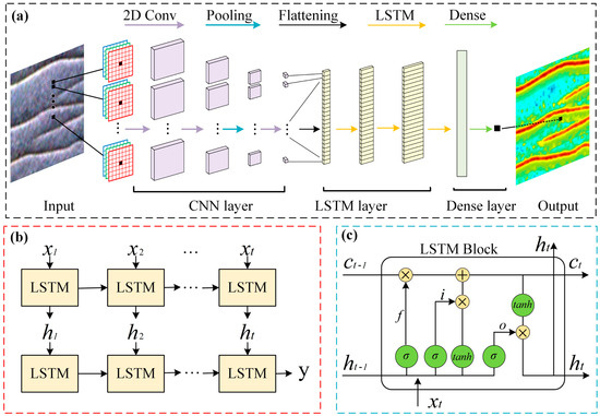
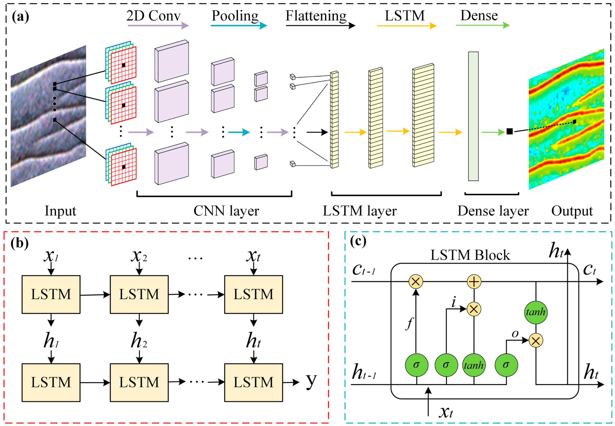
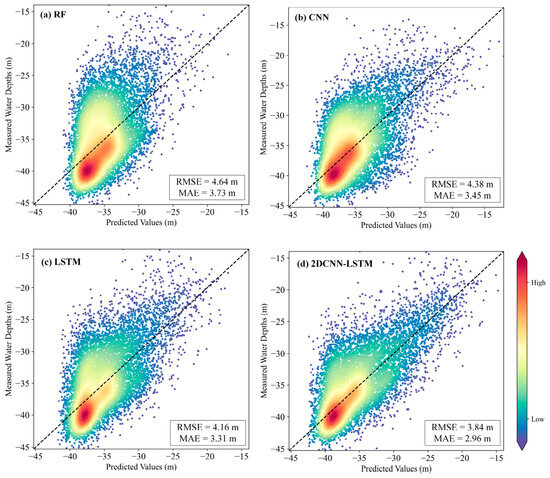
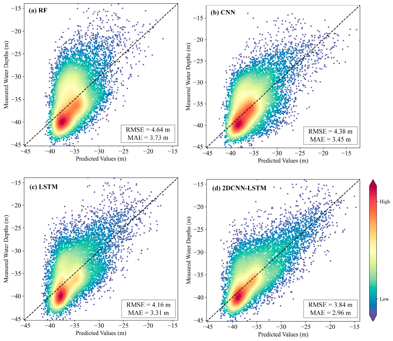
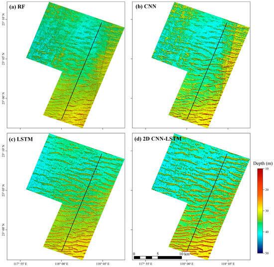
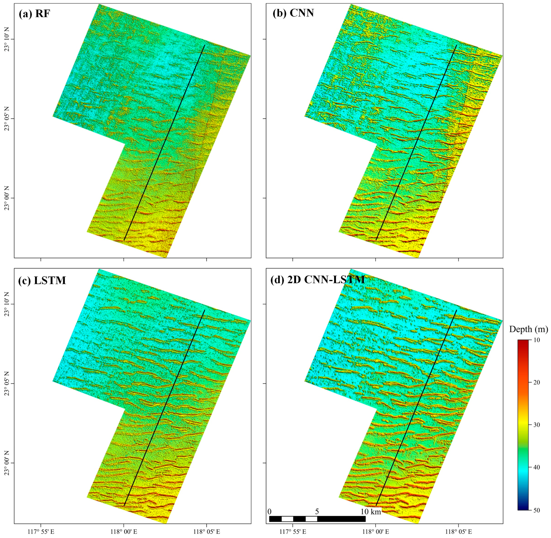
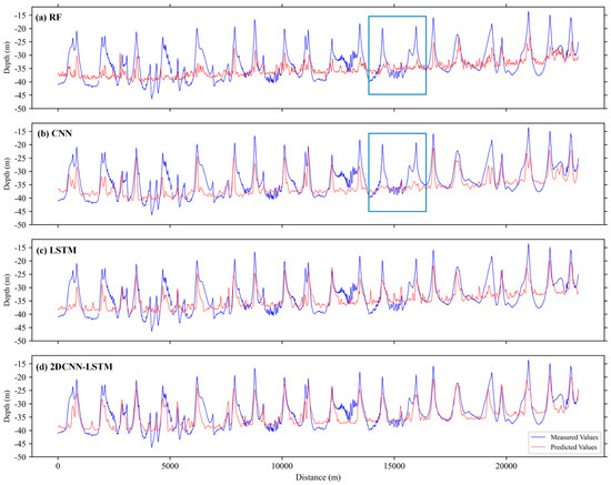
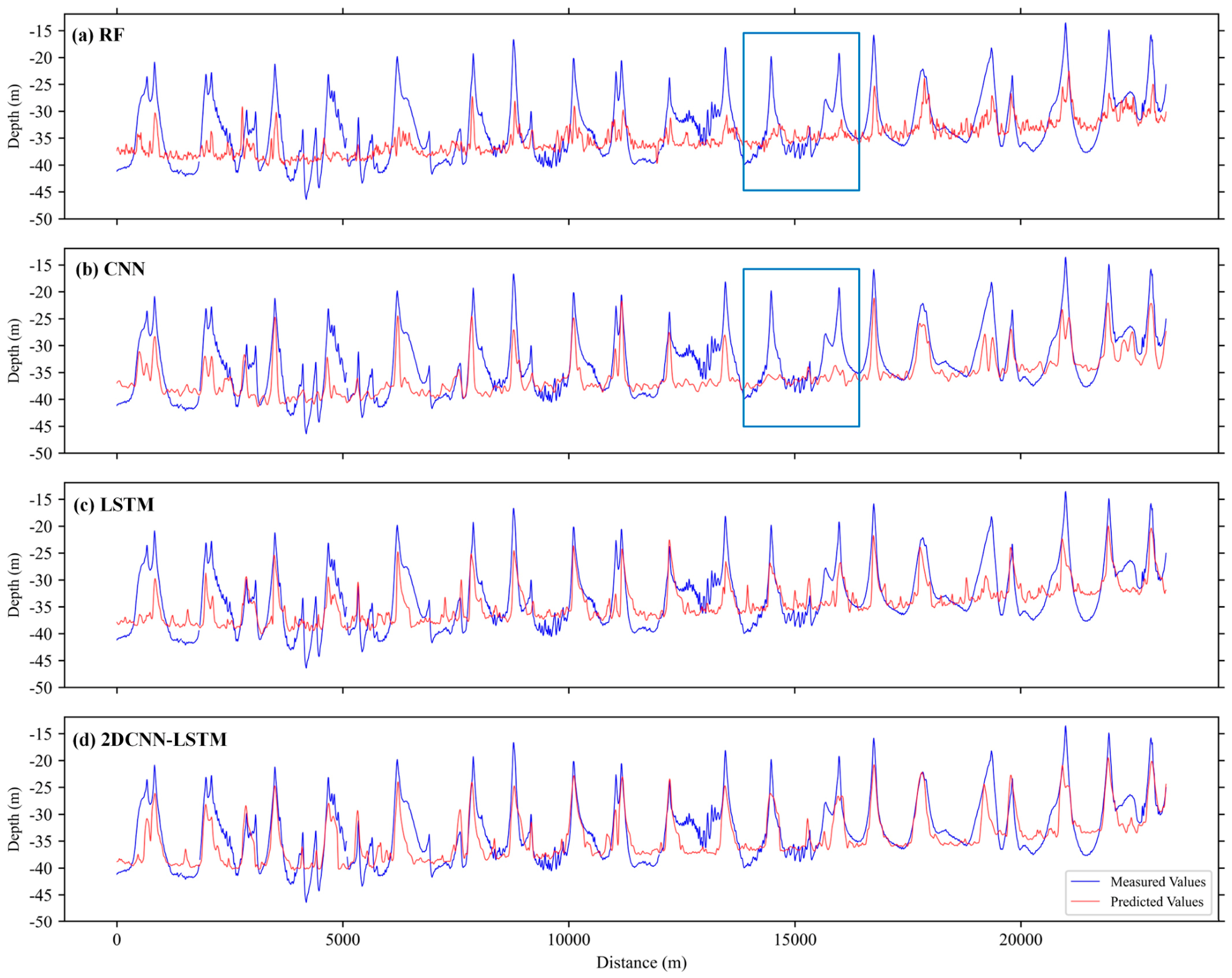
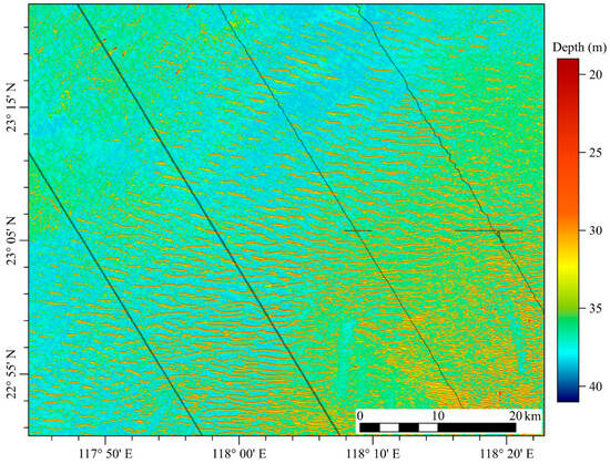
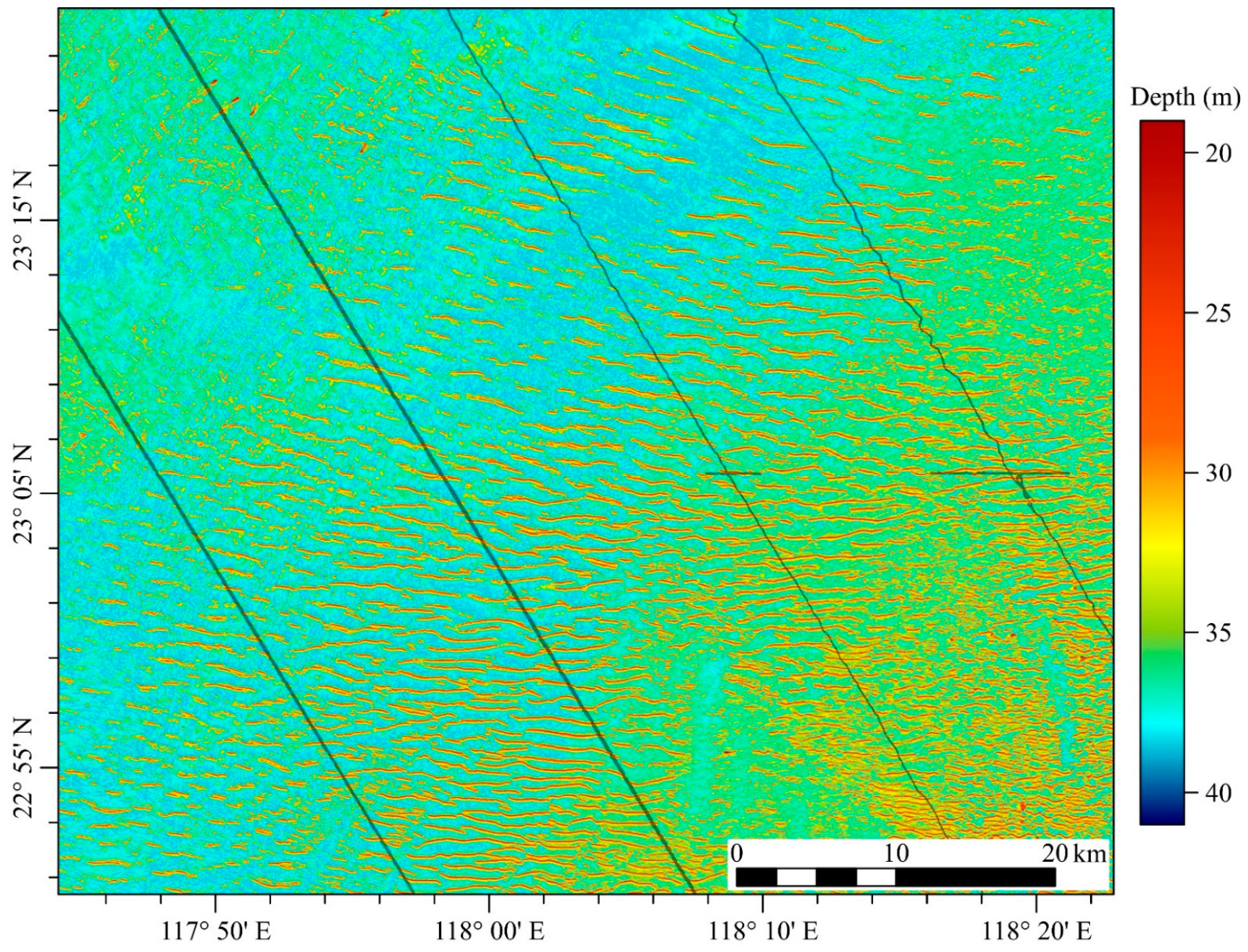
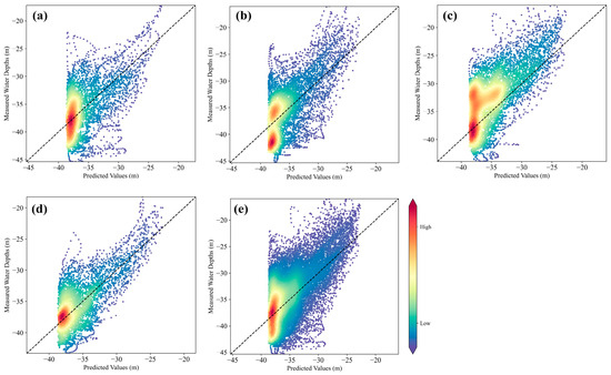
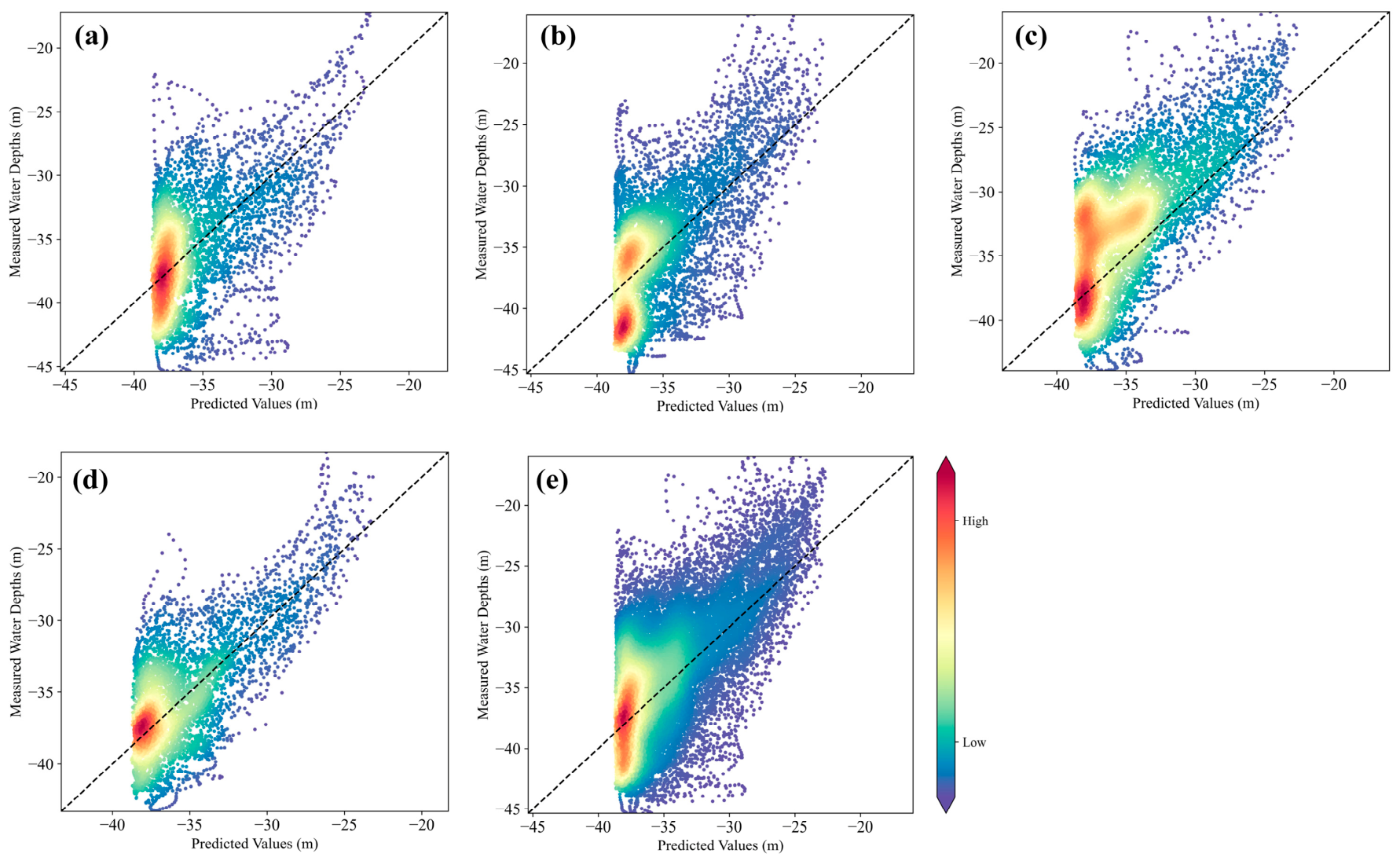
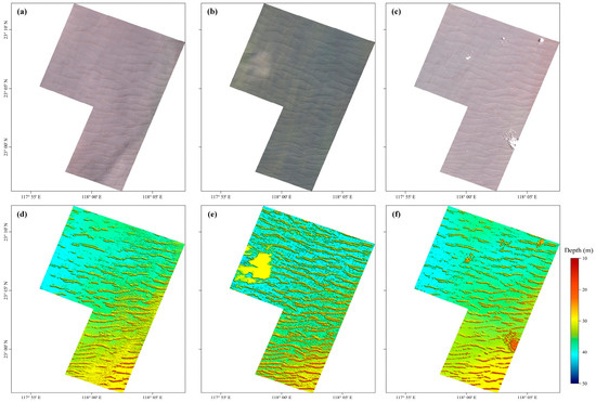
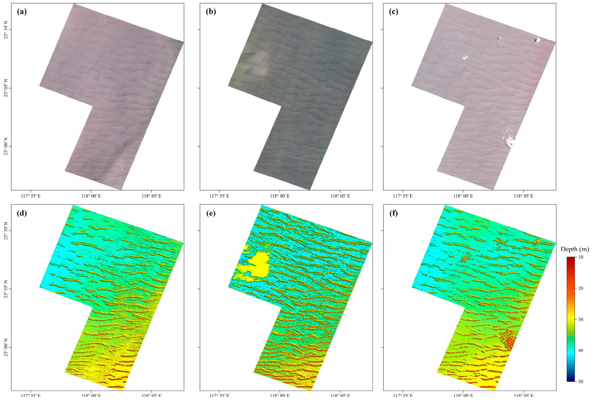
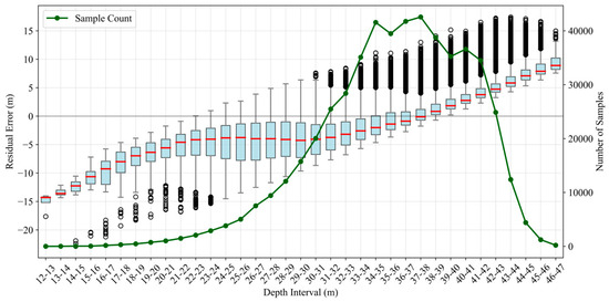
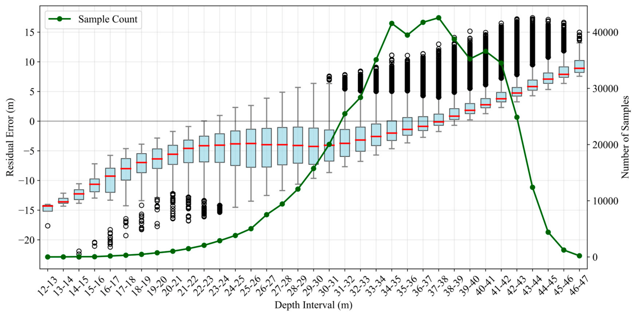
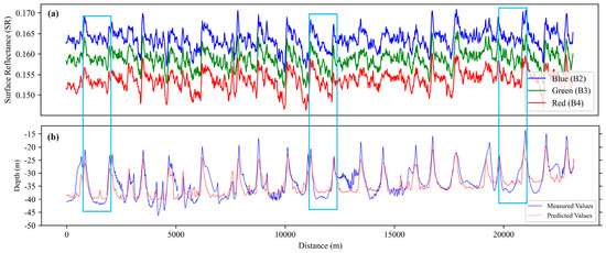
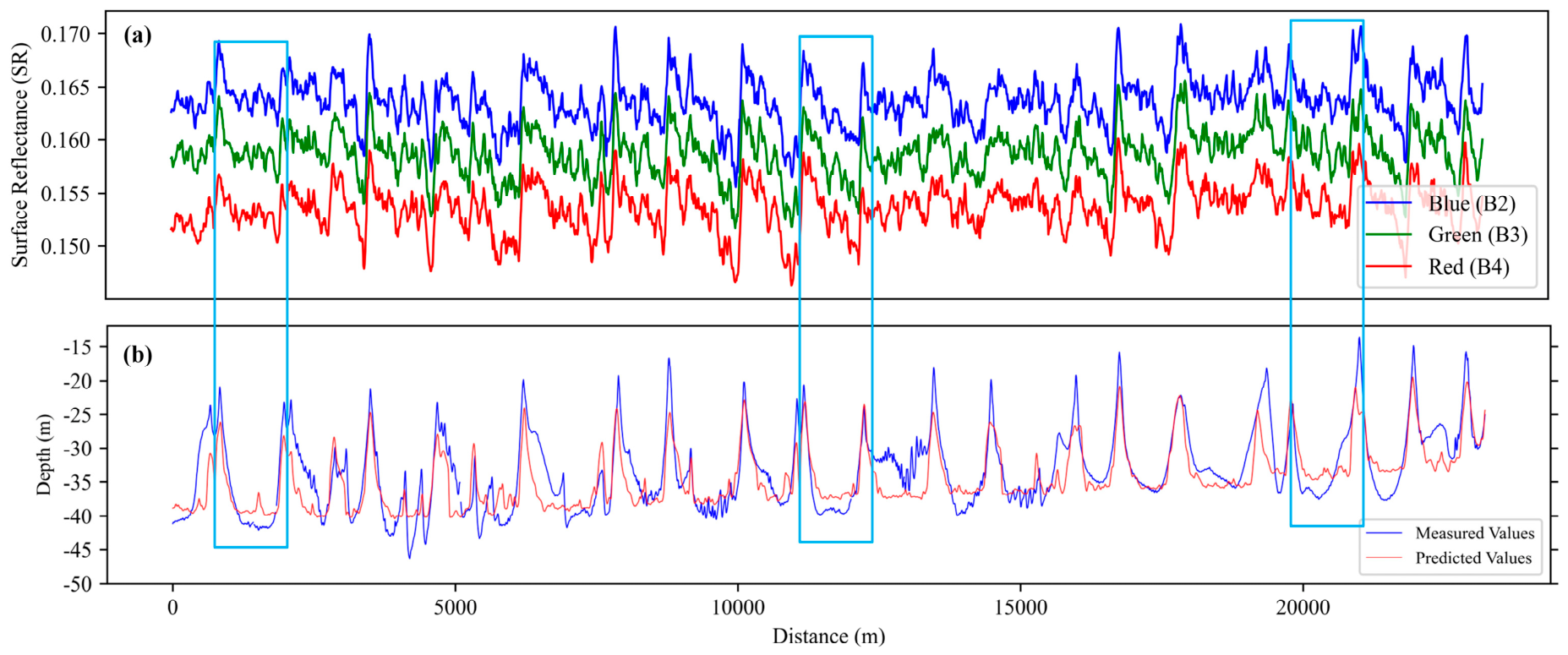
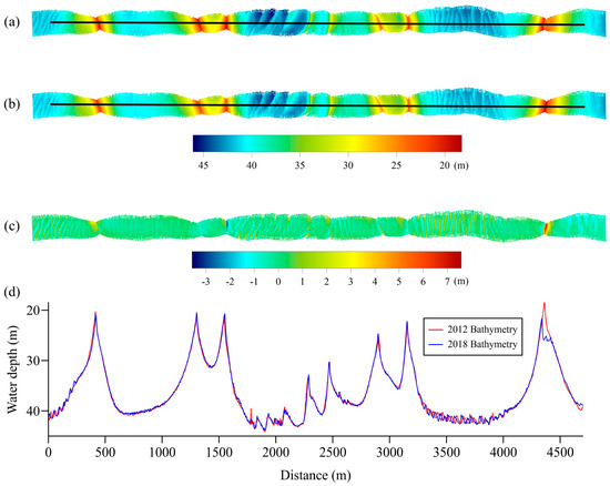
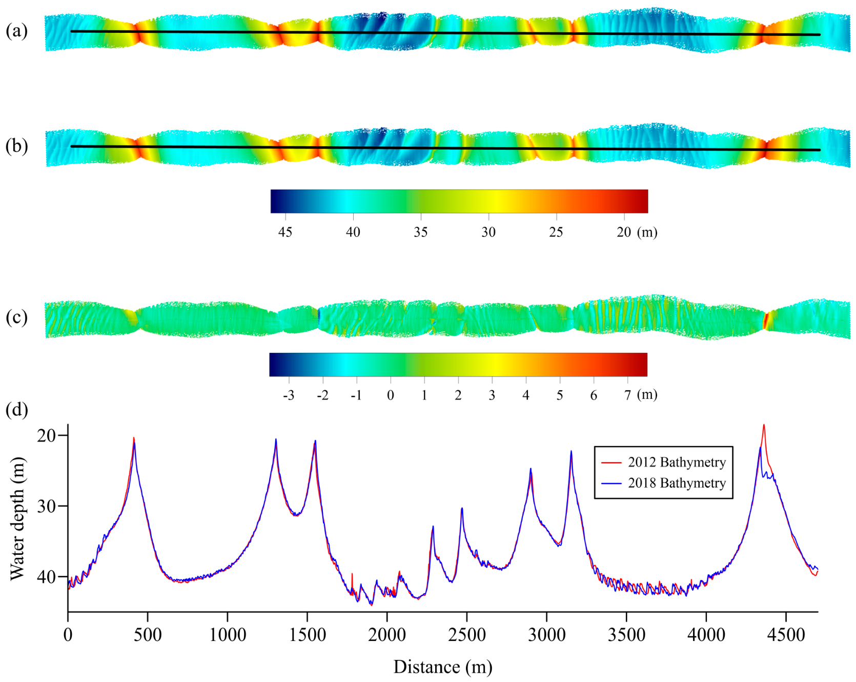

Disclaimer/Publisher’s Note: The statements, opinions and data contained in all publications are solely those of the individual author(s) and contributor(s) and not of MDPI and/or the editor(s). MDPI and/or the editor(s) disclaim responsibility for any injury to people or property resulting from any ideas, methods, instructions or products referred to in the content. |
© 2026 by the authors. Licensee MDPI, Basel, Switzerland. This article is an open access article distributed under the terms and conditions of the Creative Commons Attribution (CC BY) license.