


Highlights
What are the main findings?
- A continuity and label-constrained band selection method (CLBS) is proposed by integrating target–background contrast (TBC), target-region entropy (Entropy), and spectral–spatial contrast (SSC). Geometric mean fusion, a dynamic weighting mechanism, and a spectral continuity constraint are employed to jointly evaluate band quality and determine the retained band number.
- CLBS reduces the original 300 bands to 209, achieving a 30.3% dimensionality reduction while limiting the average number of spectrally continuous segments to 2.5449. Under the fixed training–validation split, it achieves an F1-score of 94.29%, a Precision of 100.00%, and a Recall of 89.19%. The ten-random-seed evaluation further yields average values of 94.96 ± 1.13%, 98.44 ± 1.65%, and 91.82 ± 3.31% for F1-score, Precision, and Recall, respectively.
What are the implications of the main findings?
- CLBS alleviates the conflict between dimensionality reduction and spectral continuity preservation, providing an interpretable band selection strategy that balances reduction efficiency, spectral feature retention, and underwater object type detection performance.
- A multi-category underwater debris hyperspectral dataset is constructed to alleviate data scarcity in underwater hyperspectral imaging. The current quantitative validation focuses on the two more established categories, metal and plastic, while the proposed framework may hold practical value for marine environmental monitoring, underwater debris cleanup, and marine resource exploration.
Abstract
Underwater object detection is a key technique for marine research. Traditional red green blue (RGB) imaging suffers from short detection ranges and serious color distortion in complex underwater environments. While hyperspectral images contain detailed spectral information, their high dimensionality increases computational costs and noise vulnerability, and high-quality underwater samples are difficult to obtain. A continuity and label-constrained band selection (CLBS) method is presented to address three common defects of existing underwater band selection techniques: target–background confusion, underutilization of spatial features and poor spectral continuity. Three metrics, namely target–background contrast (TBC), target region entropy (Entropy) and spectral–spatial contrast (SSC), are designed for band evaluation. Geometric mean fusion is adopted to suppress extreme values, and spectral continuity constraints are applied to determine the optimal band number. Meanwhile, a multi-category underwater hyperspectral dataset is constructed. Quantitative experiments are carried out on two fully annotated classes (metal and plastic). CLBS reduces the 300 original bands to 209, delivering a 30.3% dimensionality reduction with well-preserved spectral continuity. On a fixed train-validation partition, the 3DCNN+2DCNN model using CLBS-selected bands reaches an F1-score of 94.29%, a Precision of 100.00% and a Recall of 89.19%. Ten repeated tests with random seeds yield averaged results of 94.96 ± 1.13%, 98.44 ± 1.65% and 91.82 ± 3.31% for F1-score, Precision and Recall, respectively, demonstrating reliable performance. Comparative results show that CLBS outperforms conventional feature extraction and various supervised/unsupervised band selection methods. It achieves an excellent trade-off between dimensionality reduction and spectral feature preservation for underwater hyperspectral image processing.
1. Introduction
Underwater object type detection serves as a key enabling technology in marine-related fields, addressing bottlenecks in underwater information acquisition, replacing high-risk and low-efficiency manual diving inspections, and delivering essential data support for diverse applications such as marine engineering, ecological conservation, aquaculture, and the preservation of underwater cultural heritage. However, traditional red green blue (RGB) imaging faces inherent challenges in underwater object type detection scenarios: light absorption by water drastically shortens the imaging range and induces severe color distortion; light scattering from water and suspended particulates causes image blurring and significant contrast reduction and specific underwater targets, such as corroded metals and transparent plastics, tend to blend into complex backgrounds, hindering the extraction of discriminative features.
Hyperspectral imaging technology provides much higher spectral resolution than RGB imaging, with spectral coverage ranging from ultraviolet and visible light to near- and mid-infrared wavelengths, and divides the spectrum into tens to hundreds of contiguous narrow bands, thereby offering rich spectral information [1,2,3]. Compared with RGB images, the contiguous bands of hyperspectral images offer the following advantages: hyperspectral imaging is capable of capturing both spatial information and spectral characteristics of targets, enabling accurate target identification through continuous spectral information; the effects of underwater light absorption and scattering vary continuously with wavelength, and continuous spectra can comprehensively characterize this variation trend–based on continuous spectral data, algorithms can accurately model the continuous attenuation curves of water absorption and scattering, thereby effectively eliminating interference, whereas RGB imaging technology has difficulty faithfully restoring such continuous variations; from hyperspectral images, narrow bands with the strongest penetration capability can be selected, reducing unnecessary optical energy loss and significantly extending the imaging range, or alternatively, bands with strong absorption or scattering interference can be avoided, allowing image clarity to be maintained even in complex environments.
In the field of general object detection, extensive research has been conducted based on diverse imaging modalities and deep learning architectures, yielding notable performance in terrestrial and conventional scenarios [4]. For example, RGB-based detection models such as AGW-YOLOv8 and Feature-Adaptive FPN have shown strong capabilities in addressing occlusions, camouflage, and small object detection. Meanwhile, multi-modal fusion strategies integrating optical, acoustic, and laser imaging have further improved detection robustness in complex environments. However, these general methods are not directly tailored to underwater hyperspectral object type detection. In underwater scenes, wavelength-dependent light absorption and scattering weaken target responses and reduce image contrast, while suspended particles, illumination fluctuations, water turbulence, corrosion, and transparent materials further increase target–background ambiguity. These factors make it difficult to separate useful target spectra from background and environmental interference. In addition, hyperspectral images contain hundreds of contiguous narrow bands, which provide rich spectral information but also introduce high dimensionality, strong adjacent-band redundancy, and increased sensitivity to noise. If too many bands are retained, computational cost and low-quality information may increase; if too few bands are selected, the continuity of spectral responses may be disrupted. This is particularly important for underwater imaging because light attenuation and scattering vary continuously with wavelength. Therefore, underwater hyperspectral object type detection requires a band selection strategy that can reduce dimensionality while jointly considering target–background separability, spatial structural information, and spectral continuity.
Dimensionality reduction methods for hyperspectral images are broadly categorized into feature extraction (FE) and feature selection (FS) [5]. Specifically, FE projects original high-dimensional data into a low-dimensional subspace via mathematical transformations, generating novel composite features while retaining critical information. Representative feature extraction methods include principal component analysis (PCA), minimum noise fraction (MNF), linear discriminant analysis (LDA), and locally linear embedding (LLE). Researchers have also proposed improved variants based on these traditional methods. For example, Cao et al. [6] proposed a joint sparse local linear discriminant analysis (JSLLDA) method that integrates embedded regression and locality, incorporating regularization into the LDA model for hyperspectral image dimensionality reduction; Xue et al. [7] introduced functional principal component analysis (FPCA), which outperforms conventional methods in terms of classification accuracy, memory requirements, and execution time; Guan et al. [8] proposed a segmented minimum noise fraction-based method, which reduces transformation time while improving classification accuracy compared with the traditional MNF approach.
Feature selection, also referred to as band selection (BS), aims to select an optimal subset of bands from hundreds of original narrow bands through quantitative evaluation metrics. Currently, band selection methods are generally categorized into supervised, unsupervised, and semi-supervised approaches.
Supervised band selection utilizes training samples with known class labels to guide the band selection process. Such methods can be further divided into class separability-based approaches (e.g., JM distance and divergence), feature importance-based approaches, class label correlation-based approaches, and regularization-based approaches. Unsupervised band selection performs band selection without using any class label information, relying solely on the statistical properties, correlations, and information content of the data itself. Unsupervised methods include noise-based approaches, information-content-based approaches, correlation-based approaches, sparse representation-based approaches, clustering-based approaches, and manifold learning-based approaches. Semi-supervised band selection leverages a small number of labeled samples together with a large amount of unlabeled data by mining latent structures or discriminative information from the unlabeled samples. Mainstream semi-supervised band selection methods can be categorized into clustering-based, graph-based, and pseudo-label-based approaches. Guo et al. [9] proposed a two-stage unsupervised hyperspectral band selection method via deep reinforcement learning, which first filters high-noise bands by SNR thresholding and then optimizes band selection by modeling it as an MDP with an OIF-based reward function for SAC training. Hu et al. [10] demonstrated that a structural similarity ranking method (SSIM) outperforms entropy-based metrics, including entropy, relative Boltzmann entropy, and absolute Boltzmann entropy. Li et al. [11] and Fu et al. [1] both focused on the detection of sea cucumbers. The former adopted a two-stage selection strategy, where neighborhood optimization was performed via linear reconstruction in the first stage, followed by band elimination based on correlation quantification in the second stage; the latter achieved band selection through a combination of target constraints, K-means clustering-based decorrelation, and optimization of the optimal index factor (OIF). Due to their single-target focus and stringent real-time requirements, both methods retained only a small number of bands, which compromised spectral continuity and were unfavorable for multi-class object type detection. Wang et al. [12] assigned different weights to different regions through region segmentation and region-wise feature learning, and then efficiently reduced redundancy using K-means clustering and entropy-based measures. Patro et al. [13] formulated band selection as a dual-objective optimization problem by maximizing inter-cluster center distances in spectral clustering and the F-norm of spatially filtered bands, and solved it using parameter-free Jaya optimization.
To provide representative baselines for later comparison, several commonly used dimensionality reduction and band selection methods are also reviewed here. For standard feature extraction baselines, principal component analysis-based feature extraction (PCA-FE) [14], minimum noise fraction-based feature extraction (MNF-FE) [8], linear discriminant analysis-based feature extraction (LDA-FE) [15], and discrete wavelet transform-based feature extraction (DWT-FE) [16,17] are considered. Since these methods generate transformed components or coefficients, their outputs no longer directly correspond to original wavelengths. To further compare them under the original band selection setting, their adapted band selection forms are also considered, including principal component analysis based band selection (PCA-BS) [14], minimum noise fraction based band selection (MNF-BS) [8], linear discriminant analysis based band selection (LDA-BS) [15], and discrete wavelet transform based band selection (DWT-BS) [16,17]. In addition, maximum variance principal component analysis (MVPCA) [5], signal to noise ratio (SNR) [18], spectral angle distance (SAD) [19], Pearson correlation coefficient (PCC) [20], Euclidean norm (L2) [21], structural similarity index based ranking (SR-SSIM) [22], greedy selection based on structural similarity index (GS-SSIM) [22], and Jeffries–Matusita distance (JM) [23] are included as comparison methods.
Despite their high dimensionality reduction efficiency, FE methods generate features that are linear or nonlinear combinations of original spectral bands—features that may partially lose physical interpretability or fail to be directly linked to specific wavelengths [24,25]. In contrast, BS directly preserves the physical properties of original features without altering their intrinsic significance, thus demonstrating greater practical applicability. Supervised band selection methods, while optimizing downstream task performance, are prone to overfitting under limited underwater samples and usually suffer from high computational cost. Unsupervised methods exhibit stronger generalization ability and higher computational efficiency, but are vulnerable to noise and complex backgrounds, especially in turbid underwater imaging environments [26]. Moreover, underwater hyperspectral band selection still faces challenges such as target–background confusion, neglect of spatial characteristics, and degradation of spectral continuity caused by retaining too few bands and excessively pursuing low redundancy [27].
Based on the above analysis, an underwater hyperspectral image dataset is constructed and a continuity and label constraints-guided band selection (CLBS) and object type detection method is proposed. CLBS attempts to alleviate target–background confusion through a weakly supervised strategy using coarse labels, while explicitly incorporating spatial characteristics into the band selection process. The method incorporates three core metrics: target–background contrast (TBC), target region entropy (entropy), and spectral–spatial contrast (SSC). Finally, the number of selected bands is determined through a spectral continuity constraint.
The main contributions of this study are summarized as follows:
(1) A novel continuity and label-constrained band selection method, termed CLBS, is proposed for underwater hyperspectral object type detection. The method is designed to address target–background confusion, insufficient use of spatial characteristics, and degraded spectral continuity during band selection.
(2) Three band quality indicators, namely target–background contrast (TBC), target region entropy (Entropy), and spectral–spatial contrast (SSC), are constructed to evaluate bands from target–background separability, target-region information richness, and spectral–spatial discriminability. A geometric mean-based fusion strategy is further adopted to reduce the influence of extreme indicator values.
(3) A spectral continuity constraint is introduced to determine the final number of retained bands, enabling CLBS to reduce spectral dimensionality while preserving continuous spectral characteristics. This provides a balanced solution between dimensionality reduction efficiency and spectral feature retention.
(4) An underwater hyperspectral image dataset containing multiple underwater debris categories is constructed. The current quantitative validation focuses on the two more established categories, namely metal and plastic, and the experimental results demonstrate the effectiveness and stability of CLBS for underwater hyperspectral object type detection.
2. Materials and Methods
This section presents the proposed continuity and label-constrained band selection (CLBS) framework and its downstream object type detection model. The overall design of CLBS follows a two-stage strategy: first, a compact and physically interpretable subset of original spectral bands is selected under the joint consideration of target–background separability, label-guided discriminability, information richness, and spectral continuity; second, the selected band subset is fed into a 3DCNN+2DCNN model to verify its effectiveness for underwater object type detection.
The design philosophy of CLBS is to avoid relying on a single band-quality criterion. Specifically, target–background contrast (TBC) is used to measure the low-order radiance difference between the target and background regions, entropy is used to characterize the information richness within the target region, and spectral–spatial contrast (SSC) introduces label-guided spectral–spatial discriminability by combining target–background distribution separability and boundary response. These three complementary scores are fused using a geometric mean strategy, so that a band can obtain a high overall score only when it performs consistently well from multiple perspectives. A spectral continuity constraint is then introduced to determine the final number of retained bands and to avoid excessive fragmentation of the selected spectral subset. In this way, CLBS integrates band scoring, score fusion, continuity-constrained band subset determination, and downstream object type detection into a unified workflow.
2.1. Continuity and Label-Constrained Band Selection (CLBS)
This subsection first introduces three hyperspectral band evaluation metrics: target–background contrast (TBC), entropy, and spectral–spatial contrast (SSC). It then presents the overall score calculation method and the determination of the optimal number of bands based on spectral continuity.
2.1.1. Target–Background Contrast (TBC)
Target–background confusion is a common problem in underwater hyperspectral imaging because target responses are often weakened by light absorption, scattering, corrosion, and background interference. To quantify the discriminability between target and background regions, TBC is constructed by referring to the contrast-to-noise ratio (CNR) concept [28]. For the i-th band, measures the normalized radiance difference between the target and background regions. is calculated as shown in Equation (1):
where and denote the mean pixel values of the target and background regions in the i-th band, respectively; represents the standard deviation of the background region in the i-th band, and is a small positive constant used to avoid division by zero. The target and background regions are separated using the binary mask. After normalization, is used as one of the band quality scores. A larger value indicates stronger target–background separability and a lower relative influence of background fluctuation.
Within CLBS, TBC provides a low-order statistical cue for target–background separability. It is used together with Entropy and SSC so that the selected bands can simultaneously preserve target contrast, information richness, and spectral–spatial discriminability.
2.1.2. Entropy
Entropy complements TBC by capturing intra-target spectral variations that TBC alone cannot reflect. Meanwhile, since TBC is sensitive to noise, its score decreases under noisy conditions, preventing artificial inflation of the overall score caused by high entropy values induced by noise. For the i-th band, let X represent the set of pixel values within the target mask region. The value range of X is divided into 16 equal-width bins to balance spectral detail capture, statistical reliability, and computational cost. The normalized frequency corresponding to the k-th bin, denoted as , is calculated as shown in Equation (2):
where denotes the normalized frequency of the k-th bin in the i-th band, represents the number of pixels in the j-th bin (i.e., pixel value interval) of the i-th band (with corresponding to the pixel count of the k-th bin when ), and is a very small positive constant.
The entropy value of the i-th band is then calculated using Equation (3):
Finally, the entropy value of the i-th band is normalized via Equation (4) to obtain the corresponding entropy score:
A higher entropy score indicates richer spectral variation within the target region, which may reflect useful material details or discriminative target structures. Conversely, a lower entropy score suggests a relatively flat target response and limited contribution to band discrimination.
2.1.3. Spectral–Spatial Contrast (SSC)
In CLBS, the label constraint is introduced in the SSC calculation through the verified binary masks, which are used to distinguish target and background regions during band-quality evaluation. SSC is designed to jointly evaluate spectral separability and spatial edge response. It consists of three parts: spectral contrast (SC), spatial contrast (SPC), and a dynamic weighting strategy. SC measures the distribution difference between target and background pixels in the spectral domain, while SPC evaluates the boundary response of the target in the spatial domain.
- (a)
- Spectral Contrast (SC)
Based on label information, pixels in the target and background regions are extracted, denoted as the target pixel set T and background pixel set B, respectively. Histograms are computed for both T and B and then normalized into probability mass functions (PMFs), yielding and . Their calculations are shown in Equation (5):
where m denotes the index of the intensity interval (consistent with k in Equation (2)), represents the PMF value of the target pixel set T in the m-th intensity interval, is the number of pixels in T falling into the m-th intensity interval (i.e., the bin count of the target histogram), denotes the PMF value of the background pixel set B in the m-th intensity interval, and is the number of pixels in B falling into the m-th intensity interval (i.e., the bin count of the background histogram).
The Bhattacharyya distance is adopted as the separability measure. Equation (6) defines the Bhattacharyya coefficient (BC):
The calculation method of the Bhattacharyya Distance () is shown in Equation (7):
Finally, the Bhattacharyya distance is squared to further suppress bands with low discriminability while amplifying the advantages of highly discriminative bands, yielding the spectral contrast term SC. Its mathematical expression is given in Equation (8):
A larger SC value indicates a more pronounced distribution difference between the target and background in the corresponding band. Compared with TBC, which relies mainly on low-order statistics, SC describes target–background separability from the perspective of spectral probability distributions, making the two indicators complementary.
- (b)
- Spatial Contrast (SPC)
In addition to spectral separability, high-quality bands should also preserve clear spatial structures of the target. Therefore, SPC is introduced to evaluate the boundary response of the target region in each band.
In the first step, the target region mask (M) is extracted from label information. A morphological erosion operation is applied to obtain the eroded mask (), as expressed in Equation (9):
where ⊖ denotes the morphological erosion operator, B represents a structuring element with all elements equal to one and the origin at its center. Subsequently, the boundary mask () is derived by subtracting the eroded mask () from the original target mask (M), with its mathematical formulation given in Equation (10):
In the second step, Gaussian smoothing is applied to the entire original image of the i-th band () following Equation (11):
where ∗ denotes the convolution operation, is the original full image of the i-th band, represents a Gaussian kernel with standard deviation , and is the Gaussian-smoothed result of the entire i-th band image.
In the third step, the Sobel operator is used to compute the horizontal () and vertical () gradients of the Gaussian-smoothed image (), as defined in Equation (12):
where denotes the partial derivative with respect to the horizontal direction (i.e., x-axis) of the image, and denotes the partial derivative with respect to the vertical direction (i.e., y-axis). The gradient magnitude of the image is then calculated using Equation (13):
where represents the gradient magnitude of .
In the fourth step, the spatial contrast at target boundaries (denoted as ) is obtained by combining the boundary mask () and Equation (14):
where denotes the number of non-zero pixels in (i.e., the size of the boundary region), and represents the gradient of the Gaussian-smoothed i-th band image at pixel . A larger SPC value indicates that the corresponding band provides a clearer target boundary response, which can help preserve spatial structural information during band selection.
- (c)
- Dynamic Weighting of SC and SPC
In the computation of spectral–spatial joint contrast (SSC), the spectral contrast (SC) and spatial contrast (SPC) terms are fused to optimize band selection. The core weighting formula is given in Equation (15):
The weighting coefficient is dynamically determined based on the spectral discriminability indicator (TBC). When the TBC value is high, greater emphasis is placed on the spectral contrast term (SC); conversely, when the TBC value is low, more weight is allocated to the spatial contrast term (SPC). Additionally, is constrained within the range —this constraint balances the contributions of the two terms and avoids instability in band selection caused by extreme weight fluctuations. This range is selected based on practical engineering considerations, with the primary objective being to prevent extreme weight allocation; the specific boundary values are not intended to represent precise thresholds. The mathematical formulation of this constraint is provided in Equation (16):
2.1.4. Overall Band Scoring and Retained Band Number Determination
After TBC, Entropy, and SSC are calculated for each spectral band, an overall score is required to integrate these complementary band-quality cues into a single ranking criterion. This overall score is used to rank all candidate bands according to their joint target–background separability, target-region information richness, and spectral–spatial discriminability.
Before score fusion, the three indicators are normalized across all candidate bands to make their numerical ranges comparable. In the proposed CLBS framework, geometric mean fusion is adopted as the default overall score computation strategy. Arithmetic mean, harmonic mean, and CRITIC-weighted sum are evaluated as alternative fusion strategies in the ablation experiments to examine the influence of different score aggregation schemes.
- (a)
- Weighted-Sum Method
The overall score calculated using arithmetic mean weighting is given in Equation (17):
Alternative weighting schemes, for example, the linear combination formula in Equation (18), are also available, with the linear combination formulation expressed as follows:
However, due to the complexity of samples (as well as variations in illumination conditions and water environments), determining a fixed set of coefficients a, b, and c for this scheme remains challenging.
- (b)
- Harmonic Mean Method
The harmonic mean is also considered because it assigns stronger penalties to low indicator values. It is calculated as follows:
where is the same small positive constant used to avoid division by zero. This strategy emphasizes balanced performance among the three indicators and suppresses bands with extremely low values in any individual metric.
- (c)
- CRITIC-Weighted Sum Method
Considering that TBC, Entropy, and SSC may not be completely independent, a CRITIC-weighted sum is introduced as a correlation-aware scoring strategy. For the j-th indicator, its information content is calculated as follows:
where denotes the standard deviation of the j-th indicator, and denotes the Pearson correlation coefficient between the j-th and k-th indicators. The corresponding weight is then defined as follows:
The CRITIC-weighted score is calculated as follows:
Unlike fixed-weight strategies, CRITIC considers both the variation in each indicator and the correlation among indicators.
- (d)
- Geometric Mean Method
Geometric mean fusion is used as the default score computation method in CLBS. Here, TBC, Entropy, and SSC denote the normalized indicator values. To reduce the influence of unbalanced indicator values, the overall score based on the geometric mean is formulated in Equation (23):
Compared with the arithmetic mean, the geometric mean emphasizes the joint balance among the three indicators. A band can obtain a high overall score only when it performs reasonably well in target–background contrast, target-region information richness, and spectral–spatial contrast. Therefore, this strategy helps suppress bands whose high score is caused by only one abnormal indicator.
- (e)
- Quantification of Spectral Continuity
The core of spectral continuity quantification lies in calculating the number of contiguous segments within the selected band index sequence. For a sorted set of band indices, a contiguous segment is defined as a maximal consecutive subsequence where the difference between adjacent indices equals 1. The count of such maximal subsequences is equivalent to the number of contiguous band segments, denoted by C. For example, for the band index sequence , there are three maximal contiguous subsequences: , , and . The number of contiguous segments serves as an intuitive metric for spectral continuity: fewer segments indicate better spectral continuity.
- (f)
- Number of Retained Bands
For hyperspectral image datasets, all samples should retain the same number of bands to ensure data alignment. Therefore, the average number of contiguous band segments across the dataset is used to evaluate the overall spectral continuity under different retained band numbers. The original dataset contains 300 bands. Retaining too many bands weakens the effect of dimensionality reduction, whereas retaining too few bands may discard useful spectral information. Therefore, the candidate range of retained bands is set to .
Consider a dataset containing N hyperspectral samples. For the q-th sample, suppose its band selection result corresponds to an index set consisting of h bands, denoted as . The mathematical expression of this set is given in Equation (24):
where (for ) represents the i-th band index in the selection result of the q-th sample. By iterating over values of h within the range , the average number of contiguous segments for the dataset under different retained band counts is computed, as expressed in Equation (25):
where represents the number of contiguous subsequences (i.e., the number of contiguous band segments) within the index set —which contains h retained bands and corresponds to the q-th sample in the dataset—and N denotes the total number of hyperspectral samples in the dataset. Additionally, denotes the average number of contiguous band segments across the entire dataset when h bands are retained. The value of h that minimizes the average number of contiguous segments across the dataset is selected as the final number of retained bands (ensuring optimal spectral continuity), denoted as . Its calculation formula is expressed in Equation (26):
where represents the number of retained bands corresponding to optimal spectral continuity, and denotes the value of the variable (here, h) that minimizes the subsequent expression.
2.1.5. Band Selection Process
The overall band selection pipeline is illustrated in Figure 1. First, original hyperspectral images (comprising 300 bands) are fed into the pipeline; the TBC, entropy, and SSC metrics of each band are computed to derive an overall score per band, and these scores are sorted in descending order. Next, the optimal number of retained bands is determined iteratively: initialize h to 150, select the top h bands ranked by their overall scores, and calculate the average number of contiguous segments of the selected bands to characterize the spectral continuity of the dataset under this retained band count. h is incremented by 1 in each iteration, resulting in a total of 101 iterations (with ). Subsequently, upon completion of all iterations, the h value corresponding to the minimum average number of contiguous segments (i.e., optimal spectral continuity, ) is selected as the final number of retained bands. Finally, the top 209 bands (ranked by their overall scores in descending order) are selected and then reordered according to their original wavelength indices to form the final dataset. To further improve readability and reproducibility, the complete CLBS workflow is summarized in Algorithm 1.
| Algorithm 1 Workflow of the proposed CLBS framework. |
| Input: Underwater hyperspectral dataset X with spectral bands; verified binary masks M; candidate retained-band range , where and . |
| Output: Selected band subset and the reduced hyperspectral dataset for downstream object type detection. |
|
Figure 1.
Band selection flowchart for hyperspectral images.
2.2. Sample Augmentation
After the CLBS-selected band subset is obtained, training augmentation is applied to improve the robustness of the downstream detector under complex underwater hyperspectral imaging conditions. In underwater scenes, target appearance and spectral responses may vary due to changes in imaging viewpoint, target pose, local occlusion, illumination fluctuation, water scattering, sensor noise, and band-wise response variation. Therefore, a joint spatial–spectral augmentation strategy is adopted to simulate these practical disturbances during training while preserving the physical meaning of spectral information. Data augmentation is applied only to the training set, while the validation set remains unchanged to ensure an unbiased evaluation. In the training stage, both the original training samples and the augmented training samples are used. For each augmented training sample, spatial and spectral augmentation operations are independently triggered with a probability of 50%. During spatial augmentation, the hyperspectral image and its corresponding mask are transformed synchronously to maintain consistency between the target region and spectral data. During spectral augmentation, only the hyperspectral image is modified, while the mask and class label remain unchanged.
The augmentation strategy includes random rotation, random flipping, random cropping with size restoration, Gaussian noise injection, and band-wise scaling. These operations can generate multiple augmentation combinations, thereby increasing training sample diversity while maintaining data realism.
In implementation, an augmented candidate set is first generated from the original training set. If no effective augmentation operation is applied to a candidate sample, this unchanged duplicate is excluded from the augmented set to avoid introducing repeated samples. The remaining augmented samples are then concatenated with the original training samples, and the combined training set is randomly shuffled during mini-batch loading. Therefore, data augmentation increases the diversity of training samples without changing the validation protocol.
2.2.1. Spatial Augmentation
Spatial augmentation operates primarily on the spatial dimension of images, simulating variations in target position, orientation, and scale that may occur in real underwater environments. For each augmented training sample, the following geometric transformations are applied probabilistically.
Random rotation: The image and its corresponding mask are rotated by , , , or . Rotation augmentation helps the model learn rotational invariance and prevents overfitting to specific orientations.
Random flipping: The image and mask are flipped horizontally and/or vertically. Random flipping simulates mirror-like appearances caused by water currents, sedimentation, or varying imaging viewpoints in underwater environments. For targets with weak symmetry, random flipping serves as an efficient augmentation strategy.
Random cropping with size restoration: A subregion is randomly cropped at a ratio of of the original image size. Bilinear interpolation is used to resize the image back to its original dimensions, while nearest-neighbor interpolation is applied to the mask to avoid label contamination. Random cropping and size restoration simulate partial occlusion and scale variations while introducing mild deformations, thereby improving robustness to non-rigid distortions.
2.2.2. Spectral Augmentation
The core advantage of hyperspectral images lies in their rich spectral information. Spectral augmentation is used to simulate spectral disturbances commonly observed in underwater hyperspectral imaging, including illumination fluctuation, water-induced scattering and absorption variation, sensor noise, and band-wise response drift. These operations encourage the detector to learn more robust spectral–spatial representations from the CLBS-selected bands.
Gaussian noise injection: Zero-mean Gaussian noise with a standard deviation of is added to all spectral bands. Underwater imaging is often affected by scattering, absorption, and sensor noise; noise injection improves the model’s tolerance to low-quality spectral signals, preventing the model from over-relying on subtle spectral differences present only in low-noise data.
Band-wise scaling: Each spectral band is independently multiplied by a random scaling factor within the range . Band-wise scaling simulates illumination intensity variations caused by depth changes and models sensor response drift.
2.3. 3DCNN+2DCNN Hybrid Model for Downstream Detection
After the CLBS-selected band subset is obtained, a downstream object type detection model is required to evaluate whether the selected bands provide effective spectral–spatial information for underwater target discrimination. The 3DCNN+2DCNN model is used to verify the detection effectiveness of the selected bands rather than to introduce additional label constraints into the network architecture. To validate the effectiveness of the proposed band selection method, a hybrid three-dimensional and two-dimensional convolutional neural network (3DCNN+2DCNN) is adopted as the object type detection backbone [29]. Hyperspectral images contain both spectral and spatial information. A conventional 2DCNN can effectively extract spatial features, but it cannot directly model local correlations along the spectral dimension. In contrast, a 3DCNN can jointly capture spectral–spatial features, but using a deep 3DCNN alone may introduce high computational cost and increase the risk of overfitting under limited underwater hyperspectral samples. Therefore, a stage-wise hybrid structure is used in this study: a lightweight 3D convolutional block first extracts local spectral–spatial features from contiguous spectral neighborhoods, and subsequent 2D convolutional layers further refine spatial feature representations.
The architecture of the 3DCNN+2DCNN model is illustrated in Figure 2. The input of the network is the hyperspectral image after CLBS band selection, with 209 retained bands and a spatial size of . The 3D convolutional block is placed at the front of the network. It uses a convolution kernel of size with 16 output channels. The stride is set to , where the stride of 1 along the spectral dimension enables the convolution kernel to slide continuously over the selected bands, while the stride of 2 along the spatial dimensions reduces computational cost through early spatial downsampling. After 3D convolution and 3D max pooling with a kernel size of , the output feature tensor has the size .
Figure 2.
Architecture of the 3DCNN+2DCNN hybrid model. The selected hyperspectral bands are first processed by a lightweight 3D convolutional block to extract local spectral–spatial features. The 5D feature tensor is then reshaped into a 4D tensor by encoding spectral–spatial responses into the channel dimension, followed by 2D convolution, global pooling, and classification.
The reduction in the spectral feature depth in this stage is performed on learned feature responses rather than on the original spectral bands. Specifically, all 209 selected input bands participate in the initial 3D convolution, and the subsequent 3D max pooling locally aggregates adjacent spectral–spatial feature responses. Thus, the 3D block uses the continuous spectral information preserved by CLBS to form compact local spectral–spatial representations.
To connect the 3D and 2D convolutional modules, the 5D tensor is reshaped into a 4D tensor . This operation merges the 3D output channel dimension and the spectral feature depth, where , while keeping the spatial dimensions unchanged. Therefore, the learned spectral–spatial responses are encoded into the channel dimension and then processed by the following 2D convolutional layers.
The 2D convolutional module contains three convolutional layers. The first 2D convolution reduces the number of channels to 32, the second layer increases the channel number to 64, and the third layer further increases it to 128. Each 2D convolutional layer is followed by Group Normalization, ReLU activation, and max pooling. The spatial resolution is gradually reduced from to , , and after the three pooling operations.
Group Normalization (GN) is used instead of Batch Normalization to improve training stability under small-batch conditions. In this study, the batch size is set to 1; therefore, batch-dependent statistics may be unstable. GN normalizes features within channel groups and is less sensitive to the batch dimension. In the 3D convolutional block, the 16 output channels are divided into 4 groups. In the 2D convolutional and fully connected layers, eight groups are used when the channel number is divisible by 8.
Finally, global pooling is applied to convert the feature maps into a spatial resolution, producing a feature tensor of size . The tensor is flattened into a 2048-dimensional feature vector and fed into the classifier. The classifier consists of two fully connected layers and an output layer, following the structure FC, FC, and FC, where denotes the number of object categories. Dropout with a rate of 0.5 is used in the fully connected layers, and the final output layer predicts the object category of each input sample.
3. Results
To verify the effectiveness of the proposed CLBS method, a series of experiments was conducted on a self-built underwater hyperspectral dataset. The following subsections sequentially present the dataset details and preprocessing, experimental configuration, band selection performance, and comparative analysis results.
3.1. Dataset
Given the scarcity of existing research on underwater hyperspectral imaging and the scarcity of publicly available underwater hyperspectral datasets, we devoted considerable effort to constructing the underwater hyperspectral dataset presented in this paper. Imaging was performed using a FigSpec FS-23 hyperspectral camera (Hangzhou CHNSpec Technology Co., Ltd., Hangzhou, China). This camera integrates a high-diffraction-efficiency transmissive grating spectroscopic module with a high-sensitivity area-array detector and is equipped with built-in scanning imaging functionality and an auxiliary camera. Detailed specifications are as follows: image resolution of , spectral range of 400–1000 nm, spectral resolution of 2.5 nm, dynamic range of 12 bits, pixel size of , CMOS detector, and built-in battery power supply. Data acquisition was conducted under varied underwater imaging conditions. For natural-light scenes, samples were collected between 10:00 AM and 3:00 PM under sunny and cloudy weather conditions, covering both strong and weak daylight. In addition, samples were also collected under supplemental-lighting conditions without direct natural sunlight, including full-spectrum and infrared illumination. The data were collected in a shallow underwater setting, with the water depth varying within approximately 1 m. During acquisition, the target placement, imaging distance, and illumination conditions were varied to increase scene diversity.
The raw data comprise 300 spectral bands, each with pixels, and were calibrated using an underwater calibrated reflectance white reference panel. During the initial preprocessing stage, the spatial size was cropped to pixels while maintaining the original number of bands.
The constructed underwater hyperspectral dataset contains multiple categories of underwater debris, including metal, plastic, glass, rubber, fabric, and other object types. Representative examples of several categories are shown in Figure 3. Among these categories, metal and plastic have been collected and annotated more systematically, with relatively sufficient sample sizes and richer subtype coverage. Categories such as glass, rubber, and fabric have also been included in the ongoing dataset construction; however, they are still being further expanded and organized in terms of sample scale, subtype diversity, and annotation consistency.
Figure 3.
Representative examples of different categories in the constructed underwater hyperspectral dataset, including metal, plastic, glass, rubber, and fabric.
Considering sample balance, category representativeness, and experimental rigor, the current quantitative experiments focus on the two more established categories, namely metal and plastic. The quantitative subset used in this study contains more than 600 hyperspectral samples from the metal and plastic categories in total, with an approximately 1:1 sample ratio between the two categories. Metal samples include common materials such as cast iron, alloy steel, aluminum and aluminum alloys, copper and copper alloys, and stainless steel. These metal samples exhibit varying degrees of corrosion, including non-corroded, slightly corroded, moderately corroded, and severely corroded states.
Due to differences in material density, plastic objects may either float or sink in water. In this dataset, all plastic samples used in the current experiments exhibit sinking behavior: most have densities greater than that of water; a small number have densities lower than that of water but sink due to contamination with impurities, such as mud and gravel, rendering the samples more representative of real-world underwater plastic debris. Plastic samples include transparent, white, black, and colored plastics.
The label data were manually annotated using LabelMe on pseudo-color images generated from the hyperspectral data. During annotation, the reference physical samples and the corresponding pixel locations in the raw hyperspectral images were jointly considered to delineate target regions and generate binary masks. To improve label reliability, the annotation results were further checked by multiple researchers through secondary inspection. Uncertain or inconsistent annotations were corrected by re-examining the original physical samples, pseudo-color images, and corresponding hyperspectral image regions. For the current quantitative experiments, the verified binary masks corresponding to the metal and plastic samples are used to separate target and background regions during band quality evaluation.
3.2. Experimental Setup
This section presents the comparative experiments and ablation experiments designed to evaluate the proposed method, along with the metrics adopted for assessing detection performance. The comparative experiments include retained band number comparison, overall score calculation strategy comparison, and comparison with other dimensionality reduction and band selection methods. In addition, ablation experiments are conducted to evaluate the contributions of the proposed indicators, the sensitivity of the constraint range, and the influence of different detection model backbones.
3.2.1. Comparative Experiments
To evaluate the effectiveness of the proposed continuity and label-constrained underwater hyperspectral band selection method, comparative experiments are divided into three groups.
In the first group, detection accuracy is compared under different numbers of retained bands using the same detection model. The tested numbers of retained bands include 100, 150, 200, 209, 250, and all 300 original bands.
In the second group, different overall score calculation strategies are compared, including arithmetic mean, harmonic mean, CRITIC-weighted sum, and geometric mean. This group of experiments is designed to evaluate the robustness and rationality of the geometric mean-based fusion strategy.
The third group compares CLBS with representative dimensionality reduction and band selection methods. These methods are divided into four categories according to their output forms and use of supervision: standard feature extraction methods, adapted feature-extraction-based band selection methods, unsupervised band selection methods, and supervised band selection methods. This grouping allows the comparison to separately examine the effects of transformed feature representation, original-band interpretability, unsupervised selection, and label-guided separability.
The first category consists of standard feature extraction methods, including PCA-FE, MNF-FE, LDA-FE, and DWT-FE. PCA-FE projects the original spectral data into principal components with large variance, MNF-FE emphasizes components with higher signal-to-noise quality, LDA-FE extracts discriminative components according to class separability, and DWT-FE represents spectra using wavelet coefficients along the spectral dimension. These methods are included to examine whether transformed spectral features can provide effective information for underwater object type detection. Compared with these methods, CLBS retains original wavelength bands and, therefore, preserves direct spectral interpretability.
The second category consists of adapted feature-extraction-based band selection methods, including PCA-BS, MNF-BS, LDA-BS, and DWT-BS. Instead of directly using transformed components, these methods estimate the importance of original bands according to the loadings, discriminant weights, or energy responses generated by the corresponding feature extraction methods. They are included to provide a more direct comparison with CLBS under the original-band selection setting and to examine whether classical feature-transformation criteria can effectively identify useful original wavelengths.
The third category consists of representative unsupervised band selection methods, including MVPCA, SNR, SAD, PCC, L2, SR-SSIM, and GS-SSIM. MVPCA ranks bands according to variance-related information; SNR selects bands with stronger signal quality, SAD and PCC evaluate spectral distance or correlation relationships among bands, L2 measures band energy strength, and SR-SSIM and GS-SSIM select bands according to structural similarity and redundancy. These methods are included because they mainly rely on intrinsic spectral or spatial statistics without using target–background supervision. Comparing CLBS with this category can evaluate whether label-guided band-quality assessment is beneficial in underwater scenes with target–background ambiguity.
The fourth category consists of the supervised JM-distance-based band selection method. JM measures class separability using label information and is, therefore, included as a supervised separability baseline. Comparing CLBS with JM can further examine whether combining target–background separability, target-region information richness, spectral–spatial discriminability, and spectral continuity provides advantages over a single supervised separability criterion.
All compared methods are evaluated under the same training and evaluation protocol. For methods that output original wavelength bands, the selected bands are used as the input of the downstream 3DCNN+2DCNN detection model. For standard feature extraction methods that output transformed components or coefficients, the input spectral dimension of the detection model is adjusted according to the corresponding output features. This setting ensures that the comparison mainly reflects the effect of different spectral dimensionality reduction and band selection strategies rather than differences in the downstream detector.
3.2.2. Evaluation Metrics
In this study, Precision, Recall, and F1-score (F1) are adopted as evaluation metrics, with plastic samples designated as the positive class (1) and metal samples as the negative class (0). Precision is defined as the proportion of true positive samples among all samples predicted as positive. Recall represents the proportion of true positive samples correctly identified among all actual positive samples. The F1-score is the harmonic mean of Precision and Recall, placing greater emphasis on the lower value of the two.
3.2.3. Implementation Details and Training Parameters
All experiments were implemented using PyTorch 1.8.1 and conducted under the same training and evaluation protocol. The dataset was divided into training and validation subsets with a ratio of 8:2, and a fixed random seed was used to ensure reproducibility. The same data partition was adopted for all comparative experiments to ensure fairness. Data augmentation was applied only to the training set, while the validation set was kept unchanged.
The 3DCNN+2DCNN model was trained with a batch size of 1. The maximum number of training epochs was set to 50, and an early stopping strategy was adopted to prevent overfitting. Specifically, training was terminated if the validation performance did not improve for 10 consecutive epochs. The Adam optimizer was used with an initial learning rate of 0.001. A ReduceLROnPlateau learning rate scheduler was adopted to reduce the learning rate when the validation loss stopped decreasing, with a patience of 5 epochs and a reduction factor of 0.5. Focal loss was used as the training loss function, and the focusing parameter was set to 2. The experiments were conducted on an NVIDIA GeForce RTX 2080 Ti GPU.
For all band selection methods, the selected original bands were used as the input of the same 3DCNN+2DCNN model. For standard feature extraction methods, including PCA-FE, MNF-FE, LDA-FE, and DWT-FE, the transformation parameters were estimated only from the training data and then applied to the validation data to avoid information leakage. The input spectral dimension of the detection model was adjusted according to the number of transformed features produced by each feature extraction method.
3.3. Results of the Band Selection Module
The performance of the band selection module is evaluated using the three constructed key metrics (TBC, Entropy, SSC). Detailed results of band overall scores and optimal retained band numbers are presented in the following subsections.
3.3.1. Band Overall Score
- (a)
- Arithmetic Mean-Based Scoring Strategy
A metal sample was randomly selected. The arithmetic mean-based overall scores and the individual indicator scores for each band of this sample are shown in Figure 4, where the horizontal axis denotes the band index and the vertical axis denotes the score. The grayscale images of band 15 and band 122 are shown in Figure 5. The arithmetic mean overall score of band 15 is 0.470005, whereas that of band 122 is 0.470385.
Figure 4.
The horizontal axis represents all 300 bands of a hyperspectral image, with the spectral range from 400 nm to 1000 nm. The vertical axis denotes the score calculated by the arithmetic mean method, as defined in Equation (17).
Figure 5.
Metal sample images at two different bands, (a) band 15 and (b) band 122.
According to the arithmetic mean-based scoring scheme, bands 15 and 122 exhibit very similar scores, suggesting that their grayscale images should be visually comparable. However, visual inspection of the grayscale images clearly indicates that band 15 is substantially superior to band 122. This demonstrates that the arithmetic mean-based overall scoring strategy fails to reliably reflect band quality. Further analysis reveals that band 15 exhibits relatively balanced values across the three indicators. In contrast, band 122 has an abnormally high TBC value, resulting in extreme-value interference that inflates its overall score. Since different samples may exhibit peak values at different bands, a weighted arithmetic strategy is difficult to generalize effectively across all data.
- (b)
- Geometric Mean-Based Scoring Strategy
The geometric mean-based overall scores and individual indicator scores for each band of Figure 4 are presented in Figure 6, with the vertical axis representing the score and the horizontal axis denoting the band index. The geometric mean-based overall score of band 15 is , which is lower than its arithmetic mean score. In contrast, the geometric mean-based overall score of band 122 decreases to , representing a reduction of compared with its arithmetic mean score. The overall scores derived from the geometric mean are consistent with the intuitive visual observations presented in Figure 5. It is evident that the geometric mean-based scoring strategy effectively mitigates the impact of extreme values when indicator values are unbalanced. Consequently, this overall score offers a more reliable evaluation of band quality.
Figure 6.
Geometric mean score curve for the same metal sample shown in Figure 5. The horizontal axis represents all 300 bands of the hyperspectral image, with the spectral range from 400 nm to 1000 nm. The vertical axis denotes the score calculated by the geometric mean method, as defined in Equation (23).
3.3.2. Results of the Number of Retained Bands
Using the formulas introduced in Section 2, the dataset-wide average number of contiguous segments is computed by iterating over different numbers of retained bands. A smaller average number of contiguous segments indicates stronger spectral continuity and more complete preservation of spectral characteristics. In Figure 7, the vertical axis denotes the dataset-wide average number of contiguous segments, while the horizontal axis represents the number of retained bands. As shown in Figure 7, retaining 209 bands maximizes spectral continuity. For the selected dataset, the average number of contiguous segments is , indicating that spectral continuity is well preserved.
Figure 7.
The horizontal axis shows the number of retained bands ranging from 150 to 250, and the vertical axis represents the average number of contiguous band segments. When 209 bands are retained, the average number of contiguous segments is the smallest (2.5449), indicating the optimal spectral continuity.
3.4. Experimental Results of CLBS
Under the fixed training–validation split, using data obtained via CLBS, the 3DCNN+2DCNN model achieved a Precision of 100.00%, a Recall of 89.19%, and an F1-score of 94.29%. This indicates that no metal samples were misclassified as plastic under this fixed split, while 89.19% of plastic samples were correctly identified. The ten-random-seed evaluation reported later further shows an average F1-score of 94.96 ± 1.13%, an average Precision of 98.44 ± 1.65%, and an average Recall of 91.82 ± 3.31%.
Visualization results are presented in Figure 8. Twelve hyperspectral images and their corresponding object type detection results were randomly selected for visual illustration. Each hyperspectral image was displayed as a false-color composite. To facilitate visual inspection, image enhancement was applied to improve contrast and detail visibility. Specifically, for each displayed band, the effective intensity range was determined using the 2nd to 98th percentile statistics, followed by linear mapping to the display range of 0 to 255. Extreme values were truncated to avoid visual distortion and ensure suitability for visualization.
Figure 8.
Representative object type classification results obtained using the 3DCNN+2DCNN model on the dataset with 209 bands selected by CLBS. Each subfigure is displayed as a false-color image for visualization. The label below each image indicates the predicted target category, and the percentage denotes the confidence score of the predicted class.
As illustrated in Figure 8, the model correctly identifies most metal and plastic samples with relatively high confidence. These examples show that the selected bands can provide useful visual and spectral cues for distinguishing the two target categories. However, transparent or weakly textured plastic samples remain more challenging. For example, the transparent plastic sample shown in Figure 8b receives a lower confidence score than most other plastic samples, indicating that weak target background contrast may reduce the confidence of object type detection in underwater scenes.
3.5. Comparative Experimental Results
This section presents the results of comparative experiments, aiming to validate the performance of CLBS. The following subsections report the results of experiments with different retained band numbers, different overall score calculation strategies, and comparisons with other dimensionality reduction and band selection methods.
3.5.1. Different Numbers of Retained Bands
As shown in Table 1, retaining 209 bands yields an F1-score of 94.29% and a Precision of 100.00%. Although the Recall is slightly lower than that of some other band configurations, this setup avoids misclassifying metal samples as plastic under the fixed training–validation split. For a more comprehensive evaluation, the ten-random-seed average results should also be considered. The average Precision of 98.44 ± 1.65% indicates that CLBS maintains high and relatively stable precision across different data splits and parameter initializations.
Table 1.
F1-score, Precision, and Recall of the 3DCNN+2DCNN Model using datasets with different numbers of retained bands.
Overall, the results in Table 1 indicate that detection performance does not increase monotonically with the number of retained bands. Although more bands can preserve richer spectral information, they may also introduce redundant, noisy, or less discriminative information in complex underwater imaging conditions. The 209-band configuration selected by CLBS maintains sufficient spectral continuity while reducing low-quality and redundant spectral information, enabling the model to achieve the best overall detection performance among the tested configurations.
3.5.2. Different Overall Score Calculation Strategies
To further evaluate the rationality of the geometric mean-based fusion strategy, four overall score calculation strategies are compared, including arithmetic mean, harmonic mean, CRITIC-weighted sum, and geometric mean. For each strategy, the corresponding overall band scores are calculated first. The final number of retained bands is then determined using the same spectral continuity constraint, and the selected bands are evaluated under the same 3DCNN+2DCNN detection model. The results are shown in Table 2.
Table 2.
Detection performance of different overall score calculation strategies.
As shown in Table 2, different score calculation strategies lead to different detection performances. The arithmetic mean strategy achieves an F1-score of 87.72%, indicating that simple linear averaging may be affected by unbalanced indicator values.
The harmonic mean and CRITIC-weighted sum are further introduced as additional comparison strategies. The harmonic mean emphasizes balanced responses among TBC, Entropy, and SSC by penalizing low values in any individual indicator, while the CRITIC-weighted sum considers both indicator variation and inter-indicator correlation when assigning weights.
Compared with these strategies, the geometric mean strategy obtains an F1-score of 94.29%, a Precision of 100%, and a Recall of 89.19%. These results suggest that the geometric mean provides a stable and effective fusion strategy for balancing the three band quality indicators.
3.5.3. Different Dimensionality Reduction and Band Selection Methods
To verify the superiority of the proposed CLBS for dimensionality reduction in underwater hyperspectral imagery, comparisons are conducted with standard feature extraction methods, adapted band selection methods, unsupervised band selection methods, and a supervised band selection method. The standard feature extraction methods include PCA-FE, MNF-FE, LDA-FE, and DWT-FE. The adapted band selection methods include PCA-BS, MNF-BS, LDA-BS, and DWT-BS, which retain original wavelength bands based on the intermediate results of the corresponding feature extraction methods. The unsupervised band selection methods include MVPCA, SNR, SAD, PCC, L2, SR-SSIM, and GS-SSIM, while JM is used as the supervised band selection method. The results are summarized in Table 3.
Table 3.
Detection performance of different dimensionality reduction and band selection methods.
In addition to the main comparison experiments conducted under the fixed training–validation split, CLBS was further evaluated using ten different random seeds to provide a complementary assessment of performance stability across different data splits and parameter initializations.
CLBS achieves an F1-score of 94.29%, a Precision of 100%, and a Recall of 89.19%, outperforming the comparative methods in terms of Precision and overall performance. These results demonstrate the method’s advantages: no metal samples are misclassified as plastic, while 89.19% of plastic samples are correctly identified. This performance ensures the operational safety of underwater cleanup operations by avoiding misclassification of structural metal components as plastic debris, while maintaining reliable detection capability for plastic targets. The CLBS (average-10) result further shows that CLBS achieves an average F1-score of 94.96 ± 1.13%, an average Precision of 98.44 ± 1.65%, and an average Recall of 91.82 ± 3.31% under ten different random seeds. These results indicate that CLBS maintains high and relatively stable performance across different random splits and parameter initializations, suggesting that the 100.00% precision observed in the main experiment is not merely attributable to a single favorable training–validation split.
For the standard feature extraction baselines, MNF-FE achieves the best performance among the four FE methods, with an F1-score of 89.36% and a Precision of 97.67%. This result indicates that noise suppression is important for underwater hyperspectral feature representation. LDA-FE obtains an F1-score of 87.10%, suggesting that supervised discriminant information is helpful for improving class separability. However, because LDA-FE generates transformed discriminant components rather than retaining original wavelength bands, part of the continuous spectral structure and wavelength interpretability may be weakened. PCA-FE and DWT-FE obtain lower F1-scores of 83.08% and 80.00%, respectively. This suggests that variance-dominated components or wavelet-energy-based coefficients do not necessarily correspond to the most discriminative underwater target features. Overall, although standard FE methods can provide compact transformed representations, their outputs no longer directly correspond to original spectral bands, which limits their physical interpretability and compatibility with continuity-preserving band selection.
For PCA-BS and MVPCA, bands are selected based on variance or principal component loadings. While these methods preserve substantial spectral information, high-information bands may still contain background noise or redundancy. Consequently, their Precision values are relatively low (78.13% for PCA-BS and 82.76% for MVPCA), leading to medium-to-low F1-scores.
For MNF-BS, low-noise bands are prioritized through noise separation, which reduces noise-induced interference in classification and results in a relatively high Precision of 92.31%. However, the lack of class supervision means class separability is not explicitly enhanced, and the Recall (90.00%) fails to reach an optimal level.
For LDA-BS, linear discrimination is used to enhance spectral separability between targets and backgrounds, resulting in a high Recall of 97.44%. However, LDA-BS evaluates band importance mainly from spectral discriminative coefficients and does not explicitly model spatial boundary consistency. Therefore, when target–background spectral responses overlap, or when background textures are complex, the selected bands may improve target recall but still introduce false positive predictions, leading to a relatively lower Precision of 88.37%.
For DWT-BS, band selection is based on spectral wavelet energy without considering class or spatial information. High-energy bands may include irrelevant background information, leading to a relatively low Precision of 80.95%.
Unsupervised methods do not incorporate class information of targets and backgrounds. Their selection criteria focus on global spectral characteristics of the image (e.g., variance, noise, redundancy), making it difficult to specifically enhance class discriminability in complex underwater environments.
For SNR, band selection relies on the signal-to-noise ratio, which reduces noise-induced missed detections of positive samples (Recall reaches 97.67%). Nevertheless, the disregard for class discriminability means some high-SNR bands exhibit small spectral differences between targets and backgrounds, resulting in the misclassification of metal as plastic and limiting Precision to 85.71%.
For SAD and PCC, band redundancy is reduced through clustering. However, adjacent bands are often highly similar, so clustering-based approaches tend to discard neighboring bands, thereby degrading spectral continuity. As a result, their overall performance remains at a moderate level.
For L2, the L2 norm is used to characterize information intensity. Bands with high norms facilitate the detection of positive samples (Recall reaches 97.62%), but increased background interference leads to a relatively low Precision of 83.67%.
For SR-SSIM, bands are ranked using a composite metric of structural similarity and dissimilarity. Without class-discriminative optimization, the method achieves moderate Precision (88.57%) and Recall (91.18%), as redundant spectral patterns persist in the selected bands.
For GS-SSIM, bands are greedily selected based on high information entropy and minimal structural similarity to already chosen bands, enhancing feature diversity. This joint preservation of discriminative information and suppression of spectral redundancy yields superior Precision (89.80%) and Recall (93.62%) compared with SR-SSIM.
For JM, the JM distance directly quantifies spectral separability in line with class requirements. Its F1-score of 92.16% outperforms that of most unsupervised methods; however, the method focuses exclusively on the spectral domain, without integrating spatial features or systematically suppressing noise.
Overall, methods using class information generally achieve stronger discriminative performance than purely unsupervised methods, but CLBS further improves the balance between Precision and F1-score by incorporating target–background contrast, spatial information, and spectral continuity constraints.
3.6. Ablation Experimental Results
To verify the contribution of the three core indicators proposed in this paper (TBC, Entropy, and SSC), comprehensive ablation experiments are conducted. In addition to evaluating different indicator combinations, sensitivity analysis is performed on different constraint ranges to examine the stability of the dynamic weighting strategy. Here, denotes the unconstrained dynamic weighting strategy, in which is directly determined by TBC without being limited to a predefined interval. The results of the indicator ablation and -range sensitivity analysis are summarized in Table 4. Furthermore, an additional ablation experiment is conducted on different detection model backbones to evaluate the rationality of the adopted 3DCNN+2DCNN hybrid model.
Table 4.
Ablation results and sensitivity analysis of different constraint ranges.
The three single indicators exhibit distinct performance characteristics. SSC achieves the highest Recall (97.44%) but a relatively low Precision (84.44%); in contrast, TBC shows the opposite trend with the highest Precision (90.91%) and a relatively low Recall (88.24%). Entropy demonstrates balanced performance across all metrics but does not reach the optimal level. The dual-indicator fusion experiments reveal significant synergistic effects, and the fusion of TBC with any other indicator significantly improves the F1-score. Notably, the improvement margin of the Entropy-SSC combination (+1.09%) is considerably smaller than that of the combinations involving TBC (+2.76%∼+2.85%), indicating that the target–background discrimination capability provided by TBC is the key to band selection.
The F1-score of CLBS reaches 94.29%, which is 1.75% higher than that of the unconstrained setting (92.54%). This indicates that directly using the dynamic weighting coefficient without interval limitation may introduce unstable fusion between SC and SPC. When is constrained within , the F1-score is 92.31%, which is close to but slightly lower than that of the unconstrained setting. This suggests that an overly wide constraint range may still allow relatively extreme weighting between the spectral contrast term and the spatial contrast term.
When the interval is narrowed to , the F1-score increases to 93.94%, indicating that limiting extreme weights helps improve the balance between SC and SPC. The best performance is achieved when is constrained within , with an F1-score of 94.29% and a Precision of 100.00%. Although its Recall is slightly lower than that of some wider range settings, the overall F1 score and Precision are improved. These results support the rationality of adopting a moderate constraint range in CLBS. The constraint interval can suppress excessive reliance on either the spectral term or the spatial term, thereby improving the stability of the dynamic weighting strategy.
To further evaluate the rationality of the adopted hybrid detection model, an additional ablation experiment is conducted on different detection model backbones. The same CLBS-selected 209-band dataset, training–validation split, data augmentation strategy, and training parameters are used for all models. Only the network backbone is changed. The compared backbones include a 2DCNN-only model, a 3DCNN-only model, and the adopted 3DCNN+2DCNN hybrid model.
As shown in Table 5, the 2DCNN-only model obtains an F1-score of 85.26%, a Precision of 89.66%, and a Recall of 81.25%. This indicates that treating the selected hyperspectral bands only as input channels is insufficient for explicitly modeling local spectral correlations. In contrast, the 3DCNN-only model improves the F1-score to 91.18%, with a Precision of 96.88% and a Recall of 86.11%, demonstrating that spectral–spatial convolution is beneficial for underwater hyperspectral object type detection.
Table 5.
Ablation results of different detection model backbones.
However, the 3DCNN-only model still performs lower than the adopted 3DCNN+2DCNN hybrid model, which achieves an F1-score of 94.29%, a Precision of 100.00%, and a Recall of 89.19%. This result suggests that pure 3D convolution can effectively extract spectral–spatial features, but the subsequent 2D convolutional module further improves spatial feature refinement after the local spectral–spatial responses have been encoded. Therefore, the hybrid structure provides a better balance between spectral–spatial feature extraction and spatial representation learning, supporting the rationality of using the 3DCNN+2DCNN backbone in this study.
4. Discussion
The CLBS proposed in this study has achieved promising performance in the object type detection task of underwater hyperspectral images. Through in-depth analysis of the experimental results, the following discussion focuses on the key characteristics and potential advantages of CLBS, as well as its limitations and future improvements. Experimental results indicate that retaining 209 bands achieves an optimal balance between dimensionality reduction and object type detection performance, primarily due to the preservation of good spectral continuity. In contrast, methods that overly prioritize low redundancy disrupt spectral continuity, thereby degrading detection performance. This is particularly critical in complex underwater environments, where light absorption and scattering effects exhibit continuous spectral variations across wavelengths. Accurate modeling of such phenomena requires spectrally continuous information, and CLBS attempts to mitigate this issue by incorporating spectral continuity constraints, thereby maximizing the preservation of spectral continuity during dimensionality reduction.
CLBS evaluates band quality using three core metrics: target–background contrast, entropy, and spectral–spatial contrast, which are fused through geometric averaging. Experimental results demonstrate that the three metrics have complementary and synergistic effects in band selection; The geometric averaging strategy performs notably better than arithmetic averaging, exhibiting improved robustness, especially when handling extreme values. Furthermore, the dynamic weighting mechanism in the SSC metric reflects the method’s potential adaptability. By dynamically adjusting the weights of spectral contrast and spatial contrast according to TBC values, CLBS adaptively balances the importance of spectral and spatial information based on the characteristics of individual bands.
Under the fixed training–validation split, CLBS performs substantially better than comparative methods in terms of F1-score (94.29%) and Precision (100.00%). This performance difference is primarily attributed to its design tailored to the characteristics of underwater environments. Unsupervised methods select bands based solely on global spectral properties, failing to specifically enhance class discriminability in complex underwater scenarios. Supervised methods focus on target-region information but often neglect spatial features or systematic noise suppression. Notably, in the main comparison experiment, CLBS achieves 100.00% precision, indicating that all detected targets classified as plastic are indeed plastic. This characteristic is crucial for practical applications such as underwater debris removal.
The promising performance of CLBS stems from its comprehensive approach to addressing key challenges in underwater hyperspectral band selection. First, the integration of TBC, entropy, and SSC metrics enables joint consideration of target–background separability, target spectral information richness, and spectral–spatial joint discriminability, which helps alleviate target–background confusion. Second, the geometric mean fusion strategy suppresses extreme value interference and ensures more reliable band quality evaluation. This contrasts with the arithmetic mean strategy, which is prone to distortion by abnormal indicator values. Third, the dynamic weighting mechanism in SSC adapts to the discriminative characteristics of different bands, avoiding the limitations of fixed weighting schemes and enhancing the method’s potential adaptability to complex underwater environments.
Preserving spectral continuity is a key advantage of CLBS, which aligns with the inherent characteristics of underwater hyperspectral data. As light absorption and scattering in water vary continuously with wavelength, continuous spectral information is essential for accurately modeling underwater optical transfer processes and effectively suppressing interference. Unlike methods that excessively pursue redundancy reduction and discard adjacent bands, CLBS determines the optimal number of retained bands through spectral continuity constraints. This ensures that the selected band subset maintains good continuity (average number of contiguous segments = 2.5449) while achieving 30.3% dimensionality reduction. This balance between dimensionality reduction efficiency and spectral feature preservation is critical for improving object type detection performance in complex underwater environments.
In practical applications such as underwater debris removal, the 100.00% Precision achieved by CLBS under the fixed training–validation split offers notable practical value. It indicates that all targets identified as plastic are true positives, avoiding false alarms that could waste operational resources or hinder cleanup efficiency. This benefit is particularly notable compared with the supervised and unsupervised comparative methods, which often suffer from false positives due to insufficient consideration of underwater environmental complexity, spatial features, or systematic noise.
Despite these promising results, this study has certain limitations. First, although the constructed underwater hyperspectral dataset contains multiple debris categories, including metal, plastic, glass, rubber, and fabric, the current quantitative experiments focus on metal and plastic because these two categories have more systematic sample collection, richer subtype coverage, and more mature annotation quality. Other categories are still being further expanded and organized in terms of sample scale, subtype diversity, and annotation consistency. Therefore, the adaptability of CLBS to multi-category object type detection still requires further verification.
Second, the current model’s Recall of 89.19% for plastic targets still leaves room for improvement. Highly transparent or weakly textured plastic samples can easily blend with the background in underwater environments, and their spectral characteristics may be affected by water absorption, scattering, and background interference. Although the metal and plastic categories used in the current quantitative experiments are relatively well established, these challenging plastic appearances still require further enrichment in future dataset expansion to improve detection robustness.
Third, the performance boundary of CLBS under more challenging underwater environments still requires further systematic evaluation. Preliminary observations indicate that high turbidity can reduce detection confidence by weakening target–background contrast and spatial boundary responses. However, the influence of turbidity is also coupled with illumination conditions; when illumination is sufficient, the detection difficulty caused by turbidity can be partially alleviated. Illumination is, therefore, an important factor in underwater hyperspectral object type detection. The current dataset includes multiple illumination conditions, including strong natural sunlight, weak natural sunlight, and supplemental lighting conditions without direct sunlight, such as full-spectrum and infrared illumination. In the current observations, natural sunlight generally provides better detection performance, and stronger illumination tends to improve target visibility and detection confidence. Nevertheless, a systematic quantitative boundary for different turbidity and illumination levels has not yet been established.
Fourth, the current experiments were conducted within an underwater depth range of approximately one meter, with some variation in imaging distance and depth. Due to experimental equipment and safety considerations, deep-water environments have not yet been systematically tested. Therefore, the robustness of CLBS under deep-water conditions, where light attenuation, pressure-related deployment constraints, and illumination instability may become more severe, still needs further investigation.
Finally, although the dataset includes small targets such as screws and metal fragments, as well as metal samples with different corrosion degrees, the current study has not yet fully covered all extreme target conditions. Small targets may provide fewer effective boundary pixels for SPC calculation, which can affect the stability of spatial contrast estimation. Severely corroded metals may exhibit weakened, heterogeneous, or background-like spectral responses, making target–background discrimination more difficult. In particular, metals that have undergone long-term underwater corrosion over several decades have not yet been sufficiently included. Future work will further expand the dataset by including more object categories, more balanced subtype distributions, deeper underwater scenes, higher turbidity levels, more controlled illumination conditions, smaller targets, and more severe corrosion states. More rigorous quantitative experiments will also be conducted to determine the performance boundaries of CLBS under these challenging conditions.
5. Conclusions
This study aims to address key challenges in underwater hyperspectral imagery, including target–background confusion and severe degradation of spectral continuity during band selection. To this end, CLBS is proposed and validated, and a hyperspectral image dataset of underwater debris is established simultaneously.
First, experimental results show that the proposed selection framework, which integrates target–background contrast, target-region entropy, and spectral–spatial joint contrast, achieves dimensionality reduction while preserving spectral continuity. After eliminating 30.3% of low-quality bands, the average number of spectrally continuous segments only increases from one complete segment to 2.5449 segments, indicating good preservation of spectral continuity. Second, by employing a geometric mean fusion strategy and a dynamic weighting mechanism, CLBS helps mitigate extreme value interference and balance multidimensional features, providing new insights into underwater hyperspectral band selection. Third, when evaluated using a 3DCNN+2DCNN model, the proposed method achieves better overall performance than traditional supervised and unsupervised selection methods. Under the fixed training–validation split, CLBS achieves an F1-score of 94.29%, a Precision of 100.00%, and a Recall of 89.19%. The ten-random-seed evaluation further reports an average F1-score of 94.96 ± 1.13%, an average Precision of 98.44 ± 1.65%, and an average Recall of 91.82 ± 3.31%, indicating relatively stable detection performance across different data splits and parameter initializations. Compared with the full band dataset (300 bands) and other band retention schemes, the 209-band configuration achieves the optimal balance between dimensionality reduction and spectral integrity, further highlighting the critical role of spectral continuity in underwater object type detection.
The main contributions of this paper are as follows: (1) theoretically, a collaborative band selection framework combining band quality evaluation and spectral continuity constraints is proposed; (2) practically, an underwater hyperspectral dataset containing multiple debris categories is constructed to address data scarcity in underwater hyperspectral imaging, while the current quantitative validation focuses on the two more established categories, namely metal and plastic. In summary, the proposed band selection and object type detection method based on continuity and label constraints helps alleviate the fundamental conflict between dimensionality reduction and spectral continuity preservation in hyperspectral imagery. It provides a new strategy that balances reduction efficiency and spectral feature retention and may hold practical value for applications such as marine environmental monitoring, underwater debris cleanup, and marine resource exploration.
Promising results have been achieved in this study. Future work will focus on expanding target categories and environmental diversity by incorporating multi-class samples under varying water qualities and illumination conditions to improve scene adaptability, as well as enhancing the detection model to achieve more balanced accuracy across object classes, particularly through comparative experiments with other detection methods.
Author Contributions
Conceptualization, X.L.; data curation, A.L. and F.K.; formal analysis, X.L. and A.L.; funding acquisition, X.L. and F.K.; investigation, A.L., X.L. and F.K.; methodology, X.L. and A.L.; project administration, X.L. and F.K.; resources, X.L. and A.L.; software, A.L. and X.L.; supervision, X.L. and F.K.; validation, X.L., A.L. and F.K.; visualization, A.L. and X.L.; writing—original draft, A.L. and X.L.; writing—review and editing, A.L., X.L. and F.K. All authors have read and agreed to the published version of the manuscript.
Funding
This research was funded by the National Natural Science Foundation of China (Grant No. 61971253).
Data Availability Statement
The dataset generated and analyzed in this study is not publicly available at this stage because its ownership and usage rights are jointly held by several collaborating institutions. Any future public release or external access will require approval from all participating institutions.
Acknowledgments
The authors sincerely thank the Editor and the Reviewers for their valuable comments and constructive suggestions, which helped improve the quality of this manuscript.
Conflicts of Interest
The authors declare no conflicts of interest.
References
- Fu, X.P.; Shang, X.D.; Sun, X.D.; Yu, H.Y.; Song, M.P.; Chang, C.-I. Underwater Hyperspectral Target Detection with Band Selection. Remote Sens. 2020, 12, 1056. [Google Scholar] [CrossRef] [Scilit]
- Chen, W.; Zhi, X.; Hu, J.; Yu, L.; Han, Q.; Zhang, W. Genetic Algorithm-Based Weighted Constraint Target Band Selection for Hyperspectral Target Detection. Remote Sens. 2025, 17, 673. [Google Scholar] [CrossRef] [Scilit]
- Fu, D.; Zeng, Y.; Zhao, J. DFAST: A Differential-Frequency Attention-Based Band Selection Transformer for Hyperspectral Image Classification. Remote Sens. 2025, 17, 2488. [Google Scholar] [CrossRef] [Scilit]
- Yao, B.; Zhang, C.K.; Meng, Q.X.; Sun, X.D.; Hu, X.Y.; Wang, L.; Li, X.L. SRM-YOLO for Small Object Detection in Remote Sensing Images. Remote Sens. 2025, 17, 2099. [Google Scholar] [CrossRef] [Scilit]
- Uddin, M.P.; Mamun, M.A.; Afjal, M.I.; Hossain, M.A. Information-theoretic feature selection with segmentation-based folded principal component analysis (PCA) for hyperspectral image classification. Int. J. Remote Sens. 2021, 42, 286–321. [Google Scholar] [CrossRef] [Scilit]
- Cao, C.-Y.; Li, M.-T.; Deng, Y.-J.; Ren, L.; Liu, Y.; Zhu, X.-H. Joint Sparse Local Linear Discriminant Analysis for Feature Dimensionality Reduction of Hyperspectral Images. Remote Sens. 2024, 16, 4287. [Google Scholar] [CrossRef] [Scilit]
- Xue, F.; Tan, F.L.; Ye, Z.J.; Chen, J.Q.; Wei, Y.T. spectral–spatial Classification of Hyperspectral Image Using Improved Functional Principal Component Analysis. IEEE Geosci. Remote Sens. Lett. 2022, 19, 5507105. [Google Scholar] [CrossRef] [Scilit]
- Guan, L.X.; Xie, W.X.; Pei, J.H. Segmented Minimum Noise Fraction Transformation for Efficient Feature Extraction of Hyperspectral Images. Pattern Recognit. 2015, 48, 3216–3226. [Google Scholar] [CrossRef] [Scilit]
- Guo, Y.; Wang, Q.Q.; Hu, B.L.; Qian, X.M.; Ye, H.B. Two-Stage Unsupervised Hyperspectral Band Selection Based on Deep Reinforcement Learning. Remote Sens. 2025, 17, 586. [Google Scholar] [CrossRef] [Scilit]
- Hu, T.R.; Zhang, X.D.; Sun, Z.Y.; Ye, S.J.; Gao, P.C. Contrasting Effects of Structural Similarity and Entropic Metrics on Band Selection. IEEE Geosci. Remote Sens. Lett. 2024, 21, 5505205. [Google Scholar] [CrossRef] [Scilit]
- Li, S.T.; Sun, X.D.; Zhang, H.Q.; Xu, F.Q.; Fu, X.P. Underwater Hyperspectral Detection Method Based on Optimal Neighborhood Reconstruction Index Factor. Comput. Meas. Control 2021, 29, 38–44, 49. [Google Scholar] [CrossRef]
- Wang, J.; Tang, C.; Liu, X.W.; Zhang, W.; Li, W.Q.; Zhu, X.Z.; Wang, L.Z.; Zomaya, A.Y. Region-Aware Hierarchical Latent Feature Representation Learning-Guided Clustering for Hyperspectral Band Selection. IEEE Trans. Cybern. 2023, 53, 5250–5263. [Google Scholar] [CrossRef] [Scilit] [PubMed]
- Patro, R.N.; Subudhi, S.; Biswal, P.K. Spectral Clustering and Spatial Frobenius Norm-Based Jaya Optimisation for Band Selection of Hyperspectral Images. IET Image Process. 2019, 13, 307–315. [Google Scholar] [CrossRef] [Scilit]
- Guarino, G.; Ciotola, M.; Vivone, G.; Poggi, G.; Scarpa, G. PCA-CNN Hybrid Approach for Hyperspectral Pansharpening. IEEE Geosci. Remote Sens. Lett. 2023, 20, 5511505. [Google Scholar] [CrossRef] [Scilit]
- Hou, Q.L.; Wang, Y.J.; Li, C.L. Semisupervised Linear Discriminant Analysis Based on Pairwise Constraint Propagation for Hyperspectral Images. IEEE Geosci. Remote Sens. Lett. 2021, 18, 1801–1805. [Google Scholar] [CrossRef] [Scilit]
- Duan, L.N.; Zhang, A.W.; Chen, Y.S.; Gao, F.; Guo, J.W. Research on Mural Line Drawing Enhancement Method Combining Wavelet Transform and Hyperspectral Imagery. Spectrosc. Spectr. Anal. 2025, 45, 2676–2683. [Google Scholar]
- Xu, J.R.; Zhao, J.K.; Liu, C.Q. An Effective Hyperspectral Image Classification Approach Based on Discrete Wavelet Transform and Dense CNN. IEEE Geosci. Remote Sens. Lett. 2022, 19, 6011705. [Google Scholar] [CrossRef] [Scilit]
- Song, L.Y.; Li, H.W. Multi-Level Spectral Attention Network for Hyperspectral BRDF Reconstruction from Multi-Angle Multi-Spectral Images. Remote Sens. 2025, 17, 863. [Google Scholar] [CrossRef] [Scilit]
- Zhan, Y.; Wang, Y.F.; Yu, X.C. Semisupervised Hyperspectral Image Classification Based on Generative Adversarial Networks and Spectral Angle Distance. Sci. Rep. 2023, 13, 22019. [Google Scholar] [CrossRef] [Scilit] [PubMed]
- Li, T.L.; Zhao, Q.H.; Jia, S.H.; Li, Y.; Gong, X.L. Enhanced Soil Organic Matter Estimation Using Spectral Feature Selection with Empirical Mode Decomposition and Pearson Correlation Coefficients. Infrared Phys. Technol. 2026, 152, 106084. [Google Scholar] [CrossRef] [Scilit]
- Wang, S.J.; Xie, D.Y.; Chen, F.; Gao, Q.X. Dimensionality reduction by LPP-L21. IET Comput. Vis. 2018, 12, 659–665. [Google Scholar] [CrossRef] [Scilit]
- Ghorbanian, A.; Maghsoudi, Y.; Mohammadzadeh, A. Clustering-Based Band Selection Using Structural Similarity Index and Entropy for Hyperspectral Image Classification. Trait. Signal 2020, 37, 785–791. [Google Scholar] [CrossRef] [Scilit]
- SrinivasaPerumal, P.; Shanmugam, S.; Ganapathi, P. Satellite Imagery and Spectral Matching for Improved Estimation of Calcium Carbonate and Iron Oxide Abundance in Mine Areas. Arab. J. Geosci. 2020, 13, 914. [Google Scholar] [CrossRef] [Scilit]
- Fu, H.; Zhang, A.Z.; Sun, G.Y.; Ren, J.C.; Jia, X.P.; Pan, Z.J.; Ma, H.Z. A Novel Band Selection and Spatial Noise Reduction Method for Hyperspectral Image Classification. IEEE Trans. Geosci. Remote Sens. 2022, 60, 5535713. [Google Scholar] [CrossRef] [Scilit]
- Manoharan, P.; Boggavarapu, P.K.L.N. Improved Whale Optimization Based Band Selection for Hyperspectral Remote Sensing Image Classification. Infrared Phys. Technol. 2021, 119, 103948. [Google Scholar] [CrossRef] [Scilit]
- Geng, J.; Song, S.; Xu, Z.; Jiang, W. Unsupervised Remote Sensing Image Semantic Segmentation Based on Multi-Scale Contrastive Domain Adaptation. IEEE Trans. Geosci. Remote Sens. 2025, 63, 1–14. [Google Scholar] [CrossRef] [Scilit]
- Qi, J.H.; Gong, Z.Q.; Yao, A.H.; Liu, X.Y.; Li, Y.Q.; Zhang, Y.C.; Zhong, P. Bathymetric-Based Band Selection Method for Hyperspectral Underwater Target Detection. Remote Sens. 2021, 13, 3798. [Google Scholar] [CrossRef] [Scilit]
- Yang, Y.R.; Wang, S.; Stevens, G.M.; Fan, J.H.; Wang, A.S. Optimal weighting strategies for maximizing contrast-to-noise ratio in photon counting CT images. Med. Phys. 2025, 52, 750–770. [Google Scholar] [CrossRef] [Scilit] [PubMed]
- Roy, S.K.; Krishna, G.; Dubey, S.R.; Chaudhuri, B.B. HybridSN: Exploring 3-D–2-D CNN Feature Hierarchy for Hyperspectral Image Classification. IEEE Geosci. Remote Sens. Lett. 2020, 17, 277–281. [Google Scholar] [CrossRef] [Scilit]
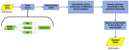
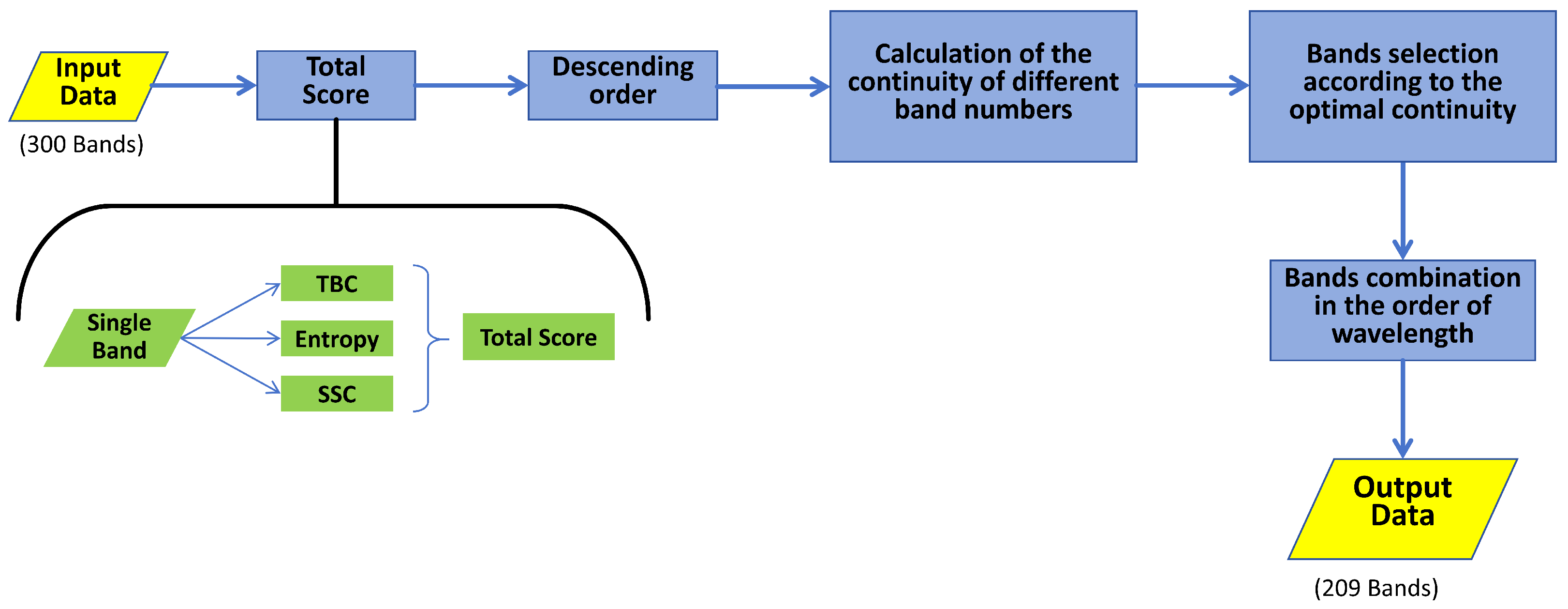
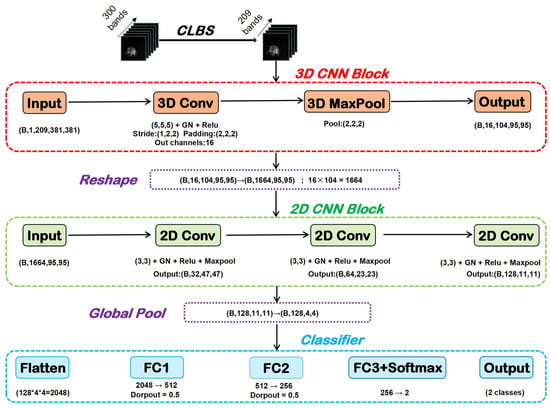
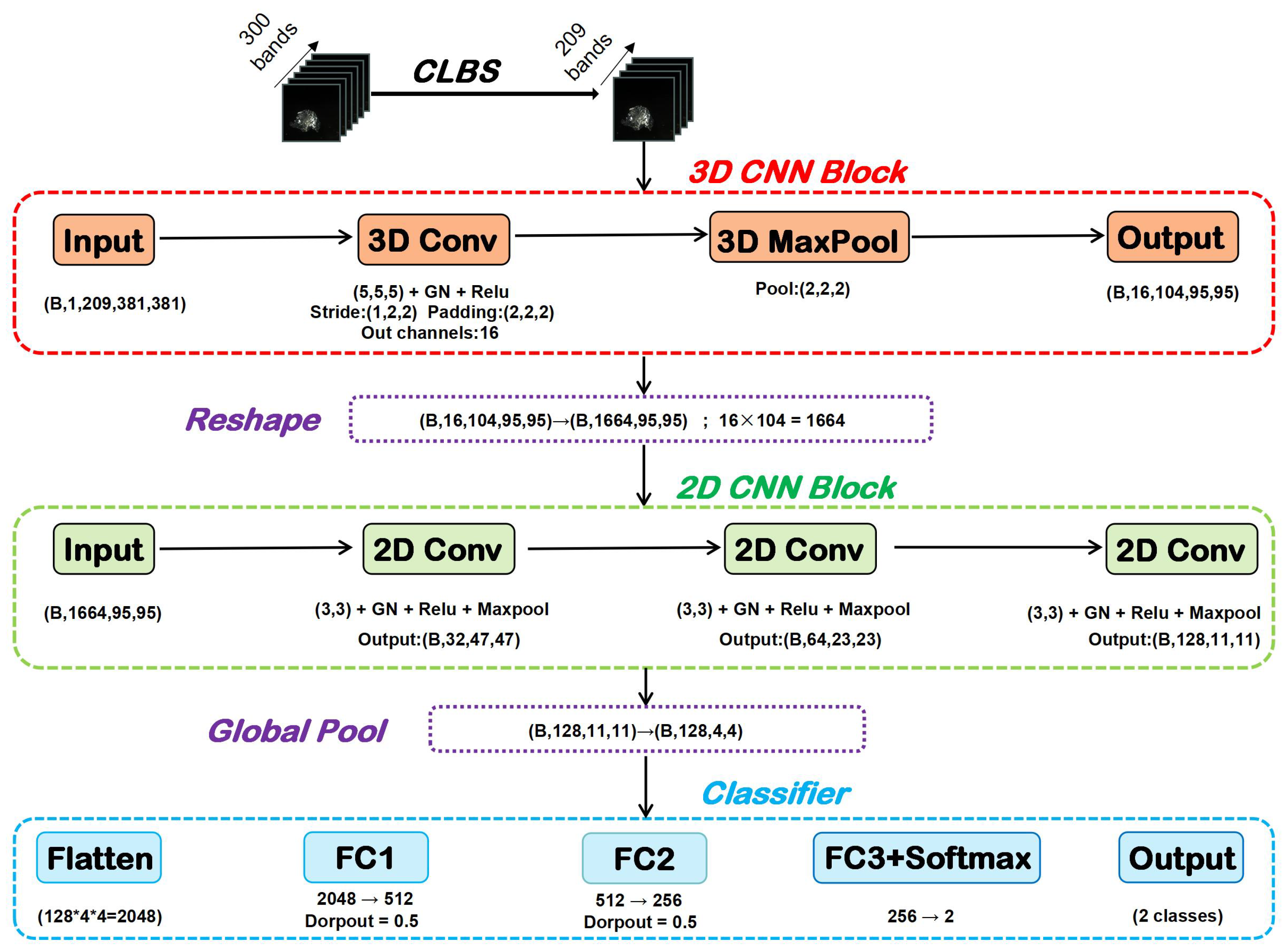
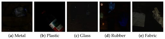
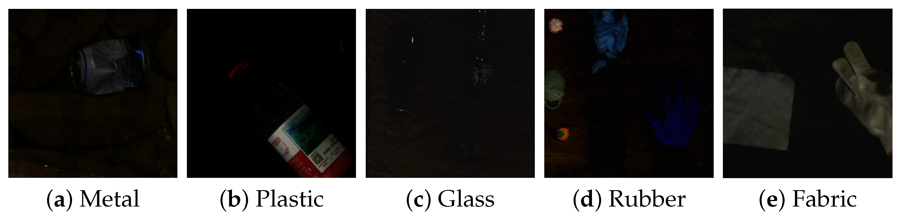
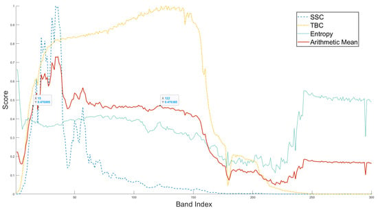
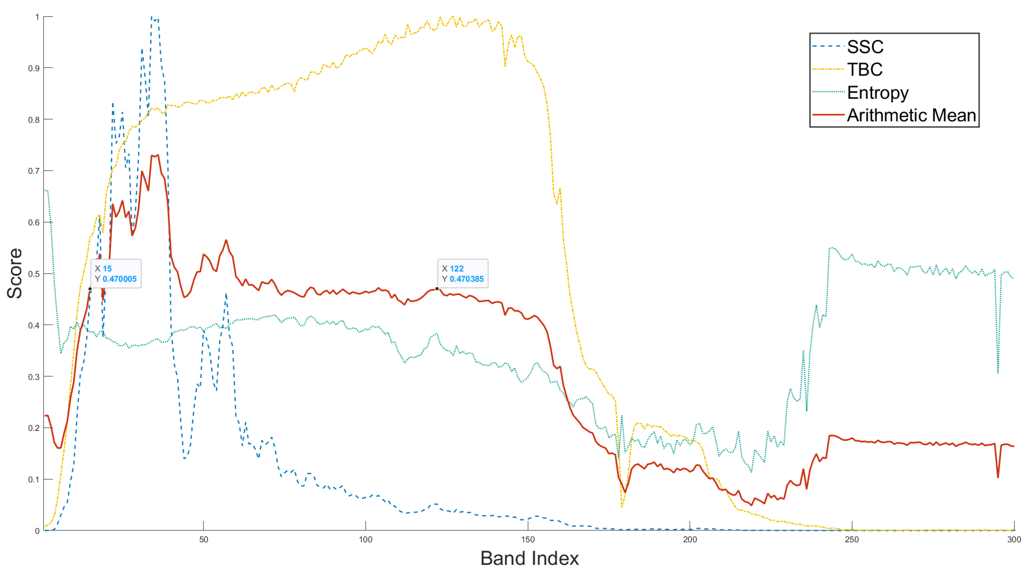
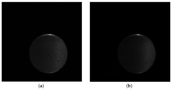
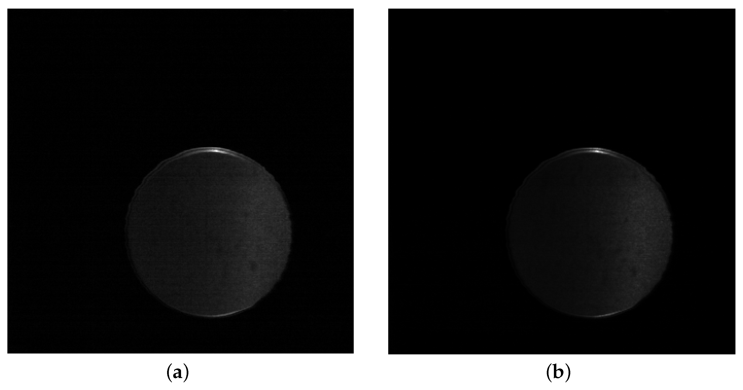
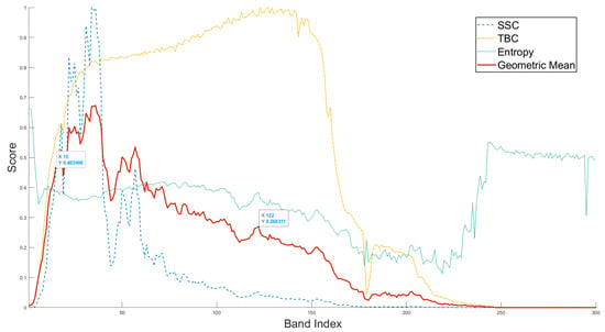
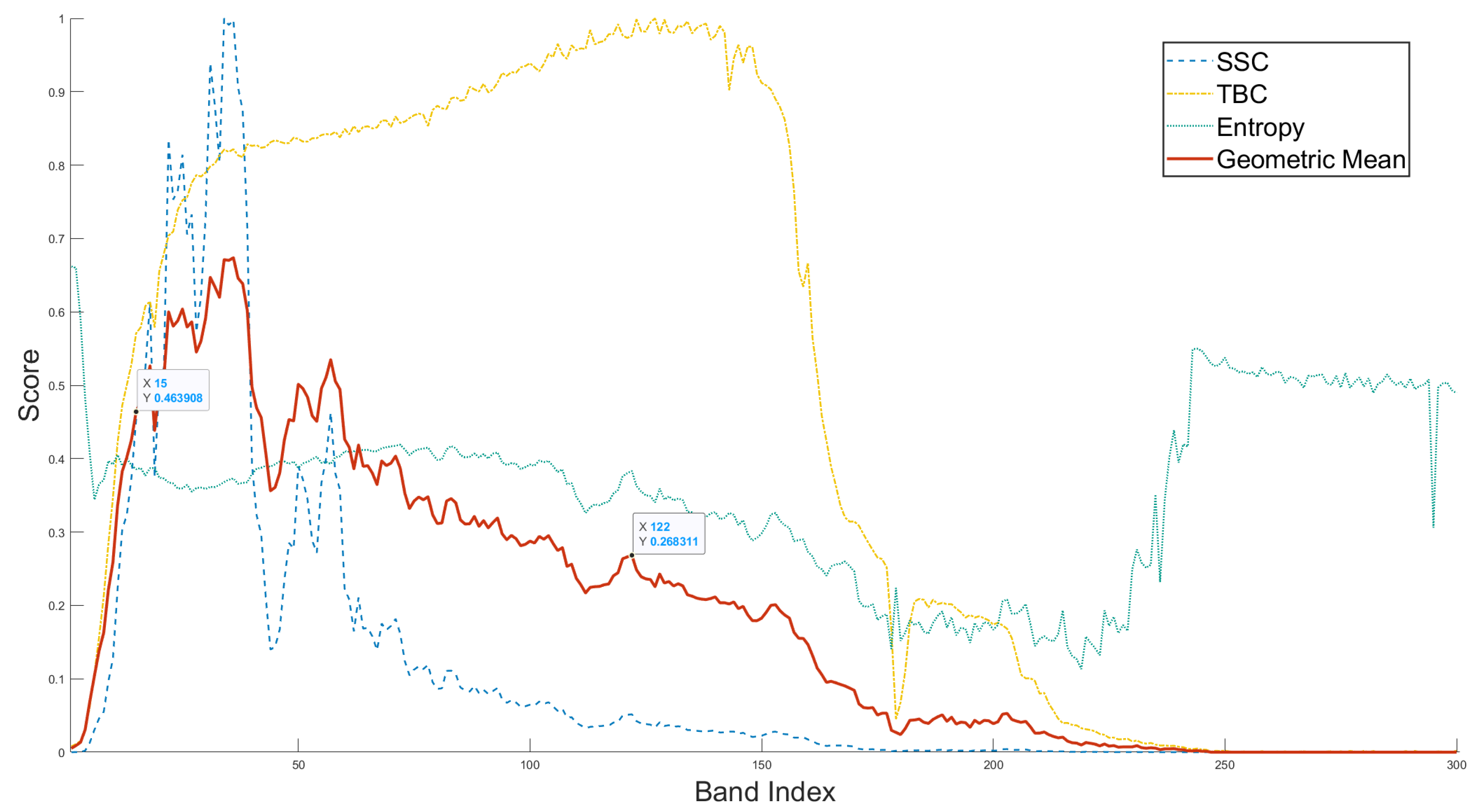
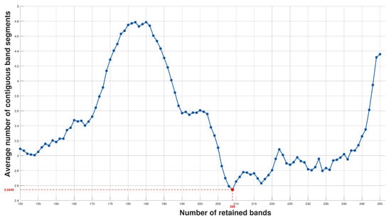
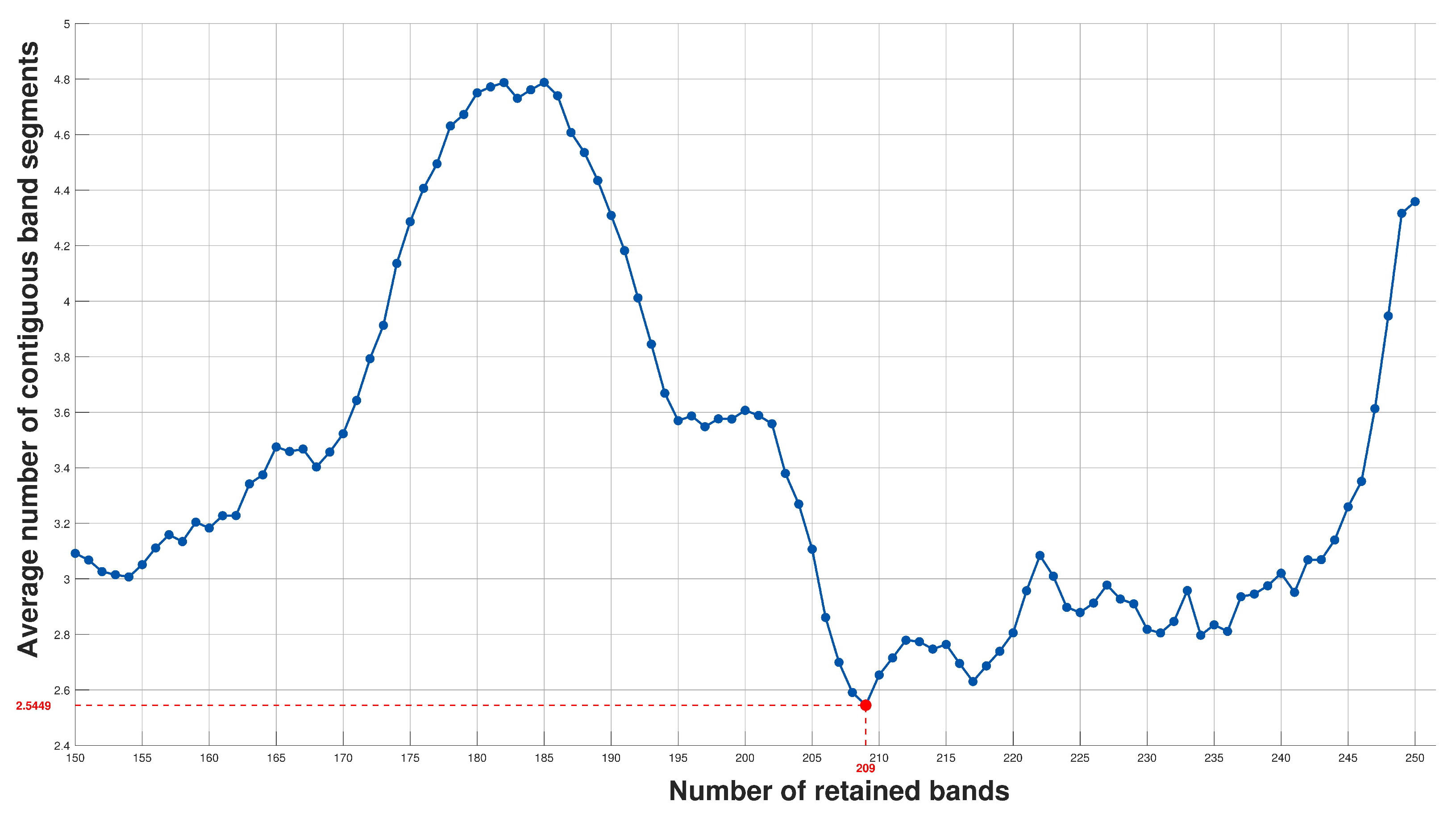
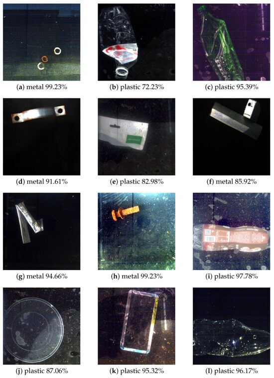
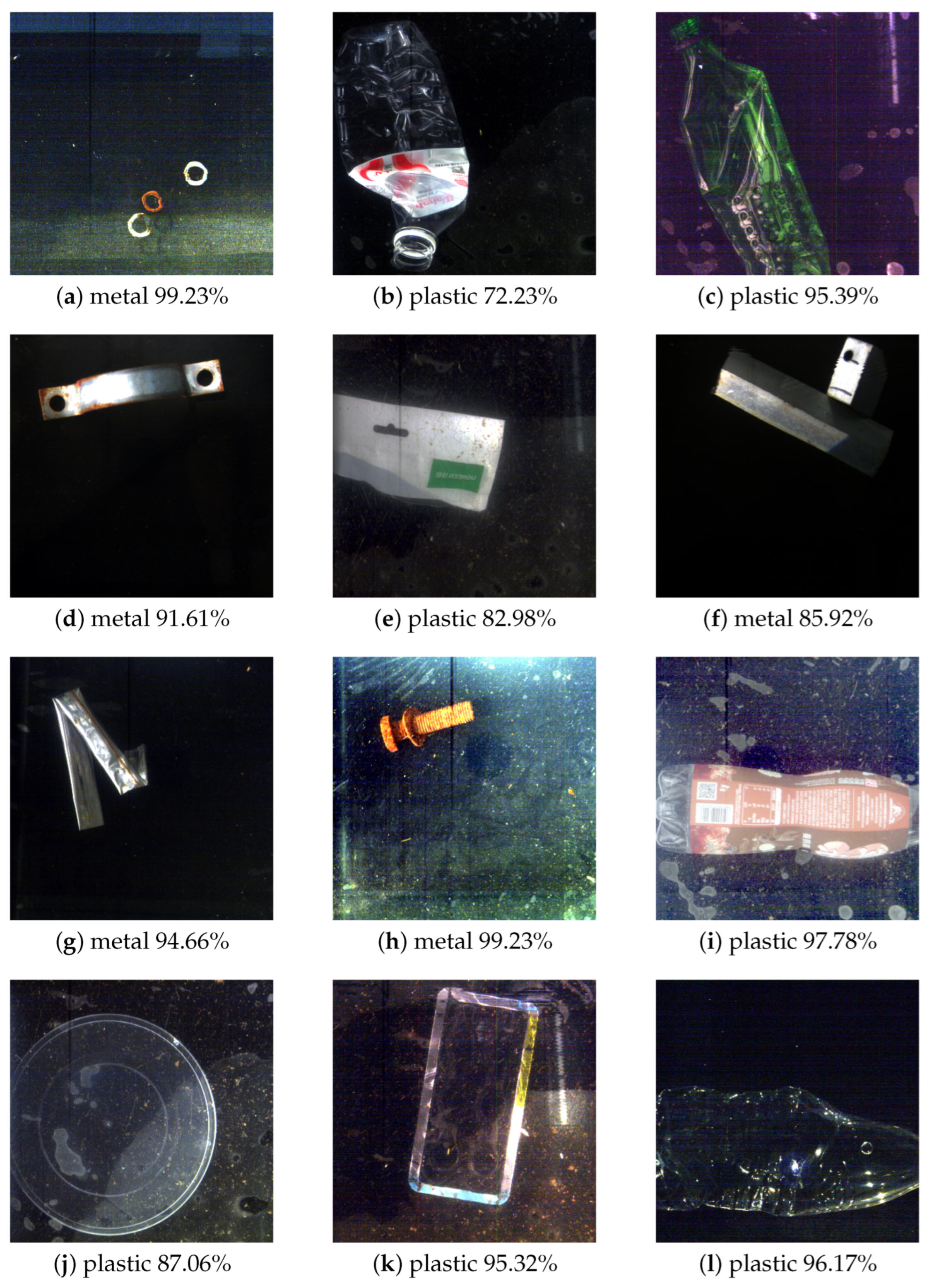

Disclaimer/Publisher’s Note: The statements, opinions and data contained in all publications are solely those of the individual author(s) and contributor(s) and not of MDPI and/or the editor(s). MDPI and/or the editor(s) disclaim responsibility for any injury to people or property resulting from any ideas, methods, instructions or products referred to in the content. |
© 2026 by the authors. Licensee MDPI, Basel, Switzerland. This article is an open access article distributed under the terms and conditions of the Creative Commons Attribution (CC BY) license.