IC-EWH: Energy-Weighted Hough Transform with Iterative Curvature Compensation for Squint Angle Estimation of Highly Squinted SAR

Highlights

What are the main findings?

• The integration of the energy-weighted Hough transform with adaptive scatterer screening yields robust envelope slope estimates.
• A closed-loop iterative curvature compensation strategy effectively suppresses the nonlinear envelope bending in highly squinted SAR, enabling reliable trajectory linearization for subsequent line detection.

What are the implications of the main findings?

• The method works reliably without ambiguous integer Doppler search, even when prior information is limited.
• Superior focusing and parameter accuracy on both simulated and real airborne data confirm its engineering value.

Abstract

Accurate estimation of the Doppler centroid is a prerequisite for achieving high-quality Synthetic Aperture Radar imaging. In highly squinted working scenarios, traditional frequency-domain methods depend on antenna pattern fitting. They are easily affected by pattern mismatch and strong scatterer interference. In addition, these methods cannot directly determine the Doppler ambiguity number. The range envelope-based Hough transform can correct linear range walk. It further realizes Doppler centroid estimation without ambiguity. However, range curvature hinders its estimation accuracy. To solve the above problem, this paper proposes a novel squint angle estimation scheme. The scheme organically combines closed-loop iterative range curvature compensation and energy-weighted Hough transform. Within a closed-loop iterative architecture comprising curvature compensation, line feature extraction, direction measurement, and angle refinement, the presented method progressively rectifies curved trajectories, yields robust squint angle estimates, and further derives the unambiguous Doppler centroid indirectly. Both simulated datasets and real airborne SAR measurements demonstrate the effectiveness and robustness of the proposed method.

1. Introduction

Synthetic Aperture Radar (SAR), as an all-time, all-weather active microwave remote sensing tool, plays an important role in fields such as military reconnaissance, topographic mapping, and disaster monitoring. The continuous pursuit of higher resolution and flexible observation modes imposes severe constraints on system stability, data throughput, and complex signal processing [1]. With the continuous expansion of SAR system operating modes, high-squint SAR has become a research hotspot in recent years due to its more flexible observation geometry and longer pre-warning time [2]. However, under the high-squint mode, the relative motion between the radar platform and the target is significant, leading to pronounced two-dimensional coupling and range curvature in the echo signals [3]. To address these issues, many scholars have dedicated themselves to the improvement of high-squint imaging algorithms. Xiong et al. [4] proposed an improved Omega-K algorithm using squint-equivalent wavelength, which effectively overcomes errors in the derivation of the 2D spectrum under complex geometry; Guo et al. [5] proposed a modified range–Doppler algorithm that effectively decouples and compensates for residual phases through nonlinear chirp scaling; Guo et al. [6] proposed an Extended Polar Format Algorithm (EPFA) for high-resolution scenes to eliminate wavefront curvature errors; for the more complex high-squint sliding spotlight mode, Liu et al. [7] proposed a fine focusing strategy combining range walk correction and an improved range migration algorithm. While autofocus methods such as [8] address azimuth spatial-variant errors, their performance remains sensitive to the initial parameter accuracy. Besides continuously improving the imaging algorithms themselves, obtaining accurate Doppler parameters is equally important; precise estimation of the squint angle or Doppler parameters is a prerequisite for achieving high-quality high-squint SAR imaging [9].

Classical frequency-domain parameter estimation methods mainly rely on the phase or amplitude spectrum information of the echo. In terms of phase-based estimation, Doppler centroid estimation based on frequency-domain cross-correlation [10,11,12,13], phase-based joint Doppler estimation [14,15,16], and phase parameter estimation for complex targets [17] have been widely applied. These types of algorithms extract Doppler parameters with high precision by calculating the phase difference between adjacent azimuth samples or adjacent looks. In terms of amplitude-spectrum-based estimation, the conventional energy centroid method [18,19] attempts to perform Doppler centroid estimation by fitting the energy distribution of the antenna pattern. This method has high computational efficiency but imposes extremely strict requirements on scene uniformity. Cheng et al. [20] proposed an improved adaptive Doppler centroid estimator that maintains spectral symmetry by adaptively adjusting the center and bandwidth of the weighting function, effectively eliminating the estimation bias of traditional methods. These frequency-domain methods generally achieve high estimation accuracy under low- to medium-squint angles or when a good initial value is available. However, frequency-domain estimation methods based on antenna pattern fitting are severely affected by sampling ambiguity, pattern errors, and strong point scatterer interference, and they are hard to directly resolve the Doppler ambiguity number. Under high-squint observation conditions, this limitation is significantly amplified. In such cases, the true Doppler centroid frequency often far exceeds the pulse repetition frequency (PRF), resulting in severe integer Doppler ambiguity. As ambiguity number is hard to be directly solved, frequency-domain methods often need to search and match ambiguity parameters during baseband estimation. This tends to considerably expand the parameter search space, and the estimation easily falls into a local optimum and model mismatch under low signal-to-noise ratio (SNR), strong clutter and complex scene conditions.

To circumvent the inherent ambiguity problems in the phase and frequency domains, some researchers have turned their attention to the geometric data domain, attempting to perform parameter estimation using the echo envelope trajectories of targets. The Hough transform, as a classical line detection tool, has also been widely applied in SAR trajectory extraction, parameter estimation, and linear target detection such as ships due to its strong noise robustness and global spatial search capability [21,22,23]. Skingley et al. [24] introduced the conventional Hough transform into SAR processing, achieving line detection by mapping the image space to the parameter space. However, this method is highly sensitive to trajectory curvature, and its accumulation performance degrades significantly when the envelope nonlinearity is strong. For distributed targets like ships, echo coupling among multiple scatterers, together with ship roll–pitch–yaw-induced phase modulation and envelope distortion, further deteriorates the line detection performance of the traditional Hough transform. Barbarossa [25] proposed the combined Wigner–Hough transform (WHT) method, enabling effective analysis of multi-component linear frequency-modulated signals. On this basis, Jiao et al. [26] further proposed an improved WHT method that enhances parameter estimation accuracy through local peak extraction combined with time-frequency analysis, although it still suffers from cross-term interference under low SNR. The aforementioned WHT and its derivatives were originally designed for ground moving targets. However, the severe range walk and Doppler centroid shift caused by unknown radial velocities of moving targets are geometrically similar to the echo trajectories observed in high-squint static-target scenarios. As pointed out in a recent study by Wang et al. [27], both high squint angles and unknown target motion parameters can induce severe nonlinear envelope curvature and Doppler centroid ambiguity in the range-azimuth domain. Therefore, such moving-target-based parameter estimation algorithms can also be used for comparison and reference in high-squint scenarios under certain conditions. Zhang et al. [28] proposed a hierarchical statistical detection method for targets in SAR images based on the discrete Hough transform. However, most existing geometric-domain detection methods based on the Hough transform are built on the premise that “target trajectories can be approximated as straight lines.” Under high-squint conditions, the cross-range cell phenomenon is extremely severe, and target envelope trajectories often exhibit pronounced nonlinear curvature characteristics. Directly applying global straight-line searching to uncompensated data will cause insufficient energy accumulation due to trajectory curvature, resulting in mainlobe broadening, parameter deviation and false peaks [29]. To address such nonlinear envelope curvature, Gu et al. [30] proposed a hyperbolic range model for high-squint scenarios. However, such high-precision nonlinear geometric models often involve complex coupling of higher-order terms. When incorporating such nonlinear models into existing Hough transform-based trajectory detection frameworks for squint angle search and estimation, extremely difficult parameter space mapping problems arise. On the other hand, Song et al. [31] pointed out that directly applying conventional multi-dimensional parameter optimization algorithms to solve such complex nonlinear target models not only incurs heavy computational burdens but also makes algorithm performance highly sensitive to initial parameter settings and prone to falling into local optima. It is a key challenge to maintain the noise robustness of the Hough transform while suppressing nonlinear curvature interference. This problem limits the parameter estimation accuracy of geometric methods in highly squinted SAR and needs further improvement.

To address the above issues, this paper proposes a novel squint angle estimation scheme that synergistically combines closed-loop iterative range curvature compensation with an energy-weighted Hough transform (IC-EWH). This algorithm estimates the Doppler centroid by exploiting the intrinsic relationship between the slope of the echo envelope and the squint angle. It can obtain an absolute Doppler centroid estimation even under conditions of limited prior information about the squint angle, thereby avoiding the uncertainty associated with ambiguity number search in conventional frequency-domain methods. To mitigate the impact of envelope curvature on estimation accuracy, an iterative estimation framework consisting of “curvature compensation, line extraction, direction detection, and angle update” is designed. By leveraging the intrinsic relationship between envelope curvature and the squint angle, the influence of envelope curvature is gradually eliminated during the iteration process, ensuring high-precision estimation performance. To comprehensively validate the effectiveness of IC-EWH, this paper designs ideal point-target simulations, a ship-target cluster simulation, and an airborne real-data experiment. The point-target simulation evaluates the theoretical accuracy and convergence characteristics of the algorithm, the ship-target simulation examines its adaptability in complex distributed target scenarios, and the real-data experiment tests its engineering usability in practical environments. Compared with standard Radon/Hough techniques that assume linear trajectories or fit explicit nonlinear curves, IC-EWH iteratively linearizes the envelope and adopts a simple linear Hough transform to avoid complicated parameter-space mapping. Energy-weighted voting combined with adaptive scatterer screening further suppresses clutter and concentrates voting accumulation on real target scatterers.

The main contributions of this paper are as follows:

1. An iterative range curvature compensation strategy in the range-azimuth envelope domain is proposed. This strategy constructs a range curvature compensation term using the current squint angle estimate and gradually reduces the quadratic curvature component in the target trajectory through inverse interpolation resampling, thereby providing a more stable geometric structure foundation for subsequent structural detection.

2. An envelope direction estimation method combining adaptive scatterer screening and an energy-weighted Hough transform is proposed. Adaptive threshold screening and local density constraints are employed to extract effective scattering structures, and the amplitudes of scatterers are used as voting weights in the Hough transform. This approach concentrates the voting energy for envelope direction estimation and reduces the influence of isolated noise points and clutter-induced false peaks on angle estimation.

3. A closed-loop iterative convergence determination mechanism based on a sliding window mean is constructed. This mechanism evaluates iteration stability using the mean value of multiple estimation results. It can suppress local fluctuations caused by noise perturbations, multi-target coupling, and discrete sampling errors, thereby improving the robustness of the final squint angle estimation.

2. Squinted SAR Imaging Geometry and Parameter Estimation Accuracy Requirements

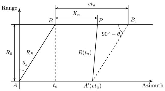
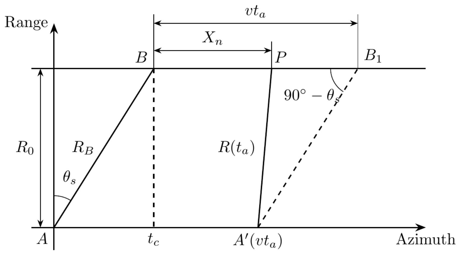
The geometric relationship of a squinted SAR operation is shown in Figure 1. The radar platform flies in a straight line along the flight path at a constant velocity v, with the flight path direction corresponding to the azimuth direction. When the beam line-of-sight deviates from the broadside direction, the system operates in squinted mode. The angle between the beam center line and the broadside direction is defined as the squint angle ${\theta }_s$. When the beam points forward, ${\theta }_s>0$; when pointing backward, ${\theta }_s<0$. In forward squint mode, the Doppler centroid frequency is positive, and the instantaneous slant range decreases as the platform advances.

Figure 1. Geometric model of squinted SAR imaging.

Let the time when the aircraft is at point A be the azimuth slow time zero ($t_a=0$). At this moment, the beam center passes through point B, and the distance from the radar to point B is defined as the reference slant range $R_B$. The lateral distance between point target P and point B along the line parallel to the flight path is denoted as $X_n$. After time $t_a$, the aircraft flies to point $A^{\prime }$, moving a distance $v{t}_a$ along the flight path.In triangle $P{A}^{\prime }{B}_1$, the instantaneous slant range from the radar to point target P can be obtained using the law of cosines:

$$R\left(t_a\right)=\sqrt{R_B^2+{(v{t}_a-X_n)}^2-2R_B(v{t}_a-X_n)sin{\theta }_s}.$$

(1)

To separate the linear range walk and higher-order curvature, we expand $R\left(t_a\right)$ in a Taylor series around the beam-center crossing time $t_0=X_n/v$. Let $\tau =t_a-X_n/v$. Performing the expansion up to the third order yields

$$\begin{array}{cc}\hfill R\left(\tau \right)& =R_B-vsin{\theta }_s\tau +{\displaystyle \frac{v^2{cos}^2{\theta }_s}{2R_B}}{\tau }^2+{\displaystyle \frac{v^3{cos}^2{\theta }_{s}sin{\theta }_s}{2R_B^2}}{\tau }^3+R_4\left(\xi \right),\hfill \end{array}$$

(2)

where $R_4\left(\xi \right)$ stands for the Lagrange remainder of the fourth order.

For typical airborne highly squinted SAR parameters (v $\le 150$ m/s, $R_B\ge 3000$ m, ${\theta }_s\le {65}^{\circ }$ and a synthetic aperture time $T_a<3$ s), the magnitude of the third-order term can be bounded by

$$\left|{\displaystyle \frac{v^3{cos}^2{\theta }_{s}sin{\theta }_s}{2R_B^2}}{\left({\displaystyle \frac{T_a}{2}}\right)}^3\right|<0.02\mathrm{m}.$$

(3)

This value is at least one order of magnitude smaller than typical high-resolution range resolutions (>0.5 m), and the fourth-order remainder $R_4\left(\xi \right)$ is even smaller. Hence, for envelope-based processing aimed at estimating the squint angle, it is sufficient to retain only the constant, linear, and quadratic terms. Dropping the terms of order ${\tau }^3$ and higher leads to the simplified range model:

$$R\left(t_a\right)\approx R_B-vsin{\theta }_s\left(t_a-{\displaystyle \frac{X_n}{v}}\right)+{\displaystyle \frac{v^2{cos}^2{\theta }_s}{2R_B}}{\left(t_a-{\displaystyle \frac{X_n}{v}}\right)}^2.$$

(4)

All subsequent derivations that deal with the echo envelope and its slope/curvature will be based on this model. The neglected cubic and higher-order components are well below the range cell size and have negligible impact on the slope detection.

According to the Doppler effect,

$$f_d\left(t_a\right)=-{\displaystyle \frac{2}{\lambda }}{\displaystyle \frac{\mathrm{d}R\left(t_a\right)}{\mathrm{d}{t}_a}}.$$

(5)

where $\lambda$ is the radar operating wavelength. Taking the derivative of Equation (4) at $t_a={\displaystyle \frac{X_n}{v}}$, the relationship between the Doppler centroid frequency and the squint angle is obtained:

$$f_{dc}={\displaystyle \frac{2v}{\lambda }}sin{\theta }_s.$$

(6)

From Equation (6), it can be seen that $f_{dc}$ and ${\theta }_s$ have a one-to-one correspondence. If ${\theta }_s$ can be accurately estimated, the absolute Doppler centroid frequency can be directly calculated.

The squint angle ${\theta }_s$ and its corresponding absolute Doppler centroid frequency $f_{dc}$ are key parameters for ensuring effective focusing of high-squint SAR images. Taking the classic range–Doppler (RD) imaging algorithm as an example, assume the estimated Doppler centroid is ${\widehat{f}}_{dc}=f_{dc}+\Delta f_{dc}$, where $\Delta f_{dc}$ is the estimation error. This error, when introduced into the core processing steps of the RD algorithm, will degrade the final imaging quality.

The most direct effect of Doppler centroid estimation error is reflected in the range migration correction step, often leading to severe residual errors and two-dimensional defocusing. Under high-squint conditions, the range walk to be corrected corresponds to the first-order term of the slow time $t_a$ in Equation (4). Combined with Equation (6), the theoretical value of range walk is closely related to the Doppler centroid:

$$R_w\left(t_a\right)=vsin{\theta }_s{t}_a={\displaystyle \frac{\lambda f_{dc}}{2}}{t}_a.$$

(7)

If there is a Doppler centroid estimation error $\Delta f_{dc}$ in actual processing, the residual range walk over the entire synthetic aperture time $T_a$ is

$$\Delta R_w={\displaystyle \frac{\lambda }{2}}\Delta f_{dc}{T}_a.$$

(8)

If the condition $|\Delta R_w|\le {\rho }_r/2$ is met, the total residual range walk across the entire aperture stays within half a range cell. Consequently, the compressed envelope of a point target does not migrate into an adjacent range cell, and coherent azimuth integration remains undisturbed, which meets the basic requirements of envelope alignment. Substituting Equation (8) immediately yields the required Doppler centroid accuracy:

$$|\Delta f_{dc}|\le {\displaystyle \frac{{\rho }_r}{\lambda T_a}}.$$

(9)

In high-squint mode, $T_a$ is often large, so the accuracy requirement for $\Delta f_{dc}$ is also stricter. Taking the simulation parameters in this paper as an example: when ${\rho }_r=1.5\mathrm{m}$, $\lambda =0.03\mathrm{m}$, and $T_a\approx 2.67\mathrm{s}$, we have

$$|\Delta f_{dc}|\le {\displaystyle \frac{{\rho }_r}{\lambda T_a}}\approx {\displaystyle \frac{1.5}{0.03\times 2.67}}\approx 18.7\mathrm{Hz}.$$

Furthermore, Doppler centroid error also causes an azimuth position shift in the target. The azimuth compression step of the RD algorithm also depends on the Doppler centroid estimation. From the linear time-frequency relationship, a Doppler centroid error $\Delta f_{dc}$ effectively shifts the reference function in the azimuth frequency domain, which translates into a time delay in the time domain:

$$\Delta t_a=-{\displaystyle \frac{\Delta f_{dc}}{K_a}}.$$

(10)

where $K_a$ is the azimuth chirp rate, approximately expressed as

$$K_a\approx -{\displaystyle \frac{2v^2{cos}^3{\theta }_s}{\lambda R_B}}.$$

(11)

This time delay ultimately results in a geometric position shift in the target in the azimuth direction of the image:

$$\Delta X=v\Delta t_a={\displaystyle \frac{\lambda R_B}{2v{cos}^3{\theta }_s}}\Delta f_{dc}.$$

(12)

Under high-squint and long-range observation scenarios, since ${cos}^3{\theta }_s$ in the denominator is small, a small frequency-domain error $\Delta f_{dc}$ can be amplified, leading to significant geometric positioning errors. Taking the simulation parameters in this paper as an example: $v=150\mathrm{m}/\mathrm{s}$, $\lambda =0.03\mathrm{m}$, $R_B=3000\mathrm{m}$, ${\theta }_s={50}^{\circ }$. Substituting into Equation (12) yields the proportionality factor

$${\displaystyle \frac{\lambda R_B}{2v{cos}^3{\theta }_s}}\approx {\displaystyle \frac{0.03\times 3000}{2\times 150\times {0.6428}^3}}\approx 1.13\mathrm{m}/\mathrm{Hz}.$$

If the Doppler centroid estimation error $\Delta f_{dc}=18.7\mathrm{Hz}$, the azimuth shift $\Delta X\approx 1.13\times 18.7\approx 21.1\mathrm{m}$; under more extreme squint angles or longer ranges, the shift can increase to hundreds of meters or even kilometers.

In addition, parameter mismatch can also cause the azimuth processing band to deviate from the antenna mainlobe energy region, leading to effective spectrum truncation, which in turn causes a sharp drop in signal-to-noise ratio, degradation of azimuth resolution, and asymmetric sidelobe distortion. Given the severe impact of Doppler parameter errors on imaging quality, high-precision acquisition of the squint angle is crucial. However, under high-squint and complex clutter scenarios, existing parameter estimation algorithms still face several issues: conventional frequency-domain methods are prone to falling into the Doppler ambiguity blind zone and struggle to handle the strong two-dimensional coupling introduced by high squint; meanwhile, geometric feature extraction methods have difficulty overcoming the geometric model mismatch caused by high-order range curvature, and the robustness and estimation accuracy of current algorithms still have room for improvement.

3. The Proposed IC-EWH Method

IC-EWH takes range-compressed echo data as input. The initial squint angle estimate is denoted as ${\theta }_{\mathrm{init}}$, which can be set to $0^{\circ }$ or a coarse value provided by system parameters. The algorithm gradually approaches the true squint angle through a closed-loop iterative framework consisting of curvature compensation, structure extraction, direction detection, and angle update.

3.1. Range Curvature Compensation and Angle-Weighted Hough Detection

Let the range-compressed input be $I(r,a)$, where r and a are the range and azimuth indices, respectively. In this paper, the range index $r=1$ corresponds to the nearest slant range, with larger indices indicating increasing slant range; the azimuth index $a=1$ corresponds to the start of azimuth slow time, with larger indices indicating increasing azimuth slow time. In the displayed image, the horizontal axis represents range and the vertical axis represents azimuth. Let the platform velocity, scene center slant range, range sampling rate, pulse repetition frequency, speed of light, and azimuth slow time be denoted as v, $R_B$, $F_s$, $\mathrm{PRF}$, C, and $t_a$, respectively.

As shown in Section 2, the cubic and higher-order terms in the range model are well below one range cell for typical geometries, so the second-order approximation Equation (4) is sufficient for envelope curvature compensation. In the n-th iteration, based on the slant range model shown in Equation (4), the first-order coefficient corresponds to the Doppler centroid, and the second-order coefficient corresponds to the Doppler chirp rate. Since the first-order term (range walk) determines the envelope slope that is used to estimate the squint angle, it is deliberately preserved in the range-compressed envelope rather than being removed beforehand. Only the second- and higher-order curvature terms, which cause the nonlinear bending of the envelope, need to be compensated during the iterative process.

Taking the scene center reference point $X_n=0$ as an example, the range curvature to be compensated is defined as

$$R_c^{\left(n\right)}\left(t_a\right)={\displaystyle \frac{v^2{cos}^2{\theta }_s^{\left(n\right)}}{2R_B}}{t}_a^2,$$

(13)

where $R_c^{\left(n\right)}\left(t_a\right)$ represents the parabolic envelope curvature induced by the squinted geometry. This is then converted into pixel offset

$$\Delta r^{\left(n\right)}\left(t_a\right)=R_c^{\left(n\right)}\left(t_a\right){\displaystyle \frac{2F_s}{C}}.$$

(14)

Resampling is performed on the normalized magnitude image $A(r,a)$:

$$A_c^{\left(n\right)}(r,a)=A(r+\Delta r^{\left(n\right)}\left(t_a\right),a),$$

(15)

i.e., linear interpolation is used to reduce the quadratic curvature component in the range-azimuth envelope, making the target energy trajectory approximately straight and providing a stable geometric foundation for subsequent direction detection. When the resampling index falls outside the valid range $[1,N_r]$, the corresponding pixel is set to zero, ensuring that only physically meaningful data contribute to the subsequent Hough detection.

Subsequently, effective structural points are extracted from the compensated image. $A_c^{\left(n\right)}$ is normalized to $[0,1]$, and the $80\%$ quantile of the amplitude is taken as the adaptive threshold, constrained to the range $[0.2,0.8]$. For the initial mask obtained by threshold segmentation, refinement is performed using local density filtering (window $9\times 9$, effective point ratio threshold $0.18$) and minimum connected area constraint (50 pixels) to suppress isolated noise and weak clutter points. The normalized amplitudes of the extracted effective structural points are retained for energy weighting in the subsequent Hough voting stage.

For a candidate angle $\varphi$, all effective structural points are projected onto the $\rho$ axis according to the normal distance $\rho =acos\varphi +rsin\varphi$. Let $L_{\varphi }\left(q\right)$ be the sum of amplitudes of effective points projected into the q-th $\rho$ bin. To reduce discretization error, $L_{\varphi }\left(q\right)$ is smoothed with a window length of 3 to obtain ${\tilde{L}}_{\varphi }\left(q\right)$. The angle response function is further defined as

$$H\left(\varphi \right)=\sum _q{\left[{\tilde{L}}_{\varphi }\left(q\right)\right]}^2.$$

(16)

The sum of squares is chosen as the response metric because when effective points form a prominent linear structure along direction $\varphi$, the voting energy is concentrated in a few $\rho$ bins, resulting in a large sum of squares; if the points are randomly distributed, the energy is evenly dispersed, resulting in a small sum of squares. Compared with the maximum value metric, the sum of squares considers the contributions of all $\rho$ bins comprehensively and is more robust to multi-peak distributions.

The $\varphi$ corresponding to the peak of the angle response function is the Hough detection angle of the current iteration. This method focuses on the direction of the echo envelope rather than the specific line position; therefore, the voting distribution in the $\rho$ dimension is used only as an intermediate quantity, and the optimal $\rho$ does not need to be output.

In the above mechanism, amplitude information is used both for front-end effective point screening and as voting weights in Hough direction detection. By excluding noise points through adaptive thresholding and local density constraints, amplitude-weighted voting further enhances the response of the main structural direction while avoiding interference from weak clutter points on the voting results, thereby improving the robustness of the main direction estimation.

The curvature compensation in Equation (13) is formulated with the reference point $X_n=0$ at the scene center. For targets far away from the scene center, the actual range curvature may deviate from this nominal quadratic curve. Let $\Delta X$ denote the along-track offset. It can be demonstrated that the relative curvature difference is on the order of ${(\Delta X/R_B)}^2$. For typical airborne geometries with $R_B$ ranging from 3 to 10 km and a scene width smaller than 1 km, the resulting residual is far below one range resolution cell and exerts a negligible influence on the subsequent linear Hough detection. For very wide-swath spaceborne scenarios or extremely long integration times, range-dependent or block-wise compensation strategies can be readily embedded into the proposed iterative framework.

3.2. Relationship Between Echo Envelope Slope and Squint Angle

The Hough detection yields the direction of the echo envelope in the range-azimuth image. To obtain the squint angle estimate, further geometric conversion is required to calculate the squint angle from the echo envelope slope.

Let $\Delta r$ denote the pixel spacing in the range direction, corresponding to a physical slant range change in $C/\left(2F_s\right)$; let $\Delta a$ denote the pixel spacing in the azimuth direction, corresponding to a physical slow time change of $1/\mathrm{PRF}$. The pixel slope of the line in the image is defined as

$$k={\displaystyle \frac{\Delta r}{\Delta a}},$$

(17)

and this slope k satisfies the following relationship with the Hough normal angle ${\varphi }_H$:

$$k=cot{\varphi }_H.$$

(18)

Since the slant range interval corresponding to one pixel in the range direction is $C/\left(2F_s\right)$, and the slow time interval corresponding to one sampling interval in the azimuth direction is $1/\mathrm{PRF}$, the actual slant range change rate corresponding to the image slope k is

$${\displaystyle \frac{\mathrm{d}R}{\mathrm{d}{t}_a}}=k·{\displaystyle \frac{C/\left(2F_s\right)}{1/\mathrm{PRF}}}=k{\displaystyle \frac{C·\mathrm{PRF}}{2F_s}}.$$

(19)

This equation holds under the following premises: (i) k is the overall slope estimate of the envelope direction of effective points; (ii) in the range-compressed image, the slant range values of each pixel have been aligned with sub-pixel accuracy through interpolation resampling.

On the other hand, the first-order change rate of the target slant range with respect to azimuth slow time is obtained by differentiating Equation (4) with respect to $t_a$ and evaluating at $t_a=0$:

$${\displaystyle \frac{\mathrm{d}R}{\mathrm{d}{t}_a}}=-vsin{\theta }_s.$$

(20)

Combining Equation (19) and Equation (20), we obtain

$$k=-{\displaystyle \frac{2F_{s}v}{C·\mathrm{PRF}}}sin{\theta }_s.$$

(21)

This equation establishes the analytical relationship between the envelope slope k and the physical squint angle ${\theta }_s$. The expression for calculating the squint angle from the image slope is further obtained as

$${\theta }_s=arcsin\left(-{\displaystyle \frac{k·C·\mathrm{PRF}}{2F_{s}v}}\right).$$

(22)

In practical implementation, noise or clutter may cause the estimated slope k to yield an argument slightly outside the valid range $[-1,1]$ for the arcsine function. To ensure numerical stability, the argument is explicitly clipped to $[-1,1]$ prior to arcsine computation.

Therefore, in the n-th iteration, the envelope slope $k^{\left(n\right)}$ is obtained from the Hough detection angle ${\varphi }_H$, and then substituted into Equation (22) to obtain the new instantaneous squint angle estimate:

$${\theta }^{(n+1)}=arcsin\left(-{\displaystyle \frac{k^{\left(n\right)}·C·\mathrm{PRF}}{2F_{s}v}}\right).$$

(23)

In the presence of noise, the instantaneous slope estimate $k^{\left(n\right)}$ may fluctuate, leading to noisy angle estimates from Equation (23). This jitter is effectively suppressed by the sliding-window average described in Section 3.3, eliminating the need for explicit noise modeling within the Hough transform step.

Equation (21) is also used to define the Hough search angle range. Given the current squint angle search interval, the corresponding slope range is first calculated using Equation (21), and then mapped to the Hough normal angle range via Equation (18). This approach avoids blind search over the full angular domain, significantly reducing computational cost.

3.3. Closed-Loop Iteration and Convergence Judgment

After obtaining the new squint angle estimate, the next round of range curvature compensation directly uses the current single Hough detection result, thus forming a closed-loop iteration process of “range curvature compensation, structure extraction, weighted Hough detection, squint angle calculation, and re-compensation.” As the iteration proceeds, if the squint angle estimate gradually approaches the true value, the range curvature compensation constructed by Equation (13) becomes more accurate, the residual curvature in the compensated image decreases, and the main peak response in the Hough parameter space becomes more stable.

In real data processing, the single Hough detection angle may fluctuate slightly due to the influence of local strong scatterers, residual clutter, and multi-target coupling. If a certain instantaneous estimate is directly used as the final output, the result may not be sufficiently stable. Therefore, this paper applies a sliding window mean to the instantaneous squint angle estimates obtained from each iteration. When the number of iterations reaches the sliding window length W, the mean of the most recent W instantaneous estimates is calculated as

$${\overline{\theta }}^{\left(n\right)}={\displaystyle \frac{1}{W}}{\displaystyle \sum _{i=0}^{W-1}}{\theta }^{(n-i)}.$$

(24)

In this paper, $W=5$ is selected. If the change between two adjacent sliding window means satisfies

$$\left|{\overline{\theta }}^{\left(n\right)}-{\overline{\theta }}^{(n-1)}\right|<{\epsilon }_{\theta },$$

(25)

the estimation sequence is considered to have entered a stable state, and the iteration is terminated early. In this paper, the stability threshold is set to ${\epsilon }_{\theta }=0.{001}^{\circ }$.

It should be emphasized that the sliding window mean is used only for convergence judgment and final output; in each round of compensation update, the algorithm still uses the instantaneous estimate calculated from the current single Hough detection as the compensation angle for the next round. The sliding window mainly suppresses estimation oscillations and does not affect the iteration response speed. The final output squint angle is defined as the mean of the most recent W instantaneous estimates:

$${\theta }_{\mathrm{est}}={\displaystyle \frac{1}{W}}{\displaystyle \sum _{i=0}^{W-1}}{\theta }^{(N-i)},N\ge W.$$

(26)

When the actual number of iterations $N<W$, the final output angle is taken as the last instantaneous estimate. To prevent endless loops in extreme cases, a maximum number of iterations can be set, e.g., $N_{max}=50$. When this limit is reached, the iteration is forcibly terminated, and the final estimate is taken as the mean of the most recent W instantaneous estimates, accompanied by a warning flag.

In summary, the proposed method does not rely on a single Hough transform detection result. Instead, it enhances the linear structure of the target envelope through iterative range curvature compensation, obtains round-by-round angle estimates using energy-weighted Hough detection, and finally outputs the squint angle through a sliding window mean stability decision. This procedure effectively suppresses estimation fluctuations caused by noise, local strong scatterers, and multi-target coupling, thereby improving the stability of squint angle estimation in real data processing.

4. Experimental Results

To comprehensively verify the effectiveness and superiority of IC-EWH in squint angle and Doppler parameter estimation for high-squint SAR, this section designs and conducts point target simulation experiments, ship target group simulation experiments, and airborne real-data processing experiments. Regarding the selection of comparison algorithms for the real-data experiments, this paper selects four representative classical and improved algorithms, including the traditional energy centroid method and the improved energy centroid method in the frequency domain, the traditional Hough transform method in the spatial domain, and the improved Wigner–Hough transform method in the time-frequency domain, aiming to cover the core estimation strategies across different observation domains. In terms of evaluation metrics, since the simulation experiments possess ideal prior information, this paper directly employs parameter estimation error and convergence curves as direct evaluation metrics to verify the theoretical accuracy and robustness of IC-EWH under different signal-to-noise ratios, multi-target coupling conditions, etc. For the airborne real-data experiments, due to the complex actual motion state of the platform and the lack of absolute ground truth for squint angle and Doppler parameters, Nevertheless, the quality of the estimated parameters can be rigorously assessed through indirect means: residual Doppler analysis, global image quality metrics, and local focusing fidelity. A precise parameter estimate should minimize the residual Doppler centroid and produce the best 2D focusing quality; thus, these metrics collectively serve as surrogate fidelity indicators. Specifically, the parameters estimated by each algorithm are uniformly incorporated into the subsequent focusing process. By comparing the final residual Doppler characteristics, global image quality metrics, and average focusing quality metrics of strong scatterers, the parameter estimation accuracy of the algorithms in real complex scenarios is indirectly and quantitatively demonstrated.

4.1. Point Target Simulation and Algorithm Robustness Verification

This section verifies the algorithm performance through an airborne X-band high-squint SAR point target simulation experiment. The specific radar system and platform motion parameters are shown in Table 1. In the simulation scenario, five ideal point targets are arranged along the diagonal of the scene, as detailed in Table 2. To better reflect the physical characteristics of coexisting strong and weak scatterers in real complex scenarios, these five point targets are set with different backscattering amplitudes. Basic imaging tests are conducted for a squint angle of ${\theta }_{\mathrm{true}}={50.0}^{\circ }$, and the initial estimate is set to $0^{\circ }$ to verify the convergence capability of the algorithm under large initial prior deviation.

Table 1. Simulation parameters for high-squint SAR point targets.

Parameter	Symbol	Value
Carrier frequency	$F_c$	10 GHz
Platform velocity	v	150 m/s
Scene center reference slant range	$R_B$	3000 m
Platform height	H	1000 m
Signal bandwidth	$Bw$	100 MHz
Range sampling rate	$F_s$	200 MHz
Pulse repetition frequency	$\mathrm{PRF}$	4000 Hz
Pulse width	$T_r$	2 μs
True squint angle	${\theta }_{\mathrm{true}}$	${50.0}^{\circ }$

Table 2. Positions and amplitudes of the five simulated point targets.

Target	$\mathbf{\Delta }\mathit{x}$ (m)	$\mathbf{\Delta }\mathit{y}$ (m)	Normalized Amplitude
1	0	0	1.0
2	−6	−8	0.9
3	−3	−4	0.8
4	3	4	0.8
5	6	8	0.9

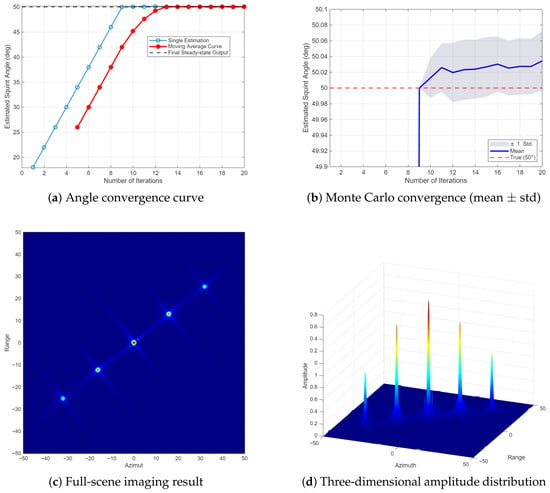
The experimental results are shown in Figure 2. From the single-realization convergence curve in Figure 2a, the sliding mean estimate converges smoothly after 12 iterations, with the final steady-state estimate being ${50.038}^{\circ }$, yielding an estimation error of only ${0.038}^{\circ }$ compared to the true squint angle. To assess the statistical stability, Figure 2b displays the mean convergence trajectory over 50 independent trials, with a shaded band representing $\pm 1$ standard deviation; the estimated band is mostly confined within $[{49.98}^{\circ },{50.08}^{\circ }]$, which demonstrates favorable statistical stability of the proposed algorithm. Subsequently, this high-precision squint angle estimate is fed into the Parametric Polar Grid Algorithm (PPGA), and the imaging results are shown in Figure 2c,d. From the two-dimensional full-scene result in Figure 2c, all five point targets distributed along the diagonal are well focused. Figure 2d presents the three-dimensional amplitude distribution of the scene. Despite the different backscattering amplitudes, each target exhibits a sharp impulse response with a highly concentrated mainlobe and symmetric sidelobes, free from noticeable defocusing or distortion.

Figure 2. Simulation experiment results.

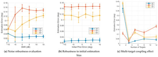
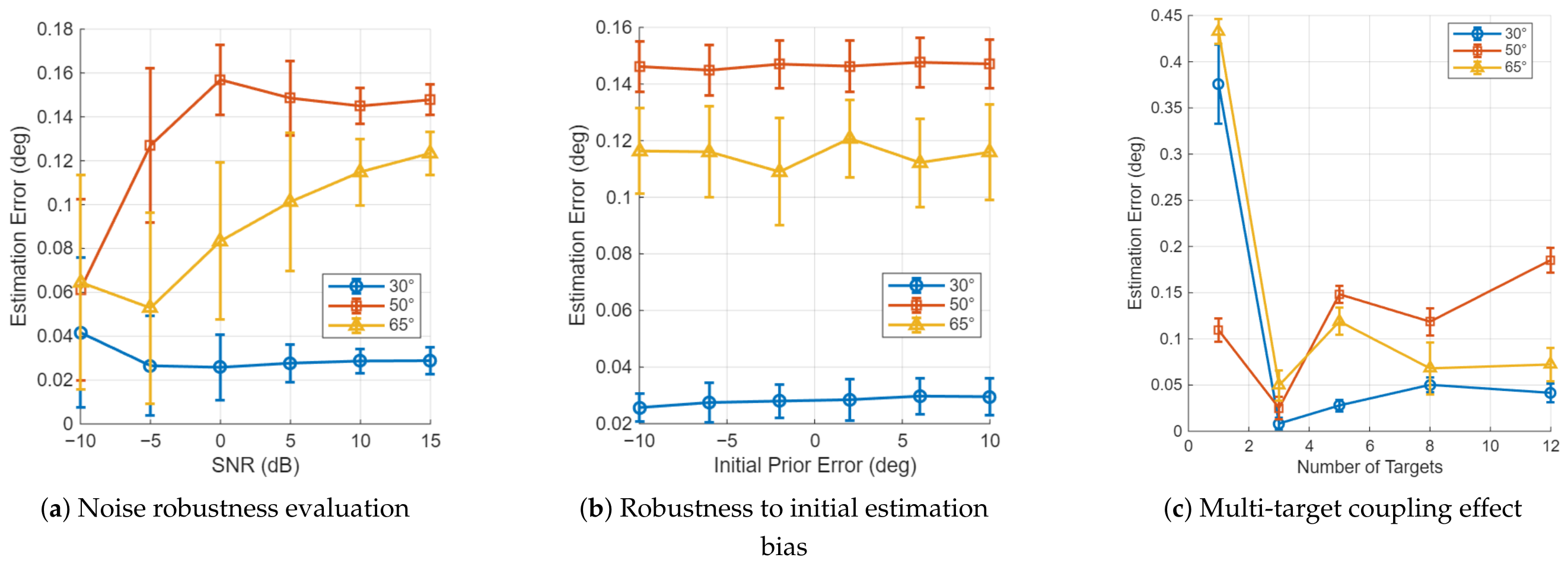
To further evaluate the robustness of the algorithm under different conditions, Monte Carlo experiments are conducted at three squint angles (${30}^{\circ }$, ${50}^{\circ }$, and ${65}^{\circ }$) from three aspects: signal-to-noise ratio, initial estimation bias, and number of targets in the scene. Under each parameter condition, 50 independent repetitions are performed, and the standard deviation of the estimation error is calculated. The experimental results are shown in Figure 3.

Figure 3. Estimation performance of IC-EWH in multi-dimensional robustness tests.

In the noise robustness test, the number of point targets is fixed at five, the initial estimation bias is set to ${10}^{\circ }$, and the signal-to-noise ratio varies from $-10\mathrm{dB}$ to $15\mathrm{dB}$. The statistical results are shown in Figure 3a. Under the three typical squint angles, the algorithm maintains small estimation errors under different SNR conditions. As the SNR increases, the estimation accuracy gradually improves. Under $-10$ dB SNR, the estimation error remains within an acceptable range across the three tested squint angles.

In the initial estimation bias robustness test, the SNR is fixed at $10\mathrm{dB}$, and the number of point targets is fixed at five. The initial estimation angle is set according to Equation (27):

$${\theta }_{\mathrm{init}}={\theta }_{\mathrm{true}}+\Delta {\theta }_{\mathrm{init}},$$

(27)

where $\Delta {\theta }_{\mathrm{init}}\in \{-{10}^{\circ },-6^{\circ },-2^{\circ },2^{\circ },6^{\circ },{10}^{\circ }\}$. The corresponding experimental results are shown in Figure 3b. Within the set initial bias range, the algorithm can gradually correct the estimate through iterative search and finally converge to near the true squint angle, indicating that IC-EWH does not have strict requirements on the initial estimate.

In the scene complexity test, the SNR is fixed at $10\mathrm{dB}$, the initial estimation bias is set to ${10}^{\circ }$, and the adaptability of the algorithm is examined by changing the number of point targets in the scene. The results are shown in Figure 3c. When the number of targets is small, there are insufficient effective points for Hough accumulation, and the estimation error is relatively large. As the number of targets increases, multi-target echoes provide richer spatial geometric constraints, and the estimation accuracy gradually improves. When the number of targets further increases, energy coupling between different echoes causes slight fluctuations in the error curve, but the overall estimation error remains at a low level, indicating that IC-EWH can adapt to multi-target scenarios.

In summary, the point target simulation verifies that IC-EWH can effectively converge and obtain accurate estimation results under different squint angles, different SNRs, different initial biases, and different numbers of targets, demonstrating the conceptual correctness and basic effectiveness of the method in ideal simulation environments.

4.2. Simulation Verification of Ship Target Group

To further verify the applicability of IC-EWH in complex distributed target scenarios, this subsection sets up a simulation scenario containing five ships. The five ships are located at the upper-left, upper-right, lower-left, lower-right, and center positions of the scene, respectively. Each ship is modeled as a distributed target consisting of multiple scatterers that form the hull outline, deck, and superstructures, with varying backscattering coefficients to emulate different ship types and sizes. The simulation parameters are consistent with those in Table 1, the initial estimated angle is still set to $0^{\circ }$, and ocean environment clutter is added to the echo with the signal-to-noise ratio set to $15\mathrm{dB}$.

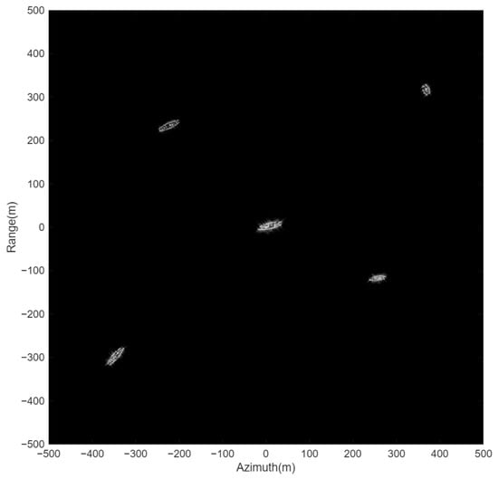
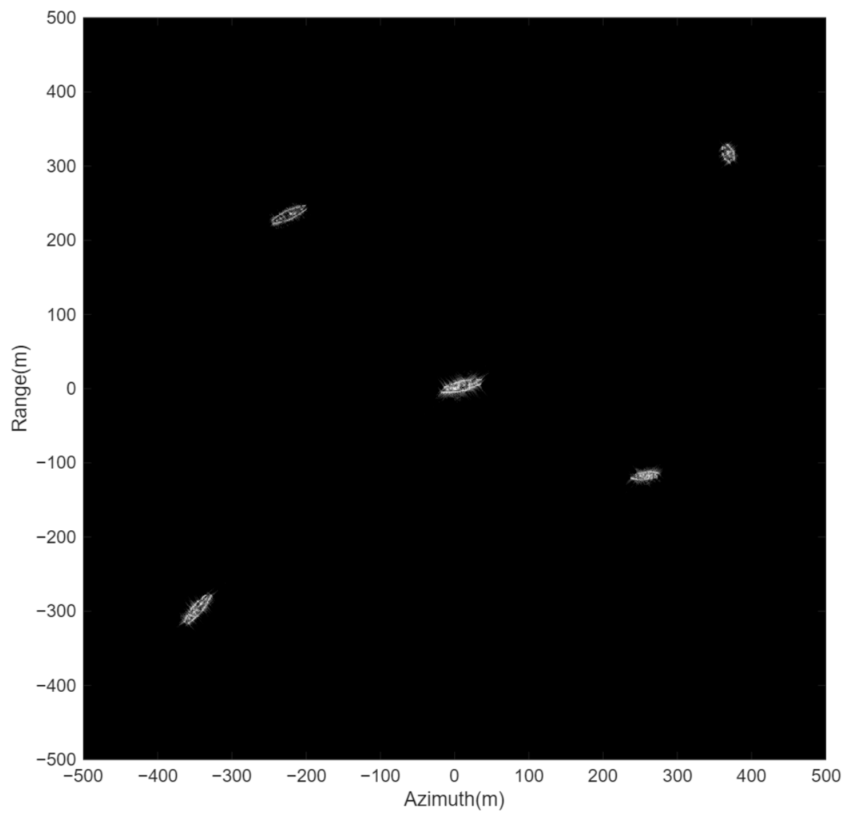
Figure 4 presents the final imaging results of the ship target group. The experiment converges after 18 iterations, yielding an output squint angle of ${49.84}^{\circ }$, with an error of only ${0.16}^{\circ }$ from the true value of ${50.0}^{\circ }$. In the imaging results, all five ships are clearly distinguishable, and their relative spatial positions are perfectly consistent with the preset coordinates in the simulation. The three scatterers within each ship are also well-focused, showing no obvious defocusing or geometric distortion, indicating that IC-EWH maintains high estimation accuracy when dealing with distributed multi-target scenarios.

Figure 4. Imaging results of ship target group simulation.

This simulation result further verifies the adaptability of the proposed method to complex target scenarios, complements the limitation of single ideal scatterers in point target simulation, and provides a more sufficient basis for subsequent real-data processing.

4.3. Real Data Experiment Verification

To verify the applicability of IC-EWH in actual airborne SAR data processing, real raw echo data are further used for experiments. For data reading, the range reading length is set to $N_r=4096$, and the azimuth reading length is fixed to $N_a$ = 16,384. In the experiment, relevant parameters are first read, and range compression is performed on the echo data. Then, the proposed method and four comparison methods are used to estimate the squint angle and Doppler centroid, and the estimation results are uniformly used for subsequent range migration correction, motion compensation, and PPGA focusing imaging.

The conventional Hough transform [24] and the proposed IC-EWH estimate the absolute squint angle directly from the geometric envelope without any prior; their estimated values are both around ${50}^{\circ }$. We therefore adopt ${50}^{\circ }$ as the nominal prior for the three methods that require it to resolve the PRF ambiguity: the conventional energy centroid [18], the improved energy centroid [20], and the improved Wigner–Hough transform [26]. Although IC-EWH does not require a prior, it is initialized at ${50}^{\circ }$ in this experiment solely to accelerate convergence. After 26 iterations, the focused imaging result of the real data is obtained, as shown in Figure 5.

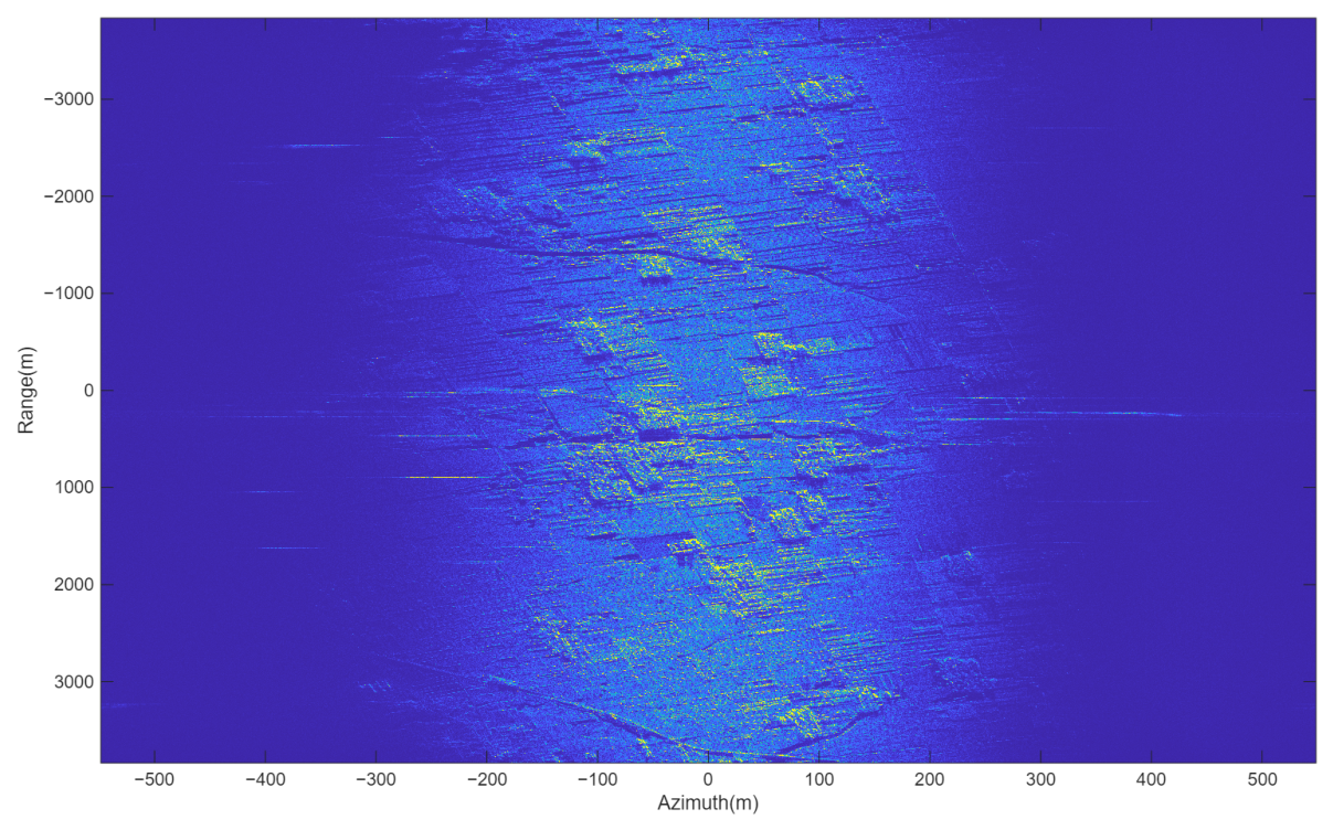
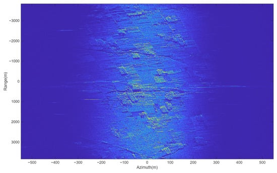
Figure 5. Focused imaging result of real data using IC-EWH.

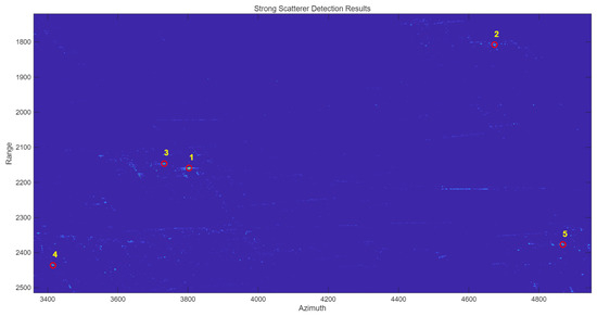
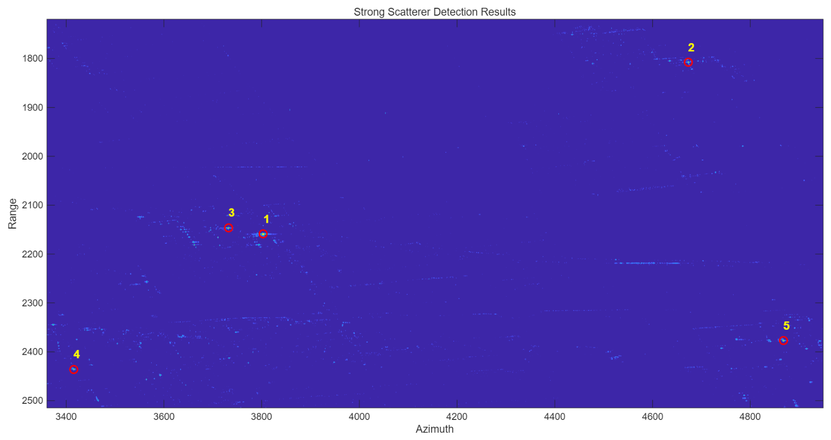
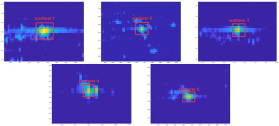
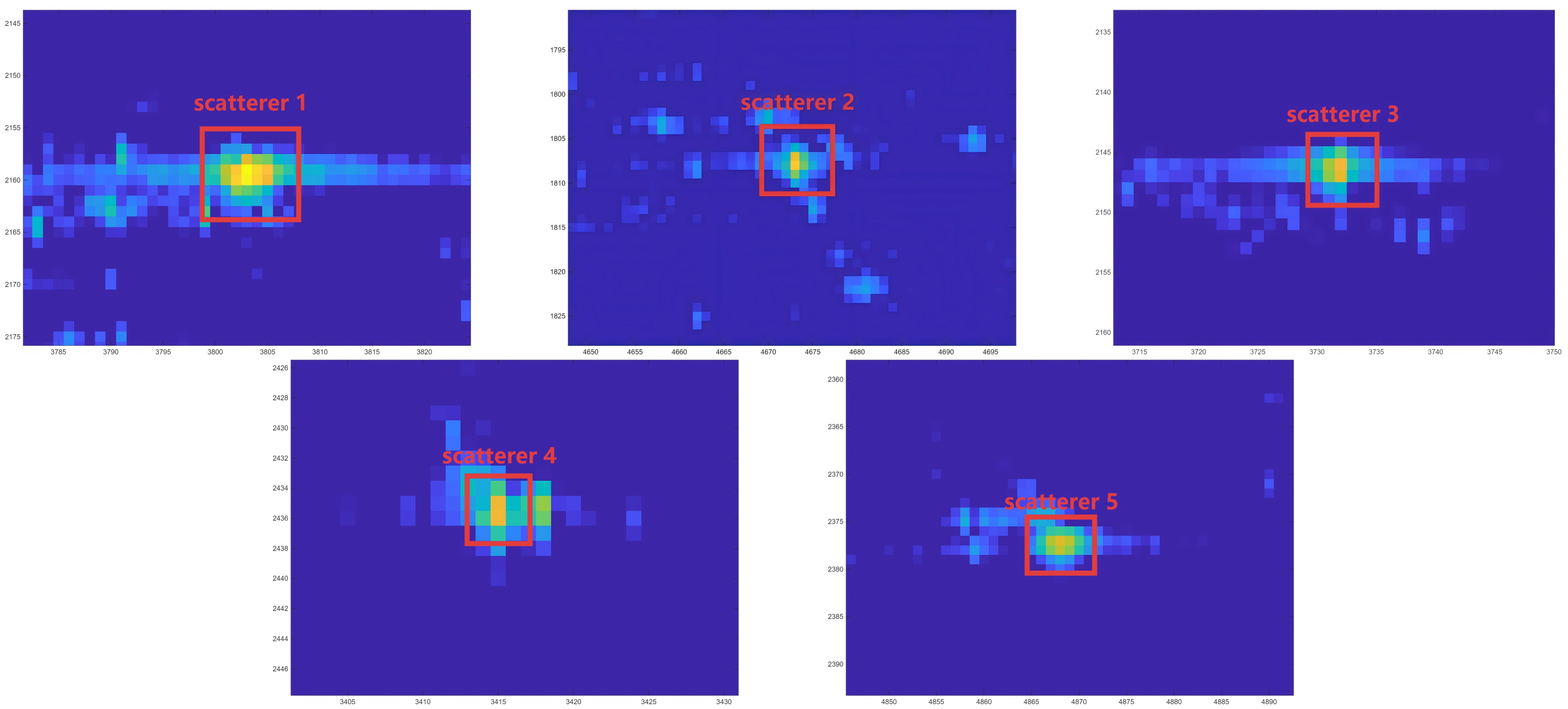
From Figure 5, it can be seen that after IC-EWH processing, the main ground object structures in the scene are effectively focused, with strong scatterers, edge contours, and local texture information being relatively clear, indicating that the proposed method can provide accurate parameter support for motion compensation and subsequent focusing imaging of actual airborne SAR data. To further observe the focusing details, five typical strong scatterers distributed in different areas are selected from the global imaging result for local magnification analysis. Their positions in the global image are shown in Figure 6, and the corresponding two-dimensional magnification results are shown in Figure 7. From the magnified images, although the targets exhibit some degree of azimuth sidelobe tailing due to the complex clutter background of the real environment and system non-ideal factors, the mainlobe energy of all five scatterers is highly concentrated, and the target mainlobes do not show asymmetric distortion or severe defocusing caused by Doppler parameter estimation errors. This further supports that IC-EWH can achieve high-precision parameter estimation, thereby ensuring excellent and robust imaging quality in complex real scenarios.

Figure 6. Detection results of strong scatterers. The numbered markers denote selected strong scatterers, where each number represents the sorted serial number of the corresponding scattering point ranked by peak energy.

Figure 7. Local magnification of strong scatterer focusing quality.

To further quantitatively evaluate the parameter estimation accuracy and imaging focusing quality of IC-EWH, the processing results of the five methods are compared. All methods use the same processing flow and system parameters, with only the squint angle and Doppler centroid estimation modules replaced. Therefore, the difference in final imaging quality directly reflects the performance of each parameter estimation method. The residual Doppler characteristics are calculated on the data after range migration correction and before PPGA imaging, and global image quality metrics such as image entropy, image contrast, image sharpness, and peak-to-mean ratio are calculated. The comparison results of the five methods are shown in Table 3.

Table 3. Comparison of residual Doppler centroid and global image quality metrics.

Metric	IC-EWH	Energy Centroid [18]	Improved Energy Centroid [20]	Conventional Hough [24]	Improved WHT [26]
Residual Doppler centroid/Hz	−0.0998	40.1364	10.8238	−3.9977	−57.6800
Doppler spectrum peak/Hz	−36.987	3.296	−24.358	−39.551	−92.896
Image entropy	18.9399	18.9296	18.9412	18.9433	18.9310
Image contrast	2.366	2.364	2.366	2.366	2.361
Image sharpness $\left(\times {10}^{-4}\right)$	7.452	7.160	6.940	6.982	9.589
Peak-to-mean ratio/dB	65.6479	64.4123	64.2545	65.0316	66.5070

To further analyze the focusing fidelity of local strong scattering centers, several point targets are selected from the imaging results, and the Peak Sidelobe Ratio (PSLR) and Integrated Sidelobe Ratio (ISLR) are calculated in their local neighborhoods. The average focusing quality metrics of strong scatterers for the five methods are shown in Table 4.

Table 4. Comparison of average focusing quality metrics for strong scatterers.

Metric	IC-EWH	Energy Centroid [18]	Improved Energy Centroid [20]	Conventional Hough [24]	Improved WHT [26]
2D PSLR/dB	−9.8300	−8.9904	−9.0028	−9.5468	−7.7602
2D ISLR/dB	−2.5216	−2.5649	−2.5408	−2.5342	−1.5251
Range PSLR/dB	−27.0299	−25.9717	−26.6385	−26.9873	−28.6572
Range ISLR/dB	−23.6297	−22.7956	−23.0707	−23.5391	−24.0164
Azimuth PSLR/dB	−16.3173	−15.6659	−15.7578	−16.0842	−12.6410
Azimuth ISLR/dB	−12.7182	−12.7551	−12.5807	−12.6793	−10.5559

Note: PSLR = Peak Sidelobe Ratio; ISLR = Integrated Sidelobe Ratio.

4.4. Ablation and Sensitivity Analysis

To further quantify the practical contribution of each algorithmic component, we conduct an ablation experiment on the airborne real dataset. Starting from the full IC-EWH pipeline, we disable one module at a time: curvature compensation, energy weighting, scatterer screening, and sliding-window averaging. Each variant is executed once, and the resulting squint angle estimate is used to perform range migration correction (RCMC). The residual Doppler centroid after RCMC serves as an indirect fidelity indicator: a smaller absolute residual indicates better envelope alignment and thus higher parameter accuracy. Table 5 summarizes the estimated angles, residual Doppler centroids, and runtimes.

Table 5. Ablation study on real data: estimated squint angle and residual Doppler after RCMC.

Method	Estimated Angle	Residual Doppler (Hz)	Time (s)
IC-EWH (full)	50.31°	−0.10	115.46
No curvature compensation	50.33°	−1.98	106.95
No energy weighting	50.37°	−6.21	116.61
No scatterer screening	50.27°	3.63	122.49
No sliding-window averaging	50.32°	−1.11	115.83

To evaluate the sensitivity of the adaptive threshold, we varied its percentile on the real dataset while keeping the density-filter parameters fixed at $9\times 9$ and the density ratio at $0.18$. The resulting residual Doppler centroid after RCMC was recorded.

As shown in Table 6, the residual Doppler centroid varies gradually from $-1.38$ Hz to $3.83$ Hz when the threshold percentile is swept from 70% to 90%. Of these, setting the threshold to 80% produces the minimal absolute residual and achieves a favorable tradeoff between clutter suppression and weak scatterer preservation. The residual remains at a low level with only mild fluctuation across the tested interval.

Table 6. Sensitivity of residual Doppler to the adaptive threshold percentile.

Percentile	Residual Doppler (Hz)	Absolute (Hz)
70%	−1.3847	1.3847
75%	−0.9157	0.9157
80%	−0.0998	0.0998
85%	0.2941	0.2941
90%	3.8295	3.8295

To evaluate the sensitivity of the density-filter parameters, we varied the window size and density ratio on the real dataset, while keeping the adaptive threshold fixed at 80%. The resulting residual Doppler centroid was recorded.

As Table 7 shows, the combination $(9\times 9,0.14)$ gives the smallest absolute residual Doppler, while all tested configurations yield comparable accuracy with variations within $0.1$ Hz.

Table 7. Sensitivity of residual Doppler to the density-filter parameters.

Window Size	Density Ratio	Residual Doppler (Hz)	Absolute (Hz)
$7\times 7$	0.14	0.0363	0.0363
$7\times 7$	0.18	0.0378	0.0378
$9\times 9$	0.14	0.0069	0.0069
$9\times 9$	0.18	−0.0998	0.0998
$11\times 11$	0.18	0.0305	0.0305
$11\times 11$	0.22	0.0924	0.0924

4.5. Computational Complexity Analysis

Table 8 reports the measured runtime and asymptotic complexity of the estimation component of each method. The measurements were obtained on a laptop PC equipped with a 13th Gen Intel Core i5-13420H processor operating at 2.10 GHz and 16 GB of RAM, using MATLAB R2025a. The real-data size is $N_r=4096$ and $N_a$ = 16,384.

Table 8. Runtime and complexity of the squint-angle/Doppler estimation methods.

Method	Runtime (s)	Asymptotic Complexity
Energy centroid [18]	0.6	$O(N_r{N}_{a}log{N}_a)$
Improved energy centroid [20]	0.7	$O(N_r{N}_{a}log{N}_a)$
Conventional Hough [24]	4.7	${O\left(N_{\theta }{N}_{\rho }\right) }^1$
Improved WHT [26]	0.8	${O(K{N}_{\mathrm{wvd}}{N}_{\mathrm{fft}}log{N}_{\mathrm{fft}}) }^2$
IC-EWH (proposed)	114.9 (4.42)	${O\left(I(N_r{N}_{a}log{N}_a+N_r{N}_a+N_{\mathrm{eff}}{N}_{\theta })\right) }^3$

Note: ¹ $N_{\theta }$: number of angle bins; $N_{\rho }$: number of $\rho$ bins. ² K: number of selected range bins; $N_{\mathrm{wvd}}$: WVD window length; $N_{\mathrm{fft}}$: FFT size. ³ I: number of iterations; $N_{\mathrm{eff}}$: number of effective points after screening.

In the conventional Hough transform, $N_{\theta }=3600$ (search range $[-{89.95}^{\circ },{89.95}^{\circ }]$, step $0.{05}^{\circ }$) and $N_{\rho }$ is automatically set by the built-in hough function, scaling with the image diagonal. For the improved WHT, $K\le 8$, $N_{\mathrm{wvd}}=512$, and $N_{\mathrm{fft}}=1024$. In the real-data experiment, the algorithm converged after $I=26$ iterations; $N_{\mathrm{eff}}$ is the count of effective points retained after adaptive screening, which is typically much smaller than the image size $N_r{N}_a$. IC-EWH incurs the highest total cost of $114.9$ s ($4.42$ s per iteration). If the number of iterations increases, the total runtime grows proportionally, while the overall complexity order remains unchanged and scales linearly with the number of iterations.

5. Discussion

The real-data ablation results listed in Table 5 demonstrate that each component contributes. The full pipeline achieves a residual Doppler centroid of only $-0.10$ Hz on the real dataset. Disabling the energy weighting causes the largest degradation, with the residual reaching $-6.21$ Hz, which is consistent with the theoretical formulation in Section 3.1: the squared energy summation in Equation (16) relies on amplitude weighting to concentrate the Hough response on strong scatterers and suppress weak clutter. Without scatterer screening, the residual Doppler becomes $3.63$ Hz, and its sign changes from negative to positive, indicating that even a moderate number of spurious clutter points can systematically bias the slope estimate. When the curvature compensation is removed, the residual increases to $-1.98$ Hz, confirming that iterative linearization of the envelope is necessary under highly squinted geometries. The sliding-window averaging only slightly increases the residual to $-1.11$ Hz, playing a beneficial but secondary role compared with the other three modules.

The sensitivity tests examine how screening parameters affect estimation accuracy. Varying the adaptive threshold percentile from $70\%$ to $90\%$ changes residual Doppler by several hertz, as summarized in Table 6, and the minimal residual appears at $80\%$. In comparison, adjusting the density-filter window size between $7\times 7$ and $11\times 11$ as well as the density ratio ranging from $0.14$ to $0.22$ only causes residual variations within $0.1$ Hz according to Table 7, which indicates the estimation result is far less sensitive to these two parameters. Among all candidate configurations, the parameter set consisting of a $9\times 9$ window and a density ratio of $0.14$ produces slightly lower residuals than the baseline setup of $9\times 9$ with $0.18$ used in our main experiments, whereas the numerical gap between the two schemes is negligible. Such minor discrepancies justify the parameter selection adopted in the primary experiments, even though the selected combination is not the mathematically optimal option.

The comparison with the four baseline methods further illustrates different estimation behaviors under the same real-data conditions. As reported in Table 3, the conventional and improved energy centroid methods exhibit residual Doppler errors of $40.1$ Hz and $10.8$ Hz, respectively, reflecting their sensitivity to the non-uniform scatterer distribution in the scene. The conventional Hough transform is affected by the residual range curvature that remains after a single linear correction, while the improved WHT is influenced by cross-term interference among static scatterers; the latter yields the highest image sharpness but also the largest residual Doppler. IC-EWH, by iteratively compensating the curvature and weighting the Hough votes by the scatterer energy, achieves a residual Doppler near $-0.10$ Hz and a favorable azimuth focusing quality, as indicated in Table 4. In addition, IC-EWH does not rely on an explicit Doppler ambiguity number search, which represents an additional advantage in practical applications where such information may be unavailable.

As reported in Table 8, the five methods exhibit different computational characteristics. The two frequency-domain estimators complete estimation in less than one second, as their computational cost is limited to a few azimuth FFTs and simple spectrum averaging. Their fast execution, however, comes with the need for separate ambiguity resolution and with high sensitivity to non-uniform scenes, which limits the achievable Doppler accuracy. The conventional Hough transform requires several seconds, mainly due to the enumeration of a large number of angle and distance bins, and its accuracy is constrained by residual range curvature. The improved WHT achieves a runtime of only $0.8$ s by restricting the time–frequency analysis to a small subset of range bins and a short azimuth window, which reduces the computational load but also degrades the Doppler estimation quality. In contrast, the iterative nature of IC-EWH leads to the longest total runtime, yet the per-iteration cost is dominated by the azimuth FFT for motion compensation, with moderate additional overhead from curvature resampling and weighted Hough voting. Moreover, the complexity grows only linearly with the number of iterations, and the iteration count is bounded by the convergence criterion. For the tested airborne dataset, the total time remains acceptable for offline SAR processing, and the substantial improvement in residual Doppler and azimuth focusing justifies the additional computational investment.

Several limitations of the current work should be acknowledged. First, the estimation accuracy is expected to degrade when the SNR becomes very low, because the number of reliable scatterers after adaptive screening may become insufficient and the Hough voting peak could drift. In addition, the sliding window length $W=5$ was selected empirically; a rigorous theoretical optimization remains to be explored. Future research will focus on GPU-accelerated iterations, block-wise curvature compensation for large-scene datasets, and an adaptive sliding-window strategy to enhance real-time capability and environmental adaptability.

6. Conclusions

To mitigate the performance degradation in squint angle estimation induced by range curvature effects under highly squinted SAR configurations, this paper proposes IC-EWH, a closed-loop estimation framework that integrates iterative range curvature compensation with an energy-weighted Hough transform. In the proposed framework, adaptive thresholding and local density constraints are leveraged to extract robust scattering features, whereas the energy-weighted voting mechanism of the Hough transform is adopted to enhance directional prominence against interference. Coupled with closed-loop iterative refinement and a sliding-window convergence criterion, the algorithm yields reliable squint angle solutions for both discrete point targets and distributed extended scenes. Simulation and real-data experiments confirm that the proposed IC-EWH achieves accurate residual Doppler centroid and robust azimuth focusing, even in non-uniform scenes. It provides a reliable parameter-estimation tool for high-quality focusing of highly squinted SAR, without relying on ambiguity-number search.

References

- Chen, J.; Xiong, R.; Yu, H.; Xu, G.; Li, R.; Xing, M. Microwave Photonic Synthetic Aperture Radar: Systems, Experiments, and Imaging Processing. IEEE Geosci. Remote Sens. Mag. 2025, 13, 314–328. [Google Scholar] [CrossRef] [Scilit]
- Wang, L.; Yu, W. Imaging Algorithms and Analysis of Airborne SAR in Large Squint Mode. J. Electron. Inf. Technol. 2006, 28, 502–506. [Google Scholar]
- Chen, X.; Hou, Z.; Dong, Z.; He, Z. Performance Analysis of Wavenumber Domain Algorithms for Highly Squinted SAR. IEEE J. Sel. Top. Appl. Earth Obs. Remote Sens. 2023, 16, 1563–1575. [Google Scholar] [CrossRef] [Scilit]
- Xiong, T.; Xing, M.; Xia, X.-G.; Bao, Z. New Applications of Omega-K Algorithm for SAR Data Processing Using Effective Wavelength at High Squint. IEEE Trans. Geosci. Remote Sens. 2013, 51, 3156–3169. [Google Scholar] [CrossRef]
- Guo, Y.; Wang, P.; Men, Z.; Chen, J.; Zhou, X.; He, T.; Cui, L. A Modified Range Doppler Algorithm for High-Squint SAR Data Imaging. Remote Sens. 2023, 15, 4200. [Google Scholar] [CrossRef] [Scilit]
- Guo, P.; Wu, F.; Wang, A. Extended Polar Format Algorithm (EPFA) for High-Resolution Highly Squinted SAR. Remote Sens. 2023, 15, 456. [Google Scholar] [CrossRef] [Scilit]
- Liu, Y.; Yang, W.; Wei, Q.; Zeng, H.; Liu, W.; Chen, J.; Li, C.; Wang, W.; Ji, W. High-Squinted Spaceborne SAR Data Focusing in the Sliding-Spotlight Mode. IEEE Trans. Geosci. Remote Sens. 2024, 62, 5210114. [Google Scholar] [CrossRef] [Scilit]
- Chen, J.; Xiong, R.; Jiang, N.; Yu, H.; Xu, G.; Fu, H. High Phase-Preserving Autofocus Imaging for Squinted Airborne Synthetic Aperture Radar. IEEE Trans. Geosci. Remote Sens. 2025, 63, 5215315. [Google Scholar] [CrossRef] [Scilit]
- Iqbal, M.A.; Mohammadi Asiyabi, R.; Ghozatlou, O.; Anghel, A.; Datcu, M. Towards Complex-Valued Deep Architectures with Data Model Preservation for Sea Surface Current Estimation from SAR Data. In Proceedings of the 20th International Conference on Content-Based Multimedia Indexing (CBMI ’23); Association for Computing Machinery: New York, NY, USA, 2023; pp. 146–152. [Google Scholar]
- Madsen, S.N. Estimating the Doppler Centroid of SAR Data. IEEE Trans. Aerosp. Electron. Syst. 1989, 25, 134–140. [Google Scholar] [CrossRef] [Scilit] [PubMed]
- Qiao, S.; Liu, B.; He, Y. Improved Analytical Formula for the SAR Doppler Centroid Estimation Standard Deviation for a Dynamic Sea Surface. Remote Sens. 2023, 15, 867. [Google Scholar] [CrossRef] [Scilit]
- Chen, B.; Yao, X.; Wang, X.; Wang, C. Doppler Centroid Estimation of Doppler Scatterometer Based on Deramping. In Proceedings of the 2022 IEEE Conference on Antenna Measurements and Applications (CAMA), Guangzhou, China, 14–17 December 2022; pp. 1–6. [Google Scholar]
- Kim, H.S.; Kwon, Y.H.; Kim, C.K. Enhanced SAR Compression through Multi-Look Doppler Compensation and Auto-Focusing Technique. Sensors 2024, 24, 6551. [Google Scholar] [CrossRef] [Scilit]
- Wong, F.; Cumming, I.G. A Combined SAR Doppler Centroid Estimation Scheme Based upon Signal Phase. IEEE Trans. Geosci. Remote Sens. 1996, 34, 696–707. [Google Scholar] [CrossRef] [Scilit]
- Chen, P.-T.; Tsai, P.-Y.; Lee, S.-Y. Design and Implementation of Doppler Centroid Estimation with Quality Index for Real-Time SAR Imaging. In Proceedings of the 2024 IEEE Asia Pacific Conference on Circuits and Systems (APCCAS), Taipei, Taiwan, 7–9 November 2024; pp. 687–691. [Google Scholar]
- Zhang, M.; Wang, G.; Wei, F.; Jin, X. Coherent Range-Dependent Map-Drift Algorithm for Improving SAR Motion Compensation. J. Syst. Eng. Electron. 2023, 34, 47–55. [Google Scholar] [CrossRef] [Scilit]
- Noviello, C.; Fornaro, G.; Martorella, M. Focused SAR Image Formation of Moving Targets Based on Doppler Parameter Estimation. IEEE Trans. Geosci. Remote Sens. 2015, 53, 3460–3470. [Google Scholar] [CrossRef] [Scilit]
- Li, F.-K.; Held, D.N.; Curlander, J.C.; Wu, C. Doppler Parameter Estimation for Spaceborne Synthetic-Aperture Radars. IEEE Trans. Geosci. Remote Sens. 1985, GE-23, 47–56. [Google Scholar] [CrossRef] [Scilit]
- Cumming, I.G.; Wong, F.H. Digital Processing of Synthetic Aperture Radar Data: Algorithms and Implementation; Artech House: Norwood, MA, USA, 2005. [Google Scholar]
- Cheng, P.; Yu, L.; Li, T.; Xu, S.; Chen, J.; Li, J.; Yu, Z. An Improved Doppler Centroid Estimator Meeting the Cramér–Rao Bound for Ocean SAR Application. IEEE J. Sel. Top. Appl. Earth Obs. Remote Sens. 2023, 16, 7614–7623. [Google Scholar] [CrossRef] [Scilit]
- Wei, Q.-R.; Feng, D.-Z. Extracting Line Features in SAR Images Through Image Edge Fields. IEEE Geosci. Remote Sens. Lett. 2016, 13, 540–544. [Google Scholar] [CrossRef] [Scilit]
- Costa, R.C.S.; Medeiros, F.N.S. Linear Features Detection in SAR Images for Urban Analysis. In Proceedings of the XV Brazilian Symposium on Computer Graphics and Image Processing, Fortaleza, Brazil, 10 October 2002; p. 401. [Google Scholar]
- Zhang, J.; Wang, Q.; Su, F. Automatic Extraction of Offshore Platforms in Single SAR Images Based on a Dual-Step-Modified Model. Sensors 2019, 19, 231. [Google Scholar] [CrossRef] [Scilit] [PubMed]
- Skingley, J.; Rye, A.J. The Hough Transform Applied to SAR Images for Thin Line Detection. Pattern Recognit. Lett. 1987, 6, 61–67. [Google Scholar] [CrossRef] [Scilit]
- Barbarossa, S. Analysis of Multicomponent LFM Signals by a Combined Wigner-Hough Transform. IEEE Trans. Signal Process. 1995, 43, 1511–1515. [Google Scholar] [CrossRef] [Scilit]
- Jiao, Y.; Zeng, H.; Zhou, X.; Wang, Y.; Yang, W.; Zhang, Y. An Improved Wigner-Hough Transform Based Method for Moving Target Imaging in Spaceborne SAR. In Proceedings of the 2025 IEEE 15th International Conference on Signal Processing, Communications and Computing (ICSPCC), Hong Kong, China, 18–21 July 2025; pp. 1–5. [Google Scholar]
- Wang, Y.; Tang, S.; Jiang, C.; Zhang, L.; He, Z.; Liu, G. A Novel Ground Moving Target Imaging Method for SAR with High Squint Angle. In Proceedings of the IGARSS 2025—2025 IEEE International Geoscience and Remote Sensing Symposium, Brisbane, Australia, 3–8 August 2025; pp. 7734–7738. [Google Scholar]
- Zhang, Y.; Song, Y.; Zhang, W.; Jin, T. A Discrete Hough Transform-Based Hierarchical Statistics Detection Method for Linearly Distributed Group Targets in SAR Images. IEEE Sens. J. 2023, 23, 19606–19622. [Google Scholar] [CrossRef] [Scilit]
- Guo, S.; Pridmore, T.; Kong, Y.; Zhang, X. An Improved Hough Transform Voting Scheme Utilizing Surround Suppression. Pattern Recognit. Lett. 2009, 30, 1241–1248. [Google Scholar] [CrossRef] [Scilit]
- Gu, T.; Liao, G.S.; Yang, Z.W.; Guo, Y.F. Improved Range Model Based on Parameter Estimation for High Resolution and High Squint LEO SAR. J. Eng. 2019, 2019, 5863–5867. [Google Scholar] [CrossRef] [Scilit]
- Song, Y.; Pu, W.; Huo, J.; Wu, J.; Li, Z.; Yang, J. Deep Parametric Imaging for Bistatic SAR: Model, Property, and Approach. IEEE Trans. Geosci. Remote Sens. 2024, 62, 5212416. [Google Scholar] [CrossRef] [Scilit]
Disclaimer/Publisher’s Note: The statements, opinions and data contained in all publications are solely those of the individual author(s) and contributor(s) and not of MDPI and/or the editor(s). MDPI and/or the editor(s) disclaim responsibility for any injury to people or property resulting from any ideas, methods, instructions or products referred to in the content. |
© 2026 by the authors. Licensee MDPI, Basel, Switzerland. This article is an open access article distributed under the terms and conditions of the Creative Commons Attribution (CC BY) license.