Deconstructing and Ameliorating Woody Volume Estimation Errors Arising from Leaves in Quantitative Structure Models of Trees

Highlights

What are the main findings?

• We tested the GBSeparation Leaf–Wood Separation Algorithm (LWSA) in combination with the rTwig algorithm to improve construction of Quantitative Structure Models (QSMs) of trees built from leaf-on LiDAR point cloud data, and showed that it was computationally expensive, but improved accuracy in woody volume estimation, though it resulted in less realistic tree QSMs with some higher-order branches and twigs omitted.
• A novel allometric model was calibrated with LiDAR-measured stem diameter and leaf-on woody volume estimates and shown to be highly effective for predicting leaf-off woody volume from leaf-on scans.

What are the implications of the main findings?

• This study gives novel insights into the challenges of generating QSMs from tree point clouds scanned in leaf-on conditions, exploring the effects of both correction for small branch and twig overestimation and application of a high-quality LWSA.
• The calibrated, allometric approach introduced here offers a time-efficient, alternative approach to employing LWSAs for obtaining woody tree volumes from QSMs.

Abstract

A major challenge for accurate characterization of tree architecture with LiDAR is distinguishing leaves from woody parts. Leaves may block scans of woody parts, or be confused with them, when quantitative structure models (QSMs) are applied. Leaf–wood separation algorithms (LWSAs) can be used to simulate ‘leaf-off’ conditions before applying QSMs but need further study. We analyzed 110 deciduous trees of 25 species, scanned in leaf-on and leaf-off conditions, with a Faro Focus3D X330, to examine the influence of leaves-on errors in tree woody volume estimation from QSMs. TreeQSM (v2.4.1) was applied, with and without applying the GBSeparation LWSA, and Real Twig (rTwig) was used to create leaf-off woody tree ‘skeletons’ for reference. The results showed greatly overestimated volume with TreeQSM, because it constructed additional branches out of leaves and the noise generated by them, adding large amounts of non-existent branch volume. GBSeparation allowed for accurate total woody volume estimation, but via compensating errors; overallocation of volume to stems and lower-order branches and omission of smaller, higher-order ones. We tested a novel field-calibrated allometric model for predicting leaf-off tree volume from leaf-on tree volume, which showed promise as an accurate, time-efficient alternative pathway for processing leaf-on TLS data.

1. Introduction

Accurate characterizations of the condition of trees and forests are important for conservation and wise use of forested land globally. Forest inventories, which provide critical data, have evolved over time from fully ground-based efforts, to assisted by remote sensing (e.g., [1,2,3]), and are now moving towards remote sensing as a dominant mode of operation. While promising, remote sensing still has many challenges at every step of the process, from deploying remote sensors, to processing data, to generating accurate numbers and realistic characterizations of trees and whole forests [4,5]. The ultimate system would quickly and cost-effectively be able to capture the structure and function of every tree in a forest.

LiDAR has become an important remote sensing tool for measuring the complex, 3D architecture of trees, with many different modes of data collection: airborne laser scanning (ALS), terrestrial laser scanning (TLS, ground-based, tripod-mounted) and mobile laser scanning (MLS, hand-held or vehicle-mounted), which have been tested in both urban [6] and rural forest settings [7]. The high resolution point clouds generated with LiDAR have opened new ways to capture tree structures, particularly the complexity of branching architecture [8,9], allowing for precise quantification of traditional tree metrics, like total height and stem dimensions [10], but also previously impossible to measure attributes, like the total surface area of a large tree [11].

One problem for building trees from LiDAR data is reconstructing a model of a tree from a point cloud, which visually looks like a tree, but lacks any defined structures. Trees are structurally-complex objects, which are often approximated by simple measurements, like total height or crown width, as proxies for structural complexity [12]. For example, a tree can be described as having a “conical” crown, but it has long been recognized that this is a gross simplification of an underlying fractal-like geometry [13,14].

Quantitative structure models (QSMs) emerged to build three-dimensional models of trees, by fitting cylinders (or other geometric primitives, see [15]) to points registered on the surface of stems and branches, while interconnecting them to create the topology of the branching architecture [16,17]. Some approaches build trees out of “voxels”, i.e., many fine-resolution cubes [18], while others seek to create the “woody skeleton” of the tree using a skeletonization approach [19]. All of these approaches have different limitations, but QSMs are currently the most widely used [9], as they can build a realistic branching architecture of a tree [20] and the use of cylinders allow for easy computation of metrics such as the volume or surface area and even non-destructive estimation of biomass accumulation and carbon sequestration in forests [21,22].

One significant problem for QSMs has been overestimation of the volume of twigs and smaller branches, which is mostly a limitation of the point cloud processed with the QSM, though different algorithms may have more or less success dealing with this problem [23,24]. Small objects are difficult for a laser scanner to resolve, because the smaller or further away an object is from the scanner, the greater the laser beam divergence and strength of the return signal, creating noise that inflates the size of the fitted cylinders. Recently, the Real Twig (rTwig) method [25,26] was created to remodel a QSM, by inputting a realistic or directly-measured twig diameter, into an algorithm that tapers every branch path from the base to every twig in the tree. The method has been shown to produce highly realistic models of trees, with volumes very close to that obtained by destructive sampling, over a wide range of species and tree sizes from a global database [25]. However, rTwig has primarily been tested with point clouds generated by trees scanned with their leaves off.

Distinguishing leaves from the woody parts of trees remains a major challenge for accurate characterization of tree architecture with LiDAR data. While measuring tree leaves remains a very important and difficult element of forest measurements, the leaf component of tree point clouds ends up generating “noise” around efforts to reconstruct the woody parts of the tree [27]. This may impose major restrictions on the types of trees that can be scanned (evergreens) and the timing of scanning (e.g., for deciduous trees during the leaf-on period, e.g., [28]).

One solution is applying leaf–wood separation algorithms (LWSAs) to leaf-on point clouds before applying QSMs to simulate leaf-off conditions [29,30,31,32]. There are several types of approaches to obtain separation of leaves and woody parts in a tree point cloud, including radiometric methods that rely on laser return intensity e.g., [33], geometric methods that use the 3D position of the points in the cloud, e.g., [34], or graph-based approaches that arrange tree points in a connected topological network to help separate wood from leaves [32]. Directly validating such approaches is challenging because it requires reference data where the actual value of a point can be determined, e.g., by manual separation of the leaves on real trees before and after scanning. However, [32] used a global validation data set and showed that graph-based methods were superior in their ability to accurately classify woody parts across different tree types, whereas the other approaches tested (LeWoS and a Random Forest-based classification approach) were unable to detect small and thin branches or wood surrounded by dense leaves. In a recent, comprehensive comparison of the best 11 published leaf–wood separation algorithms [31], the graph-based leaf–wood separation (GBSeparation) algorithm [35], was determined to be among the best performing and most general.

Since twigs are leaf attachment points, they are the most likely part to be confused with leaves. Thus, LWSAs might accidentally classify leaf points as twigs or vice versa. The problem of small branch and twig inflation might be diminished or enhanced when trees are scanned in a leaf-on condition and then processed with LWSAs or QSMs, but further studies are needed to understand the relative contributions of LWSAs and approaches to reduce twig inflation on the process of reconstructing QSMs of trees from leaf-on point clouds.

Here, we analyzed data from deciduous trees covering a wide range of species and sizes, scanned at a high resolution in leaf-on and leaf-off conditions, with a Faro Focus3D X330 laser scanner, in Michigan USA, to examine the influence of leaves on errors in tree volume estimation. An urban forest was chosen for the study area to minimize the effects of occlusion from trees growing close to other trees, and to obtain a purer signal of the effects of each element of the process, from point cloud to final QSM. The latest version of TreeQSM (v2.4.1) was applied to tree point clouds, with and without application of the GBSeparation LWSA. We also used rTwig, an algorithm created to reduce the inflation of small branches and twigs [26] to create highly accurate leaf-off tree models for reference [25]. The main objectives of the study were to show how each step in point cloud processing contributes to tree woody volume estimation errors associated with leaf noise to highlight possible modes of improvement. We also introduce a novel field-calibrated allometric model and examine the possibility of predicting tree metrics in the leaf-off condition from trees scanned in the leaf-on condition.

2. Materials and Methods

2.1. Study Area and Tree Scanning

We established a study area on the campus of Michigan State University (East Lansing, USA) to explore the possibility of using TLS to develop allometric equations, non-destructively, for the Urban Forest Inventory and Analysis Program of the USDA Forest Service. The campus houses the oldest university botanical garden in the United States (est. 1873) and has a diverse arrange of deciduous tree species of different size and ages, making it an excellent test site for examining the influence of leaves and virtual leaf-removal on the process of converting TLS data into quality QSMs.

In total, 110 deciduous trees of 25 species were scanned in the study area (

Table 1. List of study trees by species and size range. n indicates the number of trees of that species.

Tree Species	n	DBH † (cm) Mean [Min, Max]
Acer rubrum	1	13.3 [-, -]
Acer saccharum	6	56.8 [23.2, 97]
Aesculus flava	1	26.7 [-, -]
Carya ovata	2	33.9 [12.1, 55.6]
Cladrastis kentukea	4	26.6 [13.2, 62.5]
Fagus grandifolia	4	45.2 [10.3, 80.5]
Fagus sylvatica	1	86.7 [-, -]
Ginkgo biloba	1	84.5 [-, -]
Gleditsia triacanthos	1	63.3 [-, -]
Gymnocladus dioicus	1	85.4 [-, -]
Juglans nigra	38	27.6 [8.5, 49.3]
Liriodendron tulipifera	3	25.9 [14, 32.2]
Morus spp.	1	35.9 [-, -]
Nyssa sylvatica	1	13.6 [-, -]
Populus deltoides	1	44.4 [-, -]
Prunus serotina	1	39.4 [-, -]
Quercus alba	10	89.4 [18, 119.6]
Quercus bicolor	2	63 [20.5, 105.6]
Quercus macrocarpa	3	33.3 [20.3, 54]
Quercus muehlenbergii	2	18.3 [16.7, 19.9]
Quercus palustris	8	84.9 [16.1, 99.3]
Quercus rubra	8	68.4 [23.6, 155.5]
Quercus velutina	1	132.6 [-, -]
Ulmus americana	2	117.6 [111.3, 123.9]
Ulmus pumila	7	21.8 [10.3, 33.9]
All trees	110	47.4 [8.5, 155.5]

^† Diameter at breast height (1.3 m above ground).

), in both leaf-on and leaf-off conditions, with a Faro Focus3D X330 (Korntal-Münchingen, Germany) laser scanner. The Faro Focus3D X330 is a phase-shift sensor with a minimum range of 0.6 m, a maximum range of 330 m, a wavelength of 1550 nm, an exit beam diameter of 2.25 mm, a beam divergence of 0.011°, a max angular resolution of 0.009°, a horizontal field-of-view of 300°, a vertical field-of-view of 360°, and a minimum ranging error of ±2 mm [35]. All scans were conducted with wind speeds < 8 km/hr. We scanned before sunrise, near sunset, or on overcast days to minimize any solar effects on scan quality. For our scanner parameters, we turned off all hardware-level filters, using the default Distance Range. We used ½ resolution (0.018°) and 3× quality with color disabled to balance scan time, resolution, and range. The point spacing at 10 m with this resolution is ~3 mm, with a laser beam spot size of ~6 mm (assuming an incidence angle of 0°), and a scan time of 15 min. These parameters maximize the opportunity for the laser centroid to hit tree twigs [26].

We used existing roads and sidewalks to delineate individual trees into unique sections to scan. For each section, we scanned every 10–20 m along the section boundary, and every 10–15 m within the section in a semi-systematic pattern, depending on the size of the section. Section sizes ranged from 400 m² to 4500 m². The scanning pattern was not a perfect grid, because we needed to minimize occlusion caused by buildings, trees too close to the scanner, or street signs, and to avoid high traffic pedestrian areas. We used twelve 15.24 cm diameter polystyrene spheres mounted on tripods as reference points to link our scans. For large sections, we moved the spheres as needed to ensure the next scan could be linked to the previous scan with at least five spheres visible. A total of 138 scans were acquired in our study area.

We used FARO Scene (v2020.0.7, [36]) to register our individual scans together, disabling all filtering options in the software, and manually identified all spheres in the scans to register them together. We visually inspected the results of all registration methods and manually segmented and filtered each tree from the surrounding environment in CloudCompare [37]. We used CloudCompare’s SOR and Noise filters to filter out mixed pixels and any extraneous points and down-sampled all trees to a point spacing of 5 mm to preserve the details of small parts of the tree, while reducing over-sampling in the large parts. This reduced extraneous computation time without sacrificing quality.

2.2. Processing of Individual Tree Point Clouds

Tree point clouds were processed in three steps to generate multiple, different volume estimates for each tree: (i) applying LWSAs to the leaf-on point clouds; (ii) QSM generation with TreeQSM; and (iii) correction of the QSM generated in step 2 QSM with rTwig.

Leaf-on point clouds for each tree were processed with the graph-based leaf–wood separation (GBSeparation) algorithm [32], because it was demonstrated to effectively reflect the structures of trees of different species and sizes, which describes the trees in our study area well, without needing species-specific calibration [32] and because it was determined be among the best-available LSWAs (as mentioned in the Introduction). A detailed description of the workflow for GBSeparation is described by [32], but briefly: (1) a graph is constructed on a tree point cloud and the shortest paths from all points to the base of the trunk are determined; (2) falsely connected edges between leaf and wood points are removed and the point cloud is clustered into homogeneous bins at multiple scales; (3) bins with cylindrical or other characteristics indicative of woody parts of the trees are assigned as the initial wood points; (4) additional wood points are extracted by region on the graph (e.g., forks) and added to the initial points to create the final wood points; and (5) all remaining points are considered leaf points.

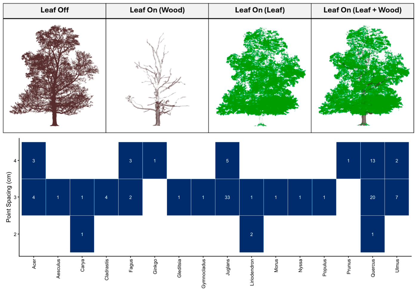
We ran GBSeparation on all our 110 trees and based our workflow on the provided GBSeparation,py script, using Python 3.11. First, we imported each leaf-on TLS point cloud as an XYZ coordinate matrix. We down-sampled each cloud using the downsample_cloud() function from downsampling.py to reduce the computational demands of processing millions of essentially redundant points in a point cloud needed to get the algorithm to converge. We started with a down-sampling resolution of 2 cm. If the model failed to converge, we increased the down-sampling resolution by 1 cm and re-ran the workflow until the algorithm converged and leaf removal succeeded. Some scanned trees were excluded from this study because we were never able to get GBSeparation to converge; these were generally poorly-scanned trees with too much occlusion in the interior of the crown. GBSeparation can get stuck in an infinite loop where no valid neighbor points are found in the graph. An example tree and the resolutions used for final leaf removal for each tree are shown in Figure 1.

After down-sampling, GBSeparation calculated tree height from the vertical range of the point cloud and estimated the root point from the lower 0.2 m of the stem using getRootPt(). GBSeparation appended the estimated root point to the cloud and used it as the graph root. It then constructed a network graph from the down-sampled point cloud using nearest-neighbor relationships, with neighborhood thresholds scaled by tree height. GBSeparation extracted shortest-path distances and paths from the root point through the graph. It identified initial wood points using graph path structure, distance intervals, and angular constraints. GBSeparation then used these initial wood points to classify the final set of wood points across the full graph. After classification, GBSeparation removed the inserted root point and separated the down-sampled point cloud into wood and leaf classes using the final wood mask. Finally, we manually exported the classified wood and leaf point clouds as separate text files for each tree (an example tree is shown in Figure 1). This added a leaf-removed point cloud (e.g., Leaf-On Wood’ in Figure 1) to the leaf-off and leaf-on point clouds for each tree to be run through the TreeQSM algorithm. Note a small portion of the base of the tree was classified as leaves by the algorithm (Figure 1).

We used TreeQSM v2.4.1 to generate QSMs of our study trees, following [25]. For our input parameters, we used TreeQSM’s define_input() function to initialize the QSM parameters. We left all parameters at the default setting, except the following. We set PatchDiam1 to 0.01 m, PatchDiam2Min to 0.005 m, PatchDiam2Max to 0.01 m, BallRad1 and BallRad2 to 0.02 m, and nmin1 and nmin2 to 1 point. These initial parameters ensured we could extract a maximum level of detail equal to the spacing in our point clouds. We visually inspected the results to ensure the QSM represented the tree’s topology well. If there were large topological errors in the QSM, we increased the patch diameters and ball radii until topological errors were minimized. Once we found the optimal input parameters, we generated 10 QSMs for each tree with these input parameters. TreeQSM automatically selected the final, optimal QSM from the 10 QSMs. A final optimal QSM was created for the leaf-on, leaf-off and leaf-removed point clouds for each tree from TreeQSM.

Next, we adjusted each QSM using the run_rTwig() function from rTwig to correct the optimal QSM. The rTwig method forces every branch to end in a realistically-sized twig and models the rest of the branch path behind it to taper realistically. A complete description of the steps in rTwig are presented in [26], but briefly rTwig: (1) determines every path from tree base to each twig (twigs are the terminal cylinders in the branching network of the QSM), so that the total number of paths is equal to the number of twigs in the tree; (2) for each path, a filter is used to remove cylinders of unrealistic size and a monotonic generalized additive model is fit to the remaining cylinders along the path, to determine the correct tapering of the branch path. The intercept of the model is forced to pass through a terminal cylinder (twig) of a realistic size for the species (a twig radius from a measured or published value) and the end of the path. The resultant model then corrects any poorly modeled portions of the QSM. This is repeated for all branch paths in the tree, here with the twig_radius parameter set to the species-specific twig measurements for each tree (data available in [26]). This created three rTwig-corrected QSMs for each tree, leaf-on, leaf-off and leaf-removed. In the end, there were six different final, optimal QSMs for each tree: leaf-on, leaf-off and leaf-removed with and without application of rTwig.

Tree volume and other metrics were computed using the tree_metrics() function to compare different versions of each QSM, including stem diameter at breast height (1.3 m above ground) and the volume of all parts of the tree within different branching orders (this is obtained by summing the volume of all cylinders from that portion of the branching network). The main stem is the 0th order. For all subsequent analyses, we considered the leaf-off point cloud, with the rTwig correction, to be the “reference” value, since [25] demonstrated that this approach produced model trees very similar to measured values from destructively sampled trees of a wide variety of sizes and species.

To analyze the performance of each step in the QSM generation process, we plotted the volumes from each scenario against the reference volume and fitted regression models using a 1:1 relationship as the benchmark for success, e.g., a perfect leaf-removed volume would be the same as the leaf-off refence volume for a tree. The scenarios were (1) TreeQSM leaf-off, without GBSeparation or rTwig; (2) TreeQSM leaf-on, without GBSeparation or rTwig; (3) TreeQSM leaf-on, with GBSeparation, without rTwig; (4) TreeQSM leaf-on, without GBSeparation, with rTwig; and (5) TreeQSM leaf-on, with GBSeparation and rTwig. For each scenario, the slope of the regression lines was compared to a 1:1 line to judge the magnitude of divergence from a perfect representation of the leaf-off reference. E.g., a slope of 2 would indicate an overestimate of 2× and a slope of 0.5 would indicate 0.5× relative to the 1:1 relationship.

2.3. Testing a Field-Calibrated Allometric Model for Predicting Leaf-Off Volume from Leaf-On QSMs

As a final analysis, we examined the possibility of predicting the leaf-off volume from QSMs generated from point clouds of trees scanned in the leaf-on condition. We used a prediction model based on allometric scaling theories (e.g., [38]), which demonstrate that the volume of a tree should scale exponentially with DBH (the stem diameter at breast height (1.3 m above ground) of the tree), but also with recognition that there is a high degree of tree-to-tree variation in such models [39,40]. We hypothesized that including the estimated leaf-on volume of each tree would improve prediction accuracy. This field-calibrated allometric model for predicting leaf-off woody volume was specified as:

$$V_{OFF}={b_0+b_{1}DBH}^{b_2}+{b_{3}V}_{ON}+\mathcal{e}$$

(1)

where V_OFF (m³) is the leaf-off volume of the tree from a QSM corrected with rTwig and DBH (cm) and V_ON (m³) are the stem diameter at breast height and leaf-on volume for the same tree obtained from the leaf-on QSM corrected with rTwig, and b₀, b₁, b₂, and b₃ are parameters estimated by regression analysis; e represents residual error not explained by the model.

We fit the model using generalized least squares regression and used the correlation coefficient and the Root Mean Square Error (RMSE) to measure the overall performance of the model. We also computed the mean bias = Σ(V_OFF predicted − V_OFF measured) and mean relative bias = (mean bias/mean V_OFF measured) to determine if any prediction bias existed and its relative magnitude. All analysis were performed in custom code written in R (version 2025.05.1).

3. Results

3.1. Computational Times for the Different Processing Steps

While processing the point clouds, we found that, on average, it took about 33 min to process a leaf-on tree completely, and about 99% of processing time was to run the GBSeparation LWSA on the point cloud. In general, the processing times for all steps increased with the size of the tree (DBH, cm,

Table 2. Time to process a tree (seconds) during different processing steps.

DBH Class	Leaf Removal	TQSM_ - Leaf Off	TQSM_ - Leaf On	TQSM_ - Remove	rTwig_ - Leaf Off	rTwig_ - Leaf On	rTwig_ - Remove	Total Time
(0, 20]	390.105	1.180	1.037	0.202	0.223	0.011	0.116	392.873
(20, 40]	1547.283	1.245	1.127	0.228	0.222	0.012	0.179	1550.296
(40, 60]	5388.767	2.667	2.658	0.225	0.257	0.013	0.502	5395.089
(60, 80]	8552.581	8.290	10.800	0.295	0.418	0.010	0.944	8573.337
(80, 100]	614.079	16.018	11.888	0.306	0.406	0.010	1.194	643.901
(100, 120]	1168.859	15.406	6.882	0.324	0.357	0.008	1.139	1192.975
(120, 140]	1259.043	21.643	14.171	0.314	0.379	0.007	1.399	1296.957
(140, 160]	872.120	24.560	41.860	0.300	0.738	0.007	2.088	941.672
All trees	1928.916	6.036	5.137	0.248	0.291	0.011	0.553	1941.193

), except for the LWSA, which did not show a distinct pattern with tree size. The LWSA is proportional to the number of points in the point cloud and should be related to tree size. However, if there is any occlusion, greater than the point cloud spacing (such as that created by leaves), it will keep searching for valid neighboring points, which explains why some smaller trees can have taken longer than some larger ones. Overall, the LWSA took a slightly smaller proportion of the total time for larger trees (the lowest was 93%). The other steps took only seconds, with the largest trees taking about 2 min to process.

3.2. The Effects of Leaves and Leaf Removal on QSM Generation and Volume Estimation

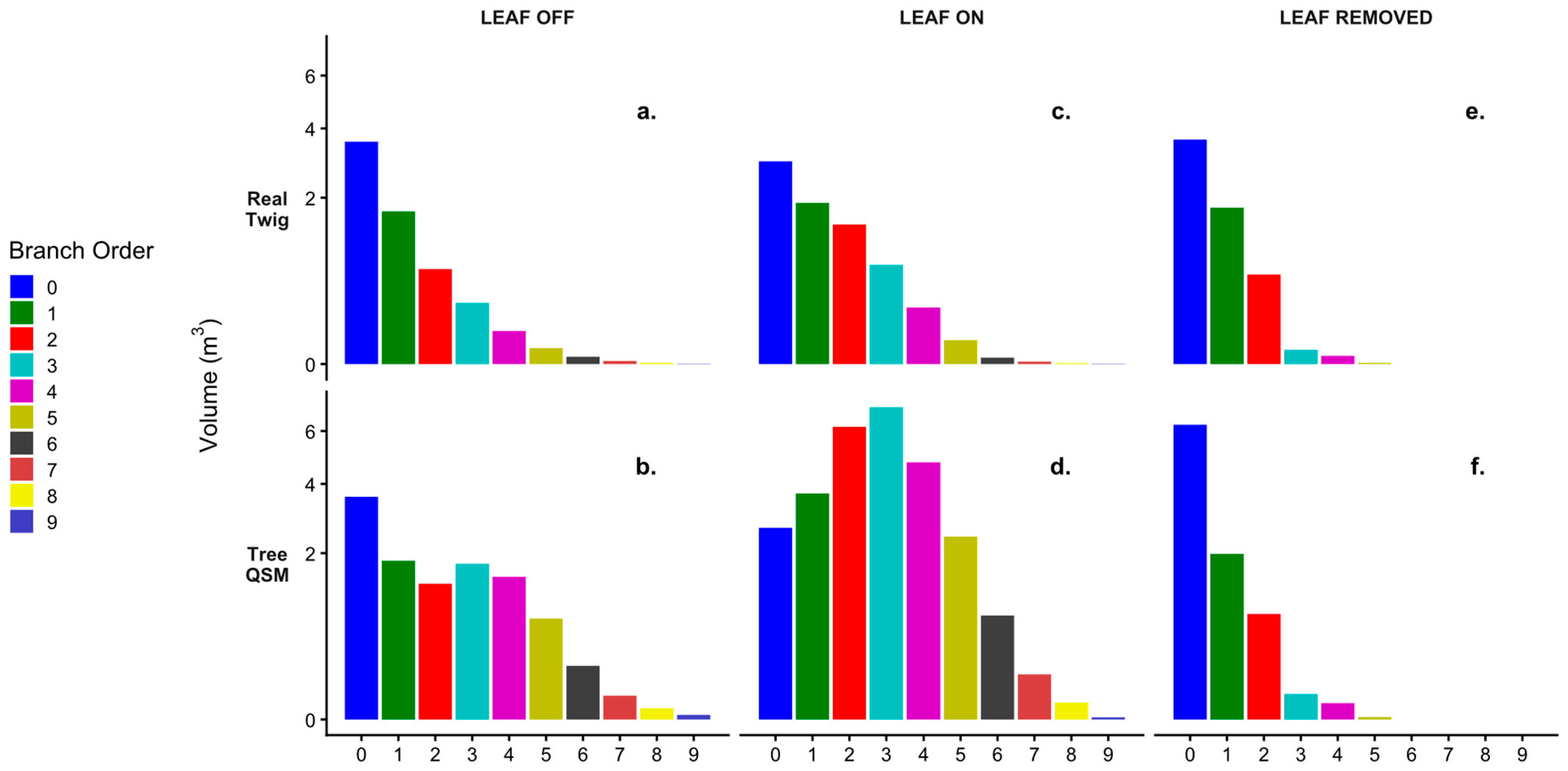
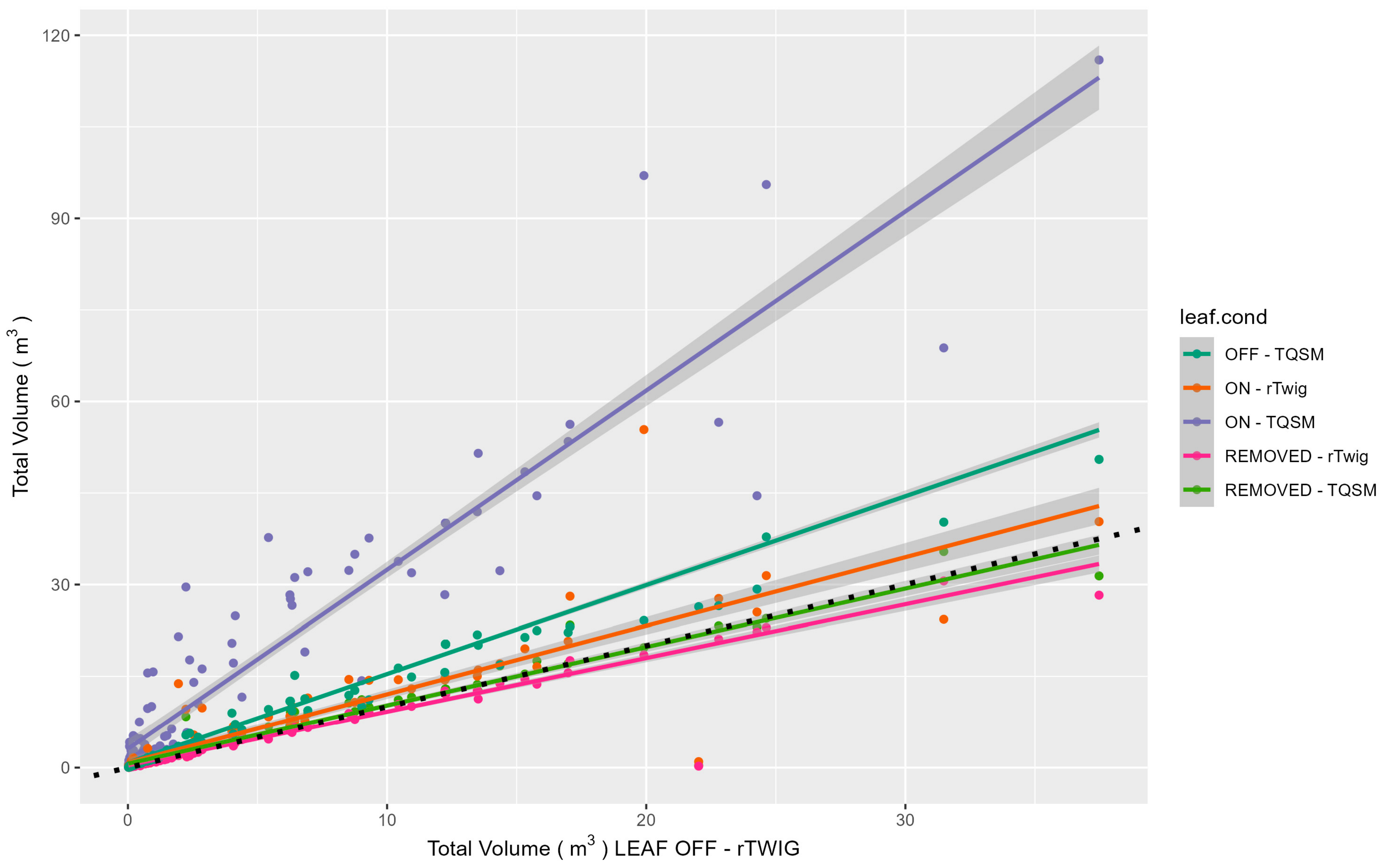
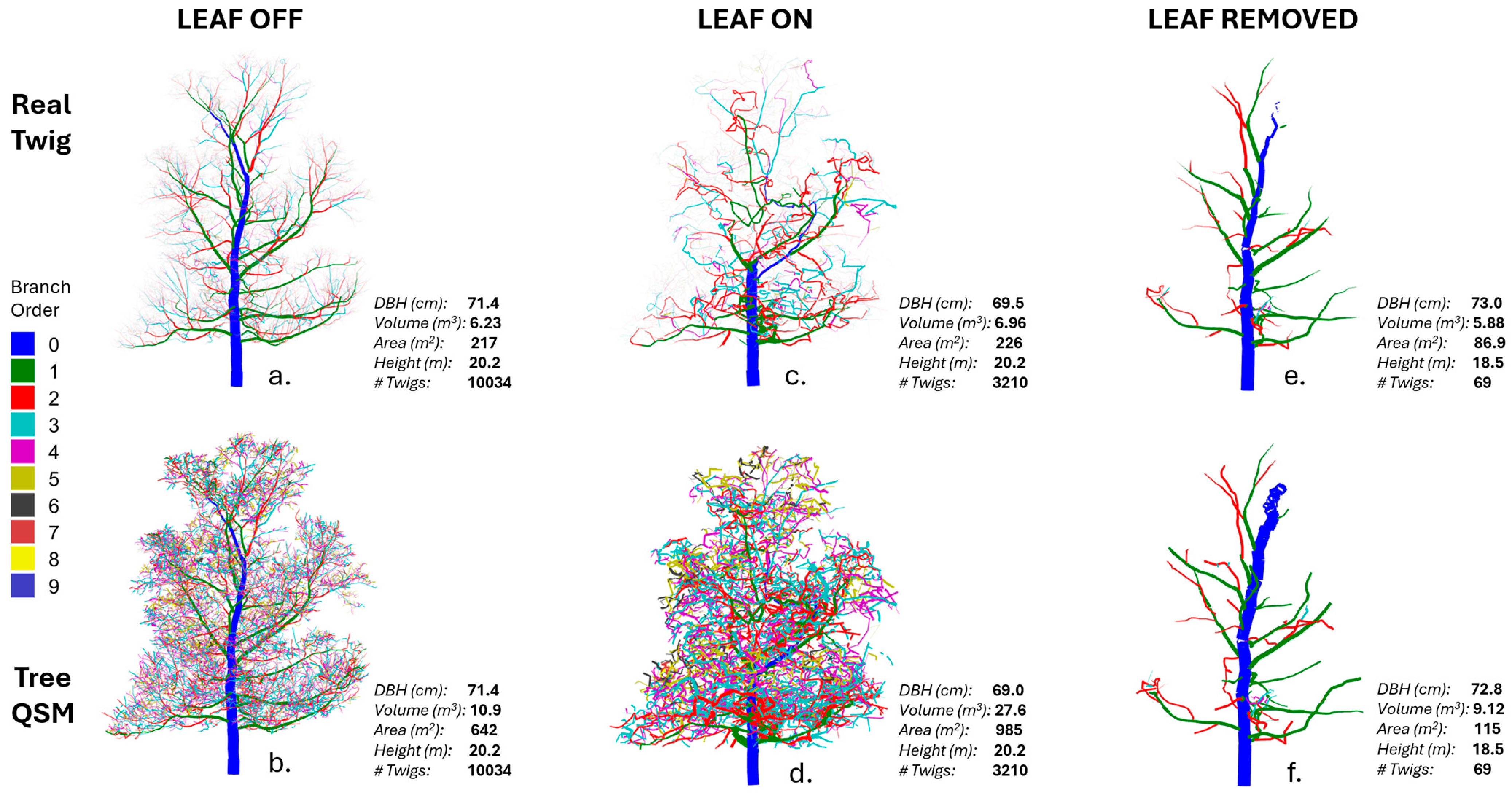
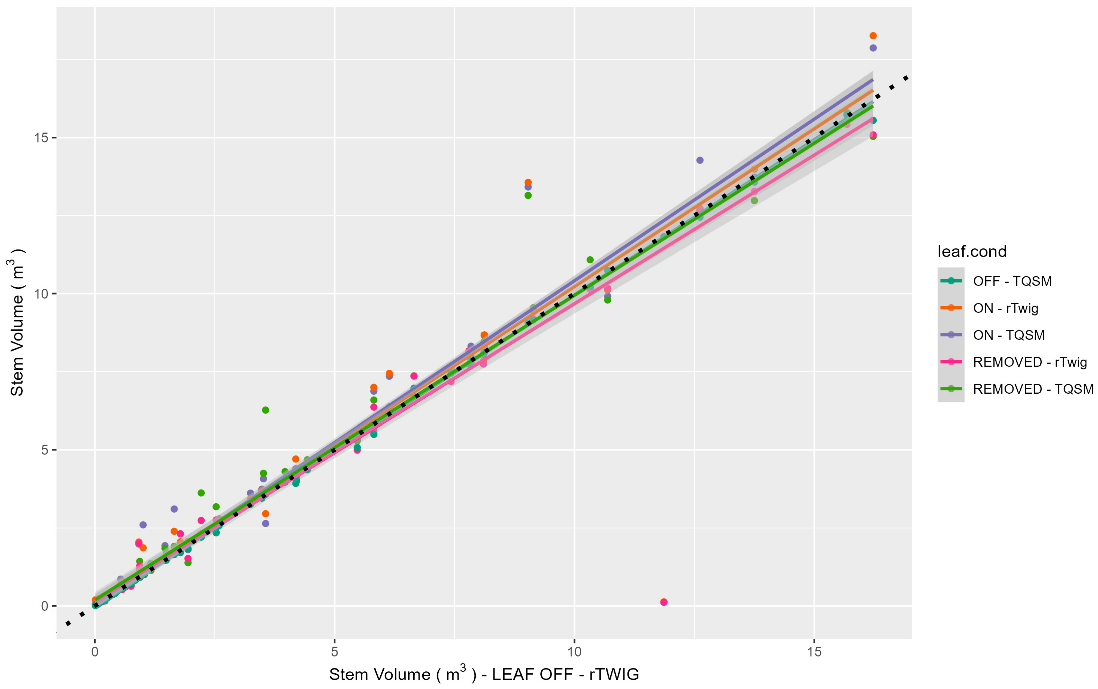
When TreeQSM was applied to trees in the leaf-off condition, trees had about 1.5× more volume on average compared to the reference values (leaf-off rTwig; x axis in Figure 2). The nature of the overestimation can be seen by visualizing an example tree (Figure 3) and looking at the distribution of volume within that tree (Figure 4); volume is overestimated in the higher order branches (i.e., smaller branches and twigs, compare Figure 3a,b and Figure 4a,b).

When TreeQSM was applied to leaf-on point clouds, total volume was about 3× that of the reference values (Figure 2). Overestimation in the leaf-on condition was a combination of inflation of small branches and twig diameters (Figure 3b and Figure 4b), but also the creation of additional branches in the leaf noise by the TreeQSM algorithm (Figure 3d and Figure 4d), which did not exist in the real tree. On average, about one-third of the overestimation error comes from TreeQSM inflating twigs and small branches that were “seen” by the laser (slope of the regression line for ‘OFF-TQSM’ in Figure 2), and the other two-thirds from creating extra branch materials among the leaves and leaf noise that were not branches (slope of the regression line for ‘ON-TQSM’ in Figure 2).

When the rTwig algorithm was applied to reshape the models created by TreeQSM from leaf-on point clouds, the volume was still slightly overestimated by about 1.1× (Figure 2, ‘ON-rTwig’). This additional volume was also from TreeQSM creating non-existing branches from the leaves. In many of the QSMs examined in this condition, TreeQSM created long, winding branches following the leaf surface of the crown, which can be seen more easily in the leaf-on QSM of the example tree with the rTwig correction (Figure 3c) where the additional volume appears in higher order branches (Figure 4c).

Applying GBSeparation to the leaf-on point cloud before processing with TreeQSM resulted in very similar volume, on average, to the leaf-off reference trees (Figure 2). However, examination of QSMs, and volume distribution within trees, demonstrated that the apparently accurate total volume estimation can be the result of counterbalancing errors; i.e., higher order branches are inadvertently removed by GBSeparation, but the remaining parts of the tree accumulated additional volume (Figure 3f and Figure 4f). In the example tree it was most notably the main stem (0th-order branch in Figure 3f and Figure 4f), though this was not always the case. In some cases, the main stem was occluded by leaf noise in the point cloud, leading TreeQSM to try to follow a circuitous path to the top (Figure 3c). Nonetheless, the main stem was the most consistently estimated part of the tree, in general (Figure 5) and most of the total volume error was in the branch volume estimates, which closely follows the pattern shown for total volume in Figure 2.

Applying rTwig to QSMs processed with both GBSeparation and TreeQSM resulted in a slight underestimation bias on average (Figure 2). This happened because GBSeparation classified more higher-order points in the point cloud as leaves, than vice versa, which are then ‘pruned’ out of the point cloud, leaving shortened terminal branches in the QSM, the smallest ends of which rTwig assumes are the size of twigs. This led to over-tapering of the branch ends and volume reduction in the remaining branches (this reduction can be clearly seen in the 4th, 5th and 6th order branches in Figure 3e and Figure 4e).

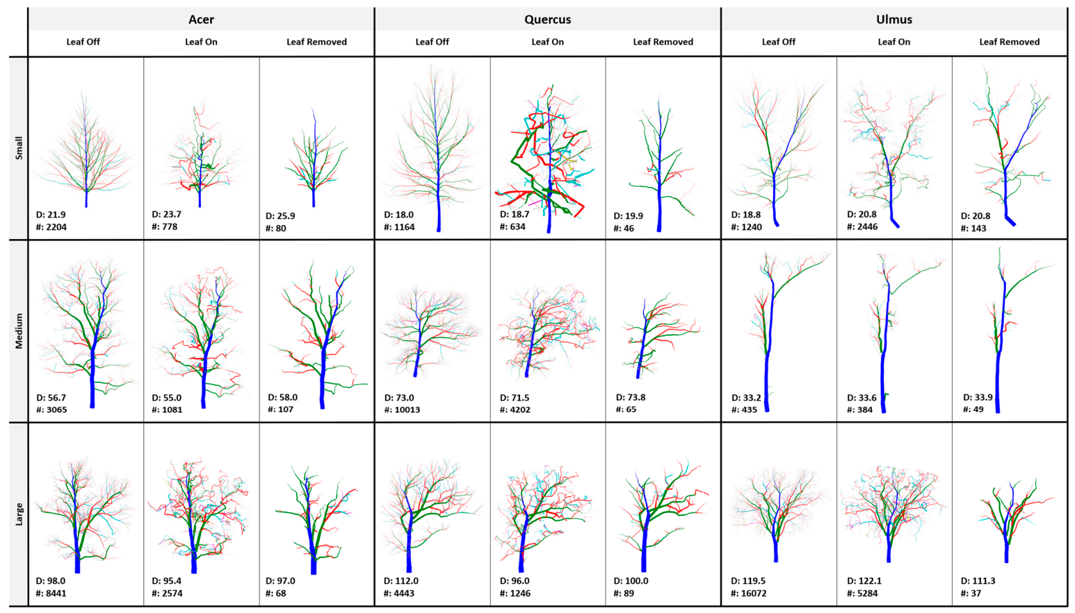
Looking at larger selection of trees of different sizes and species, with the rTwig correction (Figure 6), we can see that leaf-off scans processed with rTwig produced highly realistic QSMs of trees and that application of GBSeparation generally produced reasonably accurate QSMs of the woody portions of the trees, except for omission of small branches and twigs, which were either misclassified as leaves and removed, and/or leaf occlusion left too little data for the QSM to construct fine branches. This left a decrease in the number of twigs in the QSM by two or three orders of magnitude (Figure 6). While many of the leaf-on point clouds also produced QSMs that coarsely resembled the woody skeletons of the trees, they often contained empty spaces in the crown’s interior, where occlusion blocked the scanner from registering hits, but also too much volume on the crowns exterior; this resulted in a greatly reduced number of twigs (about ¼ to ½ of that found with a leaf-off point cloud, and fewer, longer, winding branches with unusual bends and curves (Figure 6)). While rTwig was able to reduce the volume overestimation by tapering the branch ends, it could not overcome the inherent difficulty of constructing the branching topology with occlusion and leaf noise (compare leaf-on trees to others in Figure 6).

3.3. Prediction of Leaf-Off Volume from Leaf-On Point Clouds and DBH Measurement

The field calibrated hybrid allometric model simplified to:

$${\mathit{V}}_{\mathit{O}\mathit{F}\mathit{F}}={{\mathit{b}}_{\mathbf{1}}\mathit{D}\mathit{B}\mathit{H}}^{{\mathit{b}}_{\mathbf{2}}}+{{\mathit{b}}_{\mathbf{3}}\mathit{V}}_{\mathit{O}\mathit{N}}+\mathcal{e}$$

(2)

because the model intercept, b₀ (in Equation (1)) was not statistically different from zero. The parameter estimates and statistical characteristics of Equation (2) are shown in

Table 3. Parameter estimates and statistics for Equation (2).

Parameters	Estimate	Std. Error	t Value	Pr (>|t|)
b1	1.83 × 10−1	3.59 × 10−2	5.103	1.22 × 10−6 ***
b2	1.23 × 10−4	5.16 × 10−5	2.382	0.0187 *
b3	2.41 × 100	8.46 × 10−2	28.527	<2 × 10−16 ***

Significance codes: *** = 0.001; * = 0.05. Residual standard error, e = 1.435.

, below.

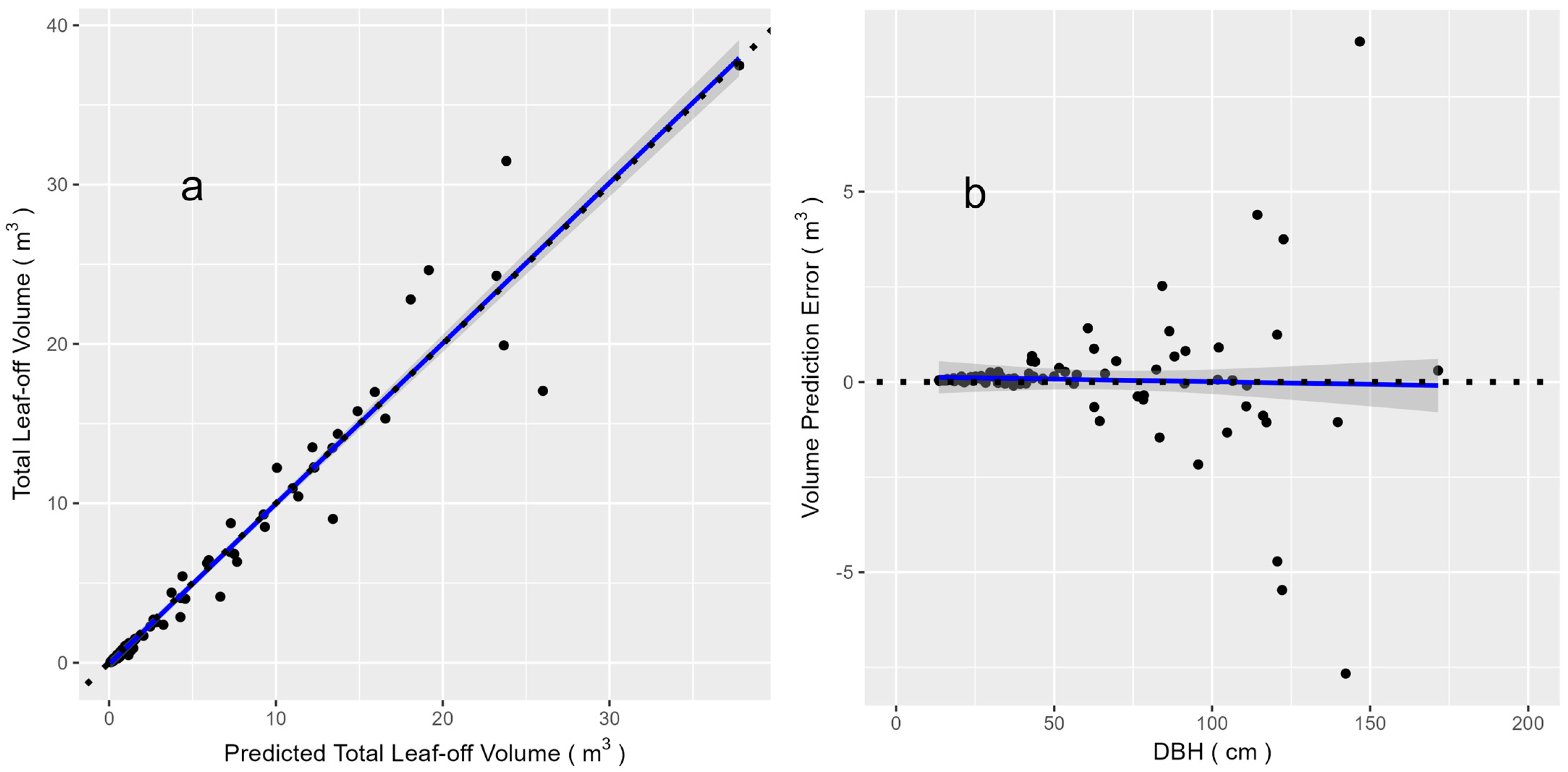
The prediction model performed well over a very large range of volumes (R² = 0.978, RMSE = 1.42) (Figure 7a), with a very low prediction bias (mean bias = 0.051 m³, mean relative bias = 0.78%), although the prediction error increased with tree size (DBH, Figure 7b). We tested a reduced model without the use of DBH and the model still performed well (R² = 0.928, RMSE = 1.425, mean bias = −0.291 m³, mean relative bias = −4.43%). The lack of a statically significant intercept in the prediction models indicated that the leaf-off volume was roughly proportional to the sum of the leaf-on volume estimate and an exponent of the DBH of the tree.

4. Discussion

Our study design allowed us to disassemble different aspects of the process of generating a QSM from tree point clouds scanned in leaf-on and leaf-off conditions, with and without a correction for small branch and twig overestimation, and with and without the application of a high-quality LWSA. This enabled us to determine the influence of leaves and artificial leaf removal on generation of accurate tree models and important tree metrics, here the total tree, stem and higher order branch volumes, of open-grown deciduous trees of a variety of sizes and species, which gave new insights into how specifically leaves affected generation of accurate QSMs of trees.

4.1. Effect of Leaves and Virtual Leaf Removal on QSMs

The most surprising result was that, even though leaves blocked the scanner from registering hits on some branches (Figure 1, top), the confusion of leaves, twigs and small branches around the crown periphery led to overestimation of volume by the QSM algorithm. Our expectation was that leaf-occlusion would lead primarily to underestimation of volume, because parts of the upper stem and branches would be missing and we can see from our analysis that such crown gaps from missing branches do exist (see e.g., the small Quercus in Figure 6). Ref. [25] noted that TreeQSM version 2.4.1 dynamically explores the point cloud to find more, higher order branches, when compared to older versions (2.0–2.3.x) which omit some branches and have a strictly enforced taper, regardless of the underlying point cloud (this result was confirmed to the authors in an unpublished analysis by Pasi Raumonen, the creator of TreeQSM). This advantage of TreeQSM version 2.4.1 in providing a better fit to the input point cloud, i.e., finding more branches and providing a more realistic topology of the tree, came at the expense of attempting to find high-order branches and twigs amongst the leaf noise. We do not consider this a flaw in TreeQSM, per se, which has been shown to produce nearly ‘perfect’ digital twins of real trees for volume estimation from ‘perfect’ point clouds created in a virtual environment [41]. Rather, this points to the ongoing challenge of separating leaves from woody parts of trees and from fitting cylinders amongst any kind of noise and connecting points together to follow the branching architecture of the tree.

Leaf-separation algorithms take on this challenge of “leaf noise” during the point cloud-processing stage. Our results suggest that GBSeparation is generally effective at separating leaves from woody points (see e.g., Figure 1), confirming the validation results of [32,33]. However, this study highlights that GBSeparation can inadvertently remove woody parts, especially high-order branches and twigs, from the point cloud, while successfully removing leaves. Our study quantifies that it can reduce the number of twigs in the tree by two to three orders of magnitude (see Figure 6) and may only give accurate tree total volume estimates through the counterbalancing errors of reducing volume overestimation associated with small branch inflation, by removing smaller branches, but adding additional volume in the remaining parts of the tree (see Figure 4). This might be acceptable if the goal of the laser scanning campaign were simply to estimate volume, biomass or carbon storage, especially for very large trees where twigs and small branches make up a very small portion of the total volume [25]. However, this would, for example, reduce the ability of researchers to use the model tree in simulations of wind dynamics [42,43]. For example, Ref. [44] showed that the sway frequencies of trees with branches removed were significantly higher than those of the same trees with the branches intact.

It is important to acknowledge that we used a phase-shift scanner, which might have generated a greater amount of noise, as compared to the time-of-flight scanner (a RIEGL VZ-400) used by [31], which could have created a bigger challenge for both GBSeparation and TreeQSM. However, a study by [20] showed similar difficulty in reconstructing higher order branches in QSMs generated for leaf-on trees in the tropics when using a RIEGL VZ-400. For GBSeparation, the smaller beam diameter and divergence for the FARO might also have given more detail for measuring smaller branches and twigs [26], but we expect a less noisy point cloud would have made the LWSA more effective and efficient. It would be useful for a future study to have a controlled data set where time-of-flight and phase-shift scanners are tested side by side to determine if a different scanner would have had a major effect on the results. Nonetheless, examination of various tree models produced (Figure 3 and Figure 6) shows that GBSeparation provided a certain level of phase-shift noise reduction to improve reconstruction of larger, lower order branches by TreeQSM.

Our study also revealed a limitation of the rTwig methodology, that it inherits uncertainty and uncorrectable errors from the QSM. The rTwig algorithm assumes that the highest order branch identified by the QSM is the twig and then remodels the taper of the stem and all branches accordingly. If twigs are removed by an LWSA then the remaining small branch stubs are then assumed to be the size of a twig in the tree. Our analysis shows that applying both rTwig and an LWSA can lead to a slight underestimation of branch volume (it had very little effect on the main stem; 0th order in Figure 4a,c,e). Overall, this suggests that the rTwig + GBSeparation combination creates the best balance between a realistic-looking tree model and close to true volume from a leaf-on point cloud; though likely with a slightly conservative estimate of total volume because the highest-order branches are missing (e.g., Figure 4e).

4.2. Predictive Modeling—An Alternative to Leaf–Wood Separation Algorithms

The predictive model worked very well, in general terms, as an alternative pathway to using a LWSA such as GBSeparation. The increasingly larger amounts of prediction error are likely because larger trees are more complex and could be more difficult to scan in the leaf-on condition. We expect the challenge might be even greater in a closed-canopy forest, instead of the open-grown urban conditions we scanned the trees in.

The theoretical part of the predictive model showed an exponential increase in the woody volume of a tree proportional to DBH^2.41. This predictive (allometric) element of our model is not new, as it has long been known that DBH is an easy-to-measure and excellent predictor of many other size-related attributes of trees (e.g., height, biomass), though it does not necessarily need to be specified as a power function [45]. However, to our knowledge, no previous study has suggested combining a DBH-based allometric equation with a LiDAR-based estimate to field-calibrate the allometric model to be more accurate for each individual tree, in this case, estimating leaf-off attributes from leaf-on scans of trees. Looking at the diversity of tree types in Figure 6, we can see that while QSMs are sometimes poorly constructed from leaf-on scans, the leaf-on QSMs still capture the basic shape of the tree registered in the point cloud (Figure 1), which probably gives a unique characterization of that tree, whereas DBH can be a more general metric of size.

There are multiple reasons to employ this type of field-calibrated allometric model (i.e., Equation (2)). First, DBH is the easiest attribute of a tree to accurately measure, manually, or with TLS or MLS [10]. However, the large amount of tree-to-tree variability in DBH-based allometric models suggests the need for local calibration to avoid bias. For example, Ref. [40] estimated that ‘allometric’ uncertainty contributed 30–75% of total uncertainty in tree biomass estimation, suggesting that local calibration is essential. Our field-calibrated approach proposes to use the leaf-on scans for direct calibration of the leaf-off allometric model at the individual tree level. Inventories with TLS should generally have an accurate DBH for each scanned tree [10], but a generic allometric model would likely have a biased estimate of woody volume from the leaf-on scans [40]; a bias that has been shown here to be roughly proportional to the leaf-off volume.

Another benefit of this field-calibrated allometric modeling approach is that evergreen trees, which make up a significant portion of all trees worldwide, cannot be scanned in the leaf-off condition, unless they are scanned dead or defoliated. The latter creates a problem, because such trees represent trees that were or are in poor health. A few studies have been conducted where trees were girdled or stressed to create ‘leaf-drop’ and scanned shortly after [18], but this type of data is limited and requires wounding or killing trees. Our model creates a framework for extending such data sets to predict leaf-off conditions from leaf-on conditions. Even in the case of deciduous tree species, there are limited time windows when the data can be collected, largely during the winter or dry season, depending on the forest ecosystem [46,47]. Our generalized modeling approach, calibrated with local LiDAR data (e.g., Equation (1) or (2)), or a similar approach, could be an important part of the solution set for ameliorating the influence of leaf noise on tree measurements and models generated from laser scanning data.

Another benefit is simply a reduction in computation time. While ground-based and airborne LiDAR data acquisition is becoming increasingly highlighted as an approach to reducing the time cost and efficiency of forest inventory, the time cost and expense of processing massive amounts of remotely-sensed data needs to be given more attention [5,47,48,49]. Given the large investment of time to process tree data created when using a LiDAR-based forest inventory, in this case of a species-diverse urban forest, it is important to consider the computation time to create metrics for each tree or a whole forest [50]. It took about 33 min to process each tree in this study, but less than 1 min if the LWSA was not included. Thus, for the 110 trees in this study, it took about 61 h to process all of them with the LWSA, and <1 h without the LWSA applied. By contrast, it took about 100 h to collect all the field data (about 50 h for the leaf-on and 50 h for the leaf-off scans) and about 600 h to manually separate and check every tree’s point cloud before applying the algorithms to them. So about 8% of the total time needed to obtain the study data was processing the final extracted and checked point clouds for each tree, the majority of which was running the LSWA.

Note, for the processing (Table 2), we used a workstation with an Intel Core i9-13900K CPU, and 64 GB of DDR5 RAM, to process the data. Of course, higher speed computing can be made available and the code for LWSAs such as GBSeparation might be made more efficient. However, remote-sensing based forest inventories are becoming increasingly complex, combining multiple sensors (e.g., [51]), so greater computational speeds will not necessarily keep up with increasing data loads. In any event, the predictive model we generated worked quite well and similar models could be calibrated for leaf-on forest inventories and processed without the additional time cost of a LWSA.

5. Conclusions

Overall, our study brings further evidence that TLS- and other-LiDAR-based approaches offer the promise of capturing the complex architecture of trees in incredible detail and allow for the construction of highly-detailed QSMs for computing volume as well as other tree metrics. But it also highlights that the presence of leaves still constitutes a significant barrier to realizing this potential, despite a growing array of tools to improve the quality of the tree models. Here, our analysis of some of the best available algorithms for constructing QSMs from leaf-on point clouds to generate accurate models and volume estimates suggests that future research is needed to (1) further improve the quality and time-efficiency of LWSAs, (2) develop new QSMs or alternatives to them, and (3) collect more global data sets for testing approaches applied to trees in both the leaf-off and leaf-on condition.

References

1. Tomppo, E.; Olsson, H.; Ståhl, G.; Nilsson, M.; Hagner, O.; Katila, M. Combining national forest inventory field plots and remote sensing data for forest databases. Remote Sens. Environ. 2008, 112, 1982–1999. [Google Scholar] [CrossRef] [Scilit]
2. Kangas, A.; Astrup, R.; Breidenbach, J.; Fridman, J.; Gobakken, T.; Korhonen, K.T.; Maltamo, M.; Nilsson, M.; Nord-Larsen, T.; Næsset, E.; et al. Remote sensing and forest inventories in Nordic countries–roadmap for the future. Scand. J. For. Res. 2018, 33, 397–412. [Google Scholar] [CrossRef] [Scilit]
3. White, J.C.; Coops, N.C.; Wulder, M.A.; Vastaranta, M.; Hilker, T.; Tompalski, P. Remote sensing technologies for enhancing forest inventories: A review. Can. J. Remote Sens. 2016, 42, 619–641. [Google Scholar] [CrossRef] [Scilit]
4. Hamedianfar, A.; Mohamedou, C.; Kangas, A.; Vauhkonen, J. Deep learning for forest inventory and planning: A critical review on the remote sensing approaches so far and prospects for further applications. Forestry 2022, 95, 451–465. [Google Scholar] [CrossRef] [Scilit]
5. Fassnacht, F.E.; White, J.C.; Wulder, M.A.; Næsset, E. Remote sensing in forestry: Current challenges, considerations and directions. For. Int. J. For. Res. 2024, 97, 11–37. [Google Scholar] [CrossRef] [Scilit]
6. Holopainen, M.; Kankare, V.; Vastaranta, M.; Liang, X.; Lin, Y.; Vaaja, M.; Yu, X.; Hyyppä, J.; Hyyppä, H.; Kaartinen, H.; et al. Tree mapping using airborne, terrestrial and mobile laser scanning–A case study in a heterogeneous urban forest. Urban For. Urban Green. 2013, 12, 546–553. [Google Scholar] [CrossRef] [Scilit]
7. Donager, J.J.; Sánchez Meador, A.J.; Blackburn, R.C. Adjudicating perspectives on forest structure: How do airborne, terrestrial, and mobile lidar-derived estimates compare? Remote Sens. 2021, 13, 2297. [Google Scholar] [CrossRef] [Scilit]
8. Arseniou, G.; MacFarlane, D.W.; Seidel, D. Measuring the contribution of leaves to the structural complexity of urban tree crowns with terrestrial laser scanning. Remote Sens. 2012, 13, 2773. [Google Scholar] [CrossRef] [Scilit]
9. Hartley, R.J.; Jayathunga, S.; Morgenroth, J.; Pearse, G.D. Tree branch characterisation from point clouds: A comprehensive review. Curr. For. Rep. 2024, 10, 360–385. [Google Scholar] [CrossRef] [Scilit]
10. Stovall, A.E.; MacFarlane, D.W.; Crawford, D.; Jovanovic, T.; Frank, J.; Brack, C. Comparing mobile and terrestrial laser scanning for measuring and modelling tree stem taper. For. Int. J. For. Res. 2023, 96, 705–717. [Google Scholar] [CrossRef] [Scilit]
11. Arseniou, G.; MacFarlane, D.W.; Seidel, D. Woody surface area measurements with terrestrial laser scanning relate to the anatomical and structural complexity of urban trees. Remote Sens. 2012, 13, 3153. [Google Scholar] [CrossRef] [Scilit]
12. Verbeeck, H.; Bauters, M.; Jackson, T.; Shenkin, A.; Disney, M.; Calders, K. Time for a plant structural economics spectrum. Front. For. Glob. Change 2019, 2, 43. [Google Scholar] [CrossRef] [Scilit]
13. Zeide, B.; Pfeifer, P. A method for estimation of fractal dimension of tree crowns. For. Sci. 1991, 37, 1253–1265. [Google Scholar] [CrossRef] [Scilit]
14. Eloy, C. Leonardo’s rule, self-similarity, and wind-induced stresses in trees. Phys. Rev. Lett. 2011, 107, 258101. [Google Scholar] [CrossRef] [Scilit] [PubMed]
15. Åkerblom, M.; Raumonen, P.; Kaasalainen, M.; Casella, E. Analysis of geometric primitives in quantitative structure models of tree stems. Remote Sens. 2015, 7, 4581–4603. [Google Scholar] [CrossRef] [Scilit]
16. Raumonen, P.; Kaasalainen, M.; Åkerblom, M.; Kaasalainen, S.; Kaartinen, H.; Vastaranta, M.; Holopainen, M.; Disney, M.; Lewis, P. Fast automatic precision tree models from terrestrial laser scanner data. Remote Sens. 2013, 5, 491–520. [Google Scholar] [CrossRef] [Scilit]
17. Åkerblom, M.; Raumonen, P.; Mäkipää, R.; Kaasalainen, M. Automatic tree species recognition with quantitative structure models. Remote Sens. Environ. 2017, 191, 1–12. [Google Scholar] [CrossRef] [Scilit]
18. Stovall, A.E.; Vorster, A.G.; Anderson, R.S.; Evangelista, P.H.; Shugart, H.H. Non-destructive aboveground biomass estimation of coniferous trees using terrestrial LiDAR. Remote Sens. Environ. 2017, 200, 31–42. [Google Scholar] [CrossRef] [Scilit]
19. Bærentzen, A.; Rotenberg, E. Skeletonization via local separators. ACM Trans. Graph. 2021, 40, 1–18. [Google Scholar] [CrossRef] [Scilit]
20. Lau, A.; Bentley, L.P.; Martius, C.; Shenkin, A.; Bartholomeus, H.; Raumonen, P.; Malhi, Y.; Jackson, T.; Herold, M. Quantifying branch architecture of tropical trees using terrestrial LiDAR and 3D modelling. Trees 2018, 32, 1219–1231. [Google Scholar] [CrossRef] [Scilit]
21. Arseniou, G.; MacFarlane, D.W.; Calders, K.; Baker, M. Accuracy differences in aboveground woody biomass estimation with terrestrial laser scanning for trees in urban and rural forests and different leaf conditions. Trees 2023, 37, 761–779. [Google Scholar] [CrossRef] [Scilit]
22. Brede, B.; Calders, K.; Lau, A.; Raumonen, P.; Bartholomeus, H.M.; Herold, M.; Kooistra, L. Non-destructive tree volume estimation through quantitative structure modelling: Comparing UAV laser scanning with terrestrial LIDAR. Remote Sens. Environ. 2019, 233, 111355. [Google Scholar] [CrossRef] [Scilit]
23. Demol, M.; Wilkes, P.; Raumonen, P.; Moorthy, S.K.; Calders, K.; Gielen, B.; Verbeeck, H. Volumetric overestimation of small branches in 3D reconstructions of Fraxinus excelsior. Silva Fenn. 2022, 56, 10550. [Google Scholar] [CrossRef] [Scilit]
24. Morhart, C.; Schindler, Z.; Frey, J.; Sheppard, J.P.; Calders, K.; Disney, M.; Morsdorf, F.; Raumonen, P.; Seifert, T. Limitations of estimating branch volume from terrestrial laser scanning. Eur. J. For. Res. 2024, 143, 687–702. [Google Scholar] [CrossRef] [Scilit]
25. Morales, A.; MacFarlane, D.W. Reducing tree volume overestimation in quantitative structure models using modeled branch topology and direct twig measurements. For. Int. J. For. Res. 2025, 98, 394–409. [Google Scholar] [CrossRef] [Scilit]
26. Morales, A.; MacFarlane, D.W. rTwig: An R Package to Correct Overestimated Small Branches and Twigs in Quantitative Structure Models of Trees. Sci. Remote Sens. 2025, 12, 100284. [Google Scholar] [CrossRef] [Scilit]
27. Shu, Q.; Rötzer, T.; Yazdi, H.; Reischl, A.; Ludwig, F. A comparative study of voxel-based leaf area density estimation from quantitative structure models of trees. Sci. Remote Sens. 2025, 12, 100246. [Google Scholar] [CrossRef] [Scilit]
28. Calders, K.; Schenkels, T.; Bartholomeus, H.; Armston, J.; Verbesselt, J.; Herold, M. Monitoring spring phenology with high temporal resolution terrestrial LiDAR measurements. Agric. For. Meteorol. 2015, 203, 158–168. [Google Scholar] [CrossRef] [Scilit]
29. Van den Broeck, W.A.; Terryn, L.; Chen, S.; Cherlet, W.; Cooper, Z.T.; Calders, K. Pointwise deep learning for leaf-wood segmentation of tropical tree point clouds from terrestrial laser scanning. ISPRS J. Photogramm. Remote Sens. 2025, 227, 366–382. [Google Scholar] [CrossRef] [Scilit]
30. Yan, J.; Wang, J.; Liu, X.; Qi, X.; Feng, Y.; Maeda, E.E.; Hu, T.; Liu, L.; Su, Y. A connectivity-based algorithm for wood–leaf separation from terrestrial laser scanning data. Methods Ecol. Evol. 2025, 16, 2836–2857. [Google Scholar] [CrossRef] [Scilit]
31. Chen, S.; Verbeeck, H.; Terryn, L.; Van den Broeck, W.A.J.; Boni Vicari, M.; Disney, M.; Origo, N.; Wang, D.; Xi, Z.; Hopkinson, C.; et al. The impact of leaf-wood separation algorithms on aboveground biomass estimation from terrestrial laser scanning. Remote Sens. Environ. 2025, 318, 114581. [Google Scholar] [CrossRef] [Scilit]
32. Tian, Z.; Li, S. Graph-based leaf–wood separation method for individual trees using terrestrial LiDAR point clouds. IEEE Trans. Geosci. Remote Sens. 2022, 60, 5705111. [Google Scholar] [CrossRef] [Scilit]
33. Li, Z.; Douglas, E.; Strahler, A.; Schaaf, C.; Yang, X.Y.; Wang, Z.S.; Yao, T.; Zhao, F.; Saenz, E.J.; Paynter, I.; et al. Separating leaves from trunks and branches with dual-wavelength terrestrial lidar scanning. In Proceedings of the 2013 IEEE International Geoscience and Remote Sensing Symposium—IGARSS, Melbourne, VIC, Australia, 21–26 July 2013; IEEE: Piscataway, NJ, USA, 2013; pp. 3383–3386. [Google Scholar]
34. Vicari, M.B.; Disney, M.; Wilkes, P.; Burt, A.; Calders, K.; Woodgate, W. Leaf and wood classification framework for terrestrial LiDAR point clouds. Methods Ecol. Evol. 2019, 10, 680–694. [Google Scholar] [CrossRef] [Scilit]
35. FARO Technologies. FARO Laser Scanner Focus3D X 330; FARO Technologies, Inc.: Lake Mary, FL, USA, 2015. [Google Scholar]
36. FARO Technologies. FAROScene, version 202007; FARO Technologies, Inc.: Lake Mary, FL, USA, 2020.
37. Girardeau-Montaut, D. CloudCompare, Version 2.13.0 (Kharkiv). GPL Software. CloudCompare Project: Grenoble, France, 2024. Available online: https://www.cloudcompare.org (accessed on 15 August 2025).
38. Enquist, B. Universal scaling in tree and vascular plant allometry: Toward a general quantitative theory linking plant form and function from cells to ecosystems. Tree Physiol. 2002, 22, 1045–1064. [Google Scholar] [CrossRef] [Scilit] [PubMed]
39. Pretzsch, H.; Dieler, J. Evidence of variant intra-and interspecific scaling of tree crown structure and relevance for allometric theory. Oecologia 2012, 169, 637–649. [Google Scholar] [CrossRef] [Scilit] [PubMed]
40. Vorster, A.G.; Evangelista, P.H.; Stovall, A.E.; Ex, S. Variability and uncertainty in forest biomass estimates from the tree to landscape scale: The role of allometric equations. Carbon Balance Manag. 2020, 15, 8. [Google Scholar] [CrossRef] [Scilit] [PubMed]
41. Abegg, M.; Bösch, R.; Kükenbrink, D.; Morsdorf, F. Tree volume estimation with terrestrial laser scanning—Testing for bias in a 3D virtual environment. Agric. For. Meteorol. 2023, 331, 109348. [Google Scholar] [CrossRef] [Scilit]
42. James, K.R.; Dahle, G.A.; Grabosky, J.; Kane, B.; Detter, A. Tree biomechanics literature review: Dynamics. Arboric. Urban For. (AUF) 2014, 40, 1–15. [Google Scholar] [CrossRef] [Scilit]
43. Zanotto, F.; Grigolato, S.; Schindler, D.; Marchi, L. Identifying wind-tree dynamics with numerical simulations based on experimental modal analysis. For. Ecol. Manag. 2024, 569, 122188. [Google Scholar] [CrossRef] [Scilit]
44. Moore, J.R.; Maguire, D.A. Natural sway frequencies and damping ratios of trees: Concepts, review and synthesis of previous studies. Trees 2004, 18, 195–203. [Google Scholar] [CrossRef] [Scilit]
45. Picard, N.; Rutishauser, E.; Ploton, P.; Ngomanda, A.; Henry, M. Should tree biomass allometry be restricted to power models? For. Ecol. Manag. 2015, 353, 156–163. [Google Scholar] [CrossRef] [Scilit]
46. Wasser, L.; Day, R.; Chasmer, L.; Taylor, A. Influence of vegetation structure on lidar-derived canopy height and fractional cover in forested riparian buffers during leaf-off and leaf-on conditions. PLoS ONE 2013, 8, e54776. [Google Scholar] [CrossRef] [Scilit] [PubMed]
47. Davison, S.; Donoghue, D.N.; Galiatsatos, N. The effect of leaf-on and leaf-off forest canopy conditions on LiDAR derived estimations of forest structural diversity. Int. J. Appl. Earth Obs. Geoinf. 2020, 92, 102160. [Google Scholar] [CrossRef] [Scilit]
48. Guimarães, N.; Pádua, L.; Marques, P.; Silva, N.; Peres, E.; Sousa, J.J. Forestry remote sensing from unmanned aerial vehicles: A review focusing on the data, processing and potentialities. Remote Sens. 2020, 12, 1046. [Google Scholar] [CrossRef] [Scilit]
49. Liang, X.; Kukko, A.; Balenović, I.; Saarinen, N.; Junttila, S.; Kankare, V.; Holopainen, M.; Mokroš, M.; Surový, P.; Kaartinen, H.; et al. Close-range remote sensing of forests: The state of the art, challenges, and opportunities for systems and data acquisitions. IEEE Geosci. Remote Sens. Mag. 2022, 10, 32–71. [Google Scholar] [CrossRef] [Scilit]
50. Reuter, T.; Seidel, S.; Seidel, D. Comparing Two Novel LiDAR-Based Indices for Quantifying Forest Structural Complexity. Ecol. Evol. 2026, 16, e73605. [Google Scholar] [CrossRef] [Scilit] [PubMed]
51. Köthe, K.; Georgi, R.; Hamutenya, J.; Müller, C.; Nghikembua, M.; Pettenkofer, T.; Trumpa, M.; Seidel, D. A novel two-step framework for bush biomass change-detection and quantification in Namibia using ground-and drone-based LiDAR-a pilot study. Biomass Bioenergy 2026, 212, 109270. [Google Scholar] [CrossRef] [Scilit]
Figure 1. Top: The point cloud of an example tree (‘Acer saccharum #6’) processed with GBSeparation. Bottom: Number of sample trees within each genus down-sampled to 2, 3 or 4 cm of resolution to allow GBSeparation to converge on a solution.
Remotesensing 18 02342 g001
Figure 2. Total volume estimates from QSMs generated by TreeQSM for trees in three conditions, leaf-off, leaf-on and leaf-removed, and two adjusted with rTwig, compared to a reference value for the same trees (OFF- rTwig). Dashed line is the 1:1 reference line.
Remotesensing 18 02342 g002
Figure 3. The six different final QSMs for ‘Acer saccharum #6’ shown to illustrate differences in treatment effects on reconstructed tree architecture (branch orders starting with the main stem as the 0th order are color-coded in the legend) and comparisons of important tree metrics. Subfigures: (a) Leaf-Off/Real Twig; (b) Leaf-Off/Tree QSM; (c) Leaf-On/Real Twig; (d) Leaf-On/Tree QSM; (e) Leaf-Removed/Real Twig; (f) Leaf-Removed/Tree QSM.
Remotesensing 18 02342 g003
Figure 4. Total volume computed for ‘Acer saccharum #6’ from QSMs generated by six different processes distributed by branch order. The sum of the total volume equals the volume shown in the corresponding QSMs in Figure 3 (subfigures represent the same QSMs). Subfigures: (a) Leaf-Off/Real Twig; (b) Leaf-Off/Tree QSM; (c) Leaf-On/Real Twig; (d) Leaf-On/Tree QSM; (e) Leaf-Removed/Real Twig; (f) Leaf-Removed/Tree QSM.
Remotesensing 18 02342 g004
Figure 5. Main stem (0th order) volume estimates from QSMs generated by TreeQSM for trees in three conditions, leaf-off, leaf-on and leaf-removed, and two adjusted with rTwig, compared to a reference value for the same trees (OFF- rTwig). Dashed line is the 1:1 reference line.
Remotesensing 18 02342 g005
Figure 6. Quantitative structure models of trees built with TreeQSM corrected with rTwig, with three different input points clouds: (1) leaf-off, (2) leaf-on and (3) leaf-on processed with GBSeparation. Trees shown were drawn randomly from three genera (Acer, Quercus and Ulmus) within three size classes: small = 0 to 30 cm DBH, medium = 31–90 DBH and large = 90+ DBH. D is the DBH (cm) of each tree shown and # is the number of twigs in its QSM.
Remotesensing 18 02342 g006
Figure 7. (a) Predicted versus reference leaf-off volume from leaf-on volume and (b) volume estimation error (predicted – reference) as a function of tree stem diameter at breast height (DBH). Dashed line is the 0 error line.
Remotesensing 18 02342 g007