


Highlights
What are the main findings?
- Convolutional sequence modeling outperformed recurrent modeling for field-scale surface soil moisture estimation under temporal validation, and combining feature–temporal attention within a temporal convolutional network achieved the best overall performance.
- Field-scale surface soil moisture estimation was context-dependent, relying on the integration of SAR backscatter, optical indicators, and local hydro-meteorological and site-specific variables.
What are the implications of the main findings?
- Sequence-aware multi-source deep learning can support growing-season surface soil moisture monitoring within agricultural station networks.
- A time-aligned multi-source fusion strategy can help convert irregular satellite observations into field-scale soil moisture information for agricultural monitoring.
Abstract
Accurate field-scale surface soil moisture (SSM) measures are important for agricultural water management. Conventional satellite SSM products remain too coarse for within-field applications. Here, we developed sequence-aware deep learning models for growing-season SSM estimation by fusing data from Sentinel-1 C-band SAR, harmonized Landsat-8/Sentinel-2 (HLS), and local ancillary datasets. We assembled a multi-source dataset on Sentinel-1 overpass time for 2016–2024 (May–September), yielding 1469 samples and 65 features per sample, including SAR and optical features, meteorological data, soil texture and bulk density, topography, crop labels, irrigation-likelihood flag, and irregular-time-step encoding. We compared long short-term memory (LSTM) and temporal convolutional neural network (TCN) architectures together with attention-augmented variants, including feature attention (FA), temporal attention (TA), and the combined feature–temporal attention (FTA). Models were trained and tested on seven years of data and were validated based on a temporal generalization using combined data of a wet year (2016) and a dry year (2023). The best model, FTA-TCN, achieved R2 = 0.851, RMSE = 0.024 m3.m−3, and MAE = 0.020 m3.m−3 on the withheld validation years, outperforming the base LSTM (R2 = 0.422; RMSE = 0.053 m3.m−3; MAE = 0.043 m3.m−3) and the base TCN (R2 = 0.746; RMSE = 0.034 m3.m−3; MAE = 0.022 m3.m−3). Shapley additive explanations (SHAP) analysis indicated that antecedent precipitation and short-term rainfall accumulations were dominant forcings, while soil texture, elevation, incidence angle, and vegetation indices modulated SSM variability. Satellite-derived features accounted for ~28.5% of aggregated SHAP importance. Overall, the results show that dual-attention temporal convolution can capture field-scale SSM dynamics across wet and dry seasons when satellite signals are coupled with local soil-meteorological-management context.
1. Introduction
Soil moisture (SM) regulates the land–atmosphere exchanges of water, energy, and carbon. It plays a fundamental role in drought/flood early warning, agricultural management, and weather–climate applications [1,2]. For many hydrologic and agricultural applications, surface soil moisture (SSM), which is the water content in the top ~0–5 cm of soil, is the most relevant and rapidly varying layer because it responds strongly to rainfall inputs and evaporative demand [3,4]. Its spatiotemporal variability is shaped by interacting controls such as soil texture, topography, and meteorological forcing [3]. Since agricultural field management and monitoring decisions are made at field scales (tens-of-meters), field-scale SSM information allows for long-term site-specific decisions. However, prediction remains challenging due to stochastic precipitation and nonlinear infiltration-evaporation dynamics [5].
SSM can be retrieved directly at measurement points using dielectric probes that need site-specific calibration for optimal accuracy. However, they scale poorly to landscapes due to cost and representativeness issues [6]. Passive L-band missions (soil moisture active passive [SMAP])/soil moisture and ocean salinity [SMOS]) provide frequent global SSM (~2–3-day sampling) but at coarse resolution (SMAP ~36 km [9 km enhanced]; SMOS ~25 km), which limits field-scale use [3,7]. This motivates the use of finer-resolution synthetic aperture radar (SAR) (e.g., Sentinel-1 operating at C-band), which is all-weather/day–night and sensitive to near-surface moisture via dielectric effects, although its backscatter is influenced by surface roughness, vegetation structure, and incidence angle [4,7]. In croplands, canopy volume scattering can saturate C-band signals and thus reduce the retrieval accuracy of SSM [8]. Optical sensors (e.g., Sentinel-2) provide vegetation/water-stress proxies for indirect SSM estimation, but are constrained by cloud contamination and vegetation effects [7,8]. Multi-sensor fusion typically improves field-scale SSM estimation, with the best performance reported when combining dual-pol SAR, incidence angle/textural metrics, and optical indices [8,9].
Advances in computing and multi-sensor data availability have driven a rapid adoption of machine learning (ML) and deep learning (DL) for SSM estimation [5]. In particular, DL models that fuse SAR and optical features with ancillary variables better capture nonlinear SSM relationships than traditional formulations [2,7]. For instance, Singh & Gaurav (2023) [2] showed that DL architectures generally outperform traditional ML models across multiple sites. Wang et al. (2024) [5] also found that sequence-aware DL models like recurrent neural networks (RNNs) are well suited to SM time series because they learn temporal dependencies between past and current moisture states. Long short-term memory (LSTM) is an RNN architecture designed to capture long-range dependencies in time series and has been shown to perform well for SM prediction [3,5].
On the other hand, convolutional neural networks (CNNs) learn filters over multi-dimensional inputs and are effective for both 2D imagery and 1D sequences in remote sensing data [9]. A temporal convolutional network (TCN) is a 1D CNN for sequence modeling that uses causal convolutions to prevent look-ahead [10] and dilated residual blocks to capture long-range dependencies with stable, length-preserving outputs [11]. Although TCN applications to SM are still emerging, recent hydrology studies confirm that TCNs can match or outperform RNN baselines with efficient training. For instance, Zhang et al. (2023) [12] and Haider et al. (2023) [13] reported TCNs outperform LSTM for groundwater-level prediction.
The DL models, even sequence-based ones, suffer from limited interpretability [14], so attention mechanisms are often added to learn adaptive weights over input features and/or time lags [15]. Several studies in hydrology found that models with attention outperform those without. For example, Ding et al. (2020) [16] and Li et al. (2022) [15] showed that feature attention (FA), temporal attention (TA), and the combined feature and temporal attention (FTA) improve LSTM performance for flood forecasting and SSM prediction, respectively. Wang et al. (2024) found that FA-LSTM is one of the most effective models for SM prediction [5]. Zhang et al. (2024) [17] and Qin et al. (2024) [18] reported that attention-augmented TCN improves multi-lead runoff forecasting.
The scientific question addressed in this study is whether sequence-aware DL can recover field-scale SSM dynamics from multi-sensor satellite observations and ancillary data when evaluated under temporal transfer. Specifically, we aim to: 1—build a time-aligned multi-source feature set by integrating SAR-optical extracted features with local ancillary variables such as meteorological data, soil properties, topography, and crop and irrigation data, which are all suggested in the literature [7,9,19]; 2—quantify the benefit of convolutional sequence modeling relative to recurrent modeling by comparing TCN versus LSTM under identical inputs and validation design; and 3—test whether FA, TA, and/or FTA improves the performance of standard LSTM/TCN. The main contribution of this study is to identify the most effective structure design for accurate SSM time-series estimation between LSTM, TCN, and attention-augmented LSTM/TCN. Our approach allows training sequence models on multi-year station data and evaluating temporal generalization using withheld climatological contrasting years, complemented by an explainability analysis.
2. Materials and Methods
2.1. Study Area and Period
In 2011, Agriculture and Agri-Food Canada (AAFC) established a real-time in situ soil monitoring for agriculture (RISMA) network in Manitoba [6,20]. The study area of this research is an agricultural region of ~145 km2 encompassing nine RISMA stations, located at approximately 80 km southwest of Winnipeg (Figure 1). The region is generally flat and has a humid continental climate with warm summers (~18 °C) and cold winters (~−13 °C), with ~445 mm average annual precipitation [6,7,20].
Figure 1.
Study area and distribution of nine real-time in situ soil monitoring for agriculture (RISMA) stations within SMAP validation experiment 2016 (SMAPVEX16) soil texture map in Carman region, southwest of Winnipeg, Manitoba (MB), Canada. MB4 site appears as part of the RISMA network but was excluded from the model development and validation based on the quality control results of the in situ surface soil moisture (SSM) measurements.
To capture the interannual variability in SM dynamics, we considered a nine-year time series covering (2016–2024). The analysis was restricted to the growing season (from May to the end of September), when the soil is unfrozen and snow-free. This restriction maintains a physically consistent retrieval because snow cover and soil freeze–thaw transitions hinder the interpretation of satellite signals in relation to SSM [7].
2.2. Dataset and Input Features Set Construction
2.2.1. In Situ SSM Data
At each station in the Manitoba RISMA network, three replicate Stevens Hydra Probes (S1, S2, and S3) were installed at the surface and at 5, 20, 50, and 100 cm depths [6]. These probes were locally calibrated and recorded several variables at 15 min intervals, including SM expressed as volumetric water content (VWC) in m3.m−3, and soil temperature in °C [20]. The published Manitoba RISMA station coordinates in Table 1 represent the station infrastructure located at the edge of each agricultural field, whereas the soil pits containing the probes are located approximately 6–30 m inside the fields [21]. Since the exact soil-pit coordinates were unavailable, their approximate positions were reconstructed using the SMAP validation experiment 2016 (SMAPVEX16) field map and crop information [22]. The station coordinates were shifted into the corresponding agricultural fields according to the station-to-pit offset distance reported by AAFC. A 30 m × 30 m satellite-feature extraction window covering each reconstructed soil-pit location was then considered. The “Center” coordinates reported in Table 1 correspond to the centers of these extraction windows. These reconstructed coordinates should therefore be interpreted as approximate rather than surveyed locations. The station locations in this article refer to the extraction window-center coordinates.
Table 1.
Coordinates * (the latitude [Lat] and longitude [Long]) of RISMA station infrastructure, reconstructed soil-pit locations, and centers of the 30 m × 30 m satellite-feature extraction windows for the nine stations, expressed in WGS 84.
For each station, we performed a quality assessment of the in situ SSM data using the triplicate surface Hydra Probe measurements through Bland–Altman diagnostics [23] and a visual screening of the daily time series. The RISMA daily SSM values used for this quality control are reported at midnight central standard time and represent an aggregated value for the preceding 24 h [7]. At MB1, MB2, MB3, MB5, MB7, MB8, and MB9, the triplicate measurements generally showed small mean pairwise differences and followed similar wetting–drying cycles, although occasional probe-specific anomalies were identified. Two defective periods were removed: MB8 probe 2 during May–September 2017 and MB9 probe 3 during May–September 2019, both of which exhibited step-like artifacts and short spikes. For these periods, the SSM was calculated by averaging the remaining reliable probe measurements. At MB6, probe 2 diverged from the other two probes after March 2016 and was therefore excluded. Therefore, SSM was calculated as the average of probes 1 and 3 measurements. MB4 was excluded from the analysis because its probe measurements did not provide a reliable long-term SSM reference. From early 2019 onward, probes 1 and 2 remained nearly constant and failed to capture seasonal wetting–drying dynamics, while probe 3 showed unrealistic behavior throughout the record. Pairwise Bland–Altman diagnostics further confirmed strong disagreement among the three probes. Although pre-2019 measurements were available, they were not retained because no consistently reliable probe combination could be identified across the full study period. Following this quality control procedure, eight RISMA stations remained in situ references for modeling and validation.
2.2.2. Feature Extraction from Satellite Data
Sentinel-1
Sentinel-1A/B C-band (5.405 GHz) SAR images were collected over the study area and period. The images were Level 1 multi-looked ground range detected (GRD) products acquired in interferometric wide-swath (IWS) mode, with VV and VH polarizations for ascending and descending orbits. The output pixel spacing was ~10 m, whereas the effective spatial resolution was coarser (~5 m in range and 20 m in azimuth). The revisit interval was irregular but was generally ~6 days when both Sentinel-1 A and B were operational and ~12 days after 2022 when only Sentinel-1A acquisitions were available. The incidence angle varied only slightly, from 38.40° to 38.70°, minimizing incidence-angle-related variability and supporting a consistent comparison of retrieved backscatter across acquisitions [24]. Sentinel-1 GRD images were preprocessed in Python 3.8 using the Sentinel application platform for Python (SNAPPY) following a standard workflow [25,26]. Processing included application of precise orbit files, thermal- and border-noise removal, Refined Lee speckle filtering using a 7 × 7 window, radiometric calibration to the backscattering coefficient (σ0), and Range-Doppler terrain correction using the 1-arcsecond Shuttle Radar Topography Mission (SRTM) digital elevation model (DEM), with an output grid spacing of 10 m. The processed scenes were subsequently clipped to the study area [27,28]. From each acquisition, we extracted a set of diverse SAR features, including VV and VH backscatter intensities (), incidence angles (θ), polarization combinations as , , and the dual-polarized radar vegetation index () expressed by (). These predictors help characterize differences between surface and vegetation-related volume scattering [29,30]. For each acquisition and each SAR feature, we extracted the arithmetic mean of a 3 × 3-pixel neighborhood centered on the extraction-window center. This spatial averaging was used to reduce residual speckles and small geolocation uncertainties [31]. All backscatter-derived variables were calculated in linear power units to preserve their physical interpretation.
HLS S30
Harmonized Landsat-8/Sentinel-2 (HLS) S30 version 2 (v2) surface reflectance optical images were acquired for the study area and period to characterize vegetation and land surface conditions. The HLS processing framework reduces spatial and spectral inconsistencies among source observations through atmospheric correction, geometric coregistration, bandpass adjustment, quality assurance masking (F-mask) and resampling to a common 30 m grid [32]. Meanwhile, in a Python pipeline, the HLS spectral bands were multiplied by the scale factor of 0.0001 to convert the stored digital values to surface reflectance, and F-mask filtering was used for clouds/shadows/snow. The valid HLS observations were then resampled from their native 30 m grid to the 10 m Sentinel-1 processing grid using nearest-neighbor interpolation and clipped to the study area [19,32]. The HLS and Sentinel-1 processing grids were harmonized through this resampling. The native spatial detail or information content of the HLS observations did not increase [33]. For each acquisition, the optical bands and features listed in Table 2 were calculated on the common processing grid and averaged using the arithmetic mean of 10 m resampled grid cells within a 3 × 3-pixel neighborhood centered on the extraction-window center. Therefore, this neighborhood covered approximately 30 m × 30 m in the common processing grid.
Table 2.
Detailed information on HLS S30 v2 extracted feature set.
Finally, to align the optical features with Sentinel-1 acquisition dates, each HLS feature was interpolated using locally estimated scatterplot smoothing (LOESS) interpolation [34]. LOESS was fitted independently for each optical feature, station, and growing season using only HLS observations from May to September of a given year. The LOESS implementation used a local linear fit with a smoothing fraction of 0.35. The interpolation accuracy was assessed using leave-one-date-out reconstruction of valid interior clear-sky HLS observations. We summarized using the mean absolute error (MAE) in the corresponding feature units. Across the reflectance bands, MAE ranged from 0.022 to 0.033, with the lowest error observed for Red Edge 2 and the highest for Red. For the derived vegetation and water indices, MAE values ranged from 0.029 to 0.042, with the lowest error observed for NDMI and the highest for EVI. CWC exhibited the highest MAE among all evaluated HLS-derived features, at 0.045.
2.2.3. Feature Extraction from Ancillary Datasets
Geographical Data
To explicitly account for the spatial information regarding the monitoring locations and to help the model adapt to site-specific soil–vegetation–climate regimes [1], the input dataset contained each station’s coordinates (Table 1).
Topographical Data
Topographic predictors were derived from the SRTM 1-arcsecond DEM. Elevation, slope, and aspect were extracted at each RISMA station, indicating a low-relief landscape with elevations of 248 m–264 m and gentle slopes of ~1.10–2.46°. Aspect values span multiple directions (approximately 63.4–333.4°, with common orientations near 90°, 180°, and 270°). To improve model interpretability, aspect was decomposed into two continuous components, x and y, using trigonometric transforms [27] and was added to the input feature set in both forms.
Crop Information
For each RISMA station, crop type data was compiled from the annual crop inventory (ACI), a 30 m resolution database, which maps crop types across Canadian agricultural regions [35]. The crop type in the eight fields includes soybeans, spring wheat, corn, beans, oats, and canola/rapeseed during the study period. The distribution per year over the study area reveals a significant interannual variability across stations. The month of year (MOY) acts as a practical proxy for the phenology stage during the growing season [7]. To preserve seasonality and better reflect phenological progression, the MOY was mapped to the unit circle using sine–cosine encoding [27] and was added into the input feature set. These variables were assigned according to the field and acquisition date of each Sentinel-1 overpass. These parameters provide a general phenological context for crops with similar structural characteristics, which help models distinguish vegetation-driven signal changes from SM-driven variability [1].
Soil Parameters
The input dataset includes surface soil texture (sand, silt, and clay fractions), bulk density, and soil-surface temperature derived from the RISMA network. Soil temperature was represented by the 15 min measurement closest to each Sentinel-1 overpass, together with the daily mean, maximum, and minimum soil temperature values. Across the RISMA stations, surface texture spans a strong gradient, from sandy loam soil in the western part of the study area, characterized by high sand and low clay fractions, to clay-dominated soils toward the east, with intermediate loam and clay–loam textures between them. Sand content ranges from ~3.6% to 81.3%, and clay content ranges from ~11.1% to 71.7%, consistent with the west-to-east texture transition in Figure 1. Surface bulk density ranges from 1.21 g/cm3 to 1.53 g/cm3 across the network [20].
Meteorological Data
At each RISMA location, a weather station records meteorological variables at 15 min intervals [20,21]. The input feature set included two temporal representations. First, it contained daily meteorological variables corresponding to the acquisition date of each Sentinel-1 overpass, including mean, maximum, and minimum air temperature, mean relative humidity, mean wind direction, and mean, maximum, and minimum wind speed. Second, it included overpass-matched meteorological variables derived from the 15 min station records closest in time to the Sentinel-1 acquisition, including air temperature, relative humidity, wind direction, wind speed, and the precipitation-occurrence flag. Short-term precipitation accumulations were computed over the 1 h, 3 h, and 6 h periods immediately preceding each Sentinel-1 overpass. Longer antecedent precipitation variables were calculated for the 3-day and 6-day periods preceding the overpass and for the time interval since the previous Sentinel-1 acquisition. Moreover, daily all sky surface shortwave downward irradiance (SDI) and all sky surface photosynthetically active radiation (PAR) were extracted from the NASA prediction of worldwide energy resources (POWER) database for the overpass date.
Irrigation Data
Field-level irrigation records were unavailable for RISMA stations; we thus represented the irrigation information using an approximate crop- and month-specific irrigation-likelihood flag. Approximate irrigation periods for 2016–2024 (Table 3) were inferred from the annual reports of the Manitoba Diversification Centers (MDCs), with monthly precipitation records from Environment and Climate Change Canada (ECCC), and provincial drought summaries [36,37]. These sources helped identify crop-year-specific months when irrigation was likely required. For each Sentinel-1 overpass date, the binary irrigation flag was assigned a value of 1 when the crop type, year, and month of acquisition matched one of the periods listed in Table 3; otherwise, it was assigned 0. This flag represents a coarse proxy rather than a verified record of actual irrigation timing or amount at a RISMA station.
Table 3.
Approximate crop- and year-specific irrigation-likelihood periods used to assign the irrigation flags for RISMA samples during 2016–2024.
Time Space Encoding
We retained only the dates corresponding to Sentinel-1 overpasses during the study period. Because Sentinel-1 revisit intervals are irregular, we included (days since the previous acquisition) as an input. The models can thus account for unequal time lags rather than assuming uniform sampling [38].
2.3. Methodology
Figure 2 presents the overall methodological framework of this study. To ensure temporal synchronization, we had one comprehensive input feature set containing all 65 input features (Section 2.2 and Appendix A) for DL models.
Figure 2.
The overall methodological framework of the study.
2.3.1. Data Split Protocol and Statistical Analysis on In Situ SSM
The target variable () in each DL model was defined as the quality-controlled SSM measurement (Section 2.2.1) derived from the 15 min RISMA surface-probe record closest in time to each Sentinel-1 overpass. Over the full observation period from 2016 to 2024 (May–September), the merged and refined dataset contained 1469 samples with complete records for all 65 input features across the eight retained RISMA stations. To ensure fair comparison across the DL architectures [39], the model was developed using seven years of data from 2017 to 2024 (excluding 2023), totaling 1151 samples. Model generalization was then assessed using an external temporal-validation strategy based on two climatologically contrasting years, rather than by testing spatial transferability to unseen stations.
As shown in Table 4, 2016 had the highest network-mean May–September total precipitation (393 mm) and the highest mean target SSM (0.301 m3.m−3), ranking first for both precipitation and target SSM. In contrast, 2023 had the lowest network-mean May–September total precipitation (141.4 mm) and one of the lowest mean target-SSM values (0.222 m3.m−3). Therefore, the temporal-validation set ( = 318) represents the wettest year (2016) and driest/near-driest year (2023) available in the record.
Table 4.
Growing-season hydroclimatic and target-surface soil moisture (SSM) summary used to justify the temporal-validation years.
For the sequence-based models, each input sample was constructed as a lookback window of consecutive Sentinel-1 overpass records ending at the target overpass date. Each lookback window was labeled according to the year of its target Sentinel-1 overpass. Lookback windows with target years 2016 and 2023 were withheld entirely from model development and used only for external temporal validation. The remaining development sequences were randomly divided into an 80% training subset ( = 920) and a 20% internal test subset ( = 231), which was used for model selection and hyperparameter tuning. In addition to the year-wise hydroclimatic comparison, the target-SSM distributions of the training and validation sets were summarized using the mean (M), standard deviation (SD), and coefficient of variation (CoV) (Figure 3) [19,39]. Figure 3 shows that the external validation set falls within a similar overall SSM range as the training data, meaning the withheld validation years were within the target-variable range represented during model development.
Figure 3.
Violin box plots of targets in situ SSM distributions for the full dataset, and the training and the external temporal-validation sets. The validation set covers a similar SSM value range to that of the training data, so the validation is within the target-variable range of the training data.
A two-sample Kolmogorov–Smirnov (K–S) test [40] was also applied to compare the empirical cumulative distribution functions (ECDFs) of the training and external-validation sets. The K–S test measures the maximum vertical separation between two empirical distributions using the K-S statistic :
where and are the ECDFs of the training and validation target-SSM values, respectively, and denotes the maximum absolute difference over all observed SSM values. The associated -value tests the null hypothesis that both samples originate from the same distribution. The K–S test indicated a statistically detectable distributional difference between the two sets, with D = 0.362 and p = 0.0011, showing that the maximum vertical separation between their ECDFs was 36.2 percentage points. Therefore, the contrasting wet and dry validation years introduce a measurable distributional shift in target SSM compared to the training set. Because ECDF-based two-sample tests assess distribution-level differences rather than only mean differences [40,41], Cohen’s d was also calculated to quantify the standardized mean difference between the two sets (Equations (2) and (3)) [42].
where is the pooled standard deviation and , , and represent the mean, standard deviation, and sample size of each set, respectively. The magnitude of Cohen’s was small (|| = 0.164), indicating that the mean target-SSM difference between the two sets was limited. These results have two implications for interpreting validation performance. First, the external-validation set represents a more challenging temporal-transfer test than a random split, because the models were evaluated over years with different hydroclimatic conditions than those in the training set. Second, strong predictive performance of a model under this measurable distributional shift demonstrates its temporal robustness and generalization capacity within the observed RISMA SSM range under non-identical training–validation distribution conditions.
2.3.2. Feature Scaling
After defining the data split, we standardized continuous input variables using z-score scaling (Equation (4)) to support stable model training, where Sc represents the scaled value, Ini is the original value, and and are the mean and standard deviation calculated from the training set for the corresponding variable [2]. To avoid information leakage, the scaling parameters were calculated for each continuous variable using the training set only and then applied unchanged to transform the internal-test and external-validation sets. The target SSM was standardized using the same training-only principle. The model-predicted SSM was then inversely transformed using and to recover SSM in VWC units (m3.m−3).
2.3.3. Sequence-Aware DL Models
In this study, sequence-to-one DL models, including LSTM, TCN, and their attention-based variants, estimate SSM () at a target Sentinel-1 overpass time index t. The model input is a multivariate historical lookback window , where m represents the lookback window length (the number of Sentinel-1 overpass time steps included in the input sequence). Each row represents a vector of 65 predictors assembled at overpass index k (where ). These predictors include SAR features, HLS features interpolated to the Sentinel-1 overpass date, ancillary variables, and the acquisition time-gap variable (Appendix A). The relative sequence lag of each input step can be expressed as (ℓ = t − k), whereas () represents the elapsed time in days since the previous Sentinel-1 acquisition. By sliding this lookback window through the station-level time series, the complete predicted SSM time series, denoted as , is generated for each station.
LSTM: Figure 4a shows one LSTM cell applied sequentially over the input lookback window. At each overpass index , the cell updates its hidden state and cell state from the current step input and previous states (, ). Figure 4b shows the sequence-to-one setup. After processing the historical steps, the final hidden state at the target overpass time is passed to a dense layer to estimate . The gate operations at each overpass step k follow:
where W and b are learned weights and biases for each gate, σ is the sigmoid activation function, and denotes element-wise multiplication [16,43]. In our context, these gates allow the model to retain or down-weight parts of the historical sequence that are most informative for predicting SSM at the current overpass time t.
Figure 4.
Long Short-Term Memory (LSTM) architecture used for SSM prediction. (a) LSTM cell updating hidden and cell states from the 65-feature input at each overpass step k. (b) Sequence-to-one setup: an input lookback window is encoded, and the final hidden state at the target overpass t is mapped by a dense layer to predict SSM value ().
TCN: The TCN replaces the recurrence with a stack of 1-D dilated causal convolutions applied along the sequential Sentinel-1 overpass axis. Causal means the encoded representation at overpass index is computed only from the current and earlier time steps within the input lookback window. Consequently, the estimated SSM at the target time t () does not use future information, preventing look-ahead bias. The core operator is the dilated convolution (Equation (11)), which computes an output as a weighted sum of past sequence steps sampled every sequence steps. For one temporal feature map (one channel) and filter weights , the output at time-lag index k is:
where is the kernel size (number of kernel elements), is the dilation factor, represents the learned filter weights indexed by , and denotes the value from an earlier step within the lookback window. When , the convolution processes consecutive overpasses; when , it skips intermediate steps to capture longer historical memory without increasing S. Stacking residual blocks with increasing dilation (e.g., ) expands the receptive field to represent both rapid wetting responses and multi-overpass dry-down persistence. Training stability is ensured through residual learning (Equation (12)), where is the block input feature map, is the learned transformation produced by the dilated convolutions and nonlinearities inside the residual block, is the activation function, and is the block output:
This structure helps gradients propagate through deep stacks and lets each block learn a correction to its input rather than relearning the full mapping [18,44]. In our implementation (Figure 5), applying these residual blocks to the multivariate input lookback window produces an encoded sequence . The final encoded vector at the target time step is then passed to a dense regression layer to generate .
Figure 5.
Temporal Convolutional Neural Network (TCN) architecture used for SSM prediction. An input lookback window is encoded by stacked dilated causal residual blocks along the Sentinel-1 overpass sequence, and the final encoded vector is mapped by a dense layer to predict SSM () at the target overpass.
Attention Mechanisms: In this study, we investigated soft attention as a lightweight mechanism that allows the network to adaptively emphasize the most informative features and/or time steps for each overpass. It provides an internal model diagnostic indicating the elements on which the model relied to generate . Rather than selecting a fixed feature subset a priori, attention learns normalized weights (via the function) that reweight inputs or encoded sequences during training. We evaluated three configurations (FA, TA, and FTA) on top of each backbone (LSTM/TCN). FA assigns feature weights (α) across the 65 predictors within each overpass step k. At any given step, the input vector is . A small gating layer produces a raw feature score vector , which is converted into normalized attention weights for each feature channel j (Equations (13) and (14)). The reweighted input vector becomes (Equation (15)). The fully adjusted sequence is passed to the backbone network to produce the representations used to predict .
TA assigns time-step weights (β) to each overpass step k within the lookback window. After the processing by the backbone, we obtain an encoded sequence , where each is the encoded vector of the backbone at overpass step k. TA computes a scalar importance score for each step and normalizes these scores across the lookback window (Equations (16) and (17)). A context vector is then formed as a weighted sum (Equation (18)) and regression head (Equation (19)) produces the final SSM estimate [5,16,18]. Here, represents the relative contribution of overpass step , or equivalently relative lag , to the SSM prediction at the target overpass .
FTA (Figure 6) applies FA first to reweight features within each time-lag step, passes this adjusted sequence to the backbone to generate the encoded sequence , and finally applies TA to aggregate the encoded vectors across the m time steps before sending the representation to the dense regression head. Concretely, maps to via ; maps to via LSTM/TCN backbone; maps to via ; and is mapped to the final prediction . This architecture allows the model to simultaneously optimize which specific features and past overpasses are most relevant to each SSM estimate.
Figure 6.
Feature and temporal attention used with LSTM/TCN for sequence-to-one SSM prediction at target overpass t. (a) Feature attention (FA) reweights each 65-variable input vector using channel weights (), the backbone encodes the lookback window into . (b) Temporal attention (TA) aggregates encoded overpass steps using weights () to form for the final regression output .
2.3.4. Model Architecture and Hyperparameter Tuning
All models were trained for sequence-to-one regression using mean-square error (MSE) as the loss function, Adam as the optimizer, rectified linear unit (ReLU) activations in the dense layers, and a linear output layer. To ensure reproducibility and a fair model-to-model comparison, all experiments used the same fixed random seed (27). The sequence length (m) was treated as a tunable hyperparameter, so the number of usable training and validation sequences varied slightly across models due to sequence constructions.
Hyperparameters were tuned with Optuna, a Bayesian optimization framework, by minimizing MSE on the internal test set. We selected Optuna because it efficiently optimizes mixed and conditional hyperparameters across architectures [45]. During the hyperparameter tuning phase, the internal-test data were transformed using the scaler fitted on the training set (Section 2.3.2). For a fair comparison, all models belonging to the same backbone used identical Optuna search ranges for their architectural settings. For the TCN-family models, the common search space included the number of residual blocks (3–8), kernel size (3 or 5), dropout rate (0.1–0.5), and convolution filters per block (32, 64, or 128). For the LSTM-family models, the common search space included the number of stacked LSTM layers (1–3), hidden units per layer (32, 64, or 128), and output dropout rate (0.1–0.5). All models also shared the same training hyperparameter search ranges. Table 5 presents the best-performing configurations obtained from this protocol.
Table 5.
Best-performing architecture configurations and training hyperparameters obtained from Optuna optimization for each evaluated model.
2.4. Performance Assessment and Interpretation of DL Models
The model performance was evaluated for the growing-season SSM estimation using the coefficient of determination (R2), the root mean-square error (RMSE), and the MAE (Equations (20)–(22)). In these equations, is the observed in situ SSM for sample , is the mean observed SSM, is the predicted SSM for sample , and is the number of evaluation samples [46]. The metrics were computed for each modeling scenario (LSTM, TCN, FA/TA/FTA-LSTM/TCN). Prediction bias was also calculated (), where positive values indicate overestimation and negative values indicate underestimation. The residual error for a single data point was calculated by .
To quantify the statistical uncertainty of the performance metrics, 95% bootstrap confidence intervals (CIs) were computed for R2, RMSE, and MAE using a paired nonparametric bootstrap procedure. For each model, the paired observed–predicted validation samples (, ) were resampled with replacement over 1000 bootstrap iterations. In each iteration, R2, RMSE, and MAE were recalculated from the resampled validation pairs, producing an empirical bootstrap distribution for each metric. The 95% CI was then defined using the 2.5th and 97.5th percentiles of the corresponding bootstrap distribution. Because the optimized lookback-window length differed among architectures, the bootstrap procedure was applied separately to the validation samples available for each model [47,48].
To complement these evaluation metrics, we used Shapley additive explanations (SHAP), specifically SHAP DeepExplainer (DeepSHAP), as the primary attribution method. We selected DeepSHAP because this variant is more computationally tractable than perturbation-based SHAP approaches for deep sequence models [49,50]. For each architecture, we calculated SHAP values on the external temporal-validation set. To quantify the overall contribution of each feature, mean-absolute SHAP values were computed after aggregating feature attributions across the overpasses within the input lookback window.
3. Results
3.1. Performance Assessment of DL Models
3.1.1. Evaluation Metrics
The predictive performance of the DL models on the validation set is summarized in Figure 7 and Table 6. Table 6 reports point-estimates and 95% bootstrap CIs of performance metrics, providing an uncertainty range around the performance metrics. Overall, the bootstrap results support the point-estimate ranking shown in Figure 7.
Figure 7.
Comparative performance of DL models for validation years (2016 and 2023) using root mean-square error (RMSE) (m3.m−3), mean-absolute error (MAE) (m3.m−3), and coefficient of determination (R2) values.
Table 6.
Performance metrics and 95% bootstrap confidence intervals (CIs) for each DL model on the external temporal-validation set.
The base LSTM showed the weakest temporal-transfer performance, while the base TCN achieved better results. Attention integration produced mixed outcomes depending on the base architecture and whether FA and/or TA were combined. For LSTM hybrids, attention substantially improved temporal and feature generalization relative to the base LSTM, with FTA-LSTM showing the strongest performance within the LSTM family. For TCN hybrids, adding only FA or only TA did not outperform the base TCN in this dataset. In contrast, FTA-TCN yielded the best overall performance, with the lowest RMSE (0.024 m3.m−3) and MAE (0.020 m3.m−3), the best point-estimated (0.851), and narrow bootstrap intervals. Relative to the base TCN, this corresponds to an RMSE reduction of ~29%, and relative to the base LSTM, an RMSE reduction of ~55%. The RMSE CI of FTA-TCN was lower than that of the base TCN, supporting the added value of the combined feature–temporal attention mechanism for reducing prediction error. Although FTA-TCN had the lowest overall error, its R2 CI overlapped with that of FTA-LSTM, and its MAE CI overlapped with some TCN-family models. Figure 8 presents scatter plots comparing the predicted and observed SSM on the validation set.
Figure 8.
Predicted versus observed SSM on the external temporal-validation set for each DL model, with point color indicating sample-density concentration. Each panel reports the number of usable validation sequences (N) and the corresponding evaluation metrics (R2, RMSE, MAE). Since the sequence length (m) was tuned separately for each architecture, the number of usable validation sequences differs slightly from one model to another.
The scatter plots show distinct variations in model calibration and precision across different configurations. The base LSTM (Figure 8a) exhibits the highest dispersion, indicated by the broad spread away from the 1:1 dashed line (R2 = 0.422 and RMSE = 0.053 m3.m−3), with a notable tendency to underestimate high SSM values and overestimate dry states. In contrast, the base TCN (Figure 8b) demonstrates a significantly improved alignment (R2 = 0.746 and RMSE = 0.034 m3.m−3), suggesting that in this study, the dilated convolutional structure is better suited for capturing the multi-scale dependencies of SSM than the recurrent approach.
3.1.2. Computational Efficiency Assessment of DL Models
Computational-efficiency results are summarized in Figure 9 and Table 7. Figure 9 shows the training time, the trainable parameter count, and the prediction bias. Training time ranged from ~0.5 to 3.7 min across models, reflecting the compact size of the dataset and early stopping termination under optimized training.
Figure 9.
Accuracy–efficiency comparison of the evaluated DL architectures. Bubble plots show training time versus RMSE (m3.m−3) (a), training time versus R2 (b), and RMSE versus the logarithm of the number of trainable parameters (c). Point colors denote model type, and bubble radius is proportional to the absolute mean prediction bias.
Table 7.
Per-sample inference time measured on consistent hardware for each DL model.
Table 7 reports the per-sample inference time for each DL model. All models were evaluated on the same hardware. Inference time was calculated as the average batched CPU forward-pass time per validation sample, excluding non-model processing steps. Inference time ranged from 0.05 ms/sample for the base LSTM to 0.27 ms/sample for FTA-TCN. Among the non-attention baselines, the LSTM had the lowest inference time and the shortest training time but produced the weakest predictive performance. The TCN required only a bit more inference time and provided a better accuracy–efficiency balance. Adding a single attention improved the LSTM backbone but increased inference cost. In contrast, adding a single attention to the TCN backbone increased inference time but did not improve performance relative to the base TCN. Adding both features and temporal attention had different effects depending on the backbone. FTA-LSTM increased inference time and improved RMSE and R2 relative to the base LSTM but failed to provide the best overall accuracy. FTA-TCN had the highest inference time but achieved the lowest RMSE and highest R2. The range of per-sample inference time of FTA-TCN indicates that this accuracy improvement was obtained without a prohibitive prediction cost.
3.2. Interpretation of Feature Importance and Temporal-Position Effects in DL Model Performance
3.2.1. Attention Diagnostics
We treated the learned attention weights as a complementary interpretation signal rather than as a definitive explanation of model behavior. Figure 10a compares the normalized FA weights for the top 15 predictors across the FA hybrids. Soil texture fractions, recent precipitation metrics, including short-term accumulations and daily totals, and static spatial descriptors, including topography and geographic location, consistently appear among the most strongly weighted predictors.
Figure 10.
Attention-weight diagnostics for attention-based hybrids: (a) normalized FA weights for the top 15 ranked predictors in FA-based models; (b) average TA weights across the six most recent relative overpass lags within the lookback window in TA-based models.
Figure 10b shows the average TA weights assigned to the six most recent relative overpass lags, from -5 to the target overpass . Since optimized lookback-window lengths varied among models, we used these six lags as a common basis for comparing TA-based architectures. Most TA-based models assigned the highest weights to the most recent overpass lags, with attention increasing toward the target overpass t. This pattern is consistent with the short memory of SSM, where the recent moisture conditions and recent forcing often dominate the prediction at the satellite overpass time [5]. In contrast, FTA-LSTM exhibited a nearly flat temporal-attention profile. This suggests that no single recent overpass lag dominated the FTA-LSTM temporal weighting, and that information may have been distributed more evenly across the displayed lags [51].
3.2.2. SHAP Feature Attribution
Figure 11 shows that antecedent precipitation over six days is the dominant contributor, followed by geographic position, soil texture, topography, and shorter-window precipitation, with secondary contributions from acquisition geometry and vegetation state. Since the bars in Figure 11 report mean-absolute SHAP aggregated across models, the resulting ranking should be read as a consensus importance pattern rather than the attribution of any single architecture. In contrast, SHAP beeswarm plots for each DL architecture (Appendix B) highlighted how importance, directionality, and distribution patterns diverge significantly between models. Antecedent precipitation variables appear among the dominant predictors, often with wide SHAP spreads, and indicate a strong and sample-dependent influence on predicted SSM. Furthermore, the color gradients also demonstrate physically consistent behavior.
Figure 11.
Mean-absolute SHAP feature-importance ranking of top 30 predictors with the largest global contributions to SSM estimation, aggregated across all DL models.
Overall, the contrast among beeswarm patterns suggests that, although several models rely on similar hydro-meteorological controls, they differ in how strongly they weight these drivers and how they account for spatial and environmental heterogeneity. In addition to the dominant hydro-meteorological forcings, the SHAP results also highlight the clear influence of remote sensing information. The incidence angle is consistently the most influential satellite-derived feature, often ranking above vegetation indices, radar intensity terms, and optical reflectance.
3.2.3. Agreement Assessment Between Attention Weights and Mean-Absolute SHAP
Attention weights are often used as internal indicators of model behavior, but their interpretability is not guaranteed and should not be assumed without comparing an independent attribution method [51]. We therefore compared attention-derived rankings with SHAP-derived rankings. We used Spearman correlation analysis to evaluate agreements across the full ranked structure and the top 10 overlap to assess consistency among the most influential predictors or temporal positions (Table 8).
Table 8.
Consistency analysis between attention-derived and SHAP-derived importance rankings.
Because no universal threshold defines meaningful agreement for this diagnostic, correlations were interpreted descriptively as strong (>0.70), moderate (0.40–0.70), or weak (<0.40). The results showed that the attention-SHAP agreement was strongly architecture-dependent. FA-LSTM showed a high full-rank agreement but a low top 10 overlap, indicating broadly similar global ordering but differences among the highest-ranked predictors. FA-TCN showed a weak full-rank agreement despite a moderate top 10 overlap, suggesting that its attention weights captured some dominant predictor groups but did not provide a reliable feature-importance ranking. Therefore, FA-TCN attention was interpreted only as an internal weighting diagnostic, not as faithful feature-importance explanations. TA-based models showed a more consistent agreement with SHAP, with the strongest agreement observed for the temporal-attention component of the FTA models. Overall, temporal attention aligned better with SHAP-derived temporal relevance than feature attention did with SHAP-derived feature importance. These results support attention weights as complementary diagnostics while retaining SHAP as the primary attribution method for interpreting predictor importance.
3.3. Best Single Model Selection and Interpretation
To identify the best-performing model, we considered the predictive skill together with computational efficiency. Across the evaluated architectures, FTA-TCN achieved the strongest temporal generalization on the contrasting validation years (Section 3.1). It was therefore selected for subsequent interpretation analyses. Because attention weights were treated as complementary diagnostics rather than definitive explanations (Section 3.2.3), FTA-TCN interpretation was based on mean-absolute SHAP attributions.
3.3.1. SHAP-Based Interpretation of the FTA-TCN Model
The most influential predictors were hydrological forcing, management context, and soil-spatial controls, led by 6-day precipitation accumulation (~0.077), irrigation-likelihood flag (~0.071), longitude (~0.065), and clay fraction (~0.054). SHAP beeswarm plots (Appendix B) showed that higher antecedent rainfall generally shifted predictions toward a higher SSM, consistent with its direct effect on near-surface wetness. Among satellite-derived features, the incidence angle ranked the highest (~0.046), reflecting its influence on radar backscatter [7], followed by vegetation- and moisture-sensitive optical variables such as NDVI (~0.044), red band reflectance (~0.040), and moisture indices such as NDMI/MSI. The canopy condition and crop-water-status proxies thus helped stabilize SSM estimation in cultivated fields. SAR polarization and ratio descriptors (e.g., , , ) added information on surface and vegetation scattering. Collectively, satellite-derived features accounted for ~28.5% of the aggregated mean-absolute SHAP importance in the selected FTA-TCN model.
3.3.2. Ablation Experiment for the Irrigation-Likelihood Proxy
To evaluate whether the performance of the FTA-TCN model depended on the coarse irrigation proxy, we repeated the experiment after removing the irrigation flag from the input feature set. The same training and external temporal-validation samples were used, and the random seed and the scaling procedure remained unchanged. Removing the irrigation flag caused a small change in the validation performance, with R2 decreasing from 0.851 to 0.829, RMSE increasing from 0.024 to 0.026 m3.m−3, and MAE increasing from 0.020 to 0.023 m3.m−3. This limited change indicates that the irrigation proxy did not provide substantial additional predictive value.
3.3.3. Agreement Analysis Between Observed and Predicted SSM for the Validation Set
Figure 12 shows an agreement between observed and FTA-TCN-predicted SSM for the external temporal-validation set (2016 and 2023). The predictions closely follow observed SSM dynamics during both wetting peaks and drying phases, capturing event-scale variability rather than only seasonal trends. Residuals are generally centered near zero, with larger deviations limited to sharp wetting or drying transitions. Most residuals remain within RMSE reference lines, supporting the robust performance of FTA-TCN under both wet and dry validation conditions.
Figure 12.
Agreement between observed and FTA-TCN-predicted SSM for the external temporal-validation set. The upper panel compares observed and predicted SSM across validation samples, with shaded bands showing the uncertainty of the plotted series. The lower panel shows sample-wise residuals with zero line indicating unbiased prediction and dashed lines marking the RMSE.
3.3.4. Time-Series Behavior Analysis at Station-Scale
Across the dry validation year (2023), the model reproduced three consistent behaviors: mid-season dry-down as air and soil temperature increase, rapid SSM increases following rainfall events, and persistent station contrasts linked to soil texture. Clay-rich stations maintained a higher SSM and a slower drainage, whereas sandier sites dried faster and responded more sharply to event timing, consistent with known texture-dependent water retention and drainage behavior [52].
Figure 13 illustrates the within-season dynamics year for 2023 at MB1 and MB2. MB1 showed a sharper early-season decline and a lower mid-season minimum SSM, whereas MB2 maintained a higher moisture and displayed a distinct early-mid-season wetting peak after a major precipitation event. In both cases, the predicted SSM closely tracked observed wetting–drying transitions.
Figure 13.
Time series of daily air temperature, daily soil surface temperature, aggregate daily precipitation, observed SSM from the nearest 15 min probe measurement and FTA-TCN-predicted SSM at Sentinel-1 overpass times, and NDVI interpolated to the corresponding overpass dates for MB1 and MB2. Vertical color strips indicate station soil texture composition.
In the wet validation year (2016), the model captured a sustained high baseline moisture and a limited mid-summer dry-down due to higher rainfall. Station contrasts remained evident, with clay-rich sites remaining wetter and showing minimal drainage, while sandier sites exhibited faster, higher-amplitude storm-driven fluctuations.
3.3.5. Illustrative Spatial Interpolation of Station-Level Predicted SSM
Figure 14 illustrates spatially interpolated FTA-TCN SSM predictions at the retained RISMA stations for four representative validation dates from 2016 and 2023. Because predictions were available only at station locations, the continuous surfaces were generated using thin-plate spline radial basis function (RBF) interpolation [53] and rendered on a ~30 m grid for visualization. The grid should not be interpreted as an independently validated 30 m SSM product but as a qualitative visualization of station-level predictions along the observed soil-texture gradient (Figure 1). The grid also does not provide an independent assessment of spatial prediction skill, since the model was trained and temporally validated within the same RISMA station network.
Figure 14.
Illustrative interpolation of FTA-TCN-predicted SSM at RISMA stations for four representative validation dates. The surfaces represent an approximately 30 m display grid for visualization only and should not be interpreted as independently validated 30 m SSM maps. The figure illustrates spatial patterns suggested by station-level predictions, not pixel-level spatial generalization.
The interpolated patterns are visually consistent with the known soil-texture gradient, with clay-rich soils more common in the east and loamier or sandier soils toward the west. Higher interpolated SSM values therefore appear near clay-dominated stations such as MB8, while lower values occur near loamier or sandier stations such as MB1 and MB9. This contrast stands out more under wetter 2016 conditions, when differences in water-holding capacity are larger, and more muted during the drier 2023 conditions.
4. Discussion
4.1. Key Findings and Payoff
In our temporal validation, sequence modeling using a TCN generalized better than LSTM-based recurrent modeling. In addition, attention mechanisms were most beneficial when FA and TA were used jointly within a TCN backbone (FTA-TCN), rather than as single attention modules added to the TCN. Hence, for SSM forecasting with irregular revisit intervals and multi-source features, improvements came from simultaneously reweighting heterogeneous features and time lags.
The weak FA-SHAP full-rank agreement for FA-TCN confirms that attention weights are architecture-dependent diagnostics and should not be treated as faithful explanations by default. Therefore, feature-importance interpretation was based on SHAP attributions.
Satellite-derived features accounted for ~28.5% of the aggregated mean-absolute SHAP importance in the FTA-TCN model, while the remaining importance was mainly associated with meteorological forcing and persistent site controls. This result is physically reasonable and should not be interpreted as a weakness of the remote-sensing component or as evidence that the framework is independent of non-satellite contextual information. Instead, it shows that field-scale cropland SSM estimation is context-dependent and benefits from combining Sentinel-1/HLS predictors with local hydro-meteorological, soil, topographic, and management covariates.
4.2. Limitations, Encountered Issues and Mitigation Strategies
One limitation concerns the seasonal applicability of the framework. Winter freeze–thaw transitions and snow cover can strongly affect both C-band SAR backscatter and optical reflectance, making SSM retrieval physically inconsistent during cold conditions [7]. For this reason, the analysis was restricted to the growing season from May to September, which means the reported performance should not be interpreted as year-round model performance. However, dense vegetation during the growing season remains an important limitation for C-band SSM estimation. Canopy attenuation and vegetation volume scattering can reduce the soil contribution to the Sentinel-1 backscatter signal [54]. The inclusion of HLS vegetation indices, canopy-water indicators, and SAR polarization combinations helped the model account for canopy conditions, but they cannot fully recover C-band SAR backscatter sensitivity to soil when the surface is strongly obscured by crop biomass.
The next limitation is related to spatial representativeness. Because surveyed soil-pit coordinates were unavailable, approximate probe locations were reconstructed using available field information and station-to-pit constraints. The approximate soil-probe locations may thus propagate uncertainty into the validation design. The retained surface probes also measure SSM over a small local soil volume, whereas Sentinel-1 and HLS predictors represent broader-scale surface conditions. Satellite feature extraction over a 30 m × 30 m window reduced sensitivity to small positioning errors and SAR speckle, but it could not fully remove the point-to-area mismatch. The 10 m Sentinel-1 output spacing is finer than its effective spatial resolution, and HLS predictors retain their native 30 m information content despite resampling to the 10 m processing grid. Part of the residual error may reflect geolocation and spatial-representativeness uncertainty rather than model error alone.
We implemented LOESS interpolation independently for each station, growing season, and feature. This design ensured that HLS observations from model training and temporally withheld validation periods did not influence each other, thereby preventing cross-year temporal leakage. However, uncertainty could still arise from this temporal interpolation itself. The leave-one-date-out reconstruction assessment indicated that the interpolated optical trajectories were generally reasonable, but they may still propagate uncertainty into the DL inputs, particularly during rapid canopy development or periods with sparse clear-sky observations.
The failure of the Sentinel-1B radar (December 2021) and the subsequent end of the Sentinel-1B satellite (August 2022) are additional factors to consider in the analysis of the temporal sampling. The total number of retained samples after quality control was 175 in 2022, 166 in 2023, and 151 in 2024, compared with 152 in 2016, 137 in 2017, 195 in 2018, 186 in 2019, 156 in 2020, and 151 in 2021. Therefore, although the nominal Sentinel-1 constellation revisit changed after 2021, the Sentinel-1B outage did not produce a clear reduction in the final number of valid samples in this study. Nevertheless, the outage could still contribute to irregular acquisition spacing. This effect was partly addressed by including , defined as the number of days since the previous Sentinel-1 overpass, as an input feature (Section Time Space Encoding). Therefore, the models did not assume a uniform revisit interval. The Sentinel-1B outage did not directly affect LOESS fitting, because LOESS was fitted from valid HLS observations. However, irregular Sentinel-1 sampling may affect the number and timing of target dates to which optical features are interpolated.
Because DeepExplainer provides approximate attributions that depend on the selected background distribution, the resulting SHAP rankings should be interpreted as global indicators of model behavior rather than causal or isolated feature effects [49,50]. This limitation is particularly relevant for architectures with large receptive fields, such as FTA-TCN, where dilated convolutions combine information across multiple overpass lags and correlated input variables. Therefore, SHAP rankings should be interpreted cautiously as feature-importance diagnostics.
The reliability of soil sensors and incomplete crop-phenology information were practical constraints. Bland–Altman diagnostics and time-series screening were used to identify defective or inconsistent probes before model development. Because field-scale observations of crop phenology were unavailable, we used multi-index optical proxies and cyclic time encodings. These variables provide useful phenological context, but they cannot fully represent within-field canopy variability [55].
The sample size and validation design also limit the interpretation of generalizability. Although the nine-year record increased temporal diversity, the effective number of training samples was constrained by Sentinel-1 overpass frequency, station availability, quality control, and sequence-length requirements. More importantly, the external validation assessed temporal transfer across contrasting wet and dry years within the same RISMA station network, but it did not independently test the spatial transferability to unseen stations, fields, or regions. The reported performance should be interpreted as temporal generalization within the monitored network, not as evidence of spatial generalization. Static predictors, such as geographic position, topography, soil texture, and bulk density, can encode station-specific environmental conditions. Without independent evaluation at unseen locations, these variables can lead the model to memorize site-specific patterns rather than learn true spatial transferability.
Finally, the irrigation-likelihood flag represents an uncertainty factor related to management. Because station-level irrigation records were unavailable, the binary flag was assigned at the crop-year-month scale using regional annual reports; it therefore does not identify actual irrigation events at specific RISMA stations or dates. Consequently, its high SHAP importance in the FTA-TCN model should be interpreted cautiously. The ablation experiment showed that removing the irrigation flag caused only a small change in validation performance, indicating that this proxy did not provide substantial additional predictive value and that the model was not dependent on it. This high ranking may reflect that the proxy co-varies with crop type, season, precipitation deficit, and broader management context, rather than representing a direct irrigation signal. In other words, the model may have used the irrigation flag as a coarse contextual indicator associated with periods when SSM conditions differed, not as proof of actual irrigation timing or amount.
4.3. Strengths and Innovations
The core strength of the proposed framework is its temporal harmonization strategy, which constructs a multi-source, overpass-aligned rich input feature set that merges Sentinel-1 SAR, HLS optical reflectance, station meteorology, soil and topographic properties, crop labels, irrigation-likelihood proxy, and irregular-time-step encoding. This combination is rarely integrated within a single study. It allows each model prediction to be associated with a specific Sentinel-1 overpass date, rather than with a mixed temporal reference among satellite, meteorological, and ancillary inputs. Thus, the estimated SSM values are temporally consistent with the radar acquisition dates and better suited for overpass-based field-scale monitoring applications [55].
A key strength is the model design contribution. While few studies like Wang et al. (2025) [44] have applied TCN-based architectures in hydrological forecasting, reconstruction, and gap-filling applications, their use for overpass-aligned field-scale SSM estimation from fused SAR, HLS, and local ancillary variables remains limited compared with recurrent approaches. This study, therefore, provides a systematic comparison of LSTM, TCN, and their FA, TA, and FTA attention-based variants under a common feature set, consistent preprocessing workflow, and temporally withheld validation design.
The interpretation strategy is also a strength of the study. We compared attention-derived rankings with SHAP-derived importance, and SHAP was used as the primary attribution method for interpreting feature contributions in the best-performing model.
4.4. Coherence with Existing Literature
The superior performance of TCN-based models relative to LSTM baselines for SSM time-series estimation agrees with the broader sequence-modeling literature [56]. In terms of headline performance, FTA-TCN, with R2 = 0.851, RMSE = 0.024 m3.m−3 and MAE = 0.020 m3.m−3, is competitive with recently published results. For example, Li & Yan (2024) reported R2 ≈ 0.861 and RMSE ≈ 0.025 m3.m−3 using a boosting-ensemble on a random-split dataset [1]. Singh & Gaurav (2023) [2] achieved R ≈ 0.80, RMSE ≈ 0.040 m3.m−3 (with bias ≈ 0) on held-out data, while Azedou et al. (2026) [57] reached R2 ≈ 0.789, RMSE ≈ 0.0281 m3.m−3 for SSM in a spatial downscaling task. Although such comparisons must be made with caution because studies differ in targeted SM depth, estimating algorithms, sampling protocols, input feature sets, etc., our accuracy metrics are among the best reported for field-scale SSM estimation. Lee et al. (2023) [7], using the same RISMA stations, reported a strong correlation and a moderate RMSE for SSM estimation using deep neural networks and showed sensitivity to rainfall and high NDVI periods. On the other hand, Nativel et al. (2022) [8] demonstrated that adding change-detection-derived SM proxy variables to the artificial neural network input feature set can substantially improve the retrieval accuracy, which decrease under dense canopy conditions. Our work advances this field by demonstrating that a sequence-aware, attention-augmented TCN can achieve strong temporal generalization across wet/dry years without relying on a single designed change-detection SM proxy. Finally, this study aligns with recent recommendations of Rahmati et al. (2026) [58] that Sentinel-1 SSM applications should move toward consistent validation, standardized workflows, and multi-sensor integration.
4.5. Recommendations for Future Research
One implication relies on the characteristics of radar sensors. Since C-band sensitivity for SSM estimation decreases under dense vegetation and in freeze–thaw conditions, testing longer wavelengths (e.g., L-band) and/or multi-frequency SAR offers a clear upgrade path. The same comparison between LSTM and TCN architecture could be adapted to recent L- and S-bands of NASA-ISRO SAR (NISAR) data.
The generalizability of DL modeling is another implication. The reported performance demonstrates the temporal generalization within the RISMA station network, but the spatial generalizability to unseen stations, fields, or regions was not assessed. Future work could therefore evaluate the proposed FTA-TCN framework using leave-one-station-out, leave-one-year-and-station-out, and cross-region validation designs when larger station networks are available.
Future work could also evaluate additional satellite-based drivers, such as precipitation products, as complementary inputs to the SAR-optical feature set, particularly where in situ rainfall measurements are sparse or unavailable.
Although satellite-derived variables accounted for approximately 28.5% of the aggregated SHAP importance, future work should use feature-group ablation experiments to compare FTA-TCN performance using remote-sensing-only, ancillary-only, SAR-only, HLS-only, and fully fused feature sets.
In addition, given the limited ablation effect and the coarse nature of the irrigation-likelihood proxy, future work should replace this proxy with verified field-level irrigation timing and amount records where available. This will enable a more rigorous evaluation of how irrigation events directly contribute to SSM dynamics.
Finally, since many applications depend on root-zone conditions, soil moisture profile (SMP) estimation can be cited as a logical extension of the current work.
5. Conclusions
This study presented a framework for estimating growing-season field-scale SSM time series from a fusion of Sentinel-1 SAR, HLS, and ancillary data. By comparing LSTM and TCN architectures and their attention hybrids through a temporal validation, we found that FTA-TCN best captures the nonlinear dynamics of SSM with high accuracy (i.e., R2 ≈ 0.85, RMSE ≈ 0.024 m3.m−3). In practice, the FTA-TCN closely matched observed wetting and drying cycles across diverse crops and years, as shown by the time-series agreement and low residuals in both wet and dry seasons. The SHAP analysis indicated that Sentinel-1/HLS variables contributed substantially to the selected model, but the strongest predictive skill was achieved when these satellite observations were combined with local meteorological forcing and persistent site controls. Antecedent precipitation (especially the 6-day accumulation) was the dominant forcing, while soil texture fractions, topography/position, and vegetation and acquisition-geometry variables (e.g., incidence angle and canopy indices) acted as key modulators of the predicted SSM. Therefore, the developed framework provided a temporally validated tool for site-specific SSM estimation that bridges satellite observations and local agrometeorological controls.
In this study, some issues were addressed through careful preprocessing and design choices. We confined analysis to May–September to avoid snow and freeze–thaw issues. However, the reported performance should be interpreted considering the approximate soil-pit locations, the point-to-area spatial-support mismatch, and the reduced sensitivity of C-band observations during dense-canopy conditions. In terms of innovation, this work stands out for its end-to-end multi-source fusion of SAR, harmonized optical, meteorology, soil, and management data within a sequence model. The dual-attention TCN design is novel in this application and achieves competitive performance for field-scale SSM in croplands, compared to prior approaches that relied on change-detection or simple ML. The reported performance demonstrates temporal generalization within the RISMA station network. Future work should evaluate the spatial transferability of the proposed FTA-TCN framework. In conclusion, the attention-augmented TCN framework developed here provides a robust basis for temporally consistent, growing-season SSM estimation within monitored agricultural networks and supports future development of multi-source DL fusion approaches for land-surface hydrology applications.
Author Contributions
All authors contributed to the conception and design of the study. E.J.N. carried out the data collection, analysis, and manuscript drafting. R.M. and K.G. provided critical revisions and guidance throughout the research. All authors have read and agreed to the published version of the manuscript.
Funding
This study was supported by the Natural Sciences and Engineering Research Council of Canada (NSERC Discovery grants RGPIN-2017-05533, RGPIN-2018-06101, RGPIN-2024-05199, CREATE 543360-2020), as well as by the Canadian Space Agency Class Grant and the Contribution Program (21SUESAMMI) as part of the Canadian plan for spatial missions of soil moisture.
Data Availability Statement
The data used in our study is openly available through multiple sources. The SAR Sentinel-1 data is freely accessible through the Copernicus Open Access Hub at: https://browser.dataspace.copernicus.eu/ (accessed on 10 January 2025). The HLS S30 v2 data is freely accessible through the NASA Open Access Hub at: https://search.earthdata.nasa.gov/ (accessed on 20 January 2025). The SM, soil temperature, air temperature, precipitation, and wind-related data are publicly available through the AAFC’s RISMA portal at: https://agrifood.aquaticinformatics.net/Data/Export/ (accessed on 27 February 2025). The SMAPVEX16-MB experimental plan, including the field and crop maps used to reconstruct the approximate soil-pit locations, is available through the National Snow and Ice Data Center at https://nsidc.org/sites/default/files/smapvex16_experimentplan_0.pdf (accessed on 8 July 2025). The solar radiation information is freely accessible through the NASA prediction of worldwide energy resources (POWER) project portal at: https://power.larc.nasa.gov/data-access-viewer/ (accessed on 15 March 2025). The crop information is freely accessible through AFFC’s annual crop information (ACI) at: https://open.canada.ca/data/en/dataset/ba2645d5-4458-414d-b196-6303ac06c1c9 (accessed on 11 April 2025). Finally, the irrigation-related information is freely accessible through Manitoba Diversification Centers (MDCs) annual reports project portal at: https://www.gov.mb.ca/agriculture/research-and-innovation/diversification-centres/ (accessed on 26 June 2025).
Acknowledgments
The authors express their gratitude for free access to the following resources: ESA Copernicus to Sentinel-1, NASA to HLS data and POWER project, AAFC to RISMA and ACI datasets, MDCs to their annual reports, and ECCC to monthly precipitation records.
Conflicts of Interest
All the authors consented to publishing this paper. No potential conflicts of interest were reported by the authors.
Abbreviations
The following abbreviations are used in this manuscript:
| AAFC | Agriculture and Agri-Food Canada |
| ACI | Annual crop inventory |
| CI | Confidence interval |
| CNN | Convolutional neural network |
| CWC | Canopy water content |
| DEM | Digital elevation model |
| DL | Deep learning |
| Radar vegetation index using VV/VH | |
| ECCC | Environment and climate change Canada |
| ECDF | Empirical cumulative distribution functions |
| EVI | Enhanced vegetation index |
| FA | Feature attention |
| FTA | Feature–temporal attention |
| GRD | Ground range detected |
| HLS | Harmonized Landsat/Sentinel-2 |
| IWS | Interferometric wide swath |
| K–S | Kolmogorov–Smirnov |
| Lat | Latitude |
| LOESS | Locally estimated scatterplot smoothing |
| Long | Longitude |
| LSTM | Long short-term memory |
| MAE | Mean-absolute error |
| MB | Manitoba |
| MDC | Manitoba Diversification Center |
| ML | Machine learning |
| MOY | Month of year |
| MSE | Mean square error |
| MSI | Moisture stress index |
| N | Number of usable sequences |
| NDMI | Normalized difference moisture index |
| NDVI | Normalized difference vegetation index |
| NISAR | NASA-ISRO synthetic aperture radar |
| NIR | Near-infrared |
| PAR | Photosynthetically active radiation |
| POWER | Prediction of worldwide energy resources |
| RBF | Radial basis function |
| ReLU | Rectified linear unit |
| RISMA | Real-Time in situ soil monitoring for agriculture |
| RMSE | Root mean-square error |
| RNN | Recurrent neural network |
| SAR | Synthetic aperture radar |
| SATVI | Soil adjusted total vegetation index |
| SAVI | Soil adjusted vegetation index |
| SDI | Shortwave downward irradiance |
| SHAP | Shapley additive explanations |
| SM | Soil moisture |
| SMAP | Soil moisture active passive |
| SMAPVEX16 | SMAP validation experiment 2016 |
| SMOS | Soil moisture and ocean salinity |
| SNAPPY | Sentinel application platform for Python |
| SRTM | Shuttle radar topography mission |
| SSM | Surface soil moisture |
| SWIR | Short wave infrared |
| TA | Temporal attention |
| TCN | Temporal convolutional neural network |
| VWC | Volumetric water content |
Appendix A. Input Feature Set
Table A1.
Dynamic features temporally aligned with Sentinel-1 overpass in the input feature set.
Table A2.
Static station-level features repeated for each Sentinel-1 overpass in the input feature set.
Appendix B. SHAP Beeswarm Plots
Figure A1.
SHAP beeswarm plots for FA-LSTM, FA-TCN, LSTM, and TA-LSTM illustrate the direction and magnitude of each top 30 feature influence on the target variable (SSM). Each point represents one validation sample. The x-axis is the SHAP value as a contribution to predicted SSM, and the color represents the feature values, with higher values in red and lower values in blue. Wider spreads indicate stronger and/or more variable influence, while asymmetric color patterns indicate directionality in how a feature shifts SSM predictions. Positive/negative SHAP values indicate a positive/negative contribution.
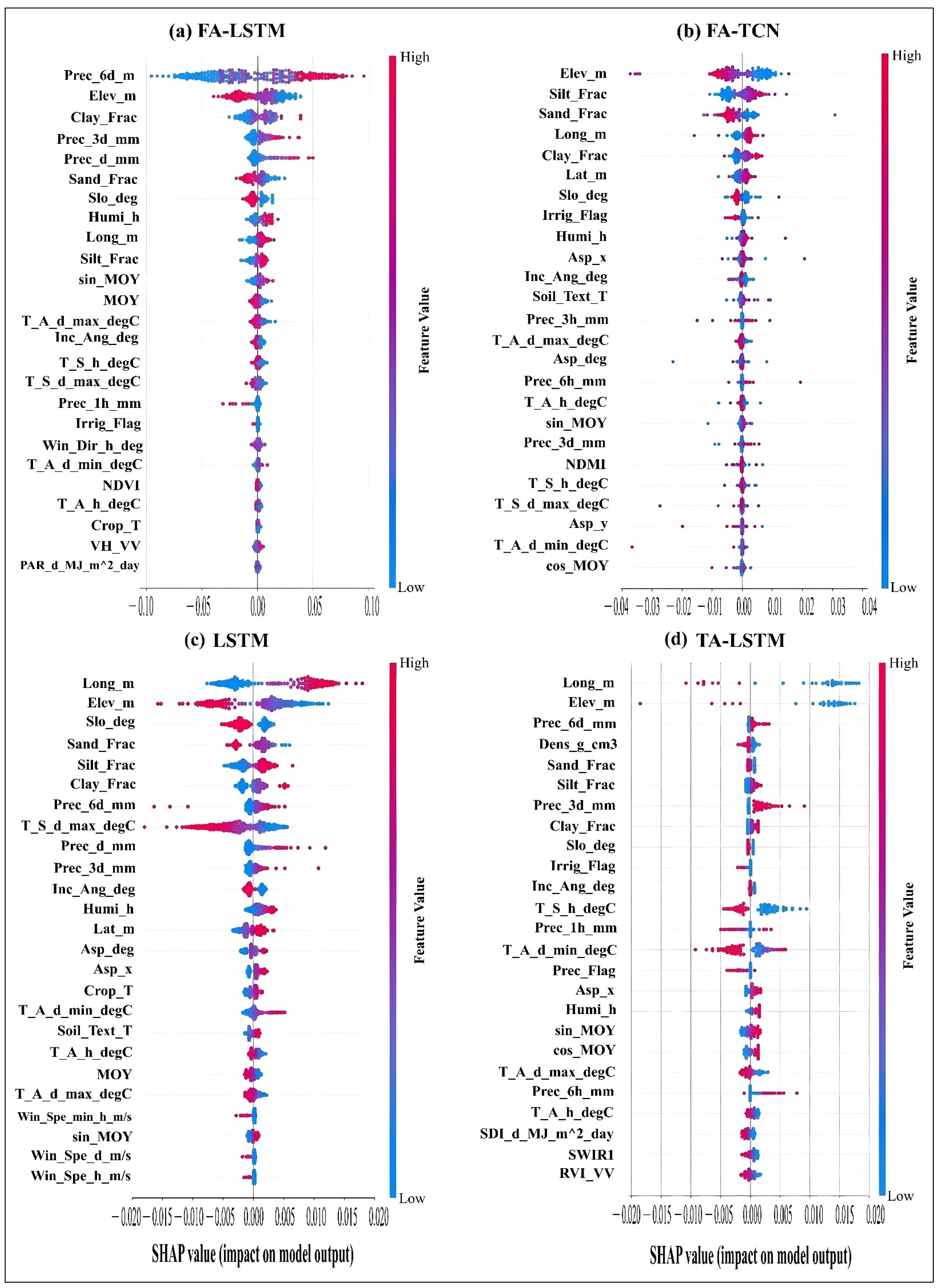
Figure A2.
SHAP beeswarm plots for FTA-LSTM, FTA-TCN, TA-TCN, and TCN illustrate the direction and magnitude of each top 30 feature influence on the target variable (SSM). Each point represents one validation sample. The x-axis is the SHAP value as a contribution to predicted SSM, and the color represents the feature values, with higher values in red and lower values in blue. Wider spreads indicate stronger and/or more variable influence, while asymmetric color patterns indicate directionality in how a feature shifts SSM predictions. Positive/negative SHAP values indicate a positive/negative contribution.
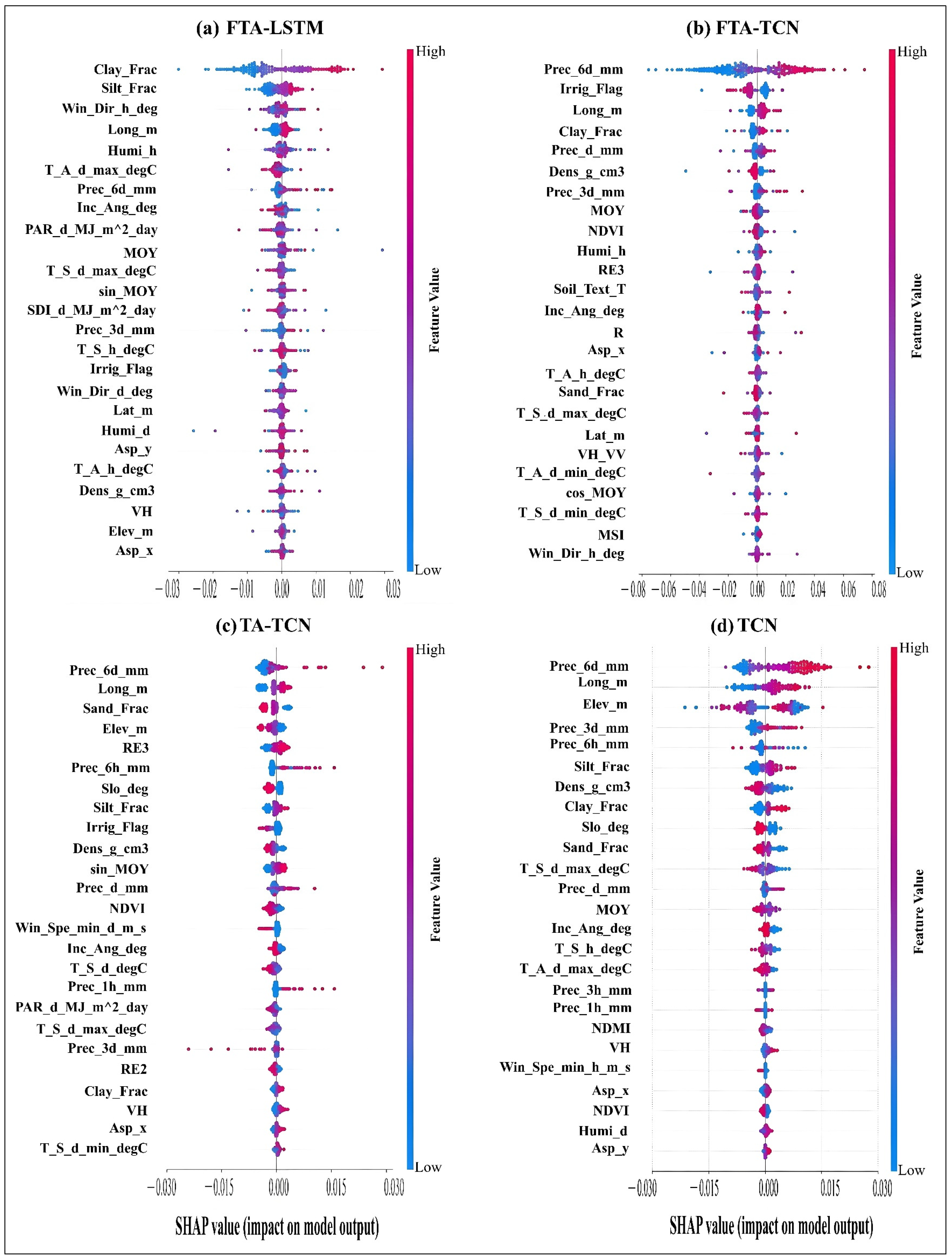
References
- Li, M.; Yan, Y. Comparative Analysis of Machine-Learning Models for Soil Moisture Estimation Using High-Resolution Remote-Sensing Data. Land 2024, 13, 1331. [Google Scholar] [CrossRef] [Scilit]
- Singh, A.; Gaurav, K. Deep Learning and Data Fusion to Estimate Surface Soil Moisture from Multi-Sensor Satellite Images. Sci. Rep. 2023, 13, 2251. [Google Scholar] [CrossRef] [Scilit] [PubMed]
- Celik, M.F.; Isik, M.S.; Yuzugullu, O.; Fajraoui, N.; Erten, E. Soil Moisture Prediction from Remote Sensing Images Coupled with Climate, Soil Texture and Topography via Deep Learning. Remote Sens. 2022, 14, 5584. [Google Scholar] [CrossRef] [Scilit]
- Li, X.; Liu, Y.; Fei, L. Estimation of Surface Soil Moisture from Multi-Source Remote Sensing Data Based on Deep Learning Model. In Proceedings of the 2023 5th International Conference on Artificial Intelligence and Computer Applications (ICAICA), Dalian, China, 28–30 November 2023; pp. 881–886. [Google Scholar]
- Wang, Y.; Shi, L.; Hu, Y.; Hu, X.; Song, W.; Wang, L. A Comprehensive Study of Deep Learning for Soil Moisture Prediction. Hydrol. Earth Syst. Sci. 2024, 28, 917–943. [Google Scholar] [CrossRef] [Scilit]
- Moore, K.R.; Lychuk, T.; Mcnairn, H.; Geng, X.; Chipanshi, A.; Ojo, E.R.; Lapen, D.; Powers, J.; Halstead, A.; Gottfried, K.; et al. Collection: Datasets from Real-Time In-Situ Soil Monitoring for Agriculture 2025. IEEE Data Descr. 2025, 2, 433–440. [Google Scholar] [CrossRef] [Scilit]
- Lee, S.-J.; Choi, C.; Kim, J.; Choi, M.; Cho, J.; Lee, Y. Estimation of High-Resolution Soil Moisture in Canadian Croplands Using Deep Neural Network with Sentinel-1 and Sentinel-2 Images. Remote Sens. 2023, 15, 4063. [Google Scholar] [CrossRef] [Scilit]
- Nativel, S.; Ayari, E.; Rodriguez-Fernandez, N.; Baghdadi, N.; Madelon, R.; Albergel, C.; Zribi, M. Hybrid Methodology Using Sentinel-1/Sentinel-2 for Soil Moisture Estimation. Remote Sens. 2022, 14, 2434. [Google Scholar] [CrossRef] [Scilit]
- Teixeira, A.C.; Bakon, M.; Lopes, D.; Cunha, A.; Sousa, J.J. A Systematic Review on Soil Moisture Estimation Using Remote Sensing Data for Agricultural Applications. Sci. Remote Sens. 2025, 12, 100328. [Google Scholar] [CrossRef] [Scilit]
- Lea, C.; Flynn, M.D.; Vidal, R.; Reiter, A.; Hager, G.D. Temporal Convolutional Networks for Action Segmentation and Detection. In Proceedings of the 2017 IEEE Conference on Computer Vision and Pattern Recognition (CVPR), Honolulu, HI, USA, 21–26 July 2016. [Google Scholar]
- Xu, Y.; Hu, C.; Wu, Q.; Li, Z.; Jian, S.; Chen, Y. Application of Temporal Convolutional Network for Flood Forecasting. Hydrol. Res. 2021, 52, 1455–1468. [Google Scholar] [CrossRef] [Scilit]
- Zhang, X.; Dong, F.; Chen, G.; Dai, Z. Advance Prediction of Coastal Groundwater Levels with Temporal Convolutional and Long Short-Term Memory Networks. Hydrol. Earth Syst. Sci. 2023, 27, 83–96. [Google Scholar] [CrossRef] [Scilit]
- Haider, A.; Lee, G.; Jafri, T.H.; Yoon, P.; Piao, J.; Jhang, K. Enhancing Accuracy of Groundwater Level Forecasting with Minimal Computational Complexity Using Temporal Convolutional Network. Water 2023, 15, 4041. [Google Scholar] [CrossRef] [Scilit]
- Guidotti, R.; Monreale, A.; Ruggieri, S.; Turini, F.; Pedreschi, D.; Giannotti, F. A Survey Of Methods For Explaining Black Box Models. Available online: https://arxiv.org/abs/1802.01933v3 (accessed on 1 July 2026).
- Li, Q.; Zhu, Y.; Shangguan, W.; Wang, X.; Li, L.; Yu, F. An Attention-Aware LSTM Model for Soil Moisture and Soil Temperature Prediction. Geoderma 2022, 409, 115651. [Google Scholar] [CrossRef] [Scilit]
- Ding, Y.; Zhu, Y.; Feng, J.; Zhang, P.; Cheng, Z. Interpretable Spatio-Temporal Attention LSTM Model for Flood Forecasting. Neurocomputing 2020, 403, 348–359. [Google Scholar] [CrossRef] [Scilit]
- Zhang, C.; Sheng, Z.; Zhang, C.; Wen, S. Multi-Lead-Time Short-Term Runoff Forecasting Based on Ensemble Attention Temporal Convolutional Network. Expert Syst. Appl. 2024, 243, 122935. [Google Scholar] [CrossRef] [Scilit]
- Qin, Z.; Zhang, Y.; Qin, H.; Mo, L.; Ren, P.; Zhu, S. A Temporal Convolutional Neural Network Fusion Attention Mechanism Runoff Prediction Model Based on Dynamic Decomposition Reconstruction Integration Processing. Water 2024, 16, 3515. [Google Scholar] [CrossRef] [Scilit]
- Lamichhane, M.; Mehan, S.; Mankin, K.R. Surface Soil Moisture Prediction Using Multimodal Remote Sensing Data Fusion and Machine Learning Algorithms in Semi-Arid Agricultural Region. Sci. Remote Sens. 2025, 12, 100255. [Google Scholar] [CrossRef] [Scilit]
- Ojo, E.R.; Bullock, P.R.; L’Heureux, J.; Powers, J.; McNairn, H.; Pacheco, A. Calibration and Evaluation of a Frequency Domain Reflectometry Sensor for Real-Time Soil Moisture Monitoring. Vadose Zone J. 2015, 14, vzj2014.08.0114. [Google Scholar] [CrossRef] [Scilit]
- Pacheco, A.; L’Heureux, J.; McNairn, H.; Powers, J.; Howard, A.; Geng, X.; Rollin, P. Real-Time In-Situ Soil Monitoring for Agriculture (RISMA) Network Metadata; Agriculture and Agri-Food Canada (AAFC): Ottawa, ON, Canada, 2019.
- McNairn, H.; Gottfried, K.; Powers, J. SMAPVEX16 Manitoba Core-Based In Situ Soil Moisture Data, Version 1; NASA National Snow and Ice Data Center Distributed Active Archive Center: Boulder, CO, USA, 2018. [Google Scholar] [CrossRef]
- Bland, J.M.; Altman, D.G. Statistical Methods for Assessing Agreement between Two Methods of Clinical Measurement. Lancet 1986, 1, 307–310. [Google Scholar] [CrossRef] [Scilit] [PubMed]
- Palmisano, D.; Mattia, F.; Balenzano, A.; Satalino, G.; Pierdicca, N.; Guarnieri, A.V.M. Sentinel-1 Sensitivity to Soil Moisture at High Incidence Angle and the Impact on Retrieval Over Seasonal Crops. IEEE Trans. Geosci. Remote Sens. 2021, 59, 7308–7321. [Google Scholar] [CrossRef] [Scilit]
- Fernández, M.; Peter, H.; Arnold, D.; Duan, B.; Simons, W.; Wermuth, M.; Hackel, S.; Fernández, J.; Jäggi, A.; Hugentobler, U.; et al. Copernicus Sentinel–1 POD Reprocessing Campaign. Adv. Space Res. 2022, 70, 249–267. [Google Scholar] [CrossRef] [Scilit]
- Filipponi, F. Sentinel-1 GRD Preprocessing Workflow. Proceedings 2019, 18, 11. [Google Scholar] [CrossRef] [Scilit]
- Simonsen, N.; Duan, Z. Development of a Deep Learning-Based Method for Estimating Surface Soil Moisture at High Spatial Resolution from Sentinel-1 Satellite Data. Master’s Thesis, Lund University, Lund, Sweden, 2021. [Google Scholar]
- Mullissa, A.; Vollrath, A.; Odongo-Braun, C.; Slagter, B.; Balling, J.; Gou, Y.; Gorelick, N.; Reiche, J. Sentinel-1 SAR Backscatter Analysis Ready Data Preparation in Google Earth Engine. Remote Sens. 2021, 13, 1954. [Google Scholar] [CrossRef] [Scilit]
- Desai, G.T.; Gaikwad, A.N. Soil Moisture Estimation Using Ground Scatterometer and Sentinel-1 Data. Bull. Electr. Eng. Inform. 2024, 13, 1707–1717. [Google Scholar] [CrossRef] [Scilit]
- Hu, X.; Li, L.; Huang, J.; Zeng, Y.; Zhang, S.; Su, Y.; Hong, Y.; Hong, Z. Radar Vegetation Indices for Monitoring Surface Vegetation: Developments, Challenges, and Trends. Sci. Total Environ. 2024, 945, 173974. [Google Scholar] [CrossRef] [Scilit] [PubMed]
- Bulut, Ü.; Mohammadi, B.; Duan, Z. Estimation of Surface Soil Moisture from Sentinel-1 Synthetic Aperture Radar Imagery Using Machine Learning Method. Remote Sens. Appl. Soc. Environ. 2024, 36, 101369. [Google Scholar] [CrossRef] [Scilit]
- Ju, J.; Zhou, Q.; Freitag, B.; Roy, D.P.; Zhang, H.K.; Sridhar, M.; Mandel, J.; Arab, S.; Schmidt, G.; Crawford, C.J.; et al. The Harmonized Landsat and Sentinel-2 Version 2.0 Surface Reflectance Dataset. Remote Sens. Environ. 2025, 324, 114723. [Google Scholar] [CrossRef] [Scilit]
- Xiong, Y.; Guo, S.; Chen, J.; Deng, X.; Sun, L.; Zheng, X.; Xu, W. Improved SRGAN for Remote Sensing Image Super-Resolution Across Locations and Sensors. Remote Sens. 2020, 12, 1263. [Google Scholar] [CrossRef] [Scilit]
- Cai, Z.; Jönsson, P.; Jin, H.; Eklundh, L. Performance of Smoothing Methods for Reconstructing NDVI Time-Series and Estimating Vegetation Phenology from MODIS Data. Remote Sens. 2017, 9, 1271. [Google Scholar] [CrossRef] [Scilit]
- Agriculture and Agri-Food Canada. Annual Crop Inventory—Open Government Portal. Available online: https://open.canada.ca/data/en/dataset/ba2645d5-4458-414d-b196-6303ac06c1c9 (accessed on 3 July 2025).
- MacDonald, H.; McKenney, D.W.; Pedlar, J.; Lawrence, K.; de Boer, K.; Hutchinson, M.F. Spatial Datasets of 30-Year (1991–2020) Average Monthly Total Precipitation and Minimum/Maximum Temperature for Canada and the United States. Data Brief 2024, 55, 110561. [Google Scholar] [CrossRef] [Scilit] [PubMed]
- Agriculture and Agri-Food Canada. Annual Reports. Available online: https://mbdiversificationcentres.ca/annual-reports-2/ (accessed on 11 November 2025).
- Lipton, Z.C.; Kale, D.C.; Wetzel, R. Modeling Missing Data in Clinical Time Series with RNNs. arXiv 2016, arXiv:1606.04130. [Google Scholar]
- Liu, J.; Hao, Z.; Ding, J.; Zhang, Y.; Miao, Z.; Zheng, Y.; Alimu, A.; Cheng, H.; Li, X. Ensemble Machine-Learning-Based Framework for Estimating Surface Soil Moisture Using Sentinel-1/2 Data: A Case Study of an Arid Oasis in China. Land 2024, 13, 1635. [Google Scholar] [CrossRef] [Scilit]
- Massey, F.J. The Kolmogorov-Smirnov Test for Goodness of Fit. J. Am. Stat. Assoc. 1951, 46, 68–78. [Google Scholar] [CrossRef] [Scilit]
- Dowd, C. A New ECDF Two-Sample Test Statistic. arXiv 2020, arXiv:2007.01360. [Google Scholar]
- Ben Shachar, M.; Lüdecke, D.; Makowski, D. Effectsize: Estimation of Effect Size Indices and Standardized Parameters. J. Open Source Softw. 2020, 5, 2815. [Google Scholar] [CrossRef] [Scilit]
- Gopali, S.; Abri, F.; Siami-Namini, S.; Namin, A.S. A Comparison of TCN and LSTM Models in Detecting Anomalies in Time Series Data. In Proceedings of the 2021 IEEE International Conference on Big Data (Big Data), Orlando, FL, USA, 15–18 December 2021; pp. 2415–2420. [Google Scholar]
- Wang, Q.; You, Y.; Yang, H.; Xu, R.; Zhang, H.K.; Lu, P.; Tong, X. A TCN-Transformer Parallel Model for Reconstruction of a Global, Daily, Spatially Seamless FY-3B Soil Moisture Dataset. Remote Sens. Environ. 2025, 328, 114841. [Google Scholar] [CrossRef] [Scilit]
- Akiba, T.; Sano, S.; Yanase, T.; Ohta, T.; Koyama, M. Optuna: A Next-Generation Hyperparameter Optimization Framework. arXiv 2019, arXiv:1907.10902. [Google Scholar]
- Chai, T.; Draxler, R.R. Root Mean Square Error (RMSE) or Mean Absolute Error (MAE)?—Arguments against Avoiding RMSE in the Literature. Geosci. Model Dev. 2014, 7, 1247–1250. [Google Scholar] [CrossRef] [Scilit]
- Paraschakis, K.; Castellani, A.; Borboudakis, G.; Tsamardinos, I. Confidence Interval Estimation of Predictive Performance in the Context of AutoML. arXiv 2024, arXiv:2406.08099. [Google Scholar]
- Cai, B.; Luo, Y.; Guo, X.; Pellegrini, F.; Pang, M.; de Moor, C.; Shen, C.; Charu, V.; Tian, L. Bootstrapping the Cross-Validation Estimate. Available online: https://arxiv.org/abs/2307.00260v2 (accessed on 30 June 2026).
- Lundberg, S.; Lee, S.-I. A Unified Approach to Interpreting Model Predictions 2017. In Advances in Neural Information Processing Systems 30; Curran Associates, Inc.: New York, NY, USA, 2017. [Google Scholar] [CrossRef] [Scilit] [PubMed]
- Kumar, I.E.; Venkatasubramanian, S.; Scheidegger, C.; Friedler, S. Problems with Shapley-Value-Based Explanations as Feature Importance Measures. arXiv 2020, arXiv:2002.11097. [Google Scholar]
- Jain, S.; Wallace, B.C. Attention Is Not Explanation. In Proceedings of the 2019 Conference of the North American Chapter of the Association for Computational Linguistics: Human Language Technologies; Volume 1 (Long and Short Papers); Burstein, J., Doran, C., Solorio, T., Eds.; Association for Computational Linguistics: Minneapolis, MN, USA, 2019; pp. 3543–3556. [Google Scholar]
- De Lannoy, G.J.M.; Koster, R.D.; Reichle, R.H.; Mahanama, S.P.P.; Liu, Q. An Updated Treatment of Soil Texture and Associated Hydraulic Properties in a Global Land Modeling System. J. Adv. Model. Earth Syst. 2014, 6, 957–979. [Google Scholar] [CrossRef] [Scilit]
- Cavieres, J.; Karkulik, M. Efficient Estimation for a Smoothing Thin Plate Spline in a Two-Dimensional Space. arXiv 2024, arXiv:2404.01902. [Google Scholar]
- Shi, C.; Zhang, Z.; Wang, B.; Zhang, W.; Yi, Y. Disentangling Vegetation Water Content and Surface Soil Moisture from Sentinel-1 Sar Time Series Through Asynchronous Convolutional Neural Network. In Proceedings of the IGARSS 2024 IEEE International Geoscience and Remote Sensing Symposium, Athens, Greece, 7–12 July 2024; pp. 1474–1477. [Google Scholar]
- Claverie, M.; Ju, J.; Masek, J.G.; Dungan, J.L.; Vermote, E.F.; Roger, J.-C.; Skakun, S.V.; Justice, C. The Harmonized Landsat and Sentinel-2 Surface Reflectance Data Set. Remote Sens. Environ. 2018, 219, 145–161. [Google Scholar] [CrossRef] [Scilit]
- Bai, S.; Kolter, J.Z.; Koltun, V. An Empirical Evaluation of Generic Convolutional and Recurrent Networks for Sequence Modeling. arXiv 2018, arXiv:1803.01271. [Google Scholar]
- Azedou, A.; Amine, A.; Lahssini, S.; Osterman, G.; Arboleda-Zapata, M.; Cosh, M.; Kisekka, I. Ensemble Deep Learning towards High-Resolution Soil-Moisture Mapping for Enhanced Water Management in California’s Central Valley. Environ. Model. Softw. 2026, 197, 106824. [Google Scholar] [CrossRef] [Scilit]
- Rahmati, M.; Balenzano, A.; Bechtold, M.; Brocca, L.; Fluhrer, A.; Jagdhuber, T.; Karamvasis, K.; Mengen, D.; Reichle, R.H.; Kim, S.; et al. Soil Moisture Retrieval from Sentinel-1: Lessons Learned after More than a Decade in Orbit. Remote Sens. Environ. 2026, 333, 115146. [Google Scholar] [CrossRef] [Scilit]
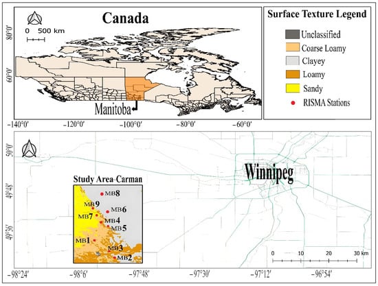
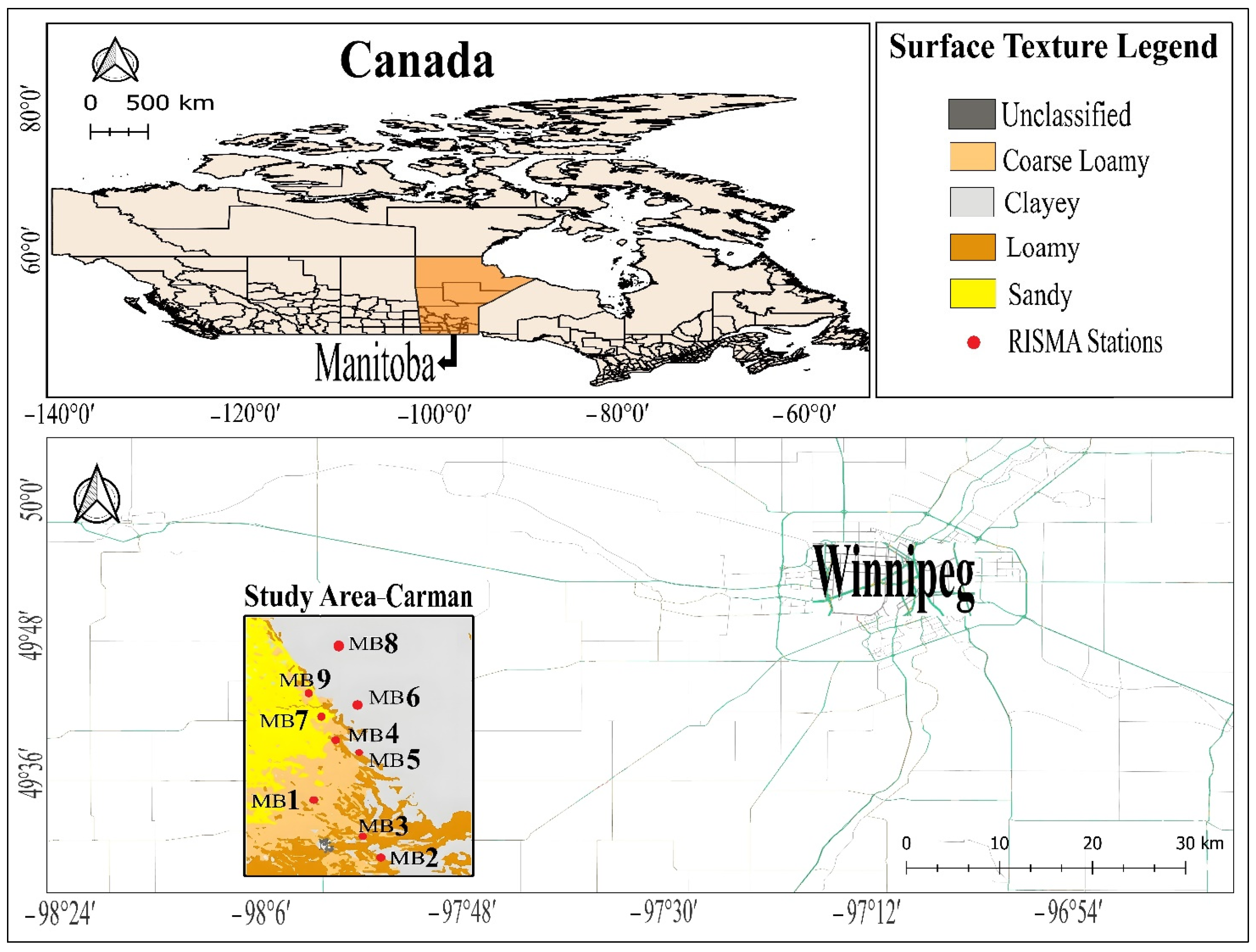
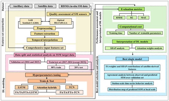
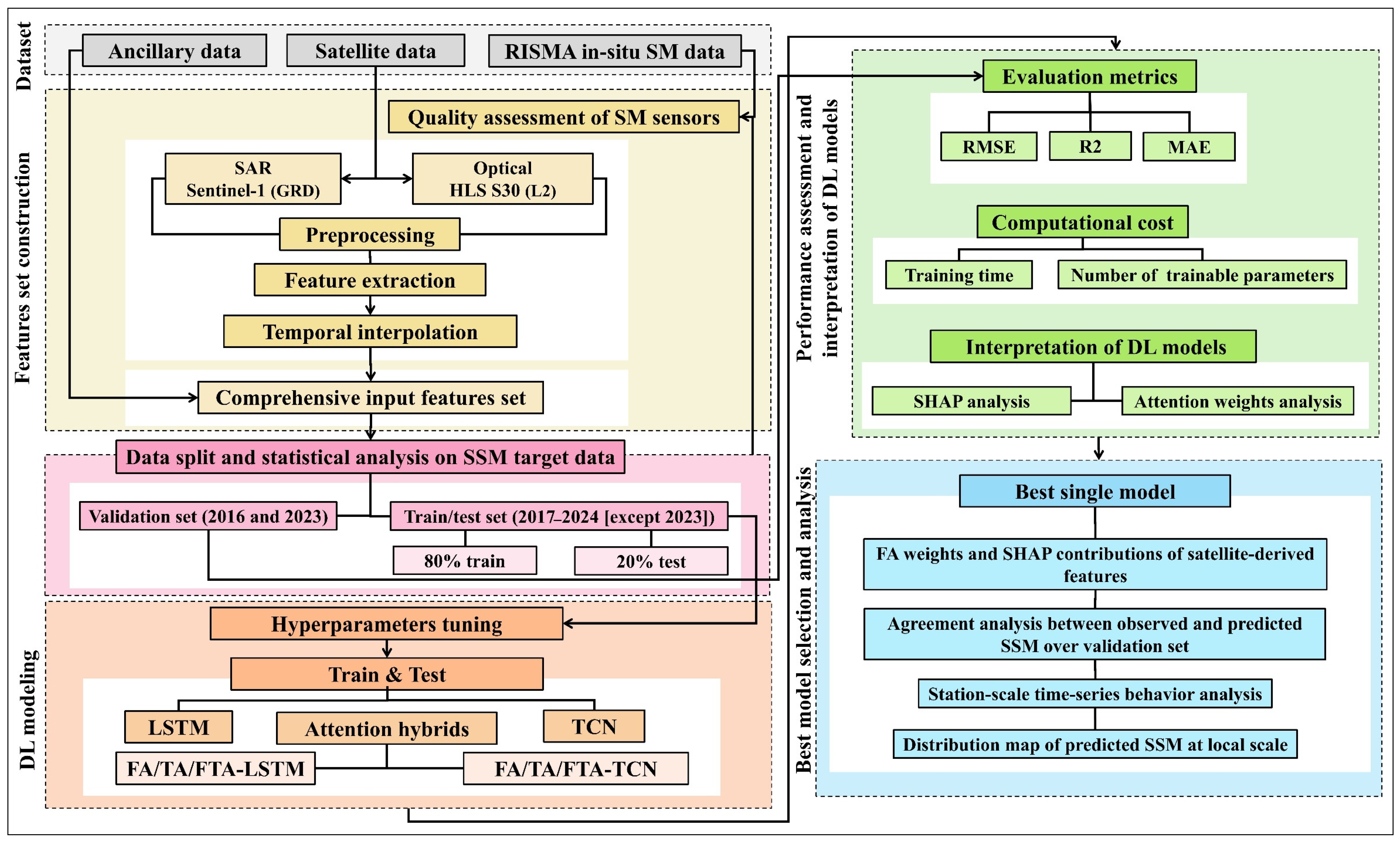
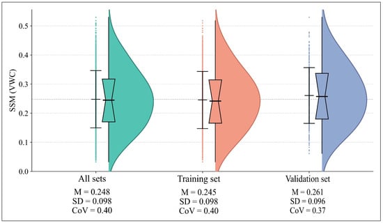
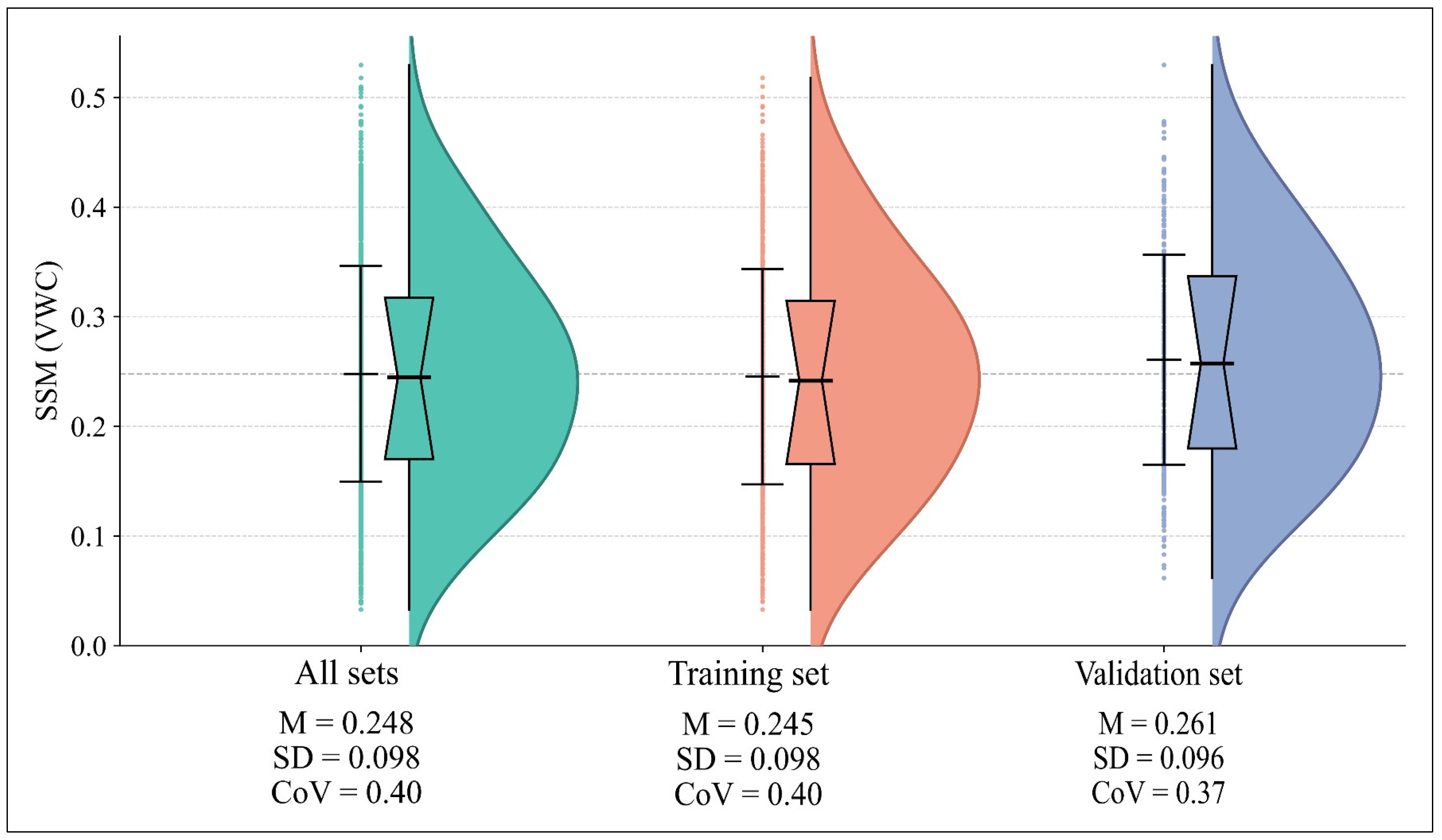
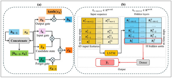
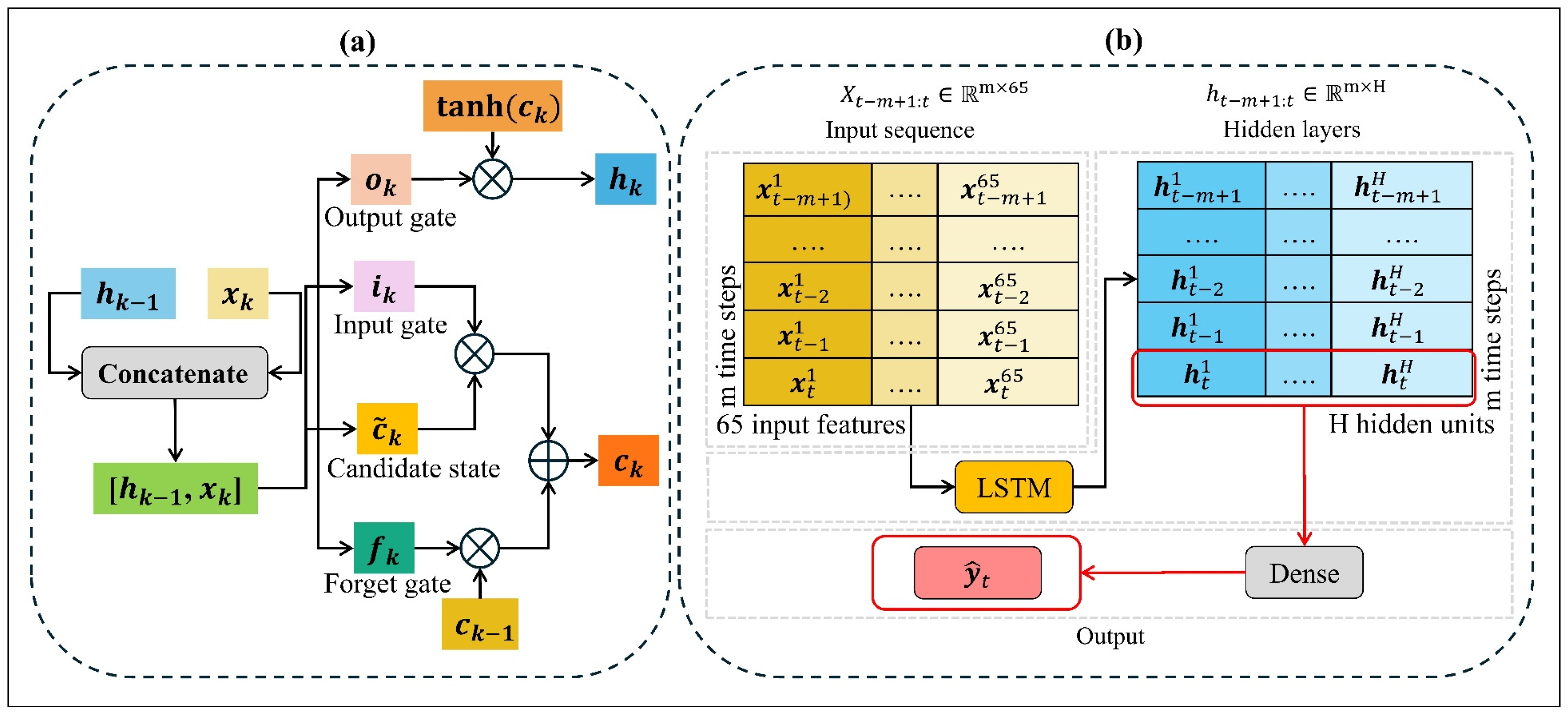
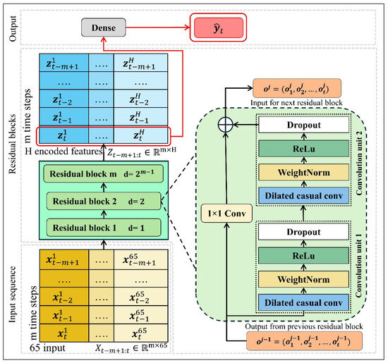
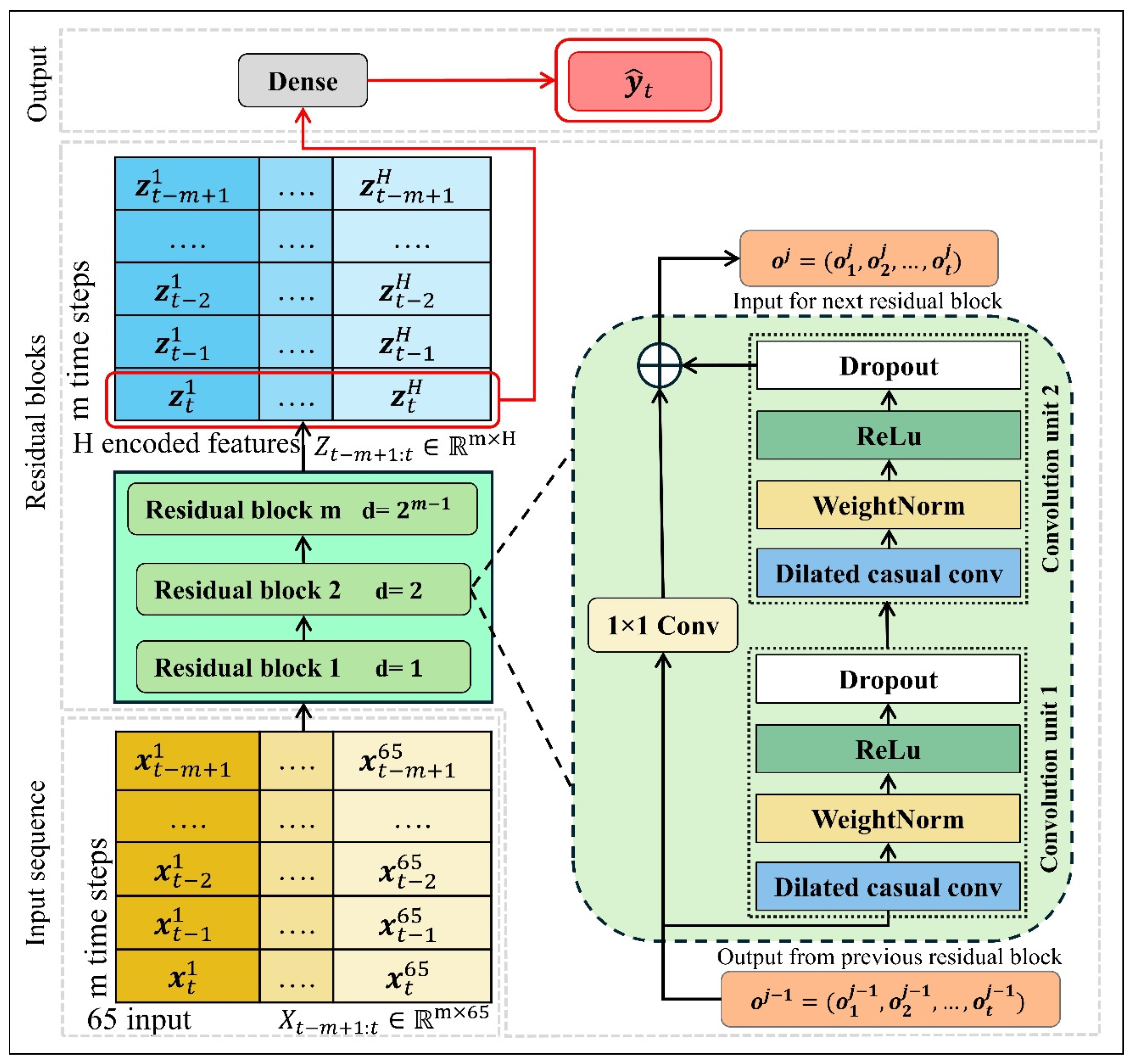
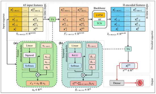
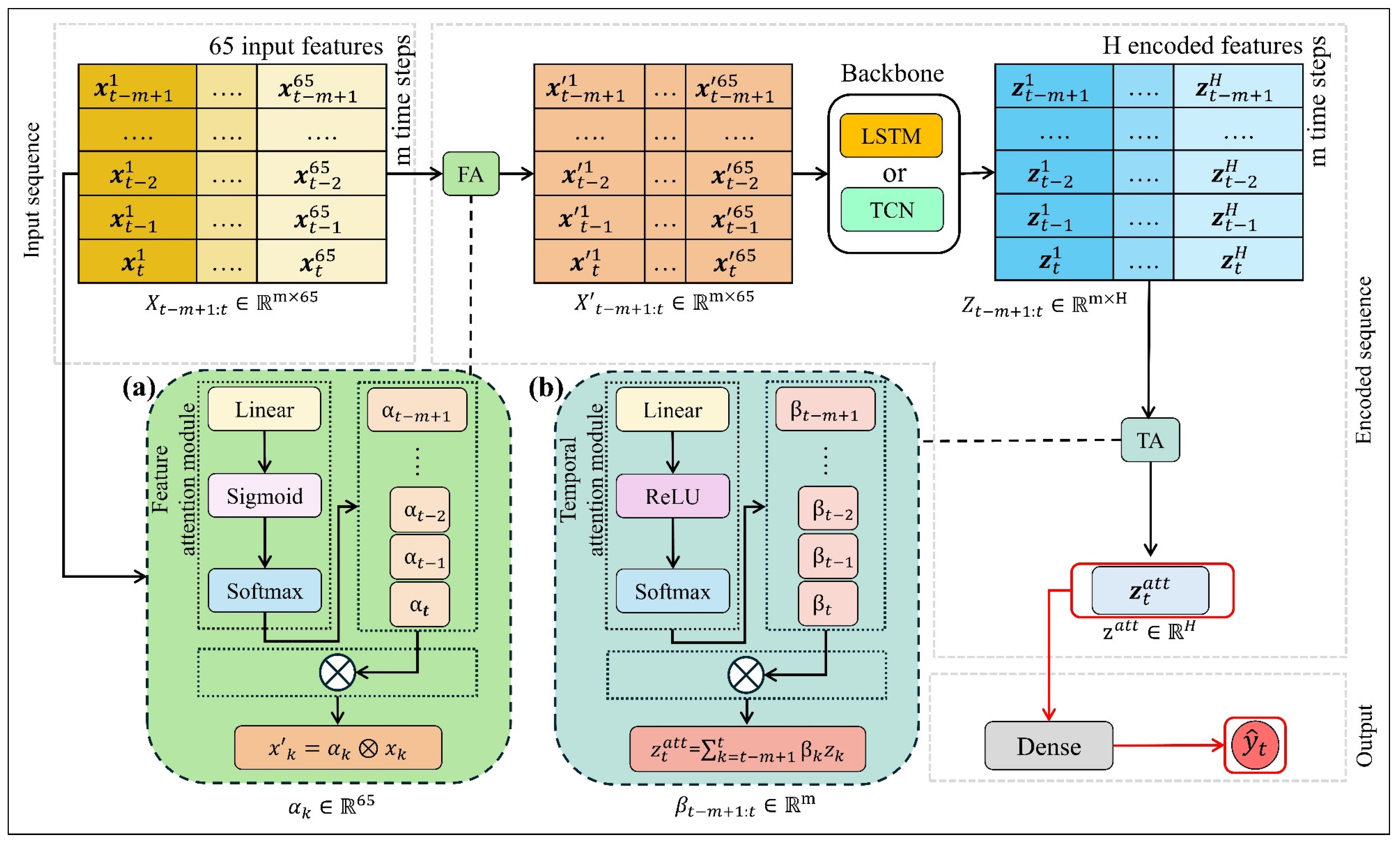
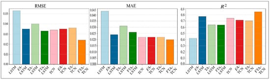
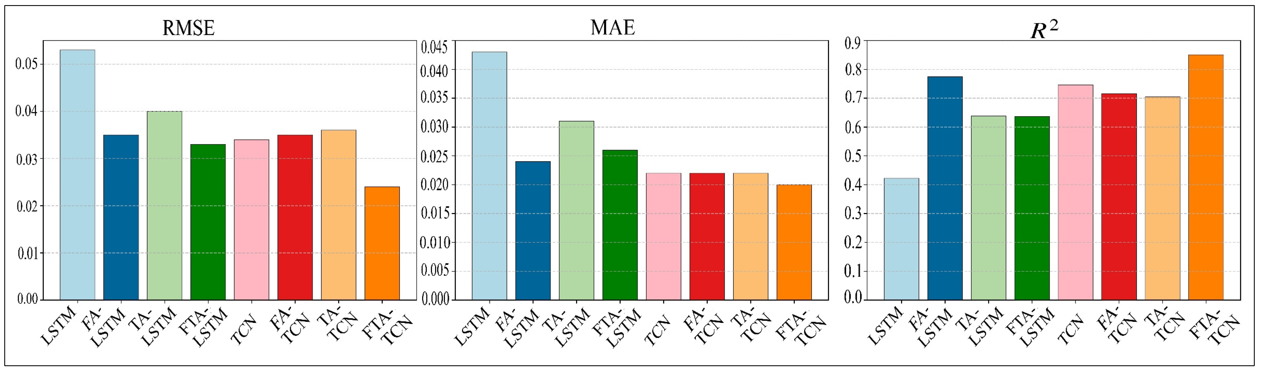
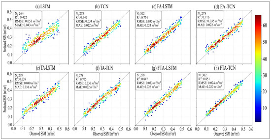
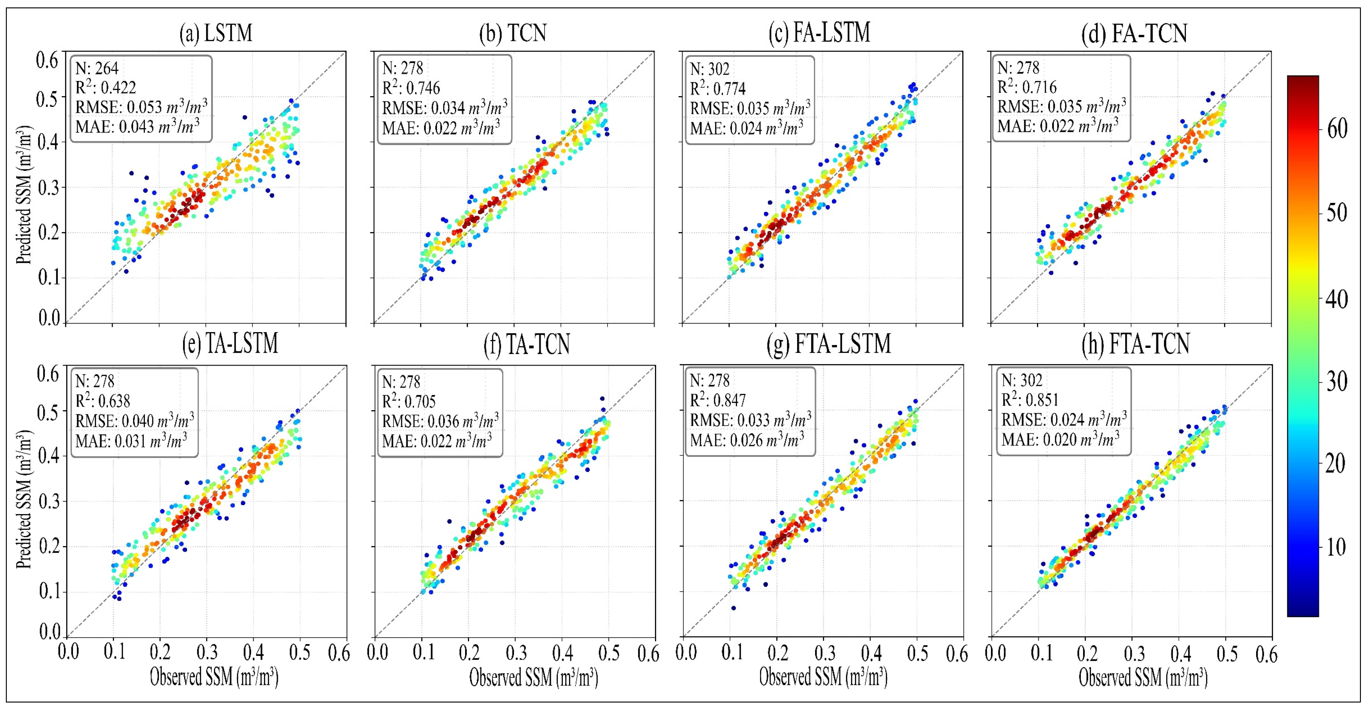
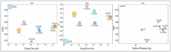
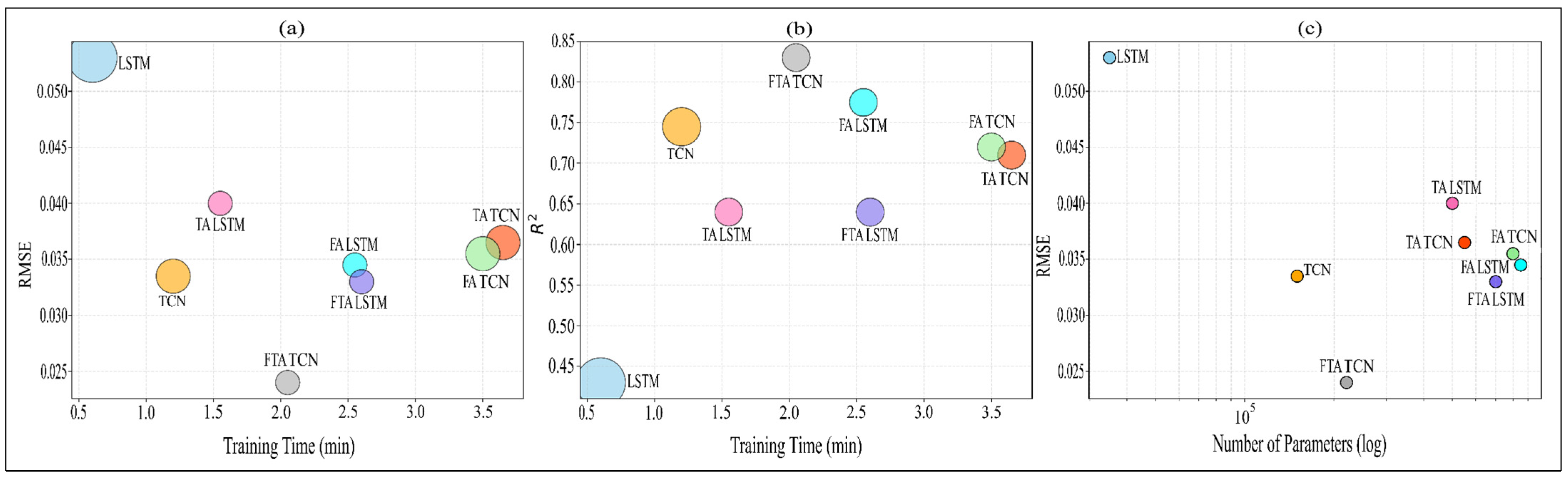
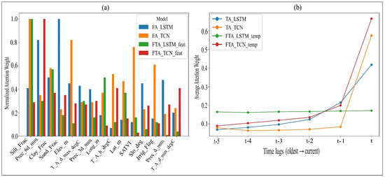
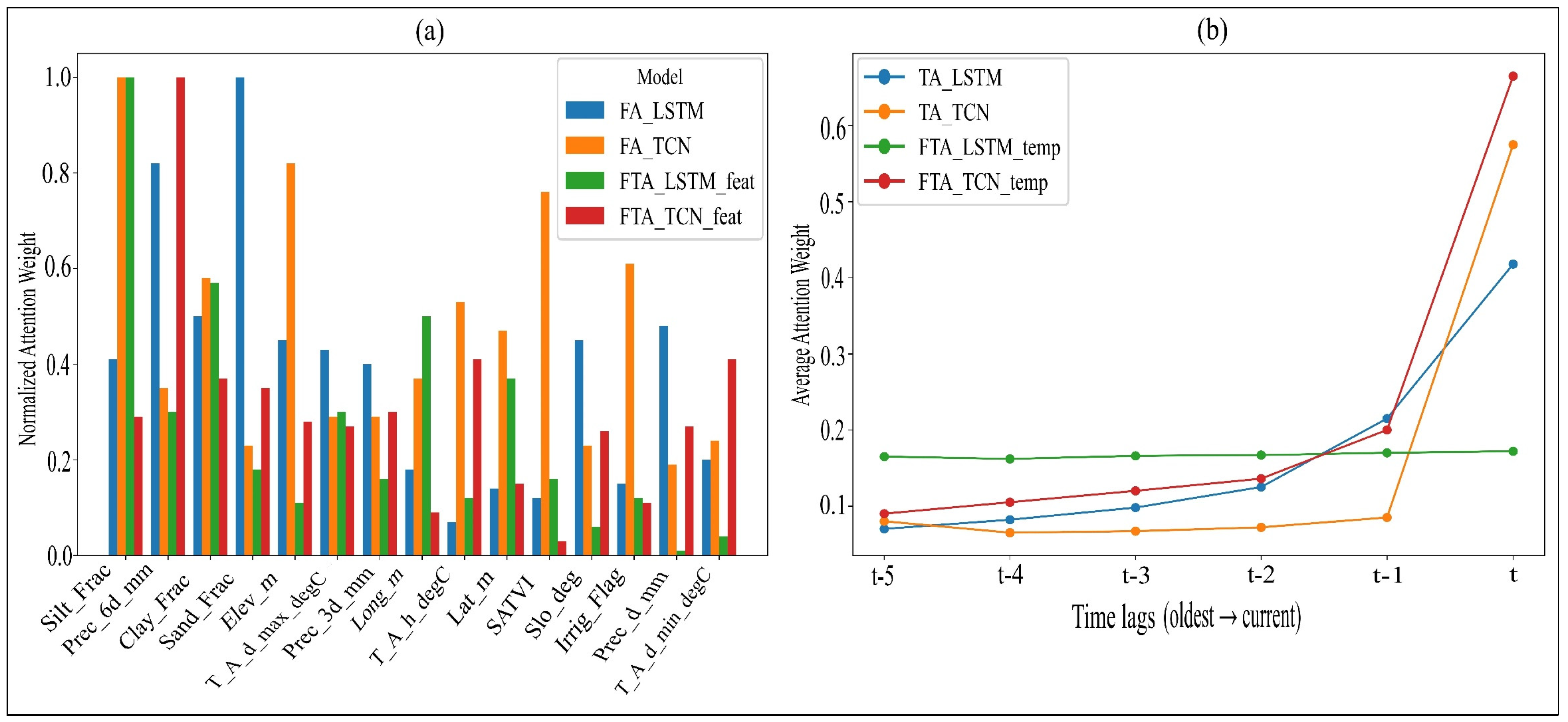
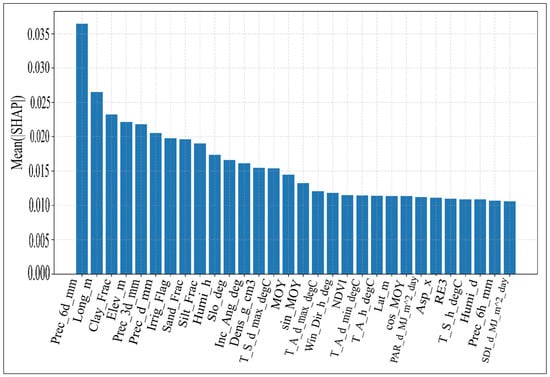
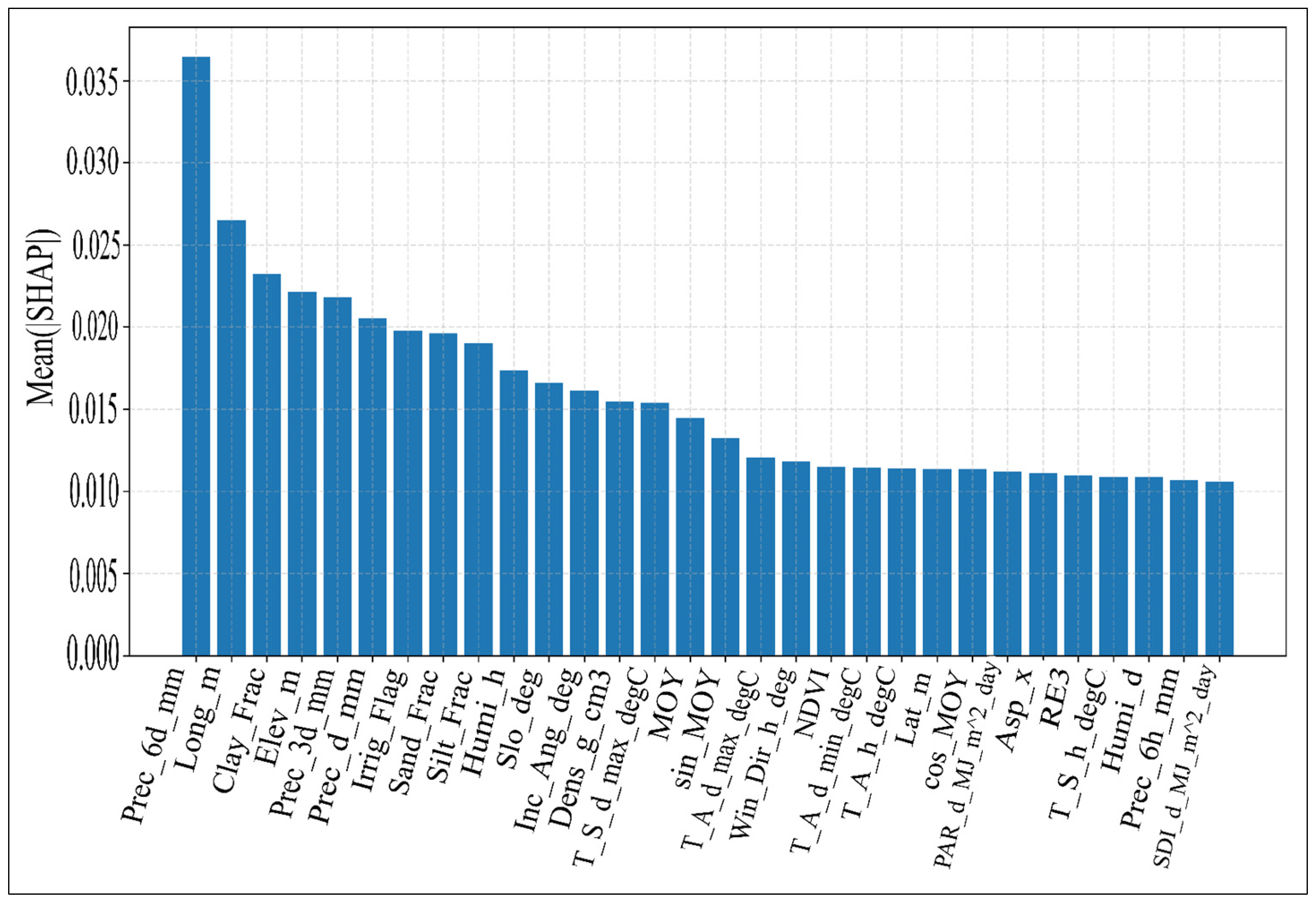
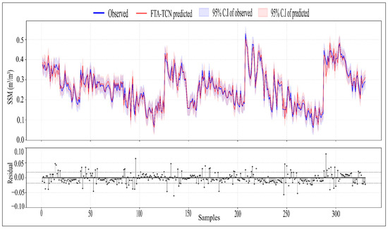
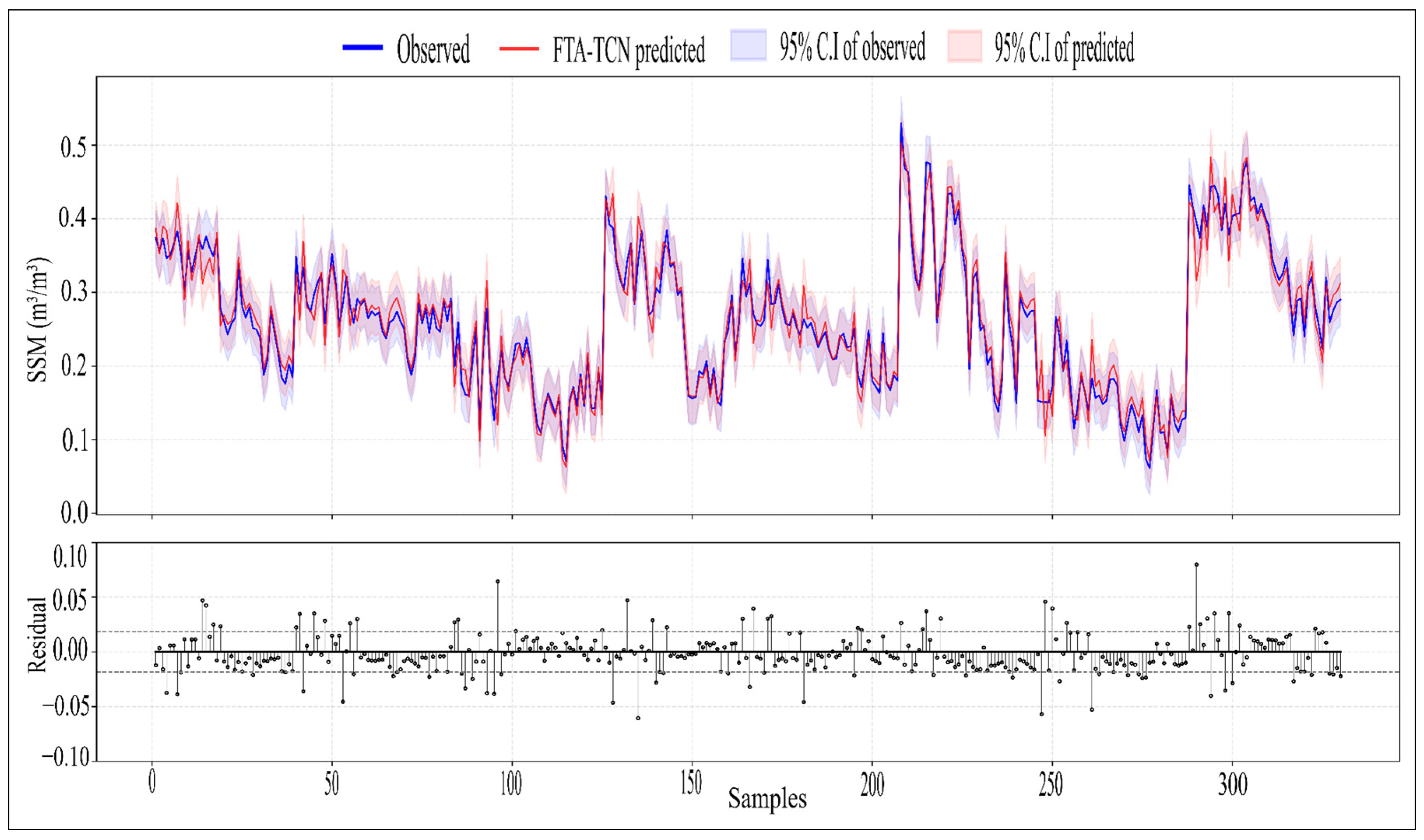
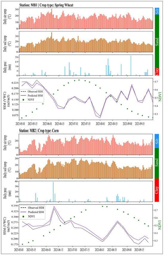
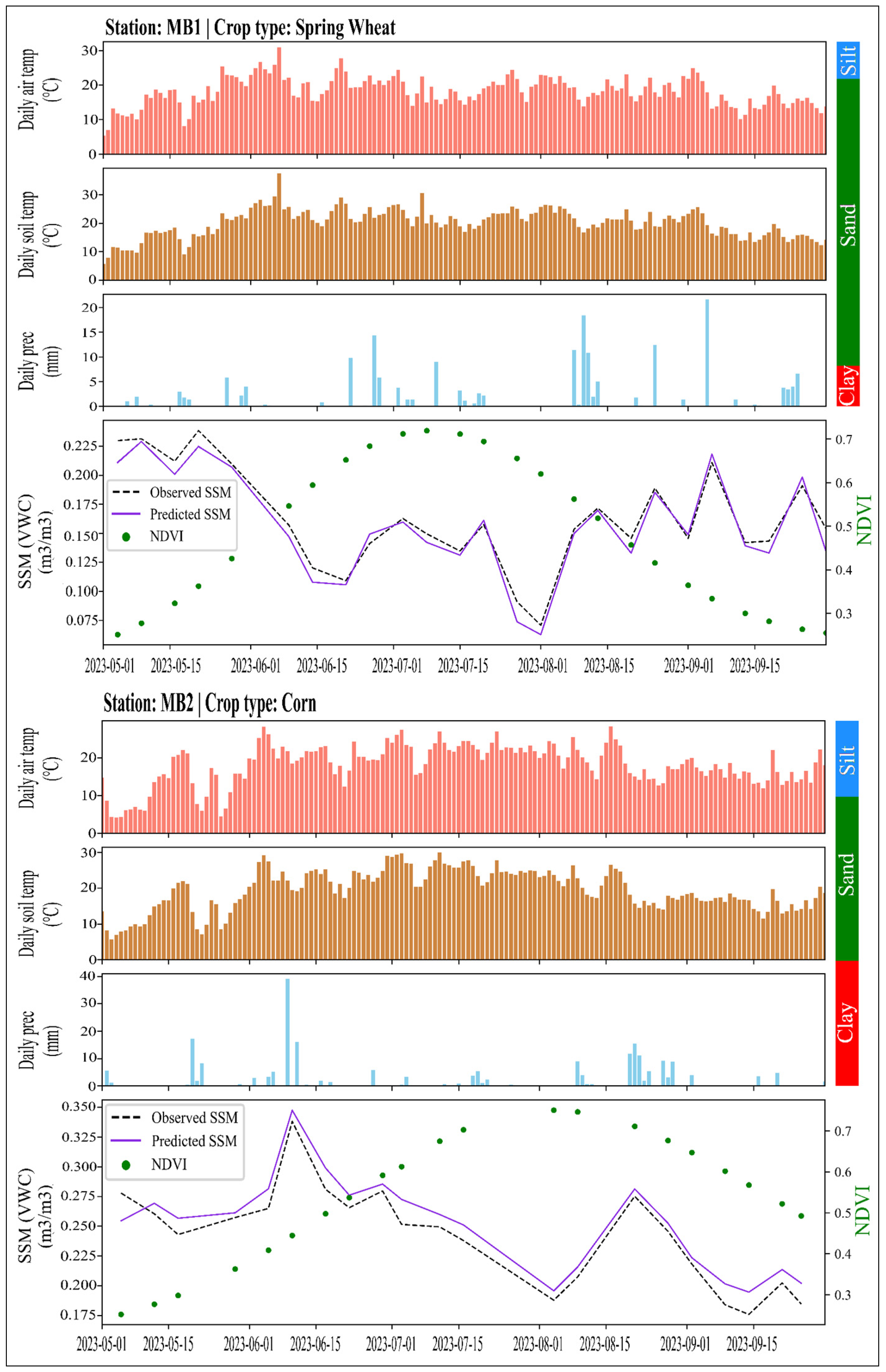
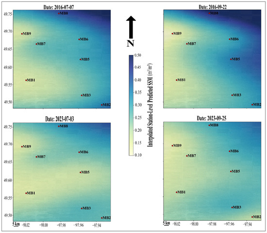
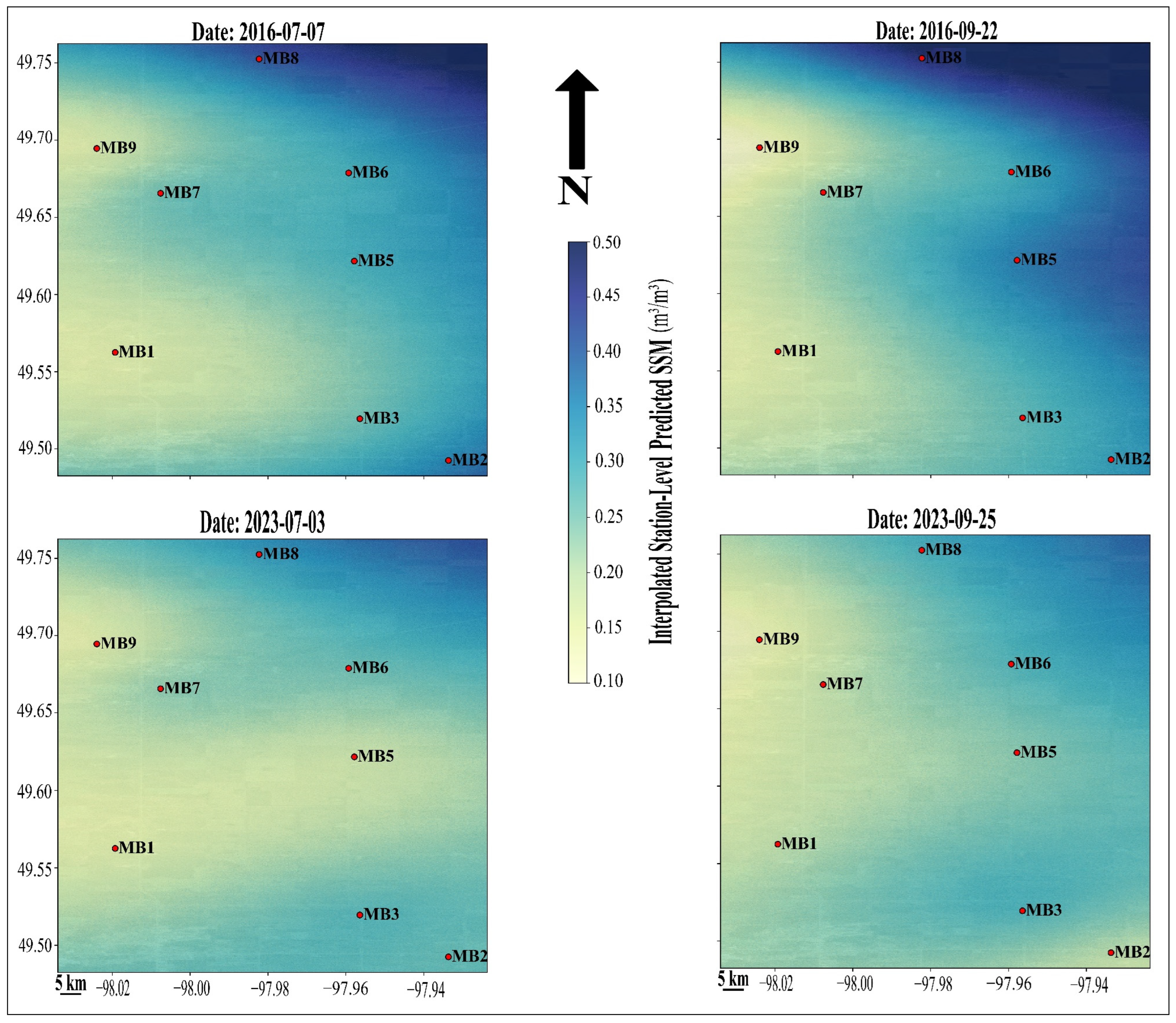

Disclaimer/Publisher’s Note: The statements, opinions and data contained in all publications are solely those of the individual author(s) and contributor(s) and not of MDPI and/or the editor(s). MDPI and/or the editor(s) disclaim responsibility for any injury to people or property resulting from any ideas, methods, instructions or products referred to in the content. |
© 2026 by the authors. Licensee MDPI, Basel, Switzerland. This article is an open access article distributed under the terms and conditions of the Creative Commons Attribution (CC BY) license.