


Highlights
What are the main findings?
- Frame-wise spatial deformable convolution is introduced to adaptively compensate for inter-frame sub-pixel jitter while reducing model parameters by approximately one quarter.
- A complex-domain frequency loss with a high-frequency weighted mask is designed to better preserve the high-frequency morphology of star spots and improve centroiding accuracy.
What are the implications of the main findings?
- The proposed method improves PSNR by ~17.8 dB and reduces centroid error to ~0.1 pixels under low-SNR conditions, significantly outperforming multi-frame stacking and BM3D.
- The proposed improvements overcome the baseline self-supervised spatiotemporal framework’s limitations in inter-frame jitter compensation and high-frequency detail preservation, enabling effective on-orbit star-sensor window images denoising without clean ground-truth data.
Abstract
In window tracking mode, stray light and detector readout noise can submerge star spot signals in star sensor images. The resulting degradation reduces centroid extraction accuracy and may even cause extraction failure, thereby preventing precise attitude determination. This study uses the self-supervised spatiotemporal denoising model ASTERIS as the baseline. ASTERIS integrates 3D spatiotemporal inputs with a global attention mechanism for joint noise modeling, thereby providing stronger denoising and restoration capability than conventional methods such as multi-frame stacking. However, ASTERIS lacks adaptive compensation for subpixel jitter in on-orbit star images and has difficulty preserving the high-frequency morphology of star spots, affecting denoising performance and centroiding accuracy. To address these limitations, this study introduces two improvements: First, frame-by-frame spatial deformable convolution is incorporated into the decoder upsampling stage to adaptively compensate for subpixel offsets, actively suppress background noise, and lower the parameter count. Second, a complex-valued frequency domain loss with a high-frequency weighted mask is designed to jointly constrain the amplitude and phase spectra, thereby preserving high-frequency star spot details. Experimental results show that, for star images with extremely low signal-to-noise ratios, the proposed method improves the peak signal-to-noise ratio by approximately 17.8 dB and reduces the centroid localization error to approximately 0.1 pixels. This performance is substantially better than that of the original ASTERIS model, which improves the peak signal-to-noise ratio by approximately 9.5 dB and yields an error of approximately 0.4 pixels, and the multi-frame stacking method, which improves the peak signal-to-noise ratio by approximately 6.0 dB and yields an error of approximately 0.5 pixels. Under the simulated strong noise conditions considered in this study, the proposed method achieves effective centroid extraction, demonstrating its potential for on-orbit star sensor data processing. Future work will further address its engineering deployment.
1. Introduction
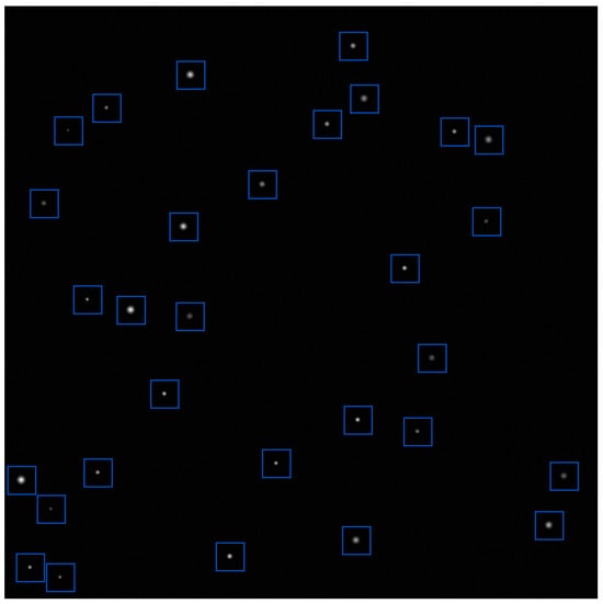
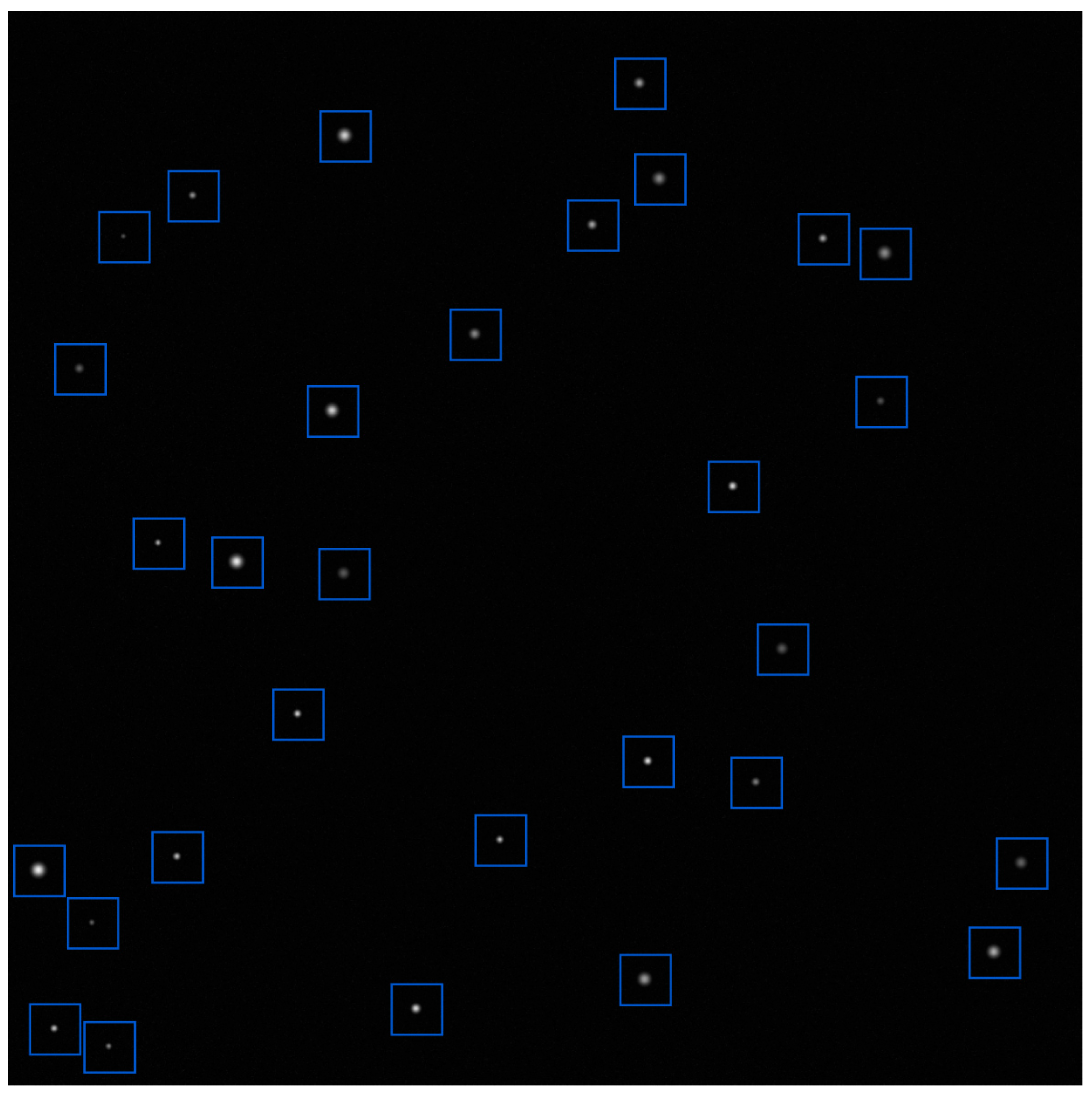
Star sensors are core optical sensors for spacecraft attitude measurement, and the attitude information provided by them directly affects the geocoding accuracy of remote sensing images and therefore influences downstream remote sensing applications. During operation, these sensors capture stellar images, extract the centroid coordinates of star spots, and determine spacecraft attitude or detect space targets through star map recognition [1,2,3]. To improve measurement accuracy and data update rates, star sensors commonly operate in window tracking mode during on-orbit observation. In this mode, the positions of known stars in the current image are predicted using the attitude information from the previous moment, and small windows centered on these predicted positions are cropped. A field-programmable gate array (FPGA) then processes each window in parallel and independently calculates the centroid of the corresponding star spot [4,5,6]. Under ideal conditions, each window contains a single star, with its centroid located at the center of the window, and the grayscale distribution follows a two-dimensional Gaussian point spread function (PSF) [7,8]. Figure 1 shows the small windows cropped from the original star map using the FPGA.
Figure 1.
Schematic diagram of small windows cropped from the original star map using the FPGA.
In actual on-orbit environments, however, the quality of window images can be strongly degraded by stray light interference from Earth airglow, direct sunlight, and internal scattering in the optical system, as well as detector readout noise and dark currents. Under such interference, star spot signals are readily submerged in background noise, and the resulting degradation reduces centroid extraction accuracy and may ultimately cause attitude determination failure [9,10].
Star sensor image interference suppression primarily involves two categories of on-orbit noise [9,10]:
The first category is detector readout noise, which refers to random fluctuations generated by electronic circuits during image sensor signal readout, including reset, amplification, and quantization noise. This noise type approximately satisfies a zero-mean-independent and identically distributed assumption in the temporal domain and appears spatially as an isotropic random shot-like pattern.
The second category is spatially non-stationary stray light, which refers to background radiation entering the optical system from the external spacecraft environment, including Earth airglow, moonlight, and internal scattering in the optical system. This interference forms a spatially nonuniform but temporally slowly varying or stable distribution on the image plane. Its typical characteristics include spatial gradients or local highlights, approximate constancy within a short time window, and spectral concentration in the low-frequency region.
In addition, platform jitter and optical distortion cause inter-frame jitters of star spots, while noise submersion hinders the recovery of high-frequency details—both of which are major challenges in star image denoising and restoration.
Among existing stray light suppression methods, multi-frame stacking remains the most widely used technical route in engineering applications [11,12]. Common implementations include mean, median, and weighted stacking [13]. Mean stacking can suppress Gaussian noise effectively, but this strategy is sensitive to outlier frames, namely abnormal observations caused by sudden and short-duration interference in a continuously acquired image sequence. Median stacking is robust to transient noise such as cosmic rays, but this strategy cannot remove spatially continuous background gradients. Weighted stacking assigns weights according to the inter-frame signal-to-noise ratio, yet the weight estimation process itself is easily disturbed by noise [14,15]. To mitigate this issue, several improved stacking strategies have recently been proposed. For example, inertial measurements are used in the inter-frame attitude correlation method to predict star spot displacements [16], thereby improving alignment accuracy, while relative attitude changes are estimated in the image autocorrelation method via inter-frame star spot correspondences to achieve an unbiased transformation [17]. These approaches reduce the sensitivity to weight estimation and enhance stacking robustness. However, they remain constrained by the inherent limitations of multi-frame stacking: they cannot suppress the mean background of spatially non-stationary stray light, and they inherently act as low-pass filters. Overall, multi-frame stacking methods share three limitations: the statistical assumptions for stray light and noise are overly idealized; adaptive compensation for subpixel jitters of star spots is limited, and high-frequency star spot details are often weakened during background suppression. These limitations may cause dim stars to be missed or photometric distortion [18,19].
Methods beyond multi-frame stacking also have clear constraints. Wavelet threshold denoising [9] suppresses noise by exploiting sparsity in the wavelet domain, and threshold selection is empirical and prone to pseudo-Gibbs artifacts. Non-local means (NLM) filtering [11] is used for image self-similarity-based weighted averaging and is effective for uniform background denoising; however, its computational complexity is high, and texture preservation remains limited. Three-dimensional block matching (BM3D) and the volumetric extension BM4D [14,15] achieve strong denoising performance through collaborative filtering of grouped blocks. However, these methods require accurate block matching, are prone to failure in star maps affected by severe stray light interference, and are difficult to deploy in real-time star sensor systems. In general, these traditional methods depend on manually designed priors, provide limited adaptive modeling of spatially non-stationary stray light and spectral aliasing between stray light and star spot signals, and often incur high computational cost. Therefore, this study uses multi-frame stacking, the most common and computationally simple engineering method, as the representative traditional baseline to evaluate the improvement provided by deep learning. The processing results of the state-of-the-art BM3D algorithm on this paper’s test dataset are also provided as a reference for comparison, as described below in Section 4.2.
Deep learning has recently provided a promising route for star map restoration. Rather than relying on manually specified priors, deep learning methods can learn restoration priors directly from image pixels and are therefore less constrained by the assumptions that limit traditional algorithms. Convolutional neural network (CNN)-based methods have shown good performance in star spot detection and centroid positioning [20,21], and Transformer architectures have further improved image restoration capability. Restormer [22] uses Multi-Dconv Head Transposed Attention (MDTA) to detect global interactions along the channel dimension and combines MDTA with a Gated-Dconv Feed-Forward Network (GDFN), thereby improving restoration quality while maintaining computational efficiency. ASTERIS [23], a state-of-the-art model, extends Restormer to 3D spatiotemporal sequences and employs self-supervised learning to improve the detection sensitivity of the James Webb Space Telescope by one magnitude, showing its strong denoising capability. In this study, we have adopted ASTERIS as the baseline because its 3D spatiotemporal self-supervised learning framework is methodologically instructive and suitable for the multi-frame stacking of star sensor window images.
Despite these advances, directly applying existing deep learning methods to star-sensor window tracking remains challenging, particularly under severe stray light interference that submerges star spots in noise. Two limitations are especially important. First, existing methods provide insufficient adaptive compensation for subpixel-level jitter of star spots. In orbit, the small inter-frame jitters in star spots prevent accurate registration and alignment of multi-frame star images and consequently degrading the denoising performance of models such as ASTERIS [23]. Additionally, ordinary convolution responds weakly to such displacements, leading to feature misalignment. Second, existing methods lack an explicit mechanism for preserving the high-frequency energy of star spots, and the star spot signal appears as a medium-to-high frequency component in the window image [24]. During training, a network may weaken star spot sharpness to obtain a smoother background, characterized by reduced peak intensity and an increased PSF diffusion radius. To address these limitations, this study introduces two improvements.
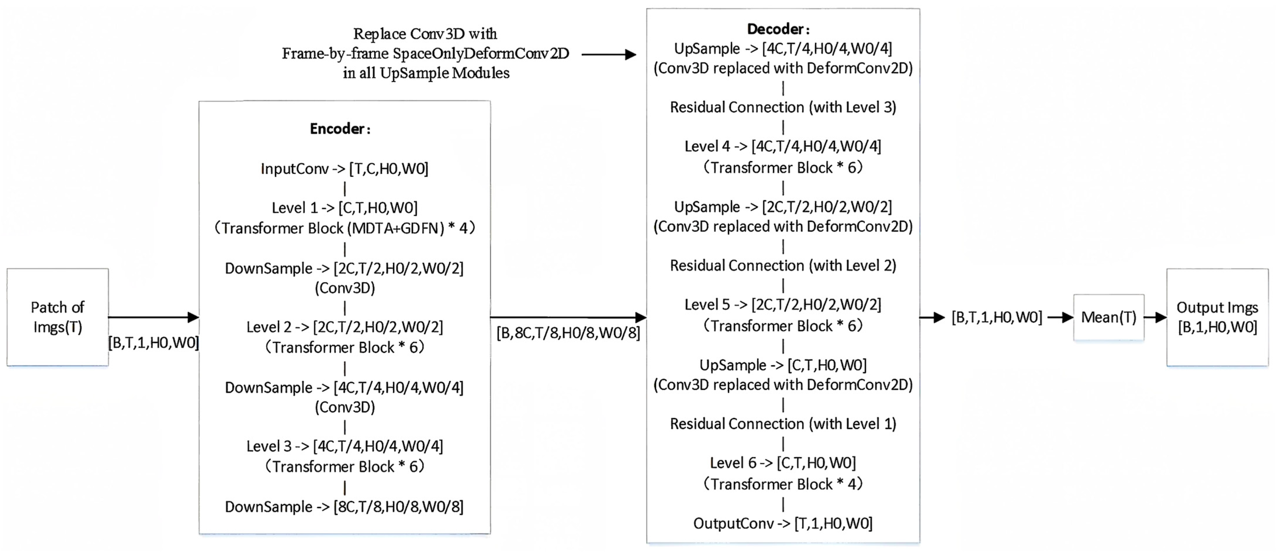
First, frame-by-frame spatial deformable convolution, hereafter referred to as deformable convolution, is incorporated into the decoder to replace standard 3D convolution. In the decoder upsampling stage, a spatial offset field is predicted independently for each frame and then used for two-dimensional deformable convolution. This design enables the sampling positions of the convolution kernel to adaptively follow the actual locations of star spots and is inspired by deformable convolution [25] and its lightweight improvement [26]. Placing deformable convolution in the upsampling stage is advantageous because high-resolution feature maps support more accurate offset estimation, and deformable convolution close to the output end can more directly correct positional errors accumulated by the encoder. The operation only compensates for displacements in the spatial dimensions and does not alter the temporal axis, which is consistent with the physical fact that star spot displacement occurs within the image plane.
Second, a frequency domain constraint is introduced into the loss function. A complex-domain frequency domain loss and a high-frequency weighted mask, hereafter referred to as the frequency domain loss constraint, are used to explicitly constrain the high-frequency components of star spots. This design draws on the structural similarity index [27] and joint wavelet–frequency domain loss [28], and strong denoising performance is obtained when the magnitude of this loss is comparable to that of the spatial domain loss. Recent methods based on diffusion models [29], implicit neural representations [30], and joint loss functions integrating frequency domain and perceptual losses [31] also support the effectiveness of frequency domain constraints.
Because noise-free ground truth star maps are difficult to obtain during on-orbit operation, self-supervised learning provides a practical training strategy. Self-supervised frameworks such as Noise2Noise [32], Noise2Void [33], and Noise2Self [34] establish the theoretical basis for training without clean targets, and CNN-based denoising methods such as DnCNN [35] and FFDNet [36] have also informed subsequent research. Both convolution-based 3D Res U-Net [21] and Transformer-based Restormer [22] can be trained within a self-supervised framework. ASTERIS adopts this self-supervised spatiotemporal denoising strategy to enhance deep space images without ground truth. With ASTERIS as the baseline, a self-supervised strategy is used to train the model with multi-frame noisy sequences acquired in the window tracking mode of star sensors.
For the two categories of on-orbit noise interference described above, traditional multi-frame stacking methods suppress zero-mean random noise by exploiting temporal redundancy. For spatially non-stationary stray light, however, stacking can only preserve the mean background and cannot improve spatial nonuniformity, even when the interference is independent between frames [11,12,13,14,15]. The effectiveness of self-supervised deep learning methods also depends on the assumption that inter-frame noise is independent and identically distributed. For interference with a nonzero mean, such as dark field or fixed pattern noise, any method based on temporal independence only cannot remove the mean component, because both stacking and self-supervised learning preserve this component.
The simulation dataset used in this study mainly contains detector readout noise and spatial random stray light interference, both of which are independently generated for each frame and have an approximately zero statistical expectation, and under these conditions, deep learning methods can fully exploit their advantages. The remainder of this paper is organized as follows: Section 2 reviews related work, and Section 3 describes the proposed method. Section 4 presents the experimental design and results, and Section 5 summarizes the study and discusses future directions.
2. Related Work
2.1. Traditional Star Image Denoising Methods
Traditional star image denoising methods can be divided into spatial domain filtering, transform domain filtering, and multi-frame stacking. Spatial domain filtering methods, including Gaussian, median, and bilateral filtering, are simple to implement but have clear limitations. In contrast, gaussian filtering blurs edges, while median filtering fails to handle gradually varying backgrounds, and bilateral filtering requires careful parameter tuning [11,12]. Transform domain filtering methods, such as DCT and wavelet threshold denoising [9], strongly depend on threshold selection and basis function matching and are prone to distortion when spectral overlap occurs [13,14]. Multi-frame stacking is the most widely used approach. Mean stacking is susceptible to outlier frames, while median stacking fails to remove spatially continuous backgrounds, and improved methods based on image autocorrelation [18] depend on the success rate of initial star spot extraction. Overall, traditional methods rely on overly idealized statistical assumptions about stray light. This dependence makes it difficult to preserve the PSF morphology of star spots while suppressing the background and can cause dim stars to be missed or grayscale distortion [19].
2.2. Deep Learning-Based Methods
Self-supervised learning: Noise2Noise demonstrates that, under zero-mean inter-frame-independent noise, training can be performed using only pairs of noisy images. The theoretical basis is as follows: for a noisy pair with the form x1 = y + n1 and x2 = y + n2, where y denotes the ground truth and n1 and n2 denote noise interference, minimizing the difference between x1 and x2 is equivalent to learning a mapping from noisy images to obtain the clean signal y. Noise2Void and Noise2Self further enable training from a single noisy image by constructing self-supervised signals through blind spot networks or pixel-masking strategies. Noise2Noise does not use temporal axis information in multi-frame sequences, whereas 3D models such as ASTERIS stack sequences into 3D tensors and use spatiotemporal self-attention to jointly model spatial details and temporal dependencies. This strategy provides stronger performance under low signal-to-noise ratios and can also reduce the influence of outlier frames in multi-frame stacking, as the grayscale distribution of an outlier frame differs substantially from that of other frames in the sequence. To minimize fitting error, the network tends to treat such frames as noise and suppress their contribution.
3D Res U-Net architecture, abbreviated as 3DRU-Net: This architecture introduces a 3D encoder–decoder structure with residual connections [21], which alleviates gradient vanishing and has been widely used in medical image segmentation and denoising. However, its convolution operations are local operators, and long-range spatiotemporal dependencies must be transmitted indirectly through repeated downsampling and upsampling. Under the operating conditions considered in this study, this limitation can cause loss of high-frequency star spot details. Static convolution kernels also assign the same spatial weights to all inputs, which makes adaptive discrimination between star spots and stray light backgrounds difficult.
Transformer architecture: Restormer [22] uses MDTA to detect global interactions along the channel dimension and combines MDTA with GDFN to improve restoration quality efficiently. MDTA transposes self-attention computation from the spatial dimension to the channel dimension, thus reducing the computational complexity from O(N2) to O(C2), where N is the number of pixels and C is the number of channels, with C much smaller than N. In contrast, ASTERIS [23] extends Restormer to 3D spatiotemporal sequences and adopts self-supervised spatiotemporal denoising. Unlike 3DRU-Net, which relies on local convolution and the indirect transmission of long-range dependencies, the Restormer-based 3D Transformer enables each spatial position to interact directly with all positions in the image through MDTA, thereby providing a global receptive field. Dynamic attention weights can also focus adaptively on star spot regions according to the input signal, and experiments show that, under low signal-to-noise ratios, ASTERIS achieves a substantially greater PSNR improvement than 3DRU-Net [23].
Deformable convolution: Deformable convolution [25] enables convolution kernels to adaptively follow target deformation by learning sampling point offsets and can compensate for subpixel displacement of star spots. These offsets are predicted from the input feature map by an additional convolutional layer. However, using 3D deformable convolution directly introduces unnecessary offsets in the temporal dimension and entails high computational overhead. Recent research [26] has explored deformable convolution placement in the decoder stage. Inspired by this strategy, we apply frame-by-frame spatial deformable 2D convolution in the upsampling stage. The experiments show that this placement is superior to applying deformable convolution in the downsampling stage, and the downsampling stage comparison is discussed below in Section 4.4.1.
3. Proposed Method
3.1. Problem Formulation
Given an input sequence of window images with a window size of H × W, the ideal grayscale distribution of the star spot follows the PSF [7], whereas the observed image is degraded by stray light and noise interference. The objective is to learn the mapping between the degraded observation and the ideal star spot signal so that a clean image can be restored.
Each noisy image frame It can therefore be regarded as the superposition of three types of signals, as shown below:
where St denotes the clean star spot signal, whose grayscale distribution approximately follows the PSF; Bt denotes spatial random stray light, which is independent between frames and has an approximately zero mean; and Nt denotes detector readout noise, which approximately satisfies a zero-mean Gaussian-independent and identically distributed assumption in the temporal sequence, as shown below:
The objective of this study is to design a trainable mapping function that takes a multi-frame sequence It as input and outputs the corresponding restored multi-frame image St.
3.2. Baseline ASTERIS Model
This study adopts ASTERIS as the backbone network [23]. The core of ASTERIS comprises a 3D Transformer encoder–decoder structure, and the input sequence is stacked into a 3D tensor X (T × H × W), processed by a 3D convolutional layer, and then fed into the MDTA module. MDTA performs self-attention along the channel dimension, enabling each channel to interact with all spatiotemporal positions and thereby providing a global receptive field, while GDFN enhances nonlinear representations through a gating mechanism [22]. By stacking multiple Transformer blocks, the network progressively learns the mapping from noisy observations to the clean signal.
ASTERIS uses a self-supervised learning strategy in which adjacent-frame noisy image pairs serve as supervisory signals. When the noise satisfies zero-mean and inter-frame independence assumptions, learning inter-frame mappings enables the network to converge toward the denoised clean signal. The loss function jointly optimizes two spatial domain losses. L1stack is a smooth L1 loss that constrains pixel-level differences between the single-frame output and the target, thereby preserving high-frequency details and star spot edges. In contrast, L2mean is a mean squared error loss for the sequence mean image, which suppresses the accumulation of inter-frame random noise and improves the signal-to-noise ratio. These two losses provide complementary constraints.
3.3. Theoretical Advantages over Multi-Frame Stacking
Traditional multi-frame stacking linearly combines pixel values along the temporal axis, and its denoising capability is derived from temporal redundancy. This strategy has three inherent limitations: First, for spatially non-stationary backgrounds, stacking can only preserve the mean distribution and cannot improve spatial nonuniformity. Second, stacking cannot compensate for subpixel jitter of star spots, so direct stacking increases the energy diffusion radius. Third, stacking is essentially a low-pass filtering operation that weakens the high-frequency morphology of star spots. The improved ASTERIS-based deep learning method used in this study addresses these limitations through four aspects.
First, spatial information helps to adaptively smooth the spatial nonuniformity of the background. Through 3D convolution and attention mechanisms, the deep learning model learns the spatial distribution of the background within a single frame and uses a large receptive field to smooth the background adaptively. Even when the background mean is not zero, the network can use spatial context to attenuate the visual impact of the background. By contrast, multi-frame stacking fully preserves the mean background and is therefore less effective at improving the signal-to-noise ratio.
Second, deformable convolution provides adaptive compensation for subpixel jitter. By learning spatial offsets for each sampling point, deformable convolution enables the sampling grid of the convolution kernel to align actively with the center of the star spot and supports precise subpixel-level fusion.
Third, the frequency domain loss explicitly preserves the high-frequency morphology of star spots. This loss constrains the amplitude and phase spectra simultaneously and strengthens the mid- and high-frequency components through a high-frequency weighted mask. This design helps avoid excessive smoothing, whereas the low-pass characteristics of multi-frame stacking tend to weaken star spot edges.
Fourth, MDTA provides joint spatiotemporal modeling and enables each spatial position to perceive information from all temporal frames simultaneously, allowing for the network to distinguish temporally varying star spots from temporally stable backgrounds and to suppress the background spatially. The experiments shown in Section 4 verify these advantages.
3.4. Frame-by-Frame Spatial Deformable Convolution
3.4.1. Design Motivation
Deformable convolution is applied in the upsampling stage for three reasons. First, the feature maps in the upsampling stage have a higher resolution, which supports accurate prediction of subpixel offsets. Second, the decoder fuses details lost during downsampling, and deformable convolution can directly correct accumulated positional errors. Third, gradient propagation is more direct near the output end, which improves training stability. Platform vibration, optical distortion, and other factors can also cause residual subpixel inter-frame registration errors, usually within 0.2 pixels. Deformable convolution compensates for these errors adaptively by learning spatial offsets for each sampling point, thereby improving cross-frame fusion accuracy. Replacing standard 3D convolution in the decoder with frame-by-frame 2D deformable convolution does not affect temporal modeling, as temporal dependencies are mainly captured by encoder MDTA and transmitted to the decoder through residual skip connections [23]. This design also reduces the number of parameters by approximately one quarter without increasing time overhead. Therefore, deformable convolution is integrated into the upsampling stage of the ASTERIS decoder.
Deformable convolution can also suppress background noise. Star spot energy is locally concentrated, whereas background noise is spatially diffuse. Standard convolution samples background noise indiscriminately on a regular grid. By contrast, deformable convolution learns spatial offsets that guide sampling points toward star spot regions and away from the background. During training, the offset prediction network shifts sampling points near star spots toward the star spot center, whereas sampling points in background regions are guided toward informative star spot regions or kept at zero offset. The background’s contribution is therefore relatively suppressed. In essence, this operation results in adaptive spatial resampling. By minimizing the reconstruction loss, the sampling grid gradually aligns with the star spot region and focuses on star spot features. Unlike traditional denoising methods such as mean filtering, which smooth the entire image indiscriminately, deformable convolution provides an active selection mechanism that bypasses the background adaptively and collects information from the vicinity of star spots, suppressing background noise without weakening star spot energy.
3.4.2. Implementation Principle
Let the input feature map be X (B × C × T × H × W). The procedure is described as follows:
- Frame-by-frame splitting: The feature map is split along the temporal dimension into T two-dimensional frames Xt (B × C × H × W).
- Offset prediction: For each frame, a two-dimensional convolution with shared weights, Convoffset, predicts the spatial offset Ot. The number of output channels is 2G × k2, where k is the convolution kernel size and G is the number of groups, which is usually set to 1. Each offset is a floating point value that represents the subpixel displacement of a sampling point in the x and y directions. The offset map Ot is the output of Convoffset applied to Xt, and the shape of Ot is (B, 2G × k2, H, W). All T frames share the same Convoffset, thereby reducing the number of parameters.
- Two-dimensional deformable convolution: The torchvision.ops.deformconv2d function provided by Python (version ≥ 3.8) is used to perform deformable convolution on each frame. It takes the input feature map Xt, the offset Ot, the weight Wdc, and the bias bdc of Convoffset as inputs. The output Yt has the shape (B, C’, H’, W’), and all T frames share Wdc and bdc.
- Temporal stacking: Yt is concatenated along the temporal dimension to obtain Y (B, C’, T, H’, W’).
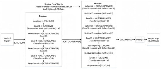
- Offset initialization: The offsets are initialized to 0; that is, Wdc and bdc are initially set to 0. During training, the offsets are learned progressively from small to large values. This process is consistent with the natural optimization trajectory, facilitates convergence to a favorable local optimum, and improves training stability. Figure 2 shows the improved ASTERIS model.Figure 2. Schematic diagram of the improved ASTERIS model.
3.5. Frequency Domain Loss Constraint
3.5.1. Complex-Domain Loss
Let the image size be H × W. The predicted image and the target image are transformed from the spatial domain to the frequency domain using a two-dimensional Fourier transform, F. In this representation, low-frequency components mainly describe smooth background variations, including interferences such as noise and stray light, whereas high-frequency components encode star spot edges and fine details. The amplitude spectrum characterizes the energy of each frequency component, whereas the phase spectrum encodes positional information. For star spot centroiding, the phase spectrum is particularly important because the phase determines the position of the star spot and PSF symmetry. A constraint imposed on the amplitude spectrum only, namely , can preserve high-frequency energy but cannot ensure phase consistency, potentially introducing positional shifts or shape distortion. Therefore, the complex-domain loss constrains amplitude and phase simultaneously as follows:
where (u,v) denotes the frequency domain coordinates. This loss penalizes amplitude and phase discrepancies simultaneously. Specifically, the squared modulus of the complex difference can be expanded as follows:
where denotes the phase difference.
3.5.2. High-Frequency Weighted Mask
The useful high-frequency energy of a star spot is mainly distributed near the boundary frequency of the PSF, whereas low-frequency components are largely associated with background variation and stray light interference. To ensure that the frequency constraint focuses on star spot morphology rather than smooth background components, the normalized frequency radius is defined as follows:
The radius r lies in [0, 0.707]. Given a threshold r0, the mask is set to:
The weighted frequency domain loss is defined as follows:
The mask assigns greater emphasis to the mid- and high-frequency components that contain star spot boundary and shape information. At the same time, the mask suppresses low-frequency background interference and reduces unnecessary computation. The experiments in this study indicate that r0 = 0.2 provides the best restoration of star spot details, and the threshold selection procedure is discussed below in Section 4.4.2.
Main algorithm procedure for Complex-Domain Frequency Loss:
- 2D Discrete Fourier Transform:predicted image , target image
- Compute the complex difference :
- Compute the modulus of the difference :
- Generate high-frequency weighting mask: compute the mask M according to r0
- Weighted average loss: compute Lfreq with and M
- Return the loss value for backpropagation.
3.5.3. Loss Balance Coefficient
The frequency domain loss Lfreq is calculated in a manner consistent with L1stack in ASTERIS [23], i.e., it computes the differences between the single-frame output and the target according to Equation (7). Because the spatial domain losses L1stack and L2mean are multiplied by coefficients on the order of 1 × 10⁶ in the baseline model, a balance coefficient, lambdafreq, is introduced for Lfreq. The total loss is expressed as follows:
A grid search over Lambdafreq ∈ {0, 100, 500, 1000, 2000, 3000} identifies 1000 as the optimal value, and the Lambdafreq selection procedure is discussed in detail in Section 4.4.3.
3.6. Network Training
The model was trained using the Adam optimizer with an initial learning rate of 1 × 10⁻⁴, which is annealed to 1 × 10⁻⁵ through a cosine schedule. The batch size is set to 3, and the network is trained for 20 epochs. The learning rate of the deformable convolution offsets is set to 1 × 10⁻⁵ to avoid unstable offset updates and reduce the risk of convergence to a noise-induced local optimum.
A single training sample consists of a randomly selected sequence of 16 consecutive noisy window frames from the simulation dataset (described in Section 4.1 below). Following the Noise2Noise strategy, the model takes the 8 even-numbered frames as input and uses the 8 odd-numbered frames as the corresponding target. The L1stack loss and the Lfreq loss are computed between the 8-frame prediction and the 8-frame target, while the L2mean loss is computed between the temporal mean of the 8-frame prediction and the temporal mean of the 8-frame target.
4. Experimental Validation
4.1. Dataset and Evaluation Metrics
Dataset construction method: Real window images obtained through ground calibration are used, and the window size is 48 × 48. The star spot energy and diffusion radius are randomly set. For each star spot, 4000 windows are calibrated, and the calibrated centroid is allowed to vary within 0.2 pixels around the window center, with coordinates (25,25). Setting all centroids at the window center simulates ideal registration and alignment of all frame window images, whereas centroid fluctuation within 0.2 pixels represents the alignment result under real conditions. Reference [37] provides on-orbit measurement data of star spot centroid jitter, with typical root-mean-square jitter ranging from 0.1 to 0.3 pixels. Detector readout noise and spatial random stray light, which are uncorrelated between frames and have an expected value of approximately zero, are then added to each window image through a simulation program to simulate real on-orbit operating conditions. The dataset does not include inter-frame gradually varying stray light interference with a nonzero mean caused by solar illumination conditions. The peak signal-to-noise ratio (PSNR) of images containing stray light and readout noise ranges from −6 to 15 dB, with an average of 8 dB. Among these images, 800 windows are randomly selected for testing, with every eight images forming one group for denoising and restoration, including multi-frame stacking. This setting yields 100 groups of test conditions, and the remaining images are used for training. The dataset comprises 30 star spots with distinct morphologies and brightness distributions. For each star spot, 4000 window images are generated under identical SNR parameter settings, thus yielding comparable average PSNR across all star spots. The images of each star spot are divided in a 4:1 ratio for training and testing respectively. The training images from all 30 spots are aggregated sequentially into a single training set of 96,000 images (30 × 3200) to enhance model generalization across varying star spot characteristics. The test data remain separated per star spot, forming 30 independent subsets, each consisting of 100 groups of 8-frame sequences (i.e., 30 × 100 test groups in total). This design enables evaluation of model performance on individual star spots and thus allows for a more detailed assessment of its generalization ability across diverse morphologies and brightness levels. The calculation formula for the peak signal-to-noise ratio is as follows:
where MAX denotes the maximum pixel value of the star spot, m × n denotes the image size, I denotes the original image before noise addition, and K denotes the noisy image to be evaluated.
Evaluation metrics: The evaluation metrics include the peak signal-to-noise ratio, the centroiding error standard deviation, and the noise standard deviation () [38]. The centroiding error standard deviation is defined as the standard deviation of the deviations between the centroid obtained from the denoised image and the window center and is expressed in pixels. The “Local window Centroiding Method” (the gray-scale center-of-gravity (CoG) method, where the star extraction threshold is defined as the background mean of the star-containing window plus 2.3 times its standard deviation. This factor is a sensitive parameter of the algorithm; in this study, its default value is adopted.) is used for centroid extraction, and the noise standard deviation is calculated as follows, where a smaller value indicates a smoother denoised image:
where N denotes the total number of pixels, I denotes the original image before noise addition, and J denotes the noisy image to be evaluated.
4.2. Experimental Results and Comparison with Multi-Frame Stacking (Mean), BM3D, and the Original ASTERIS Model
Each star spot in the test set is processed using multi-frame stacking, BM3D (all test images are normalized, and the prior coefficient sigma is set to 0.1), the ASTERIS model, and the proposed model (ours), namely deformable convolution combined with the frequency domain loss constraint. Table 1 summarizes the statistical results for the signal-to-noise ratio of the window images and the centroiding error standard deviation.
Table 1.
Denoising results for the signal-to-noise ratio of window images and the centroiding error of 30 star spots.
The experimental comparison shows that the proposed model achieves much better signal-to-noise ratio improvement and higher centroiding accuracy than the other three methods. This result verifies that the two proposed improvements further enhance the denoising capability of the baseline ASTERIS model, and the results also support the theoretical analysis in Section 3 regarding the advantages of the proposed deep learning method over multi-frame stacking. The noise standard deviation indicates that multi-frame stacking leaves more residual noise after denoising and produces poorer background smoothness. On the low-SNR star images in this study, BM3D achieves a PSNR improvement comparable to that of multi-frame stacking, with a modest enhancement in centroiding accuracy. Both traditional methods are significantly inferior to the proposed deep learning method in terms of restoration metrics such as PSNR and centroiding accuracy.
In terms of time and space performance, on the same workstation (CPU + GPU), the proposed model reduces the storage footprint of the original ASTERIS model from 161.6 MB to 117.2 MB. Meanwhile, the inference time for processing 100 groups of 8-frame test images is approximately 2.5 s for both models, showing comparable efficiency.
4.3. Ablation Study
Ablation experiments are conducted separately on the two proposed improvements, and the results are shown in Table 2. When both improvements are ablated, the processing results are the same as those of the ASTERIS model in Table 1.
Table 2.
Denoising results for 30 star spots when deformable convolution or frequency domain loss constraint is ablated.
Table 2 shows that ablating deformable convolution has a greater impact on the signal-to-noise ratio and noise standard deviation, which aligns with the theoretical analysis that deformable convolution can adaptively compensate for inter-frame subpixel centroid jitter, thereby improving cross-frame fusion accuracy and enhancing the denoising effect. By contrast, ablating the frequency domain loss constraint has a greater impact on centroiding accuracy. This result is also consistent with the analysis that this loss encourages the model to focus on high-frequency image information and is therefore conducive to restoring the PSF morphology of star spots.
Both improvements have individual limitations, but their combination compensates for each other’s weaknesses, substantially boosting the baseline’s denoising and restoration performance. Frequency domain loss alone enhances both star spot details and high-frequency noise; deformable convolution alone handles jitter but tends to smooth the spot without high-frequency protection. When combined, deformable convolution provides precise spatial localization, allowing for the frequency domain loss to enhance high frequencies only within the star spot region, thus avoiding noise amplification and artifacts. It also suppresses low-frequency background noise, achieving simultaneous gains in SNR and morphology. The core mechanism is that the frequency domain loss supplies high-frequency energy, while deformable convolution ensures spatial selectivity—neither is dispensable.
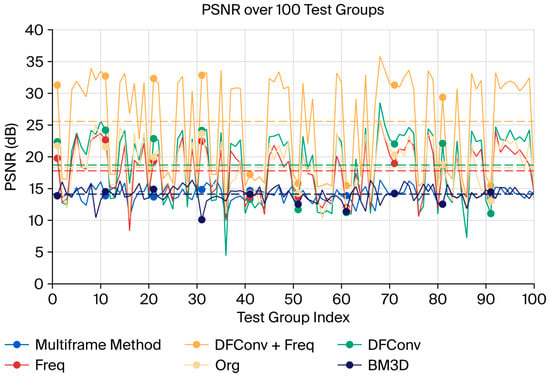
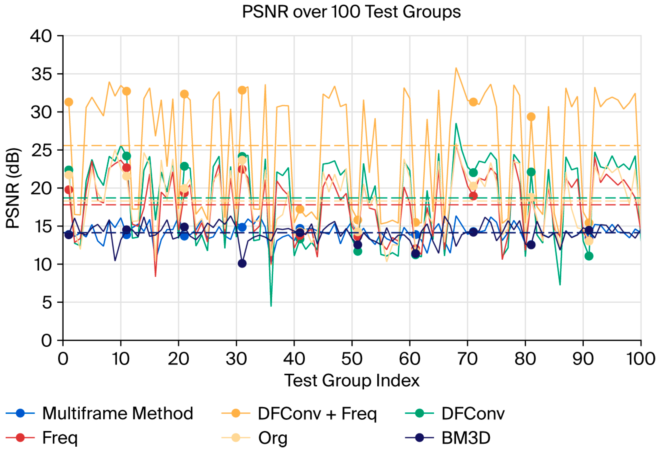
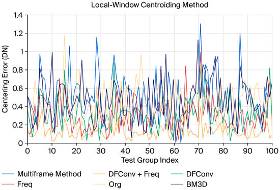
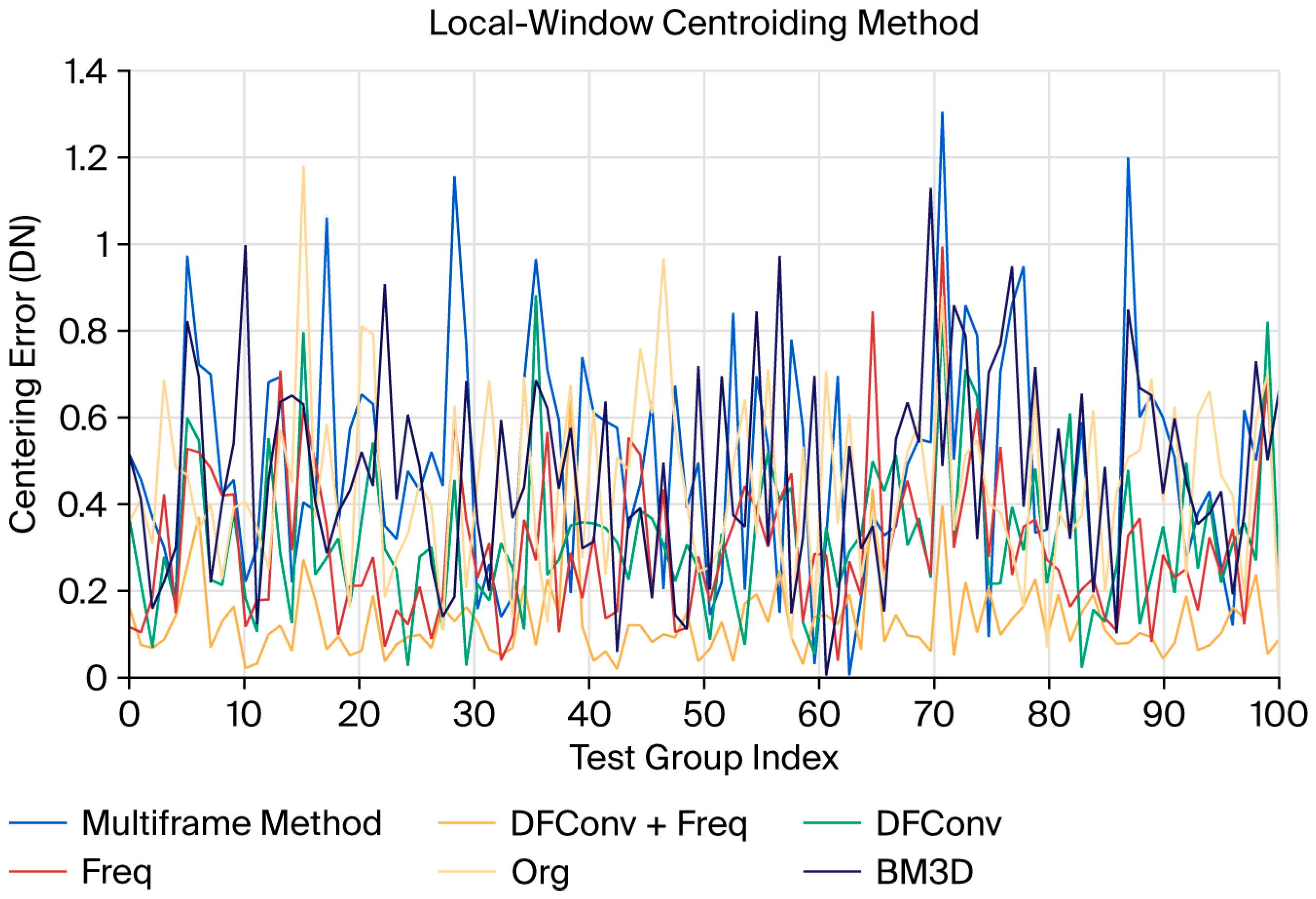
For one star spot in the test set with relatively weak energy, restoration is difficult; this subset contains 100 groups × eight noisy frames. Figure 3 and Figure 4 show the statistical curves of the window image-derived signal-to-noise ratio and centroiding error after processing using the six methods. In these figures, the curves labeled Multiframe Method, BM3D, DFConv + Freq, DFConv, Freq, and Org denote multi-frame stacking, BM3D, the proposed model, ASTERIS with only deformable convolution, ASTERIS with the frequency domain loss constraint only, and the ASTERIS model, respectively. The corresponding data are listed in Table 3.
Figure 3.
Statistical curve of the window image-derived PSNR for one star spot after processing using the six methods.
Figure 4.
Statistical curve of the window image-derived centroiding error for one star spot after processing using the six methods.
Table 3.
Denoising results for the window image-derived signal-to-noise ratio and the centroiding error of one star spot.
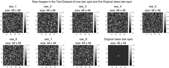
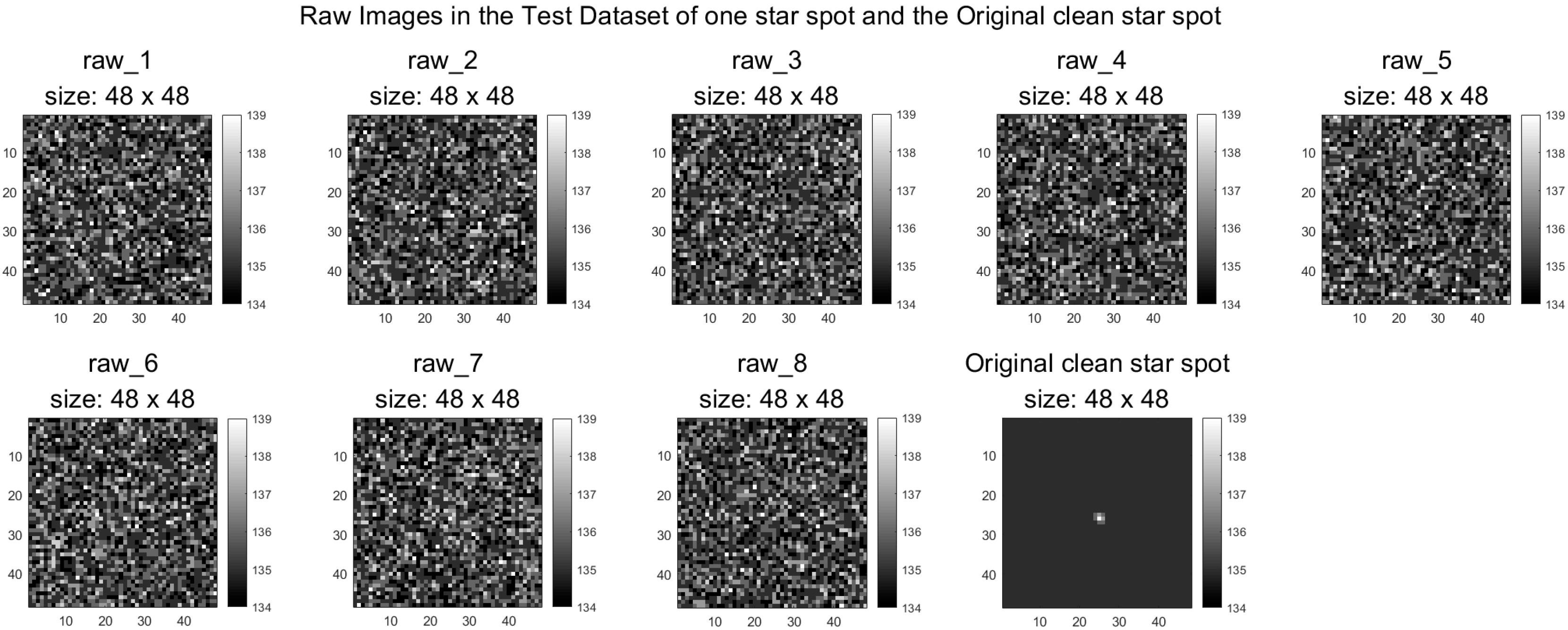
Figure 5 shows the original clean star spot and a group of eight noisy test images for this star spot, with an average PSNR of 8.18 dB. The star spot is almost submerged by noise, making centroid extraction impossible.
Figure 5.
A group of eight noisy images for one star spot.
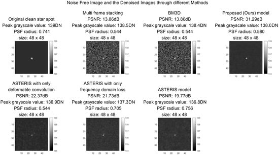
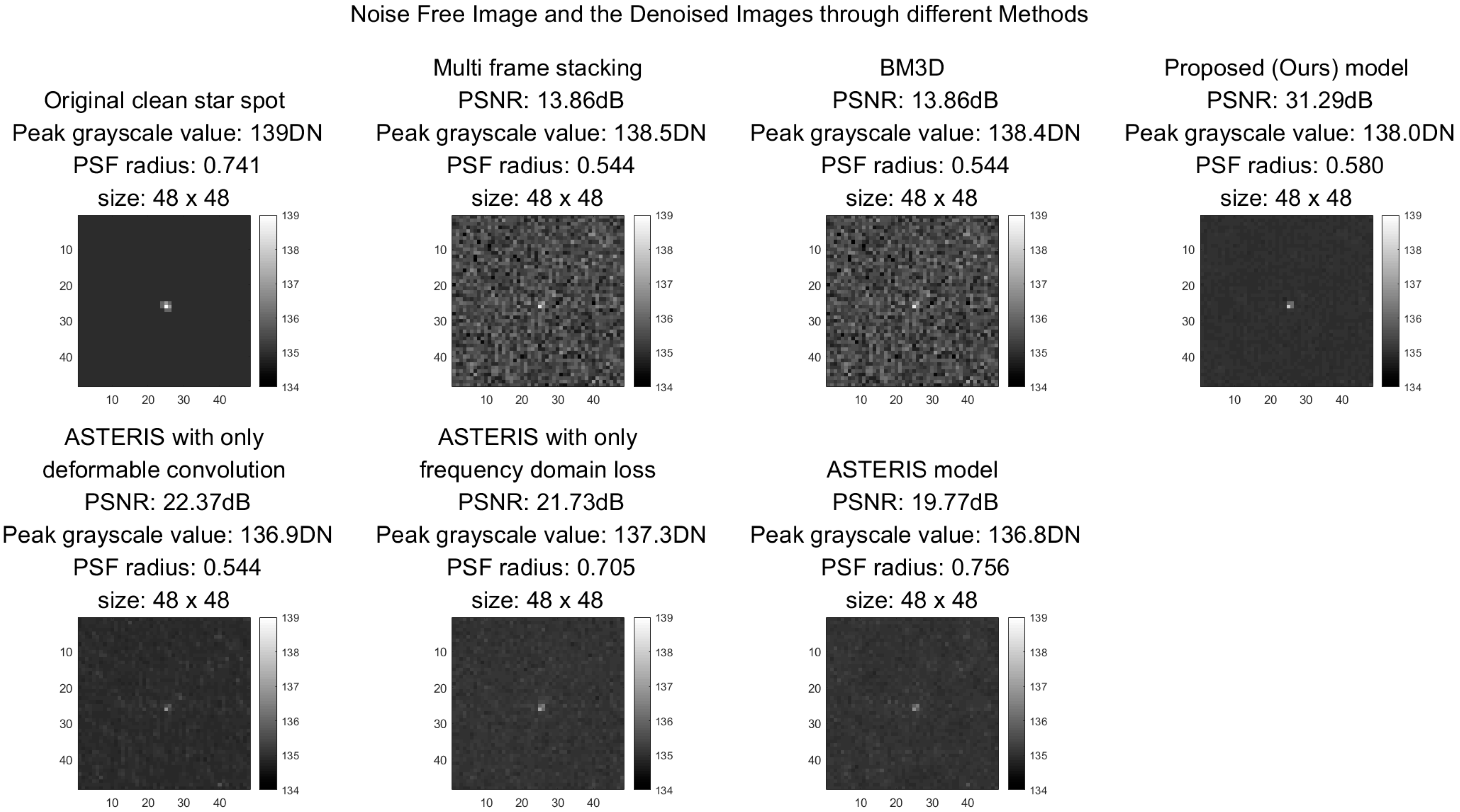
Figure 6 shows the denoised images obtained after processing the group of noisy images above using the six methods, together with the original noise-free star spot image.
Figure 6.
Comparison of the original noise-free image of one star spot and the results obtained by processing the group of noisy images above using six methods.
As shown in Figure 6, the proposed method achieves a substantially higher signal-to-noise ratio than the other methods after denoising, and the star spot is restored more accurately with clearer edges. By contrast, multi-frame stacking and BM3D yield a markedly lower signal-to-noise ratio and poorer background smoothness.
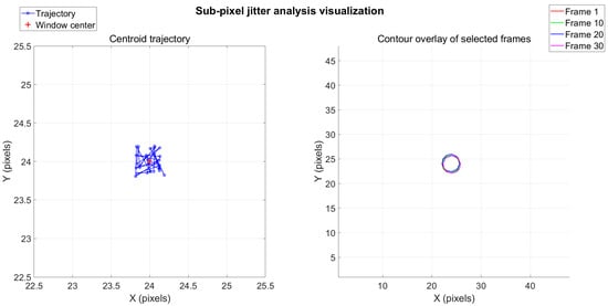
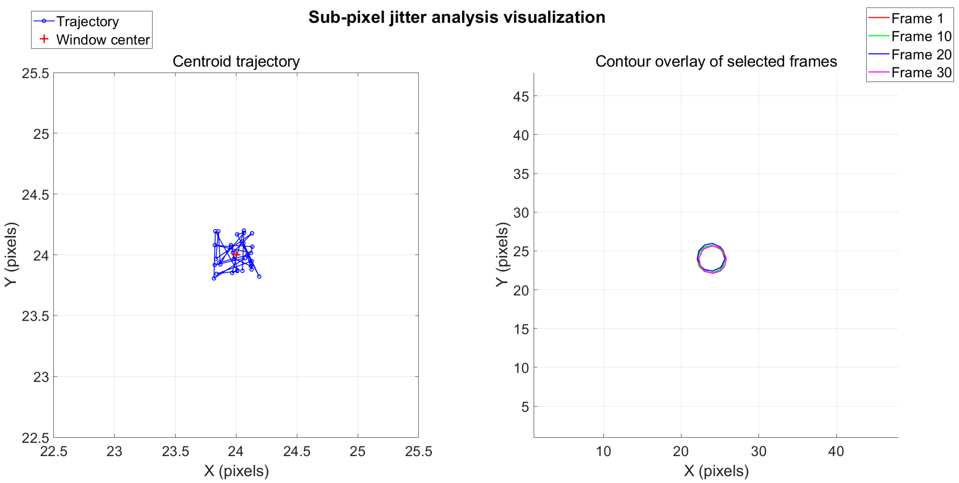
Figure 7 illustrates 30 frames, in each of which the star spot center is randomly shifted by ±0.2 pixels around the window center. The left subplot presents a zoomed-in view of the centroid trajectory, while the right subplot shows the contour overlays of selected frames, clearly revealing the subpixel jitter.
Figure 7.
Star spot center interframe subpixel jitter analysis visualization.
4.4. Parameter Tuning Study
4.4.1. Experiment with Deformable Convolution Placed in the Downsampling Stage
In this experiment, the deformable convolution module of the proposed model was moved from the decoder upsampling stage to the encoder downsampling stage to verify the theoretical analysis that deformable convolution is better suited for the upsampling stage, and the test results after identical training are shown in Table 4.
Table 4.
Experimental results with deformable convolution placed in the downsampling stage.
As shown above, placing deformable convolution in the downsampling stage yields results inferior to those obtained using the original ASTERIS model. In addition to the advantages of applying deformable convolution in the upsampling stage, as analyzed in Section 3.4.1, another important reason is that the inter-frame temporal dependencies are primarily captured by the encoder. Replacing the original standard 3D convolution with frame-by-frame 2D deformable convolution would result in the loss of temporal dependency information, thereby severely affecting the model’s ability to learn inter-frame noise and star spot variations.
4.4.2. Experiment on Tuning the High-Frequency Weighting Mask Threshold r0
The high-frequency weighting mask threshold r0 mentioned in Section 3.5.2 was grid-searched over r0 ∈ {0.0, 0.1, 0.2, 0.3}. This threshold influences the degree of attention paid to high-frequency components during training: a larger r0 focuses the model on higher frequencies while ignoring lower ones. The test results after identical training are shown in Table 5.
Table 5.
Experimental results of tuning r0.
When r0 is small, the sensitivity of the model to high-frequency components decreases, making low-frequency background suppression less effective, thus reducing both PSNR and centroiding accuracy. When r0 is too large, the model becomes overly sensitive to high frequencies, amplifying the influence of high-frequency noise, which also degrades PSNR and centroiding accuracy. Moreover, if such high-frequency noise occurs near a star spot, it may induce side lobes in the restored star spot, affecting centroiding results. The experiments show that r0 = 0.2 yields the best star image restoration performance.
4.4.3. Experiment on Tuning the Frequency Domain Loss Weight Coefficient Lambdafreq
The weight coefficient Lambdafreq of the frequency domain loss (Section 3.5.3) was grid-searched over Lambdafreq ∈ {0, 100, 500, 1000, 2000, 3000}, and a larger weight increases the influence of the frequency domain loss during training while reducing the influence of the spatial domain loss. The test results after identical training are shown in Table 6.
Table 6.
Experimental results of tuning lambdafreq.
As shown in the table, the best overall performance is achieved when Lambdafreq = 1000. Deviations from this value cause either under-preservation (when Lambdafreq is too small) or over-enhancement (when Lambdafreq is too large) of high-frequency components. The spatial domain loss enforces smooth pixel transitions; neglecting it leads to uneven backgrounds and star spot gray-level distributions inconsistent with the physical imaging model. Optimal training is achieved when the spatial domain loss and the frequency-domain loss are balanced in magnitude.
4.5. Generalization Study
4.5.1. Experiment on Inter-Frame Centroid Jitter-Free Condition
The training dataset used in this study contains inter-frame jitter within the range of [0, 0.2] pixels. Testing under the jitter-free condition serves as an evaluation of the model’s generalization capability and further validates the effectiveness of the two proposed improvements. A new set of test data was generated using the same star spot described in Section 4.3, with all 800 test window images having their star spot centroids fixed at the window center (i.e., no subpixel jitter introduced). The pre-trained models were then evaluated, and the test results for the original ASTERIS model, the proposed model, and the ASTERIS model with each of the two improvements individually are presented in Table 7 below.
Table 7.
Statistical results of window image SNR and centroiding error for deep learning methods under the jitter-free condition.
As shown in Table 7, under the jitter-free condition, the original ASTERIS model already achieves promising denoising performance, confirming its generalization capability. Neither the frequency domain loss nor deformable convolution alone brings significant improvement in SNR or centroiding accuracy. The frequency domain loss alone inherently suffers from the limitation described in Section 4.3 above: it tends to enhance both star spot details and high-frequency noise, yielding limited SNR gain when the baseline denoising is already strong, and in certain cases may introduce side-lobes that degrade centroiding accuracy. Deformable convolution alone primarily compensates for subpixel jitter; when centroids are already aligned, its SNR benefit is marginal, confirming its dedicated role. Moreover, for random noise without fixed spatial patterns, spatial offset sampling alone provides limited suppression. When combined, however, the two modules yield clear improvements in both SNR and centroiding accuracy. This confirms that deformable convolution provides precise spatial localization, enabling the frequency domain loss to enhance high frequencies only within the star spot region, thereby avoiding noise amplification and artifacts. This synergy leads to a dual enhancement in SNR and star spot morphology.
4.5.2. Experiment on Generalization to Unseen Star Morphologies
A new star spot was generated with distinct morphology characteristics (brightness, PSF radius, and grayscale distribution) that differ from those of the 30 star spots used for training. Following the dataset generation procedure described in Section 4.1 above, a test dataset of 800 window images was created for this new star spot. The pre-trained models were then evaluated, and the test results for the original ASTERIS model and the proposed model are presented in Table 8 below.
Table 8.
Test results on the new star spot dataset.
As shown in Table 8, the test results of both deep learning models are generally consistent with those reported in Table 3 of Section 4.3. This is because the ASTERIS model adopts a 3D spatiotemporal self-supervised learning strategy, which, in principle, is insensitive to star spot morphology characteristics such as brightness and PSF radius. Therefore, the original ASTERIS model itself already exhibits strong generalization capability across different star spot morphologies. Factors that significantly affect model training are primarily the noise intensity, noise mean level, and inter-frame jitter, rather than the morphological variations of the star spots.
5. Discussion and Future Work
This study proposes a deep learning method based on frame-by-frame spatial deformable convolution and complex-domain frequency domain constraints for star sensor window images degraded by detector readout noise, which follows a Gaussian distribution, and spatially random stray-light interference, which is independent between frames and has a mean of approximately zero. With ASTERIS as the baseline, the proposed method retains the advantages of the baseline model while introducing two improvements: frame-by-frame spatial deformable convolution in the decoder upsampling stage and a complex-domain frequency domain loss constraint. These improvements compensate for subpixel jitter of star spots, enhance denoising capability, preserve the high-frequency morphology of star spots, and reduce the number of model parameters by approximately one quarter. In the experiments, the proposed method achieves substantially better denoising performance than multi-frame stacking, BM3D and the baseline ASTERIS model. The proposed method improves PSNR by approximately 17.8 dB, and the centroiding error reaches approximately 0.1 pixels, which is smaller than the artificially added centroid jitter range in the test set, which was approximately 0.2 pixels.
For interference with a nonzero mean, any method that relies on temporal independence only, including multi-frame stacking and self-supervised learning, cannot remove the mean component. Although the proposed method theoretically cannot eliminate this component, its spatially adaptive filtering capability enables better suppression of background spatial nonuniformity than multi-frame stacking and can reduce star spot centroiding errors.
Future work will introduce a background estimation branch into the model, allowing for the static background to be subtracted at the input end through a learnable background separation network. This extension is expected to improve the adaptability of the proposed method to complex on-orbit environments and diverse remote sensing tasks. Lightweight network design and dynamically adaptive frequency domain loss weighting are also important directions for future research. Real on-orbit star image data will be acquired from various on-orbit missions to construct more diverse test benchmarks to verify and improve the generalization capability against unknown noise distributions and stray light patterns of the model, thereby laying a solid foundation for eventual engineering deployment.
Author Contributions
J.G.: conceptualization, methodology, validation, visualization, investigation, and writing—original draft, review, and editing. H.Y.: data curation, resources, methodology, investigation, and writing—original draft, review, and editing. Y.W.: conceptualization, resources, investigation, review, and editing. X.L.: conceptualization, review, and editing. R.C.: data curation, resources, investigation, review, and editing. All authors have read and agreed to the published version of the manuscript.
Funding
This research was funded by the China Civil Aerospace Space Debris Special Project (Grant No. D020101).
Data Availability Statement
The simulated windowed image datasets generated and analyzed in this study have not been publicly archived at present but are available from the corresponding author upon reasonable request. The source code is available from the corresponding author (Y.W., 20033110168@stu.xidian.edu.cn) to support result reproduction or research extension. All underlying data required to understand, evaluate, and build upon the reported findings are provided in this article.
Acknowledgments
The authors gratefully acknowledge Xiaogang Dong, Cong Tian, and Miaomiao Wang for their valuable guidance and suggestions throughout this research.
Conflicts of Interest
The authors declare no conflict of interest.
References
- Liebe, C. Star trackers for attitude determination. IEEE Aerosp. Electron. Syst. Mag. 1995, 10, 10–16. [Google Scholar] [CrossRef] [Scilit]
- Eisenman, A.R.; Liebe, C.C.; Joergensen, J.L. New generation of autonomous star trackers. In Proceedings of the SPIE‘s 1997 International Symposium on Optical Science, Engineering and Instrumentation, San Diego, CA, USA, 27 July–1 August 1997; Volume 3219, pp. 210–224. [Google Scholar] [CrossRef] [Scilit]
- Wang, H.; Jiang, J.; Zhang, G. A high-precision star tracker for spacecraft attitude determination. IEEE Trans. Aerosp. Electron. Syst. 2019, 55, 2475–2485. [Google Scholar] [CrossRef]
- Mehta, D.S.; Parsa, K. A star pattern recognition technique for star trackers. Adv. Space Res. 2019, 64, 2055–2068. [Google Scholar] [CrossRef] [Scilit]
- Rufino, G.; Accardo, D. Enhancement of the centroiding algorithm for star tracker measure refinement. Acta Astronaut. 2003, 53, 135–147. [Google Scholar] [CrossRef] [Scilit]
- Marcelino, G.M.; Schulz, V.H.; Seman, L.O.; Bezerra, E.A. Centroid determination hardware algorithm for star trackers. Int. J. Sens. Netw. 2020, 32, 1–14. [Google Scholar] [CrossRef] [Scilit]
- Hou, Y.; Zhao, R.; Ma, Y.; He, L.; Zhu, Z. An on-orbit correction method for high dynamic APS star tracker based on adaptive filtering. Acta Photonica Sin. 2021, 50, 155. [Google Scholar] [CrossRef] [Scilit]
- Tomasi, C.; Manduchi, R. Bilateral filtering for gray and color images. In Proceedings of the IEEE International Conference on Computer Vision, Bombay, India, 7 January 1998; pp. 839–846. [Google Scholar] [CrossRef] [Scilit]
- Donoho, D. De-noising by soft-thresholding. IEEE Trans. Inf. Theory 1995, 41, 613–627. [Google Scholar] [CrossRef] [Scilit]
- Portilla, J.; Strela, V.; Wainwright, M.; Simoncelli, E. Image denoising using scale mixtures of Gaussians in the wavelet domain. IEEE Trans. Image Process. 2003, 12, 1338–1351. [Google Scholar] [CrossRef] [Scilit] [PubMed]
- Buades, A.; Coll, B.; Morel, J.M. A review of image denoising algorithms, with a new one. Multiscale Model. Simul. 2005, 4, 490–530. [Google Scholar] [CrossRef] [Scilit]
- Lebrun, M.; Buades, A.; Morel, J.M. A nonlocal Bayesian image denoising algorithm. SIAM J. Imaging Sci. 2013, 6, 1665–1688. [Google Scholar] [CrossRef] [Scilit]
- Gu, S.; Zhang, L.; Zuo, W.; Feng, X. Weighted nuclear norm minimization with application to image denoising. In Proceedings of the IEEE Conference on Computer Vision and Pattern Recognition, Columbus, OH, USA, 24–27 June 2014; pp. 2862–2869. [Google Scholar] [CrossRef] [Scilit]
- Dabov, K.; Foi, A.; Katkovnik, V.; Egiazarian, K. Image denoising by sparse 3-D transform-domain collaborative filtering. IEEE Trans. Image Process. 2007, 16, 2080–2095. [Google Scholar] [CrossRef] [Scilit] [PubMed]
- Maggioni, M.; Katkovnik, V.; Egiazarian, K.; Foi, A. Nonlocal transform-domain filter for volumetric data denoising and reconstruction. IEEE Trans. Image Process. 2013, 22, 119–133. [Google Scholar] [CrossRef] [Scilit] [PubMed]
- Savarese, S.; Rabinovich, A.; Stergiopoulos, S. Multi-frame alignment and denoising for faint star detection in star trackers. In Proceedings of the AIAA Guidance, Navigation, and Control Conference; AIAA: Reston, VA, USA, 2020; pp. 1234–1245. [Google Scholar] [CrossRef] [Scilit]
- Li, B.; Ye, Z.; Zhang, X.; Zheng, X.; Sun, J. An autocorrelation-based multi-frame adding method for faint star extraction. Infrared Laser Eng. 2025, 54, 20250184. [Google Scholar] [CrossRef] [Scilit]
- Wang, X.; Wang, X. Multiple targets sparse matching for binocular vision positioning system with large field of view. Infrared Laser Eng. 2018, 47, 0726001. [Google Scholar] [CrossRef] [Scilit]
- Zhao, H.; Lembeck, M.F.; Zhuang, A.; Shah, R.; Wei, J. Real-time convolutional-neural-network-based star detection and centroiding method for CubeSat star tracker. IEEE Trans. Aerosp. Electron. Syst. 2025, 61, 8172–8184. [Google Scholar] [CrossRef] [Scilit]
- Ronneberger, O.; Fischer, P.; Brox, T. U-Net: Convolutional networks for biomedical image segmentation. In Proceedings of the International Conference on Medical Image Computing and Computer-Assisted Intervention, Munich, Germany, 5–9 October 2015; pp. 234–241. [Google Scholar] [CrossRef] [Scilit]
- Içek, Ö.; Abdulkadir, A.; Lienkamp, S.S.; Brox, T.; Ronneberger, O. 3D U-Net: Learning dense volumetric segmentation from sparse annotation. In Proceedings of the International Conference on Medical Image Computing and Computer-Assisted Intervention, Athens, Greece, 17–21 October 2016; pp. 424–432. [Google Scholar] [CrossRef] [Scilit]
- Zamir, S.W.; Arora, A.; Khan, S.; Hayat, M.; Khan, F.S.; Yang, M. Restormer: Efficient transformer for high-resolution image restoration. In Proceedings of the IEEE/CVF Conference on Computer Vision and Pattern Recognition, New Orleans, LA, USA, 18–24 June 2022; pp. 5728–5739. [Google Scholar] [CrossRef] [Scilit]
- Guo, Y.; Zhang, H.; Li, M.; Yu, F.; Wu, Y.; Hao, Y.; Huang, S.; Liang, Y.; Lin, X.; Li, X.; et al. Deeper detection limits in astronomical imaging using self-supervised spatiotemporal denoising. Science 2026, 392, ady9404. [Google Scholar] [CrossRef] [Scilit] [PubMed]
- Fang, B.-L.; Wang, J.-G.; Feng, G.-B. Calculation of spot centroid based on physical informed neural networks. Acta Phys. Sin. 2022, 71, 200601. [Google Scholar] [CrossRef] [Scilit]
- Dai, J.; Qi, H.; Xiong, Y.; Li, Y.; Zhang, G.; Hu, H.; Wei, Y. Deformable convolutional networks. In Proceedings of the IEEE International Conference on Computer Vision, Venice, Italy, 22 October 2017; pp. 764–773. [Google Scholar] [CrossRef] [Scilit]
- Peng, Y.; Xie, W.; Li, J.; Wu, S.; Wang, Z.; Hu, B.; Yao, J. LDG: Lightweight Deformable 3D Gaussians for Single-View Dynamic Scene Reconstruction. In Proceedings of the 2025 IEEE International Conference on Acoustics, Speech and Signal Processing (ICASSP), Hyderabad, India, 6–11 April 2025; pp. 1–5. [Google Scholar] [CrossRef] [Scilit]
- Wang, Z.; Bovik, A.C.; Sheikh, H.R.; Simoncelli, E.P. Image quality assessment: From error visibility to structural similarity. IEEE Trans. Image Process. 2004, 13, 600–612. [Google Scholar] [CrossRef] [Scilit] [PubMed]
- Ćelić, J.; Lang, R.G.; Steinmassl, S.; Hinton, J.; Funk, S. A novel approach to optimizing the image cleaning performance of Imaging Atmospheric Cherenkov Telescopes. Astron. Astrophys. 2025, 699, A96. [Google Scholar] [CrossRef] [Scilit]
- Gong, X.; Li, T.; Wang, R.; Hu, S.; Yuan, S. Beyond the Remote Sensing Ecological Index: A Comprehensive Ecological Quality Evaluation Using a Deep-Learning-Based Remote Sensing Ecological Index. Remote Sens. 2026, 17, 558. [Google Scholar] [CrossRef] [Scilit]
- Zhu, C.; Deng, S.; Song, X.; Li, Y.; Wang, Q. Mamba Collaborative Implicit Neural Representation for Hyperspectral and Multispectral Remote Sensing Image Fusion. IEEE Trans. Geosci. Remote Sens. 2025, 63, 5504915. [Google Scholar] [CrossRef] [Scilit]
- Shah, Z.H.; Müller, M.; Hübner, W.; Ortkrass, H.; Hammer, B.; Huser, T.; Schenck, W. Image restoration in frequency space using complex-valued CNNs. Front. Artif. Intell. 2024, 7, 1353873. [Google Scholar] [CrossRef] [Scilit] [PubMed]
- Lehtinen, J.; Munkberg, J.; Hasselgren, J.; Laine, S.; Karras, T.; Aittala, M.; Aila, T. Noise2Noise: Learning image restoration without clean data. In Proceedings of the International Conference on Machine Learning, Stockholm, Sweden, 10–15 July 2018; pp. 2965–2974. [Google Scholar]
- Krull, A.; Buchholz, T.-O.; Jug, F. Noise2Void: Learning denoising from single noisy images. In Proceedings of the IEEE/CVF Conference on Computer Vision and Pattern Recognition, Long Beach, CA, USA, 16–20 June 2019; pp. 2129–2137. [Google Scholar] [CrossRef] [Scilit]
- Batson, J.; Royer, L. Noise2Self: Blind denoising by self-supervision. In Proceedings of the International Conference on Machine Learning, Long Beach, CA, USA, 9–15 June 2019; pp. 524–533. [Google Scholar] [CrossRef]
- Zhang, K.; Zuo, W.; Chen, Y.; Meng, D.; Zhang, L. Beyond a Gaussian denoiser: Residual learning of deep CNN for image denoising. IEEE Trans. Image Process. 2017, 26, 3142–3155. [Google Scholar] [CrossRef] [Scilit] [PubMed]
- Zhang, K.; Zuo, W.; Zhang, L. FFDNet: Toward a fast and flexible solution for CNN-based image denoising. IEEE Trans. Image Process. 2018, 27, 4608–4622. [Google Scholar] [CrossRef] [Scilit] [PubMed]
- Zhang, J. On the starspot centroid estimation and calibration technologies for the super-high accuracy star tracker. Aerospace 2024, 11, 448. [Google Scholar] [CrossRef] [Scilit]
- Liu, J.G.; Li, J.; Hao, Z.H. Study on detection sensitivity of APS star tracker. Opt. Precis. Eng. 2006, 14, 553–557. [Google Scholar] [CrossRef]

Disclaimer/Publisher’s Note: The statements, opinions and data contained in all publications are solely those of the individual author(s) and contributor(s) and not of MDPI and/or the editor(s). MDPI and/or the editor(s) disclaim responsibility for any injury to people or property resulting from any ideas, methods, instructions or products referred to in the content. |
© 2026 by the authors. Licensee MDPI, Basel, Switzerland. This article is an open access article distributed under the terms and conditions of the Creative Commons Attribution (CC BY) license.