Article

A Vertically Structured Machine Learning Approach for Cloud Liquid and Ice Water Content Profiling

1
School of Automation, Nanjing University of Information Science and Technology, Nanjing 210044, China
2
Department of Computer Science, University of Reading, Reading RG6 6DH, UK
3
China Meteorological Administration Aerosol-Cloud and Precipitation Key Laboratory, School of Atmospheric Physics, Nanjing University of Information Science and Technology, Nanjing 210044, China
4
State Key Laboratory of Severe Weather Meteorological Science and Technology, Chinese Academy of Meteorological Sciences, Beijing 100081, China
5
Guangxi Zhuang Autonomous Region Meteorological Observatory, Guangxi Zhuang Autonomous Region Meteorological Bureau, Nanning 530022, China
6
Open Laboratory of Guangxi Beibu Gulf National Climate Observatory, Guangxi Zhuang Autonomous Region Meteorological Bureau, Nanning 530022, China
7
Guangxi Zhuang Autonomous Region Meteorological Technology and Equipment Center, Nanning 530022, China
*
Author to whom correspondence should be addressed.
Remote Sens. 2026, 18(13), 2177; https://doi.org/10.3390/rs18132177
Submission received: 15 May 2026 / Revised: 25 June 2026 / Accepted: 29 June 2026 / Published: 3 July 2026
(This article belongs to the Special Issue Advanced AI Technology for Remote Sensing Analysis (Second Edition))

Highlights

What are the main findings?
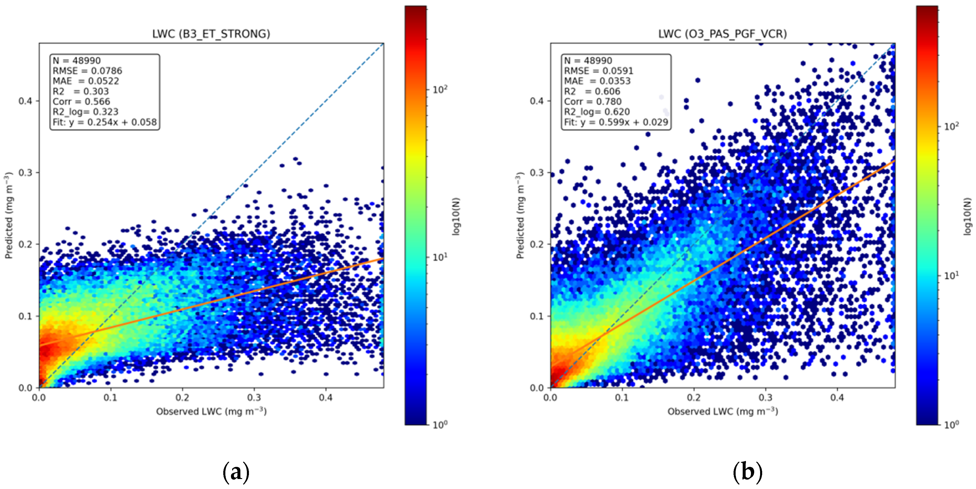
  • A vertically structured machine-learning framework improves cloud water retrieval accuracy, reducing RMSE from 0.0152 g m−3 to 0.0092 g m−3 for IWC and from 0.0786 g m−3 to 0.0591 g m−3 for LWC.
  • Explicit modelling of vertical dependencies produces more vertically coherent cloud profiles compared with conventional pointwise approaches.
What are the implications of the main findings?
  • Incorporating vertical structure is critical for improving data-driven retrieval of atmospheric profiles, particularly in mixed-phase cloud conditions.
  • The proposed framework provides a scalable strategy for multisource cloud retrieval and has potential applications in atmospheric remote sensing and data assimilation.

Abstract

Accurate retrieval of cloud liquid water content (LWC) and ice water content (IWC) vertical profiles remains limited by strong vertical variability and nonlinear dependencies among observed variables. Ground-based cloud radar reflectivity and microwave radiometer-derived thermodynamic profiles provide complementary constraints, but their joint use requires consistent time–height matching and bias-controlled predictors. This study develops a vertically structured machine-learning framework that explicitly represents profile-level dependencies by constructing vertical-structure-enhanced features to encode local gradients and contextual information, integrating multiple tree-based learners with heterogeneous configurations through a profile-aware stacking strategy, and introducing a profile-level refinement step to suppress layer-to-layer inconsistencies. The framework is evaluated using year-round Cloudnet observations from the Lindenberg site, where IWC RMSE decreases from 0.0152 g m−3 to 0.0092 g m−3 with R2 increasing from 0.412 to 0.784, and LWC RMSE decreases from 0.0786 g m−3 to 0.0591 g m−3 with R2 increasing from 0.303 to 0.606. Additional boundary-region evaluation shows that the improvement is particularly evident near radar-derived cloud boundaries, where cloud structure and hydrometeor content may vary rapidly with height. These results indicate that treating cloud retrieval as a vertically structured learning problem reduces inconsistencies inherent in pointwise models and establishes a data-driven baseline for incorporating vertical constraints into atmospheric profile retrieval.

1. Introduction

Clouds and precipitation systems are central components of the atmospheric energy and water cycles, and their representation remains a major source of uncertainty in weather and climate prediction [1]. Among cloud microphysical variables, liquid water content (LWC) and ice water content (IWC) are particularly important because they describe not only the amount of condensed water, but also its phase and vertical distribution. These vertical profiles are closely linked to cloud radiative effects, precipitation development, and cloud lifetime [2]. Because liquid droplets and ice particles interact differently with shortwave and longwave radiation, uncertainty in their vertical partitioning can affect estimates of cloud radiative effects and the atmospheric energy balance [3]. In mixed-phase clouds, the relative amount and spatial distribution of liquid water and ice further influence cloud lifetime, precipitation processes, climate feedbacks, and radiative properties [4,5,6]. Reliable profiling of LWC and IWC is therefore essential for understanding cloud processes and evaluating their representation in models.
Mixed-phase clouds are especially difficult to observe and model. They contain supercooled liquid droplets, ice particles, and water vapour under subfreezing conditions, and their evolution involves ice nucleation, vapour deposition, aggregation, riming, and other coupled microphysical pathways [7]. Their phase partitioning is also shaped by thermodynamic conditions, aerosol abundance, and dynamical processes, which can modulate ice formation in stratiform cloud layers [8]. These uncertainties have broader climate implications. A realistic representation of the supercooled liquid fraction has been linked to constraints on equilibrium climate sensitivity [9], and recent observational constraints on supercooled cloud feedbacks have been shown to reduce uncertainty in projected warming [10]. When mixed-phase processes are not well represented, models can develop biases in cloud state and thermodynamic structure, including Arctic wintertime temperature inversions [11]. These issues highlight the need for observational methods that can resolve both liquid and ice water profiles in the vertical.
Accurate LWC and IWC profiles are commonly retrieved by combining observations that describe cloud vertical structure with information on the surrounding thermodynamic environment. Cloud radar, lidar, and microwave radiometer measurements provide complementary information for this task. Cloud radar reflectivity is sensitive to particle size and can penetrate optically thicker cloud layers, while lidar is sensitive to small droplets, aerosols, and cloud boundaries [12]. Cloud phase information is often a prerequisite for retrieving cloud properties, because phase uncertainty can propagate into LWC and particle-size retrievals [13]. Ground-based multisensor phase classification has therefore become an important basis for cloud-property retrieval [14]. Cloudnet provides a broader framework by integrating radar, lidar, microwave radiometer, and model data into continuous time–height products of cloud classification and hydrometeor properties [15]. Cloud-property retrievals in the Atmospheric Radiation Measurement (ARM) programme have also demonstrated the value of combining active remote sensing, microwave radiometer, and thermodynamic information for cloud microphysical studies [16,17]. The Cloudnet processing chain has since been implemented in CloudnetPy, supporting standardized processing of cloud remote-sensing datasets [18]. Recent Cloudnet-based campaign products further show that such frameworks can provide LWC, IWC, cloud classification, and cloud macro- and microphysical properties at high temporal and vertical resolution [19].
Despite this observational foundation, converting multisensor measurements into reliable LWC and IWC profiles remains challenging. Physically based synergistic retrievals, such as variational radar–lidar–radiometer methods, have provided an important framework for retrieving ice-cloud properties from combined observations [20]. More recent EarthCARE retrieval developments extend this idea toward unified active–passive retrievals of clouds, aerosols, and precipitation [21]. However, mixed-phase retrieval remains more difficult than single-phase retrieval because liquid, ice, and mixed-phase regions produce different observational responses and cannot always be processed using one set of assumptions [12]. Lidar–radar synergistic retrievals are also limited when lidar signals become fully attenuated, preventing full-column characterization of cloud liquid in optically thick or multilayer mixed-phase clouds [22,23]. Cloud radar Doppler spectra can provide information beyond the lidar attenuation height, but liquid and ice signatures may be difficult to separate when turbulence broadens the spectra or when the liquid signal is weak [24,25]. Rapid changes in phase partitioning near mixed-phase transition regions add further vertical and temporal variability [26]. Updates to DARDAR-CLOUD, a combined radar–lidar cloud classification and ice-cloud property product, also show that retrieved microphysical properties can be sensitive to parameter choices and assumed particle relationships [27]. These limitations suggest that cloud-water retrieval depends not only on instrument availability, but also on how multisensor information is collocated, corrected, and represented vertically.
Machine-learning methods offer a complementary way to extract liquid- and phase-related information from complex remote-sensing observations. Interest in machine learning and deep learning has increased rapidly in Earth system science, partly because these methods can learn nonlinear relationships from large observational datasets [28]. In cloud-radar applications, artificial neural networks have been used to infer riming from Doppler radar variables such as reflectivity, spectrum width, and skewness [29]. Supervised learning has also been used for radar Doppler spectra peak finding, and structure-preserving spectral analysis methods have been developed to describe the morphology of Doppler spectra [30,31]. More directly related to liquid detection, deep convolutional neural networks have been used to infer the probability of supercooled cloud droplets from vertically pointing Doppler cloud radar observations, using Cloudnet target classification as supervision [32]. Related work has evaluated Artificial Neural Network-based liquid classification against Cloudnet target classification and independent measurements such as microwave-radiometer liquid water path, ceilometer cloud-base height, radiosonde humidity, and satellite lidar observations [22]. Recent multisensor machine-learning studies have also shown that random forests, multilayer perceptrons, and convolutional neural networks can use radar, lidar, microwave radiometer, and radiosonde inputs for thermodynamic cloud-phase classification [33]. Earlier neural-network applications in atmospheric remote sensing include retrievals of precipitable water vapour and liquid water path from ground-based radiometer observations, cirrus cloud retrieval from satellite thermal observations, and analysis of marine liquid-water cloud occurrence from global observations [34,35,36].
These studies show that data-driven methods can extract useful information from radar spectra, multisensor cloud observations, and reference products such as Cloudnet. However, most existing machine-learning applications in this area focus on phase classification, liquid-layer detection, cloud occurrence, or column-integrated quantities. They do not directly address the joint retrieval of vertically coherent LWC and IWC profiles. This distinction is important because cloud water content is not simply a collection of independent point values. LWC and IWC evolve with height through thermodynamic stratification, hydrometeor growth, cloud-boundary transitions, and phase changes. A pointwise regression framework may therefore lose part of the vertical coherence required for physically consistent retrieval, especially near cloud boundaries and mixed-phase transition regions.
This study addresses this gap by reformulating LWC and IWC retrieval as a vertically structured learning problem. Instead of treating each height level as an isolated sample, the proposed approach treats the cloud profile as the basic unit of representation. Year-round Cloudnet observations from the Lindenberg site in 2025 are used as the primary dataset, with Cloudnet-derived LWC and IWC profiles serving as reference targets. Reflectivity from the METEK MIRA-35 Ka-band Doppler cloud radar (METEK Meteorologische Messtechnik GmbH, Elmshorn, Germany), a 35 GHz cloud radar system, was used as the main vertically resolved observational predictor, while microwave-radiometer-derived temperature and relative humidity profiles describe the thermodynamic environment. Radiosonde observations are first used to evaluate and reduce height-dependent thermodynamic biases, improving the consistency of the predictor space before model training. The proposed framework then combines vertical-structure-enhanced features, profile-aware stacking of tree-based learners, and profile-level refinement based on cloud-geometry information. Through this design, the study evaluates whether explicit representation of vertical structure can improve both pointwise accuracy and profile-level coherence in data-driven LWC and IWC retrieval from collocated ground-based radar and thermodynamic observations.

2. Materials and Methods

2.1. Method and Processing Workflow

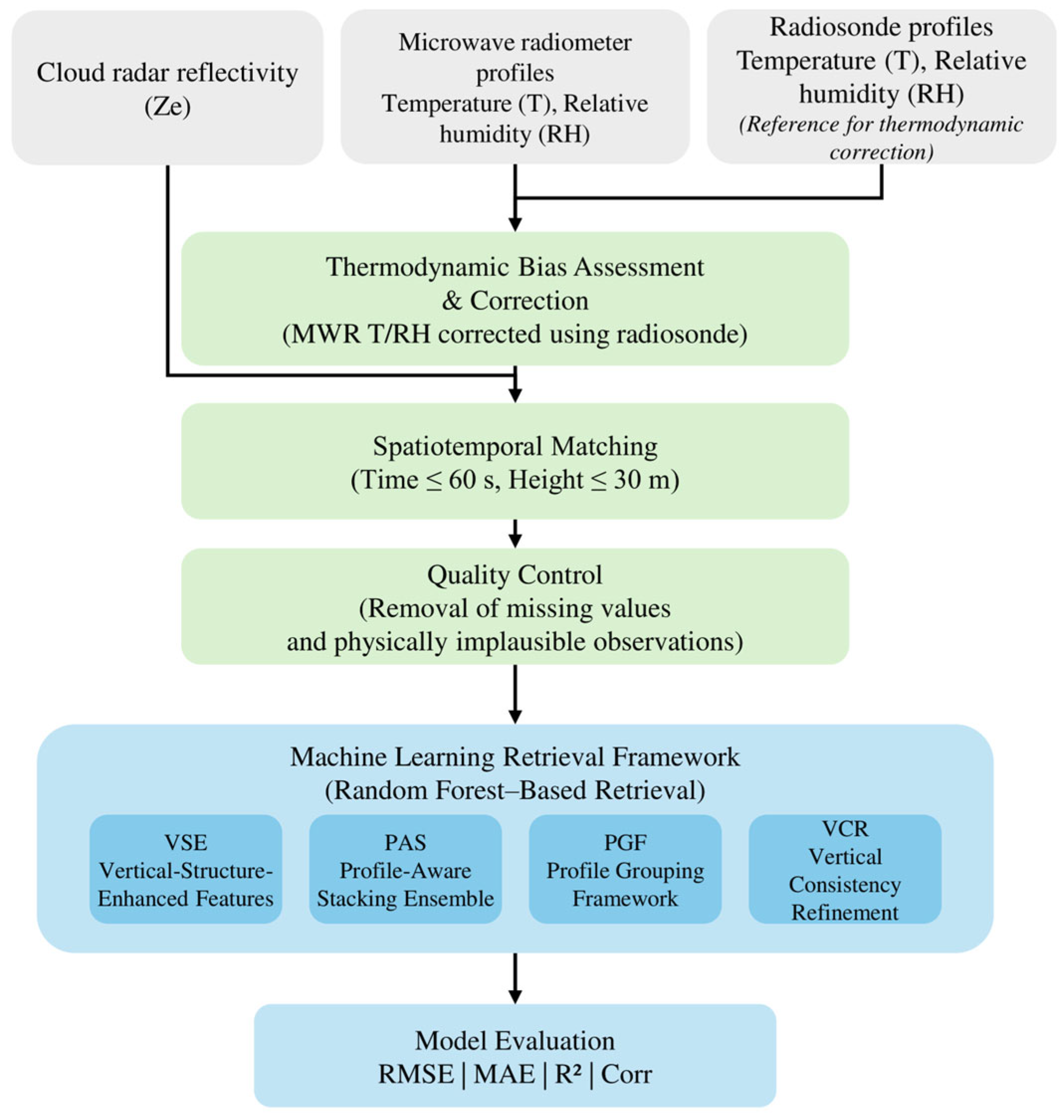
The overall methodological workflow is shown in Figure 1. This study combines Cloudnet hydrometeor products, METEK MIRA-35 cloud radar reflectivity (METEK Meteorologische Messtechnik GmbH, Elmshorn, Germany), HATPRO-G5 microwave-radiometer-derived temperature and relative humidity profiles (Radiometer Physics GmbH, Meckenheim, Germany), and radiosonde observations. The microwave-radiometer-derived thermodynamic profiles are first assessed and corrected using radiosonde measurements as an independent reference. The corrected thermodynamic profiles are then matched with cloud radar reflectivity and Cloudnet hydrometeor products in time and height, followed by quality control. The resulting collocated dataset is used to train a vertically structured machine-learning framework for retrieving liquid water content (LWC) and ice water content (IWC) profiles. The following subsections describe the observational datasets, thermodynamic consistency correction, retrieval dataset construction, model design, and evaluation strategy.

2.2. Study Site and Observational Datasets

2.2.1. Study Site and Observation Period

Year-round observations from the Cloudnet Lindenberg site in Germany in 2025 were used as the primary dataset for this study. The Lindenberg dataset was used for model development, model training, internal testing, and the main evaluation of liquid water content (LWC) and ice water content (IWC) profile retrieval.
Additional observations from the Munich and Jülich Cloudnet sites were used to assess cross-site transferability, as described in Section 2.2.5 and Section 2.6.5.

2.2.2. Cloudnet LWC/IWC Target Products

Cloudnet is a ground-based cloud remote-sensing processing framework that combines active and passive observations with auxiliary atmospheric information to provide vertically resolved cloud classification and hydrometeor products. At Cloudnet sites, measurements from instruments such as cloud radar, lidar or ceilometer, and microwave radiometer are processed together with atmospheric model information to generate time–height cloud products suitable for cloud-process studies and model evaluation.
In this study, the Lindenberg Cloudnet products for 2025 were used as the primary reference dataset. The Cloudnet-derived liquid water content (LWC) and ice water content (IWC) profiles were used as supervised learning targets for the retrieval models. The associated observational predictors included METEK MIRA-35 Ka-band radar reflectivity (METEK Meteorologische Messtechnik GmbH, Elmshorn, Germany) and HATPRO-G5 microwave-radiometer-derived thermodynamic profiles of temperature and relative humidity (Radiometer Physics GmbH, Meckenheim, Germany). These variables were selected because they provide complementary information on cloud vertical structure and the surrounding thermodynamic environment.
The Cloudnet LWC and IWC products were treated as reference retrieval products rather than direct in situ measurements. They provide a physically consistent and vertically resolved benchmark for model development, but they may contain uncertainties related to instrument sensitivity, retrieval assumptions, cloud phase, and microphysical parameterisations. These uncertainties are particularly relevant in mixed-phase clouds, where liquid and ice hydrometeors may coexist within the same atmospheric column. Nevertheless, Cloudnet products offer a practical and internally consistent reference for developing data-driven LWC and IWC retrieval models from ground-based remote-sensing observations.

2.2.3. Radar Reflectivity and Thermodynamic Predictors

Two types of observational predictors were used in this study: cloud radar reflectivity and thermodynamic profiles. Cloud radar reflectivity was obtained from the METEK MIRA-35 Ka-band cloud radar (METEK Meteorologische Messtechnik GmbH, Elmshorn, Germany) operating at 35 GHz. The radar provides continuous observations with a vertical resolution of approximately 30 m, a temporal resolution of 30 s, and an observation range of up to about 12 km. The equivalent radar reflectivity factor, denoted as Z e , was used as the main predictor of vertically resolved cloud structure.
At Ka-band frequencies, radar reflectivity is sensitive to hydrometeor scattering properties and can provide useful information on vertical cloud structure and microphysical variability. However, its interpretation is affected by assumptions about particle size, particle shape, bulk density, and scattering behaviour, particularly for ice-phase and mixed-phase clouds [37,38].
Thermodynamic profiles of temperature T and relative humidity R H   were obtained from Cloudnet microwave-radiometer retrieval products. Microwave radiometers provide continuous thermodynamic profiling with high temporal resolution, but their ability to resolve vertical structure is limited and depends on retrieval assumptions and calibration accuracy [39]. Previous studies have shown that microwave-radiometer observations can be strongly affected during rainfall because wet radomes degrade measurement accuracy and raindrops can dominate the microwave signal. Such uncertainties may propagate into cloud-water retrieval when T   and R H   are used as predictors [40].
Because the microwave-radiometer-derived temperature T   and relative humidity R H profiles are indirect retrieval products, their consistency with radiosonde observations was assessed before cloud-water retrieval modelling.

2.2.4. Radiosonde Reference Data

Radiosonde observations were used as an independent reference for evaluating and correcting the Cloudnet microwave-radiometer-derived temperature T and relative humidity R H   profiles. The radiosonde data were obtained from the University of Wyoming Atmospheric Science Radiosonde Archive (Department of Atmospheric Science, University of Wyoming, Laramie, WY, USA). This archive provides radiosonde profiles from globally distributed stations, including pressure, height, temperature, humidity, and wind-related variables. Radiosonde observations were used as an independent reference because radiosondes are widely used for the calibration and validation of remote-sensing observations.
For the 2025 observation period, microwave-radiometer-derived temperature T   and relative humidity R H profiles at the Lindenberg site were matched with radiosonde observations. Radiosonde observations were not used as target variables for LWC/IWC retrieval and were not included as predictors during model inference. Their role was limited to evaluating and improving the consistency of the thermodynamic predictor variables before model training.

2.2.5. Additional Sites for Cross-Site Evaluation

To evaluate the retrieval framework beyond the training site, observations from the Munich and Jülich Cloudnet sites were used as independent cross-site testing datasets. These sites differ from Lindenberg in local meteorological conditions, boundary-layer structure, and cloud-regime characteristics.
The Munich and Jülich datasets were processed using the same general procedure as the Lindenberg dataset, including time–height matching, quality control, and construction of the input features required by the retrieval model. They were used exclusively for cross-site evaluation and were not involved in model training, hyperparameter selection, or model refinement. Models trained on the Lindenberg dataset were applied directly to the Munich and Jülich datasets without retraining, fine-tuning, or site-specific parameter adjustment, providing a consistent basis for assessing the transferability of the retrieval framework across sites.

2.3. Data Preprocessing and Thermodynamic Consistency Control

2.3.1. MWR–Radiosonde Thermodynamic Bias Correction

Temperature T   and relative humidity R H   profiles retrieved from microwave radiometers are indirect products and may contain height-dependent biases. Because these thermodynamic variables were used as predictors in the subsequent LWC/IWC retrieval model, their consistency was assessed before model training. Radiosonde observations were used as independent reference data for evaluating the microwave-radiometer-derived thermodynamic profiles, following the common practice of assessing remote-sensing temperature and humidity retrievals against collocated radiosonde profiles [41].
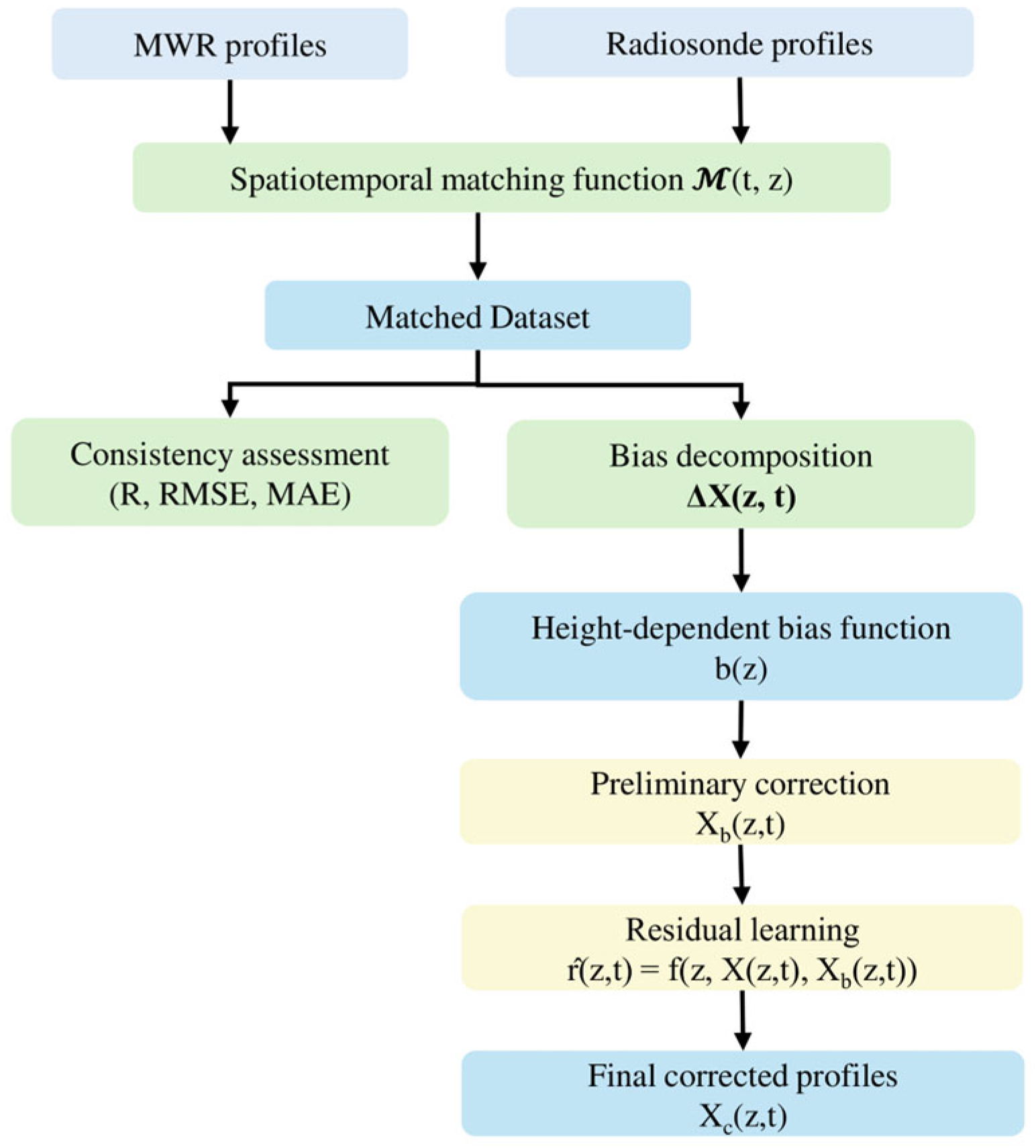
Because microwave-radiometer and radiosonde profiles differ in sampling time and vertical resolution, direct profile-to-profile comparison is insufficient. The MWR and radiosonde profiles were therefore paired using temporal and vertical constraints of Δt ≤ 60 s and Δh ≤ 30 m, respectively. Horizontal distance was not used as an additional filtering criterion because the comparison was conducted within the same Lindenberg observational environment, although representativeness differences associated with radiosonde drift may still contribute to residual uncertainty. Similar collocation-based validation approaches have been used to compare radiosonde, satellite, model, and other independently processed atmospheric profile products [42]. The overall procedure of the MWR–radiosonde thermodynamic consistency correction is summarized in Figure 2.
For a thermodynamic variable X , where X denotes either temperature T or relative humidity R H , the instantaneous difference between the microwave-radiometer retrieval and the matched radiosonde observation was defined as
Δ X ( h , t ) = X M W R ( h , t ) X R S ( h , t )
where h is height, t is observation time, X M W R h , t   is the microwave-radiometer-derived value of variable X at height h and time t , X R S h , t is the matched radiosonde observation of the same variable at height h and time t , and Δ X h , t represents the instantaneous MWR-minus-radiosonde difference. A positive Δ X h , t indicates that the microwave-radiometer retrieval is larger than the corresponding radiosonde observation.
To examine whether the MWR–radiosonde differences contained a systematic vertical component, the instantaneous differences were grouped by height level and averaged over all matched samples. The resulting mean-difference profile was used to represent the systematic height-dependent bias:
b X ( h ) = 1 N h t = 1 N h Δ X ( h , t )
where b X h   is the systematic bias of variable X   at height h , N h   is the number of matched MWR–radiosonde samples available at height h , t indexes the matched samples at that height, and Δ X h , t   is the instantaneous difference defined above. This height-dependent average represents the mean MWR-minus-radiosonde bias at each vertical level. This averaging procedure separates the persistent height-dependent component of the MWR–radiosonde difference from sample-to-sample variability.
The initial bias-corrected thermodynamic variable was obtained as
X b ( h , t ) = X M W R ( h , t ) b X ( h )
where X b ( h , t ) is the thermodynamic variable after systematic bias correction, X M W R h , t   is the original microwave-radiometer-derived value, and b X h   is the systematic height-dependent bias estimated at height h . This correction removes the dominant height-dependent component of the microwave-radiometer retrieval bias.
After this systematic correction, residual differences may remain because retrieval errors can also depend on atmospheric state. The residual term was defined as
r X ( h , t ) = X R S ( h , t ) X b ( h , t )
where r X h , t   is the residual difference after systematic bias correction, X R S h , t   is the matched radiosonde observation, and X b h , t   is the bias-corrected microwave-radiometer value. This residual represents the remaining radiosonde-minus-corrected-MWR difference that is not explained by the height-dependent mean bias.
To represent this remaining state-dependent component, a random forest regressor was trained to estimate the residual using height h , the original microwave-radiometer retrieval X M W R ( h , t ) , and the bias-corrected value X b h , t   as predictors. Tree-based ensemble models are suitable for this residual correction because they can represent nonlinear relationships and interactions among predictors without requiring a prescribed parametric form [43]. To avoid overestimating the correction performance, the residual correction model was evaluated using profile-grouped cross-validation, in which all height levels from the same radiosonde profile were assigned to the same fold.
The final corrected thermodynamic profile was then calculated as
X c ( h , t ) = X b ( h , t ) + r ^ X ( h , t )
where X c h , t   is the final corrected thermodynamic variable, X b h , t   is the value after systematic height-dependent bias correction, and r ^ X h , t   is the residual predicted by the random forest residual model. The corrected thermodynamic variables obtained from the matched MWR–radiosonde samples were used to construct bias-controlled thermodynamic predictors for the subsequent LWC/IWC retrieval experiments. In this study, the correction was estimated and evaluated within the matched-sample framework, because radiosonde observations were required as the reference for calculating MWR–radiosonde differences. The correction procedure was therefore intended to improve the consistency of the thermodynamic predictors used in the collocated retrieval dataset, rather than to generate a complete reprocessed MWR profile product.

2.3.2. Evaluation of Corrected Thermodynamic Profiles

The effectiveness of the thermodynamic correction was evaluated from two complementary perspectives: vertical structural consistency and overall statistical agreement. Vertical consistency was assessed by comparing the mean microwave-radiometer-derived and radiosonde-observed profiles of temperature T and relative humidity RH before and after correction. Statistical agreement was examined using scatter-density distributions and standard validation metrics, including the correlation coefficient r, root mean square error (RMSE), and mean absolute error (MAE). These types of statistical metrics are commonly used to evaluate agreement between retrieved and reference atmospheric profiles [44].
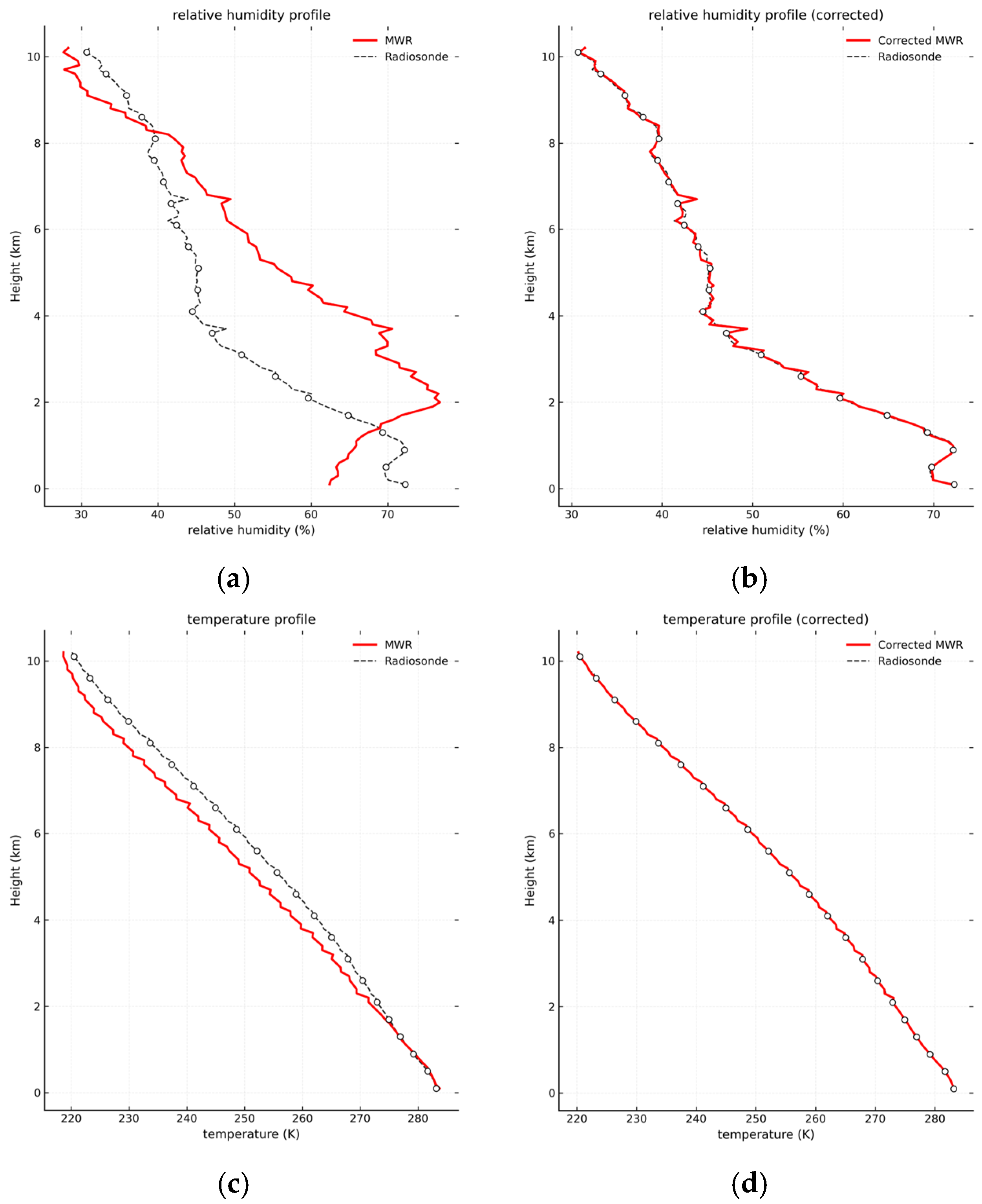
The mean-profile comparisons are shown in Figure 3. Before correction, the microwave-radiometer-derived RH profiles showed clear height-dependent differences from the radiosonde observations, while the temperature profiles also displayed systematic vertical biases. After correction, the mean microwave-radiometer-derived profiles became closer to the corresponding radiosonde profiles, indicating that the dominant height-dependent biases had been reduced. In the mean-profile panels, microwave-radiometer-derived profiles are shown as continuous curves, while radiosonde reference profiles are shown with discrete markers at the matched vertical levels to indicate the difference in vertical sampling.
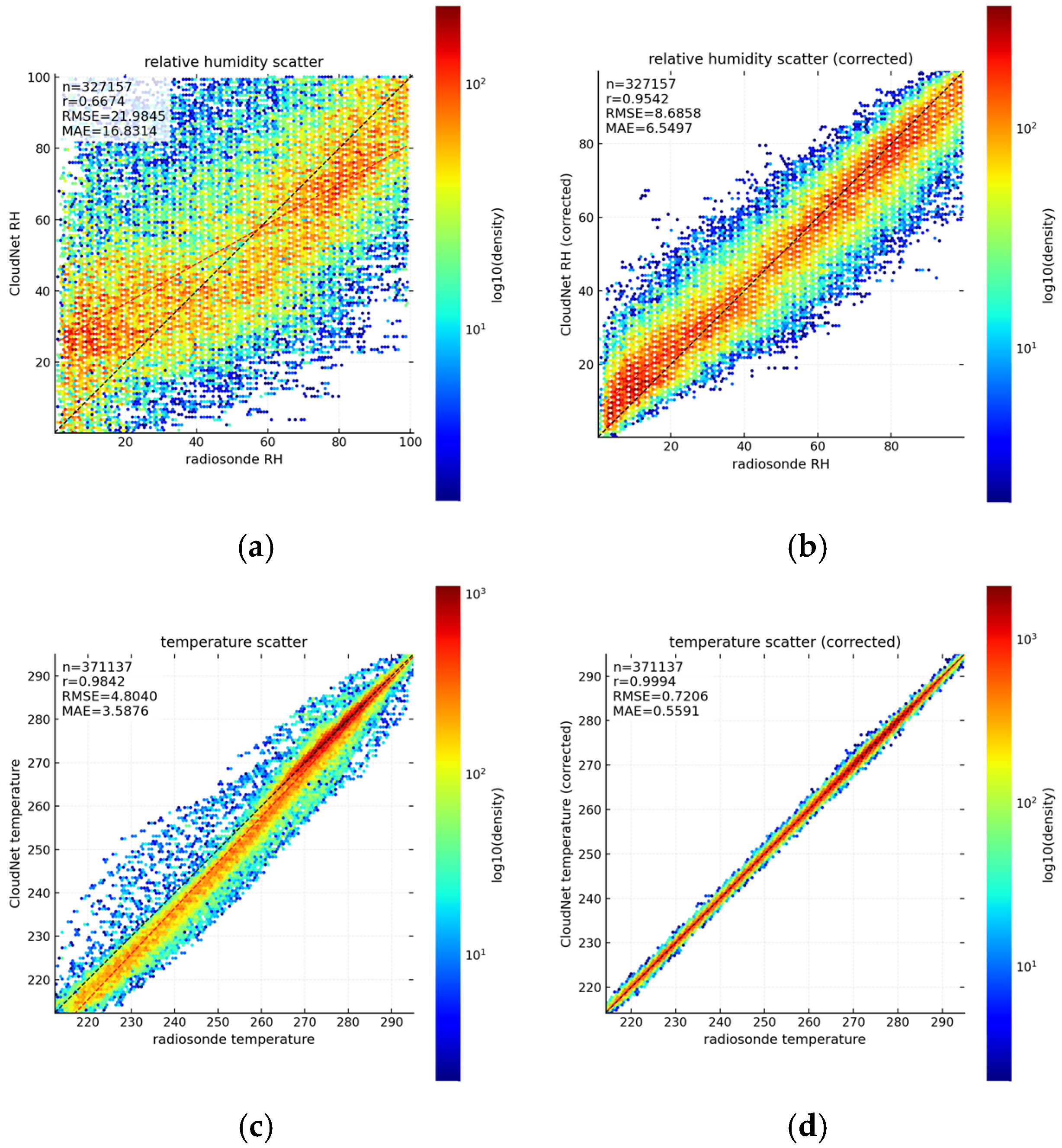
The scatter-density comparisons are shown in Figure 4. Before correction, the microwave-radiometer-derived variables were more widely dispersed around the 1:1 reference line. After correction, the samples became more concentrated along the 1:1 line for both T and RH, indicating improved statistical consistency between the microwave-radiometer and radiosonde observations. This result further confirms that the correction improves not only the mean vertical structure but also the sample-level agreement between the retrieved and reference thermodynamic variables.
The quantitative results are summarized in Table 1. For R H , the correlation coefficient increased from 0.66 to 0.95, while RMSE and MAE decreased from 21.98% and 16.83% to 8.69% and 6.55%, respectively. For T , the correlation coefficient increased from 0.98 to 0.99, while RMSE decreased from 4.80 K to 0.72 K and MAE decreased from 3.58 K to 0.55 K. These results indicate that the correction procedure reduced systematic differences and improved the statistical consistency of the thermodynamic predictors used in the subsequent retrieval model.
The corrected thermodynamic variables were then retained as predictors in the collocated LWC/IWC retrieval dataset. This ensured that the machine-learning framework was trained and evaluated using thermodynamic inputs with reduced systematic differences relative to the radiosonde reference.

2.3.3. Time–Height Collocation of Multisource Observations

To construct collocated multisource samples for LWC and IWC retrieval, Cloudnet-derived LWC and IWC samples were used as the reference coordinates. For each Cloudnet hydrometeor sample, the corresponding radar reflectivity Ze, corrected temperature Tc, and corrected relative humidity RHc were matched in time and height.
A temporal tolerance of Δt ≤ 60 s and a vertical tolerance of Δh ≤ 30 m were applied, where Δt and Δh denote the absolute time and height differences between the Cloudnet hydrometeor sample and the corresponding predictor observation, respectively. Samples that did not satisfy both criteria were excluded, and no additional interpolation or resampling was applied during this step.
The same collocation strategy was applied to the Lindenberg, Munich, and Jülich datasets to maintain consistency between model training, internal testing, and cross-site evaluation. This strict matching strategy reduces mismatch effects in the paired multisource samples, which is important because imperfect temporal and spatial collocation can affect atmospheric-profile comparison statistics [45].

2.3.4. Quality Control

After time–height collocation, quality control was applied to remove samples with missing values, physically implausible thermodynamic conditions, or weak radar signals before model training. The same quality control procedure was applied consistently to cloud radar reflectivity, corrected microwave-radiometer-derived thermodynamic variables, and Cloudnet LWC/IWC products.
Samples with missing target or predictor values were removed. Corrected relative humidity R H c   values greater than 100% were excluded to avoid physically implausible supersaturation artefacts in the microwave-radiometer-derived profiles. Corrected temperature T c   values outside the range of −100 °C to 50 °C were also removed. For radar observations, reflectivity values Z e < 40 dBZ were excluded because such weak signals are more likely to be affected by noise or non-cloud echoes.
This quality control step was intended to construct a reliable paired dataset for supervised learning, rather than to modify the original retrieval products. After filtering, each valid sample contained a Cloudnet LWC or IWC target value and a matched set of predictors, including radar reflectivity Z e , corrected temperature T c , corrected relative humidity R H c , and height.

2.4. Retrieval Dataset Construction

2.4.1. Input Target Sample Definition

After thermodynamic consistency correction, time–height collocation, and quality control, a paired multisource dataset was constructed for LWC and IWC retrieval. Each valid sample represented one matched time–height point and included one Cloudnet-derived hydrometeor target value together with the corresponding radar and thermodynamic predictors.
For each matched sample, the basic input vector was defined as
x ( h , t ) = Z e ( h , t ) , T c ( h , t ) , R H c ( h , t ) , h
where x ( h , t ) is the input feature vector at height h   and time t , Z e ( h , t ) is the matched cloud radar reflectivity, T c h , t   is the corrected temperature profile, R H c h , t   is the corrected relative humidity profile.
The supervised learning targets were defined separately for LWC and IWC:
y L W C ( h , t ) = L W C ( h , t )
y I W C ( h , t ) = I W C ( h , t )
where y L W C h , t   and y I W C h , t   are the supervised learning targets for liquid water content and ice water content, respectively. L W C ( h , t ) and I W C ( h , t ) are the Cloudnet-derived liquid and ice water content products at height h   and time t , respectively.
In this study, LWC and IWC were treated as two separate regression tasks. The same data construction and feature-generation procedure was applied to both variables, but independent models were trained for each target. This is because LWC and IWC differ in their vertical distributions, statistical properties, and controlling physical processes. This design maintains methodological consistency while allowing each model to capture the specific behaviour of its target variable.
This independent-target formulation also introduces a limitation in mixed-phase conditions. In mixed-phase cloud regions, radar reflectivity and thermodynamic variables may contain coupled sensitivity to both liquid and ice hydrometeors. Therefore, separate LWC and IWC models do not explicitly enforce liquid–ice coexistence or phase-partitioning constraints, and the independently retrieved values may occasionally produce physically inconsistent liquid–ice combinations, particularly near the melting layer or under temperature conditions where supercooled liquid droplets and ice particles coexist. This uncertainty should be considered when interpreting mixed-phase retrieval results. In the present framework, such uncertainty is mainly reflected in the residual errors of the independently trained LWC and IWC models. A joint multi-output retrieval strategy or a physics-constrained learning framework with temperature-dependent phase constraints would be a useful extension in future work.

2.4.2. Logarithmic Transformation of LWC/IWC Targets

Both LWC and IWC are non-negative variables and usually have strongly skewed distributions, with many small values and a smaller number of large values. If regression is performed directly in the original physical space, large hydrometeor values may dominate model training and reduce the model’s sensitivity to weaker cloud signals. To improve numerical stability and limit the influence of extreme values, the target variables were transformed into logarithmic space before model training. Similar logarithmic transformations have been used in cloud-water retrieval studies to handle right-skewed target distributions [46].
Before transformation, hydrometeor content was converted from g m−3 to mg m−3:
W m g ( h , t ) = 10 3 W ( h , t )
where W ( h , t ) denotes either LWC or IWC in g m−3, and W m g ( h , t ) is the corresponding hydrometeor content in mg m−3.
The transformed learning target was then defined as
y ( h , t ) = l n 1 + W m g ( h , t )
The constant term prevents undefined logarithmic values when hydrometeor content is zero. This logarithmic transformation compresses the dynamic range of the target variable and shifts the learning emphasis from large absolute errors toward relative variations across both weak and strong hydrometeor signals.
During inference, the predicted value in logarithmic space was transformed back to the physical domain as
W ^ m g ( h , t ) = e x p y ^ ( h , t ) 1
The predicted hydrometeor content was then converted back to g m−3:
W ^ ( h , t ) = W ^ m g ( h , t ) 1000
where y ^ ( h , t ) is the model prediction in logarithmic space, W ^ m g ( h , t ) is the predicted hydrometeor content in mg m−3, and W ^ ( h , t ) is the final predicted LWC or IWC value in g m−3.

2.4.3. Height-Dependent Dataset Characterization

Cloud liquid and ice water contents show clear height-dependent behaviour. In the processed Lindenberg dataset, IWC samples were mainly distributed in the middle and upper troposphere, whereas LWC samples were concentrated in the lower troposphere. This contrast indicates that the two variables are associated with different vertical regimes and that their distributions should be examined with height dependence in mind.
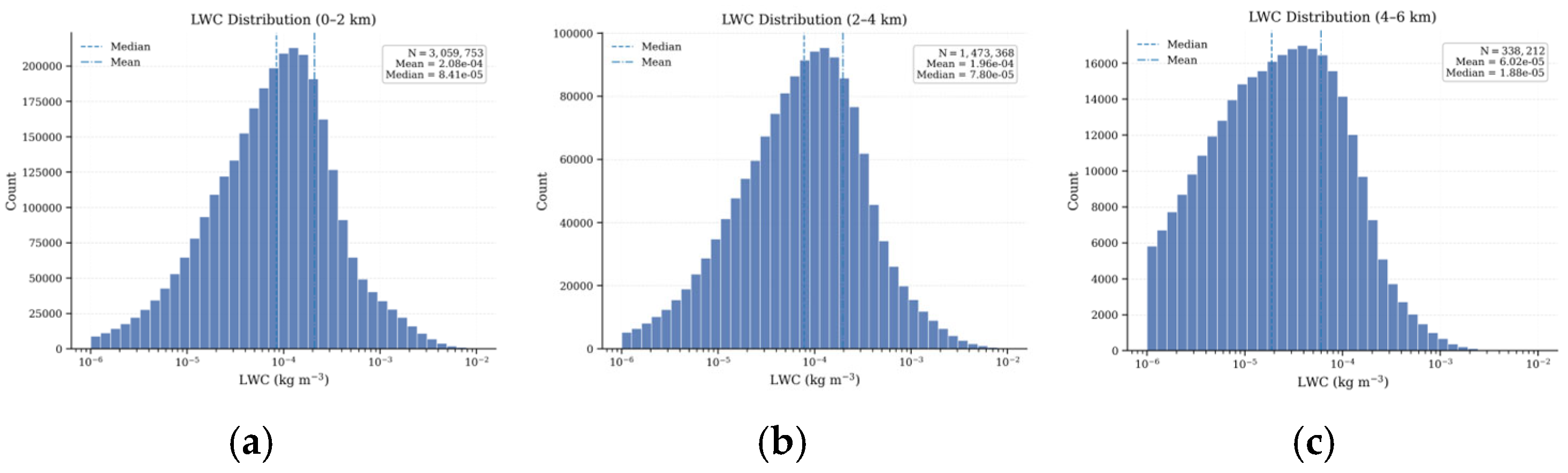
To characterize this vertical variability, the processed samples were grouped into predefined altitude ranges. For IWC, the altitude intervals were 0–3 km, 3–6 km, and 6–9 km. For LWC, the altitude intervals were 0–2 km, 2–4 km, and 4–6 km. These altitude intervals were used to describe the main vertical distribution of the available samples and to support height-dependent interpretation of the retrieval results. The detailed distribution plots are provided in Appendix A rather than in the main text because their purpose is to document dataset characteristics rather than to support the main methodological contribution.
The 0–9 km range was used as the primary altitude range for IWC distribution characterization because it covers the dominant portion of the available IWC samples and allows the vertical distribution to be compared across low-, middle-, and upper-tropospheric layers with sufficient sample support. To further examine the representation of higher-level ice clouds, the altitude coverage of the available Cloudnet IWC records was additionally checked. A total of 4,911,349 valid IWC records were located above 9 km, accounting for 11.02% of all valid IWC records considered in the altitude-coverage analysis. This indicates that high-altitude IWC samples were present in the dataset and should not be neglected. However, the majority of the valid IWC records were still located below 9 km, and the 0–9 km range therefore provides a stable basis for summarizing the main IWC distribution in the present analysis. High-level ice clouds, such as cirrus clouds and deep convective anvils, can extend above 9 km in the mid-to-upper troposphere. Therefore, retrieval performance for upper-tropospheric ice clouds should be interpreted with caution and warrants more detailed height-resolved evaluation in future work.
The relatively high mean IWC value in the 0–3 km layer should also be interpreted cautiously. Low-level IWC samples may be affected by mixed-phase hydrometeors, melting-layer particles, phase-classification uncertainty in the reference product, and a small number of extreme values. These factors can increase the mean IWC value in the lower troposphere and may partly explain why the mean IWC in the 0–3 km layer is comparable to that in the 3–6 km layer. This does not necessarily indicate that low-level ice is generally more abundant than mid-level ice, but rather reflects the sensitivity of layer-mean statistics to phase ambiguity and outliers in the processed reference dataset. Therefore, the reliability of low-level IWC retrieval should be considered with caution, especially in mixed-phase and melting-layer conditions.
These altitude intervals were used only for dataset characterization and height-dependent evaluation. They were not used to build separate retrieval models for individual altitude ranges. Unless otherwise stated, one unified retrieval framework was trained for each target variable, with height and vertical-structure descriptors included in the predictor space. This design allows the model to learn height-dependent relationships while maintaining a consistent profile-level retrieval formulation.

2.4.4. Training, Testing, and Independent Site Datasets

The Lindenberg dataset was used for model training and internal evaluation. After preprocessing and logarithmic target transformation, the valid Lindenberg profiles were divided into training and testing subsets at a 4:1 ratio using the atmospheric profile index as the grouping unit. The partitioning strategy was a profile-level grouped split, rather than a random split of individual time–height samples. All height levels belonging to the same atmospheric profile were assigned to the same subset, so samples from the same vertical profile did not appear simultaneously in both the training and testing subsets.
This profile-level split was used to reduce the risk of data leakage caused by vertical dependence within cloud profiles. If individual height gates from the same profile were randomly distributed between training and testing subsets, neighbouring samples with similar radar, thermodynamic, and hydrometeor structures could lead to overly optimistic evaluation results. Therefore, the reported internal testing performance, including the high correlation values, was not obtained from a height-gate-level random split. No stratified sampling or time-series cross-validation was used in the internal Lindenberg experiment, and the same profile-level partition was applied to all model configurations to ensure fair comparison.
After time–height matching and quality control, the final Lindenberg dataset contained 457,940 valid paired samples for IWC retrieval and 244,950 valid paired samples for LWC retrieval. Each sample included a Cloudnet-derived LWC or IWC target value and the corresponding matched predictors, including radar reflectivity Ze, corrected temperature Tc, corrected relative humidity RHc, and height h.
For model comparison and ablation experiments, the same training–testing partition was used for all model configurations. This ensured that performance differences mainly reflected changes in model structure, input variables, or vertical-structure modules, rather than differences in data splitting.
For cross-site evaluation, the Munich and Jülich datasets were processed using the same collocation, quality-control, target-transformation, and feature-construction procedures as the Lindenberg dataset. These datasets were not used for model training, hyperparameter selection, or model refinement. Models trained on Lindenberg were applied directly to Munich and Jülich without retraining, fine-tuning, or site-specific parameter adjustment. This design provides an independent cross-site evaluation of whether the learned relationships among radar reflectivity, thermodynamic structure, vertical features, and Cloudnet-derived cloud water content can transfer across different observational environments.
The internal Lindenberg evaluation used Cloudnet-derived LWC and IWC products as both training targets and testing references. Therefore, although the profile-level split reduces direct leakage between vertically adjacent samples from the same profile, the internal evaluation is still based on reference products from the same processing framework. The Munich and Jülich experiments partly address this limitation by testing the Lindenberg-trained models at independent sites. However, because the reference LWC and IWC products at these sites are also derived from the Cloudnet processing framework, the cross-site evaluation should not be interpreted as fully independent in situ microphysical validation. Such validation would require aircraft measurements or other independent LWC/IWC profile products, which were not available in the present study.

2.5. Vertically Structured Retrieval Framework

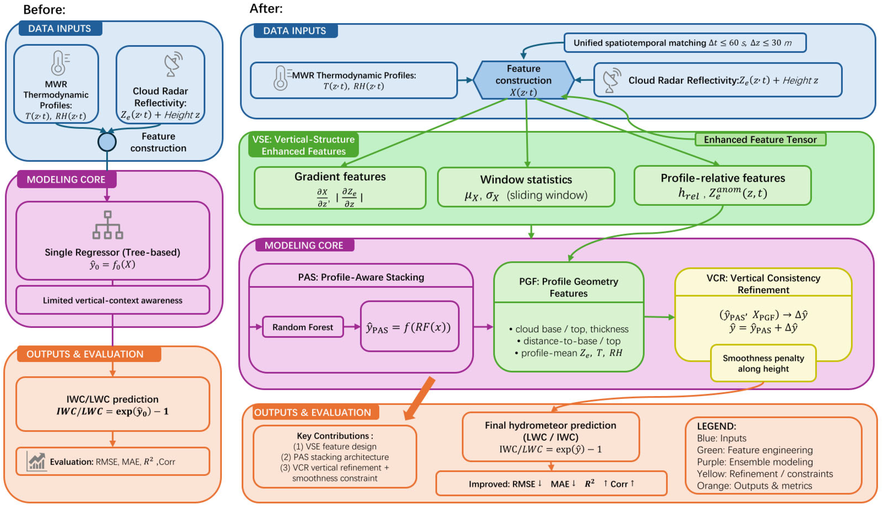
Figure 5 illustrates the conceptual difference between the baseline pointwise retrieval model and the proposed vertically structured framework. The baseline model treats each height level as an independent sample and predicts LWC or IWC using only single-level predictors, including cloud radar reflectivity Z e , thermodynamic variables, and height. In contrast, the proposed framework incorporates vertical-structure-enhanced features, profile-aware stacking, a profile grouping framework based on cloud geometry, and vertical consistency refinement to better represent the profile-level organization of cloud water content. The following subsections describe these components in detail.

2.5.1. Baseline Pointwise Random-Forest Retrieval

The baseline retrieval model was built using pointwise random forest regression. In this configuration, each matched time–height sample was treated as an independent training sample. The model used the single-level predictors defined in Section 2.4.1 to estimate LWC or IWC at the corresponding height.
The baseline pointwise retrieval was expressed as
y ^ ( h , t ) = f R F x ( h , t )
where x h , t   is the input feature vector at height h and time t , f R F ( ) denotes the random forest regression function, and y ^ ( h , t ) is the predicted hydrometeor content in logarithmic space. The predicted logarithmic value y ^ ( h , t ) was subsequently transformed back to the physical hydrometeor content following the inverse transformation described in Section 2.4.2.
Random forest was selected as the baseline because tree-based ensemble models can capture nonlinear relationships among radar reflectivity, thermodynamic variables, and height without requiring a predefined analytical form. This is useful for LWC/IWC retrieval because the relationship between cloud water content, radar reflectivity, and thermodynamic conditions is nonlinear and varies across cloud regimes.
However, the pointwise baseline does not explicitly represent the vertical structure of cloud profiles. Although the height coordinate is included as an input variable, each height level is still predicted separately. As a result, neighbouring levels within the same atmospheric profile are not directly constrained to be vertically consistent. Previous atmospheric profile retrieval studies have shown that neighbouring variables within a vertical profile are correlated, indicating that profile structure should not be ignored in retrieval modelling [47]. Treating height levels independently may also introduce localized artificial oscillations in retrieved profiles [48].
This limitation motivates the vertically structured framework described below. Rather than replacing the random forest baseline with a different model family, the proposed framework extends it by incorporating vertical-context features, profile-aware ensemble learning, and profile-level consistency refinement.

2.5.2. Vertical-Structure-Enhanced Features

Vertical-structure-enhanced features were introduced to provide the model with information about the local vertical environment around each sample. This design is based on the fact that cloud radar reflectivity, temperature, relative humidity, LWC, and IWC often vary coherently with height, while sharp transitions may occur near cloud boundaries and phase-change regions. These vertical patterns cannot be fully represented by single-level predictors alone.
For each profile, samples were first sorted by height. Vertical gradients of the key predictors were then calculated using neighbouring height levels. For a variable X , where X   represents Z e , T , or R H , the vertical gradient at height h i was approximated as
X z ( h i , t ) = X ( h i + 1 , t ) X ( h i 1 , t ) h i + 1 h i 1
For boundary levels, forward or backward differences were used. Because the Cloudnet profiles used in this study are provided on an approximately regular vertical grid with a nominal spacing of about 30 m, this finite-difference approximation provides a practical measure of local vertical variation.
The radar reflectivity gradient was included because strong changes in reflectivity are often associated with cloud boundaries, hydrometeor transitions, or phase-change regions. The gradient magnitude of radar reflectivity was defined as
G Z e ( h i , t ) = Z e h ( h i , t )
where G Z e ( h i , t ) represents the local magnitude of vertical reflectivity change. Large values indicate sharp vertical transitions in cloud structure.
To reduce the influence of local noise and describe the surrounding vertical context, sliding-window statistics were also calculated. For a fixed vertical neighbourhood Ω i   centred on height h i , the local mean of variable X   was defined as
μ X ( h i , t ) = 1 Ω i j Ω i X ( h j , t )
and the corresponding local variability was defined as
σ X ( h i , t ) = 1 Ω i j Ω i X ( h j , t ) μ X ( h i , t ) 2
Here, Ω i denotes the local vertical window centred on height h i , and Ω i is the number of valid height levels included in this window. The index j denotes a neighbouring height level within Ω i , and h j is the corresponding height. X ( h j , t ) is the value of variable X at height h j and time t. μ X ( h i , t ) represents the local mean of X within Ω i , while σ X ( h i , t ) represents the corresponding local standard deviation. In this study, a fixed window of ±3 height levels was used, corresponding to an approximate vertical span of 180 m.
In addition, profile-relative descriptors were introduced to help the model identify the position of each sample within the vertical column. The normalized relative height was defined as
h r e l ( h i , t ) = h i h m i n ( t ) h m a x ( t ) h m i n ( t )
where hi denotes the height of the i -th valid sample in the profile at time t, hmin(t) and hmax(t) denote the minimum and maximum valid heights of that profile, respectively, and hrel(hi, t) is the normalized relative height of the sample within the vertical column.
A reflectivity anomaly term was also used to describe the deviation of each height level from the column-mean radar reflectivity:
h a n o m ( h i , t ) = Z e ( h i , t ) Z e ( t )
where Z e ( t ) is the mean radar reflectivity over all valid height levels in the profile at time t .
The final VSE-enhanced feature vector was therefore defined as
x V S E h i , t = x h i , t , Z e h , T c h , R H c h , G Z e , μ X , σ X , h r e l , h a n o m
where x V S E h i , t is the vertical-structure-enhanced feature vector at height level h i and time t , and x h i , t is the original single-level input vector. The terms Z e / h , T c / h , and R H c / h represent the vertical gradients of radar reflectivity, corrected temperature, and corrected relative humidity, respectively. G Z e denotes the magnitude of the vertical reflectivity gradient. X denotes any of the three predictor variables Z e , T c , or R H c , so μ X and σ X represent the sliding-window local mean and local standard deviation of these predictors. h r e l is the normalized relative height, and h a n o m is the radar reflectivity anomaly relative to the profile-mean reflectivity.

2.5.3. Profile-Aware Stacking of Tree-Based Learners

After the vertical-structure-enhanced features were constructed, a profile-aware stacking strategy was introduced to improve model robustness. This step was designed to reduce dependence on a single random forest configuration and to improve generalization across cloud regimes with different vertical structures.
The stacking framework used K   base learners. In this study, K = 5 random forest base learners were trained with different hyperparameter settings to increase diversity among their predictions. The base learners used different combinations of tree number and maximum tree depth:
( n t r e e s , d m a x ) { ( 100,10 ) , ( 200,15 ) , ( 300,20 ) , ( 400,25 ) , ( 500,30 ) }
where n t r e e s is the number of trees in a random forest base learner, d m a x is the maximum tree depth, and each pair n t r e e s d m a x defines one base-learner configuration. This design allows different base learners to represent patterns of varying complexity and increases diversity among their predictions.
For the k -th base learner, the prediction was defined as
y ^ k ( h i , t ) = f k x V S E ( h i , t ) , k = 1,2 , , K
where k   is the base-learner index, K   is the total number of base learners, f k ( ) denotes the k -th random forest base learner, x V S E ( h i , t ) is the vertical-structure-enhanced feature vector at height level h i   and time t , and y ^ k ( h i , t ) is the logarithmic-space prediction produced by the k -th base learner.
The predictions from all base learners were then combined into a second-level feature vector:
h ( h i , t ) = y ^ 1 ( h i , t ) , y ^ 2 ( h i , t ) , , y ^ K ( h i , t )
where h ( h i , t ) is the second-level stacking feature vector, and y ^ 1 ( h i , t ) , y ^ 2 ( h i , t ) , , y ^ K ( h i , t ) are the logarithmic-space predictions from the K random forest base learners.
A ridge regression meta-learner was used to combine the base-learner outputs:
y ^ P A S ( h i , t ) = f r i d g e h ( h i , t )
where f r i d g e denotes the ridge regression meta-learner, h ( h i , t ) is the second-level feature vector constructed from the base-learner predictions, and y ^ P A S ( h i , t ) is the profile-aware stacking prediction in logarithmic space.
Ridge regression was selected because predictions from different tree-based learners may be correlated. Its regularization term stabilizes the meta-learner and reduces the risk of overfitting to any single base-learner configuration.
To avoid information leakage between training and validation samples, grouped cross-validation was applied using the atmospheric profile as the grouping unit. All height levels from the same profile were assigned to the same fold. This design ensures that validation performance reflects generalization to unseen profiles, rather than benefiting from partial overlap among height levels within the same profile.
Through this profile-aware stacking strategy, the model combines complementary predictions from multiple tree-based learners while preserving the profile structure of the data. This improves robustness across heterogeneous cloud regimes and reduces variance-driven instability in the retrieval results.

2.5.4. Profile Grouping Framework Based on Cloud Geometry and Vertical Consistency Refinement

Although VSE and PAS introduce vertical context and improve model robustness, predictions are still generated at individual height levels. As a result, some retrieved profiles may appear locally reasonable but remain vertically inconsistent, especially near cloud boundaries or phase-transition regions. To address this issue, a profile grouping framework based on cloud geometry (PGF) and vertical consistency refinement (VCR) was applied at the profile level.
First, the effective cloud echo region was identified using a radar reflectivity threshold. In this study, a threshold of approximately −40 dBZ was used to define valid cloud echoes. This value is close to the nominal sensitivity range of Ka-band cloud radars such as MIRA-35 under typical operating conditions and helps reduce the influence of noise-dominated radar signals.
For each profile at time t , the cloud-base height and cloud-top height were defined as
h b t = min h : Z e h , t Z t h
h t t = max h : Z e h , t Z t h
where Z t h   is the reflectivity threshold, h b ( t ) is the cloud-base height, and h t ( t ) is the cloud-top height.
Cloud thickness was then defined as
H c ( t ) = h t ( t ) h b ( t )
The distances from each height level to the cloud base and cloud top were defined as
d b ( h , t ) = h h b ( t )
d t ( h , t ) = h t ( t ) h
These cloud-geometry variables describe the relative position of each sample within the cloud layer and provide information that cannot be fully captured by absolute height alone. These cloud-geometry variables provide explicit cloud-boundary information, such as cloud-base height and cloud thickness, that can be added to atmospheric profile retrieval as auxiliary predictors [49].
Using the cloud-geometry-enhanced feature space, the PAS prediction was treated as the initial profile estimate:
y ^ 0 ( h , t ) = y ^ P A S ( h , t )
A residual refinement term was then introduced:
y ^ f i n a l ( h , t ) = y ^ 0 ( h , t ) + r ^ ( h , t )
where r ^ ( h , t ) is the predicted residual correction.
The reference residual was defined as
r ( h , t ) = y ( h , t ) y ^ 0 ( h , t )
A separate random forest regressor was trained to estimate this residual using the VSE features and cloud-geometry descriptors. To reduce overfitting, the residual model was configured to be shallower than the main ensemble model.
Because pointwise predictions may produce unrealistic layer-to-layer oscillations, a lightweight vertical refinement step was applied after residual prediction. The residual was first estimated using the random forest residual model, and the preliminary corrected profile was obtained by adding the predicted residual to the PAS prediction.
To reduce isolated small-scale fluctuations, the final profile was smoothed along the vertical dimension using neighbouring height levels. This refinement was applied only as a post-processing step and was not used to train the random forest residual model. Its purpose was to suppress local oscillations that were inconsistent with the surrounding vertical structure while preserving physically meaningful sharp gradients near cloud boundaries.
In this study, the vertical refinement was implemented sequentially: the residual model first learned the difference between the Cloudnet reference value and the PAS prediction, and the resulting profile was then refined along the vertical dimension. This design improves profile-level coherence without requiring joint optimization of a custom loss function.
Through this design, the PGF variables and VCR step act on the retrieved profile after the pointwise prediction stage. They complement VSE and PAS by improving the structural coherence of the final LWC/IWC profiles.

2.6. Experimental Design and Evaluation Metrics

2.6.1. Baseline Model Comparison

To evaluate the effectiveness of the proposed vertically structured retrieval framework, several representative regression models were used as baselines. These included multiple linear regression, multilayer perceptron (MLP), long short-term memory network (LSTM), random forest, extra trees, and histogram-based gradient boosting. Together, these models cover linear regression, neural-network-based regression, and tree-based ensemble learning, allowing the proposed framework to be compared with methods that differ in complexity and representational ability.
All models were trained and evaluated using the same matched dataset, input variables, target definitions, and training–testing split. This ensured that performance differences mainly reflected the modelling strategy, rather than differences in data partitioning or preprocessing. For the LSTM baseline, vertically ordered samples from the same atmospheric profile were treated as one input sequence, and the profile-level training–testing split was retained to prevent information leakage between training and testing sequences. The baseline comparison was used to assess whether explicitly incorporating vertical structure improves retrieval performance beyond conventional pointwise or general-purpose machine-learning models. A recent atmospheric-profile retrieval study compared multiple machine-learning algorithms under a consistent observational dataset and validation framework [50].
The hyperparameter configurations of the baseline models are summarized in Table 2.

2.6.2. Input-Variable Ablation Design

Input-variable ablation experiments were conducted to examine the contribution of different predictor groups to LWC and IWC retrieval. Starting from the full predictor set, individual variables or variable groups were removed to assess their influence on model performance. The tested predictor groups included radar reflectivity Z e , corrected temperature T c , corrected relative humidity R H c , and height-related information.
In this study, height-related information included the original height coordinate and explicitly height-dependent descriptors, such as normalized relative height and cloud-geometry descriptors. When height-related information was removed, these variables were excluded from the corresponding ablation configuration, while radar reflectivity and thermodynamic predictors were retained. Therefore, the “without height” experiment was designed to evaluate the effect of removing explicit vertical positional information from an otherwise multisource retrieval model.
Two additional single-source configurations were included to provide simple reference baselines: a height-only configuration and a radar-only configuration. In the height-only configuration, only height-related variables were retained, while radar reflectivity, corrected temperature, and corrected relative humidity were excluded. This configuration was not intended to represent a physically complete retrieval model, but rather to evaluate how much of the target variability could be explained by the climatological vertical background alone. In the radar-only configuration, only radar reflectivity was retained, while thermodynamic and height-related variables were excluded. This setting was used to assess the information content of radar-observed cloud echo structure alone.
These single-source configurations were kept separate from the “without height” configuration. Specifically, “without height” retains radar reflectivity and thermodynamic predictors but removes explicit vertical positional information, whereas “height-only” and “radar-only” use only one category of predictor. This distinction allows the ablation experiments to separate the effects of radar-observed cloud structure, thermodynamic state, and vertical-context information. The purpose of this design was not to suggest that any single predictor group is sufficient for reliable LWC or IWC retrieval, but to evaluate how different sources of information contribute to the performance of the full vertically structured framework.

2.6.3. Stepwise Module Ablation Design

A second set of ablation experiments was conducted to evaluate the contribution of each component in the proposed vertically structured retrieval framework. Starting from the baseline random forest model, the framework was progressively extended by adding vertical-structure-enhanced features, profile-aware stacking, the profile grouping framework based on cloud geometry, and vertical consistency refinement.
This stepwise design was used to separate the effects of vertical feature construction, ensemble integration, cloud-geometry information, and profile-level consistency refinement. It also helped distinguish the contribution of vertical contextual information from improvements caused by increased model complexity or ensemble averaging.

2.6.4. Boundary-Region Evaluation Design

To provide a more targeted assessment of retrieval performance near cloud boundaries, an additional boundary-region evaluation was conducted using the Lindenberg testing dataset. This evaluation was designed to examine whether the proposed vertically structured framework improves retrieval performance in regions where cloud water content and radar reflectivity may change rapidly with height.
Cloud-boundary regions were identified using the radar-reflectivity-based cloud geometry definition introduced in Section 2.5.4. For each atmospheric profile, valid cloud echoes were first identified using a radar reflectivity threshold of −40 dBZ. The cloud-base height and cloud-top height were then defined as the lowest and highest height levels, respectively, at which radar reflectivity exceeded this threshold. Profiles without valid radar echoes above this threshold were excluded from the boundary-region evaluation because cloud base and cloud top could not be defined reliably.
For each valid in-cloud sample, the distance to the nearest cloud boundary was calculated as the minimum distance to either the cloud base or the cloud top. Samples located within three radar range gates, approximately 90 m, from either cloud base or cloud top were classified as near-boundary samples. The remaining in-cloud samples were classified as cloud-interior samples. The boundary width of 90 m was selected because the vertical resolution of the cloud radar profiles is approximately 30 m, so this threshold corresponds to about three vertical range gates.
The baseline random forest model and the proposed framework were then evaluated separately in the near-boundary and cloud-interior regions for both IWC and LWC retrieval. The same testing samples and evaluation metrics were used for both models to ensure a fair comparison. This region-specific analysis complements the overall and height-dependent evaluations by directly assessing model performance in cloud regions where vertical gradients and boundary effects are expected to be more important.

2.6.5. Cross-Site Evaluation Strategy

To assess the transferability of the proposed retrieval framework, an independent cross-site evaluation was conducted using observations from the Munich and Jülich Cloudnet sites. The retrieval models were trained only on the Lindenberg dataset and then applied directly to the Munich and Jülich datasets without retraining, fine-tuning, or site-specific parameter adjustment.
For cross-site evaluation, the thermodynamic correction model derived from the Lindenberg MWR–radiosonde matched dataset was applied to the thermodynamic predictor samples from Munich and Jülich without site-specific retraining. The Munich and Jülich datasets were then processed using the same general preprocessing and feature-construction procedures as the Lindenberg dataset, including time–height collocation, quality control, logarithmic target transformation, and inverse transformation of the predicted LWC/IWC values. The cross-site datasets were not used for model training, hyperparameter selection, thermodynamic correction model fitting, or retrieval-model refinement. This ensured that performance differences mainly reflected changes in observational conditions and cloud-regime characteristics rather than differences in model adjustment or data partitioning.
The cross-site experiment was designed to test whether the relationships learned from Lindenberg among radar reflectivity Z e , corrected thermodynamic structure, vertical features, and Cloudnet-derived LWC/IWC products could be transferred to independent sites. Performance was evaluated using the same metrics as in the internal evaluation, including MAE, RMSE, correlation coefficient, and coefficient of determination R 2 .

2.6.6. Evaluation Metrics

Model performance was evaluated using four commonly used statistical metrics: the root mean square error (RMSE), mean absolute error (MAE), coefficient of determination (R2), and Pearson correlation coefficient. These metrics were used to quantify the absolute retrieval error, explained variance, and linear agreement between the retrieved and reference LWC/IWC values. Because these metrics are widely used in atmospheric-profile retrieval evaluation, their mathematical formulations are not repeated here.

3. Results

The performance of the proposed framework for retrieving cloud liquid water content (LWC) and ice water content (IWC) is evaluated using year-round observations from the Cloudnet Lindenberg site in 2025. The target variables are obtained from the Cloudnet LWC and IWC profile products, while the input features include METEK MIRA-35 radar reflectivity (Ze) and bias-corrected thermodynamic profiles of temperature and relative humidity derived from the Cloudnet microwave radiometer.
After applying unified time–height matching and quality control procedures, multisource paired datasets are constructed. The resulting dataset contains 457,940 valid samples for IWC and 244,950 samples for LWC. The valid atmospheric profiles were divided into training and testing subsets at a ratio of 4:1 using the profile index as the grouping unit, ensuring that all height levels from the same profile were assigned to the same subset.
Model performance is assessed using root mean square error (RMSE), mean absolute error (MAE), correlation coefficient (Corr), and coefficient of determination (R2). The following sections present comparisons across different models, examine height-dependent retrieval behavior, and analyze the contributions of individual variables and model components through ablation experiments.

3.1. Overall Performance Evaluation on the Year-Round Dataset

The predictive performance of different machine-learning models is summarized in Table 3 (IWC) and Table 4 (LWC).
For the IWC retrieval task, the multiple linear regression (MLR) model performs poorly (R2 = −0.105), indicating that a linear mapping cannot represent the nonlinear relationships between thermodynamic conditions, radar reflectivity, and ice microphysical variability. Ice microphysics involves nonlinear processes such as the exponential dependence of saturation vapor pressure on temperature and the power-law relationship between radar reflectivity and hydrometeor mass.
The multilayer perceptron (MLP) increases R2 to 0.060, but the improvement remains limited because it treats each height level independently and ignores vertical structural dependence. The LSTM model achieves R2 = 0.079, but the gain remains modest because the retrieval problem is formulated as pointwise regression rather than sequential prediction, preventing the recurrent architecture from exploiting sequence-learning capability.
Tree-based ensemble models perform substantially better. The Random Forest baseline increases R2 to 0.412 and reduces RMSE to 0.0152, indicating that nonlinear feature partitioning effectively captures interactions among thermodynamic variables and radar observations.
The proposed framework further improves performance, reducing RMSE to 0.0092 and increasing R2 to 0.784. These gains demonstrate that encoding vertical structure through VSE, together with profile-level refinement via PAS and VCR, enables the model to represent vertically coherent cloud processes rather than treating each level independently.
For LWC retrieval, overall performance is lower than for IWC. The Random Forest baseline achieves R2 = 0.303, whereas the proposed method increases R2 to 0.606 and reduces RMSE from 0.0786 to 0.0591 g m−3.
This difference reflects the physical nature of liquid clouds. LWC is strongly influenced by boundary-layer turbulence, aerosol activation, and rapid phase transitions, which introduce substantial small-scale variability. By incorporating vertical-structure features, the proposed framework distinguishes different cloud regimes, enabling more accurate retrieval of liquid-water variability.
While the above analysis focuses on overall performance aggregated across all height levels, cloud microphysical properties and retrieval difficulty exhibit strong vertical heterogeneity. To further characterize retrieval behavior, the following section examines how model performance varies with altitude.

3.2. Height-Dependent Performance Evaluation

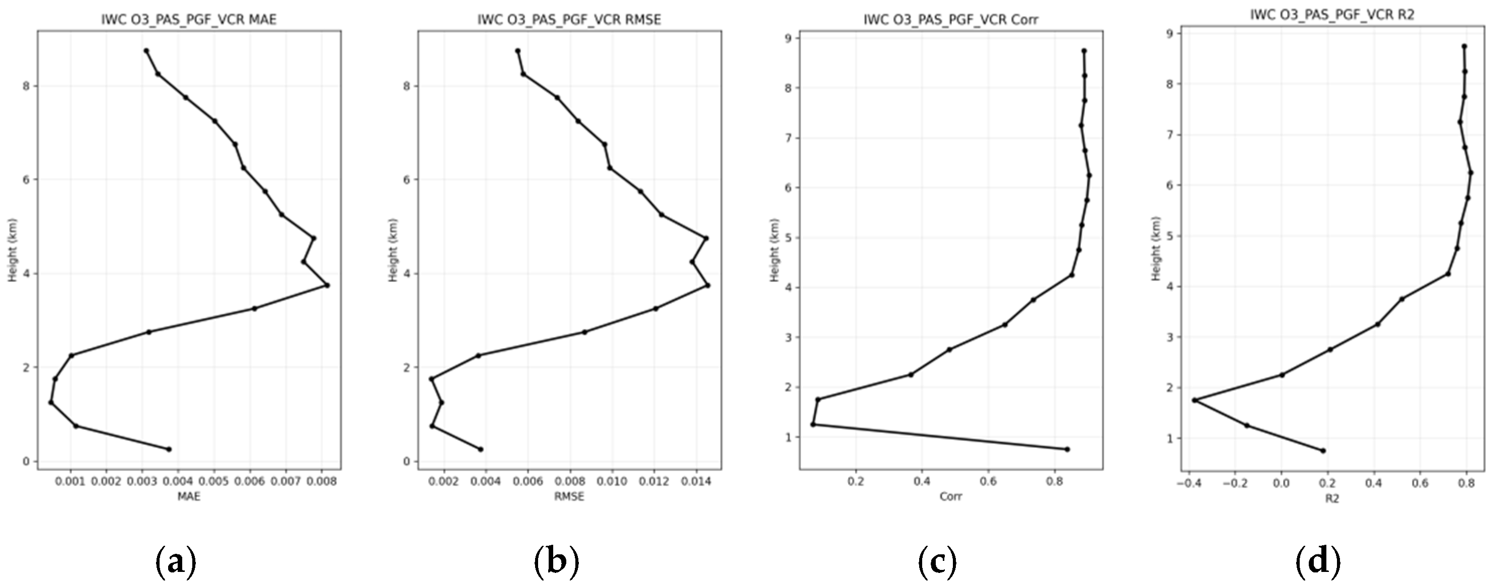
The height-dependent performance metrics for IWC retrieval are summarized in Table 5. In the 0–3 km layer, the model exhibits small absolute errors but explains limited variance due to the sparse occurrence of ice water content and mixed-phase processes.
Retrieval accuracy improves substantially in the 3–6 km and 6–9 km layers, where upper-tropospheric ice clouds exhibit more stable particle-size distributions, producing clearer relationships between reflectivity, thermodynamic structure, and IWC.
The vertical evolution of these metrics is illustrated in Figure 6, where error metrics decrease with height while correlation metrics increase, indicating that the framework performs best in regimes with coherent vertical cloud structure.
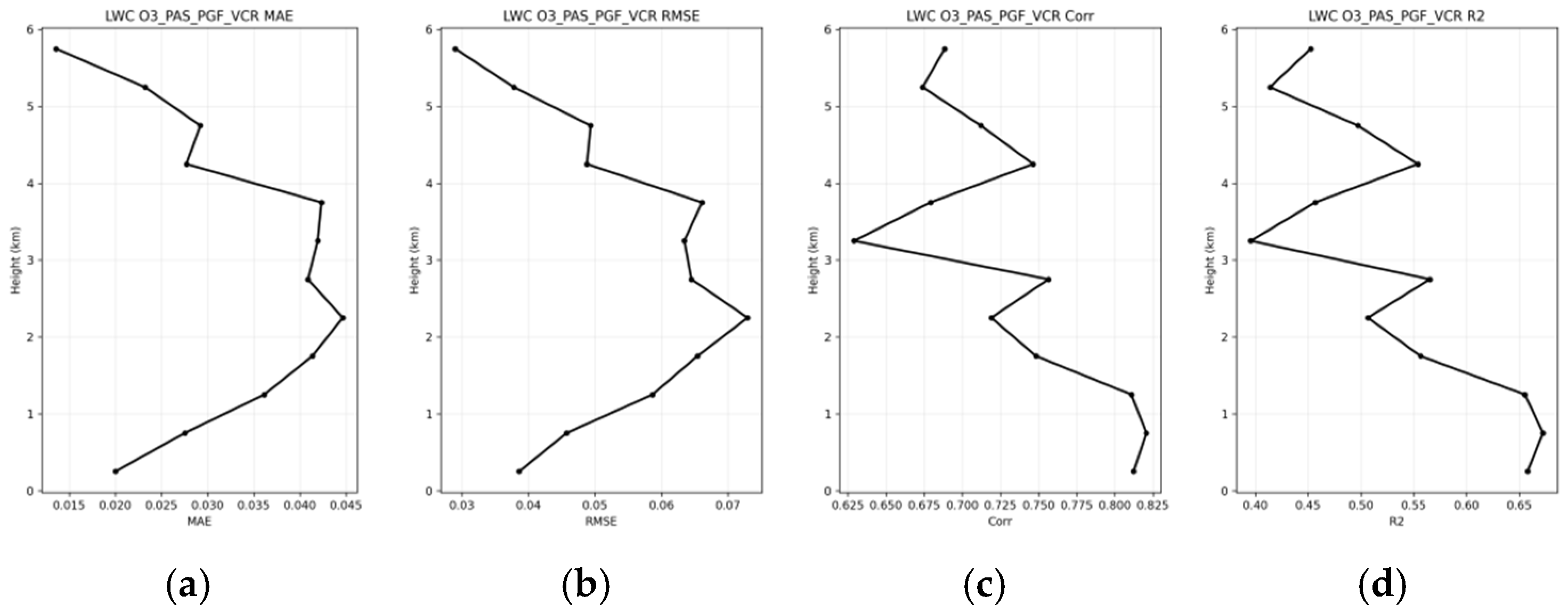
For LWC retrieval, altitude dependence is weaker than for IWC. The best performance occurs in the 0–2 km layer, where the model achieves the highest coefficient of determination and the lowest error levels. Accuracy decreases in the 2–4 km layer despite the largest number of samples, likely due to frequent mixed-phase processes that introduce stronger microphysical variability and reduce the stability of the statistical relationship between radar observations and liquid water content.
Table 6 summarizes the height-dependent performance metrics for LWC retrieval. The results indicate moderate variability across altitude ranges.
Performance improves slightly in the 4–6 km layer R 2 0.543 , suggesting more organized cloud structures above the mixed-phase transition region. The vertical profiles shown in Figure 7 confirm that error metrics remain relatively stable with altitude, while correlation metrics vary moderately, indicating robust model performance across different atmospheric layers.

3.3. Ablation Experiment

To examine the contribution of individual variables and model components, two sets of ablation experiments were conducted: input-variable exclusion analysis and stepwise module ablation analysis.
(1)
Input-variable exclusion analysis
The results for IWC retrieval are summarized in Table 7. Compared with the full predictor configuration, removing temperature causes the largest degradation in model performance, with RMSE increasing from 0.0092 to 0.0182 and R2 decreasing from 0.784 to 0.201. This result indicates that temperature provides a dominant thermodynamic constraint for IWC retrieval. Physically, this is consistent with the strong dependence of ice-phase processes on temperature, including saturation vapor pressure, ice nucleation conditions, and depositional growth. Removing radar reflectivity also leads to substantial performance degradation, with RMSE increasing to 0.0192 and R2 decreasing to 0.244. This suggests that radar reflectivity provides important observational information on hydrometeor scattering and cloud vertical structure.
Excluding relative humidity or height-related information also reduces retrieval performance, although the impact is smaller than that caused by removing temperature or radar reflectivity. The weak performance of the height-only and radar-only configurations further indicates that IWC cannot be reliably retrieved from a single category of predictor. The height-only configuration mainly reflects the climatological vertical background of IWC occurrence, whereas the radar-only configuration captures only radar-observed echo structure without thermodynamic constraints. Therefore, accurate IWC retrieval requires the joint use of radar-observed cloud structure, thermodynamic state, and vertical-context information.
For LWC retrieval, the results summarized in Table 8 show a different sensitivity pattern. Removing radar reflectivity causes the largest degradation among the variable-exclusion experiments, with RMSE increasing from 0.0591 to 0.0883 and R2 decreasing from 0.606 to 0.209. This indicates that radar reflectivity provides important scattering-related and structural information on liquid-cloud vertical organization. However, radar reflectivity should not be interpreted as a direct measurement of LWC. Radar reflectivity is strongly weighted toward larger hydrometeors and depends on higher-order moments of the particle size distribution, whereas LWC is more closely related to hydrometeor mass. Therefore, radar reflectivity alone cannot uniquely determine LWC without thermodynamic and vertical-context information.
Removing temperature, relative humidity, or height-related information also degrades LWC retrieval performance, confirming that liquid-water retrieval depends on multiple sources of information. The similar performance of the height-only and radar-only configurations does not imply that radar reflectivity provides little useful information. Instead, it indicates that each single-source predictor captures only a limited aspect of the retrieval problem. The height-only configuration mainly represents the climatological vertical distribution of LWC, such as the tendency for liquid water to occur more frequently in lower cloud layers. In contrast, the radar-only configuration provides information on cloud echo structure but lacks temperature, humidity, and vertical-position constraints. As a result, both configurations show limited skill and cannot adequately represent the actual LWC variability of a specific profile.
The input-variable ablation results indicate that the retrieval skill of the full framework arises from the complementary use of radar reflectivity, thermodynamic predictors, and height-related information. For IWC retrieval, temperature provides a particularly important thermodynamic constraint, whereas radar reflectivity supplies observational information on hydrometeor scattering and cloud vertical structure. For LWC retrieval, removing radar reflectivity causes the largest degradation among the variable-exclusion experiments, but radar reflectivity remains insufficient when used alone. These results support the use of a multisource and vertically structured predictor space rather than relying on any single predictor group.
(2)
Stepwise module ablation analysis
Module contributions were further evaluated through stepwise ablation experiments, in which the proposed framework was progressively enhanced from the baseline Random Forest model by adding VSE, PAS, and finally PGF + VCR.
For LWC retrieval, the results are summarized in Table 9. The baseline Random Forest model achieves R2 = 0.303. Introducing VSE increases R2 to 0.494, demonstrating that explicit representation of vertical gradients and local profile statistics provides the largest single performance gain. This result indicates that a major limitation of the baseline model lies in its inability to represent vertical structural context when each height level is treated independently.
Adding PAS further increases R2 to 0.507, suggesting that the profile-aware stacking strategy mainly improves generalization by reducing variance through ensemble integration. Although the improvement relative to VSE is smaller, PAS provides a more stable prediction framework across heterogeneous cloud regimes.
The final framework, including PGF and VCR, increases R2 to 0.606 and reduces RMSE to 0.0591, indicating that profile-level structural priors and refinement constraints improve vertical consistency beyond pointwise accuracy alone. These modules, therefore, contribute primarily to the vertical structural coherence of the predicted LWC profiles rather than only to the local regression fit.
The scatter-density distributions in Figure 8 visually confirm these improvements. Compared with the baseline model, the final framework exhibits a tighter concentration around the 1:1 reference line, reduced spread of residuals, and noticeably less prediction dispersion, indicating both improved accuracy and improved stability.
For IWC retrieval, the module-ablation results summarized in Table 10 show a similar but even clearer pattern. The baseline model achieves R2 = 0.412. Adding VSE increases R2 to 0.688, again indicating that explicit encoding of vertical structural information provides the largest contribution to performance improvement. This large gain suggests that IWC retrieval benefits strongly from local vertical gradients and profile context, which are closely linked to the layered structure of ice clouds.
Incorporating PAS further improves R2 to 0.744, showing that ensemble diversity and profile-aware meta-learning improve model robustness. The complete framework, including PGF and VCR, achieves the best performance with R2 = 0.784 and RMSE = 0.0092. This final improvement indicates that the PGF variables and VCR step help suppress nonphysical oscillations and enhance profile-scale coherence in the retrieved IWC fields.
The corresponding scatter-density distributions in Figure 9 show a noticeably tighter alignment with the 1:1 reference line, confirming improved agreement between predicted and observed IWC values. Relative to the baseline model, the final framework reduces both spread and bias in the high-density prediction region, indicating that the added modules improve not only average error statistics but also the structural fidelity of the retrieved profiles.
The ablation experiments demonstrate that the largest performance gain comes from explicit representation of vertical structure through VSE, while PAS improves generalization through ensemble diversity, and PGF + VCR further enhances profile-level structural consistency. Together, these results provide direct empirical support for the hierarchical design of the proposed retrieval framework.

3.4. Boundary-Region Evaluation

To further examine whether the proposed framework improves retrieval performance in structurally complex cloud regions, an additional boundary-region evaluation was conducted. Cloud-boundary samples were defined using radar-derived cloud-base and cloud-top heights. Samples located within three radar range gates, approximately 90 m, from either cloud base or cloud top were classified as near-boundary samples, while the remaining in-cloud samples were classified as cloud-interior samples. The baseline random forest model and the proposed framework were then evaluated separately in these two regions for both IWC and LWC retrieval. The results are summarized in Table 11.
For IWC retrieval, the proposed framework shows a substantial improvement over the baseline RF model in the near-boundary region. The baseline RF model performs poorly near cloud boundaries, with an RMSE of 0.0090 g m−3, a negative R2 of −1.716, and a low correlation coefficient of 0.131. In contrast, the proposed method reduces RMSE to 0.0038 g m−3 and increases R2 and Corr. to 0.524 and 0.729, respectively. This result indicates that the proposed framework is more effective in representing IWC variability near cloud boundaries, where cloud structure and hydrometeor content may change rapidly with height.
In the cloud-interior region, the proposed method also improves IWC retrieval performance, reducing RMSE from 0.0181 to 0.0111 g m−3 and increasing R2 from 0.253 to 0.719. Although improvements are observed in both regions, the near-boundary result is particularly important because it demonstrates that the proposed framework does not only improve vertically averaged statistics, but also enhances retrieval performance in boundary regions that are more challenging for pointwise models.
For LWC retrieval, the proposed method also outperforms the baseline RF model in both near-boundary and cloud-interior regions. Near cloud boundaries, RMSE decreases from 0.0929 to 0.0642 g m−3, while R2 increases from 0.205 to 0.619 and Corr. increases from 0.475 to 0.789. In the cloud-interior region, RMSE decreases from 0.0797 to 0.0590 g m−3, and R2 increases from 0.223 to 0.574. These results suggest that the proposed framework improves the retrieval of liquid water content not only in relatively stable cloud interiors, but also near cloud boundaries where liquid water occurrence and vertical structure can be more variable.

3.5. Cross-Site Evaluation

Additional experiments were conducted using observations from two independent Cloudnet stations, Munich and Jülich, to assess model performance under different atmospheric conditions. In this setup, the model was trained exclusively on the Lindenberg dataset and then directly applied to the Munich and Jülich datasets without retraining or parameter adjustment. The cross-site evaluation results are summarized in Table 12.
For IWC retrieval, the model achieves an RMSE of 0.0573 g m−3, an R2 of 0.680, and a correlation coefficient of 0.824 for the Munich dataset. When applied to the Jülich dataset, the RMSE increases to 0.0880 g m−3, while the R2 decreases to 0.444 and the correlation coefficient to 0.670.
For LWC retrieval, the Munich dataset yields an RMSE of 0.3882 g m−3, an R2 of 0.376, and a correlation coefficient of 0.640. In contrast, the Jülich dataset shows improved performance, with an RMSE of 0.2420 g m−3, an R2 of 0.547, and a correlation coefficient of 0.748. These results indicate that cross-site performance degradation is reflected not only in increased prediction errors but also in reduced explained variance and weakened statistical consistency between predicted and reference values. The cross-site results demonstrate that the proposed framework exhibits limited generalization capability across independent observational environments, with the degradation being more pronounced for LWC retrieval. The substantial increase in RMSE and the reduction in correlation, particularly for the Munich dataset, suggest that the learned feature–target relationships are sensitive to site-specific atmospheric conditions. This implies that a model trained on a single site cannot fully capture the variability associated with different local cloud regimes and thermodynamic environments. This limitation is likely associated with distribution shifts in both thermodynamic conditions and radar–microphysics relationships across sites. This highlights the necessity of incorporating multi-site training data or domain adaptation strategies to improve model transferability across heterogeneous atmospheric conditions.

4. Discussion

The improvement achieved by the proposed framework is mainly associated with its explicit representation of vertical structure. In conventional pointwise models, each height level is treated as an independent sample, and vertical dependencies are only implicitly represented through shared predictors. This assumption is limited for cloud-water retrieval because cloud microphysical properties often vary coherently along the vertical dimension and may change rapidly near cloud boundaries. By introducing gradient-based descriptors and local contextual features, the proposed framework provides the model with additional information on vertical transitions that cannot be fully represented by single-level predictors alone. This explains why the inclusion of VSE produces the largest performance gain in the stepwise ablation experiments.
The importance of vertical structure is further supported by the boundary-region evaluation. Near radar-derived cloud boundaries, the proposed framework reduced IWC RMSE from 0.0090 to 0.0038 g m−3 and increased R2 from −1.716 to 0.524. For LWC, the near-boundary RMSE decreased from 0.0929 to 0.0642 g m−3, while R2 increased from 0.205 to 0.619. These results indicate that the proposed vertical-context and cloud-geometry representations are particularly beneficial in regions where hydrometeor content and radar reflectivity may vary sharply over short vertical distances. The strong degradation of the baseline RF model near cloud boundaries also suggests that neglecting vertical context is an important source of error in pointwise retrieval, rather than merely a consequence of insufficient model complexity.
The different sensitivities of IWC and LWC retrievals reflect the distinct physical controls governing ice- and liquid-phase clouds. IWC retrieval is strongly influenced by temperature because ice nucleation, depositional growth, saturation conditions, and particle habit evolution are closely linked to thermodynamic state. This is consistent with the input-variable ablation results, where removing temperature produces the largest degradation in IWC performance.
In contrast, LWC retrieval shows greater sensitivity to the inclusion of radar reflectivity, indicating that radar observations provide useful information on liquid-cloud echo structure. However, radar reflectivity should not be interpreted as a direct measurement of LWC. Reflectivity is strongly weighted toward larger hydrometeors and depends on higher-order moments of the particle size distribution, whereas LWC is more closely related to hydrometeor mass. The relatively stronger usefulness of radar reflectivity for LWC retrieval in the present experiments is therefore better interpreted from the perspective of scattering uncertainty: liquid droplets are more nearly spherical and have a stronger dielectric response at 35 GHz, whereas ice-particle retrievals are additionally affected by particle habit, density, orientation, and temperature-dependent microphysical processes. Therefore, the role of radar reflectivity in LWC retrieval should be understood as providing structural and scattering-related information that becomes useful only when combined with thermodynamic and vertical-context predictors.
The cross-site evaluation highlights the limited transferability of the current single-site training strategy. When the model trained at Lindenberg was applied directly to Munich and Jülich, retrieval performance degraded, especially for LWC. This suggests that the statistical relationships learned at one site are not fully invariant across different observational environments. Such degradation is likely related to site-specific differences in boundary-layer structure, aerosol conditions, shallow-cloud evolution, cloud-boundary characteristics, and mixed-phase occurrence, all of which can modify the relationship between radar reflectivity, thermodynamic profiles, and Cloudnet-derived hydrometeor products. The relatively better transferability observed for IWC may reflect the stronger dependence of ice-phase processes on larger-scale thermodynamic structure, whereas LWC is more strongly affected by local boundary-layer and shallow-cloud variability. These results indicate that multi-site training, site-aware calibration, or domain adaptation may be necessary for robust application across heterogeneous cloud regimes.
Several limitations should also be noted. First, the framework remains fully data-driven and does not explicitly enforce physical constraints such as mass conservation, phase consistency, or microphysical closure. Although the vertical refinement step reduces small-scale oscillations, it cannot guarantee physically consistent profiles under all cloud conditions, particularly in mixed-phase clouds where microphysical processes are highly nonlinear. Second, the boundary-region evaluation is based on radar-derived cloud-base and cloud-top definitions. It therefore provides direct evidence for improved retrieval near cloud boundaries, but it should not be interpreted as a complete validation of all phase-transition processes. Third, Cloudnet LWC and IWC products are used as reference targets, but they are themselves retrieval-based estimates and contain uncertainties related to instrument sensitivity, retrieval assumptions, and microphysical parameterisations. The reported metrics therefore quantify agreement with Cloudnet reference products rather than absolute physical accuracy. Future work should incorporate stronger physical constraints into the learning process, extend the training dataset to multiple sites and cloud regimes, and investigate domain-adaptation strategies to improve generalization under changing observational conditions.

5. Conclusions

This study formulated cloud liquid water content (LWC) and ice water content (IWC) retrieval as a vertically structured learning problem by integrating Cloudnet hydrometeor products with cloud radar reflectivity and microwave-radiometer-derived thermodynamic profiles. The proposed framework explicitly incorporated vertical-structure-enhanced features, profile-aware stacking, cloud-geometry information, and vertical consistency refinement to improve both pointwise retrieval accuracy and profile-level coherence.
Using year-round observations from the Lindenberg Cloudnet site, the proposed framework consistently outperformed conventional pointwise and general-purpose machine-learning models. For IWC retrieval, RMSE decreased from 0.0152 to 0.0092 g m−3, while R2 increased from 0.412 to 0.784. For LWC retrieval, RMSE decreased from 0.0786 to 0.0591 g m−3, while R2 increased from 0.303 to 0.606. Ablation experiments further showed that vertical-structure-enhanced features made the largest contribution to the overall improvement.
Boundary-region evaluation further confirmed that the proposed framework improves retrieval performance in structurally complex parts of cloud profiles, particularly near radar-derived cloud boundaries where hydrometeor content can change rapidly with height.
The two retrieval tasks showed different sensitivities to input variables. IWC retrieval was strongly constrained by thermodynamic conditions, particularly temperature, reflecting the role of temperature-dependent ice-phase processes. In contrast, LWC retrieval showed stronger sensitivity to the inclusion of radar reflectivity, which provides important information on liquid-cloud echo structure. However, radar reflectivity alone was insufficient for reliable LWC retrieval, highlighting the need to combine radar-observed cloud structure with thermodynamic and vertical-context information.
Cross-site evaluation revealed that the learned relationships were sensitive to site-specific atmospheric conditions. Models trained at Lindenberg showed degraded performance when directly applied to Munich and Jülich, especially for LWC retrieval. This indicates that single-site training is insufficient to fully represent variations in boundary-layer structure, shallow-cloud processes, and local cloud regimes across different observational environments. Future applications should therefore consider multi-site training, site-aware calibration, or domain-adaptation strategies to improve robustness and transferability.
These findings suggest that cloud-water profile retrieval should not be treated only as an independent pointwise regression problem, but also as a vertically organized profile-retrieval task. By incorporating vertical context, cloud-geometry information, and profile-level refinement, the proposed framework provides a practical data-driven approach for improving LWC and IWC profile retrieval from ground-based remote-sensing observations. This perspective may also provide a useful basis for other profile-based atmospheric retrieval tasks, such as thermodynamic profiling, aerosol retrieval, and data-assimilation-oriented cloud analysis.


Author Contributions

Conceptualization, Z.P., Y.B. and H.W.; methodology, Z.P. and H.W.; software, Z.P.; validation, Z.P.; formal analysis, Z.P.; investigation, Z.P.; data curation, Z.P.; writing—original draft preparation, Z.P.; writing—review and editing, Z.P., Y.B., H.W. and H.L.; visualization, Z.P.; supervision, H.W., Y.B. and H.L.; project administration, H.W.; funding acquisition, Y.B., F.P. and W.T. All authors have read and agreed to the published version of the manuscript.

Funding

This research was funded by Fengyun Application Pioneering Project (FY-APP), Guangxi Key Research and Development Program (Guangxi Science and Technology Program under Grant, AB25069126) and The Natural Science Foundation of China (U2242212).

Data Availability Statement

The data supporting the findings of this study are available from the corresponding author upon reasonable request. The datasets used and/or analyzed during the current study are not publicly available due to project-related restrictions.

Acknowledgments

The authors gratefully acknowledge Nanjing University of Information and University of Reading Science and Technology for providing academic support and research facilities. The financial support from the China Scholarship Council (CSC) is also sincerely appreciated. During the preparation of this manuscript, the authors used ChatGPT-5.5 by OpenAI for language polishing. The authors have carefully reviewed and revised the content and take full responsibility for the final manuscript.

Conflicts of Interest

The authors declare no conflicts of interest.

Abbreviations

The following abbreviations are used in this manuscript:
LWCCloud Liquid Water Content
IWCIce Water Content
MWRMicrowave Radiometer
ZeEquivalent Radar Reflectivity Factor
VSEVertical-Structure-Enhanced Features
PASProfile-Aware Stacking
PGFProfile Grouping Framework
VCRVertical Consistency Refinement
RFRandom Forest
MLPMultilayer Perceptron
LSTMLong Short-Term Memory
HGBHistogram-based Gradient Boosting
MLRMultiple Linear Regression
RMSERoot Mean Square Error
MAEMean Absolute Error
Corr.Correlation Coefficient
R2Coefficient of Determination
ARMAtmospheric Radiation Measurement
MIRA-35METEK 35 GHz Ka-band cloud radar

Appendix A. Height-Dependent Distributions of LWC and IWC Samples

The processed Cloudnet-derived hydrometeor samples show clear altitude-dependent distribution characteristics. To document these characteristics, the distributions of ice water content (IWC) and liquid water content (LWC) were examined separately within the altitude intervals used for dataset characterization. IWC samples were grouped into 0–3 km, 3–6 km, and 6–9 km layers, while LWC samples were grouped into 0–2 km, 2–4 km, and 4–6 km layers. These altitude intervals were used only to describe the dataset and to support height-dependent analysis. They were not used to train separate retrieval models.
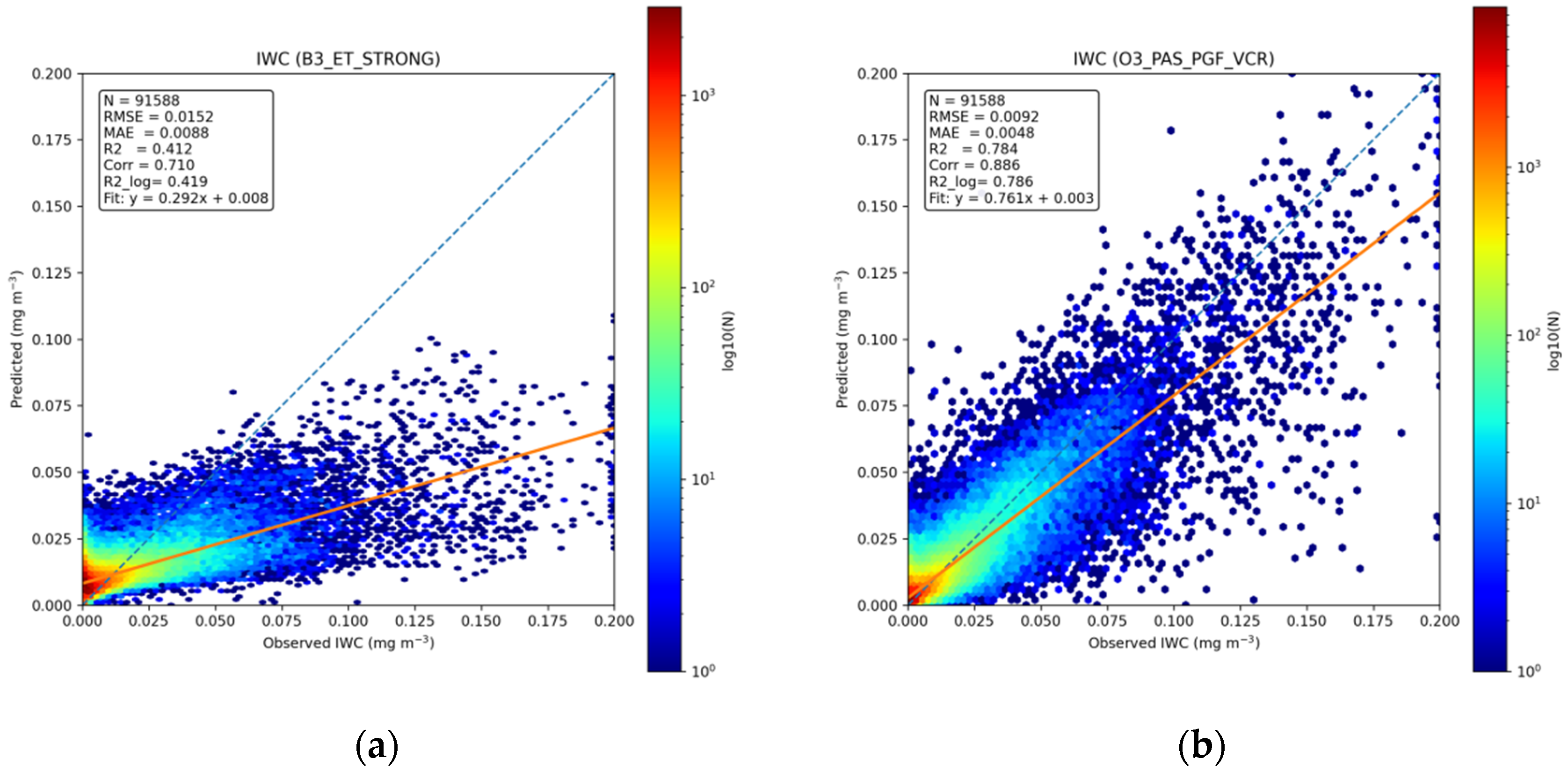
Figure A1 shows the IWC distributions in the three altitude intervals. In the 0–3 km layer, the distribution contains a large number of very small IWC values, with a median of 2.45 × 10⁻⁶ kg m−3 and a mean of 5.96 × 10⁻⁵ kg m−3. This indicates that low-level IWC samples are dominated by weak ice signals, although relatively larger values also occur. In the 3–6 km layer, the median increases to 1.09 × 10⁻⁵ kg m−3, while the mean remains similar at 5.73 × 10⁻⁵ kg m−3, suggesting a stronger and more frequent occurrence of ice-phase hydrometeors in the middle troposphere. In the 6–9 km layer, the distribution becomes more concentrated around lower-to-moderate IWC values, with a mean of 1.90 × 10⁻⁵ kg m−3 and a median of 6.53 × 10⁻⁶ kg m−3. These patterns confirm that IWC exhibits substantial vertical heterogeneity, supporting the need to include height and vertical-structure information in the retrieval framework.
Figure A1. Height-dependent distributions of ice water content (IWC) samples in the processed dataset. Panels show the distributions for (a) 0–3 km, (b) 3–6 km, and (c) 6–9 km. Dashed and dash-dotted vertical lines indicate the median and mean values, respectively. The altitude coverage of valid IWC records above 9 km is discussed in Section 2.4.3.
Remotesensing 18 02177 g0a1
Figure A2 shows the corresponding LWC distributions. LWC is mainly concentrated in the lower and middle troposphere, with the largest sample size occurring in the 0–2 km layer. In this layer, the mean and median LWC values are 2.08 × 10⁻⁴ kg m−3 and 8.41 × 10⁻⁵ kg m−3, respectively. In the 2–4 km layer, the distribution remains broadly similar, with a mean of 1.96 × 10⁻⁴ kg m−3 and a median of 7.80 × 10⁻⁵ kg m−3. In contrast, the 4–6 km layer contains far fewer samples and lower LWC values, with the mean decreasing to 6.02 × 10⁻⁵ kg m−3 and the median decreasing to 1.88 × 10⁻⁵ kg m−3. This confirms that liquid water is more concentrated at lower altitudes, while high-altitude LWC occurrence is less frequent and generally weaker.
Figure A2. Height-dependent distributions of liquid water content (LWC) samples in the processed dataset. Panels show the distributions for (a) 0–2 km, (b) 2–4 km, and (c) 4–6 km. Dashed and dash-dotted vertical lines indicate the median and mean values, respectively.
Remotesensing 18 02177 g0a2
These distributions provide additional evidence that LWC and IWC have distinct vertical occurrence patterns and magnitude ranges. IWC shows stronger vertical variation across the lower, middle, and upper layers, whereas LWC is more concentrated below 4 km and decreases markedly in both sample size and magnitude in the 4–6 km layer. This height-dependent behaviour supports the use of a unified retrieval framework that includes explicit height information, local vertical gradients, profile-relative descriptors, and cloud-geometry variables, rather than treating the retrieval targets as vertically homogeneous variables.

References

  1. Stephens, G.L. Cloud feedbacks in the climate system: A critical review. J. Clim. 2005, 18, 237–273. [Google Scholar] [CrossRef]
  2. Shupe, M.D.; Intrieri, J.M. Cloud radiative forcing of the Arctic surface: The influence of cloud properties, surface albedo, and solar zenith angle. J. Clim. 2004, 17, 616–628. [Google Scholar] [CrossRef]
  3. Matus, A.V.; L’Ecuyer, T.S. The role of cloud phase in Earth’s radiation budget. J. Geophys. Res. Atmos. 2017, 122, 2559–2578. [Google Scholar] [CrossRef]
  4. Morrison, H.; de Boer, G.; Feingold, G.; Harrington, J.; Shupe, M.D.; Sulia, K. Resilience of persistent Arctic mixed-phase clouds. Nat. Geosci. 2012, 5, 11–17. [Google Scholar] [CrossRef]
  5. Mülmenstädt, J.; Sourdeval, O.; Delanoë, J.; Quaas, J. Frequency of occurrence of rain from liquid-, mixed-, and ice-phase clouds derived from A-Train satellite retrievals. Geophys. Res. Lett. 2015, 42, 6502–6509. [Google Scholar] [CrossRef]
  6. Choi, Y.-S.; Ho, C.-H.; Park, C.-E.; Storelvmo, T.; Tan, I. Influence of cloud phase composition on climate feedbacks. J. Geophys. Res. Atmos. 2014, 119, 3687–3700. [Google Scholar] [CrossRef]
  7. Korolev, A.; McFarquhar, G.; Field, P.R.; Franklin, C.; Lawson, P.; Wang, Z.; Williams, E.; Abel, S.J.; Axisa, D.; Borrmann, S.; et al. Mixed-phase clouds: Progress and challenges. Meteorol. Monogr. 2017, 58, 5.1–5.50. [Google Scholar] [CrossRef]
  8. Radenz, M.; Bühl, J.; Seifert, P.; Baars, H.; Engelmann, R.; Barja González, B.; Mamouri, R.E.; Zamorano, F.; Ansmann, A. Hemispheric contrasts in ice formation in stratiform mixed-phase clouds: Disentangling the role of aerosol and dynamics with ground-based remote sensing. Atmos. Chem. Phys. 2021, 21, 17969–17994. [Google Scholar] [CrossRef]
  9. Tan, I.; Storelvmo, T.; Zelinka, M.D. Observational constraints on mixed-phase clouds imply higher climate sensitivity. Science 2016, 352, 224–227. [Google Scholar] [CrossRef] [PubMed]
  10. Cesana, G.V.; Ackerman, A.S.; Fridlind, A.M.; Silber, I.; Del Genio, A.D.; Zelinka, M.D.; Chepfer, H.; Khadir, T.; Roehrig, R. Observational constraint on a feedback from supercooled clouds reduces projected warming uncertainty. Commun. Earth Environ. 2024, 5, 181. [Google Scholar] [CrossRef]
  11. Pithan, F.; Medeiros, B.; Mauritsen, T. Mixed-phase clouds cause climate model biases in Arctic wintertime temperature inversions. Clim. Dyn. 2014, 43, 289–303. [Google Scholar] [CrossRef]
  12. Aubry, C.; Delanoë, J.; Groß, S.; Ewald, F.; Tridon, F.; Jourdan, O.; Mioche, G. Lidar–radar synergistic method to retrieve ice, supercooled water and mixed-phase cloud properties. Atmos. Meas. Tech. 2024, 17, 3863–3881. [Google Scholar] [CrossRef]
  13. Riihimaki, L.D.; Comstock, J.M.; Anderson, K.K.; Holmes, A.; Luke, E. A path towards uncertainty assignment in an operational cloud-phase algorithm from ARM vertically pointing active sensors. Adv. Stat. Climatol. Meteorol. Oceanogr. 2016, 2, 49–62. [Google Scholar] [CrossRef]
  14. Shupe, M.D. A ground-based multisensor cloud phase classifier. Geophys. Res. Lett. 2007, 34, L22809. [Google Scholar] [CrossRef]
  15. Illingworth, A.J.; Hogan, R.J.; O’Connor, E.J.; Bouniol, D.; Brooks, M.E.; Delanoë, J.; Donovan, D.P.; Eastment, J.D.; Gaussiat, N.; Goddard, J.W.F.; et al. Cloudnet: Continuous evaluation of cloud profiles in seven operational models using ground-based observations. Bull. Am. Meteorol. Soc. 2007, 88, 883–898. [Google Scholar] [CrossRef]
  16. Shupe, M.D.; Turner, D.D.; Zwink, A.; Thieman, M.M.; Mlawer, E.J.; Shippert, T. Deriving Arctic cloud microphysics at Barrow, Alaska: Algorithms, results, and radiative closure. J. Appl. Meteorol. Climatol. 2015, 54, 1675–1689. [Google Scholar] [CrossRef]
  17. Shupe, M.D.; Comstock, J.M.; Turner, D.D.; Mace, G.G. Cloud property retrievals in the ARM Program. Meteorol. Monogr. 2016, 57, 19.1–19.20. [Google Scholar] [CrossRef]
  18. Tukiainen, S.; O’Connor, E.; Korpinen, A. CloudnetPy: A Python package for processing cloud remote sensing data. J. Open Source Softw. 2020, 5, 2123. [Google Scholar] [CrossRef]
  19. Griesche, H.J.; Seifert, P.; Engelmann, R.; Radenz, M.; Hofer, J.; Althausen, D.; Walbröl, A.; Barrientos-Velasco, C.; Baars, H.; Dahlke, S.; et al. Cloud micro- and macrophysical properties from ground-based remote sensing during the MOSAiC drift experiment. Sci. Data 2024, 11, 505. [Google Scholar] [CrossRef] [PubMed]
  20. Delanoë, J.; Hogan, R.J. A variational scheme for retrieving ice cloud properties from combined radar, lidar, and infrared radiometer. J. Geophys. Res. Atmos. 2008, 113, D07204. [Google Scholar] [CrossRef]
  21. Mason, S.L.; Hogan, R.J.; Bozzo, A.; Pounder, N.L. A unified synergistic retrieval of clouds, aerosols, and precipitation from EarthCARE: The ACM-CAP product. Atmos. Meas. Tech. 2023, 16, 3459–3486. [Google Scholar] [CrossRef]
  22. Kalesse-Los, H.; Schimmel, W.; Luke, E.; Seifert, P. Evaluating cloud liquid detection against Cloudnet using cloud radar Doppler spectra in a pre-trained artificial neural network. Atmos. Meas. Tech. 2022, 15, 279–295. [Google Scholar] [CrossRef]
  23. Silber, I.; Verlinde, J.; Wen, G.; Eloranta, E.W. Can embedded liquid cloud layer volumes be classified in polar clouds using a single-frequency zenith-pointing radar? IEEE Geosci. Remote Sens. Lett. 2020, 17, 222–226. [Google Scholar] [CrossRef]
  24. Luke, E.P.; Kollias, P.; Shupe, M.D. Detection of supercooled liquid in mixed-phase clouds using radar Doppler spectra. J. Geophys. Res. Atmos. 2010, 115, D19201. [Google Scholar] [CrossRef]
  25. Kalogeras, P.; Battaglia, A.; Kollias, P. Supercooled liquid water detection capabilities from Ka-band Doppler profiling radars: Moment-based algorithm formulation and assessment. Remote Sens. 2021, 13, 2891. [Google Scholar] [CrossRef]
  26. Kalesse, H.; de Boer, G.; Solomon, A.; Oue, M.; Ahlgrimm, M.; Zhang, D.; Shupe, M.D.; Luke, E.; Protat, A. Understanding rapid changes in phase partitioning between cloud liquid and ice in stratiform mixed-phase clouds: An Arctic case study. Mon. Weather Rev. 2016, 144, 4805–4826. [Google Scholar] [CrossRef]
  27. Cazenave, Q.; Ceccaldi, M.; Delanoë, J.; Pelon, J.; Groß, S.; Heymsfield, A. Evolution of DARDAR-CLOUD ice cloud retrievals: New parameters and impacts on the retrieved microphysical properties. Atmos. Meas. Tech. 2019, 12, 2819–2835. [Google Scholar] [CrossRef]
  28. Maskey, M. Advancing AI for Earth science: A data systems perspective. In Proceedings of the ESA EO Phi-Week, Virtual Event, 28 September–2 October 2020. [Google Scholar]
  29. Vogl, T.; Maahn, M.; Kneifel, S.; Schimmel, W.; Moisseev, D.; Kalesse-Los, H. Using artificial neural networks to predict riming from Doppler cloud radar observations. Atmos. Meas. Tech. 2022, 15, 365–381. [Google Scholar] [CrossRef]
  30. Kalesse, H.; Vogl, T.; Paduraru, C.; Luke, E. Development and validation of a supervised machine learning radar Doppler spectra peak-finding algorithm. Atmos. Meas. Tech. 2019, 12, 4591–4617. [Google Scholar] [CrossRef]
  31. Radenz, M.; Bühl, J.; Seifert, P.; Griesche, H.; Engelmann, R. peakTree: A framework for structure-preserving radar Doppler spectra analysis. Atmos. Meas. Tech. 2019, 12, 4813–4828. [Google Scholar] [CrossRef]
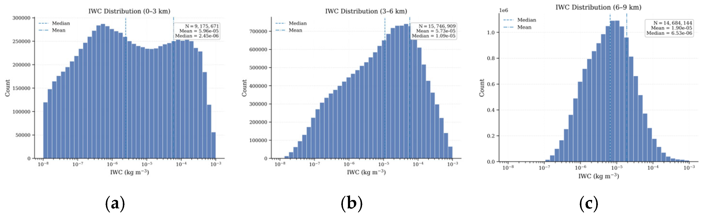
  32. Schimmel, W.; Kalesse-Los, H.; Maahn, M.; Vogl, T.; Foth, A.; Garfias, P.S.; Seifert, P. Identifying cloud droplets beyond lidar attenuation from vertically pointing cloud radar observations using artificial neural networks. Atmos. Meas. Tech. 2022, 15, 5343–5366. [Google Scholar] [CrossRef]
  33. Goldberger, L.; Levin, M.; Harris, C.; Geiss, A.; Shupe, M.D.; Zhang, D. Classifying thermodynamic cloud phase using machine learning models. Atmos. Meas. Tech. 2025, 18, 5393–5414. [Google Scholar] [CrossRef]
  34. Cadeddu, M.P.; Turner, D.D.; Liljegren, J.C. A neural network for real-time retrievals of PWV and LWP from Arctic millimeter-wave ground-based observations. IEEE Trans. Geosci. Remote Sens. 2009, 47, 1887–1900. [Google Scholar]
  35. Strandgren, J.; Bugliaro, L.; Sehnke, F.; Schröder, L. Cirrus cloud retrieval with MSG/SEVIRI using artificial neural networks. Atmos. Meas. Tech. 2017, 10, 3547–3573. [Google Scholar] [CrossRef]
  36. Andersen, H.; Cermak, J.; Fuchs, J.; Knutti, R.; Lohmann, U. Understanding the drivers of marine liquid-water cloud occurrence and properties with global observations using neural networks. Atmos. Chem. Phys. 2017, 17, 9535–9546. [Google Scholar] [CrossRef]
  37. Yan, J.; Oue, M.; Kollias, P.; Luke, E.; Yang, F. A radar view of ice microphysics and turbulence in Arctic cloud systems. Atmos. Chem. Phys. 2025, 25, 16479–16490. [Google Scholar] [CrossRef]
  38. Liao, L.; Meneghini, R.; Tokay, A.; Bliven, L.F. Retrieval of snow properties for Ku- and Ka-band dual-frequency radar. J. Appl. Meteorol. Climatol. 2016, 55, 1845–1858. [Google Scholar] [CrossRef] [PubMed]
  39. Löhnert, U.; Maier, O. Operational profiling of temperature using ground-based microwave radiometry at Payerne: Prospects and challenges. Atmos. Meas. Tech. 2012, 5, 1121–1134. [Google Scholar] [CrossRef]
  40. Foth, A.; Lochmann, M.; Saavedra Garfias, P.; Kalesse-Los, H. Determination of low-level temperature profiles from microwave radiometer observations during rain. Atmos. Meas. Tech. 2024, 17, 7169–7181. [Google Scholar] [CrossRef]
  41. Bianco, L.; Adler, B.; Bariteau, L.; Djalalova, I.V.; Myers, T.; Pezoa, S.; Turner, D.D.; Wilczak, J.M. Sensitivity of thermodynamic profiles retrieved from ground-based microwave and infrared observations to additional input data from active remote sensing instruments and numerical weather prediction models. Atmos. Meas. Tech. 2024, 17, 3933–3948. [Google Scholar] [CrossRef]
  42. Reale, T.; Sun, B.; Tilley, F.H.; Pettey, M. The NOAA Products Validation System (NPROVS). J. Atmos. Ocean. Technol. 2012, 29, 629–645. [Google Scholar] [CrossRef]
  43. Breiman, L. Random forests. Mach. Learn. 2001, 45, 5–32. [Google Scholar] [CrossRef]
  44. Kannemadugu, H.B.S.; Verma, M.; Dutta, D.; Johnson, L.R.; Rao, S.; Seshasai, M.V.R. Comparison of temperature and humidity profiles retrieved from INSAT-3DR sounder with high resolution radiosonde measurements. AIMS Geosci. 2021, 7, 180–193. [Google Scholar] [CrossRef]
  45. Sun, B.; Reale, A.; Seidel, D.J.; Hunt, D.C. Comparing radiosonde and COSMIC atmospheric profile data to quantify differences among radiosonde types and the effects of imperfect collocation on comparison statistics. J. Geophys. Res. Atmos. 2010, 115, D23104. [Google Scholar] [CrossRef]
  46. Amell, A.; Eriksson, P.; Pfreundschuh, S. Ice water path retrievals from Meteosat-9 using quantile regression neural networks. Atmos. Meas. Tech. 2022, 15, 5701–5717. [Google Scholar] [CrossRef]
  47. Malmgren-Hansen, D.; Laparra, V.; Nielsen, A.A.; Camps-Valls, G. Statistical retrieval of atmospheric profiles with deep convolutional neural networks. ISPRS J. Photogramm. Remote Sens. 2019, 158, 231–240. [Google Scholar] [CrossRef]
  48. Ridolfi, M.; Sgheri, L. A self-adapting and altitude-dependent regularization method for atmospheric profile retrievals. Atmos. Chem. Phys. 2009, 9, 1883–1897. [Google Scholar] [CrossRef]
  49. Che, Y.; Ma, S.; Xing, F.; Li, S.; Dai, Y. An improvement of the retrieval of temperature and relative humidity profiles from a combination of active and passive remote sensing. Meteorol. Atmos. Phys. 2019, 131, 681–695. [Google Scholar] [CrossRef]
  50. Luo, Y.; Wu, H.; Gu, T.; Wang, Z.; Yue, H.; Wu, G.; Zhu, L.; Pu, D.; Tang, P.; Jiang, M. Machine learning model-based retrieval of temperature and relative humidity profiles measured by microwave radiometer. Remote Sens. 2023, 15, 3838. [Google Scholar] [CrossRef]
Figure 1. Workflow of the proposed vertically structured machine-learning retrieval framework for cloud liquid water content (LWC) and ice water content (IWC) profiles. Cloud radar reflectivity (Ze; METEK MIRA-35, METEK Meteorologische Messtechnik GmbH, Elmshorn, Germany) and microwave radiometer thermodynamic profiles (T, RH; HATPRO-G5, Radiometer Physics GmbH, Meckenheim, Germany) are first corrected using radiosonde observations to reduce thermodynamic biases. The multisource observations are then collocated in time and height (Δt ≤ 60 s, Δh ≤ 30 m) and subjected to quality control. The processed dataset is used to train a random-forest-based retrieval framework incorporating vertical-structure-enhanced features (VSE), a profile-aware stacking ensemble (PAS), a profile grouping framework based on cloud geometry (PGF), and vertical consistency refinement (VCR). Retrieval performance is evaluated using RMSE, MAE, R2, and correlation.
Remotesensing 18 02177 g001
Figure 2. Schematic illustration of the thermodynamic bias-correction procedure for microwave-radiometer-derived profiles. Microwave-radiometer temperature and relative humidity profiles are first matched with radiosonde observations in time and height to construct paired samples. The MWR–radiosonde differences are then decomposed into a height-dependent systematic bias component and a residual component. The height-dependent bias correction removes the mean vertical bias, while the residual learning step further refines the corrected profiles. The corrected temperature and relative humidity profiles are subsequently used as thermodynamic predictors in the LWC/IWC retrieval framework.
Remotesensing 18 02177 g002
Figure 3. Mean-profile comparison of microwave-radiometer-derived thermodynamic variables before and after correction. Panels (a,b) show relative humidity before and after correction, respectively, while panels (c,d) show temperature before and after correction, respectively. Microwave-radiometer-derived profiles are shown as continuous curves, and radiosonde reference profiles are shown with discrete markers at the matched vertical levels. The comparison indicates that the correction reduces height-dependent deviations between the microwave-radiometer-derived and radiosonde-observed thermodynamic profiles.
Remotesensing 18 02177 g003
Figure 4. Scatter-density comparison between microwave-radiometer-derived and radiosonde-observed thermodynamic variables before and after correction. Panels (a,b) show relative humidity before and after correction, respectively, while panels (c,d) show temperature before and after correction, respectively. The red solid line denotes the 1:1 reference line, and the black dashed line denotes the fitted regression line. After correction, the samples become more concentrated around the 1:1 reference line, indicating improved statistical consistency between the microwave-radiometer-derived and radiosonde-observed thermodynamic profiles.
Remotesensing 18 02177 g004
Figure 5. Conceptual comparison between the baseline and the proposed vertically structured LWC/IWC retrieval framework. The proposed framework incorporates vertical-structure-enhanced features, profile-aware stacking, profile-geometry information, and vertical consistency refinement. The arrows in the evaluation section indicate improved performance, with lower RMSE and MAE and higher R2 and correlation.
Remotesensing 18 02177 g005
Figure 6. Vertical profiles of performance metrics for IWC retrieval using the proposed method. Panels show the height-dependent variations of (a) MAE, (b) RMSE, (c) Corr, and (d) R2.
Remotesensing 18 02177 g006
Figure 7. Vertical profiles of performance metrics for LWC retrieval using the proposed method. Panels show the height-dependent variations of (a) MAE, (b) RMSE, (c) Corr, and (d) R2.
Remotesensing 18 02177 g007
Figure 8. Scatter density distributions of predicted versus observed LWC for (a) Baseline RF and (b) the final proposed configuration. Color shading represents the logarithmic density of samples. The blue dashed line denotes the 1:1 reference line, and the orange line denotes the fitted regression line.
Remotesensing 18 02177 g008
Figure 9. Scatter density distributions of predicted versus observed IWC for (a) Baseline RF and (b) the final proposed configuration. Color shading represents the logarithmic density of samples. The blue dashed line denotes the 1:1 reference line, and the orange line denotes the fitted trend line.
Remotesensing 18 02177 g009
Table 1. Statistical comparison between Cloudnet MWR and radiosonde observations before and after bias correction.
VariableStageNCorr.RMSEMAE
Temperature (K)Before correction371,1370.984.803.58
Temperature (K)After correction371,1370.990.720.55
Relative humidity (%)Before correction327,1570.6621.9816.83
Relative humidity (%)After correction327,1570.958.696.55
Table 2. Hyperparameter configurations of baseline machine learning models used in this study.
ModelKey HyperparametersConfiguration
Linear RegressionRegularizationNone
MLPHidden layers3
Hidden units128–64–32
ActivationReLU
OptimizerAdam
Learning rate0.001
Batch size256
Epochs100
LSTMNumber of layers2
Hidden units64
Dropout0.2
OptimizerAdam
Learning rate0.001
Random ForestNumber of trees300
Maximum depth20
Minimum samples per leaf5
Feature samplingsqrt
Histogram-based Gradient BoostingLearning rate0.05
Maximum depth10
Number of iterations300
L2 regularization1.0
Extra TreesNumber of trees300
Maximum depth20
Minimum samples per leaf5
Feature samplingsqrt
Table 3. Performance comparison of different machine learning models for IWC retrieval over the full-year dataset.
ModelMAE (g m−3)RMSE (g m−3)R2Corr.
Proposed Method0.00480.00920.7840.886
MLR (Linear)0.01340.0209−0.1050.074
MLP0.01100.01920.0600.254
LSTM0.01290.01900.0790.327
Random Forest (Baseline)0.00880.01520.4120.710
Extra Trees0.00880.01690.2680.628
HGB0.00940.01750.3360.643
Table 4. Performance comparison of different machine learning models for LWC retrieval over the full-year dataset.
ModelMAE (g m−3)RMSE (g m−3)R2Corr.
Proposed Method0.03530.05910.6060.780
MLR (Linear)0.06230.1012−0.1480.221
MLP0.08610.37320.1490.404
LSTM0.05320.08500.1630.440
Random Forest (Baseline)0.05220.07860.3030.566
Extra Trees0.05910.0981−0.1410.385
HGB0.05530.09120.0480.418
Table 5. Height-dependent performance metrics of the proposed method for IWC retrieval.
Height Range (km)MAE (g m−3)RMSE (g m−3)R2Corr.
0–30.00110.00430.1820.471
3–60.00720.01310.7630.875
6–90.00420.00700.8020.895
Table 6. Height-dependent performance metrics of the proposed method for LWC retrieval.
Height Range (km)MAE (g m−3)RMSE (g m−3)R2Corr.
0–20.03630.05820.6260.792
2–40.04300.06920.5140.722
4–60.04610.06600.5430.737
Table 7. Feature contribution analysis for IWC retrieval based on input-variable exclusion.
FeaturesMAE (g m−3)RMSE (g m−3)R2Corr.
All Features0.00480.00920.7840.886
Without Temperature0.01050.01820.2010.465
Without Relative Humidity0.00910.01620.3700.617
Without Height0.00920.01650.3470.595
Without Radar Reflectivity0.00950.01920.2440.472
Only Height0.01160.01970.0660.271
Only Radar Reflectivity0.01210.02120.0430.223
Table 8. Feature contribution analysis for LWC retrieval based on input-variable exclusion.
FeaturesMAE (g m−3)RMSE (g m−3)R2Corr.
All Features0.03530.05910.6060.780
Without Temperature0.05300.08100.2490.501
Without Relative Humidity0.05110.07930.2790.533
Without Height0.05530.08200.2180.468
Without Radar Reflectivity0.06120.08830.2090.547
Only Height0.06100.08800.1020.321
Only Radar Reflectivity0.06110.08800.0970.313
Table 9. Ablation results of progressively enhanced model configurations for LWC retrieval.
ConfigurationMAE (g m−3)RMSE (g m−3)R2Corr.
Baseline RF0.05210.07860.3030.565
Baseline RF + VSE0.04640.06890.4940.671
Baseline RF + VSE + PAS 0.03950.06320.5070.720
Baseline RF + VSE + PAS + PGF & VCR0.03530.05910.6060.780
Table 10. Ablation results of progressively enhanced model configurations for IWC retrieval.
ConfigurationMAE (g m−3)RMSE (g m−3)R2Corr.
Baseline RF0.00880.01520.4120.709
Baseline RF + VSE0.00590.01110.6880.831
Baseline RF + VSE + PAS0.00480.00930.7440.849
Baseline RF + VSE + PAS + PGF & VCR0.00480.00920.7840.886
Table 11. Retrieval performance in cloud-boundary and cloud-interior regions.
TargetRegionModelMAE (g m−3)RMSE (g m−3)R2Corr.
IWCNear-boundaryBaseline RF0.00680.0090−1.7160.131
Near-boundaryProposed method0.00130.00380.5240.729
Cloud interiorBaseline RF0.01010.01810.2530.578
Cloud interiorProposed method0.00590.01110.7190.849
LWCNear-boundaryBaseline RF0.06420.09290.2050.475
Near-boundaryProposed method0.03760.06420.6190.789
Cloud interiorBaseline RF0.05780.07970.2230.483
Cloud interiorProposed method0.03980.05900.5740.758
Table 12. Cross-site generalization performance of models trained at the Lindenberg site.
Training SiteTesting SiteTaskMAE
(g m−3)
RMSE
(g m−3)
R2Corr.
LindenbergMunichIWC0.02420.05730.6800.824
LindenbergJülichIWC0.04010.08800.4440.670
LindenbergMunichLWC0.18210.38820.3760.640
LindenbergJülichLWC0.11620.24200.5470.748
Disclaimer/Publisher’s Note: The statements, opinions and data contained in all publications are solely those of the individual author(s) and contributor(s) and not of MDPI and/or the editor(s). MDPI and/or the editor(s) disclaim responsibility for any injury to people or property resulting from any ideas, methods, instructions or products referred to in the content.