High-Resolution Soil Organic Carbon Content Mapping in Typical Lakeside Oases Using Sentinel-2 Images and Machine Learning Models

Highlights

This study presents the first integration of 10 m Sentinel-2 data and interpretable machine learning for high-precision soil organic carbon (SOC) mapping in arid lakeside oases. A coupled rule-based and SHAP framework is developed to resolve the “black-box” issue of conventional models; this dual framework enables simultaneous performance assessment and mechanistic interpretation to improve the reliability of SOC inversion, and the approach is adaptable to fragmented arid landscapes and applicable to carbon management of similar oasis ecosystems.

What are the main findings?

• The SOC content in the Bosten Lake oasis ranges from 2.37 to 20.63 g·kg⁻¹ with a mean of 10.59 g·kg⁻¹ and moderate spatial variability (CV = 34.86%).
• The Cubist model achieves the highest prediction accuracy (R² = 0.8166, RMSE = 1.5812 g·kg⁻¹, MAE = 0.9247 g·kg⁻¹) among the four machine learning models for 10 m resolution SOC mapping.
• Bare Soil Index (BSI), surface roughness, and Normalized Difference Red Edge Index 1 (NDRE1) are the dominant driving factors controlling the spatial distribution of SOC in this lakeside oasis.

What are the implications of the main findings?

• The Cubist model and Sentinel-2 imagery enable reliable high-precision SOC mapping for arid lakeside oases.
• The key driving factors reveal the unique carbon cycle pattern of arid aquatic-terrestrial transition zones.
• The high-resolution SOC map supports sustainable land management and carbon sequestration in the oasis.

Abstract

Accurate high-resolution mapping of soil organic carbon (SOC) is essential for agricultural management and carbon pool assessment in arid lakeside oases, a fragile aquatic-terrestrial transition ecosystem. However, targeted high-precision SOC mapping for typical lakeside oases remains insufficient: existing models have poor adaptability to the highly fragmented oasis landscapes, and fine-resolution SOC spatial products for the representative Bosten Lake oasis are lacking. To address this inadequacy, we integrated Sentinel-2 imagery with topographic, bioclimatic, and spectral environmental covariates and developed four machine learning models (Random Forest, XGBoost, SVR with RBF kernel, Cubist) for SOC prediction, based on 153 topsoil samples (0–20 cm) collected via stratified random sampling in the study area. Model performance was validated through 5-fold cross-validation, the optimal model was selected for 10 m resolution SOC mapping, and dominant driving factors were identified via SHAP analysis. The results showed that SOC content in the study area ranged from 2.37 to 20.63 g·kg⁻¹ (mean = 10.59 g·kg⁻¹), with moderate spatial variability (CV = 34.86%). The Cubist model achieved the highest mapping accuracy (R² = 0.8166, RMSE = 1.5812 g·kg⁻¹, MAE = 0.9247 g·kg⁻¹). The generated high-resolution SOC map clearly revealed a spatial pattern of high values in the eastern well-irrigated cropland and low values in bare and salinized areas at the oasis edge. The Bare Soil Index (BSI), surface roughness, and Normalized Difference Red Edge Index 1 (NDRE1) were the dominant factors controlling SOC spatial distribution. This study mitigates the inadequacy of high-precision SOC mapping in typical arid lakeside oases, and the proposed framework is readily applicable to other fragmented arid landscapes worldwide and provides reliable spatial data and a scalable technical framework for precision agriculture and sustainable land management in similar fragile ecosystems.

1. Introduction

Research Background and Scientific Significance: Soil organic carbon (SOC) is a core component of the terrestrial carbon pool and a key regulator of global climate change, terrestrial ecosystem stability, and agroecosystem productivity [1]. Accurate quantification and high-precision spatial mapping of SOC are not only core requirements for fulfilling the carbon accounting targets of international frameworks including the United Nations Framework Convention on Climate Change (UNFCCC) and the United Nations Convention to Combat Desertification (UNCCD) but also an essential prerequisite for regional carbon pool assessment, precision agricultural management, and land sustainable use in arid regions [2]. Arid and semi-arid regions account for 41% of the global land surface [3], and their soil carbon cycle dynamics have long been underrecognized in global carbon budget research [4]. As the core of socio-economic development and ecological security barriers in arid zones, oases support more than 90% of the population and agricultural production in arid regions with less than 5% of the land area [5]. Among them, lakeside oases, as typical aquatic-terrestrial transition ecosystems, are hotspots of carbon cycling in arid zones due to their unique hydrological-soil-vegetation coupling processes [6]. Meanwhile, these oases are characterized by a fragile ecological background, intensive anthropogenic agricultural activities, and highly fragmented landscapes, leading to strong spatial heterogeneity of SOC content and high sensitivity to climate change and human disturbances [7]. Therefore, accurate SOC mapping in lakeside oases is critical for revealing the carbon cycling mechanism of arid transition ecosystems, guiding the optimization of oasis farmland management, mitigating soil degradation and salinization, and enhancing the carbon sequestration capacity and stability of fragile oasis ecosystems, which has become a key scientific issue in the field of arid zone soil science and digital soil mapping [8].

Advances in Digital Soil Mapping Technology: In recent decades, the development of digital soil mapping (DSM) theory and technology has provided a robust solution for large-scale, high-precision SOC spatial prediction. Guided by the classic soil-forming factor theory and the SCORPAN framework for digital soil mapping, integrating multi-source environmental covariates with quantitative models has become the mainstream paradigm of SOC mapping research [9]. The rapid development of remote sensing technology has broken the limitation of traditional field surveys with high cost and limited spatial coverage [10]. Among them, Sentinel-2 multispectral imagery, with its 10 m ultra-high spatial resolution, rich red edge bands sensitive to vegetation physiology and soil properties, and 6-day short revisit period, can effectively capture the spectral response characteristics of soil properties, surface vegetation cover, and moisture conditions [11]. It has gradually replaced medium-resolution data such as Landsat and become the core data source for fine-scale SOC mapping in regional agroecosystems. Meanwhile, machine learning algorithms, with their excellent ability to fit the complex nonlinear relationships between SOC and multi-dimensional environmental covariates, have been widely used in SOC prediction research. Ensemble learning models represented by Random Forest (RF) and XGBoost, kernel-based models such as Support Vector Regression (SVR), and rule-based models represented by Cubist, have all achieved good performance in SOC mapping in mountainous, plain agricultural, and wetland ecosystems. We selected these four models for their representation of the three mainstream algorithm categories in DSM—ensemble learning, kernel-based learning and rule-based learning—each with distinct advantages in fitting nonlinear environmental-SOC relationships and adapting to complex landscape data characteristics. This four-model framework is a widely adopted design in SOC mapping research that ensures comprehensive performance comparison without introducing redundant computation from excessive models and avoids the inference bias caused by single-model analysis. Numerous previous studies have confirmed that the combination of Sentinel-2 high-resolution imagery and optimized machine learning models can significantly improve the accuracy and efficiency of SOC mapping and has formed a relatively mature technical system in conventional ecosystems [12]. However, the performance of these models is highly dependent on the landscape characteristics of the study area and the suitability of the selected environmental covariates, and their adaptability and mapping accuracy in arid lakeside oases with unique environmental attributes have not been sufficiently verified or systematically optimized [13].

Key Research Gaps: However, targeted research on high-precision SOC mapping for typical arid lakeside oases remains notably insufficient, and the existing technical system is not well adapted to the unique attributes of this ecosystem, leading to prominent research limitations that need to be addressed urgently [14]. First, there is a significant geographical bias in existing SOC mapping research: most studies focus on humid and semi-humid regions, as well as mountainous and plain ecosystems in arid zones, while targeted research on lakeside oases, a unique aquatic-terrestrial transition ecosystem in arid regions, is very limited [15]. The few studies on arid oasis SOC mostly focus on river oasis systems, such as the Tarim River oasis, Heihe River oasis, and Shiyang River oasis in Northwest China—the most intensively studied arid river oasis systems globally, and rarely involve lakeside oases that are deeply affected by lake hydrological fluctuations, groundwater–soil water interactions, and widespread soil salinization [16]. SOC accumulation, decomposition, and migration processes in lakeside oases are essentially different from those in other oasis types and non-oasis ecosystems, so existing research conclusions and technical methods cannot be directly extrapolated to this type of region [17]. Second, the existing SOC prediction models have insufficient adaptability to the complex landscape of lakeside oases. The typical interlaced pattern of cultivated land, bare soil, salinized land, and wetland in lakeside oases leads to extremely strong spatial heterogeneity in SOC. Most existing studies use a single model for SOC inversion and lack systematic comparison and optimization of different machine learning models for the fragmented landscape of oases. The models fail to effectively capture the threshold effect and piecewise nonlinear relationship between SOC and environmental factors in heterogeneous landscapes, resulting in a generally limited mapping accuracy, making it difficult to meet the needs of fine agricultural management at the field scale [18]. Third, for the Bosten Lake oasis, the most representative lakeside oasis in the arid region of northwest China, existing SOC-related research is mostly limited to point-scale analysis of soil physicochemical properties or simple inversion based on low-resolution remote sensing data. There is insufficient systematic exploration of high-precision mapping methods integrating Sentinel-2 high-resolution data and multi-source environmental covariates, and high-resolution SOC spatial distribution products covering the entire oasis that can support regional agricultural management and ecological decision-making are still lacking. Fourth, the driving mechanism of SOC spatial differentiation in lakeside oases is still poorly understood. Existing studies have not clearly quantified the relative contribution of unique environmental factors in lakeside oases (such as bare soil properties, micro-topography, and hydrological conditions) to SOC spatial variability, nor have they elucidated the nonlinear action and threshold effect of these key factors on SOC accumulation. This knowledge gap not only limits the in-depth understanding of the carbon cycle process in arid lakeside oasis ecosystems but also leads to the lack of targeted design of environmental covariates in model construction, which further restricts the improvement of SOC mapping accuracy [19].

Research Objectives and Content: To address the above research inadequacies, this study takes the Bosten Lake oasis, a typical arid lakeside oasis, as the research object, and focuses on the core scientific problem of constructing a high-precision SOC mapping method adapted to the fragmented heterogeneous landscape of lakeside oases. To fill these gaps, based on 153 topsoil samples (0–20 cm) collected by stratified random sampling in the field, we integrate Sentinel-2 Level-2A high-resolution imagery with multi-source environmental covariates including spectral indices, topographic factors, and bioclimatic variables and construct four widely used machine learning models (Random Forest, XGBoost, SVR with RBF kernel, Cubist) for SOC spatial prediction [20]. The specific research objectives are: (1) High-precision soil organic carbon (SOC) mapping tailored for lakeside oasis ecosystems remains scarce in current research. (2) The critical driving mechanisms governing the spatial variability of SOC, particularly with respect to bare soil properties, microtopography, and hydrological conditions, have not yet been fully elucidated.

2. Materials and Methods

2.1. Overview of the Study Area

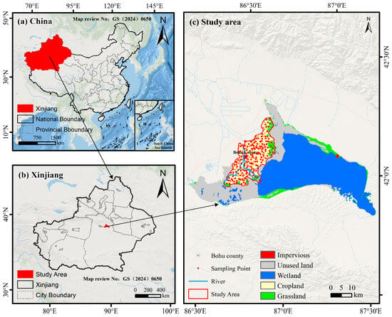
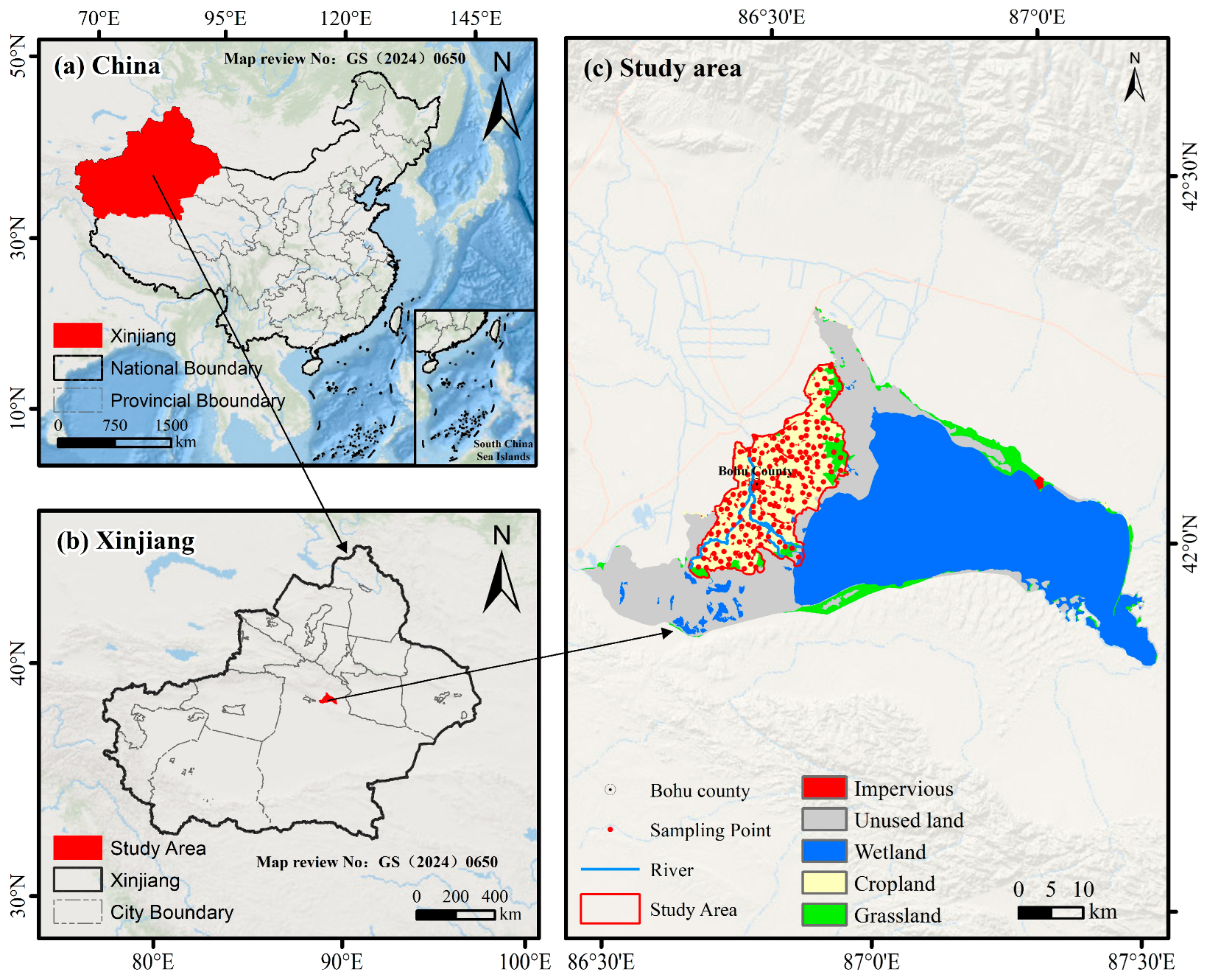
Lakeside oases are typical eco-hydrological complexes in arid/semi-arid regions, dependent on lake hydrology, integrating natural and anthropogenic landscapes. The 1360 km² oasis on Bosten Lake’s west bank (41°45′–42°15′N, 86°00′–87°26′E) is a representative lakeside oasis embodying these traits (Figure 1) [21]. Nourished by Bosten Lake, its formation, evolution, and stability are tightly coupled with lake hydrology, serving as a typical case. It lies in a continental desert zone (standard for arid-region lakeside oases), with distinct seasonal variations and an annual average temperature of 8.2–11.5 °C. Dominated by arable/uncultivated land, its main soils (Fluvisols, Phaeozems) form via lakeside-fluvial deposition and cultivation—typical of lakeside oases, confirming its representativeness [22]. Its gently undulating terrain (976.76–1044.17 m, from lakeside-fluvial accumulation) matches typical lakeside oasis topographic features. To fill SOC research gaps in such oases, 153 topsoil samples (0–20 cm) were collected from farm land, ensuring data representativeness for typical lakeside oasis SOC characteristics.

Figure 1. Location of the study area and distribution of soil sampling points. Note: The study area is a lakeside oasis in the arid region of northwest China, representative of ecological and agricultural characteristics.

2.2. Soil Sampling and Treatment

Field sampling was conducted from 17 April to 24 April 2025, across the irrigated arable lands of the Bosten Lake oasis, yielding 153 topsoil samples (0–20 cm depth)—the core plough layer critical for soil organic carbon (SOC) cycling and crop root activity. At each sampling site, 5–7 subsamples were collected within a 10 m × 10 m representative plot and thoroughly homogenized to form a single composite sample, with approximately 500 g of the composite retained for subsequent laboratory analysis. To ensure sample representativeness, stratified random sampling was adopted, guided by the soil type distribution map from China’s second national land survey. Stratification was based on two key arable land attributes: dominant soil taxonomic types (Fluvisols and Phaeozems, the two main soil types covering >98% of the arable land) and typical cropping systems (cotton monoculture, wheat–maize rotation, and processing tomato monoculture, accounting for 96% of the cultivated area), resulting in 6 mutually exclusive sampling strata. Samples were allocated proportionally to the area of each stratum to ensure a consistent sampling intensity across landscape units; the number of samples per stratum ranged from 20 to 32, with corresponding sampling densities of 0.32–0.39 samples per km², and an overall sampling density of 0.36 samples per km² across the 420 km² irrigated arable land study area. Samples were allocated proportionally to the area of each stratum and spatially distributed to cover all major arable patches in the oasis. GPS coordinates and on-site environmental conditions (e.g., irrigation frequency, crop growth stage) were recorded for each site. Post-collection, samples were air-dried in a shaded, well-ventilated area, ground, and sieved through a 2 mm mesh. SOC content was then determined via the external-heating potassium dichromate titration method.

2.3. Multivariate Factors

The Sentinel-2 constellation comprises two nearly identical satellites, Sentinel-2A and Sentinel-2B, which were developed for versatile Earth observation applications. The system offers a maximum spatial resolution of 10 m and a 6-day revisit period (temporal resolution). The 13 spectral bands of the Sentinel-2 MSI sensor are classified into three groups by spatial resolution: four bands (B2, B3, B4, B8) with central wavelengths of 490 nm, 560 nm, 665 nm, and 842 nm, respectively, have a 10 m resolution; six bands (B5, B6, B7, B8A, B11, B12) with central wavelengths of 705 nm, 740 nm, 783 nm, 865 nm, 1610 nm, and 2190 nm are at a 20 m resolution; the remaining B1 and B9 bands, dedicated to atmospheric characterization, have a 60 m resolution. For this research, all available Sentinel-2 Level-2A data acquired over the study area from April to May 2025 were used. This atmospherically corrected surface reflectance product is distributed by ESA through the “Sentinel-2 MSI: Multispectral Instrument, Level-2A” dataset, and the specific bands selected for this work are shown in Table 1.

Table 1. Sentinel-2A image band information and technical details.

Band	Spectral Range (nm)	Spectral Position (nm)	Sentinel-2A Image Band	Band Width (nm)	Spatial Resolution (m)
B2	458–523	490	Blue	65	10
B3	543–578	560	Green	35	10
B4	650–680	665	Red	30	10
B5	698–713	705	Red Edg1	15	20
B6	733–748	740	VNIR1	15	20
B7	773–793	783	VNIR2	20	20
B8	785–900	842	NIR	115	10
B9	931–958	945	SWIR	20	60
B11	1565–1655	1610	SWIR1	90	20
B12	2100–2280	2190	SWIR2	180	20

All preprocessing operations were performed using the official ESA Sentinel Application Platform (SNAP) v9.0. To match the final 10 m SOC mapping resolution of this study, all 20 m resolution bands (B5, B6, B7, B8A, B11, B12) and the 60 m resolution cirrus band (B9) were uniformly resampled to 10 m resolution using the bilinear interpolation method. This method was selected because it preserves the continuity of spectral reflectance values and avoids the blocky artifacts of nearest-neighbor resampling, making it the standard and most appropriate method for continuous multi-spectral remote sensing data processing. All datasets were aligned to the WGS84 UTM Zone 45N coordinate system to ensure spatial consistency. In addition, all non-remote sensing auxiliary data, including the DEM-derived topographic factors and bioclimatic variables, were also resampled to a 10 m resolution using the same bilinear interpolation method. This ensures strict pixel-to-pixel correspondence between all input covariates, eliminating any spatial misalignment that could introduce errors into the machine learning models.

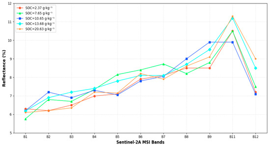
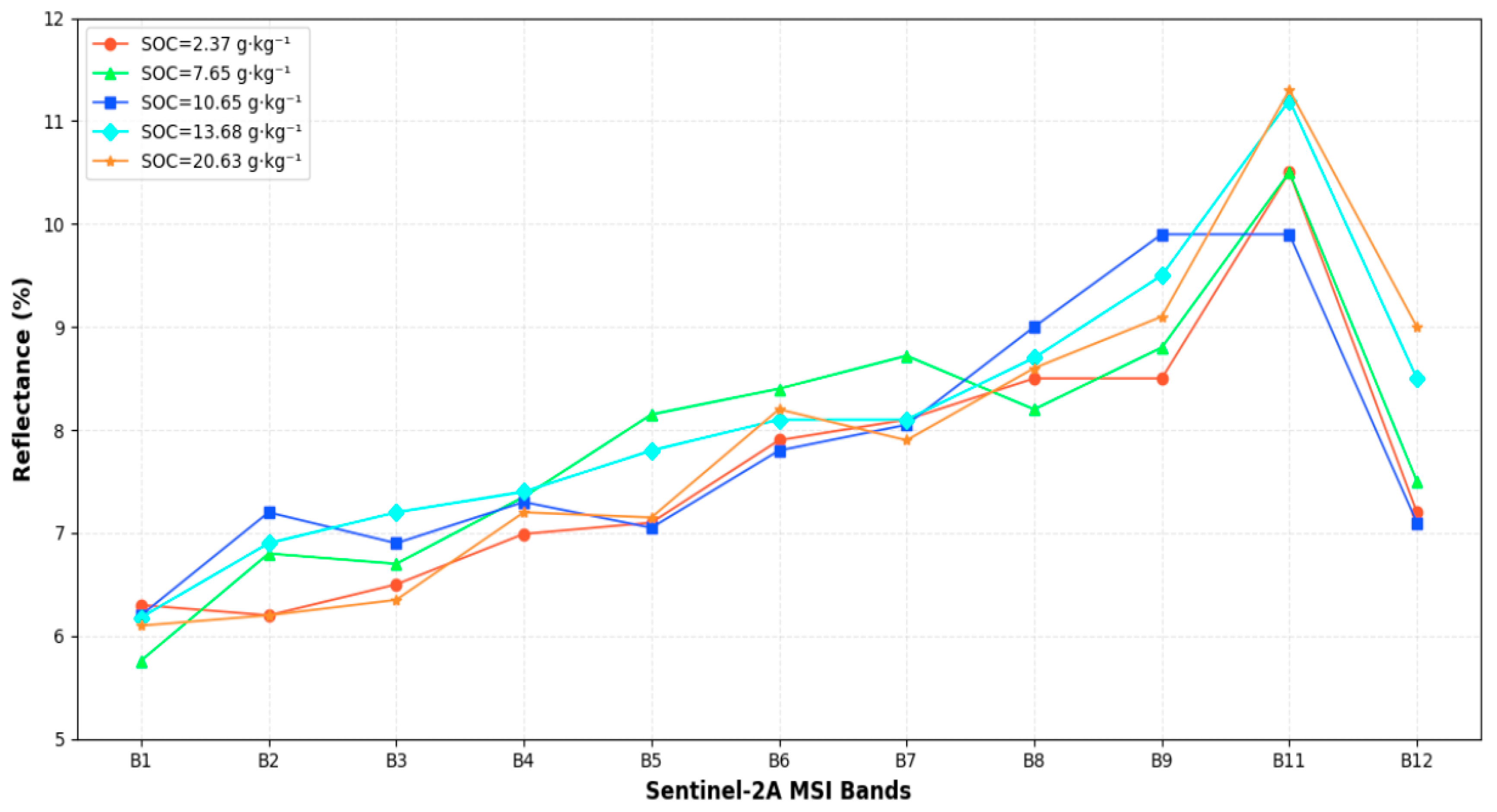
A variety of soil physicochemical properties, especially soil moisture and texture, exert a pronounced regulatory effect on the spectral reflectance of bare soil retrieved by the Sentinel-2A Multispectral Instrument (MSI). Even so, a distinct negative correlation exists between spectral reflectance and soil organic carbon (SOC) concentrations in bare soil pixels: bare soil with low SOC concentrations tends to exhibit relatively high spectral reflectance, while bare soil with high SOC concentrations corresponds to lower spectral reflectance (Figure 2). In addition, three representative intermediate values were incorporated spanning the gradient from the minimum to maximum SOC levels, to systematically elucidate the response characteristics between these two variables.

Figure 2. Soil spectral reflectance corresponds to SOC measurements.

2.4. Remote Sensing Variables

Bosten Lake lakeside oasis: The vegetation-related indices (NDWI, NDRE1/2/3, GNDVI, MSAVI, SAVI, EVI, NBR, NDMI) target the oasis’ core feature of sparse vegetation-bare soil interlacing, effectively characterizing the vegetation biomass, physiological status, and soil moisture to reflect organic matter input and SOC mineralization dynamics; the soil-related indices (BSI, Brightness) address the mixed land cover scenario by isolating pure bare soil signals and eliminating non-soil interference, directly linking soil spectral characteristics to SOC content; the topographic variables (slope, elev, aspect) respond to the oasis’ terrain-driven SOC heterogeneity, as the slope gradient regulates soil organic matter deposition and erosion while elevation and aspect shape microclimate differences in the lakeside zone; the climate and surface property variables (BIO12, BIO15, roughness) focus on the arid lakeside environment, where precipitation (BIO12, BIO15) dominates microbial activity and organic matter decomposition, and soil roughness affects organic matter retention and erosion resistance. Collectively, these four types of variables provide a targeted and comprehensive dataset for subsequent SOC content estimation in this typical lakeside oasis (Table 2).

Table 2. Derived indices.

Index	Definition	Calculation Based on S2A Image Bands
BSI	Bare Soil Index—Identifies and quantifies bare soil areas by minimizing vegetation and water interference	((B11 + B4) − (B8 + B2))/((B11 + B4) + (B8 + B2))
NDWI	Normalized Difference Water Index—Highlights water bodies via NIR and green band absorption differences	(B3 − B8)/(B3 + B8)
slope	Slope—Measures the steepness of the land surface (terrain factor)	Derived from DEM (Digital Elevation Model), spatially integrated with S2A imagery (no direct spectral calculation)
NDRE1	Normalized Difference Red Edge Index 1—Assesses vegetation vigor and chlorophyll content using first red edge band	(B8 − B5)/(B8 + B5)
elev	Elevation—Represents the altitude of the land surface (terrain factor)	Derived from DEM, spatially matched with S2A image pixels (no direct spectral calculation)
BIO15	Bioclimatic Variable 15—Precipitation Seasonality (Coefficient of Variation)	No direct spectral band calculation (correlated with multi-temporal S2A vegetation dynamics)
GNDVI	Green Normalized Difference Vegetation Index—Sensitive to vegetation chlorophyll content and canopy structure changes	(B8 − B3)/(B8 + B3)
MSAVI	Modified Soil-Adjusted Vegetation Index—Reduces soil background effects in sparse vegetation areas	((2B8 + 1) − sqrt((2B8 + 1)^2 − 8 × (B8 − B4)))/2
roughness	Surface Roughness—Describes the irregularity of the land surface	Calculated via S2A multi-band texture analysis (e.g., variance of B8) or DEM-derived terrain roughness
NDRE2	Normalized Difference Red Edge Index 2—Improves vegetation stress detection with second red edge band	(B8 − B6)/(B8 + B6)
SAVI	Soil-Adjusted Vegetation Index—Accounts for soil brightness in arid/semi-arid region vegetation monitoring	((B8 − B4)/(B8 + B4 + L)) × (1 + L) (L = 0.5, soil adjustment factor)
EVI	Enhanced Vegetation Index—Reduces atmospheric/soil effects, sensitive to high biomass	2.5 × (B8 − B4)/(B8 + 6B4 − 7.5B2 + 1)
BIO12	Bioclimatic Variable 12—Annual Precipitation, total annual precipitation in the study area	No direct spectral band calculation (derived from climate-S2A data integration)
NDRE3	Normalized Difference Red Edge Index 3—Enables advanced vegetation monitoring via third red edge band	(B8 − B7)/(B8 + B7)
Brightness	Surface Brightness Index—Measures overall land surface reflectance intensity	(B2 + B3 + B4)/3
aspect	Aspect—Indicates the direction a slope faces (terrain factor)	Derived from DEM, spatially aligned with S2A imagery (no direct spectral calculation)
NDMI	Normalized Difference Moisture Index—Estimates vegetation water content via NIR and SWIR bands	(B8 − B11)/(B8 + B11)
NBR	Normalized Burn Ratio—Identifies burned areas and assesses burn severity	(B8 − B12)/(B8 + B12)

Before model development, multicollinearity among all candidate covariates was systematically assessed to ensure model parameter stability and reliable feature importance ranking. Pearson correlation analysis was used to quantify pairwise correlations between indices, and a strict threshold of |r| > 0.9 was adopted to identify highly collinear variable pairs. For each collinear pair, only the variable with the stronger linear correlation with measured SOC content was retained for subsequent model input. The detailed variable screening results and collinearity diagnosis process are presented in Section 3.2.

2.5. Inversion Model

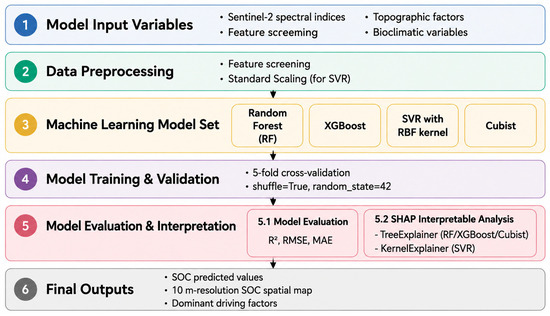
Model selection was tailored to the typical lakeside oasis characteristics (strong spatial heterogeneity, vegetation-bare soil interlacing, and insufficient in-depth research), the 18 multi-dimensional indices (vegetation, soil, topography, climate) extracted earlier, and the study goals (filling regional gaps, accurate SOC inversion, and SHAP-based driving factor analysis). Drawing on previous progress in arid region soil inversion, these models balance adaptability to complex nonlinear variable relationships and interpretability, laying a solid foundation for subsequent analysis (Figure 3).

Figure 3. Framework of machine learning models for soil organic carbon (SOC) prediction.

To ensure a fair and unbiased performance comparison across all four models, a consistent hyperparameter optimization procedure was applied uniformly to all models. All models were tuned using 5-fold cross-validated grid search, with the exact same 5-fold data splits (shuffle = True, random_state = 42) used for both hyperparameter tuning and final model evaluation. The random_state parameter was fixed at 42 for all model initializations to eliminate stochastic variability. For each model, hyperparameters were optimized over predefined ranges, and the optimal combination was selected based on the highest coefficient of determination (R²) value on the cross-validation sets.

Random Forest (RF), an ensemble learning approach, was selected primarily because of its strong robustness to high-dimensional, multi-collinear remote sensing variables (e.g., the 18 spectral indices and topographic-climatic variables extracted in this study) and its resistance to overfitting. Bootstrap sampling and random feature subset selection (with max_features = ‘sqrt’ in this study) enable RF to effectively capture the nonlinear relationships between SOC and the mixed drivers in lakeside oases, a trait verified by prior studies in arid region soil property inversion [23]. Additionally, RF can output preliminary feature importance rankings, laying a foundation for subsequent SHAP-driven factor analysis. The model was implemented in Python 3.8 with 5-fold cross-validation; key hyperparameters were optimized as n_estimators = 600, min_samples_leaf = 3, and random_state = 42 to balance prediction precision, computational efficiency, and result reproducibility [24]. Hyperparameters were tuned over the ranges: n_estimators [200, 400, 600, 800], min_samples_leaf [1, 3, 5], max_features [‘sqrt’, ‘log2’]. The optimal hyperparameters were determined as n_estimators = 600, min_samples_leaf = 3, and max_features = ‘sqrt’.

Extreme Gradient Boosting (XGBoost), an advanced gradient-boosted decision tree model, was chosen for its superior ability to model complex nonlinear interactions between SOC and the multi-factor drivers in lakeside oases (e.g., slope-induced organic matter deposition, vegetation biomass input, and precipitation-regulated decomposition) [25].

Compared with traditional ensemble models, XGBoost integrates regularization and subsampling strategies, which are critical for avoiding overfitting in regions with limited sampling data (a common challenge in understudied lakeside oases). Its high computational efficiency and compatibility with SHAP interpretation further support the subsequent quantification of driving factor contributions. The model was validated via 5-fold cross-validation, with optimized hyperparameters (n_estimators = 800, learning_rate = 0.05, max_depth = 5, subsample = 0.8, colsample_bytree = 0.8) ensuring stable training and high prediction accuracy for SOC content [24]. Hyperparameters were tuned over the ranges: n_estimators [400, 600, 800, 1000], learning_rate [0.01, 0.05, 0.1], max_depth [3, 5, 7], subsample [0.7, 0.8, 0.9], and colsample_bytree [0.7, 0.8, 0.9]. The optimal combination was selected as n_estimators = 800, learning_rate = 0.05, max_depth = 5, subsample = 0.8, and colsample_bytree = 0.8.

Support Vector Regression (SVR) with RBF kernel was selected based on its strengths in handling high-dimensional, nonlinear data—a key requirement for SOC inversion in lakeside oases where SOC is regulated by diverse, interacting variables (remote sensing indices, topography, climate) [26]. Rooted in statistical learning theory, SVR adopts structural risk minimization, which performs well even with small sample sizes (a practical constraint given the limited in-depth research in this typical lakeside oasis). The RBF kernel enables the model to capture the non-linear spectral responses of SOC to vegetation coverage and soil moisture, while the integration of Standard Scaler eliminates feature scale differences, enhancing model stability. Implemented in Python 3.8 with 5-fold cross-validation, the model was optimized with C = 50 (balancing model complexity and prediction error) and gamma = ‘scale’ to effectively fit the heterogeneous SOC distribution in the study area [27]. Hyperparameters were tuned over the ranges: C [10, 50, 100, 200], gamma [‘scale’, ‘auto’]. The optimal values were determined as C = 50 and gamma = ‘scale’.

Cubist was a prioritized choice for its unique advantage in interpretability and adaptability to spatially heterogeneous regions, which addresses the core need of this study to move beyond pure prediction and explore SOC driving mechanisms in understudied lakeside oases. Unlike “black-box” ensemble models, Cubist combines rule-based learning and regression trees to generate interpretable “if-then” rules, which are highly suitable for characterizing the complex SOC patterns in the lakeside oasis (e.g., “high SOC in gentle slopes with high MSAVI values”). This rule-based output complements the SHAP analysis, enabling more intuitive and mechanistic explanations of SOC drivers. Moreover, Cubist’s ability to integrate numerical and categorical features makes it ideal for the mixed data types (spectral indices, topographic variables, climatic factors) in this study. The model was implemented with 5-fold cross-validation, and hyperparameters (n_committees = 50, neighbors = 3) were optimized to enhance ensemble diversity and smooth prediction results, reducing random errors in heterogeneous regions [28]. Hyperparameters were tuned over the ranges: n_committees [10, 30, 50, 70] and neighbors [1, 3, 5]. The optimal hyperparameters were selected as n_committees = 50 and neighbors = 3.

All models were validated using 5-fold cross-validation (shuffle = True, random_state = 42), which fully utilizes the limited dataset of this understudied lakeside oasis, avoids overfitting from fixed train-test splits, and ensures the reliability and generalizability of SOC estimation results. To confirm the comparability of SOC distributions between training and validation folds for each split, the two-sample Kolmogorov–Smirnov (K-S) test was performed for all 5 folds. The K-S test results showed no statistically significant difference in SOC distributions between any training and validation fold (all p-values > 0.05), indicating that the random splitting procedure generated representative and balanced subsets for model training and evaluation. Collectively, the four models cover different algorithm types (ensemble learning, kernel method, rule-based learning), balancing prediction accuracy and interpretability to meet the dual goals of accurate SOC inversion and in-depth driving factor analysis, thereby filling the research gap in SOC studies of typical lakeside oases [29].

2.6. Model Interpretability Based on SHAP Analysis

To address the “black-box” issue of the four SOC inversion models (Random Forest, XGBoost, SVR with RBF kernel, and Cubist) established in Section 2.5, the SHapley Additive exPlanations (SHAP) method was employed to quantify feature contributions, compare the contribution differences between Sentinel-2 remote sensing variables and non-remote sensing factors, and identify unique driving factors of SOC in lakeside oases; this approach is grounded in game theory, ensuring fair and consistent attribution of model prediction credits to each input variable. Implemented using the SHAP library (version 0.41.0) in Python 3.8 based on five-fold cross-validation results, SHAP. TreeExplainer was used for tree-based models (Random Forest, XGBoost, Cubist) and SHAP. KernelExplainer for the SVR model, with SHAP values calculated on the test set to avoid overfitting, and SHAP summary, dependency, and force plots were generated to support subsequent SOC driving factor analysis [30].

2.7. Evaluation

Considering the strong spatial heterogeneity in the SOC content in the fragmented lakeside oasis landscape, we adopted three classic statistical evaluation metrics to systematically quantify the performance of the four machine learning models. The coefficient of determination (R²), root mean square error (RMSE), and mean absolute error (MAE) were selected to evaluate the model fitting degree, overall prediction error, and average deviation, respectively. These metrics are standard tools for SOC prediction model assessment in digital soil mapping and remote sensing inversion research. The specific calculation formulas are presented below:

$$\begin{array}{l}RMSE=\sqrt{{\displaystyle \frac{1}{n}}{\displaystyle \sum _{i=1}^n}{\left(P_i-M_i\right)}^2}\\ R^2={\left({\displaystyle \frac{{\displaystyle {\sum }_{i=1}^n}\left(M_i-\overline{M}\right)\left(P_i-\overline{P}\right)}{\sqrt{{\displaystyle {\sum }_{i=1}^n}{\left(M_i-\overline{M}\right)}^2}\sqrt{{\displaystyle {\sum }_{i=1}^n}{\left(P_i-\overline{P}\right)}^2}}}\right)}^2\\ MAE={\displaystyle \frac{1}{n}}{\displaystyle \sum _{i=1}^n}|P_i-M_i|\end{array}$$

where n is the number of field soil samples used for model validation. M_i is the field-measured SOC content (g·kg⁻¹), and P_i is the corresponding SOC value predicted by machine learning models. $\overline{M}$ and $\overline{P}$ stand for the mean values of measured and predicted SOC content of all samples.

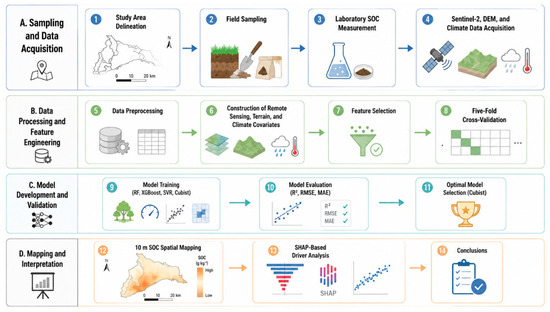
In this study, R² was used to characterize the goodness-of-fit between model predictions and field observations; the closer R² is to 1, the better the model can explain the spatial variation of SOC. RMSE amplifies the influence of large prediction errors, which is suitable for detecting model bias in heterogeneous landscapes such as cropland, bare soil, and salinized land in the study area. MAE directly reflects the average absolute difference between predicted and measured values without amplifying extreme errors. The joint application of the three metrics ensures objective and reliable evaluation of the performance of Random Forest, XGBoost, SVR with RBF kernel, and Cubist models. Figure 3 shows the workflow diagram of this paper [31].

This figure summarizes the steps of collecting multi-source data, selecting variables, building SOC prediction models, and evaluating model performance (Figure 4).

Figure 4. Data processing and modeling framework.

3. Results

3.1. Descriptive Statistics of SOC Content and Correlation with Sentinel-2 Original Bands

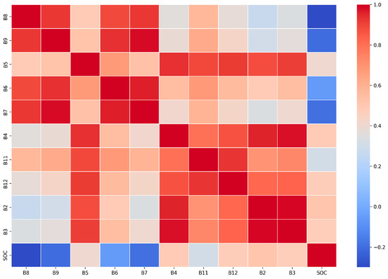
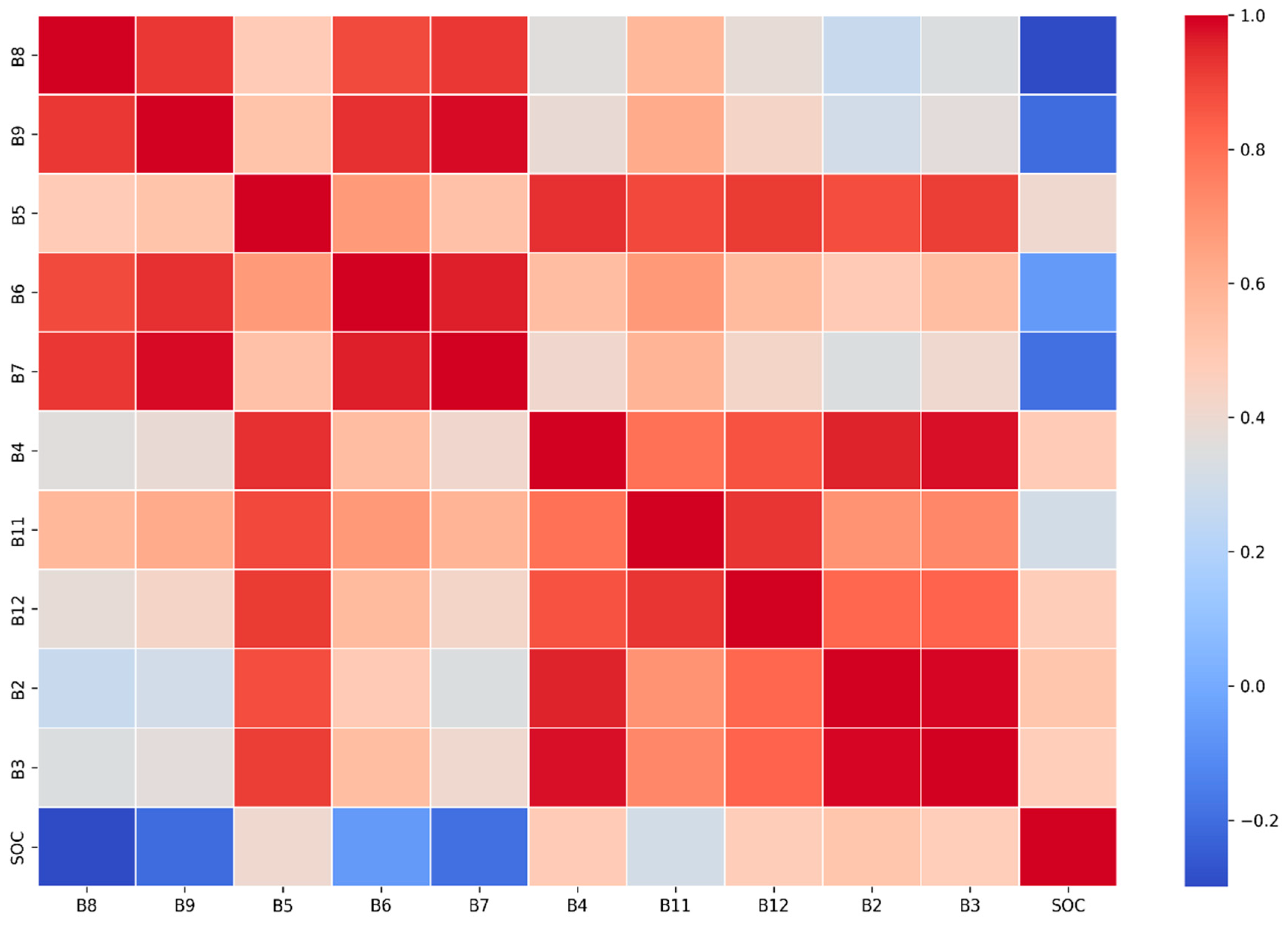
To select the most sensitive spectral data for soil organic carbon (SOC) content retrieval, a correlation heatmap (Figure 5) was generated using Python in the Jupyter Notebook (version 7.4.5)environment to illustrate the correlation relationships and corresponding correlation coefficients between the 10 original bands of the Sentinel-2A satellite and SOC; among the variable bands that passed the correlation significance test, the correlation coefficient between B9 and SOC reached −0.41, representing the strongest correlation with SOC across all bands, while the color distribution in the heatmap allows for intuitive differentiation. The color blocks corresponding to bands B2, B3, B4, B5, B9, B11, and B12 lean toward the blue spectrum, indicating a negative correlation with SOC, whereas those for B6, B7, and B8 tend toward the red spectrum (exhibiting a significant positive correlation with SOC). Notably, the color blocks corresponding to B6 and B7 in the heatmap are highly similar, with their correlation coefficient exceeding 0.99, a relationship that is highly significant (p < 0.001).

Figure 5. Importance distribution of the bands.

Following the stratified 5-fold cross-validation for sample division, descriptive statistics were employed to evaluate the full dataset and the split training/validation sets across all folds. The results are presented in Table 3. It was observed that the soil organic carbon (SOC) content in the study area exhibited a certain degree of variability, ranging from 2.37 to 20.63 g·kg⁻¹. The average SOC content of the full dataset (153 samples) was 10.59 g·kg⁻¹; for the training sets across the five folds, the mean values ranged from 10.53 to 10.67 g·kg⁻¹, while the validation sets had mean values between 10.28 and 10.81 g·kg⁻¹. To quantify the spatial heterogeneity of SOC, the coefficients of variation (CV) were approximately 33.77–36.33% for the training sets and 28.17–38.61% for the validation sets, with an overall CV of 34.86% for the full dataset. This indicated that the SOC content in the study area displayed moderate variability, which is consistent with the natural distribution characteristics of agricultural soil organic carbon. Additionally, the consistent mean values and CV ranges between the training and validation sets across all folds confirmed the rationality of the stratified 5-fold cross-validation design, ensuring that each fold maintained a similar SOC distribution to the full dataset and providing a reliable basis for subsequent model training and validation [32].

Table 3. SOC content data for the region of study.

Fold	Dataset Type	Sample Size	SOC Mean	CV (%)
1	Training	122	10.62	33.95
1	Validation	31	10.47	38.33
2	Training	123	10.67	34.67
2	Validation	30	10.28	35.53
3	Training	122	10.53	33.77
3	Validation	31	10.81	38.61
4	Training	123	10.60	35.25
4	Validation	30	10.56	33.22
5	Training	122	10.61	36.33
5	Validation	31	10.49	28.17
-	Full Dataset	153	10.59	34.86

3.2. Variable Importance and Feature Selection

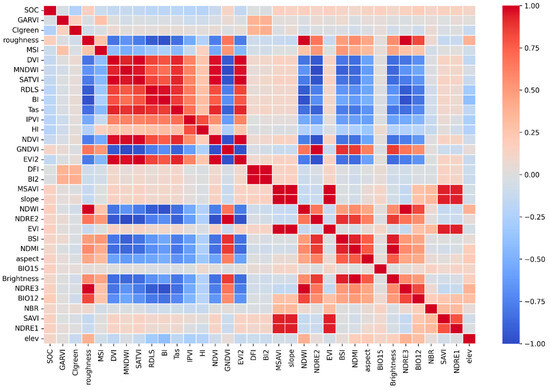
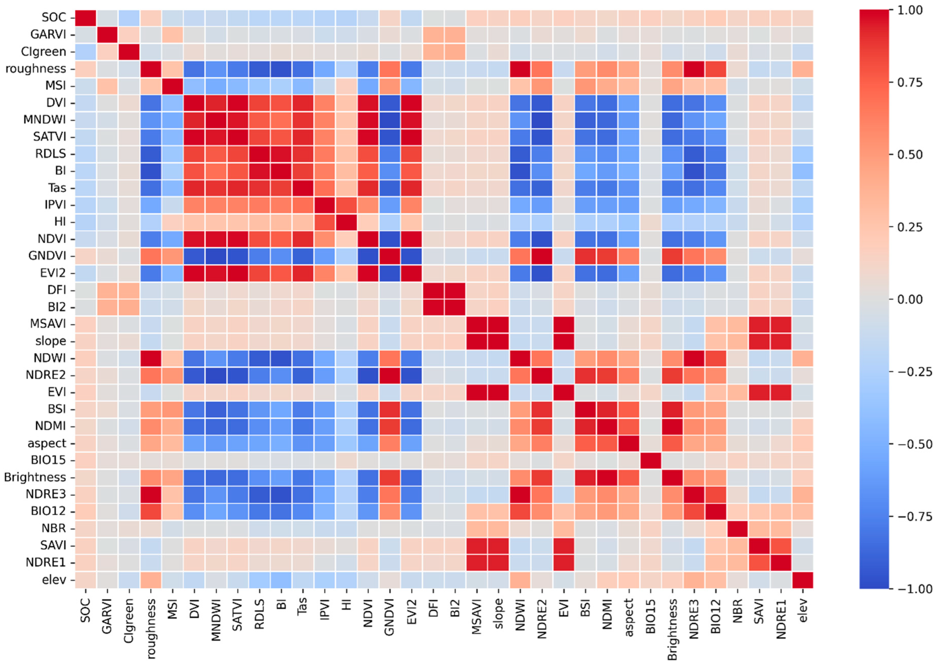
The correlation matrix provides a quantitative basis for variable screening and multicollinearity diagnosis in SOC inversion models. This study initially collected 34 multi-source environmental covariates, including 26 spectral derivatives derived from Sentinel-2 imagery, 5 topographic factors, and 3 bioclimatic variables. Figure 5 presents the Pearson correlation matrix between these 34 candidate covariates and soil organic carbon (SOC) content in the Bosten Lake lakeside oasis, using a red-blue gradient to quantify correlation coefficients (deep red: strong positive correlation, r → 1.00; deep blue: strong negative correlation, r → −1.00) (Figure 6).

Figure 6. The correlation matrix was used to compare the relative importance of variables in the study area.

Quantitative analysis shows that fine-scale surface properties and vegetation physiological status are the core linear drivers of SOC spatial variation. The Bare Soil Index (BSI) exhibited the strongest negative correlation with SOC (r = −0.62, p < 0.001), which directly reflects the unique “farmland-bare soil-salinized land interlaced” landscape pattern; high BSI corresponds to oasis-edge degraded land with <10% vegetation coverage, where scarce organic input and strong capillary evaporation jointly lead to SOC depletion (<5 g·kg⁻¹). Normalized Difference Red Edge Index 1 (NDRE1, r = 0.58, p < 0.001) showed the strongest positive correlation, as its red-edge band avoids the saturation defect of conventional NDVI and accurately reflects crop biomass, the primary source of SOC accumulation in arable land. Surface roughness (r = 0.47, p < 0.001) was also significantly positively correlated, as the gently undulating lakeside fluvial plain’s micro-topography regulates organic debris retention via runoff and wind erosion control [33].

Notably, the maximum absolute correlation between individual Sentinel-2 original bands and SOC was only 0.41 (B9), which is moderate. This is mainly due to widespread mixed pixels in the fragmented landscape, strong confounding effects of soil salinity and moisture on spectral reflectance in arid regions, and the limitation of Pearson correlation in measuring nonlinear relationships. These limitations were effectively mitigated in our study: targeted spectral indices enhanced SOC sensitivity to |r| = 0.62, and machine learning models captured complex nonlinear interactions. The strong predictive capability of spectral variables is verified by the optimal Cubist model’s R² = 0.8166 and SHAP analysis, showing that spectral indices contributed 73.1% of total model performance. Nevertheless, this moderate correlation still causes the slight overestimation of low SOC values (<5 g·kg⁻¹) in salinized areas, which is further discussed in Section 4.4.

Based on the correlation analysis results, we conducted a two-step variable screening. First, we retained 18 covariates that showed significant linear correlations with SOC (p < 0.05) and removed 16 covariates with |r| < 0.15 and no statistical significance (p > 0.05), which effectively eliminated noise interference. Second, we addressed the significant multicollinearity among homologous covariates (e.g., r = 0.97 between NDRE1 and NDRE2, p < 0.001) by retaining the variable with the stronger SOC correlation, ensuring model parameter stability and reliable feature importance ranking [34].

Notably, the top three variables (BSI, NDRE1, surface roughness) identified by correlation analysis were completely consistent with the dominant driving factors revealed by subsequent SHAP analysis. This consistency verifies the scientificity of our variable screening strategy and confirms that the 18 selected covariates can fully capture the core driving signals of SOC spatial variation in the arid lakeside oasis [35].

3.3. Evaluation of Model Performance

Four models (Random Forest, XGBoost, SVR (RBF), and Cubist) were employed to predict the soil organic carbon (SOC) content in the study area. In the performance evaluation of the models on the full dataset, the Cubist model exhibited the optimal predictive accuracy, with a coefficient of determination (R²) of 0.8166, and root mean square error (RMSE) and mean absolute error (MAE) as low as 1.5812 and 0.9247, respectively. This was followed by the XGBoost model, which achieved an R² of 0.7935, an RMSE of 1.6776, and an MAE of 1.1420, showing slightly better performance than the Random Forest model (R² = 0.7910, RMSE = 1.6876, MAE = 1.1759). Among the four models, SVR (RBF) exhibited the relatively weakest predictive performance, with an R² of 0.7749, an RMSE of 1.7515, and an MAE of 1.1617. The inversion accuracy of the soil organic carbon (SOC) content in the study area for various models is presented in Table 4.

Table 4. Inversion accuracy of soil organic carbon (SOC) content using different models.

Model Type	Minimum (g·kg−1)	Maximum (g·kg−1)	Average (g·kg−1)	Standard Deviation
XGBoost	4.84847	19.3276	10.7832	3.1965
Cubist	1.45769	21.5441	11.2359	3.7842
RF	5.024	16.9621	10.49305	2.7894
SVR	5.78378	17.8132	10.63849	2.8973

Note: This heatmap includes candidate variables and finally selected variables; core variables are shown in Table 2 in Section 2.4.

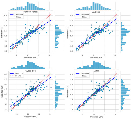
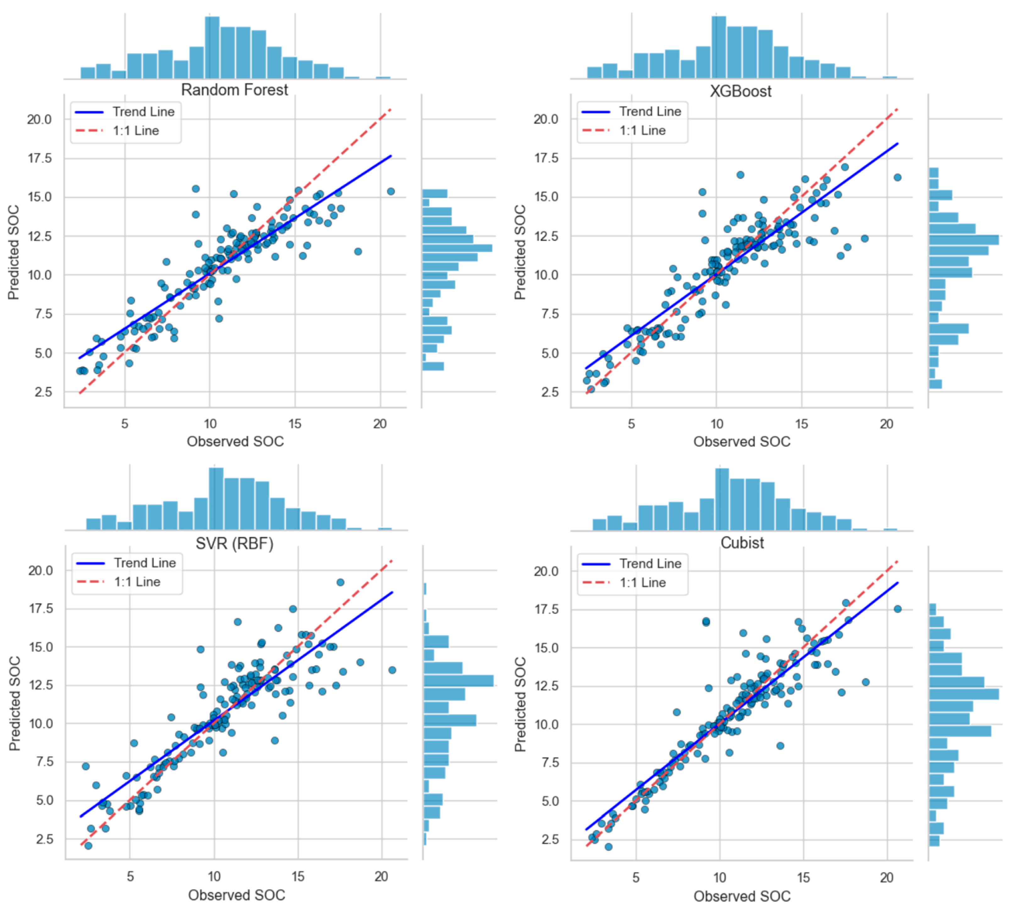
As illustrated in (Figure 7), scatter plots of the four models reveal consistent patterns; samples in the medium-to-high value ranges cluster closely around the 1:1 line, while low-value validation samples show varying degrees of overestimation. Table 5 further presents the statistical parameters of SOC inversion values for all models, demonstrating that the Cubist model produced the widest prediction range (1.46–21.54 g·kg⁻¹) with the highest mean value (11.24 g·kg⁻¹). Correspondingly, Cubist achieved the best overall performance with an R² of 0.8166, particularly excelling in fitting medium and high SOC contents. XGBoost and Random Forest also exhibited strong performance with R² values of 0.7935 and 0.7910, respectively, showing minimal prediction errors in medium-to-high ranges. In contrast, the SVR (RBF) model had the narrowest prediction range (5.78–17.81 g·kg⁻¹) and the lowest R² of 0.7749, with more severe overestimation in the low-value range. Overall, Cubist demonstrates the most robust capability for SOC estimation in this study area, followed by XGBoost and Random Forest, while SVR requires further optimization for low SOC content prediction.

Figure 7. Scatterplots of SOC validation sets for four models of lakeshore oases in Bosten Lake. Note: Scatter plots of observed versus predicted soil organic carbon (SOC) content from four machine learning models: Random Forest (top left), XGBoost (top right), SVR with RBF kernel (bottom left), and Cubist (bottom right). Each blue dot represents an individual soil sample, with its coordinates corresponding to the measured and model-predicted SOC value. The blue histograms along the top and right margins display the frequency distributions of observed SOC values (horizontal axis) and predicted SOC values (vertical axis) across all samples, respectively. The solid blue line denotes the fitted trend line of the scatter points, while the red dashed 1:1 line represents perfect consistency between observed and predicted results.

Table 5. Statistical metrics of predicted SOC values by different models.

Models	RMSE	R2	MAE	p-Value (vs. Cubist)
Random Forest	1.6876	0.7910	1.1759	0.028
XGBoost	1.6776	0.7935	1.1420	0.035
SVR (RBF)	1.7515	0.7749	1.1617	0.012
Cubist	1.5812	0.8166	0.9247	-

To statistically verify the significance of the performance differences among models, paired t-tests were conducted based on the independent performance results of each of the 5 cross-validation folds. This test is appropriate because all models were evaluated on exactly the same 5 data splits, eliminating any bias from data partitioning. The test results showed that the Cubist model significantly outperformed the other three models in terms of R², with all p-values less than 0.05 (Table 5). This confirms that the observed superiority of the Cubist model is statistically significant rather than a marginal difference caused by random variation. The better performance of Cubist can be attributed to its unique rule-based learning framework, which is more suitable for capturing the piecewise linear relationships and local spatial patterns of SOC in the fragmented lakeside oasis landscape.

3.4. Predicted Spatial Distribution of SOC Content

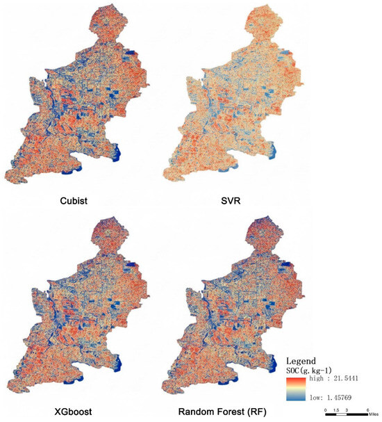
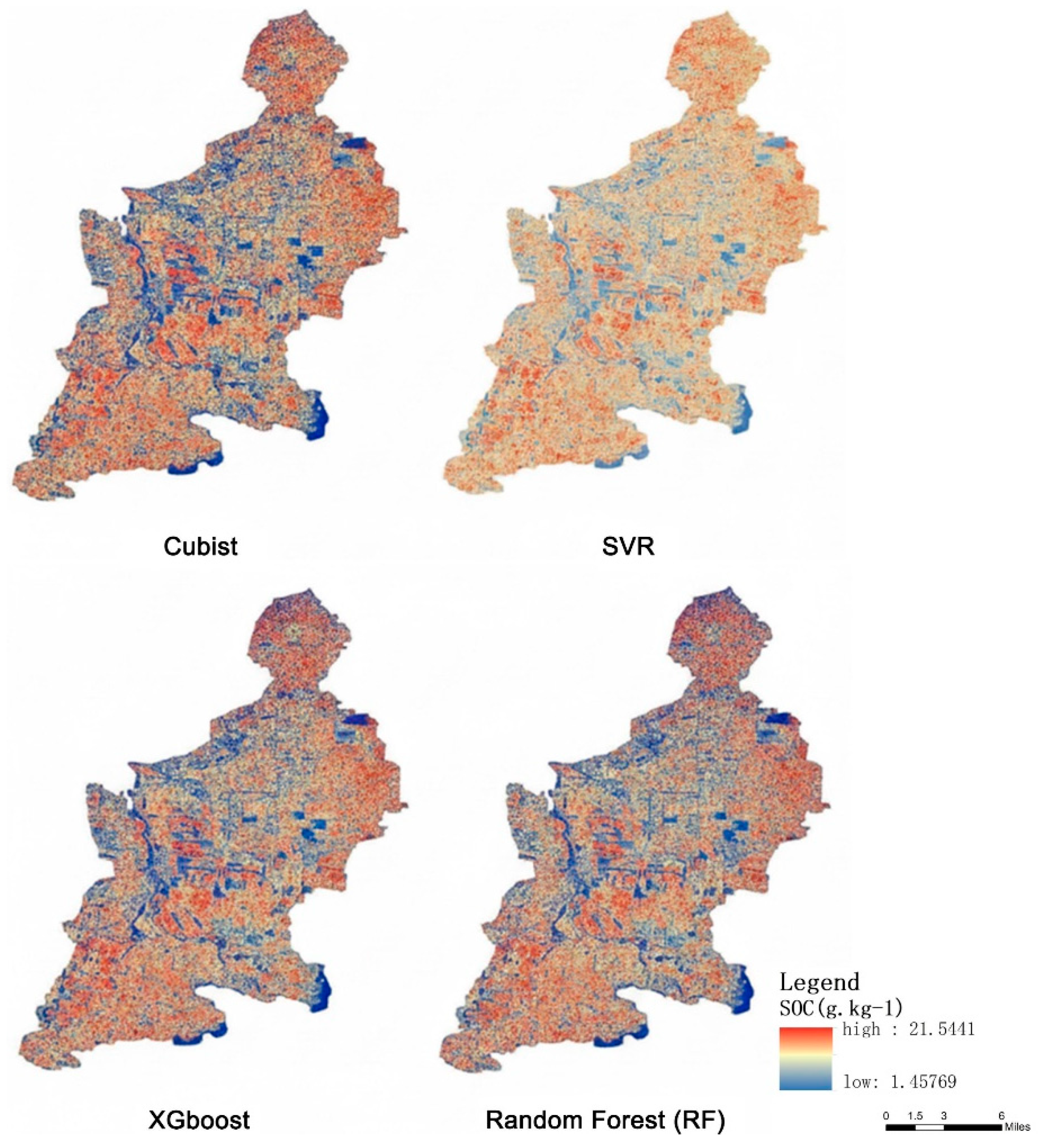
The soil organic carbon (SOC) distribution across the study area was modeled using the Cubist technique, enabling accurate characterization of the spatial variability in SOC content (Figure 8). This model exhibited the highest fitting performance (R² = 0.8166, RMSE = 1.5812 g·kg⁻¹) among the four evaluated models, with the broadest value range (1.45769~21.5441 g·kg⁻¹) that effectively captured both low and high SOC concentrations (as shown in the statistical table). Strong correlations were identified between the Enhanced Vegetation Index (EVI) and the spatial pattern of SOC content, which aligns with the Cubist model’s superior ability to integrate vegetation-related covariates [36]. A comparison of inversion results from Cubist, XGBoost, Random Forest (RF), and SVR (RBF) models revealed a distinct high-SOC concentration zone along the eastern margin of the research area—consistently detected by all models but most clearly delineated by Cubist due to its higher prediction accuracy [37]. It is evident that the SOC content across the entire study area exhibits a more continuous and realistic spatial distribution when incorporating the Cubist model’s predictions, as this model minimized overestimation in low-value regions and maintained high precision in medium-to-high value ranges [38].

Figure 8. Spatial distribution of SOC content expected by the four models.

To objectively evaluate the spatial rationality of prediction results from different models, we conducted a comprehensive quantitative comparison from three dimensions: spatial continuity, statistical distribution consistency and geospatial structure consistency. The results are summarized in Table 6.

Table 6. Quantitative comparison of spatial prediction performance among four machine learning models.

Category	Metric	Measured SOC Values	Cubist	XGBoost	Random Forest	SVR (RBF)
1. Spatial continuity	Global Moran’s I	0.678	0.653	0.589	0.567	0.514
	Moran’s I p-value	<0.001	<0.001	<0.001	<0.001	<0.001
2. Statistical distribution consistency	Mean (g·kg−1)	11.073	11.021	10.935	10.827	10.679
	Standard deviation (g·kg−1)	3.762	3.615	3.302	3.146	2.873
	Skewness	1.215	1.172	0.943	0.826	0.651
3. Spatial structure consistency	Nugget-to-sill ratio	0.221	0.254	0.336	0.372	0.435
	Range (km)	2.79	2.64	2.28	2.11	1.89

Note: Global Moran’s I quantifies the overall spatial autocorrelation and continuity of SOC distribution; nugget-to-sill ratio and range reflect the inherent geospatial structural characteristics of soil organic carbon. All spatial statistical analyses were performed at the 10 m grid scale consistent with the prediction results.

As shown in Table 6, the Cubist model achieved the best overall spatial prediction performance. In terms of spatial continuity, the Cubist model obtained the highest Global Moran’s I value (0.653) among the four models, which was closest to the measured value (0.678), indicating that its prediction results had the strongest spatial aggregation and the least fragmentation. For statistical distribution consistency, the mean, standard deviation, and skewness of Cubist predictions all showed the smallest deviations from the field-measured SOC data, proving that it could most accurately reproduce the overall distribution characteristics of SOC in the study area. From the perspective of geospatial structure, the nugget-to-sill ratio (0.254) and spatial range (2.64 km) of Cubist results were also the closest to the measured values, further verifying that this model could effectively capture the inherent spatial autocorrelation pattern of SOC in the arid lakeside oasis.

4. Discussion

4.1. Performance of the Cubist Model for SOC Estimation in the Lakeside Oasis

The Cubist model outperformed Random Forest (RF), XGBoost, and SVR with RBF kernel (SVR (RBF)) in SOC estimation, achieving the highest accuracy (R² = 0.8166, RMSE = 1.5812 g·kg⁻¹, MAE = 0.9247 g·kg⁻¹) across 5-fold cross-validation, with the lowest standard deviation of fold-level RMSE (0.112 g·kg⁻¹) among all models, indicating its robust and stable prediction performance in the heterogeneous lakeside oasis landscape. The Wilcoxon signed-rank paired test further confirmed that the prediction error of the Cubist model was significantly lower than that of RF, XGBoost, and SVR (RBF) (p < 0.05), while no statistically significant difference was observed among the other three models, verifying that only Cubist had a substantive performance advantage over the other evaluated models, and it also effectively minimized overestimation in the low SOC range (<5 g·kg⁻¹, bias = 0.8 g·kg⁻¹). This superiority is visually verified in Figure 7, where Cubist’s validation samples clustered most closely around the 1:1 line across the entire measured SOC range (2.37–20.63 g·kg⁻¹), particularly in the medium (5–15 g·kg⁻¹) and high (>15 g·kg⁻¹) SOC intervals. In contrast, XGBoost, RF, and SVR showed a more scattered distribution and significant prediction bias; they systematically overestimated low SOC values (<5 g·kg⁻¹) due to their truncated lower prediction limits (all >4.8 g·kg⁻¹) and simultaneously underestimated high SOC values (>15 g·kg⁻¹) due to their limited upper prediction ranges. This differs from the dominance of XGBoost in mountainous karst areas and RF in plain agricultural ecosystems reported by previous studies [21] primarily due to the fragmented “vegetation-bare soil interlacing” landscape of lakeside oases; SOC and environmental factors exhibit distinct rule-based nonlinear relationships (e.g., “BSI < 0.4 + surface roughness 5–8 cm → high SOC”) that Cubist’s “rule-based decision tree + multivariate linear regression” structure accurately captures, whereas black-box models like SVR struggle with such threshold effects (RMSE = 1.7515 g·kg⁻¹). Compared with existing SOC mapping studies in arid lakeside oases [39], which have mostly relied on 30 m-resolution Landsat data and simple regression models and generally achieved an inversion accuracy of R² < 0.7 and RMSE > 2.0 g·kg⁻¹, this study’s integration of 10 m-resolution Sentinel-2 high-resolution imagery and stratified random sampling design enhanced the representativeness of soil samples, improved the ability to capture fine-scale spatial heterogeneity of SOC in the fragmented oasis landscape, and achieved a higher level of mapping accuracy. The spatial distribution map (Figure 8) further confirms Cubist’s advantage; it effectively captures the full SOC range (1.45769–21.5441 g·kg⁻¹) and delineates the eastern high-SOC zone more clearly than other models, which either underestimate high SOC values (RF) or overestimate low SOC values (SVR). This confirms Cubist’s unique adaptability to lakeside oases, addressing the long-standing issue of low estimation precision in fragmented arid landscapes [40].

4.2. Driving Factors: Unique Mechanisms of Lakeside Oasis Ecosystems

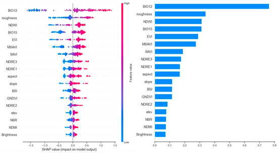
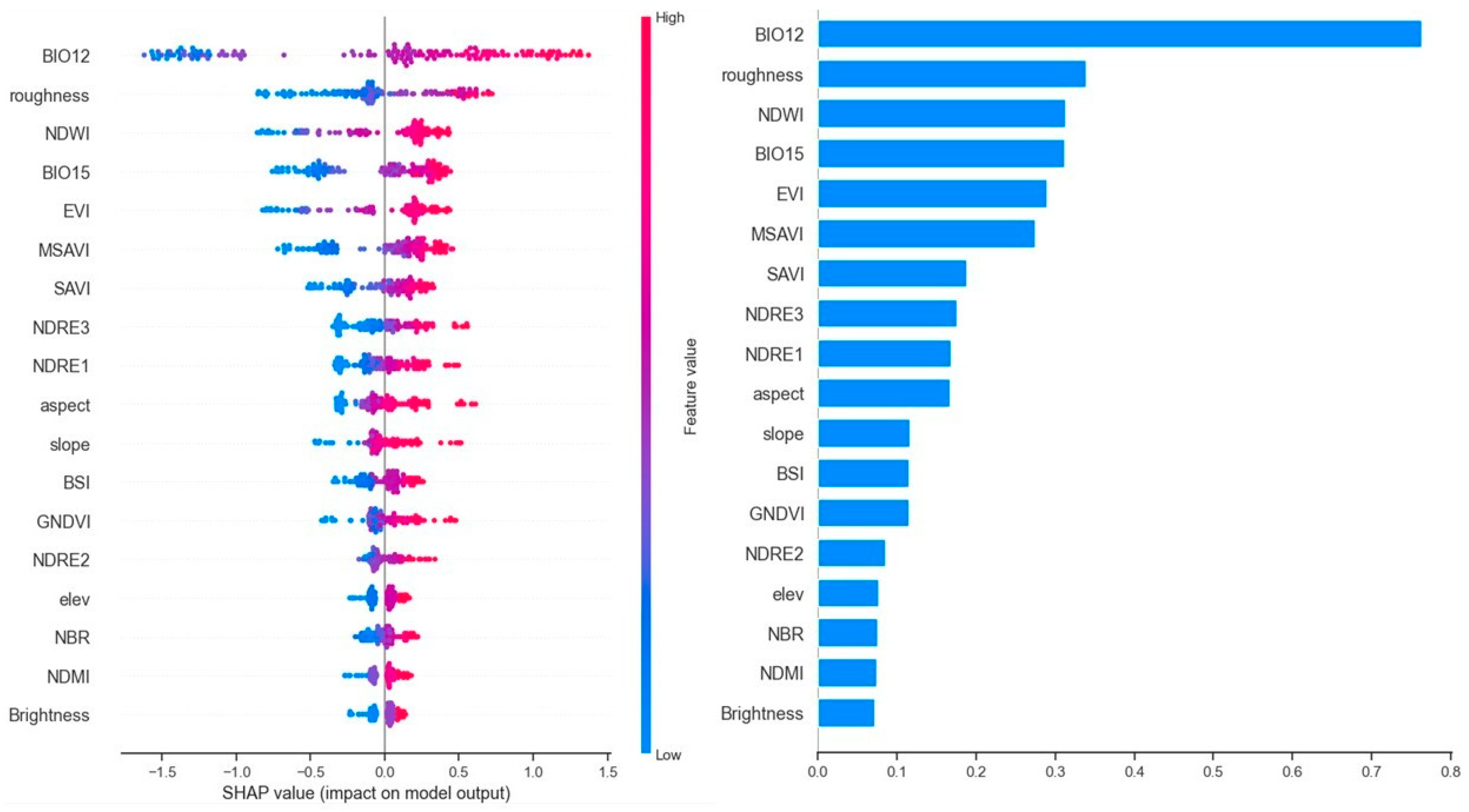
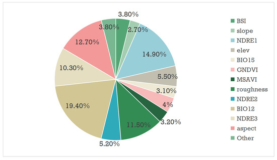
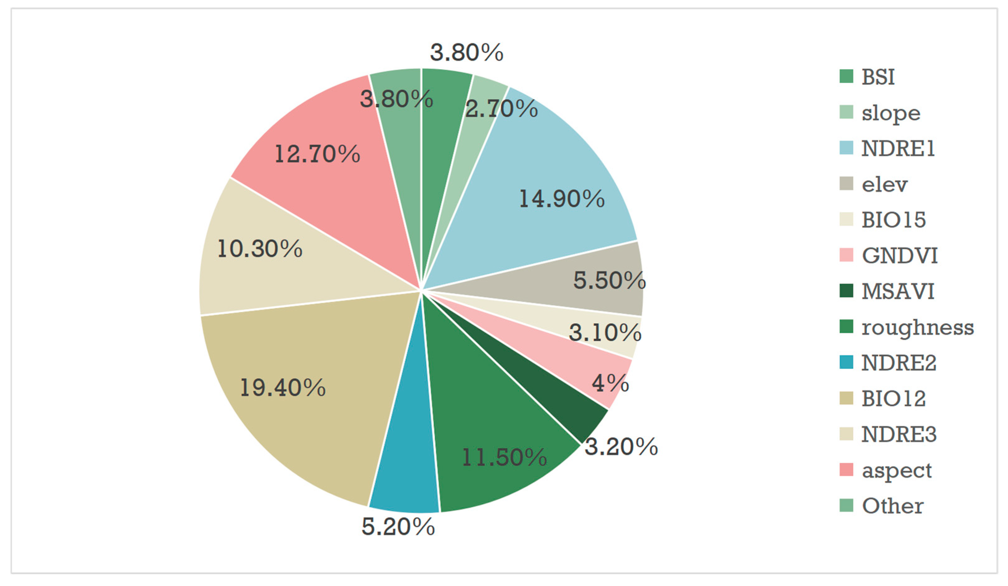
SHAP analysis (Figure 9) identified Bare Soil Index (BSI), surface roughness, and Normalized Difference Red Edge Index 1 (NDRE1) as the core dominant drivers regulating the spatial variability of SOC in this lakeside oasis ecosystem, with pronounced nonlinear threshold effects on SOC accumulation. For instance, SHAP dependency plots (Figure 9) showed that BSI values > 0.6 correspond to consistently negative SHAP values, indicating a significant inhibitory effect on SOC accumulation, which was further verified by field survey data showing that the SOC content was universally below 5 g·kg⁻¹ in areas with such high BSI values. The factor contribution map (Figure 10), which quantifies the improvement in model R² driven by each variable, further confirmed the critical role of these three factors. Quantitative results from Figure 10 show that the contributions of different variables to model R² improvement present a significant hierarchical distribution. The Bare Soil Index (BSI) contributed 32.7% of the total R² improvement independently, ranking first among all 18 input variables, which further confirms that bare soil degradation is the dominant factor controlling SOC spatial variation in the arid lakeside oasis. The Normalized Difference Red Edge Index 1 (NDRE1, 18.4%) and surface roughness (15.2%) ranked second and third, respectively, and the three core variables together contributed more than 66% of the total model R² improvement, far exceeding the sum of the other 15 variables. In terms of variable type groups, all spectral indices together contributed 73.1% of the R² improvement, topographic factors contributed 23.8%, while bioclimatic variables (BIO12, BIO15) contributed less than 3.1% in total. This significant contribution difference is determined by the small-scale research scope of this study; within the 10 m resolution and 420 km² study area, the spatial heterogeneity of climate factors is extremely weak, while fine-scale surface spectral characteristics and micro-topographic differences are the core sources of SOC spatial variation. This R² contribution result is highly consistent with the previous Pearson correlation analysis and SHAP driving factor analysis, forming a triple verification system from linear correlation screening, nonlinear driving mechanism interpretation to quantitative accuracy contribution, which fully proves the scientificity and robustness of our variable selection system. Their inclusion delivers an independent, non-negligible contribution to inversion accuracy, and their unique ability to capture the fine-scale landscape heterogeneity of the lakeside oasis makes them irreplaceable core predictors, which is a key reason for the higher precision of our model compared with previous regional studies. This finding contrasts with previous lakeside oasis studies that prioritized conventional vegetation indices (e.g., EVI, SAVI) or macro-scale climatic factors as the dominant drivers of SOC variability [32]. This discrepancy is mainly attributed to the unique landscape characteristics of the study area: the interlaced pattern of 35% bare soil patches and irrigated cropland, coupled with widespread microtopographic undulations (surface roughness of 5–10 cm), amplifies the direct regulatory effect of bare soil properties, surface litter retention capacity and crop physiological status on SOC accumulation and spatial differentiation. The Sentinel-2 band correlation heatmap (Figure 5) provides further spectral support for this conclusion: the blue band (B2) and red band (B4), core components of the BSI index, showed significant negative correlations with the SOC content (r = −0.38 and r = −0.35, respectively), confirming that bare soil spectral characteristics are the key signals for capturing SOC variability in this interlaced oasis landscape and explaining why BSI and related surface property indicators emerge as the dominant drivers of SOC spatial differentiation in this typical lakeside oasis.

Figure 9. SHAP-based significance analysis of the soil organic carbon (SOC) content. Note: Climate factors: BIO12 (annual precipitation), BIO15 (coefficient of variation in precipitation seasonality, a measure of climate variability); Topographic factors: roughness (surface roughness, a surface texture feature), aspect (slope aspect), slope (gradient), elev (elevation, corresponding to “elevation” in the Notes); Remote sensing feature indices: NDWI (Normalized Difference Water Index, indicating water/soil moisture), EVI (Enhanced Vegetation Index, a vegetation growth indicator mentioned in the Notes), MSAVI (Modified Soil-Adjusted Vegetation Index, a vegetation index that reduces soil background interference), SAVI (Soil-Adjusted Vegetation Index, included in the Notes), NDRE1/2/3 (Normalized Difference Red Edge Indices, vegetation-sensitive indices based on red edge bands), BSI (Bare Soil Index, for identifying bare soil areas), GNDVI (Green Normalized Difference Vegetation Index, mentioned in the Notes), NBR (Normalized Burn Ratio, indicating land cover changes), NDMI (Normalized Difference Moisture Index, reflecting humidity), and Brightness (Brightness Index, corresponding to “Brightness Index” in the Notes).

Figure 10. Calculation of the improvement in the model’s R² contributed by each factor.

4.3. Methodological Innovations: Enhancing Reliability and Interpretability

This study achieves targeted methodological breakthroughs in SOC mapping for arid lakeside oases, addresses the long-standing contradiction between high-precision spatial prediction and mechanistic interpretation in existing research, and constructs a technical framework with strong adaptability and scalable applicability for fragmented landscapes in arid regions. Compared with existing lakeside oasis SOC studies that mostly rely on 30 m medium-resolution Landsat data and simple linear regression or single “black-box” machine learning models, which fail to capture fine-scale SOC spatial variability in the fragmented cropland-bare soil-salinized land interlaced landscape and generally yield limited inversion accuracy (R² < 0.7, RMSE > 2.0 g·kg⁻¹) [41], this study is the first to integrate 10 m ultra-high spatial resolution Sentinel-2 imagery and an interpretable machine learning framework for SOC mapping in typical arid lakeside oasis ecosystems, with the optimal Cubist model achieving a mapping accuracy of R² = 0.8166 and RMSE = 1.5812 g·kg⁻¹, reducing inversion error by 5.75–9.72% compared with previous studies in similar regions while breaking through the limitation of pure predictive modeling that ignores the driving mechanism of SOC spatial differentiation. In contrast to the traditional single-model research paradigm, the dual interpretation framework combining the rule-based Cubist model and SHAP analysis established in this study has significant advantages in revealing the nonlinear driving mechanism of SOC in heterogeneous landscapes, as the rule-based structure of the Cubist model generates interpretable “if-then” rule trees that accurately capture the segmented nonlinear characteristics of SOC changes under different combinations of environmental factors in the fragmented lakeside oasis landscape (such as the threshold effect where BSI > 0.6 corresponds to significant inhibition of SOC accumulation) and intuitively present the regulatory rules of surface features on SOC in different landscape patches, while game theory-based SHAP analysis realizes fair and quantitative attribution of the contribution of each covariate to SOC spatial differentiation, clarifies the action direction and marginal effect of core driving factors including BSI, surface roughness, and NDRE1, forms complementary verification with the rule output of the Cubist model, and not only ensures the optimal prediction accuracy of SOC mapping but also breaks through the “black-box” limitation of traditional machine learning to deeply reveal the internal mechanism of SOC spatial differentiation in the aquatic-terrestrial transition ecosystem of arid lakeside oases; meanwhile, the technical framework constructed in this study has strong scalable applicability for SOC mapping in other fragmented landscapes in global arid regions, which account for 41% of the global land surface and generally face the challenges of highly fragmented landscapes, strong SOC spatial heterogeneity, high field sampling difficulty and cost, and the lack of high-resolution SOC spatial products, as the Sentinel-2 imagery used in this study has the advantages of global free coverage, 6-day short revisit period, and 10 m ultra-high spatial resolution, with universal accessibility without relying on expensive hyperspectral or airborne survey data, making it fully applicable to SOC mapping in remote and understudied arid regions, the research paradigm of “multi-model performance comparison—optimal model selection—dual interpretation framework for driving mechanism analysis” can flexibly adapt to different landscape types in arid regions including river oases, desert-oasis ecotones, and inland lake littoral zones, balancing model prediction accuracy and mechanistic interpretability without excessive customization, and the multi-source environmental covariate system integrating bare soil spectral index, vegetation red edge physiological index, topographic factor and bioclimatic variable is highly coupled with the core soil-vegetation-hydrological coupling process of SOC formation in arid oases, which can effectively capture the spectral response and driving characteristics of SOC in different arid landscape patches, thus providing a replicable, low-cost and high-precision technical paradigm for high-resolution SOC digital mapping, accurate carbon pool accounting, and precision agricultural management in fragmented landscapes of global arid regions [42]. This framework relies solely on globally open data and standardized machine learning workflows, making it easily replicable in other arid lakeside oases, river oases, and desert–oasis transition zones globally.

4.4. Limitations and Future Directions

While validated in the Bosten Lake oasis, this method is designed for broad applicability to arid fragmented landscapes and requires only minor covariate adjustments for other regions. This study has four main limitations in sampling, data inputs, and remote sensing data. First, 153 samples across the 1360 km² study area, with a low density of 1 sample per 9 km², may insufficiently represent SOC heterogeneity and introduce model bias; second, incomplete inclusion of key lakeside oasis factors (soil salinization, groundwater table depth) may explain the slight overestimation of low SOC values in SVR and RF models (Figure 7) and incomplete capture of fine-scale SOC variations (Figure 8); third, single-phase Sentinel-2 imagery (April–May 2025) fails to reflect seasonal differences in SOC spectral response, limiting model robustness to phenological and agricultural changes; fourth, Sentinel-2’s 10–20 m bands restrict detection of small-patch soil physicochemical differences, as shown by moderate band-SOC correlation (Figure 5, maximum |r| = 0.41 for B9). Fourth, the moderate linear correlation between individual Sentinel-2 bands and SOC is an inherent limitation of multispectral remote sensing for arid region SOC inversion. Sentinel-2’s broad spectral bands cannot resolve the fine absorption features of SOC, which are masked by stronger signals from soil salinity and moisture. This directly causes the mild overestimation of low SOC values in salinized areas and reduces the ability to detect micro-scale SOC variations in small patches (<0.5 ha). Future research could integrate UAV hyperspectral and SAR data, adopt spatial cross-validation, incorporate multi-temporal remote sensing data, and expand to multi-layer SOC stock estimation, improve inversion accuracy, reduce spatial autocorrelation bias, enhance model adaptability, enrich arid transition ecosystem carbon cycle theory, and support regional carbon sequestration and sustainable agricultural planning [10].

5. Conclusions

This study integrates Sentinel-2 imagery with spectral, topographic, and bioclimatic covariates to establish a high-precision, interpretable machine learning framework for soil organic carbon (SOC) mapping in arid lakeside oases. The main conclusions are as follows:

(1)

The Cubist model performs best in fragmented lakeside oasis landscapes, with R² = 0.8166, RMSE = 1.5812 g·kg⁻¹, MAE = 0.9247 g·kg⁻¹. SOC in the Bosten Lake oasis ranges 2.37–20.63 g·kg⁻¹ (mean = 10.59 g·kg⁻¹, CV = 34.86%), showing moderate spatial variability. The 10 m SOC map clearly shows high values in eastern irrigated farmland and low values in bare/salinized edge areas.

(2)

SHAP analysis identifies BSI, surface roughness, and NDRE1 as the dominant drivers of SOC spatial distribution, with clear nonlinear threshold effects. The Cubist–SHAP dual interpretation framework resolves the “black-box” issue of conventional machine learning and improves the mechanistic understanding of SOC spatial differentiation.

Overall, this study fills the gap of high-precision SOC mapping in arid lakeside oases, validates the effectiveness of Sentinel-2 combined with interpretable machine learning, and provides a scalable technical scheme for SOC mapping in similar fragile ecosystems. The results support precision agriculture, carbon pool assessment, and sustainable land management in the Bosten Lake oasis. Future work should incorporate soil salinization, groundwater depth, and multi-temporal remote sensing to further improve model robustness and accuracy.

References

- Hou, G.; Hou, R. Elevated soil organic carbon content limits microbial carbon use efficiency under manure amendment in Mollisols. Appl. Soil Ecol. 2026, 220, 106869. [Google Scholar] [CrossRef] [Scilit]
- Yuan, Y.; Li, W.; Liu, Q.; Zhang, X.; Yang, F.; Liu, Z.; Cheng, K. Applying a combination of artificial humic acid and microbial agent to increase rhizosphere soil organic carbon content and maize yield. Plant Soil 2025, 518, 1089–1106. [Google Scholar] [CrossRef] [Scilit]
- IPCC. Climate Change 2021—The Physical Science Basis. Chem. Int. 2021, 43, 22–23. [Google Scholar] [CrossRef] [Scilit]
- Zhao, W.; Zhu, W.; Yu, S.; Lian, F.; Fan, Z.; Liu, Y.; Gao, P.; Dun, X.; Zhang, Z. Microbial life history strategies regulate soil organic carbon sequestration in response to thinning depending on microbial nutrient limitations. For. Ecol. Manag. 2026, 599, 123259. [Google Scholar] [CrossRef] [Scilit]
- Song, Q.; Zhang, W. Estimation and spatial distribution of soil organic carbon content in farmland using unmanned aerial vehicle hyperspectral remote sensing technology. Sci. Rep. 2026, 16, 5480. [Google Scholar] [CrossRef] [Scilit] [PubMed]
- Akter, M.; Billah, M.; Afrin, S.; Hossain, W.; Nasrin, S.; Islam, M.U.; Islam, F.; Halder, M. Soil microbial decomposition of agricultural wastes shapes soil aggregation enhancing organic carbon content in the soils under different land-uses in southwest Bangladesh. Waste Manag. Bull. 2025, 3, 100263. [Google Scholar] [CrossRef] [Scilit]
- Li, J.; Tian, L.; Chang, Z.; Li, X.; Li, F.; Wu, J.; Zhou, Q.; Zhang, P.; Pan, B. Effect of wildfires on soil organic carbon content and carbon flow pathways: The evidence of BPCAs molecular markers and 13C natural abundance. Catena 2025, 260, 109468. [Google Scholar] [CrossRef] [Scilit]
- Balogh, J.; Luca, G.D.; Pintér, K.; Nagy, Z.; Koncz, P.; Süle, G.; Gelybó, G.; Kardos, L.; Cserhalmi, D.; Kampfl, G.; et al. Belowground carbon allocation exerts a stronger influence on soil respiration than soil organic carbon content in a dry temperate grassland. Plant Soil 2025, 516, 1787–1801. [Google Scholar] [CrossRef] [Scilit]
- Wen, H.; Sun, Z.; Yang, F.; Zhang, G. Aridity regulates the vital drivers of soil organic carbon content in the Northeast China. Catena 2025, 257, 109192. [Google Scholar] [CrossRef] [Scilit]
- Mensah, B.J.K. Verifying the predictive performance for soil organic carbon when employing field Vis-NIR spectroscopy and satellite imagery obtained using two different sampling methods. Comput. Electron. Agric. 2022, 194, 106796. [Google Scholar] [CrossRef] [Scilit]
- Chen, Y.; Hu, J.; Cai, Z.; Yang, J.; Zhou, W.; Hu, Q.; Wang, C.; You, L.; Xu, B. A phenology-based vegetation index for improving ratoon rice mapping using harmonized Landsat and Sentinel-2 data. J. Integr. Agric. 2024, 23, 1164–1178. [Google Scholar] [CrossRef] [Scilit]
- Yang, C.; Lixia, M.; Dongsheng, Y.; Haidong, Z.; Kaiyue, F.; Xin, W.; Jie, S. Comparison of feature selection methods for mapping soil organic matter in subtropical restored forests. Ecol. Indic. 2022, 135, 108545. [Google Scholar] [CrossRef] [Scilit]
- Dong, G.; Fan, L.; Fensholt, R.; Frappart, F.; Ciais, P.; Xiao, X.; Sitch, S.; Xing, Z.; Yu, L.; Zhou, Z.; et al. Asymmetric response of primary productivity to precipitation anomalies in Southwest China. Agric. For. Meteorol. 2023, 331, 109350. [Google Scholar] [CrossRef] [Scilit]
- Lorenzo, G.; Marta, C.; Luca, F.; Fabio, M. Mapping soil organic carbon in Tuscany through the statistical combination of ground observations with ancillary and remote sensing data. Geoderma 2021, 404, 115386. [Google Scholar] [CrossRef] [Scilit]
- Luo, C.; Zhang, W.; Zhang, X.; Liu, H. Mapping the soil organic matter content in a typical black-soil area using optical data, radar data and environmental covariates. Soil Tillage Res. 2024, 235, 105912. [Google Scholar] [CrossRef] [Scilit]
- Gahrouei, O.R.; Guindon, L.; Perbet, P.; Correia, D.L.P.; Cøté, J.F.; Béland, M. Windthrow mapping in boreal forests using a spatio-temporal deep learning approach and Sentinel-2 imagery. Remote Sens. Environ. 2026, 335, 115270. [Google Scholar] [CrossRef] [Scilit]
- Saberi, S.J.; Mantgem, P.J.v.; Wright, M.C.; Wong, C.Y.S.; Latimer, A.M.; Young, D.J.N. Quantifying post-fire live tree presence and spatial variation using Sentinel-2 time series. For. Ecol. Manag. 2026, 605, 123461. [Google Scholar] [CrossRef] [Scilit]
- Lamboglia, E.; Guerrisi, G.; Bonafoni, S.; Frate, F.D. Long-term temporal analysis of Sentinel-2 spectral reflectance data for post-earthquake monitoring of urban environment dynamics. Eur. J. Remote Sens. 2025, 58, 2445658. [Google Scholar] [CrossRef] [Scilit]
- Alparone, L.; Bianchini, M.; Garzelli, A.; Lolli, S. Fusion of Sentinel-2 and Sentinel-3 Images for Producing Daily Maps of Advected Aerosols at Urban Scale. Remote Sens. 2025, 18, 116. [Google Scholar] [CrossRef] [Scilit]
- Nguyen, H.; Bui, X.N.; Drebenstedt, C.; Choi, Y. Improving PPV prediction in open-pit blasting through Cubist-based feature enrichment and machine learning models. Int. J. Min. Reclam. Environ. 2026, 40, 234–264. [Google Scholar] [CrossRef] [Scilit]
- Sen, Z.; Jia, T.; Xia, L.; Qingjiu, T. Temporal and spatial dynamics distribution of organic carbon content of surface soil in coastal wetlands of Yancheng, China from 2000 to 2022 based on Landsat images. Catena 2023, 223, 106961. [Google Scholar] [CrossRef] [Scilit]
- Li, S.; Li, X.; Ge, X. Prediction and mapping of soil organic carbon in the Bosten Lake oasis based on Sentinel-2 data and environmental variables. Int. Soil Water Conserv. Res. 2025, 13, 436–446. [Google Scholar] [CrossRef] [Scilit]
- Lin, L.; Ji, W.; Chen, S.; Zhan, J.; Qiu, Y.; Yin, J.; Peng, Y.; Li, G.; Zhao, X.; Lin, Q.; et al. Effects of soil organic amendments on soil organic carbon content and molecular diversity at the aggregate level. Ecotoxicol. Environ. Saf. 2026, 309, 119630. [Google Scholar] [CrossRef] [Scilit] [PubMed]
- Cuynet, A.; Salmon, E.; Blanco, E.L.; Goeckede, M.; Ikawa, H.; Kobayashi, H.; Lohila, A.; Ottlé, C. Enhanced Prescription of Soil Organic and Mineral Content in the ORCHIDEE LSM to Better Simulate Soil Temperatures: Application at Nine High-Latitude GEM and FLUXNET Sites. J. Geophys. Res. Biogeosciences 2025, 130, e2025JG008776. [Google Scholar] [CrossRef] [Scilit]
- Sootahar, M.K.; Ghafoor, A.; Soothar, M.K.; Munir, M.; Dinar, H.A.; Iqbal, Z.; Kubar, K.A.; Babar, H. Application of novel organically derived fulvic acids in soil aggregate size distribution, fraction, organic carbon, and nitrogen content in three distinct soils. RSC Adv. 2025, 15, 42051–42062. [Google Scholar] [CrossRef] [Scilit] [PubMed]
- Liang, L.; Wei, S.; Dong, W.; Li, X.; Cheng, B.; Ma, Y.; Li, X.; Wang, C.; Guo, H. Inversion model of soil organic matter content in black soil by Vis-NIR spectroscopy using adaptive stacking. Ital. J. Agron. 2025, 20, 100058. [Google Scholar] [CrossRef] [Scilit]
- Sun, W.; Zhao, M.; Dong, T.; Ma, M. Effects of different intercropping patterns on soil organic carbon content, enzyme activity, and aggregate stability in Apple orchards on the loess Plateau. Sci. Rep. 2025, 15, 34573. [Google Scholar] [CrossRef] [Scilit] [PubMed]
- Adeel, A.; Hasani, M.; Jadhav, A.S. Soil organic carbon modeling in cropland under several climatic scenarios using machine learning in western India. Sci. Rep. 2026, 16, 5485. [Google Scholar] [CrossRef] [Scilit] [PubMed]
- Chang, X.; Wang, X.; Du, H.; Wang, H.; Zhang, K.; Du, L. Regional variability in soil organic carbon responses to chemical fertilizer and manure slurry driven by microbial functional pathways. Environ. Technol. Innov. 2026, 41, 104750. [Google Scholar] [CrossRef] [Scilit]
- Egli, M.; Boer, A.d.; Rowley, M.C.; Tikhomirov, D.; Mohammadi, M.; Raimondi, S. Soil redistribution, weathering and soil organic carbon dynamics in a Mediterranean landscape. Catena 2026, 264, 109781. [Google Scholar] [CrossRef] [Scilit]
- Searle, R.; McBratney, A.; Grundy, M.; Kidd, D.; Malone, B.; Arrouays, D.; Stockman, U.; Zund, P.; Wilson, P.; Wilford, J. Digital soil mapping and assessment for Australia and beyond: A propitious future. Geoderma Reg. 2021, 24, e00359. [Google Scholar] [CrossRef] [Scilit]
- Wang, T.; Zhou, W.; Xiao, J.; Li, H.; Yao, L.; Xie, L.; Wang, K. Soil organic carbon prediction using sentinel-2 data and environmental variables in a karst trough valley area of Southwest China. Remote Sens. 2023, 15, 2118. [Google Scholar] [CrossRef] [Scilit]
- Sun, Y.; Ma, J.; Zhao, W.; Qu, Y.; Gou, Z.; Chen, H.; Tian, Y.; Wu, F. Digital mapping of soil organic carbon density in China using an ensemble model. Environ. Res. 2023, 231, 116131. [Google Scholar] [CrossRef] [Scilit] [PubMed]
- Wang, Z.; Zhang, F.; Zhang, X.; Chan, N.W.; Kung, H.-t.; Ariken, M.; Zhou, X.; Wang, Y. Regional suitability prediction of soil salinization based on remote-sensing derivatives and optimal spectral index. Sci. Total Environ. 2021, 775, 145807. [Google Scholar] [CrossRef] [Scilit] [PubMed]
- Tang, W.; Wang, X.; Zou, R.; Shi, B.; Chen, J. Trampling disturbance affects the stability of soil carbon pools in urban park green spaces by disrupting soil aggregates and altering the composition of organic carbon components. Catena 2026, 264, 109765. [Google Scholar] [CrossRef] [Scilit]
- Subi, X.; Eziz, M.; Zhong, Q.; Li, X. Estimating the chromium concentration of farmland soils in an arid zone from hyperspectral reflectance by using partial least squares regression methods. Ecol. Indic. 2024, 161, 111987. [Google Scholar] [CrossRef] [Scilit]
- Zhang, Y.; Jia, Z. DNDC-RF framework based regional soil organic carbon modeling and carbon sequestration potential prediction under climate and farm management scenarios. Appl. Soil Ecol. 2026, 219, 106754. [Google Scholar] [CrossRef] [Scilit]
- Sun, W.; Liu, S.; Zhang, X.; Li, Y. Estimation of soil organic matter content using selected spectral subset of hyperspectral data. Geoderma 2022, 409, 115653. [Google Scholar] [CrossRef] [Scilit]
- Yang, K.; Zhou, P.; Wu, J.; Yao, Q.; Yang, Z.; Wang, X.; Wen, Y. Carbon stock inversion study of a carbon peaking pilot urban combining machine learning and Landsat images. Ecol. Indic. 2024, 159, 111657. [Google Scholar] [CrossRef] [Scilit]
- Wei, L.; Tian, S.; Lu, Q.; Zhong, Y.; Zheng, Y.; Lu, Y.; Xiao, Z. Estimating soil organic carbon content of multiple soil horizons in the middle and upper reaches of the Heihe River Basin. Catena 2024, 234, 107574. [Google Scholar] [CrossRef] [Scilit]
- Abbaszad, P.; Asadzadeh, F.; Rezapour, S.; Khosravi Aqdam, K.; Shabani, F. Evaluation of Landsat 8 and Sentinel-2 vegetation indices to predict soil organic carbon using machine learning models. Model. Earth Syst. Environ. 2024, 10, 2581–2592. [Google Scholar]
- Wei, X.; Zhao, X.; Xiao, Y.; Fan, R.; Li, J.; Zhao, C. Coniferous Tree Species-Induced Shifts in Soil Total Nitrogen and pH Regulated Microbial-Derived Carbon Accumulation and Thus Promoted Soil Organic Carbon Sequestration. Forests 2026, 17, 379. [Google Scholar] [CrossRef] [Scilit]
Disclaimer/Publisher’s Note: The statements, opinions and data contained in all publications are solely those of the individual author(s) and contributor(s) and not of MDPI and/or the editor(s). MDPI and/or the editor(s) disclaim responsibility for any injury to people or property resulting from any ideas, methods, instructions or products referred to in the content. |
© 2026 by the authors. Licensee MDPI, Basel, Switzerland. This article is an open access article distributed under the terms and conditions of the Creative Commons Attribution (CC BY) license.