


Highlights
What are the main findings?
- The 12 November 2025 storm produced multiscale ionospheric disturbances over Brazil.
- Ionosonde and tomography observations revealed F-region uplift, density depletion, and 150–400 km perturbations.
What are the implications of the main findings?
- The storm-time response reflects coupled horizontal–vertical ionospheric restructuring.
- PPP convergence over Brazil was delayed during the storm-time ionospheric disturbance interval.
Abstract
During geomagnetic storms, ionospheric disturbances can undergo substantial spatiotemporal restructuring and affect high-precision GNSS applications. This study investigates the multiscale ionospheric response over Brazil during the intense geomagnetic storm of 12 November 2025 and examines the associated changes in precise point positioning (PPP) convergence. Multi-source observations, including GNSS TEC/dSTEC, ROTI, JPL Global Ionospheric Maps, ionosonde parameters, and three-dimensional ionospheric tomography, were jointly analyzed. The results show that the storm produced pronounced and nonuniform global TEC anomalies, with the Brazilian sector embedded in a disturbed background. Over Brazil, clear traveling ionospheric disturbance (TID) propagation and ROTI enhancement were observed during the main response phase. The TID developed after approximately 02:05 UT and reached its maximum intensity during 02:25–03:00 UT. Ionosonde observations indicated decreased foF2 and increased h′F2, suggesting electron density depletion and an apparent uplift of the F-region reflection height. The GNSS dSTEC-constrained tomographic reconstruction suggested that the relative perturbation structures were more evident at 150–400 km, especially near 250–350 km. PPP analysis further revealed longer convergence times on the storm day, particularly in the vertical component. These results indicate that the Brazilian ionosphere experienced a multiscale response from global anomalies to regional propagation and vertical restructuring, which was associated with delayed PPP convergence performance.
1. Introduction
Geomagnetic storms are major space weather events that can strongly disturb the coupled solar wind–magnetosphere–ionosphere–thermosphere system. During storms, enhanced energy input from the solar wind and magnetosphere can modify ionospheric electron density, F-region height, total electron content (TEC), plasma irregularities, and traveling ionospheric disturbances (TIDs). These changes are important not only for understanding storm-time ionospheric dynamics but also for assessing their impacts on radio propagation and high-precision Global Navigation Satellite System (GNSS) applications. Danilchuk et al. [1] analyzed the May 2024 extreme geomagnetic storm and showed that storm-time ionospheric disturbances can significantly affect GNSS positioning performance. Astafyeva et al. [2] used multi-instrument observations to reveal complex electrodynamic and ionospheric responses during the 10–11 May 2024 superstorm, while Zakharenkova et al. [3] used low-Earth-orbit satellite observations to diagnose the topside ionospheric response to the same event. These studies demonstrate that storm-time ionospheric restructuring may involve both large-scale physical processes and practical GNSS positioning impacts.
Previous studies have shown that ionospheric storms are controlled by multiple coupled mechanisms rather than by a single process. Prompt penetration electric fields (PPEFs), disturbance dynamo electric fields (DDEFs), thermospheric winds, composition changes, equatorial electrodynamics, and gravity waves can jointly modulate ionospheric density structures at different local times and longitude sectors. Tang et al. [4] used BDS-GEO TEC observations to identify persistent positive ionospheric responses over low-latitude regions during the August 2018 geomagnetic storm, indicating that storm-time effects can be strongly regional. Li et al. [5] reported super equatorial plasma bubbles and strong longitudinal variability during the October 2024 geomagnetic storm, emphasizing the importance of longitude-dependent electrodynamic processes. Zhang et al. [6] analyzed equatorial electrojet polarity oscillations during the 1 December 2023 storm and showed the sensitivity of low-latitude electrodynamics to storm-time forcing. Recent studies further indicated that storm-time F-region restructuring may be related to thermospheric wind and composition variations [7,8], as well as the combined effects of gravity waves and disturbance electric fields [9]. These studies suggest that storm-time ionospheric responses should be interpreted as coupled electrodynamic, thermospheric, and wave-driven processes.
GNSS observations have been widely used to monitor storm-time ionospheric disturbances because they provide continuous, high-temporal-resolution, and spatially distributed measurements. At the regional scale, GNSS-derived TEC and detrended TEC can be used to identify TID propagation, storm-enhanced density structures, and ionospheric gradients [10]. Guerra et al. [11] developed an automatic GNSS-based method for detecting large-scale TIDs, demonstrating the value of GNSS networks for tracking propagating disturbance structures. Burrell et al. [12] investigated topside ionospheric responses to large-scale TIDs and showed that TID-related disturbances may extend vertically and affect different altitude regions. Liu et al. [13] used long-term GNSS TEC observations to examine medium-scale TID climatology, providing a broader context for interpreting event-based TID features. More recently, Nykiel et al. [14] investigated large-scale TIDs during the March 2023 geomagnetic storm and discussed their source-region energy deposition and propagation characteristics, while Zhang et al. [15] explored two-dimensional and three-dimensional propagation of large-scale TIDs during the May 2024 storm. These studies demonstrate the strong capability of GNSS observations for detecting storm-time horizontal disturbance structures, but they also indicate the need to further connect horizontal TEC disturbances with vertical ionospheric restructuring.
However, two-dimensional TEC maps alone are insufficient to fully describe storm-time ionospheric restructuring. The same TEC disturbance may correspond to different vertical electron density distributions, and the dominant activity height of storm-time disturbances cannot be determined from planar TEC observations alone. To overcome this limitation, ionosonde observations and ionospheric tomography have been introduced to diagnose vertical ionospheric structures. Prol et al. [16] applied GNSS ionospheric tomography over Brazil and demonstrated the feasibility of reconstructing regional electron density structures using ground-based GNSS observations. Burrell et al. [12] further showed that large-scale TID-related disturbances may have topside and vertical signatures. Ionosonde parameters such as foF2 and h′F2 can provide independent evidence for F-region density depletion and apparent uplift of the reflection height. Nevertheless, in many storm case studies, TEC/TID, ROTI, ionosonde parameters, and tomographic results are still analyzed separately, and their physical connections are not always explicitly established.
South America, especially Brazil, is a key region for studying storm-time low-latitude ionospheric disturbances. This region is affected by the equatorial ionization anomaly (EIA), equatorial electrodynamics, local time effects, and the South Atlantic Anomaly (SAA), which together produce complex ionospheric responses under geomagnetic forcing [17,18,19,20,21]. Ribeiro et al. [22] investigated equatorial and low-latitude positive ionospheric phases during the January 2013 storm and showed that Brazilian-sector responses can be strongly controlled by low-latitude electrodynamics. Resende et al. [17] reported anomalous auroral sporadic E-layer behavior over the equatorial Brazilian region during the recovery phase of the May 2024 magnetic storm, while Fagundes et al. [18] analyzed EIA disturbances triggered by the May 2024 solar coronal mass ejection. Du and Yang [19] examined the ionospheric response within the SAA region using MSS-1, COSMIC-2, and ground-based GNSS observations, highlighting the complex response of this sector under strong geomagnetic forcing. In addition, Silva et al. [23] analyzed ionospheric scintillation in Brazil and its impact on GNSS loss of lock, emphasizing the practical relevance of storm-time irregularities for GNSS applications. These studies confirm that Brazil is a sensitive region for storm-time ionospheric disturbances, but a unified analysis linking global storm forcing, regional TID/ROTI evolution, vertical F-region restructuring, and delayed PPP convergence remains limited.
The engineering impact of storm-time ionospheric disturbances on high-precision GNSS positioning has also received increasing attention. Beeck et al. [24] investigated ionospheric effects and cycle slip phenomena for Galileo and GPS, showing that disturbed ionospheric conditions can directly affect carrier-phase observations. Wang et al. [25] examined the effects of strong geomagnetic storms on ionospheric behavior and PPP accuracy during the rising phase of Solar Cycle 25, demonstrating that storm-time ionospheric disturbances can degrade high-precision positioning performance. Geng et al. [26] assessed all-frequency GPS/Galileo/BDS PPP-RTK in challenging environments, while Tao et al. [27] evaluated real-time PPP-RTK performance under varying network densities and solar activity conditions. These studies indicate that positioning performance is sensitive to ionospheric delay modeling, observation quality, stochastic assumptions, and background space weather conditions. However, many studies focus mainly on positioning accuracy or convergence statistics, while the physical chain from external geomagnetic forcing to multiscale ionospheric restructuring and then to delayed PPP convergence remains insufficiently discussed.
The geomagnetic storm of 12 November 2025 provides a suitable event for addressing these issues. Yasyukevich et al. [28] analyzed the solar–terrestrial chain of this storm, providing the large-scale space weather background of the event. Pulinets et al. [29] investigated the ionospheric response to the 12–14 November 2025 storm using multi-parameter data from the LAERT topside sounder. Zou et al. [30] reported the rapid evolution of super equatorial plasma bubbles and abnormal EIA-related structures during the same storm. These studies provide important background information on the storm and its large-scale ionospheric consequences. However, the Brazilian-sector response during this storm, especially the relationship among global TEC anomalies, regional TID propagation, ROTI enhancement, F-region vertical restructuring, and delayed PPP convergence, has not been systematically investigated. Because Brazil has a relatively dense GNSS network and available ionosonde observations, this event offers an opportunity to construct a multi-source observational chain from storm forcing to ionospheric response and navigation impact.
In this study, we focus on the Brazilian sector during the 12 November 2025 geomagnetic storm and jointly use JPL Global Ionospheric Maps (GIMs), ground-based GNSS TEC/dSTEC, ROTI, ionosonde parameters, three-dimensional ionospheric tomography, and PPP solutions. The main objectives of this study are as follows:
- (1)
- to characterize the global TEC anomaly background and the regional TID/ROTI evolution over Brazil during the storm;
- (2)
- to connect horizontal disturbance structures with F-region vertical restructuring using ionosonde observations and GNSS-based three-dimensional tomography; and
- (3)
- to evaluate the associated PPP convergence delay and establish an observational chain from geomagnetic storm forcing to multiscale ionospheric restructuring and high-precision GNSS positioning impact.
The contribution of this study should be understood as an integrated observational analysis rather than the development of a new individual TEC, ROTI, tomography, or PPP algorithm. Previous studies have widely used these techniques to investigate storm-time ionospheric disturbances and GNSS positioning impacts. However, many of them focused mainly on one or several aspects, such as global TEC anomalies, regional irregularities, vertical ionospheric structure, or positioning performance. In contrast, the present study connects these aspects within the same storm event, the same Brazilian low-latitude sector, and a consistent time interval. Specifically, it places the Brazilian response within the global TEC anomaly background, compares dSTEC-derived TID propagation with ROTI enhancement to distinguish scale-dependent disturbance features, combines ionosonde observations with GNSS dSTEC-constrained tomography to examine the possible vertical organization of the disturbance, and evaluates PPP convergence changes using both representative-station examples and network-wide statistics. Therefore, the main contribution of this work is not a single new method but a coordinated observational chain linking storm-time forcing, multiscale ionospheric restructuring, and delayed PPP convergence over low-latitude South America.
2. Materials and Methods
2.1. Geomagnetic Storm Event and Space Weather Conditions
This study focuses on an intense geomagnetic storm that occurred on 12 November 2025. To characterize the external driving conditions and magnetospheric response of this event, several space weather parameters were analyzed, including solar wind speed, solar wind dynamic pressure, the total interplanetary magnetic field intensity and its north–south component, the solar wind–magnetosphere coupling electric field, Kp, Dst, and AE indices. These parameters are widely used to interpret the chain from solar-wind forcing to magnetospheric response and ionospheric restructuring during intense storms [28,29,30]. The key geomagnetic and space weather parameters of this storm are summarized in Table 1, and the temporal variations in related indices are shown in Figure 1. Both the solar wind speed and dynamic pressure increased markedly during the event. Quantitatively, the storm reached a minimum Dst of −217 nT at 04:00 UT, a maximum Kp of 8.7 at 00:00 UT, and a peak AE of 1872 nT at 00:00 UT on 12 November 2025, confirming the intense geomagnetic activity of this event. The IMF Bz component exhibited a persistent and strong southward turning, accompanied by a rapid increase in Kp, a sharp decrease in Dst, and a pronounced enhancement in AE. These variations indicate that this event had typical external driving and geomagnetic response characteristics of an intense geomagnetic storm, providing a physical basis for analyzing the global background, regional response, and navigation-related impacts over Brazil.
Table 1.
Key space weather and geomagnetic parameters during the intense geomagnetic storm on 12 November 2025.
Figure 1.
Variations in key space weather parameters and geomagnetic indices during the November 2025 geomagnetic storm.
In terms of temporal selection, this study focuses on the main response interval of the storm and adopts 11–13 November 2025 as the analysis window. Among these days, 12 November 2025 (DOY 316) is defined as the storm day, while the preceding and following days (DOY 315 and DOY 317) are used as relatively quiet reference days. This setting allows for comparison of regional ionospheric variations and PPP performance before, during, and after the storm. It also helps identify storm-day anomalies while reducing the influence of seasonal background variations and station-dependent systematic errors on the interpretation of the results.
2.2. GNSS, Ionosonde, and GIM Data
This study uses multi-source observational data to jointly analyze the ionospheric response over Brazil during the geomagnetic storm. First, ground-based GNSS observations were obtained from the Brazilian Continuous GNSS Monitoring Network (RBMC)/IBGE public data center, and RINEX 3 observation files were used for data processing. Figure 2a shows the distribution of the GNSS stations used in this study over Brazil. The stations generally cover most of Brazil, with denser coverage in the southeastern and southern regions and relatively sparse coverage in the northern and western regions. To characterize the observation geometry and the effective sampling coverage at the study epoch, Figure 2b further presents the distribution of ionospheric pierce points (IPPs) at 02:00 UT on 12 November 2025. The IPPs show good coverage over central-eastern, southeastern, and coastal Brazil, which is sufficient for identifying and reconstructing the spatiotemporal morphology of regional ionospheric disturbances. Similar ground-based GNSS strategies have been used to diagnose storm-time TEC, ROTI, scintillation, and positioning impacts in both global and regional contexts [1,18,27].
Figure 2.
GNSS stations in the Brazilian study region and IPP distribution at 02:00 UT on 12 November 2025. (a) Distribution of GNSS stations over Brazil; (b) spatial distribution of IPPs at 02:00 UT on 12 November 2025. The RINEX 3 observation data were obtained from the Brazilian Continuous GNSS Monitoring Network (RBMC)/IBGE public data center.
Based on these GNSS observations, TEC, dSTEC, and phase-fluctuation-related parameters were derived to analyze large-scale propagating disturbances and small-scale irregularity activity over Brazil. Among them, TEC and dSTEC were mainly used to characterize regional ionospheric anomalies and TID evolution during the storm, whereas ROTI was used to represent the intensity of small-scale ionospheric irregularity activity. To capture the large-scale background of this storm from a global perspective, Global Ionospheric Map (GIM) data provided by JPL were also used to construct global TEC anomaly fields. A sliding interquartile-range method was then applied to extract storm-day anomalies relative to the background field, allowing the spatiotemporal evolution of positive and negative anomaly regions to be identified on a global scale.
In addition to GNSS data, ground-based ionosonde observations over Brazil were introduced to analyze variations in the F2-layer peak electron density and virtual height during the storm. The ionosonde parameters mainly include foF2 and h′F2, whose variations provide direct evidence for evaluating storm-time F-region structural restructuring, layer uplift, and electron density depletion. Such peak-layer diagnostics are complementary to GNSS TEC and satellite observations and have been shown to be useful for interpreting low-latitude storm responses, SAA-sector ionospheric behavior, and multi-altitude electron-density disturbances [3,19,29]. Meanwhile, to further recover the vertical structure of the disturbances, three-dimensional ionospheric tomographic inversion constrained by dSTEC was performed to reconstruct the three-dimensional distribution of electron density perturbations over Brazil during the main response phase of the storm.
2.3. Methods for TID, ROTI, Tomography, and PPP Convergence Assessment
2.3.1. Global TEC Anomaly Extraction
To highlight storm-time deviations of the global ionosphere from its background state, global sliding interquartile-range TEC anomaly fields were constructed based on JPL GIM data. Unlike direct analysis of absolute TEC values, the sliding interquartile-range method can effectively suppress the effects of diurnal variations and slowly varying background changes, thereby emphasizing storm-driven enhancement and depletion signals. Specifically, the anomaly calculation was performed independently at each GIM grid point and each UT epoch. For a given grid point and epoch, a 27-day sliding background window was used to construct the reference TEC distribution at the same UT. The median value within this window was taken as the background TEC, and the lower and upper quartiles were used to calculate the interquartile range (IQR = Q3 − Q1). The TEC anomaly was then defined relative to the median background as ΔTEC = TECobs − TECmed, where TECobs is the observed TEC on the storm day and TECmed is the median TEC within the sliding background window. To identify significant storm-time deviations, the IQR bounds were further used as robust thresholds: values exceeding TECmed + 1.5IQR were regarded as positive anomalies, whereas values lower than TECmed − 1.5IQR were regarded as negative anomalies. This grid-by-grid and epoch-by-epoch calculation reduces the influence of local climatological differences, diurnal variations, and slowly varying background changes, allowing storm-driven TEC enhancement and depletion to be extracted consistently on a global scale. Similar anomaly-based approaches have been used to diagnose global ionospheric restructuring and storm-enhanced density/tongue-of-ionization evolution during recent extreme storms [31,32,33].
This method facilitates identification of anomalous ionospheric responses across different longitude sectors, hemispheres, and local times on a global scale, providing a large-scale background constraint for interpreting the regional disturbances over Brazil.
2.3.2. TID and ROTI Analysis
At the regional scale, dSTEC and ROTI were derived from GNSS observations over Brazil to characterize large-scale propagating disturbances and small-scale ionospheric irregularity activity, respectively. Both parameters were calculated from 30 s station–satellite TEC time series and processed along continuous satellite–receiver arcs. To ensure continuity and comparability of the results, only valid observation arcs satisfying the temporal continuity requirement were analyzed. Short data gaps were filled by linear interpolation when they did not exceed the predefined threshold, reducing the influence of observation interruptions on subsequent disturbance identification. This processing design follows the general idea of using high-rate GNSS observations for TID detection, ROTI monitoring, and scintillation/loss-of-lock interpretation under disturbed ionospheric conditions [1,11,13,23,34].
For TID extraction, a “smoothing detrending + low-pass filtering” procedure was applied to separate the disturbance component from the original TEC series. Specifically, a second-order Savitzky–Golay filter with a window length of 121 samples, corresponding to approximately 1 h, was first applied to each continuous TEC arc to represent the slowly varying background trend. This trend term was then subtracted from the original TEC to obtain the detrended TEC series. To further emphasize medium- to large-scale propagating disturbance signals, a fourth-order Butterworth low-pass filter was applied to the detrended series, with zero-phase filtering used to avoid phase distortion. The cutoff frequency was set to 0.0004167 Hz, corresponding to a period of 40 min, so as to retain the lower-frequency disturbance components associated with TIDs. To examine the robustness of the selected filtering parameters, an additional sensitivity test was performed using three Savitzky–Golay window lengths (0.5 h, 1.0 h, and 1.5 h) and three Butterworth cutoff periods (30 min, 40 min, and 60 min). The comparison shows that the main slanted TID ridge remains identifiable under all tested parameter combinations, while the adopted 1.0 h Savitzky–Golay window and 40 min cutoff period provide a relatively clear balance between preserving the main propagation structure and suppressing background residuals and short-period fluctuations (Figure S1). Finally, the filtered detrended perturbations were multiplied by the mapping factor to obtain the dSTEC fields used for regional spatiotemporal analysis, based on which the spatiotemporal evolution maps and time–distance distributions of TIDs over Brazil were constructed. For the time–distance diagrams, each GNSS station–satellite observation was projected onto a two-dimensional time–distance plane. The time coordinate was defined as the observation epoch in UT hours, calculated from the second of day. The distance coordinate was defined as the great-circle distance between each ionospheric pierce point and a reference center located at 35°S, 50°W, using an Earth radius of 6371 km. Therefore, the time–distance diagram represents the temporal evolution of dSTEC or ROTI as a function of radial distance from the selected reference center. The color of each point denotes the corresponding dSTEC value for the TID diagram or ROTI value for the irregularity diagram. The arrow in the time–distance diagram marks the main dSTEC disturbance ridge identified from the time–distance distribution. A linear fit to this ridge gives an apparent horizontal propagation speed of approximately 858.30 m/s, which represents the apparent propagation speed of the large-scale TID structure in the selected radial direction.
For ROTI calculation, the rate of TEC change () was first calculated from the differences in slant TEC between adjacent epochs as follows:
where and denote the slant total electron content at two adjacent epochs, and is the sampling interval in seconds. Thus, is expressed in TECU/min. On this basis, ROTI was calculated as the standard deviation of within a sliding window of 10 samples, corresponding to 5 min:
where . A larger ROTI value indicates stronger fluctuations in the TEC change rate within the corresponding time window, which is associated with more pronounced small-scale electron density gradients and phase fluctuation activity. It should be emphasized that ROTI is used here as a relative indicator of small-scale ionospheric disturbance activity, rather than as a direct measurement of plasma irregularities or scintillation intensity. ROTI can be affected not only by ionospheric electron density gradients but also by satellite–receiver geometry, low-elevation multipath, receiver noise, cycle slips, and data gaps. To reduce these non-ionospheric effects, ROTI was calculated only along continuous satellite–receiver arcs after temporal-continuity, TEC-jump, and elevation-angle screening. Nevertheless, residual non-ionospheric effects cannot be completely removed. Therefore, the ROTI results are interpreted mainly as relative spatiotemporal enhancements and are compared with dSTEC and other observations, rather than being used as standalone proof of small-scale irregularity generation. The ROTI values from individual station–satellite links were further projected onto the ionospheric pierce point locations to construct the spatiotemporal distribution of ROTI over Brazil, which was then compared with the TID evolution results.
Based on the above processing, dSTEC was mainly used to identify medium- to large-scale propagating wave structures during the geomagnetic storm and to analyze their onset time, propagation direction, spatial extent, and decay process. In contrast, ROTI was used to characterize the intensity and spatiotemporal enhancement regions of small-scale ionospheric irregularity activity. By comparing these two parameters across different periods and regions, their partial correspondence and scale-dependent differences between large-scale propagating disturbances and small-scale irregularity activity can be further examined.
2.3.3. 3D Tomographic Reconstruction
To reveal the vertical distribution characteristics of ionospheric disturbances over Brazil during the main response phase of the geomagnetic storm, this study employed a single-epoch three-dimensional ionospheric tomography method constrained by GNSS dSTEC to reconstruct regional electron density perturbations. Specifically, a regular voxel grid was first established over the study region, and the three-dimensional ionosphere was discretized into finite volume elements in longitude, latitude, and altitude. In the present reconstruction, the tomographic domain covered −75° to −30° in longitude, −35° to 10° in latitude, and 100–1000 km in altitude, with a voxel size of 1° × 1° × 100 km. The SART inversion was performed for 40 iterations with a relaxation factor of 0.12. Horizontal Gaussian smoothing was applied to each altitude layer using a 3 × 3 kernel with σ = 0.8 grid cells, together with empirical vertical support and damping constraints.
Based on receiver coordinates, precise satellite orbits, and epoch information, line-of-sight (LOS) rays from receivers to satellites were constructed. The path length of each ray through different voxels was calculated to establish the linear relationship between the dSTEC observation vector and the unknown voxel-based electron density perturbations. At 03:00 UT on 12 November 2025, 810 valid GNSS LOS rays were retained from the initially available observations of 91 stations and 35 satellites after applying the 15° elevation cutoff and ray-geometry filtering. The ray coverage was relatively better over central-eastern and central-southern Brazil, whereas boundary regions and poorly sampled altitude layers were less constrained. This formulation is consistent with voxel-based computerized ionospheric tomography and recent GNSS-based reconstruction studies over Brazil and other regions [16,35,36,37]. For a single epoch, this relationship can be expressed as
where y is the dSTEC observation vector for individual station–satellite links, A is the coefficient matrix composed of the integrated LOS path lengths within each voxel, x represents the unknown voxel-based electron density perturbation parameters, and ε denotes the observation error term.
y = Ax + ε
During ray construction, precise ephemerides were used to interpolate satellite positions at the target epoch, and satellite elevation angles were calculated using station locations. Only observations with elevation angles greater than 15° were retained to reduce the effects of low-elevation multipath and mapping errors. For each valid LOS, the ray was sampled at a fixed step length, and each sampled segment was accumulated into the corresponding voxel. This procedure yielded the geometric constraints imposed by each observation ray on the three-dimensional grid. Such processing preserves the spatial penetration information provided by different stations and satellites at a single epoch and provides the basis for the subsequent tomographic inversion.
Considering the ill-posed nature of single-epoch regional tomography and the uneven distribution of ray coverage, the simultaneous algebraic reconstruction technique (SART) was adopted for iterative inversion. SART progressively updates all voxels using the current observation residuals and exhibits good stability and adaptability under limited ray-coverage conditions. To enhance the physical plausibility of the inversion results, height-dependent empirical vertical support weights and damping constraints were further introduced during the iterative updates. Stronger update weights were assigned near the main F-region layer, while stronger damping was applied at lower and higher altitudes, reflecting the prior assumption that ionospheric electron density perturbations are mainly concentrated in the middle and upper ionosphere, particularly near the main F-region. In addition, horizontal Gaussian smoothing constraints were applied to each altitude layer to reduce nonphysical jumps between adjacent voxels caused by sparse ray coverage and to improve the spatial continuity of the results.
It should be noted that the tomographic results in this study should be interpreted as a constrained reconstruction of relative electron density perturbation structures, rather than as a unique recovery of the true three-dimensional electron density distribution. The reconstructed perturbation pattern depends on the single-epoch LOS ray geometry, regional station distribution, empirical vertical support weights, damping constraints, and horizontal smoothing. These constraints improve the stability and spatial continuity of the SART inversion under limited ray-coverage conditions, but they may also influence the recovered amplitude and altitude distribution of local perturbations. Therefore, the tomographic results are used mainly to identify the possible dominant altitude range and relative three-dimensional organization of the storm-time disturbances and to compare them with ground-based ionosonde variations, rather than to determine a definitive electron density peak height or an unconstrained vertical structure, following the cautious interpretation recommended for GNSS tomography and multi-source disturbance studies [16,37]. To further clarify the reliability of the tomographic reconstruction, several aspects were considered in this study. First, only GNSS observations satisfying the elevation-angle and ray-geometry screening criteria were used, and the retained LOS rays provided relatively better constraints over central-eastern and central-southern Brazil. Second, the SART inversion was performed using fixed and explicitly stated parameters, including voxel size, iteration number, relaxation factor, empirical vertical support, damping, and horizontal smoothing, which improves the reproducibility of the reconstruction. Third, the reconstructed perturbation pattern was interpreted together with independent ionosonde observations and regional dSTEC/ROTI results. The altitude range where relative perturbations were more evident is broadly consistent with the storm-time foF2 decrease, h′F2 increase, and the well-developed regional TID structure around 03:00 UT. Nevertheless, this consistency should be regarded as qualitative cross-support rather than strict validation against the true electron density field. Because the inversion remains limited by single-epoch LOS geometry, uneven station distribution, and regularization constraints, the tomographic result is used mainly to identify the possible dominant altitude range and relative three-dimensional organization of the disturbance.
2.3.4. PPP Convergence Assessment
To assess the impact of storm-time ionospheric disturbances on high-precision GNSS positioning performance, this study analyzed the convergence characteristics of PPP solutions at GNSS stations over Brazil. Three consecutive days before, during, and after the storm were selected for comparison. PPP processing was conducted in kinematic precise point positioning mode using multi-GNSS dual-frequency observations from GPS, GLONASS, Galileo, and BDS. Precise satellite orbit and clock products were applied, ionospheric delays were mitigated using the ionosphere-free combination, and tropospheric effects were modeled by estimating the zenith tropospheric delay. An elevation cutoff angle was imposed, and corrections were applied for satellite and receiver antenna phase center offsets, phase wind-up, solid Earth tides, and gravitational delay, in order to minimize the influence of non-ionospheric factors on the positioning solutions. This unified strategy is consistent with recent studies emphasizing the sensitivity of PPP/PPP-RTK and related GNSS applications to ionospheric, tropospheric, and stochastic modeling under varying network and solar activity conditions [1,26,27,38,39,40,41,42]. Under this unified processing strategy, all stations were processed independently with the same parameter settings, ensuring the comparability of PPP results across different days and stations.
It should be noted that this unified processing strategy was designed to improve inter-day and inter-station comparability, but it does not completely remove all non-ionospheric effects. Factors such as satellite geometry, residual multipath, receiver environment, cycle slips, observation noise, tropospheric mismodeling, and precise orbit/clock product errors may still affect PPP convergence. Therefore, the PPP analysis in this study is used to examine whether convergence delay was temporally and regionally associated with storm-time ionospheric disturbances, rather than to isolate ionospheric effects as the only cause of the observed convergence degradation.
To ensure inter-day comparability, PPP results from all stations were extracted within a unified UT time window, with emphasis on the evolution of position errors during the initial convergence stage. For each station, the Earth-centered, Earth-fixed coordinate time series obtained from PPP processing was first read. A posteriori reference coordinates were then constructed using the stable solution at the end of the analysis window. The coordinate deviations at each epoch relative to this reference were transformed into the local east, north, and up (E, N, and U) frame, yielding position error series in the three components. Based on this procedure, the PPP convergence process can be consistently characterized by the decay and stabilization of the E, N, and U errors over time.
For convergence determination, this study adopted a moving-window stability criterion based on the STD, peak-to-peak (P2P) variation, and linear trend slope of the E, N, and U position error series. The analysis was performed within the 00:00–06:00 UT window for each day. For each station and day, the posterior reference coordinate was defined as the median position of the last 20 min of the selected time window, and the coordinate deviations were transformed into the local E, N, and U components. A 20 min moving window was then applied to the three-component error series. Within each window, the solution was considered stable only when all of the following conditions were simultaneously satisfied: STD ≤ 0.03, 0.03, and 0.05 m for the E, N, and U components, respectively; P2P ≤ 0.10, 0.10, and 0.15 m for the E, N, and U components, respectively; and the absolute linear trend slope ≤ 0.003, 0.003, and 0.005 m/min for the E, N, and U components, respectively. To avoid false convergence caused by short-term accidental stability, a persistence constraint of 10 min was further applied. The PPP convergence time was defined as the elapsed time from the beginning of the analysis window to the first epoch at which the above stability conditions were satisfied continuously for 10 min. If no such epoch was identified within the selected time window, the station was regarded as not converged during that window.
Based on the above convergence determination results, the storm impact was analyzed from two perspectives. First, representative stations were selected to show the U, E, and N position error time series before, during, and after the storm, with the corresponding convergence epochs marked, allowing for intuitive comparison of differences in initial fluctuation amplitude, stabilization speed, and component sensitivity between storm and quiet days. Second, the PPP convergence times of all stations over Brazil were statistically compared to examine whether PPP convergence was delayed on the storm day at the regional scale. By comparing delayed PPP convergence with the global TEC anomalies, regional TID/ROTI activity, and F-region structural restructuring discussed above, this study further establishes an observational analysis chain from space weather forcing to ionospheric disturbances and changes in high-precision GNSS positioning performance.
3. Global and Regional Ionospheric Disturbance Characteristics
This section examines the storm-time ionospheric disturbances over Brazil from two aspects: the global TEC anomaly background and the regional dSTEC/ROTI response. By combining JPL GIM-derived TEC anomalies with GNSS-derived dSTEC and ROTI observations, the Brazilian disturbances are placed within the broader context of storm-time ionospheric restructuring.
3.1. Global TEC Anomaly Background During the Storm
Figure 3 shows the global sliding interquartile-range TEC anomaly distribution on 12 November 2025, constructed from JPL GIM data. In this figure, the color scale denotes ΔTEC in TECU, calculated as the difference between the observed storm-day TEC and the median TEC derived from the 27-day sliding background window at the same grid point and UT epoch; warm colors indicate positive TEC anomalies, while cool colors indicate negative TEC anomalies. Compared with absolute TEC fields, this anomaly-based method suppresses regular diurnal variations and slowly varying background changes, thereby highlighting storm-driven TEC enhancement and depletion. The results show that the storm produced a highly nonuniform global TEC response, characterized by the coexistence of positive and negative anomalies and continuous evolution with UT. The anomaly pattern was most pronounced during 02:00–16:00 UT, corresponding to the main ionospheric response interval of the event. Similar nonuniform responses, including longitudinal differences and hemisphere-dependent behavior, have also been reported during recent extreme and severe geomagnetic storms [2,31,32,43].
Figure 3.
Global sliding interquartile-range TEC anomaly distribution on 12 November 2025. The color scale represents the TEC anomaly ΔTEC = TECobs − TECmed in TECU, where TECobs is the observed TEC on the storm day and TECmed is the median TEC derived from the 27-day sliding background window at the same grid point and UT epoch. Positive values indicate TEC enhancement relative to the background median, whereas negative values indicate TEC depletion.
Figure 3 further reveals pronounced longitudinal differences and interhemispheric asymmetry. Persistent positive anomalies appeared in some low- and middle-low-latitude longitude sectors, whereas negative anomalies dominated in others, indicating that the storm-time TEC response was not a uniform global projection of high-latitude energy input. Instead, it may have been modulated by the combined effects of prompt penetration electric fields, disturbance dynamo electric fields, thermospheric winds, composition changes, local time, and regional background conditions. For the Brazilian sector, Figure 3 provides the large-scale context for the following regional analysis: the TID expansion, ROTI enhancement, and F-region structural changes over Brazil occurred during a period of pronounced global TEC redistribution. Their timing also corresponds well to the main phase of the storm shown in Figure 1, which was characterized by persistent southward IMF, enhanced solar wind–magnetosphere coupling, and a rapid decrease in Dst. Therefore, the Brazilian disturbances analyzed below should be interpreted as regional manifestations of storm-time global ionospheric restructuring.
3.2. Regional TID Evolution over Brazil
Against the global TEC anomaly background described above, pronounced TID activity was observed over Brazil on 12 November 2025. As shown in Figure 4, a distinct TEC disturbance first appeared over central-southern Brazil at approximately 02:05 UT and then expanded northward and northeastward, forming clear banded and wave-like structures. The disturbance reached its maximum intensity and widest spatial extent during 02:25–03:00 UT, when alternating positive–negative TEC perturbations were evident from central to northern Brazil. Afterward, the disturbance gradually weakened, and its spatial structure became more fragmented. By approximately 04:00 UT, most regions had returned to a relatively weak disturbance state. This onset–propagation–decay sequence, together with the alternating positive–negative morphology, indicates a typical medium- to large-scale TID event during the main phase of the storm, consistent with previous GNSS-based TID studies [11,12,13,44]. To avoid overloading the main text, Figure 4 presents representative epochs of the regional dSTEC evolution, while the complete dSTEC map sequence from 02:05 to 04:00 UT is provided in Figure S2.
Figure 4.
Spatiotemporal evolution characteristics of TIDs over Brazil during the geomagnetic storm on 12 November 2025 (UT).
3.3. Relationship Between TID and ROTI
Figure 5 and Figure 6 compare the regional ROTI response with the large-scale TID evolution over Brazil on 12 November 2025. During the main disturbance interval, ROTI enhancement regions showed a broad spatial correspondence with the TID-active regions, especially from central to northern Brazil. However, this correspondence was not continuous throughout the event, and the temporal evolution of the two parameters was not fully synchronized. During approximately 00:00–01:30 UT, ROTI was already enhanced in several localized regions, whereas the dSTEC disturbances had not yet developed into a clear banded propagation structure. This indicates that small-scale irregularity activity developed earlier than the formation of a more organized large-scale propagating TID structure in this event.
Figure 5.
Spatiotemporal distribution characteristics of ROTI over Brazil during the geomagnetic storm on 12 November 2025 (UT).
Figure 6.
Time–distance distributions of (a) dSTEC and (b) ROTI over Brazil during the geomagnetic storm on 12 November 2025. The horizontal axis denotes UT, and the vertical axis denotes the great-circle distance from each IPP to the reference center at 35°S, 50°W. Colors indicate the corresponding dSTEC values in panel (a) and ROTI values in panel (b). The black arrow in panel (a) marks the fitted main dSTEC disturbance ridge, corresponding to an apparent horizontal propagation speed of approximately 858.30 m/s.
The time–distance diagram in Figure 6 further shows that the main dSTEC disturbance ridge became clearer during the later disturbance stage. A linear fit to this ridge gives an apparent horizontal propagation speed of approximately 858.30 m/s, indicating a rapidly propagating storm-time TID rather than a stationary local TEC fluctuation. In contrast, ROTI was more sensitive to localized electron density gradients and phase fluctuation activity, and its enhancement did not always coincide with the strongest large-scale TID structure. Therefore, the comparison between TID and ROTI should be interpreted as partial spatial and temporal correspondence rather than a one-to-one causal relationship. TID mainly reflects organized medium- to large-scale propagating disturbances, whereas ROTI reflects relative small-scale phase fluctuation activity and possible irregularity-related enhancements, but it should not be interpreted as a direct or exclusive measure of plasma irregularities. These two responses may both be influenced by storm-time forcing, but they can be controlled by different scale-dependent processes. This interpretation is consistent with previous studies emphasizing the coexistence of large-scale TIDs, ROTI/scintillation enhancements, plasma irregularities, and scale separation under disturbed low-latitude ionospheric conditions [1,5,12,23,24,30,45,46]. Similarly, Figure 5 shows representative epochs of the ROTI response, and the complete ROTI map sequence from 02:05 to 04:00 UT is provided in Figure S3 to support the comparison between large-scale TID evolution and small-scale irregularity activity.
4. Vertical Structure of the Storm-Time Ionosphere over Brazil
Planar observables such as TEC, dSTEC, and ROTI can reveal horizontal disturbance patterns, but they cannot determine the dominant altitude range of storm-time ionospheric disturbances. Therefore, this section combines ground-based ionosonde parameters and GNSS-based three-dimensional tomography to examine the F-region vertical restructuring over Brazil during the storm.
The three ionosonde stations showed a common “decreased foF2–increased h′F2” pattern but with different onset times and amplitudes. CAJ2M responded relatively early, with foF2 decreasing at approximately 0.5–1.0 UT and h′F2 increasing after 2.5 UT. CGK21 exhibited the strongest h′F2 increase, with values approaching 600 km during the main response interval. SAA0K showed a slightly delayed response, with a marked foF2 decrease after approximately 3.5 UT and a rapid h′F2 increase after 4.0 UT. These differences indicate that the storm-time F-region response over Brazil was regionally nonuniform. Overall, the decreased foF2 suggests a reduction in F2-layer peak electron density, whereas the increased h′F2 indicates an apparent uplift of the F-region reflection height.
Combining Figure 7 and Figure 8, the ionosonde observations and constrained tomographic reconstruction provide complementary evidence for storm-time F-region restructuring over Brazil. The foF2 decrease and h′F2 increase indicate electron density depletion and apparent uplift of the F-region reflection height, whereas the dSTEC-constrained tomography suggests that the relative perturbation structures were more evident in the middle F-region altitude range. Therefore, the regional TID evolution can be interpreted as being associated with an uplifted and depleted F-region background, although the exact vertical distribution of the perturbations remains dependent on the tomographic constraints.
Figure 7.
Comparison of foF2 and h′F2 parameters at three Brazilian ionosonde stations during 00:00–06:00 UT on 11–13 November 2025.
Figure 8.
GNSS dSTEC-constrained tomographic reconstruction of relative TID-related electron density perturbations over Brazil at 03:00 UT on 12 November 2025. (a) Three-dimensional overview of the reconstructed relative perturbation structures, redrawn with an improved visualization method to enhance the visibility of the main spatial features; (b) altitude-dependent horizontal slice maps of the reconstructed relative perturbations, showing the possible dominant disturbance height range under the adopted inversion constraints.
Figure 8 presents the GNSS dSTEC-constrained tomographic reconstruction of relative TID-related electron density perturbations at 03:00 UT on 12 November 2025, corresponding to the stage when the regional TID was well developed. Under the adopted ray geometry and regularization constraints, the reconstructed perturbation structures are most evident within approximately 150–400 km, with relatively stronger alternating positive–negative features near 250–350 km. This result suggests that the TID-related perturbations were likely associated with the middle F-region altitude range. However, this altitude distribution should be regarded as a constrained relative reconstruction rather than a unique recovery of the true electron density structure. The alternating positive and negative perturbation structures near 250–350 km should be interpreted as relative electron density enhancements and depletions associated with different phases of the TID-related disturbance, rather than as independent absolute density layers. During storm-time F-region restructuring, wave-induced vertical plasma displacement, disturbance electric fields, thermospheric wind modulation, and background electron density gradients can jointly produce adjacent regions of relative enhancement and depletion. Therefore, the positive and negative structures in Figure 8 are physically consistent with the alternating phase pattern of a propagating ionospheric disturbance embedded in a disturbed F-region background. The areas of the positive and negative structures are not expected to be strictly identical. Their apparent size and amplitude can differ because of the nonuniform background ionosphere, asymmetric storm-time forcing, regional electrodynamic conditions, and the constraints of ray coverage and regularization in the tomographic inversion.
The tomographic results should nevertheless be interpreted cautiously because they depend on LOS ray coverage and regularization constraints. The reconstruction is more reliable over central-eastern and central-southern Brazil, where ray coverage is relatively better, whereas boundary regions and poorly sampled altitude layers are less constrained. Therefore, Figure 8 is used mainly to identify the possible dominant disturbance height range and relative three-dimensional organization of the storm-time perturbations, rather than to provide a unique and precise recovery of the true electron density peak height.
Thus, the tomographic reconstruction provides a physically consistent but constrained view of the vertical disturbance organization. It should be used as complementary evidence together with ionosonde and GNSS dSTEC observations, rather than as an independent and definitive validation of the true three-dimensional electron density distribution.
5. Impacts on PPP Convergence Performance
The results in the previous two sections show that, during the intense geomagnetic storm of 12 November 2025, the ionosphere over Brazil exhibited significant TID expansion, ROTI enhancement, and F-region vertical structural reorganization under the background of global ionospheric restructuring. These disturbances were reflected not only in anomalous variations in electron density and peak-layer parameters but also in their potential influence on GNSS observation error modeling and the convergence process of high-precision positioning. As a high-precision positioning technique that is sensitive to observation quality, residual ionospheric delays, multipath effects, stochastic modeling, and tropospheric estimation, PPP is particularly vulnerable to space weather disturbances during its initial convergence stage [1,26,27,39,41]. Therefore, this section analyzes the variations in PPP convergence performance over Brazil during the storm from two perspectives: representative-station time series and regional statistics. The purpose is to examine PPP convergence changes during the storm-time disturbance interval and to evaluate their temporal association with multiscale ionospheric restructuring.
5.1. Representative Station Examples
Figure 9 shows the time series of PPP solutions in the U, E, and N components at three representative stations before, during, and after the storm, providing a direct comparison of the convergence process between the storm day and the adjacent quiet days. Overall, the convergence times of all three stations on the storm day (2025-316) were clearly longer than those on the previous day (2025-315) and the following day (2025-317), suggesting delayed PPP convergence under storm-time conditions. This feature is evident both from the convergence times marked in the upper-right corner and from the temporal decay of the three-component position errors. Similar storm-time GNSS positioning degradation has been reported in association with enhanced ROTI, cycle slips, scintillation, and ionospheric gradients in recent studies [1,23,24]. On the storm day, the PPP solutions exhibited stronger initial fluctuations, larger offsets, and longer stabilization times. This suggests that PPP did not completely fail under storm-time conditions but experienced a longer transition from an unstable state to a stable state.
Figure 9.
Time-series comparison of the U, E, and N components of PPP solutions at three representative stations before, during, and after the geomagnetic storm on 11–13 November 2025 (UT). (a) U-component coordinate residuals at PBJP; (b) E-component coordinate residuals at PBJP; (c) N-component coordinate residuals at PBJP; (d) U-component coordinate residuals at PPBT; (e) E-component coordinate residuals at PPBT; (f) N-component coordinate residuals at PPBT; (g) U-component coordinate residuals at PERC; (h) E-component coordinate residuals at PERC; (i) N-component coordinate residuals at PERC. The blue, orange, and green curves correspond to DOY 315, 316, and 317 of 2025, respectively. The vertical dashed lines indicate the corresponding convergence times.
Among the different coordinate components, the U component was most strongly affected by the storm, whereas the E and N components were relatively less affected. The left column of Figure 9 shows that the vertical error series at the three representative stations on 2025-316 all exhibited larger initial fluctuation amplitudes and longer-lasting offsets, clearly differing from the relatively stable and rapidly decaying behavior on the preceding and following days. In contrast, although the E and N components were also affected to some extent, their anomaly amplitudes and durations were generally weaker than those of the U component. This result is consistent with the characteristic that the vertical component in PPP is intrinsically more susceptible to residual errors, and it suggests that the storm-day convergence delay was most evident in the vertical component, which may reflect the combined influence of residual atmospheric errors, observation geometry, and ionospheric variability. In other words, rapid ionospheric variations, enhanced electron density gradients, and intensified local irregularity activity tend to preferentially reduce the stability and convergence efficiency of the vertical solution.
Figure 9 also reveals pronounced station-dependent differences, indicating that the impact of the storm on PPP exhibited pronounced spatial nonuniformity. Although all three stations showed delayed convergence on the storm day, the most sensitive coordinate component differed among stations: some stations were mainly characterized by pronounced anomalies in the U component, whereas others also exhibited noticeable disturbances in the E or N component. This suggests that the observed PPP convergence delay was not spatially uniform over the entire study region but may have been jointly influenced by multiple factors, including local ionospheric disturbance intensity, satellite geometry, observation environment, and residual model errors. In other words, under the same geomagnetic storm event, the observed PPP convergence delay showed clear regional differences and station dependence, which was generally consistent with the spatial non-uniformity of the ionospheric response over Brazil revealed earlier in Figure 4, Figure 5 and Figure 7.
Furthermore, although PPP convergence was clearly slower on the storm day, the solution curves for all three days in Figure 9 eventually approached values near zero. This indicates that the storm did not cause PPP to become completely unable to converge; rather, its main effect was to substantially prolong the early convergence process. This point is important for interpreting the regional statistical results in the following section: the primary impact of this storm was not long-term instability of the positioning solution but a reduction in the efficiency with which PPP established a stable solution during the initial stage, requiring a longer time for the positioning system to reach the expected accuracy under storm-time conditions.
5.2. Network-Wide Statistical Response
To further determine whether the convergence delay shown in Figure 9 was limited to individual stations, Figure 10 presents the statistical distribution of PPP convergence times for all 86 stations over Brazil before, during, and after the geomagnetic storm. Compared with the representative-station analysis, this figure examines the regional-scale variation in PPP convergence performance during the storm interval. The results show that the convergence time distribution on the storm day (2025-316) shifted markedly upward. This feature is evident from the box positions, scatter distribution, and the mean and median lines, all of which are significantly higher than those on the two reference days. This indicates that the slower PPP convergence on 12 November was not caused by a few anomalous stations increasing the mean value but rather by a widespread increase in convergence time across most stations in the region.
Figure 10.
Statistical comparison of PPP convergence times for all stations over Brazil before, during, and after the geomagnetic storm on 11–13 November 2025.
Statistically, this difference is clear. The mean and median convergence times were 63.9 min and 47.6 min on 2025-315, respectively, increasing to 93.6 min and 89.4 min on 2025-316 and then decreasing to 53.9 min and 40.0 min on 2025-317. It is particularly noteworthy that both the mean and median values increased substantially on the storm day, indicating that the convergence delay was not dominated by a small number of extreme stations but was instead widespread and systematic. In other words, the prolonged regional PPP convergence time on the storm day represents a network-wide degradation rather than occasional anomalies at individual stations. This interpretation is consistent with recent PPP/PPP-RTK studies showing that high-precision GNSS performance is sensitive to ionospheric delay modeling, network density, stochastic assumptions, and solar activity conditions [26,27,38,39].
The significance test results shown in Figure 10 further support this conclusion. The differences between 2025-316 and both 2025-315 and 2025-317 were statistically significant, whereas the two relatively quiet days, 2025-315 and 2025-317, were generally more similar. This indicates that the two days before and after the storm can serve as reasonable background references and that the overall increase in convergence time on 12 November was temporally associated with the storm-time disturbance interval. Therefore, from the perspective of regional statistics, Figure 10 shows that PPP convergence efficiency was clearly reduced on the storm day compared with the adjacent reference days.
Combined with the ionospheric results discussed above, the regional-scale PPP convergence delay occurred during the same interval as pronounced ionospheric disturbances over Brazil. Figure 3 shows substantial global TEC redistribution, Figure 4 and Figure 5 show regional TID expansion and ROTI enhancement, and Figure 7 and Figure 8 suggest F-region vertical restructuring during the main response interval. These observations indicate that the GNSS signal paths were likely affected by enhanced ionospheric variability, spatial gradients, and phase fluctuation activity, which may have contributed to the longer PPP stabilization time. However, this temporal and spatial correspondence should not be interpreted as a unique causal attribution. PPP convergence can also be influenced by satellite geometry, cycle slips, loss of lock, multipath, receiver environment, observation quality, stochastic modeling, tropospheric estimation, and precise orbit/clock products. Therefore, the convergence delay shown in Figure 9 and Figure 10 is interpreted as being associated with storm-time ionospheric restructuring under a unified PPP processing strategy, rather than as direct evidence that ionospheric disturbances were the only or dominant cause.
Overall, PPP convergence efficiency over Brazil was clearly reduced on 12 November 2025 compared with the two adjacent reference days, as reflected in both representative-station time series and network-wide statistical distributions. PPP solutions on the storm day did not completely fail, but they exhibited stronger initial fluctuations, generally longer convergence times, and the greatest sensitivity in the vertical component, along with clear spatial differences among stations. These results suggest that the degraded high-precision GNSS positioning performance was temporally associated with storm-time ionospheric restructuring over Brazil, although other GNSS-related factors may also have contributed to the observed convergence delay.
6. Discussion and Conclusions
This study investigated the multiscale ionospheric disturbances over Brazil during the intense geomagnetic storm of 12 November 2025 and evaluated their impact on PPP convergence. By jointly analyzing global TEC anomalies, GNSS-derived dSTEC and ROTI, ionosonde parameters, three-dimensional tomographic results, and PPP solutions, this study establishes an observational chain linking geomagnetic storm forcing, ionospheric restructuring, and delayed high-precision GNSS positioning convergence.
The results show that the Brazilian ionosphere experienced a coupled horizontal–vertical restructuring process during the storm. The global TEC anomaly field indicates that the Brazilian sector was embedded in a broader storm-time ionospheric redistribution background, rather than being affected only by local fluctuations. Under this background, clear TID propagation and ROTI enhancement occurred over Brazil, but their temporal evolution was not fully synchronized. The early ROTI enhancement indicates that small-scale irregularity activity developed before the large-scale TID became well organized, whereas the later dSTEC structure reflects a more coherent propagating disturbance. This scale-dependent behavior suggests that TID and ROTI represent different but related aspects of the storm-time ionospheric response. To avoid overinterpreting the physical mechanisms, this study further examines the timing relationship between geomagnetic drivers and ionospheric responses as an observational constraint. The peak Kp and AE values occurred around 00:00 UT on 12 November 2025, the strongest southward IMF Bz and maximum solar wind dynamic pressure appeared around 01:00 UT, and Dst reached its minimum at approximately 04:00 UT. This timing sequence is consistent with enhanced solar wind–magnetosphere coupling during the main phase of the storm and provides observational support for possible prompt storm-time electrodynamic forcing during the early response stage. The ROTI enhancement was already evident during approximately 00:00–01:30 UT, close to the period of enhanced AE activity and strong southward IMF Bz, suggesting that the initial small-scale irregularity activity may have been associated with rapid electrodynamic forcing. In contrast, the more organized dSTEC disturbance appeared later, after approximately 02:05 UT, and reached its maximum intensity during 02:25–03:00 UT, implying a delayed development of medium- to large-scale propagating disturbance structures. The subsequent foF2 decrease and h′F2 increase further suggest electron density depletion and apparent F-region uplift within the evolving storm-time background. However, because this study does not include direct measurements or model estimates of electric fields, neutral winds, or thermospheric composition, the relative contributions of PPEF, DDEF, thermospheric winds, composition changes, and gravity-wave forcing cannot be quantitatively separated. Therefore, the mechanism discussion in this study should be regarded as an observation-based interpretation constrained by timing relationships, rather than a definitive quantitative attribution of the dominant physical mechanism.
The ionosonde and tomographic results further indicate that the regional disturbances were not limited to two-dimensional TEC variations. The decrease in foF2 and increase in h′F2 suggest electron density depletion and an apparent uplift of the F-region reflection height, while the GNSS dSTEC-constrained tomographic reconstruction suggests that the relative perturbation structures were more evident within approximately 150–400 km, especially near 250–350 km under the adopted inversion constraints. These results indicate that the TID propagation developed within a restructured F-region background. Therefore, the horizontal TID patterns, ROTI enhancement, F-region parameter variations, and middle-F-region perturbations should be interpreted as complementary observational evidence of storm-time ionospheric restructuring, rather than as proof of a one-to-one causal relationship among these responses.
The PPP results show that the storm-time interval with pronounced ionospheric restructuring was accompanied by delayed PPP convergence. On the storm day, representative stations showed stronger initial positioning fluctuations and longer stabilization times, and the regional statistics further confirmed a systematic increase in PPP convergence time over Brazil. This convergence delay was most evident in the vertical component, which is generally more sensitive to residual atmospheric errors and observation geometry. The combined ionospheric and positioning results suggest that rapid electron density variations, enhanced spatial gradients, and reduced carrier-phase stability may have been important factors contributing to delayed PPP convergence during the storm.
Although this study focuses on a single geomagnetic storm event, the observed responses are broadly consistent with several recent storm-time ionospheric studies. Nayak et al. [47] investigated the intense geomagnetic storm of 10 May 2024 over central Mexico using TEC observations from 15 CORS stations and reported pronounced regional variability, stronger disturbances near the EIA-influenced region, delayed recovery, and statistically significant associations between TEC variability and geomagnetic drivers. Dubey et al. [48] further examined the 10–11 May 2024 storm using TEC observations from 46 low-latitude IGS stations and showed that storm-time TEC responses exhibited clear latitude, longitude, and local-time dependence, with positive effects mainly at equatorial stations and negative effects outside the equatorial region. Wang et al. [25] analyzed strong geomagnetic storms during the rising phase of Solar Cycle 25 and reported simultaneous ionospheric disturbances and GNSS positioning degradation, including ROTI enhancement, scintillation-related effects, EIA/F-region disturbances, and degraded PPP accuracy. These studies provide useful comparative context and support the physical plausibility of the multiscale ionospheric response and delayed GNSS positioning convergence observed in the present case. However, the present results should still be regarded as detailed case-study evidence for the Brazilian low-latitude sector during the 12 November 2025 storm, rather than as a universal statistical conclusion applicable to all storms. Multi-event analyses under different seasons, local times, solar activity levels, storm intensities, and solar-cycle phases are required to further test the generality of the proposed observational chain.
It should be noted that this study still has several limitations. First, this study is based on only one intense geomagnetic storm event. Therefore, the results should not be interpreted as a universal statistical relationship among geomagnetic storm intensity, ionospheric restructuring, TID/ROTI evolution, F-region vertical disturbances, and PPP convergence delay. The generality of the findings should be further evaluated using multi-event statistics under different seasons, local times, solar activity levels, storm intensities, and solar-cycle phases. Second, although GNSS, GIM, ionosonde, and tomography data provide useful constraints on horizontal and vertical disturbance structures, additional observations such as thermospheric composition, neutral winds, and satellite in situ electron density would help better separate the contributions of electrodynamic forcing, neutral-atmosphere changes, and wave processes. Third, the PPP assessment mainly focuses on convergence time, while storm-time positioning accuracy, ambiguity-fixing performance, and the sensitivity of different PPP processing strategies require further investigation.
Based on the above analysis, the main conclusions are as follows:
- (1)
- The intense geomagnetic storm of 12 November 2025 caused significant and nonuniform global TEC redistribution. The ionospheric disturbances over Brazil occurred within this global storm-time restructuring background.
- (2)
- Pronounced TID propagation and ROTI enhancement were observed over Brazil during the storm. These two responses showed overall correspondence but were not fully synchronized, indicating scale separation between large-scale propagating disturbances and small-scale irregularity activity.
- (3)
- Ionosonde and GNSS dSTEC-constrained tomographic results suggest that the Brazilian F region underwent clear vertical restructuring, characterized by decreased foF2, increased h′F2, and relative electron density perturbation structures that were more evident within approximately 150–400 km, especially near 250–350 km under the adopted inversion constraints.
- (4)
- PPP convergence efficiency over Brazil was clearly reduced on the storm day compared with the adjacent reference days. Both representative-station examples and regional statistics show longer convergence times on the storm day, with the vertical component being most sensitive to the disturbance.
Overall, this case study suggests that, for the 12 November 2025 storm, the ionospheric disturbances over Brazil can be interpreted as a coupled multiscale process involving global TEC redistribution, regional TID/ROTI evolution, F-region vertical restructuring, and delayed GNSS positioning convergence. Whether this observational chain is applicable to other storms requires further validation using multi-event datasets. Future work should further apply wavelet or spectral analysis to representative and network-wide GNSS TEC perturbation series to better quantify the dominant periods, wave-packet evolution, and spatial variability of storm-time TIDs.
Supplementary Materials
The following supporting information can be downloaded at: https://www.mdpi.com/article/10.3390/rs18132118/s1, Figure S1: Sensitivity of TID time–distance structures to filtering parameters. Figure S2: Complete dSTEC map sequence over Brazil from 02:05 to 04:00 UT on 12 November 2025; Figure S3: Complete ROTI map sequence over Brazil from 02:05 to 04:00 UT on 12 November 2025.
Author Contributions
Conceptualization, Y.Y. and J.C.; methodology, Y.Y. and J.C.; software, Y.Y., J.C. and M.O.; validation, Y.Y., J.C. and L.F.; formal analysis, Y.Y. and J.C.; investigation, Y.Y., J.C. and M.O.; resources, J.C., J.L. and L.F.; data curation, Y.Y., M.O. and L.F.; writing—original draft preparation, Y.Y. and J.C.; writing—review and editing, J.C., J.L., M.O. and L.F.; visualization, Y.Y., J.C. and M.O.; supervision, J.C. and J.L.; project administration, J.C.; funding acquisition, J.C. All authors have read and agreed to the published version of the manuscript.
Funding
This research was funded by the Youth Innovation Team Development Project of Higher School in Shandong Province, grant number 2023KJ143. The APC was funded by the Youth Innovation Team Development Project of Higher School in Shandong Province. Project Supported by the Specialized Research Fund for State Key Laboratory of Solar Activity and Space Weather.
Data Availability Statement
The data used in this study are publicly available from the corresponding data providers. The GNSS RINEX observation data were obtained from the Brazilian Continuous GNSS Monitoring Network (RBMC)/IBGE at https://geoftp.ibge.gov.br/informacoes_sobre_posicionamento_geodesico/rbmc/dados_RINEX3/ (accessed on 18 May 2025). The JPL Global Ionospheric Map (GIM) products in IONEX format were obtained from the GNSS data archive at Wuhan University, available at https://cddis.nasa.gov/archive/gnss/products/ionex/ (accessed on 18 May 2025). The solar wind parameters and geomagnetic indices were obtained from the NASA OMNIWeb Data Explorer at https://omniweb.gsfc.nasa.gov/form/dx4.html (accessed on 18 May 2025). The ionosonde data were obtained from the Space Weather Program of the National Institute for Space Research (INPE), Brazil, at https://www2.inpe.br/climaespacial/portal/en/home/ (accessed on 18 May 2025). PPP processing was performed using GINav (Version 1.0), a MATLAB-based GNSS/INS data processing and analysis software [49]. The processed datasets and analysis results generated during this study are available from the corresponding author upon reasonable request.
Acknowledgments
The authors would like to thank the Brazilian Continuous GNSS Monitoring Network (RBMC)/IBGE for providing GNSS observation data, JPL for providing Global Ionospheric Map products, NASA’s OMNIWeb service for providing the solar wind parameters and geomagnetic indices, and the Space Weather Program of the National Institute for Space Research (INPE), Brazil, for providing ionosonde data used in this study.
Conflicts of Interest
The authors declare no conflicts of interest.
References
- Danilchuk, E.; Yasyukevich, Y.; Vesnin, A.; Klyusilov, A.; Zhang, B. Impact of the May 2024 Extreme Geomagnetic Storm on the Ionosphere and GNSS Positioning. Remote Sens. 2025, 17, 1492. [Google Scholar] [CrossRef] [Scilit]
- Astafyeva, E.; Maletckii, B.; Förster, M.; Ouar, I.D.; Huba, J.D.; Hairston, M.R.; Coley, W.R. Electrodynamic and ionospheric puzzles of the 10–11 May 2024 geomagnetic superstorm. J. Geophys. Res. Space Phys. 2025, 130, e2024JA033284. [Google Scholar] [CrossRef] [Scilit]
- Zakharenkova, I.; Cherniak, I.; Braun, J.J.; Weiss, J.; Wu, Q.; VanHove, T.; Hunt, D.; Sleziak-Sallee, M. Unveiling ionospheric response to the May 2024 superstorm with low-Earth-orbit satellite observations. Space Weather 2025, 23, e2024SW004245. [Google Scholar] [CrossRef] [Scilit]
- Tang, J.; Gao, X.; Yang, D.; Zhong, Z.; Huo, X.; Wu, X. Local Persistent Ionospheric Positive Responses to the Geomagnetic Storm in August 2018 Using BDS-GEO Satellites over Low-Latitude Regions. Remote Sens. 2022, 14, 2272. [Google Scholar] [CrossRef] [Scilit]
- Li, Y.; Zhang, H.; Xu, F.; Ding, Q.; Tang, L. Super equatorial plasma bubbles observed over South America during the 10–11 October 2024 strong geomagnetic storm. IEEE Geosci. Remote Sens. Lett. 2025, 22, 1–5. [Google Scholar] [CrossRef] [Scilit]
- Zhang, K.; Wang, H.; Song, H. The Polarity Oscillations of the Equatorial Electrojet in Response to the Geomagnetic Storm on 1 December 2023. J. Geophys. Res. Space Phys. 2024, 129, e2024JA032978. [Google Scholar] [CrossRef] [Scilit]
- Wehmeyer, J.; Tomikawa, Y.; Nishiyama, T.; Ogawa, Y.; Franco-Diaz, E. Poleward disturbances in thermospheric winds during the 3–4 November 2021 geomagnetic storm. J. Geophys. Res. Space Phys. 2026, 131, e2025JA034544. [Google Scholar] [CrossRef] [Scilit]
- Wang, Y.; Bai, X. A global thermospheric density prediction framework based on a deep evidential method. Space Weather 2024, 22, e2024SW004070. [Google Scholar] [CrossRef] [Scilit]
- Huang, F.; Lei, J.; Yue, X.; Li, Z.; Zhang, N.; Cai, Y.; Zhang, S.-R.; Wang, Y.; Zhong, J.; Luan, X. Interplay of Gravity Waves and Disturbance Electric Fields to the Abnormal Ionospheric Variations during the 11 May 2024 Superstorm. AGU Adv. 2025, 6, e2024AV001379. [Google Scholar] [CrossRef] [Scilit]
- Tang, L. Ionospheric disturbances of the January 15, 2022, Tonga volcanic eruption observed using the GNSS network in New Zealand. GPS Solut. 2023, 27, 53. [Google Scholar] [CrossRef] [Scilit]
- Guerra, M.; Cesaroni, C.; Fiorentino, N.; Tosone, F.; Ventriglia, V.; Pica, E.; Astafyeva, E.; Maletckii, B.; Spogli, L. Automatic Detection of Large-Scale Travelling Ionospheric Disturbances using GNSS Data and Image Processing Techniques. Space Weather 2025, 23, e2025SW004423. [Google Scholar] [CrossRef] [Scilit]
- Burrell, A.G.; Zawdie, K.; Burleigh, M.; Dhadly, M.; Sassi, F.; Coster, A. Topside Ionospheric response to Large-Scale Traveling Ionospheric Disturbances. J. Geophys. Res. Space Phys. 2026, 131, e2025JA034335. [Google Scholar] [CrossRef] [Scilit]
- Liu, J.; Zhang, S.-R.; Coster, A.J.; Erickson, P.J.; Liu, H. Climatology of medium-scale Traveling Ionospheric disturbances over Continental US using GNSS TEC from 2012 to 2023. J. Geophys. Res. Space Phys. 2026, 131, e2025JA034134. [Google Scholar] [CrossRef] [Scilit]
- Nykiel, G.; Ferreira, A.; Günzkofer, F.; Iochem, P.; Tasnim, S.; Sato, H. Large-Scale Traveling Ionospheric Disturbances Over the European Sector During the Geomagnetic Storm on March 23–24, 2023: Energy Deposition in the Source Regions and the Propagation Characteristics. J. Geophys. Res. Space Phys. 2024, 129, e2023JA032145. [Google Scholar] [CrossRef] [Scilit]
- Zhang, T.; Yuan, Y.; Huo, X.; Li, M.; Wang, K. Exploring Two-Dimensional and Three-Dimensional Propagation of Large-Scale Traveling Ionospheric Disturbances during the May 2024 Geomagnetic Storm Main Phase. Space Weather 2025, 23, e2025SW004534. [Google Scholar] [CrossRef] [Scilit]
- Prol, F.S.; Camargo, P.O. Ionospheric tomography using GNSS: Multiplicative algebraic reconstruction technique applied to the area of Brazil. GPS Solut. 2016, 20, 807–814. [Google Scholar] [CrossRef] [Scilit]
- Resende, L.C.A.; Zhu, Y.; Chagas, R.A.J.; Denardini, C.M.; Espinosa, K.V.S.; Chen, S.S.; Da Silva, L.A.; Alves, L.R.; Moro, J.; Laranja, S.R.; et al. Extra Ionization Causing the Anomalous Auroral Sporadic E Layer Over the Equatorial Brazilian Region During the Recovery Phase of the Magnetic Storm on 10 May 2024. Space Weather 2025, 23, e2025SW004669. [Google Scholar] [CrossRef] [Scilit]
- Fagundes, P.; Pillat, V.; Habarulema, J.; Muella, M.; Venkatesh, K.; de Abreu, A.; Anoruo, C.; Vieira, F.; Welyargis, K.; Agyei-Yeboah, E.; et al. Equatorial Ionization anomaly disturbances (EIA) triggered by the May 2024 solar Coronal Mass Ejection: The strongest geomagnetic superstorm in the last two decades. Adv. Space Res. 2025, 76, 7375–7389. [Google Scholar] [CrossRef] [Scilit]
- Du, J.H.; Yang, Z. Ionospheric response to the May 2024 geomagnetic storm within the SAA region: Analysis with MSS-1, COSMIC-2, and ground-based GNSS data. Earth Planet. Phys. 2025, 9, 719–730. [Google Scholar] [CrossRef] [Scilit]
- Ang, D.J.; Buhari, S.M.; Bahari, S.A. The effects of solar flares and geomagnetic storm on the upper and lower ionosphere across the malay archipelago between 8th and 15th May 2024. J. Geophys. Res. Space Phys. 2025, 130, e2024JA033601. [Google Scholar] [CrossRef] [Scilit]
- Barad, R.K.; Sripathi, S.; Singh, R.; Gayathri, B.; Abadi, P. Observations and modeling investigations of ionospheric response to 23–24 April 2023, G4-class geomagnetic storm over Indian sector. Space Weather 2025, 23, e2024SW004253. [Google Scholar] [CrossRef] [Scilit]
- Ribeiro, B.A.G.; Fagundes, P.R.; Venkatesh, K.; Tardelli, A.; Pillat, V.G.; Seemala, G.K. Equatorial and low-latitude positive ionospheric phases due to moderate geomagnetic storm during high solar activity in January 2013. Adv. Space Res. 2019, 64, 995–1010. [Google Scholar] [CrossRef] [Scilit]
- Silva, J.L.E.A.; Alves, D.B.M.; Jerez, G.O.; Monico, J.F.G.; de Freitas, D.D.; Nespolo, R.S.; Gouveia, T.A.F.; Zaupa, J.P.V. Ionospheric Scintillation in Brazil: Analysis and Its Impact on GNSS Loss of Lock. ISPRS Ann. Photogramm. Remote Sens. Spat. Inf. Sci. 2026, X-3/W4-2025, 335–341. [Google Scholar] [CrossRef] [Scilit]
- Beeck, S.; Mitchell, C.; Jensen, A.; Stenseng, L.; Jayawardena, T.P.; Olesen, D. Experimental determination of the ionospheric effects and cycle slip phenomena for Galileo and GPS in the Arctic. Remote Sens. 2023, 15, 5685. [Google Scholar] [CrossRef] [Scilit]
- Wang, Y.; Yuan, Y.; Li, M.; Zhang, T.; Geng, H.; Wang, G.; Wen, G. Effects of Strong Geomagnetic Storms on the Ionosphere and Degradation of Precise Point Positioning Accuracy during the 25th Solar Cycle Rising Phase: A Case Study. Remote Sens. 2023, 15, 5512. [Google Scholar] [CrossRef] [Scilit]
- Geng, J.; Zeng, R.; Guo, J. Assessing all-frequency GPS/Galileo/BDS PPP-RTK in GNSS challenging environments. GPS Solut. 2024, 28, 5. [Google Scholar] [CrossRef] [Scilit]
- Tao, J.; Li, Z.; Zhang, J.; Fan, W.; Jiang, Y.; Zhao, Q. Performance of a real-time PPP-RTK service under varying network densities and solar activity conditions. GPS Solut. 2026, 30, 48. [Google Scholar] [CrossRef] [Scilit]
- Yasyukevich, Y.; Danilchuk, E.; Beletsky, A.; Borvenko, E.; Chernyshov, A.; Fainshtein, V.; Ivanova, V.; Khabituev, D.; Kravtsova, M.; Oinats, A.; et al. The 12 November 2025 Ugly Duckling Geomagnetic Storm: From the Sun to the Earth. Sensors 2026, 26, 1490. [Google Scholar] [CrossRef] [Scilit] [PubMed]
- Pulinets, S.; Kotonaeva, N.; Depuev, V.; Tsybulya, K. Ionospheric Response to the Geomagnetic Storm of 12–14 November 2025, Based on Multi-Parameter Analysis of Data from the LAERT Topside Sounder. Atmosphere 2026, 17, 150. [Google Scholar] [CrossRef] [Scilit]
- Zou, S.; Liu, L.; Liu, H.; Coster, A.; Kerr, R.; Souza, J.; Santos, A. Rapid Evolution of Super Equatorial Plasma Bubbles and X-Pattern EIA Formation During Extreme Storm Conditions on 12 November 2025. Geophys. Res. Lett. 2026, 53, e2025GL121182. [Google Scholar] [CrossRef] [Scilit]
- Li, W.; Zhu, H.; Yang, F.; Wen, C.; Shi, S.; Zhao, D.; He, C.; Li, Z. Storm-time ionospheric model over Yunnan-Sichuan area of China based on the SSA-ConvLSTM-BiLSTM algorithm. GPS Solut. 2025, 29, 77. [Google Scholar] [CrossRef] [Scilit]
- Guan, X.; Li, W.; Meng, X.; Pan, X.; Zuo, X.; Zhao, D.; Zhang, K. Ionosphere response to the October 2024 G4 geomagnetic storm: Multi-instrument observations and physical mechanism. J. Geophys. Res. Space Phys. 2026, 131, e2026JA035184. [Google Scholar] [CrossRef] [Scilit]
- Niu, X.; Liu, J.; Zhang, J.; Wu, H.; Liu, J.; Jin, Y.; Li, S. Data-driven simulation of storm-enhanced density and tongue of ionization during the May 10–11, 2024, superstorm. Earth Planet. Phys. 2026, 10, 302–314. [Google Scholar] [CrossRef] [Scilit]
- Tang, L.; Xu, F.; Zhang, F.; Zhang, H.; Chen, W. Detection of Medium-Scale Traveling Ionospheric Disturbance Using GNSS Doppler Measurements. IEEE Trans. Geosci. Remote Sens. 2024, 62, 1–6. [Google Scholar] [CrossRef] [Scilit]
- Chen, J.; Xiong, P.; Wu, H.; Zhang, X.; Lin, Y.; Zhang, T.; Wang, K.; Ruan, Q. Study on the ionospheric response mechanisms to nocturnal rocket launches: Multi-source GNSS observational evidence from the long March 3B case. J. Geophys. Res. Space Phys. 2026, 131, e2025JA034555. [Google Scholar] [CrossRef] [Scilit]
- Chen, J.; Xiong, P.; Ou, M.; Zhang, T.; Zhang, X.; Lin, Y.; Zhu, J. Study on Ionospheric Depletion and Traveling Ionospheric Disturbances Induced by Rocket Launches Using Multi-Source GNSS Observations and the MRMIT Method. Remote Sens. 2025, 17, 3327. [Google Scholar] [CrossRef] [Scilit]
- Yang, F.; Li, W.; Li, J.; Zuo, X.; Zhao, D.; Zhang, K. Spatiotemporal Implicit Neural Representation for Ionospheric Tomography With Multi-LEO Occultation Data. IEEE Trans. Geosci. Remote Sens. 2026, 64, 4103816. [Google Scholar] [CrossRef] [Scilit]
- Hou, P.; Zhang, B. Decentralized GNSS PPP-RTK. J. Geod. 2023, 97, 72. [Google Scholar] [CrossRef] [Scilit]
- Wang, B.; Zhu, J.; Wu, Z.; Zhang, D.; Li, Z.; Ao, M.; Gu, S. A novel robust high-precision ionospheric delay modeling for PPP-RTK using crowdsourced data. Space Weather 2026, 24, e2025SW004789. [Google Scholar]
- Wang, Z.; Song, S.; Ge, M.; Yang, Y.; Yan, Z.; Zhou, W.; Huang, C.; He, X.; Jiao, G.; Wang, Z. Enhanced tropospheric delay retrieval using baseline-constrained multi-antenna shipborne GNSS with common ZTD parameter. GPS Solut. 2026, 30, 107. [Google Scholar] [CrossRef] [Scilit]
- Dumitraschkewitz, P.; Mayer-Gürr, T. Handling temporal correlated noise in large-scale global GNSS processing. J. Geod. 2025, 99, 23. [Google Scholar] [CrossRef] [Scilit]
- Li, W.; Pan, X.; Yang, F.; Zhao, D.; Zuo, X.; Zhang, K. Impact of the October 2024 G4 geomagnetic storm on GNSS performance: Observations and physical mechanisms. GPS Solut. 2026, 30, 135. [Google Scholar] [CrossRef] [Scilit]
- Feng, J.; Zhang, T.; Li, W.; Zhao, Z.; Han, B.; Wang, K. A new global TEC empirical model based on fusing multi-source data. GPS Solut. 2023, 27, 20. [Google Scholar] [CrossRef] [Scilit]
- Fathy, A.; Otsuka, Y.; Ghamry, E.; Marchetti, D.; Pradipta, R.; Farid, A.I.S.; Freeshah, M. Insights into Conjugate Hemispheric Ionospheric Disturbances Associated with the Beirut Port Explosion Using Multi Low-Earth-Orbit Satellites. Remote Sens. 2025, 17, 1908. [Google Scholar] [CrossRef] [Scilit]
- Tang, L.; Xu, F.; Zhang, H.; Zhang, F.; Li, J.; Zhang, X. Super Equatorial Plasma Bubbles Over Asian–Pacific Region During the May 2024 Geomagnetic Storm. IEEE Trans. Geosci. Remote Sens. 2025, 63, 4113107. [Google Scholar] [CrossRef] [Scilit]
- Fagundes, P.R.; Pillat, V.G.; Anoruo, C.M.; Picanço, G.A.S.; Pezzopane, M.; Habarulema, J.B.; Venkatesh, K.; Tardelli, A.; Christovam, A.L.; Vieira, F. Midnight Simultaneous Observations of Spread-F and Multiple F-Layer Stratifications During the 11–12 May 2024 Geomagnetic Superstorm. J. Geophys. Res. Space Phys. 2025, 130, e2025JA034222. [Google Scholar] [CrossRef] [Scilit]
- Nayak, K.; Carrillo-Vargas, A.; López Urias, C.; Romero-Andrade, R.; Cifuentes Nava, G.; Caccavari-Garza, A. Regional variability and multiscale dynamics of ionospheric total electron content during the intense geomagnetic storm of May 10, 2024, in central Mexico. Adv. Space Res. 2025, 76, 7412–7432. [Google Scholar] [CrossRef] [Scilit]
- Dubey, N.; Swati; Pundhir, D.; Singh, D.; Singh, R.P. Latitudinal and longitudinal variability of ionospheric TEC responses to the severe geomagnetic storm of May 10–11, 2024. J. Atmos. Sol.-Terr. Phys. 2026, 281, 106767. [Google Scholar] [CrossRef] [Scilit]
- Chen, K.; Chang, G.; Chen, C. GINav: A MATLAB-based software for the data processing and analysis of a GNSS/INS integrated navigation system. GPS Solut. 2021, 25, 108. [Google Scholar] [CrossRef] [Scilit]
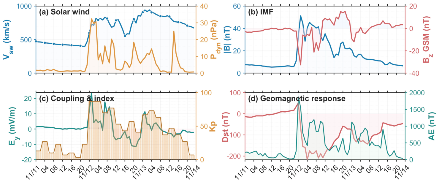
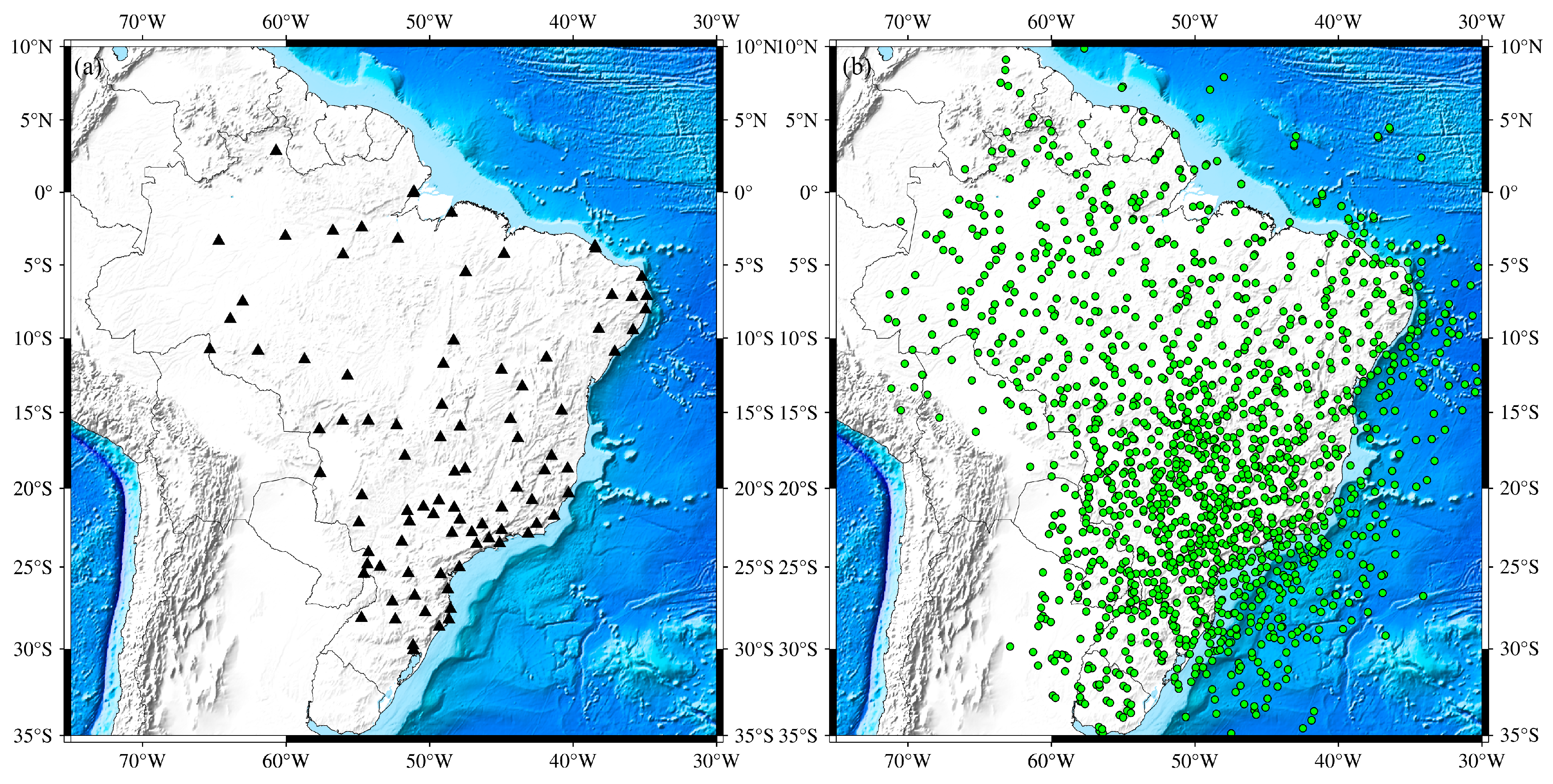
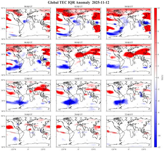
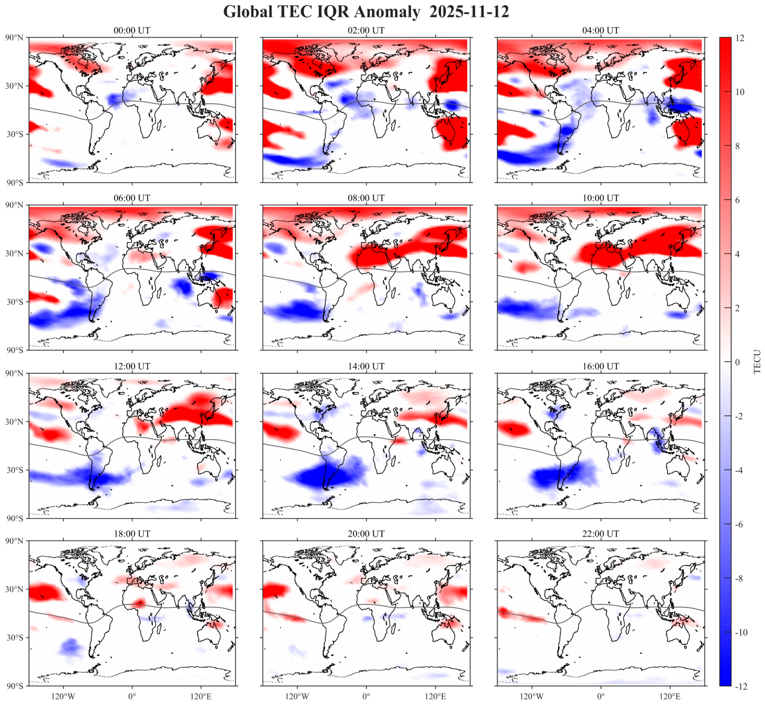
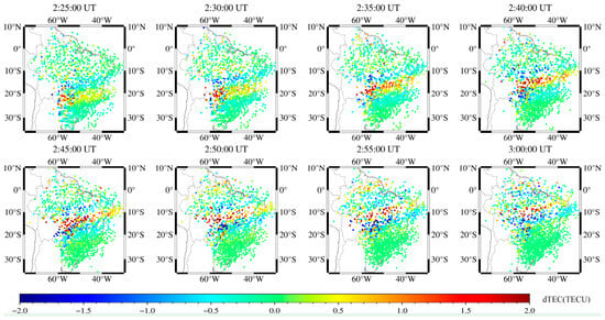
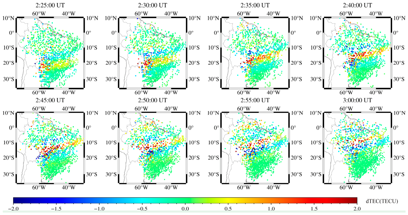
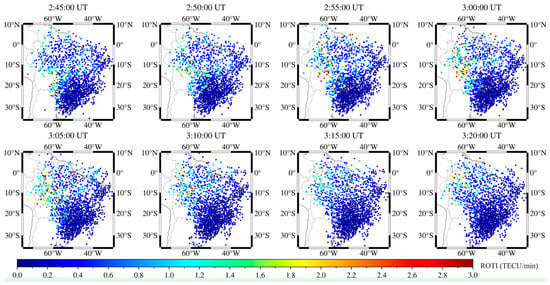
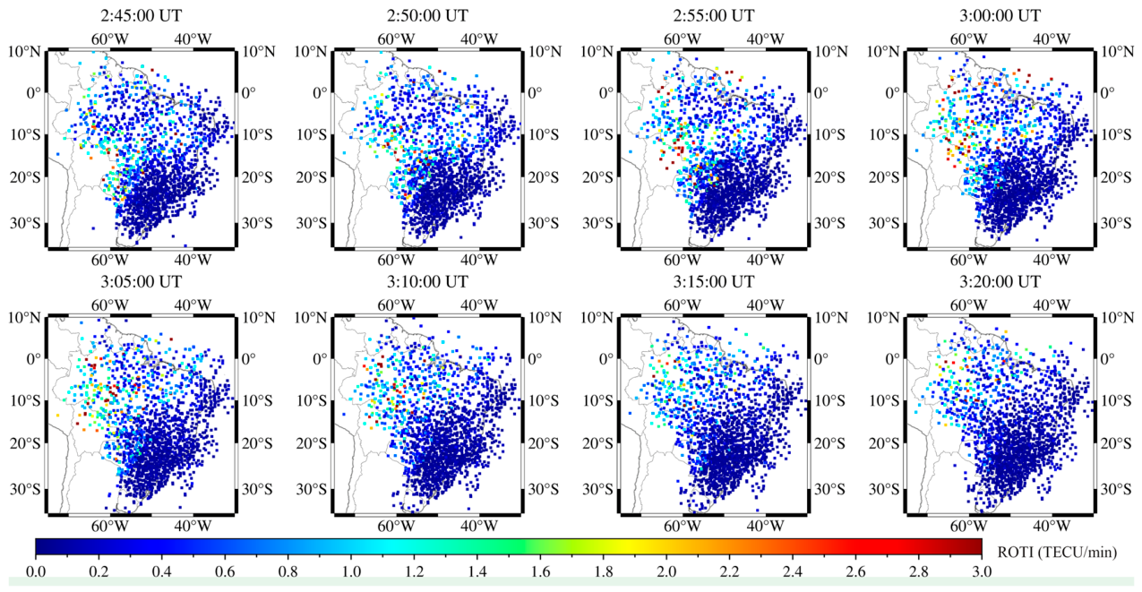
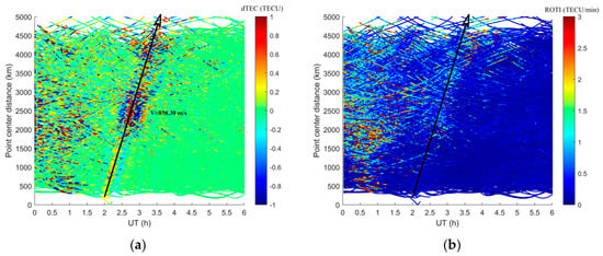
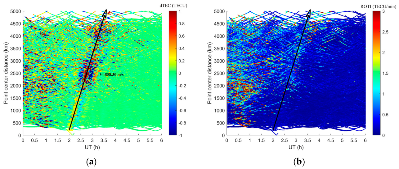
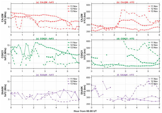
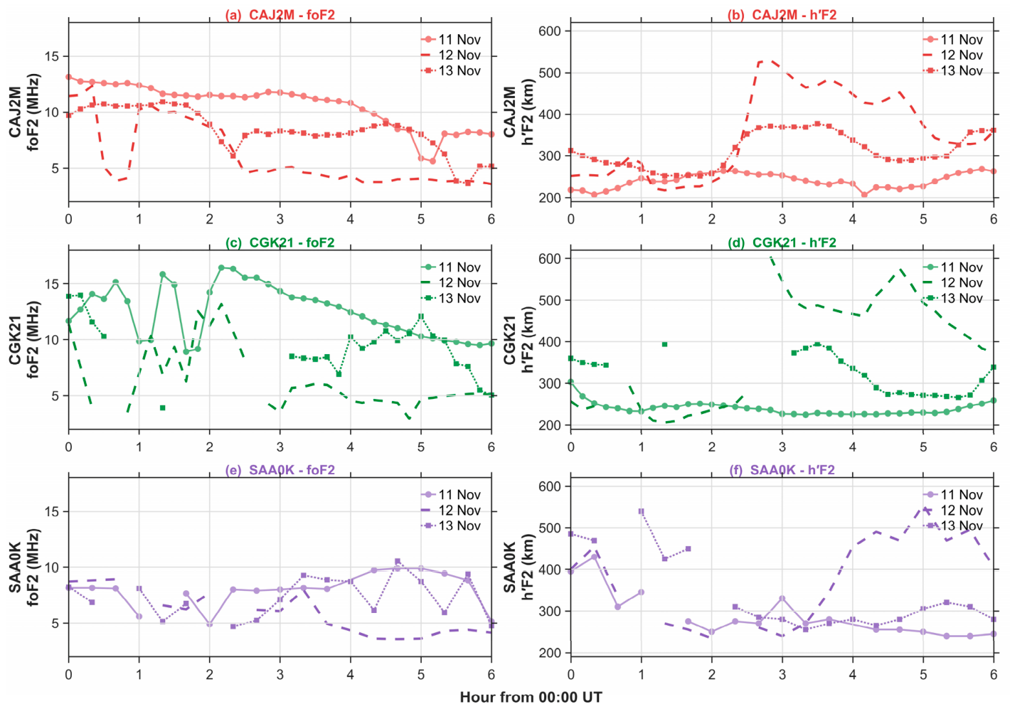
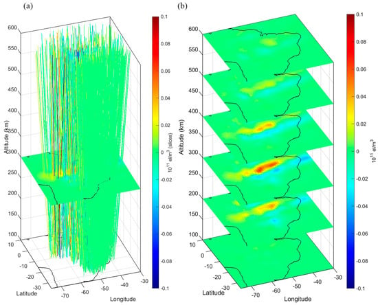
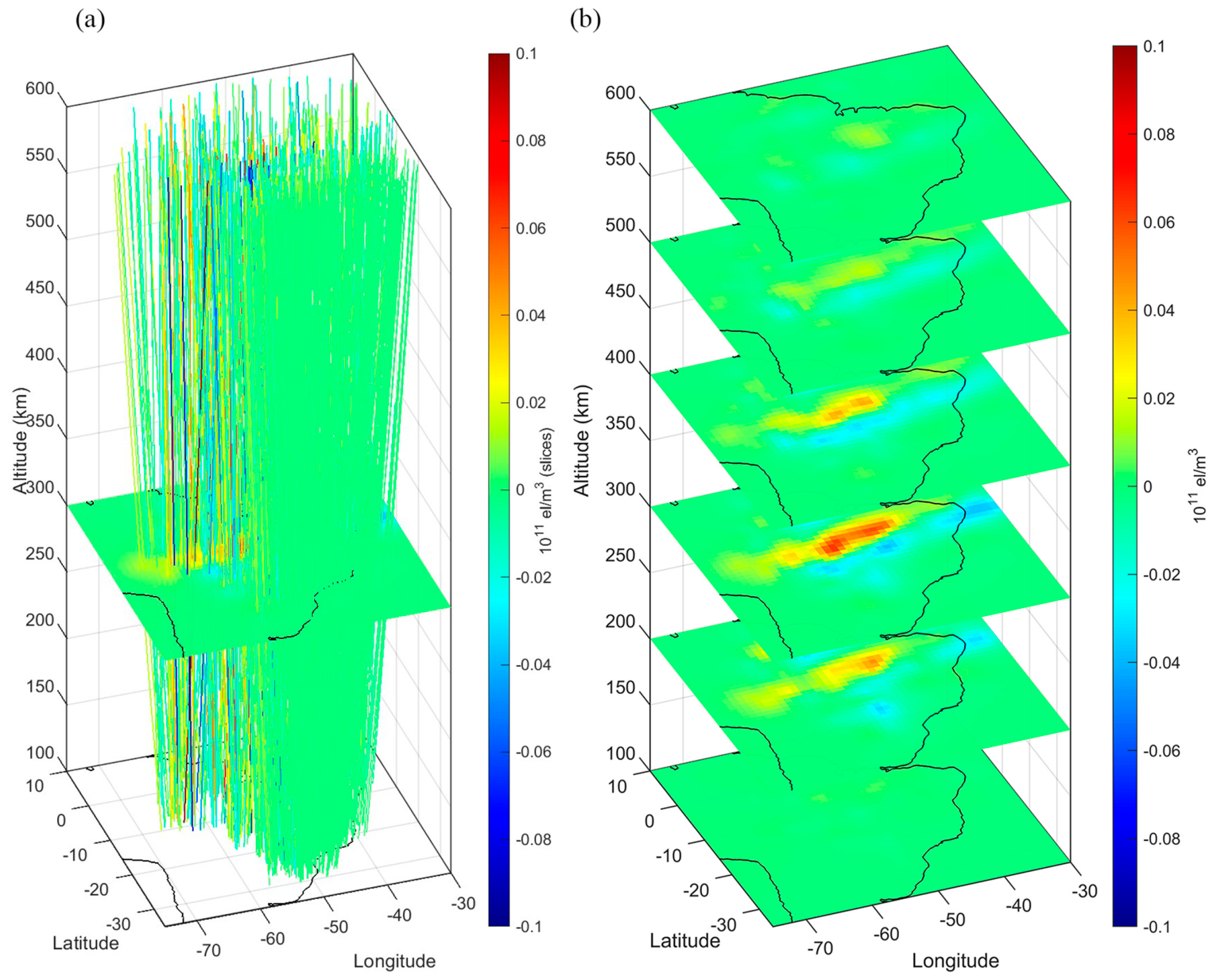
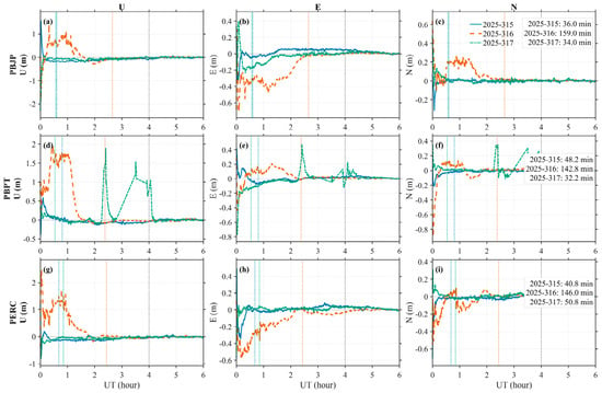
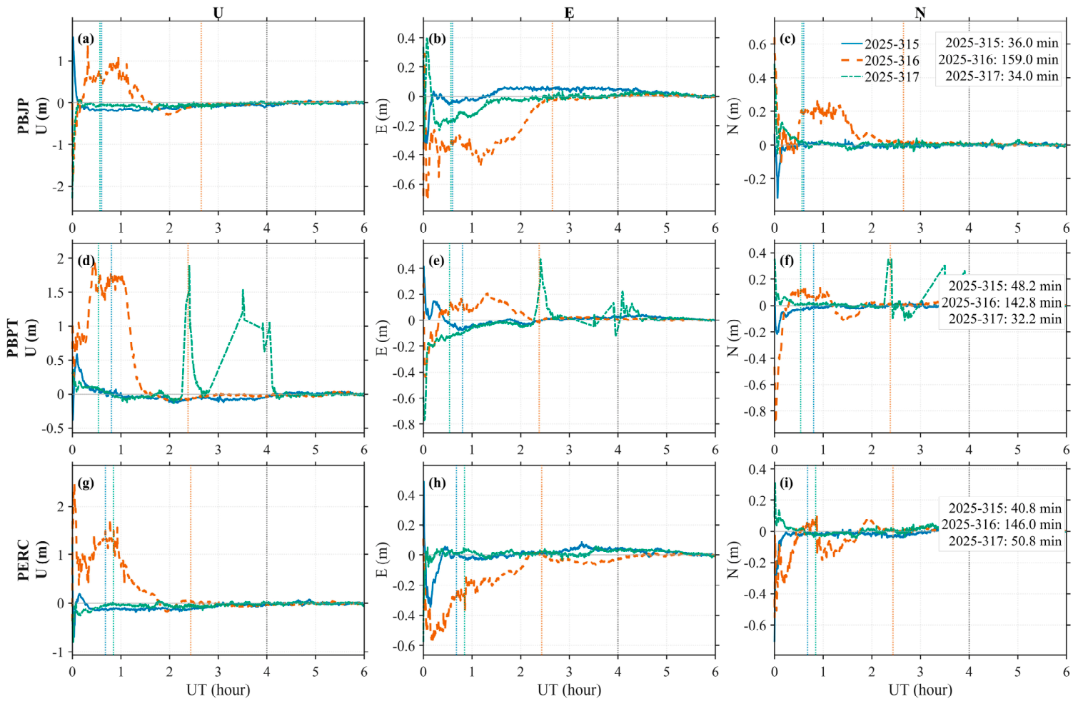
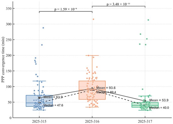
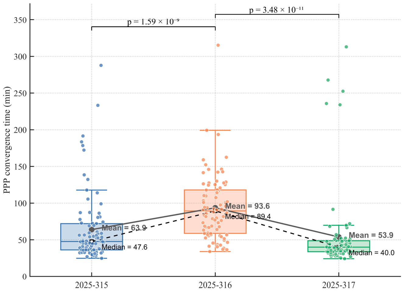

Disclaimer/Publisher’s Note: The statements, opinions and data contained in all publications are solely those of the individual author(s) and contributor(s) and not of MDPI and/or the editor(s). MDPI and/or the editor(s) disclaim responsibility for any injury to people or property resulting from any ideas, methods, instructions or products referred to in the content. |
© 2026 by the authors. Licensee MDPI, Basel, Switzerland. This article is an open access article distributed under the terms and conditions of the Creative Commons Attribution (CC BY) license.