Bayesian Spatial Partitioning with Feature Fusion for Wide-Beam SAR Altimeter Localization Using Delay-Doppler Maps

Highlights

What are the main findings?

• An XGBoost-based multi-feature fusion framework for DDM matching is presented, which adaptively integrates complementary similarity features to achieve robust single-frame matching and positioning, with matching accuracy improved by approximately 22 percentage points compared to optimal single-feature methods. Additionally, an adaptive sequential positioning method based on particle filtering is proposed, which employs a fast reference template generation method and adaptive sequential filtering to realize online generation and matching of dynamic spatial grids, eliminating the constraints of fixed search grids while achieving convergence within 10 frames across diverse motion scenarios.

What are the implications of the main findings?

• The proposed framework provides a high-precision autonomous positioning solution for airborne platforms in GNSS-denied environments, particularly under challenging conditions, including wide-beam configurations and high-altitude maneuvering flight.
• The ensemble learning approach achieves robust generalization with limited training data, facilitating practical engineering deployment. The dynamic grid mechanism addresses the specific positioning demands of aperture-constrained maneuvering platforms operating under wide-beam conditions, where conventional fixed-grid TAN suffers from boundary truncation and elevation measurement degradation induced by large footprint deviations.

Abstract

Terrain-aided navigation (TAN) enables autonomous positioning through fusing prior terrain databases with real-time sensor measurements in GNSS-denied environments. Typical factors, including wide beam width and terrain elevation variations, introduce inaccuracies in elevation measurements, degrading the performance of classical elevation-based TAN methods. The SAR altimeter operates in nadir-looking mode to acquire range–Doppler projection images with inherent cross-track ambiguity for positioning based on image information, yet its accuracy is limited by single-feature and fixed-grid approaches. In this paper, we introduce an adaptive positioning framework for the SAR altimeter that combines XGBoost-based multi-feature fusion with Bayesian particle filtering. First, a fast DDM template generation algorithm is employed to improve computational efficiency. Then, an ensemble learning framework integrating complementary similarity features is introduced to achieve robust single-frame matching. Additionally, a Bayesian filtering-based dynamic grid construction method is developed to concentrate particles in high-probability regions, eliminating boundary truncation errors inherent to fixed approaches. The proposed method’s primary advantage is the reliable three-dimensional localization under extreme radar configurations, such as wide beam width and high-altitude maneuvering platforms. Experimental results based on both simulated and real data validate the method, demonstrating superior positioning performance under wide-beam conditions.

1. Introduction

Applying radar altimeters to airborne platform positioning is an effective geophysical positioning technology. Radar altimeters have evolved from primitive one-dimensional ranging devices into sophisticated sensors capable of acquiring high-resolution terrain information. These systems have become indispensable for topographic measurement, playing a vital role in applications ranging from oceanography to terrestrial mapping [1,2,3]. Unlike optical sensors, which are susceptible to weather and lighting conditions, radar altimeters operate on the principle of active microwave transmission and reception, thereby enabling all-weather, day–night operational capability. This characteristic, combined with their ability to provide direct measurements of terrain elevation, has established radar altimeters as critical components in modern navigation systems—particularly in scenarios where Global Navigation Satellite Systems (GNSSs) are unavailable, jammed, or degraded [4,5,6].

The integration of radar altimeters into Terrain-Aided Navigation (TAN) systems represents a significant advancement in autonomous positioning technology for GNSS-denied environments. TAN estimates spatial position by fusing a priori terrain reference databases with real-time sensor measurements [7]. Conventional TAN approaches primarily rely on one-dimensional terrain elevation profiles, with two classical algorithms typifying this paradigm: Terrain Contour Matching (TERCOM), which correlates measured elevation sequences with pre-stored Digital Elevation Model (DEM) profiles, and Sandia Inertial Terrain-Aided Navigation (SITAN), which fuses INS data with radar altimeter measurements through an Extended Kalman Filter (EKF) framework [8,9]. However, these methods are fundamentally constrained by their reliance on one-dimensional elevation information, rendering them susceptible to multi-peak ambiguity in flat areas, leading to the invalidity of local linearization assumptions and further significant positioning errors in areas with severe terrain undulations [10,11,12]. Furthermore, practical constraints often necessitate wide beamwidth operation, either due to application requirements or platform limitations. Wide beamwidth causes the closest surface point to deviate from the nadir point when surface roughness is relative to aircraft altitude, resulting in inaccurate elevation measurements that further degrade positioning accuracy [13]. These limitations necessitate the exploration of alternative approaches leveraging richer terrain information.

The development of Synthetic Aperture Radar (SAR) technology has made high-resolution imaging of terrain assisted positioning possible. Early methods focused on side view SAR systems, which used optical matching algorithms [14] or deep learning methods [15,16,17] to match real-time SAR images with reference images. While demonstrating promising results, these methods typically impose strict constraints on the flight dynamics of the platform [18] and face generalization challenges with limited training data [19]. Additionally, SAR images are often affected by speckle noise, and the matching effect of SAR images using optical matching algorithms is relatively poor. Currently, most research on SAR-based positioning focuses on side-looking SAR systems, while nadir-looking SAR altimeter positioning based on two-dimensional DDM image matching remains relatively underexplored compared to conventional POCA-based ranging approaches.

The advent of the Synthetic Aperture Radar Altimeter (SAR altimeter) marks a significant technological convergence, effectively bridging the gap between traditional altimetry and imaging radar capabilities [20]. By applying synthetic aperture technology to altimeters, the SAR altimeter overcomes the resolution limitations inherent in traditional radar altimeters. Within the beam observation range, the SAR altimeter enables the fine-grained processing of backscattered signals, extracting rich two-dimensional scattering features and thereby allowing for the accurate inversion of ground elevation data [21]. Unlike side-looking SAR, which achieves lateral high resolution via azimuth synthetic aperture, the SAR altimeter operates in a nadir-looking observation mode. It enhances along-track resolution through Delay-Doppler processing, establishing a unique two-dimensional observation space defined by the range–Doppler domain. This configuration facilitates the generation of Delay-Doppler Maps (DDMs), which encode comprehensive terrain characteristics within the radar footprint while maintaining a compact system architecture suitable for airborne deployment.

In recent years, three-dimensional positioning technology based on two-dimensional SAR altimeter DDM images has gradually emerged as a promising approach for terrain-aided navigation. Unlike traditional altimeters that solely rely on single-point elevation measurements for terrain-aided positioning, DDM-based methods exploit the rich two-dimensional scattering information inherent in nadir-looking imagery to achieve robust localization. For instance, Wei et al. [22] presented a hybrid three-dimensional positioning framework that combines DDM Phase Correlation (PC) matching with spatio-temporal echo similarity, demonstrating high-precision positioning capability with enhanced terrain adaptability and robustness. Lu et al. [23] developed a model-driven neural network algorithm named “TMP-Net” that acquires terrain DDMs via an SAR altimeter and employs a presented three-point weighted positioning scheme to match with reference maps generated from DEM data. The core principle underlying these methods involves dynamically comparing real-time radar altimeter nadir-looking DDMs with a bank of candidate reference images utilizing various similarity metrics to inversely solve for spatial position. Leveraging the richer ground information embedded in nadir-looking DDMs, these approaches have significantly improved the accuracy and reliability of TAN, particularly in complex terrain and wide-beam scenarios.

However, despite the demonstrated potential of DDMs for three-dimensional localization, two interrelated challenges persist, hindering further performance enhancement. First, the inherent low-dimensional and potential aliased nature of nadir-looking DDMs [22] renders similarity metrics highly sensitive to the specific choice of feature extraction and comparison algorithms. The complexity and diversity of terrain features often induces instability in single-feature matching, while deep learning approaches face generalization challenges despite their strong performance capabilities. Second, current DDM-based positioning methods predominantly rely on pre-computed, fixed search grids that are defined a priori based on approximate position estimates. This approach fundamentally restricts real-time adaptability to unpredicted platform maneuvers and imposes unnecessary computational loads on irrelevant search regions. When an aircraft deviates from preset trajectories due to tactical requirements or environmental factors, fixed-grid methods may fail to converge or produce significant positioning errors due to boundary truncation effects.

In this paper, an adaptive positioning framework integrating XGBoost-based multi-feature fusion with Bayesian particle filtering is proposed for the SAR altimeter. First, to enhance computational efficiency, a fast DDM template generation algorithm is introduced. Then, an ensemble learning framework integrating complementary similarity features is developed to achieve robust single-frame matching. Additionally, to address the limitations of fixed search grids, a particle-filtering-based dynamic grid construction method is employed, effectively concentrating particles within high-probability regions and thereby mitigating boundary truncation errors. Comprehensive experimental validation using both simulated and real SAR altimeter data is conducted, demonstrating superior positioning performance under wide-beam conditions.

The main contributions of this work are as follows:

• An XGBoost-based multi-feature fusion framework for DDM matching is introduced. This approach adaptively integrates complementary similarity features to achieve robust single-frame matching and positioning.
• An adaptive sequential positioning method based on Bayesian filtering is developed to address the severe boundary truncation errors inherent to wide-beam footprints. By employing a fast reference template generation method and adaptive sequential filtering, this method enables the online generation and matching of dynamic spatial grids, thereby eliminating the constraints imposed by fixed search grids.
• Comprehensive experimental validation using both simulated and real SAR altimeter data is conducted, demonstrating the superiority and robustness of the proposed approach compared with existing methods under wide-beam conditions.

2. Airborne SAR Altimeter: Geometric and Signal Models

This section introduces the theoretical foundation for the airborne SAR altimeter. By integrating nadir-looking observation geometry with Delay-Doppler processing, the SAR altimeter synthesizes two-dimensional Delay-Doppler Maps (DDMs) that encode detailed terrain information. The geometric observation and signal transmission models detailed herein constitute the fundamental basis for subsequent DDM generation and terrain matching algorithms.

2.1. Geometric Observation Model

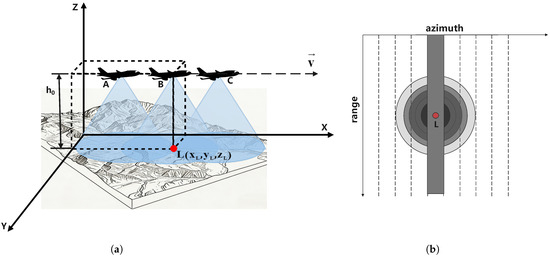
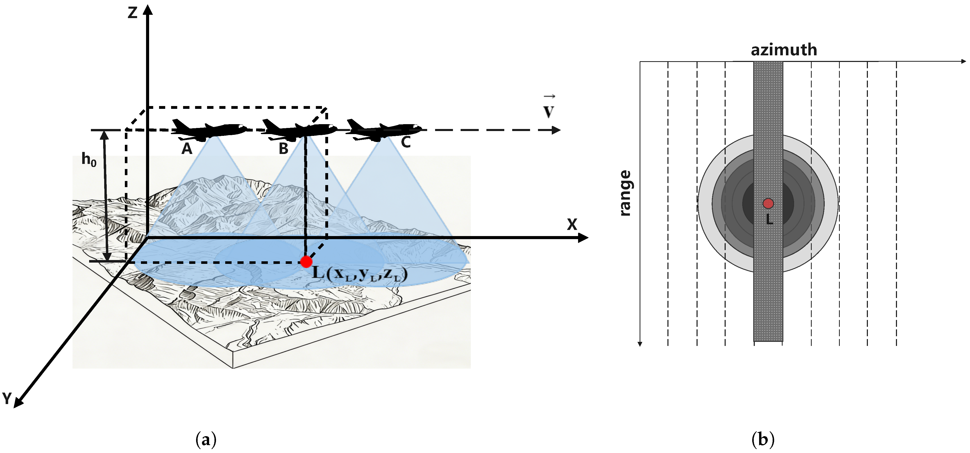
To accurately describe the spatial relationships between the SAR altimeter platform and ground scatterers, we establish a three-dimensional Cartesian coordinate system as shown in Figure 1a. This coordinate system provides a convenient framework for analyzing the kinematics and signal propagation characteristics inherent to the nadir-looking geometry. We consider an airborne SAR altimeter platform moving at a constant velocity $\overrightarrow{v}$ along the positive X-direction at a nominal altitude $h_0$ above the reference plane. The platform position at time t is denoted as $P\left(t\right)=\left(vt,0,h_0\right)$.

Figure 1. Airborne SAR altimeter geometry: (a) the geometric model of airborne SAR altimeter. (b) Doppler pulse footprint.

For an arbitrary ground scatterer L located at coordinates $\left(x_L,y_L,z_L\right)$, where $z_L$ represents the elevation relative to the reference plane, the relative position vector from the platform to the scatterer is given by

$$r_{pL}=\left(x_L-vt,y_L,z_L-h_0\right).$$

(1)

The instantaneous slant range from the platform to scatterer L is $R\left(t\right)=∥r_{pL}∥$ ($\parallel$ $\parallel$ is the Euclidean norm). Of particular significance is the nadir observation condition, occurring when the radar platform travels directly over scatterer L. At this instance, $x_p=x_L$ and $y_p=y_L$, causing the horizontal projections of the radar and scatterer positions to coincide. Under nadir conditions, the slant range is the shortest [24].

The SAR altimeter antenna transmits a beam with finite angular width, typically quantified by the half-power beamwidth ${\theta }_{hp}$. This beam illuminates an elliptical footprint on the ground surface, as illustrated in Figure 1a. A key characteristic of nadir-looking geometry is that the beam coverage extends beyond the nadir point to include scatterers positioned both ahead of and behind the platform along the flight direction. Consequently, the received echo signal consists of superimposed backscattering contributions from multiple scatterers within the illuminated area, thereby providing the spatial diversity essential for two-dimensional imaging.

To overcome the inherent limitation of conventional radar altimeters, namely, poor azimuth resolution, the SAR altimeter incorporates Delay-Doppler processing [25]. The fundamental principle of Delay-Doppler processing exploits the differential Doppler frequency shifts induced by scatterers at distinct along-track positions. As the platform moves forward, scatterers ahead of the nadir point exhibit positive Doppler shifts, whereas those behind exhibit negative Doppler shifts. Through azimuthal signal processing, the wide beam is effectively divided into multiple narrow sub-beams, each corresponding to a specific Doppler frequency band.

As shown in Figure 1b, the beam illumination area forms a concentric circular footprint on the ground, subdivided into multiple azimuthal sub-regions by isodoppler lines. Each sub-region corresponds to a specific Doppler frequency band. By performing azimuthal Fourier transform on the echo signal, signal components within different Doppler frequency bands can be extracted, effectively simulating high-precision observation using multiple narrow beams. The resolution improvement multiple achieved via Delay-Doppler processing is proportional to the Doppler frequency band width, significantly improving the detection accuracy in the along-track direction without increasing the antenna size.

2.2. SAR Altimeter Signal Model

The SAR altimeter achieves imaging by transmitting Linear-Frequency-Modulated (LFM) signals [26] and receiving echoes from ground scatterers. Its echo signals contain two-dimensional information in the range direction (fast time) and azimuth direction (slow time):

$${\mathrm{s}}_t\left(\tau \right)=w_r\exp \left(j\pi K_r{\tau }^2\right),$$

(2)

where $\tau$ is the fast time (range-direction time variable), $w_r\left(\tau \right)$ is the range-direction window function (usually a rectangular window or Hanning window), and $K_r$ is the frequency modulation slope. This signal is modulated by the carrier frequency $f_0$ (with a corresponding wavelength of $\lambda$, where c is the speed of light) before transmission.

When the radar platform observes the ground scatterer L at the slow time $\eta$ (azimuth-direction time variable), the round-trip propagation distance of the signal is $R\left(\eta \right)$. At this time, the received echo signal can be expressed as

$$\begin{array}{cc}\hfill s_{pul}\left(\tau \right)=& A_0{w}_r\left\{\tau -{\displaystyle \frac{2R\left(\eta \right)}{c}}\right\}{w}_a\left(\eta -{\eta }_c\right)\hfill \\ & \times \cos \left\{2\pi f_0\left(\tau -{\displaystyle \frac{2R\left(\eta \right)}{c}}\right)+\pi K_r{\left(\tau -{\displaystyle \frac{2R\left(\eta \right)}{c}}\right)}^2+\psi \right\},\hfill \end{array}$$

(3)

where $A_0$ is the constant related to the backscattering coefficient of the scatterer, $w_a\left(\eta -{\eta }_c\right)$ is the azimuth-direction window function (with ${\eta }_c$ being the azimuthal center time), and $\psi$ is the phase change introduced by the scattering process.

By performing operations such as de-slope compression, matched filtering, and slow-time processing on the original echo signal [27], the signal expression can be obtained as

$$s_r\left(\tau ,\eta \right)=w_r\left\{\tau -{\displaystyle \frac{2R\left(\eta \right)}{c}}\right\}{W}_a\left(f_{\eta }-f_{{\eta }_c}\right)·\exp \left\{-j{\displaystyle \frac{4\pi f_0{R}_0}{c}}\right\}\exp \left\{-j\pi {\displaystyle \frac{f_{\eta }^2}{K_a}}\right\},$$

(4)

where $W_a$ is the frequency-domain form of the azimuth-direction window function and $f_{\eta }$ is Doppler frequency.

The azimuth resolution is determined by the Doppler bandwidth, with a larger bandwidth yielding a higher resolution. Its theoretical value is $\lambda h_0/\left(2v{L}_a\right)$(where $L_a$ is the synthetic aperture length). The instantaneous distance $R\left(\eta \right)$ is a key parameter describing the echo characteristics, and its expression is

$$R\left(\eta \right)=\sqrt{R_0^2+v^2{\eta }^2}\approx R_0+{\displaystyle \frac{v^2{\eta }^2}{2R_0}},$$

(5)

where $R_0$ is the minimum slant range. The corresponding Doppler frequency is approximately

$$f_d\left(\eta \right)\approx -\left(2v^2/\lambda R_0\right)\eta .$$

(6)

This linear relationship between Doppler frequency and azimuth time enables the formation of the two-dimensional Delay-Doppler Map through coherent integration over the azimuth observation window. The final DDM is generated by organizing the processed echo signals into a two-dimensional matrix, where the horizontal axis represents range (or equivalently, delay) and the vertical axis represents Doppler frequency. Mathematically, the DDM intensity at range gate m and Doppler bin n is given by

$$DDM\left[m,n\right]={\left|\int s_r({\tau }_m,\eta )\exp \left[-j2\pi f_n\eta \right]d\eta \right|}^2,$$

(7)

where ${\tau }_m$ corresponds to the m-th range gate and $f_n$ corresponds to the n-th Doppler frequency.

The range dimension of the DDM corresponds to the slant range from ground scatterers to the radar platform. This dimension is directly related to terrain elevation: for a given platform altitude, scatterers at higher elevation yield shorter slant ranges and thus appear at lower range gate indices. The range resolution $p_r$ is determined by the signal bandwidth B: $p_r=c/\left(2B\right)$.

In traditional SAR imaging, methods such as range migration correction can be used to obtain spatially undistorted focused images. However, considering the azimuth aliasing characteristics of nadir-looking radar images, range migration correction cannot completely decouple the influence of platform motion and does not provide additional terrain information. Therefore, in this paper, uncorrected DDM images are used for terrain matching processing to improve computational efficiency.

Due to the nadir-looking observation geometry, scatterers symmetric about the nadir point are mapped to the same range–Doppler bins, resulting in inherent forward–backward Doppler symmetry. Meanwhile, cross-track position information is aliased into the DDM through the range dimension, making cross-track features poorly observable but strongly coupled to the image structure. These properties lead to high inter-frame similarity and necessitate refined feature extraction algorithms to capture subtle cross-track variations essential for terrain matching.

3. Methodology

This section presents the proposed methodology for DDM-based terrain matching and positioning. The framework addresses the unique challenges identified in Section 2 through three synergistic components: (1) a multi-feature fusion strategy based on XGBoost ensemble learning for robust single-frame matching; (2) a fast reference template generation method for efficient DDM computation; and (3) an adaptive particle filtering framework that constructs dynamic reference matching grids for sequential Bayesian positioning.

3.1. Overall Framework

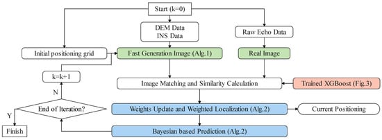
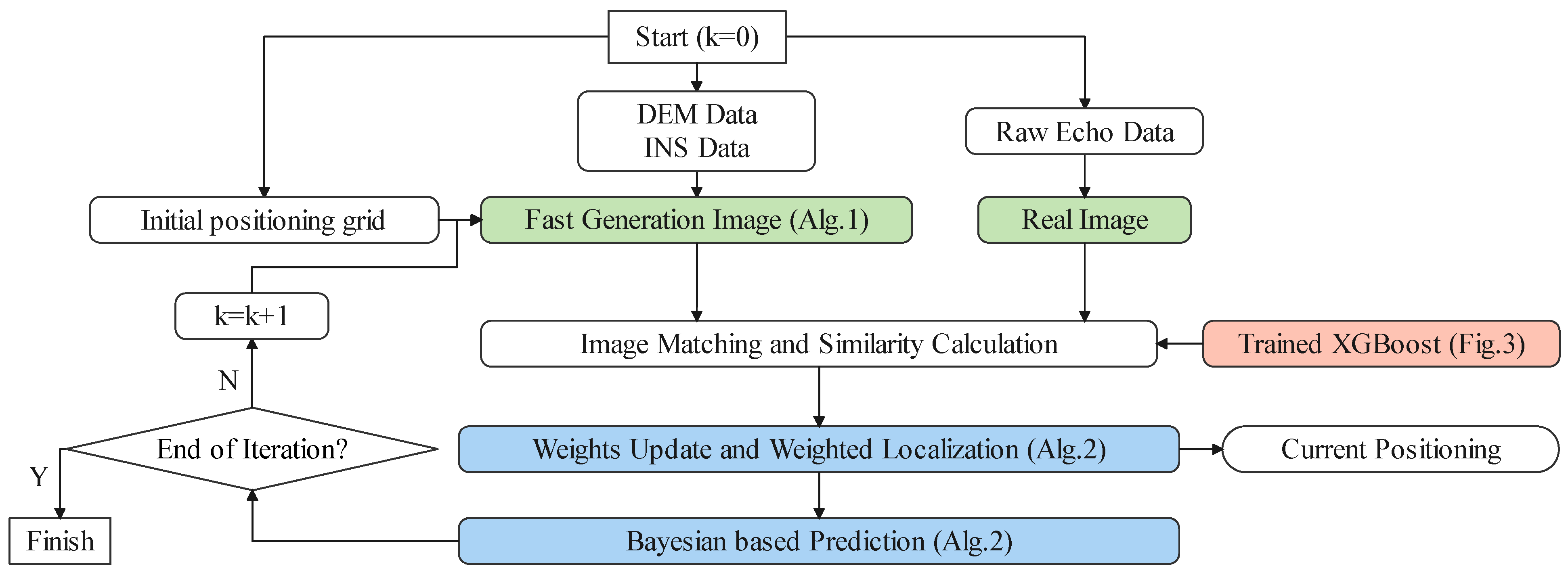
The proposed matching and positioning framework is based on real-time radar echo processing, integrating reference database management with dynamic state estimation to achieve full-process closed-loop optimization from raw signal to final three-dimensional position estimates. As illustrated in Figure 2, the framework comprises five interconnected modules.

Figure 2. The flowchart of the introduced matching and positioning algorithm.

Module 1: Data Preprocessing and Initialization. This module reads the initial three-dimensional position and flight state information from the Inertial Measurement Unit (IMU) at time k = 0, initializes the positioning grid, and loads the system state model. It synchronously ingests raw radar echo data and pre-stored reference DEM data and then generates the measured DDM from the radar signal using the signal model introduced in Section 2.2.

Module 2: Reference DDM Generation. For each particle within the matching grid (detailed in Section 3.4), this module generates a simulated reference DDM on-the-fly via the efficient DDM generation algorithm introduced in Section 3.3. The generated reference DDMs serve as templates for subsequent similarity comparison with the real-time observation.

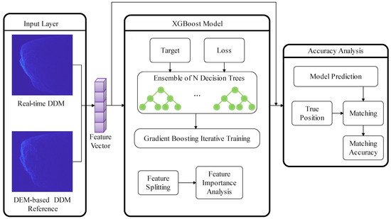
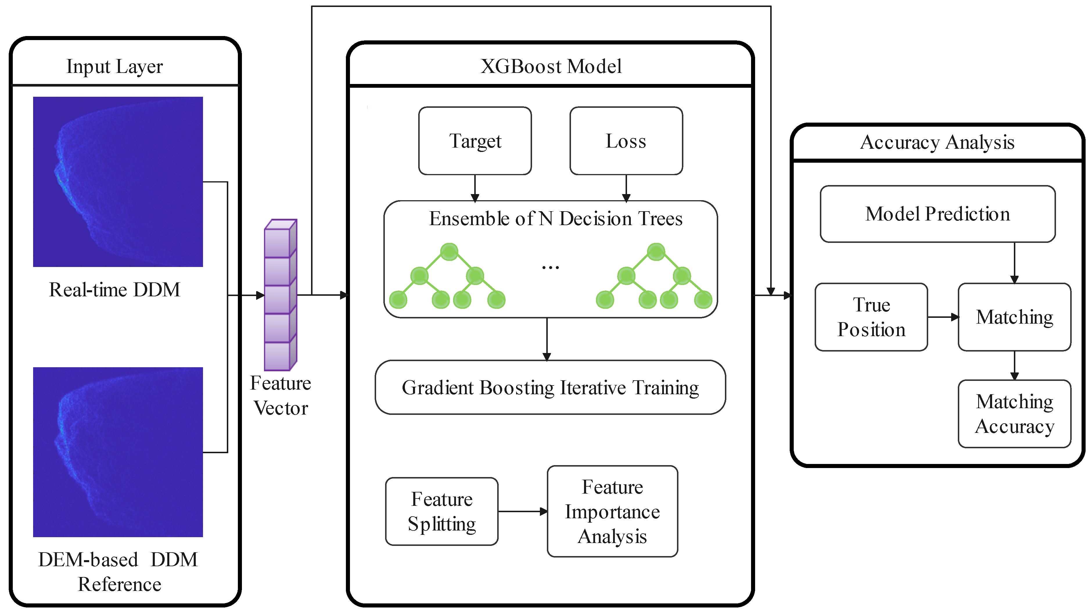
Module 3: Similarity Calculation. Serving as the framework’s core, this module executes a combined feature measurement strategy based on the XGBoost algorithm as shown in Figure 3. It quantifies the spatial correlation between the measured DDM and each reference DDM by extracting and fusing multiple complementary feature types, as detailed in Section 3.2.

Figure 3. The algorithm block diagram of XGBoost model.

Module 4: Bayesian Estimation and Weighted Positioning. This module dynamically adjusts the particle distribution of the reference matching grid according to the Bayesian filtering framework. Particle weights are updated based on the similarity-likelihood implicit model, and state focusing is achieved through resampling. The final position estimate for the current frame is output through weighted averaging of particle states.

Module 5: Adaptive Grid Management. Operating synergistically with the Bayesian filtering concept, this module dynamically generates the matching point grid by fusing particle filter predictions with the SAR altimeter motion state model. This adaptive approach ensures an efficient concentration of particles within high-probability regions, as discussed in Section 3.4.

The framework operates iteratively, with the output position estimate at time k serving as the prior information for particle prediction at time k + 1, thereby forming a continuous positioning loop that exploits spatio-temporal correlations.

3.2. Single DDM Matching Method Based on Combined Features

Image similarity measurement realizes the spatial solution of matching positioning by quantifying differences in pixel distribution, structural features, and gradient characteristics between real-time images and reference images [28]. Due to the complexity of terrain, it is challenging to analytically determine the optimal feature similarity metric for DDM image matching from a mathematical perspective. Generally, DDM images have unique characteristics, such as strong speckle noise, low contrast, and observation aliasing under nadir geometry, making it difficult for a single similarity measurement method to fully characterize the spatial correlation between images. For example, ORB [29] suffers from insufficient matching points in low-feature areas, while single-scale SSIM [30] cannot balance macro contours and micro details. Given these limitations, we posit that a robust matching criterion can be constructed through multi-feature fusion. Traditional manual weighted fusion methods, however, struggle to handle the nonlinear redundant relationships that exist between features [31]. For instance, grayscale-based NCorr2 and structure-based MS-SSIM encode overlapping information regarding macro terrain contours, and simple linear combination cannot adaptively balance their contributions across diverse terrain types. Thus, we introduce an XGBoost-based adaptive similarity learning framework that achieves strong generalization with few training samples while maintaining computational efficiency for online operation.

XGBoost is an ensemble learning algorithm based on Gradient Boosting Decision Trees (GBDTs) [32]. Its training strategy follows the boosting paradigm in ensemble learning: multiple “weak learners” (simple decision trees) [33] are sequentially trained, with each new learner focusing on correcting the errors of the existing ensemble. The final model combines all weak learners through weighted voting to form a powerful predictor. Mathematically, given a training set $\left\{\left(x_i,y_i\right)\right\}$, where $x_i$ represents the feature vector and $y_i$ represents the target label, XGBoost minimizes the following regularized objective:

$$L\left(\theta \right)={\sum }_{\theta }\mathrm{l}\left({y_i,\widehat{y}}_i\right)+{\sum }_k\Omega \left(f_k\right),$$

(8)

where l is a differentiable convex loss function, $\Omega$ penalizes model complexity, and $f_k$ represents the prediction of the k-th tree.

Based on the physical characteristics of DDM images, we select five types of similarity features: statistical correlation, structural, point-based, line-based, and gradient features, which together constitute the input feature vector. The local correlation coefficient (NCorr2) [34] is selected for statistical correlation features; Multi-Scale Structural Similarity (MS-SSIM) [35] for structural features; the ORB feature point detection for point features; the HoughLineP algorithm [36] for line features; and the Histogram of Oriented Gradients (HOG) [37] for gradient features. The core principles, adaptability, and limitations of each type of feature are summarized in Table 1.

Table 1. Characteristics of DDM matching methods.

Method	Core Principle	Advantages	Limitations
NCorr2	Sliding-window local correlation	Sensitive to local features	High computational complexity
MS-SSIM	Multi-scale structural similarity	Balances multi-scale information	High computational complexity
ORB	FAST detection + BRIEF descriptor	Fast, rotation-invariant	Insufficient feature points
HoughLineP	Hough transform line detection	Robust to edge breakage	Limited valid lines
HOG	Cell-based gradient orientation	Strong texture discrimination	Weak features in smooth terrain

For the training label of the XGBoost model in this experiment, it is necessary to establish a quantitative mapping relationship between “feature similarity” and “spatial position correlation”. Based on the spatial positioning requirements of DDM matching, we introduce a target value constructed based on Euclidean distance to quantify the spatial similarity between the reference point and the real track:

$$target={\left(1-\sqrt{{\displaystyle \frac{r}{R_{\max }}}}\right)}^2,$$

(9)

where r is the 3D Euclidean distance between the reference point and the real position of the track and $R_{\max }$ is the maximum search distance (set to 300 m in the experiment), which can cover most of the initial positioning error range. The squared form ${(1-\sqrt{r/R_{\max }})}^2$ serves two purposes: it ensures that the target value decreases monotonically as the spatial deviation increases, and that the square root operation compresses the dynamic range, preventing small distance variations from causing drastic target changes. This design facilitates smoother optimization during gradient boosting and aligns with the similarity-likelihood mapping required for particle weight updates in Section 3.4.

The input of the training model is the five-dimensional feature vector described in Table 1, and the output is the predicted similarity value. To train the XGBoost regression model, we construct a training set that comprehensively covers the spatial search space. For each true trajectory point, we generate reference points by sampling uniformly within the search radius $R_{\max }=300 \mathrm{m}$. This sampling strategy ensures the inclusion of both proximal samples and distal samples, enabling the model to learn the full spectrum of the similarity–distance relationship. The target value is computed using Equation (9).

The hyperparameters in Table 2 were determined through a combination of domain knowledge and systematic cross-validation. We performed a grid search over learning rate $\eta \in \{0.05,0.1,0.2,0.3\}$, maximum depth $\in \{4,5,6,7,8\}$, and regularization coefficient $\lambda \in \{0.5,1.0,2.0\}$. The combination $(\eta =0.2,\mathrm{depth}=6,\lambda =1.0)$ achieved the highest 5-fold cross-validation accuracy [38]. The 1000-iteration limit was determined through early stopping analysis, where validation accuracy plateaued after approximately 800–900 iterations across all folds. Beyond 5-fold cross-validation, we adopt three complementary regularization mechanisms: L2 regularization ($\lambda =1$), early stopping with a patience of 50 rounds, and a maximum tree depth of 6. Together, these strategies effectively prevent overfitting and promote reliable generalization to unseen terrain data.

Table 2. Core parameters of XGBoost model.

Parameter	Value	Function
Learning Rate ($\eta$)	0.2	Controls the weight contribution of each tree
Maximum Tree Depth	6	Limits the complexity of decision trees
Number of Leaf Nodes	64	Prevents insufficient samples in leaf nodes
Regularization Coefficient ($\lambda$)	1	Constrains the sum of squares of tree weights
Number of Iterations	1000	Number of decision trees

During training, a gradient boosting strategy of “iterating tree by tree” is adopted. Initially, one decision tree is constructed to fit the target values; each subsequent tree aims to minimize the residual (difference between predicted and target values) of the previous model. Feature selection at each split is optimized via gradient descent, and the importance of input features is ranked based on the split gain metric.

Subsequently, the model results of the test set are evaluated. The core indicator is the matching accuracy, i.e., the proportion of reference points with the highest predicted similarity where the Euclidean distance to the real position is less than the threshold. The calculation logic for determining whether the i-th sample matches accurately is

$$I_i=\left\{\begin{array}{cc}\hfill & 1,\mathrm{if}{r}_i\le \gamma \hfill \\ \hfill & 0,\mathrm{if}{r}_i>\gamma \hfill \end{array}\right.,$$

(10)

where $I_i$ is the indicator function and $r_i$ is the three-dimensional Euclidean distance between the reference point with the highest prediction similarity of the i-th test sample and the true position. Then, 5-fold cross-validation is used, and the average accuracy of each method is obtained by calculating the accuracy of each fold and taking the average.

3.3. Fast Reference Template Generation Method

The generation efficiency of DDM templates directly determines the real-time performance. In the subsequent adaptive grid algorithm, the particle filter needs to dynamically generate corresponding reference DDMs for hundreds of particles per frame. If the traditional finite element echo generation method is adopted, its complex signal processing workflow may lead to computational delays exceeding the tolerance range of the airborne platform. To address this, we introduce a fast reference DDM template generation method.

In Section 2.2, we mentioned the range–elevation mapping relationship: the range gate of the DDM is directly related to the slant range from the ground scatterer to the radar, and this mapping relationship can be directly established through simple geometric calculations. Meanwhile, the Doppler channel corresponds one-to-one with the along-track position of the scatterer, which can be calculated via speed and angle without FFT. For the backscattering coefficient of ground objects ${\sigma }_0$, it can be directly calculated through an empirical model. Based on the above theory, the fast method generates the reference DDM mainly through three steps: “geometric mapping, scattering coefficient calculation, power superposition”. The workflow comparison between this method and the traditional method is shown in Table 3.

Table 3. Comparison of flow between traditional finite element method and fast method.

Workflow Step	Traditional Finite Element Method	Fast Method
Signal Simulation	Generates and modulates LFM signal	Direct geometric mapping
Echo Calculation	Computes complex echoes per scatterer	Direct power contribution calculation
Range Compression	Matched filtering for de-chirping	Direct slant-range to range-gate mapping
Azimuth Processing	Azimuth FFT for Doppler analysis frequency shift	Direct speed/angle to Doppler mapping
Backscattering Model	Electromagnetic scattering equation	Empirical model

The specific workflow of fast DDM template generation is described in Algorithm 1. We assume that the number of range gates in the DDM image is M, the number of Doppler channels is N, and the number of discrete ground scatterers in the traditional finite element method is K. The computational complexity of the traditional finite-element method primarily arises from echo calculation, range compression, and azimuthal FFT, with complexities of $O\left(KMN\right)$, $O\left(M^{2}N\right)$, and $O\left(MN\log \left(N\right)\right)$, respectively. However, the fast reference template generation method introduced in this paper skips the above high-complexity steps. Its core workflow is geometric mapping → empirical scattering coefficient calculation → power superposition, and the computational burden of these steps is linear with respect to $O\left(KMN\right)$, with no high-order terms, resulting in a significant reduction in computational complexity. K is bounded by the ratio of the radar beam footprint area to the DEM cell area. For a given system configuration with fixed beamwidth and platform altitude, the footprint area remains constant, and K is therefore a bounded parameter.

3.4. Adaptive Reference Matching Grid Based on Particle Filtering

While single-frame matching identifies candidate positions, it does not exploit spatio-temporal continuity or adapt to dynamic maneuvering. This subsection introduces an adaptive positioning framework integrating Bayesian filtering with the matching algorithm, where particle filtering constructs a dynamic reference matching grid for autonomous three-dimensional positioning.

Algorithm 1 Fast DDM generation algorithm.

Input: Wavelength, $\lambda$; sensor position, $l_1\in {\mathbb{R}}^{3\times 1}$; sensor velocity, $v\in {\mathbb{R}}^{3\times 1}$; scatterer positions, $l_2\in {\mathbb{R}}^{K\times 3}$; DEM gradients, $g_x,g_y\in {\mathbb{R}}^{K\times 1}$; reference area, $A_0$; distance range, $r_x\in {\mathbb{R}}^{M\times 1}$; Doppler range, $f_D\in {\mathbb{R}}^{N\times 1}$.

1: Step-0. Basic calculation:

2: $d={∥l_1-l_2^T∥}_2$; $\overline{r}={\displaystyle \frac{l_1-l_2^T}{d}}$; $v_r=v^T·{\overline{r}}^T$; $f_d=-{\displaystyle \frac{2v_r}{\lambda }}$;

3: Step-1. Target screening:

4: $i_{d0}=\left\{n|d\left(n\right)\in r_x\cap f_d\left(n\right)\in f_D\right\}$; ${\overline{r}}^{\prime }=\overline{r}\left(i_{d0},:\right)$; $d^{\prime }=d\left(i_{d0},:\right)$; ${f_d}^{\prime }=f_d\left(i_{d0},:\right)$; $g_x^{\prime }=g_x\left(i_{d0}\right)$; $g_y^{\prime }=g_y\left(i_{d0}\right)$;

5: Step-2. Terrain slope correction:

6: $\mathbf{n}={\displaystyle \frac{(-g_x^{\prime },-g_y^{\prime },\mathbf{1})}{\sqrt{g_x^{\prime 2}+g_y^{\prime 2}+\mathbf{1}}}}$; ${\theta }_{local}=\arccos \left(\right|{\overline{r}}^{\prime }·\mathbf{n}\left|\right)$; $\alpha =\arcsin {\displaystyle \frac{\sqrt{g_x^{\prime 2}+g_y^{\prime 2}}}{\sqrt{g_x^{\prime 2}+g_y^{\prime 2}+\mathbf{1}}}}$;

7: $A_{eff}=A_0·{\displaystyle \frac{\cos {\theta }_{local}}{\cos \alpha }}$;

8: Step-3. Scattering cross section:

9: ${{\sigma }_0}^{\prime }={{\sigma }_0}^{Kulemin}\left({\theta }_{local}\right)$, where ${{\sigma }_0}^{Kulemin}(·)$ adopts the Kulemin model [39];

10: $S_p=\sqrt{{\displaystyle \frac{{\lambda }^2·A_{eff}}{{\left(4\pi \right)}^3}}·{{\sigma }_0}^{\prime }·{\left(d^{\prime }\right)}^{-4}}·\exp \left(j·{\displaystyle \frac{4\pi }{\lambda }}·d^{\prime }\right)$;

11: Step-4. Accumulation and normalization:

12: $i_{d1}=\left[{\displaystyle \frac{d^{\prime }-r_x\left(1\right)}{r_x\left(2\right)-r_x\left(1\right)}}+1\right],i_{d1}\in \mathcal{M}=\left[1,M\right]$; $i_{d2}=round\left({\displaystyle \frac{{f_d}^{\prime }-f_D\left(1\right)}{f_D\left(2\right)-f_D\left(1\right)}}+1\right),i_{d2}\in \mathcal{N}=\left[1,N\right]$;

13: $RD\left(m,k\right)={\displaystyle \sum _{i_{d1}\in \mathcal{M}}}{\displaystyle \sum _{i_{d2}\in \mathcal{N}}}\left|S_p\right|$;

Output: Power map, $RD$;

3.4.1. Adaptive Positioning Under Bayesian Framework

PF is essentially a Monte Carlo implementation of Bayesian filtering. Conventional methods are mostly designed for general nonlinear systems and lack adaptability to radar altimeter DDM matching scenarios. In this subsection, we discuss the logic of radar matching positioning under the Bayesian framework and the implicit modeling of the observation likelihood function.

Conventional PF mostly adopts a 3D position state, which ignores the impact of motion continuity on grid tracking. For the motion scenario of airborne radar altimeters, we employ a 3D spatial motion model (Constant Velocity/Constant Acceleration, CV/CA) [40], which includes both position and velocity information to ensure that particles can follow the maneuvering trend of the carrier. The state model is defined as

$${\mathbf{x}}_k={\left[x_k,y_k,z_k,v_{x,k},v_{y,k},v_{z,k}\right]}^T,$$

(11)

$\left(x_k,y_k,z_k\right)$ are the 3D position coordinates of the carrier, representing the along-track, cross-track, and elevation directions, respectively; $\left(v_{x,k},v_{y,k},v_{z,k}\right)$ are the motion velocities in the corresponding directions.

The localization is essentially a dynamic state estimation problem: under the premise of the known carrier motion model and observation model, the probability distribution of the current position is recursively updated based on historical positioning results and real-time observation data (image matching similarity). Bayesian filtering [11] realizes this process through two core steps, which form the theoretical basis for the adaptive adjustment of the reference grid.

The first is the prediction step: predicting the probability distribution of the current state based on prior knowledge (e.g., carrier motion model). Let the state at time k be ${\mathbf{x}}_k$, the state at time k-1 be ${\mathbf{x}}_{k-1}$, the state transition probability be $\rho \left({\mathbf{x}}_k|{\mathbf{x}}_{k-1}\right)$, and the observation at time k be ${\mathbf{z}}_k$. The predicted prior probability distribution is

$$\rho \left({\mathbf{x}}_k|{\mathbf{z}}_{1:k-1}\right)=\int \rho \left({\mathbf{x}}_k|{\mathbf{x}}_{k-1}\right)\rho \left({\mathbf{x}}_{k-1}|{\mathbf{z}}_{1:k-1}\right)d{\mathbf{x}}_{k-1}.$$

(12)

This step dynamically adjusts the spatial distribution of particles through the carrier motion model (e.g., CV model, CA model), enabling the reference grid to naturally focus on the area where the carrier may move and avoiding redundant calculations of fixed grids in invalid areas.

The second is the update step: correcting the prior distribution by combining real-time observation data (i.e., image matching similarity ${\mathbf{z}}_k$ at time k) to obtain the posterior probability distribution:

$$\rho \left({\mathbf{x}}_k|{\mathbf{z}}_{1:k}\right)={\displaystyle \frac{\rho \left({\mathbf{z}}_k|{\mathbf{x}}_k\right)\rho \left({\mathbf{x}}_k|{\mathbf{z}}_{1:k-1}\right)}{\rho \left({\mathbf{z}}_k|{\mathbf{z}}_{1:k-1}\right)}},$$

(13)

where $\rho \left({\mathbf{z}}_k|{\mathbf{x}}_k\right)$ is the likelihood function, which quantifies the matching degree between the state ${\mathbf{x}}_k$ and the observation ${\mathbf{z}}_k$. Through this step, the reference grid strengthens the particle density in high-similarity areas and weakens that in low-similarity areas according to real-time matching results, realizing dynamic optimization of spatial distribution.

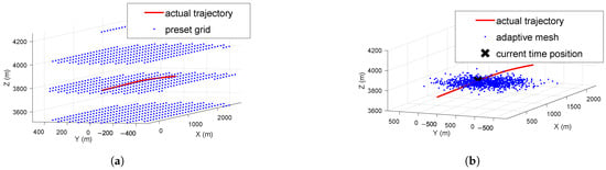
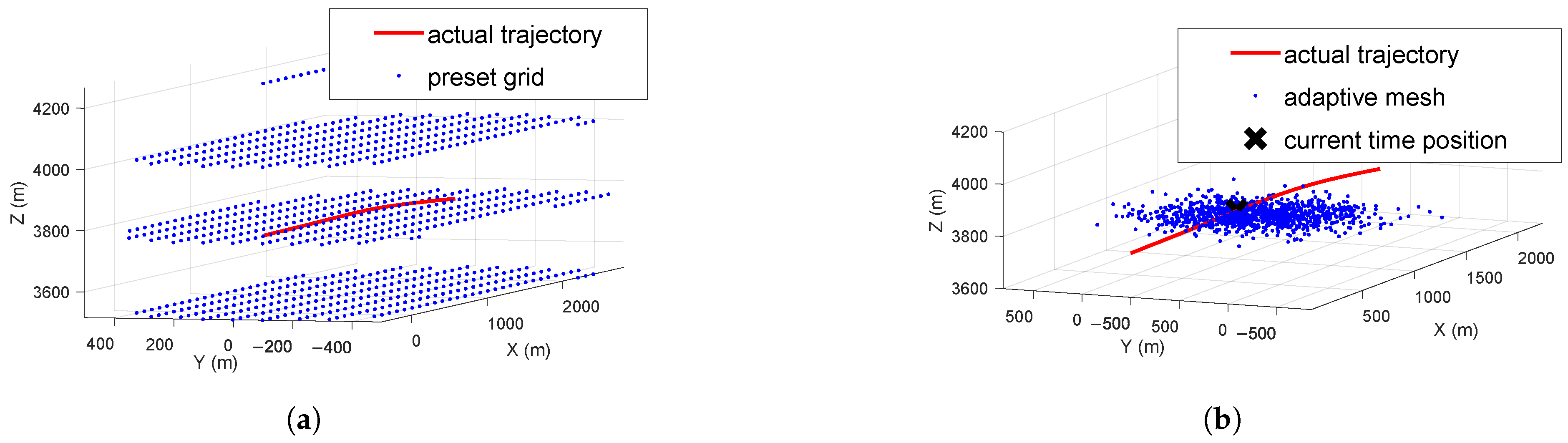
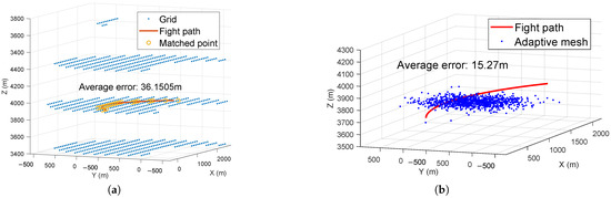
As shown in Figure 4, the fixed grid method is essentially uniform sampling of the state space [23], which cannot reflect the dynamic changes of the state probability distribution; however, through the Bayesian recursive framework, particle filtering ensures that the distribution of the reference grid is always consistent with the carrier motion trend and terrain matching characteristics, thereby realizing the adaptability of the reference grid.

Figure 4. Grid comparison: (a) fixed mesh matching. (b) Adaptive mesh matching.

3.4.2. Particle Filtering Implementation

Monte Carlo Approximation

Particle filtering provides a practical implementation of Bayesian filtering for nonlinear, non-Gaussian systems through Monte Carlo approximation [41]. Rather than computing the posterior probability distribution analytically, which is intractable for our problem, PF approximates the distribution using a set of N weighted particles:

$$\rho \left({\mathbf{x}}_k|{\mathbf{z}}_{1:k}\right)\approx {\displaystyle \sum _{i=1}^N}{w}_k^i\delta \left({\mathbf{x}}_k-{\mathbf{x}}_k^i\right),$$

(14)

where ${\left\{{\mathbf{x}}_k^i,w_k^i\right\}}_{i=1}^N$ represents the particle set, with ${\mathbf{x}}_k^i$ denoting the i-th particle’s state hypothesis and $w_k^i$ denoting its corresponding weight (normalized such that ${\sum }_{i=1}^N{w}_i^k=1$). The Dirac delta function $\delta \left(·\right)$ [42] concentrates probability mass at particle positions.

The key advantage of PF is that it does not require linearization assumptions for the system model or Gaussian noise distributions, and it naturally integrates the complex similarity measurement information from DDM matching, providing a flexible framework for adaptive reference grid generation.

Adaptive Grid Matching Algorithm

The adaptive grid matching algorithm implements a closed-loop “prediction–matching–correction” cycle that integrates PF design with the DDM single-frame matching technology introduced in Section 3.2. Centered on real-time radar echo processing, the algorithm achieves high-precision autonomous positioning in complex scenarios through dynamic reference grid generation, combined-feature similarity calculation, and Bayesian state estimation. The algorithm flow is described in Algorithm 2.

Algorithm 2 Adaptive grid-based matching and positioning algorithm.

Input:  ${\mathcal{R}}_{\mathrm{raw}}$: measured radar echoes; ${\mathit{\mu }}_0,{\mathbf{\Sigma }}_0$: initial state and covariance; ${\mathcal{D}}_{\mathrm{DEM}}$: DEM; ${\mathcal{M}}_{\mathrm{XGB}}$: XGBoost model; ${\mathit{\theta }}_{\mathrm{rad}},{\mathit{\theta }}_{\mathrm{PF}}$: system parameters.

1: Data preprocessing:

Generate ${\mathcal{D}}_{\mathrm{real}}^k$ from ${\mathcal{R}}_{\mathrm{raw}}$ via Algorithm 1; extract INS initial state.

2: Particle prediction:

3: if $k=0$ then

4:     Sample ${\{{\mathbf{x}}_0^i,w_0^i\}}_{i=1}^N\sim \mathcal{N}({\mathit{\mu }}_0,{\mathbf{\Sigma }}_0)$ with $w_0^i=1/N$.

5: else

6:     Propagate ${\mathbf{x}}_{k-1}^i$ to ${\mathbf{x}}_k^i$ via CV/CA model.

7: end if

8: Reference DDM generation:

For each particle ${\mathbf{x}}_k^i$, generate reference DDM ${\mathcal{D}}_{\mathrm{ref}}^{k,i}$ via Algorithm 1.

9: Similarity calculation: Compute similarity $s_k^i={\mathcal{M}}_{\mathrm{XGB}}({\mathcal{D}}_{\mathrm{real}}^k,{\mathcal{D}}_{\mathrm{ref}}^{k,i})$.

10: Weight update: ${\tilde{w}}_k^i\leftarrow s_k^i$ via implicit likelihood model; $w_k^i\leftarrow {\tilde{w}}_k^i/{\sum }_j{\tilde{w}}_k^j$.

11: State estimation: ${\widehat{\mathbf{x}}}_k\leftarrow {\sum }_{i=1}^N{w}_k^i{\mathbf{x}}_k^i$; feed back to next frame.

12: Resampling: Compute the effective sample size $N_{eff}=1/{\sum }_{i=1}^N{\left(w_k^i\right)}^2$. If $N_{eff}<N/2$, resample particles ${\{{\mathbf{x}}_k^i,w_k^i\}}_{i=1}^N$ to obtain ${\{{\widehat{\mathbf{x}}}_k^i,1/N\}}_{i=1}^N$.

Output:  ${\widehat{\mathbf{x}}}_k$: position estimate; ${\{{\widehat{\mathbf{x}}}_k^i,1/N\}}_{i=1}^N$: particle set for next frame.

Discussion

A critical implementation challenge in applying Bayesian filtering to DDM matching is constructing an appropriate likelihood function $\rho \left({\mathbf{z}}_k|{\mathbf{x}}_k\right)$ that quantifies the observation quality given a hypothesized state. Conventional approaches require explicit noise models that are difficult to formulate for the complex, terrain-dependent DDM characteristics identified in Section 2.2. We introduce an implicit likelihood modeling approach that directly utilizes the similarity score output by the XGBoost-based multi-feature matcher:

$$\rho \left({\mathbf{z}}_k|{\mathbf{x}}_k\right)\propto s\left({\mathbf{x}}_k\right),$$

(15)

$s\left(x_k\right)\in \left[0,1\right]$ is the matching similarity produced by the XGBoost ensemble model described in Section 3.2. We note that the similarity score $s\left({\mathbf{x}}_k\right)$ serves as a heuristic surrogate for the likelihood function, as the proportionality constant is not explicitly defined. However, since the subsequent weight normalization eliminates this constant, only the relative ranking of similarity scores influences the particle distribution. The resulting posterior should therefore be interpreted as a practical approximation whose effectiveness is validated empirically through the experimental results in Section 4.

This approach is justified on both theoretical and practical grounds. In the field of statistical signal processing, PF provide a flexible framework that allows matching scores from complex observations, such as terrain elevation and map correlation, to be directly utilized in constructing the likelihood function [43]. Based on the core principles of statistical signal processing and the derivation of DDM matching characteristics, this implicit modeling is mainly based on two points: first, the monotonic consistency between similarity and posterior probability. In statistical signal processing, the core physical meaning of the likelihood function is “the degree of support of observation data for the state”; the closer the state is to the true value, the higher the probability of the observation data appearing. In DDM matching, when the particle position is close to the true position, the feature consistency between the reference DDM and measured DDM is high, and the similarity output by XGBoost is high; when the particle position deviates, the similarity decreases rapidly. This conforms to the physical meaning of the likelihood function. Second, the similarity satisfies non-negativity and normalization feasibility. The likelihood function must satisfy two mathematical conditions: “non-negativity” and “normalizability (integrability)”. In Section 3.2, the XGBoost combined features have constrained the similarity $s\left({\mathbf{x}}_k\right)$ to the interval [0, 1] through regression training, satisfying non-negativity. Meanwhile, in the subsequent particle weight update process of particle filtering, the probability normalization of the likelihood function is realized through “weight normalization”. At this time, the relative magnitude of similarity $s\left({\mathbf{x}}_k\right)$ determines the weight distribution of particles, which meets the calculation requirements of the Bayesian posterior distribution. In engineering practice, this method is equivalent to treating similarity as an implicit observation noise model [44] and completing Bayesian inference through the particle filtering framework. Its effectiveness depends on the ability of the similarity function to truly characterize the observation quality. The XGBoost model itself has strong nonlinear fitting ability, and the similarity $s\left({\mathbf{x}}_k\right)$ it outputs already implicitly models the “state-observation” nonlinear relationship of the DDM.

The adaptive reference matching grid generation method based on PF constructs a closed-loop positioning framework of “state prediction → image matching → weight update → dynamic focusing.” Together with the XGBoost-based multi-feature matching and the fast DDM generation method, this methodology systematically addresses key challenges in DDM-based terrain navigation: fixed reference grid constraints, insufficient robustness of single-feature matching, and poor adaptability to maneuvering platforms.

4. Experiments

This section presents comprehensive experimental validation using both simulated and real airborne SAR altimeter data. The fast DDM generation algorithm is evaluated for terrain information fidelity and computational efficiency. The XGBoost-based multi-feature fusion is assessed against single-feature approaches, and the adaptive particle filtering framework is compared with fixed-grid baselines to verify positioning performance.

4.1. Experimental Setup and Scenario

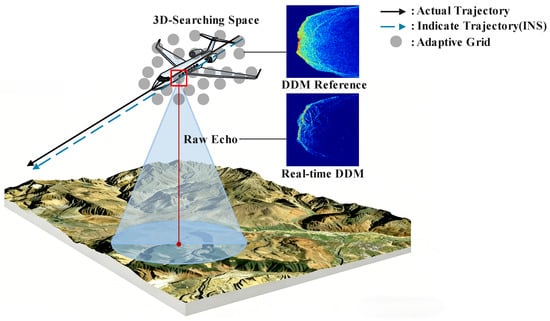
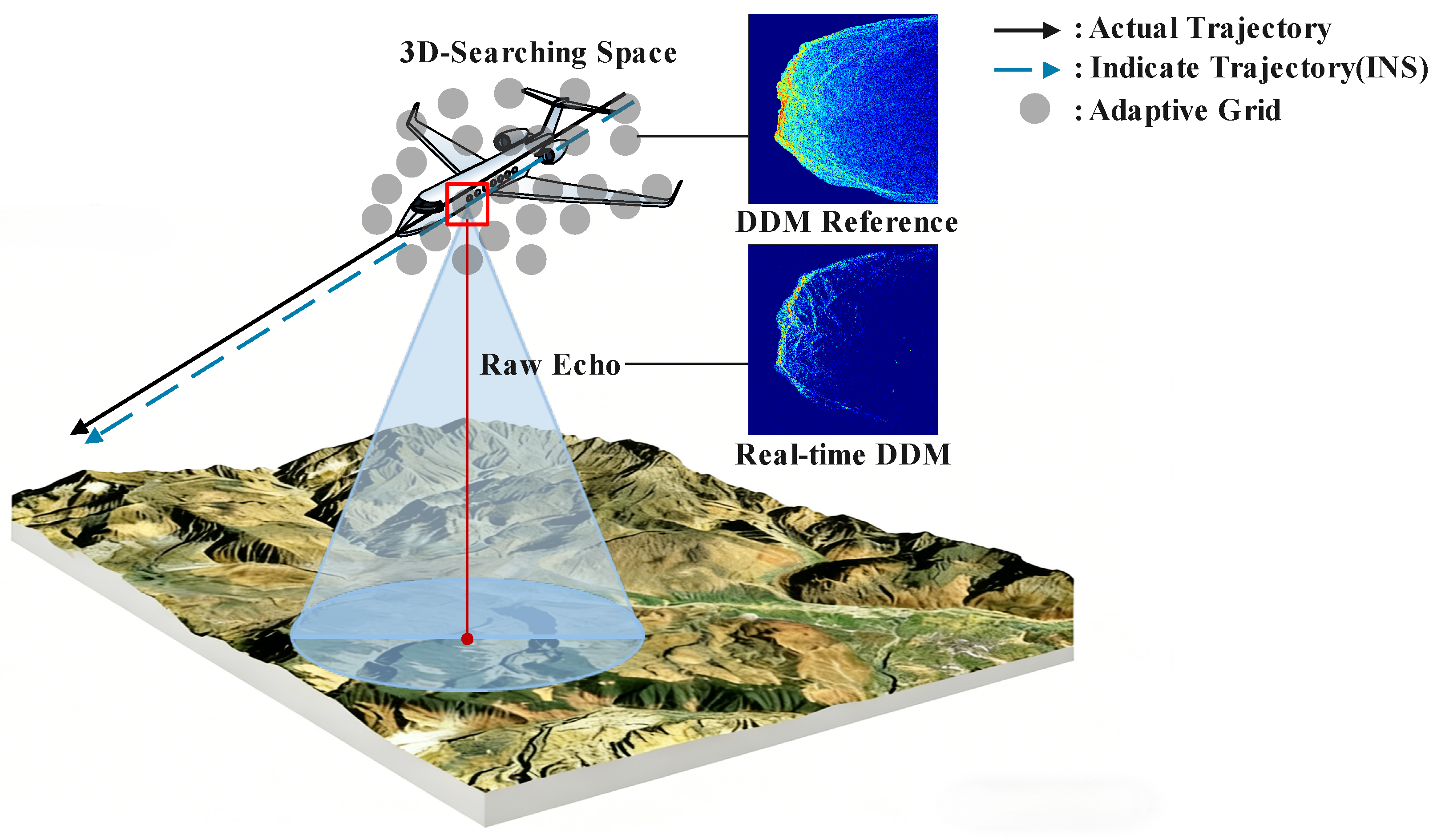
As shown in Figure 5, the experimental data were acquired using a custom nadir-looking X-band airborne SAR altimeter, designated as an NWAPRA (Nadir-looking Wide-beam Autonomous Positioning Radar Altimeter). The complete system specifications are provided in Table 4. The experimental flight area was selected in a mountainous area in Southwest China, which has complex terrain covering various typical terrain types.

Figure 5. The scenario of airborne SAR altimeter.

Table 4. System parameters of the NWAPRA.

Parameter	Value	Parameter	Value
Band	X	Sample Frequency	16.7 MHz
Bandwidth	20 MHz	Pulses of each burst	125
3 dB Beamwidth	60°	Altitude	3.7 km to 3.8 km
PRI	200 μs	Flight Duration	30 s

High-precision Digital Elevation Model (DEM) data with 30 m × 30 m spatial resolution were obtained from the ASTER GDEM V2 global database. The DEM data serve as the ground truth for reference DDM generation and position validation. A tactical-grade INS provides the initial position reference with static accuracy better than 1 m (horizontal) and 2 m (vertical). In the GNSS-denied scenario addressed by this study, the INS-predicted position accumulates drift over time without external corrections, and the maximum search distance $R_{max}=300$ m is designed to encompass this accumulated propagation error. The dynamic velocity measurement accuracy is better than 0.1 m/s with a data sampling interval of 1 s.

4.2. Evaluation Indicators

The test result indicators include positioning error, three-dimensional Root Mean Square Error (3D RMSE), and convergence step size. Positioning error is defined as the three-dimensional Euclidean distance between the actual trajectory points and the matched trajectory points, as shown in Equation:

$$erro{r}_i={∥{\widehat{\mathbf{x}}}_i-{\mathbf{x}}_i∥}_2,$$

(16)

where ${\widehat{\mathbf{x}}}_i$ represents the coordinates of the i-th matched trajectory point and ${\mathbf{x}}_i$ represents the coordinates of the i-th actual trajectory point.

When the algorithm converges, the i-th output position coordinate vector is defined as ${\mathbf{x}}_i^{\mathrm{output}}$, and the i-th true position coordinate vector is defined as ${\mathbf{x}}_i^{\mathrm{true}}$; then, the error vector is defined as ${\mathbf{e}}_i={\mathbf{x}}_i^{\mathrm{output}}-{\mathbf{x}}_i^{\mathrm{true}}$. RMSE represents the root mean square error over the entire trajectory, including the pre-convergence phase, and its calculation formula is expressed as

$$RMSE=\sqrt{{\displaystyle \frac{1}{M}}{\sum }_{i=1}^M{∥{\mathbf{e}}_i∥}_2^2},$$

(17)

where M denotes the total number of trajectory frames. A smaller RMSE indicates higher positioning accuracy.

The convergence step size is defined as the number of frames required from the start of the experiment until the positioning error meets the conditions: the position error of 3 consecutive frames is less than 15 m and the error fluctuation between adjacent frames is less than 5 m. The 15 m threshold corresponds to approximately half the DEM resolution, ensuring that the converged estimate falls within one resolution cell of the true location. The 5 m fluctuation criterion prevents premature convergence when the particle distribution is still evolving. The 3-consecutive-frame requirement provides robustness against transient noise, and the convergence assessment is insensitive to moderate threshold variations. A smaller convergence step size indicates a stronger dynamic response capability of the algorithm.

4.3. Fast DDM Imaging

This section validates that the fast DDM generation algorithm introduced in Section 3.3 maintains sufficient fidelity for terrain matching while achieving substantial computational efficiency gains. The radar echoes were obtained from the measured data of airborne nadir SAR radar. The aircraft was in CV motion at a speed of 75 m/s. One frame of measured echo data was selected and processed with both the traditional finite element method and the fast DDM generation method for comparison.

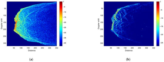
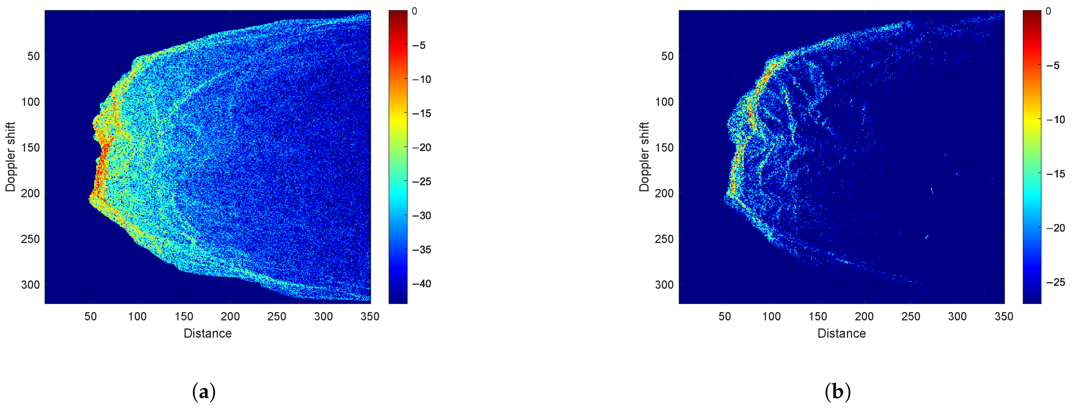
Figure 6 introduces the representative DDM generated by both methods for identical terrain conditions. The energy peak positions and texture distribution trends exhibit excellent correspondence, confirming that the fast method preserves the essential scattering features required for terrain matching. The fast DDM generation algorithm preserves most of the structural and edge texture information, enabling effective image-based matching for positioning while achieving significant computational efficiency gains. SSIM analysis across 10 frames yields 0.6 ± 0.04 (mean ± std). This is validated by the positioning results in subsequent experiments.

Figure 6. Simulated and real DDM: (a) simulated DDM. (b) Real DDM.

Meanwhile, we evaluated the generation time for 10 consecutive DDM frames under identical hardware conditions. The average single-frame generation time of the fast process is 0.91 s compared to 4.52 s for the traditional method, representing a 4.97× speedup. These timings were obtained using a MATLAB (v2023) implementation on a standard laptop and serve as a relative performance benchmark. On embedded platforms based on compiled code (e.g., C++/Verilog), the processing time is expected to be substantially reduced to meet real-time operational requirements.

4.4. XGBoost Feature Importance and Performance Verification

This section validates the effectiveness of the XGBoost ensemble learning framework for DDM similarity assessment.

4.4.1. Dataset Partitioning Strategy

Model training and testing are carried out based on measured trajectory data of 9 segments from an airborne nadir-looking SAR altimeter; the parameter setting of the airborne SAR altimeter is consistent with Table 4. The dataset covers various terrains and flight states. Measured DDMs are generated from measured echoes using the SAR altimeter signal model (Section 2.2), while reference DDMs are generated via fast DDM simulation (Section 3.3) based on INS-predicted positions.

$$Relief=z_L^{\max }-z_L^{\min }.$$

(18)

$$Slope=\arctan \sqrt{{\left({\displaystyle \frac{\partial z_L}{\partial x_L}}\right)}^2+{\left({\displaystyle \frac{\partial z_L}{\partial y_L}}\right)}^2}.$$

(19)

To characterize the terrain diversity, the DEM scatterer areas of all 9 trajectory segments were partitioned into spatial tiles. Each tile was classified by terrain relief and average surface slope, as defined in Equations (18) and (19). As summarized in Table 5, eight distinct terrain types were identified. These span from Hills Flat Terrain to Mid Relief Mild Mountains. The two training trajectories, T2 and T8, were selected to span the full terrain complexity spectrum. T2 covers high-relief steep terrain. T8 covers moderate to low-relief gentle terrain. Together, the training set encompasses 7 of the 8 identified terrain types. The remaining 7 test trajectories contain all 8 types, including Hills Gentle Terrain absent from the training set.

Table 5. Terrain classification of the experimental dataset.

Terrain Type	Relief (m)	Slope ($°$)	Track Coverage
Mid Relief Mild Mountains	500–881	15.1–22.9	T1–T9
Low Relief Gentle Mountains	205–500	7.0–14.9	T1–T9
Mid Relief Gentle Mountains	503–816	8.6–15.0	T1–T9
Hills Undulating Terrain	91–194	2.0–6.5	T6–T9
Low Relief Undulating Mtns	203–338	2.0–6.9	T3, T6–T9
Low Relief Mild Mountains	356–490	15.4–19.2	T1–T7
Hills Flat Terrain	37–134	1.0–1.9	T3, T6–T8
Hills Gentle Terrain	186–192	7.5–8.7	T9

4.4.2. Feature Importance Analysis

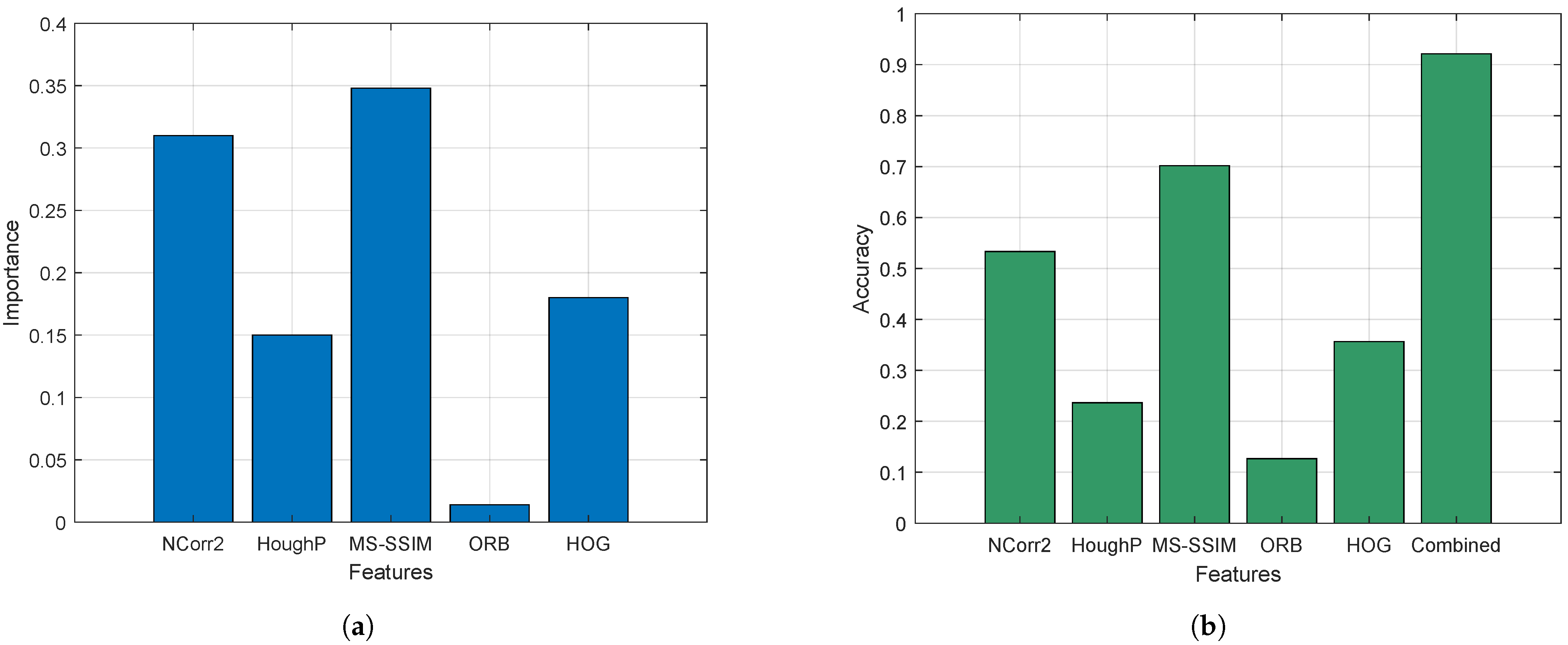
The split gain metric in XGBoost quantifies each feature’s contribution to the decision tree splitting process. Figure 7a introduces the normalized feature importance scores. The dominance of MS-SSIM (34.8%) and NCorr2 (30.1%) confirms that multi-scale structural and grayscale correlation features constitute the core information for DDM matching. The low importance of ORB (1.4%) indicates that point-based features are less effective for nadir-looking DDMs, which typically exhibit sparse distinctive keypoints due to the observation aliasing effect identified in Section 2.2. ORB is retained in the framework as XGBoost automatically downweights low-importance features, and it may still contribute marginally to specific frames where structural features are insufficient. The quantitative feature importance results not only justify our combination strategy but also inform subsequent weight allocation and model optimization. Essentially, it quantifies the contribution of each feature to the spatial position solution of DDM matching.

Figure 7. Performance analysis of XGBoost: (a) the importance proportion of five features. (b) The accuracy of different methods.

4.4.3. Matching Accuracy Comparison

We compare five single features against the combined feature method using matching accuracy (Section 3.2, $\gamma =50$ m). As shown in Figure 7b, MS-SSIM ranks first among single features (70.17%), followed by NCorr2 (53.33%) and HOG (35.67%). Multi-feature fusion improves accuracy to 92.13%, which is a 21.96 percentage point gain over the best single feature. This means that, in the selected reference grid, the combined feature can lock the local area where the real position is located with a higher probability. In this way, the combined feature not only brings higher matching precision but also provides an initial basis for the state focusing of subsequent particle filtering. The combined feature’s high accuracy validates the monotonic similarity–likelihood relationship supporting the implicit likelihood model.

4.5. Adaptive Grid Performance Validation

4.5.1. Comparison Between Fixed Grid and Adaptive Grid

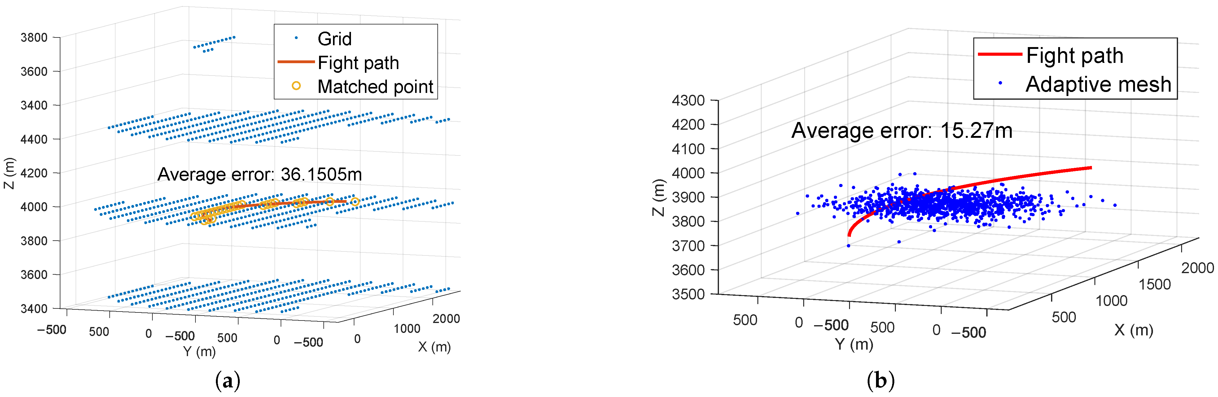
To evaluate the performance advantages of the adaptive grid algorithm, localization experiments were conducted on simulated curved trajectories using both fixed and adaptive grid approaches. As shown in Figure 8, the average positioning error of the fixed grid method is 36.15 m, whereas the adaptive grid method achieves 15.27 m, representing a 57.8% reduction in error. This significant improvement demonstrates that the adaptive grid effectively concentrates computational resources in high-probability regions, eliminating boundary truncation errors inherent to fixed approaches.

Figure 8. Comparison between fixed grid and adaptive grid: (a) Matching positioning of fixed grid. (b) Matching positioning of adaptive grid.

4.5.2. Maneuvering Trajectory Adaptability

To verify the matching and positioning performance under maneuvering conditions, we conducted continuous positioning verification through simulation experiments. The parameters of the simulated SAR altimeter are consistent with those in Table 4. For the trajectory generated by simulated flight, the Constant Velocity (CV) model is used to generate trajectories by adjusting the covariance matrix. We design two simulation scenarios with increasing maneuvering complexity: Scenario A (Gentler Curve): low trajectory curvature with gradual heading changes; Scenario B (More Complex Curve): moderate trajectory curvature with intermittent heading changes. The adaptive grid-based combined feature algorithm is used for matching and positioning in all scenarios.

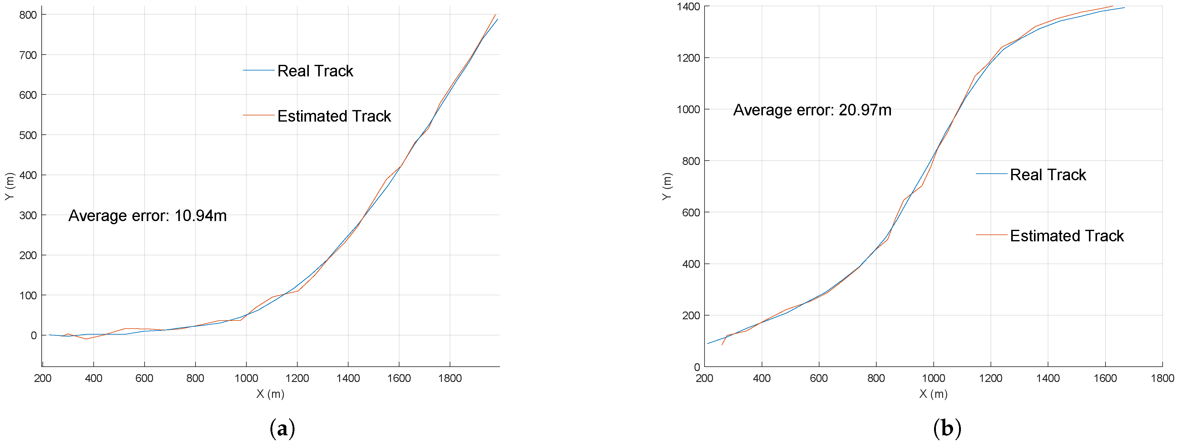
The XY-plane schematics of the matched trajectory and actual trajectory, along with the average positioning errors, are shown in Figure 9a,b. Simulation experiments demonstrate that the adaptive grid matching and positioning algorithm based on combined features exhibits good performance across curved maneuvering trajectories with varying complexity. The dynamic focusing results of adaptive grid particles are further validated through the measured data analysis in Section 4.6, where the evolution of particle probability density under real flight conditions is introduced.

Figure 9. Maneuvering trajectory adaptability: (a) The gentler simulation curve trajectory. (b) A more complex simulation curve trajectory.

4.6. Robustness and Generalization Analysis

4.6.1. Per-Terrain Positioning Performance

To evaluate the per-terrain positioning performance, we grouped the positioning results by the terrain type at each frame’s position according to the classification in Table 5. The aircraft is in a uniform straight flight state. The results are summarized in Table 6. As shown in Table 6, two physically consistent trends are observed: (i) at similar slope levels, higher terrain relief yields lower error, as greater elevation variation produces more distinctive DDM scattering patterns; (ii) at similar relief levels, steeper slopes yield lower error, as steeper surfaces enhance backscatter variation. The positioning results in different terrain types demonstrate the robustness of the proposed framework across diverse terrain conditions.

Table 6. Positioning error performance across terrain types.

Terrain	Mid Relief	Low Relief	Mid Relief	Low Relief	Low Relief	Hills	Hills	Hills
Type	Mild Mtns	Mild Mtns	Gentle Mtns	Gentle Mtns	Und. Mtns	Gentle	Und.	Flat
Error (m)	7.82	13.05	11.20	15.43	25.89	35.27	33.74	41.39

4.6.2. Simulation-Based Validation

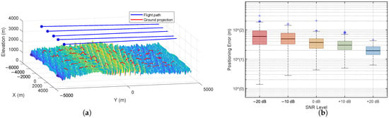
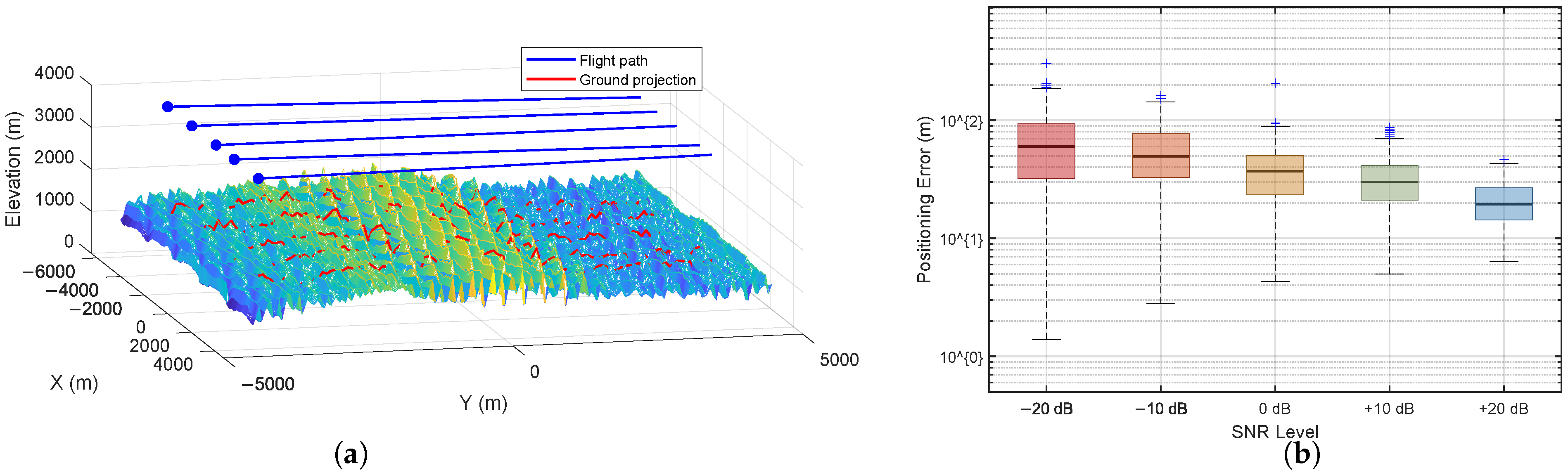
To further verify the generalization of the multi-feature fusion framework, we designed a controlled sim-to-real transfer experiment. A representative complex-terrain region was extracted from the measured DEM. Five virtual flight trajectories were designed over this region, as shown in Figure 10a. Their DDMs were generated using the fast DDM simulation method (Section 3.3). Two of the five simulated trajectories were used to train an XGBoost model. This model was then evaluated on the identical measured-DDM test set used in Section 4.4. As summarized in Table 7, both the measured-DDM and simulated-DDM models achieve high matching accuracy with the same top-two feature ranking. These results confirm that the fusion framework generalizes across independent DDM data sources.

Figure 10. Simulation-based validation: (a) measured terrain with flight trajectories. (b) Distribution of positioning errors under different SNR levels.

Table 7. XGBoost performance with simulated versus measured DDMs for training.

Training DDMs	Train	Test	Acc. (%)	Imp. of NCorr2	Imp. of MS-SSIM
Measured DDMs	T2, T8	T1, T3–T7, T9	92.13	30.1%	34.8%
Simulated DDMs	2 virtual tracks		90.4	47.1%	28.2%

Note: both models are tested on the same measured-DDM test set. “Measured DDMs” are derived from real radar echoes; “Simulated DDMs” are generated over the same measured terrain with virtual flight trajectories.

To evaluate noise robustness, the simulated-DDM model was further tested under varying noise conditions. Multiplicative speckle noise and additive thermal noise were introduced to the DDMs at five SNR levels. Particle filter positioning was evaluated over all five simulated trajectories at each level. As shown in Figure 10b, the RMSE increases monotonically with decreasing SNR. It ranges from approximately 22 m at +20 dB to 81 m at −20 dB. Under moderate-to-high SNR conditions (0 dB to +20 dB), the RMSE remains below 50 m. This confirms that the framework maintains effective positioning accuracy under noise degradation. The elevated baseline RMSE relative to real-data results is attributed to the limited terrain diversity in the simulation environment.

4.7. Measured Data Validation

To validate the method’s effectiveness with real-world data, we utilize original airborne SAR altimeter data over complex terrain. To assess the algorithm’s adaptability to different maneuvers, we conduct three experiments with distinct flight states. In order to verify the superiority of the combined feature method, a contrast experiment with five kinds of single features is designed. In order to show the convergence of the algorithm intuitively, the iterative convergence process diagram and the positioning error convergence are displayed.

4.7.1. Data Acquisition

Three typical trajectory segments were selected for result analysis, with the aircraft’s flight states being uniform linear motion, uniformly accelerated linear motion, and curvilinear motion. The core parameter settings of the SAR altimeter are shown in Table 4. The uniform linear flight trajectory has a speed of 75 m/s with no attitude change; the uniformly accelerated trajectory has an initial speed of 60 m/s and an acceleration of 1 m/s²; the curvilinear trajectory has a speed ranging from 65 m/s to 75 m/s. XGBoost parameters were set consistent with those in Table 2, the division of the training set and test set was the same as in Section 4.2, the maximum search distance was set to 300 m, and the number of initial grid particles was 1000.

4.7.2. Performance Analysis and Discussion

To evaluate the matching and positioning performance of the system algorithm under different scenarios, the RMSE and convergence step size of the system under three scenarios were statistically analyzed, as shown in Table 8. It can be seen that the algorithm exhibits excellent matching and positioning performance under different flight motion scenarios, and all scenarios achieve convergence within 10 steps. In particular, the results of the curvilinear motion scenario show that the algorithm can still achieve effective convergence under complex maneuvers with changes in the carrier’s heading and speed fluctuations, and the RMSE is controlled within 30 m, verifying the good adaptability of the algorithm to maneuvering platforms.

Table 8. Matching and positioning performance in different scenes.

Motion Type	RMSE (m)	Convergence Step Size (Frames)
Uniform Linear Motion	7.82	5
Uniformly Accelerated Linear Motion	11.77	7
Curvilinear Motion	26.33	10

Note: RMSE is computed over the entire trajectory. After convergence, the steady-state error is 6–15 m for the curvilinear motion scenario as shown in Figure 11.

Table 8. Matching and positioning performance in different scenes.

Motion Type	RMSE (m)	Convergence Step Size (Frames)
Uniform Linear Motion	7.82	5
Uniformly Accelerated Linear Motion	11.77	7
Curvilinear Motion	26.33	10

Note: RMSE is computed over the entire trajectory. After convergence, the steady-state error is 6–15 m for the curvilinear motion scenario as shown in Figure 11.

Figure 11. Error of different characteristics in curve trajectory.

Figure 11. Error of different characteristics in curve trajectory.

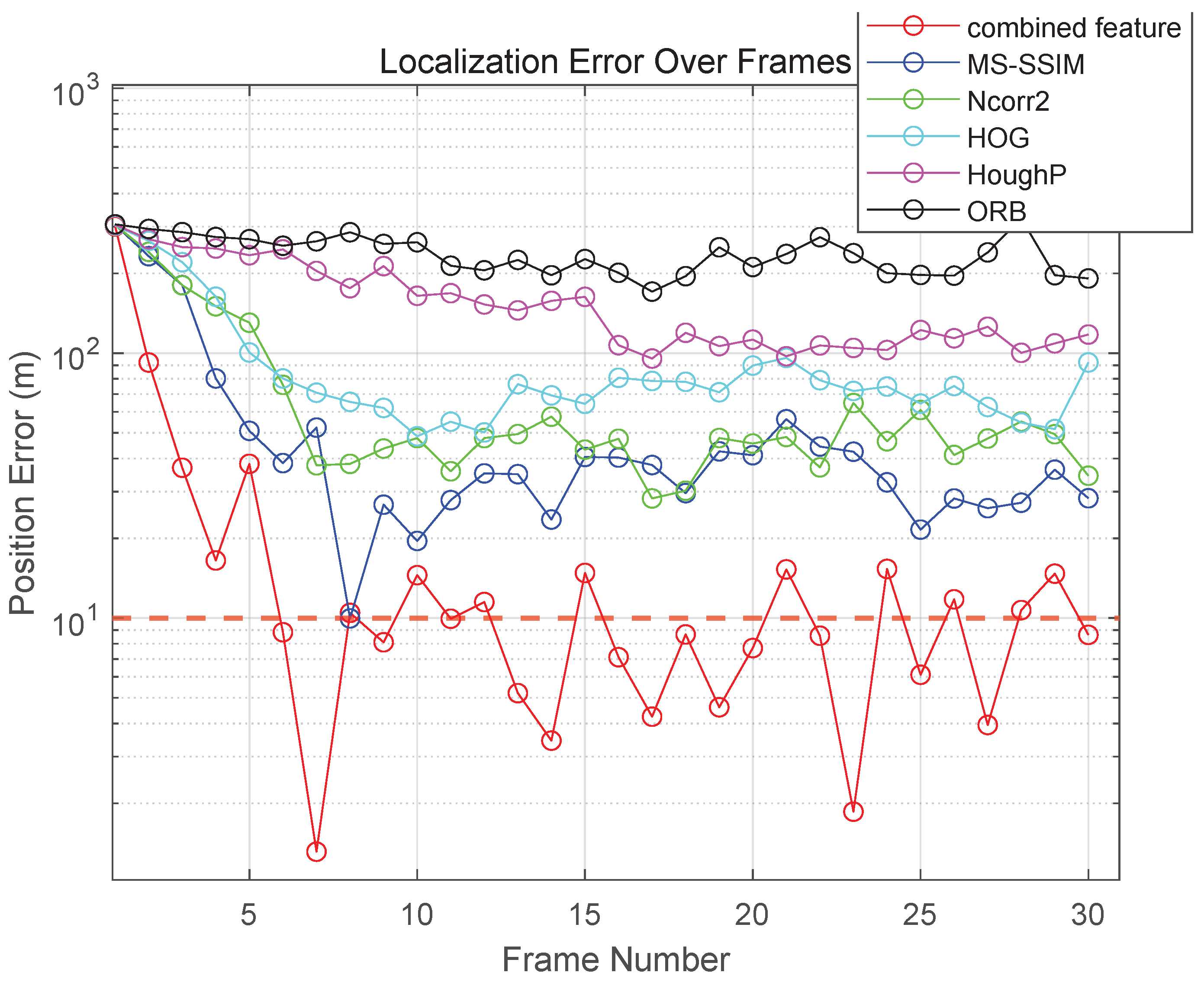
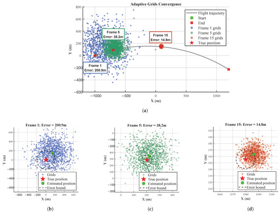
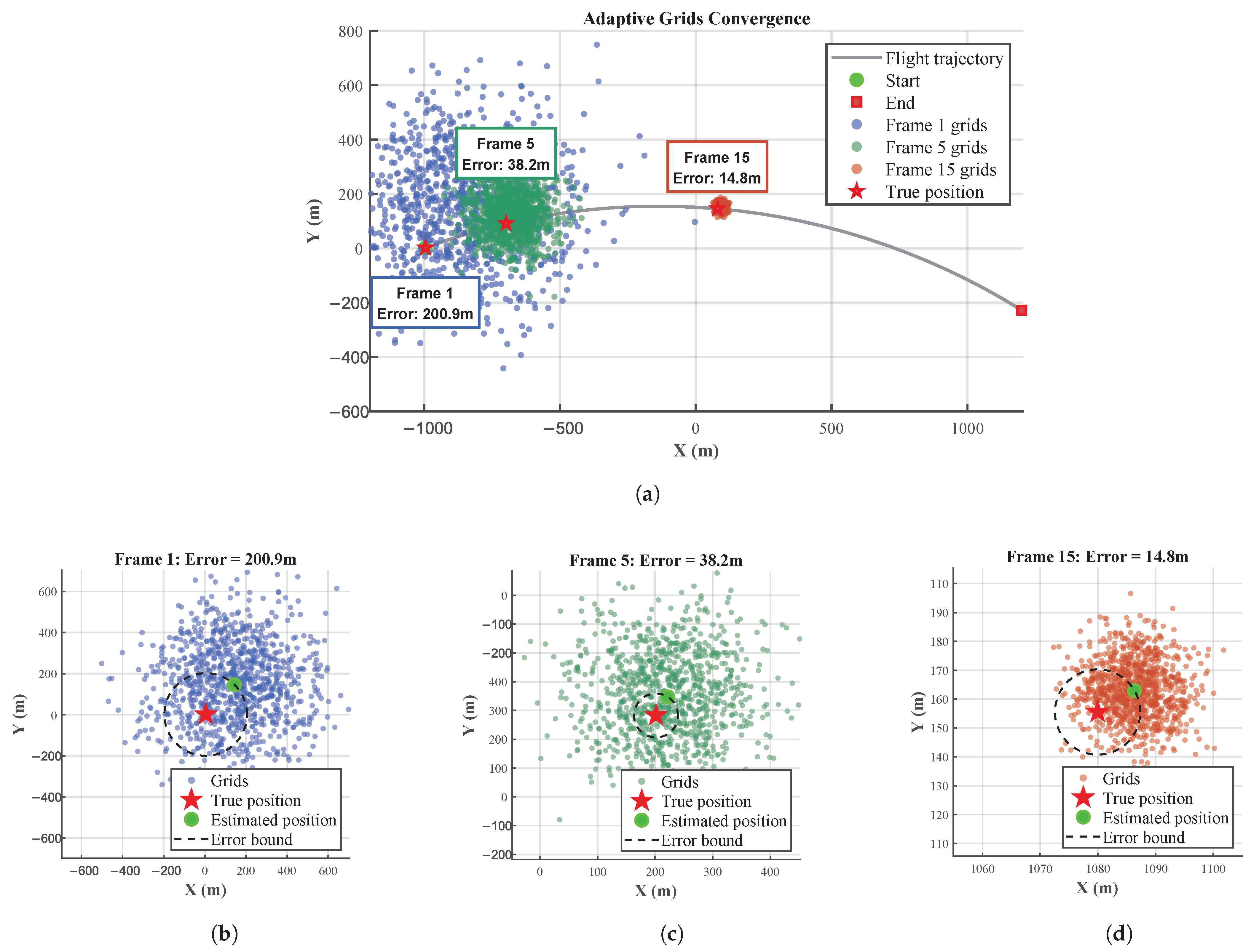
Figure 12 intuitively shows the evolution of the probability density of the grid particles. It can be observed that when the aircraft is in curvilinear flight, the adaptive grid particles can focus on the motion trajectory and flexibly cover the effective echo area. Compared with the fixed grid, the adaptive grid does not require preset trajectory boundaries, can flexibly adapt to changes in the carrier’s heading, avoids the “boundary truncation error” and “redundant sampling in invalid areas” of the fixed grid under maneuvering scenarios, and can meet the matching and positioning requirements of maneuvering flight platforms.

Figure 12. The evolution of the probability density of the grid particles: (a) the convergence process of grid particles. (b–d) The particles and error of Frame 1, Frame 5 and Frame 15.

Figure 11 shows the positioning error convergence results for the most complex curvilinear maneuvering trajectory. As can be seen from the result diagram, compared with the single-feature measurement method, the adaptive matching and positioning system based on the combined-feature measurement method has a faster convergence speed and smaller convergence error: the error can converge to approximately 10 m within about 10 steps, and the minimum error can be reduced to between 3 m and 5 m. Moreover, the combined-feature method maintains fast convergence even with large initial errors, leading to a significant performance improvement. The combined-feature method has stronger robustness: when the initial position error of the carrier is large, the combined feature can still quickly correct the error, while single features such as ORB exhibit error fluctuations and even local divergence.

4.8. Comparative Discussion with Related Works

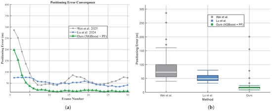
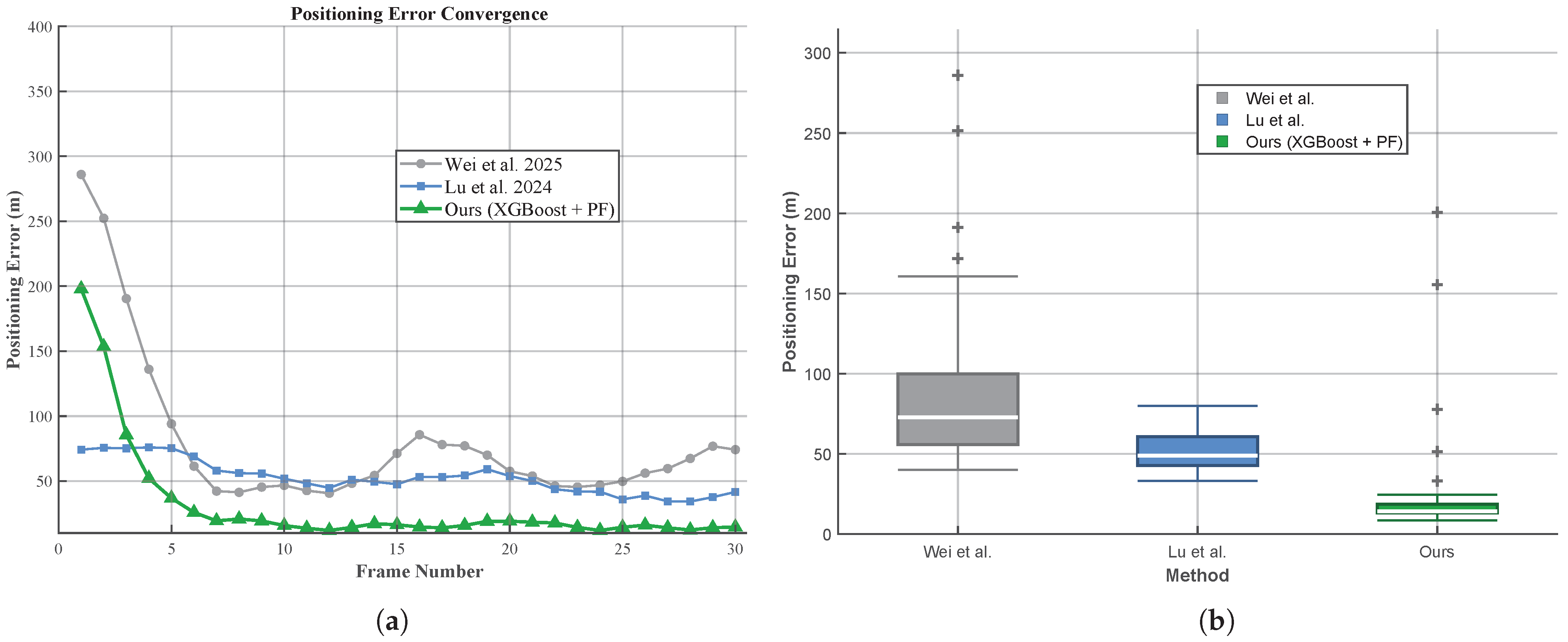
To evaluate the positioning performance under complex maneuvering conditions, comparative experiments were conducted using identical DDM data from the curvilinear motion trajectory. All methods shared the following conditions: maximum search distance of 300 m, particle count of 1000 for grid-based methods, and DEM resolution of 30 m × 30 m. Wei et al.’s method was re-implemented based on the algorithm descriptions in [22] with the parameters reported therein. Lu et al.’s method was evaluated using the original code provided by the authors of [23]. Both baselines were run with their published parameter settings. Figure 13a illustrates the positioning error convergence over 30 frames, revealing distinct behavioral characteristics among methods. Wei et al.’s method exhibits large initial error followed by rapid initial decay, yet subsequently demonstrates sustained fluctuation around 70 m without effective convergence, attributable to the absence of adaptation mechanisms for maneuvering trajectories. Lu et al.’s approach, leveraging deep learning for feature extraction, achieves partial convergence from 70 m to approximately 40 m but continues to exhibit fluctuation due to limited generalization to unseen maneuvering patterns. In contrast, the proposed XGBoost-based adaptive particle filtering framework achieves rapid convergence within approximately 10 frames and finally stabilizes at around 15 m error, demonstrating robust adaptation to complex flight maneuvers. Figure 13b presents the positioning RMSE comparison. The proposed framework achieves 26.33 m RMSE, representing reductions of 70.2% and 48.7% compared to Wei et al. (88.24 m) and Lu et al. (51.35 m), respectively.

Figure 13. Comparison with related works [22,23]: (a) positioning error convergence. (b) Distribution of measured positioning errors.

Each method addresses distinct aspects of the SAR altimeter localization challenge. Wei et al. focus on resolving cross-track ambiguity through spatio-temporal echo similarity analysis, which complements DDM matching. Lu et al. employ end-to-end deep learning for feature extraction, capable of capturing complex nonlinear relationships. Our framework leverages ensemble learning to achieve efficient and stable combined feature matching, while Bayesian sequential estimation enables iterative error convergence through recursive state updates.

5. Conclusions

This paper presents an autonomous wide-beam-tolerant positioning framework integrating Bayesian filtering with Delay-Doppler Map (DDM) matching for terrain-aided navigation in GNSS-denied environments. We established geometric observation and signal models for airborne Synthetic Aperture Radar Altimeters (SAR altimeters) and developed a fast DDM generation algorithm achieving 4.97× computational speedup while maintaining terrain feature fidelity. An XGBoost-based multi-feature similarity learning framework was proposed to adaptively fuse complementary features for robust single-frame matching. Additionally, an adaptive particle filtering framework was developed to construct dynamic reference matching grids, addressing fixed grid constraints, single-feature instability, and limited adaptability to platform maneuvers.

Experimental validation using both simulated and real airborne SAR altimeter data confirmed the effectiveness of the proposed method. The XGBoost-based multi-feature fusion achieved 92.13% matching accuracy, a 21.96 percentage point improvement over the best single feature. Measured data experiments across three motion scenarios yielded RMSE values of 7.82 m (uniform linear), 11.77 m (uniformly accelerated), and 26.33 m (curvilinear), with all scenarios achieving convergence within 10 frames. Comparative experiments on identical datasets demonstrated that the proposed framework achieves 26.33 m RMSE for curvilinear motion, representing reductions of 70.2% and 48.7% compared to Wei et al. (88.24 m) and Lu et al. (51.35 m), respectively.

Limitations of the current work include dependence on pre-trained models, computational demands for resource-constrained platforms, and performance degradation on steep terrain. Future research directions include online learning mechanisms, algorithmic refinements (adaptive particle numbers), hardware acceleration strategies, and multi-modal sensor integration.

References

- Enjolras, V.; Vincent, P.; Souyris, J.-C.; Rodriguez, E.; Phalippou, L.; Cazenave, A. Performances Study of Interferometric Radar Altimeters: From the Instrument to the Global Mission Definition. Sensors 2006, 6, 164–192. [Google Scholar] [CrossRef] [Scilit]
- Lu, J.; Ye, L.; Han, S. Analysis and Application of Geometric Dilution of Precision Based on Altitude Assisted INS/SAR Integrated Navigation. IEEE Trans. Instrum. Meas. 2020, 70, 9501010. [Google Scholar] [CrossRef] [Scilit]
- Ernest, O.; Thomas, P.; B, M.; D, M.; John, B.; Alan, E. GPS-Aided Navigation System Requirements for Smart Munitions and Guided Missiles; American Institute of Aeronautics and Astronautics: New Orleans, LA, USA, 1997. [Google Scholar] [CrossRef] [Scilit]
- Nordlund, P.-J.; Gustafsson, F. Marginalized Particle Filter for Accurate and Reliable Terrain-Aided Navigation. IEEE Trans. Aerosp. Electron. Syst. 2009, 45, 1385–1399. [Google Scholar] [CrossRef] [Scilit]
- Altiparmaki, O.; Amraoui, S.; Kleinherenbrink, M.; Moreau, T.; Maraldi, C.; Visser, P.N.; Naeije, M. Introducing the Azimuth Cutoff as an Independent Measure for Characterizing Sea-State Dynamics in SAR Altimetry. Remote Sens. 2024, 16, 1292. [Google Scholar] [CrossRef] [Scilit]
- Jensen, J.; Raney, R. Delay/Doppler radar altimeter: Better measurement precision. In Proceedings of the IGARSS ’98. Sensing and Managing the Environment. 1998 IEEE International Geoscience and Remote Sensing, Seattle, WA, USA, 6–10 July 1998; Volume 4, pp. 2011–2013. [Google Scholar] [CrossRef] [Scilit]
- Erdem, B.H.; Berkant, A.; Omer, K. Radar altimeter as a navigation aid using hierarchical elevation map clustering. In Proceedings of the 2012 IEEE/ION Position, Location and Navigation Symposium, Myrtle Beach, SC, USA, 23–26 April 2012; IEEE: Piscataway, NJ, USA, 2012; pp. 377–381. [Google Scholar] [CrossRef] [Scilit]
- Li, L.; Yu, Q.; Shang, Y.; Yuan, Y.; Lu, H.; Liu, X. A new navigation approach of terrain contour matching based on 3-D terrain reconstruction from onboard image sequence. China Technol. 2010, 53, 1176–1183. [Google Scholar] [CrossRef] [Scilit]
- Yuan, G.; Zhang, H.; Yuan, K.; Zhu, L. Improved SITAN algorithm in the application of aided inertial navigation. In Proceedings of the 2012 International Conference on Measurement, Information and Control, Harbin, China, 18–20 May 2012; IEEE: Piscataway, NJ, USA, 2012; pp. 922–926. [Google Scholar] [CrossRef] [Scilit]
- Henderson, N.; de Sá Rêgo, M.; Imbiriba, J. Topographical global initialization for finding all solutions of nonlinear systems with constraints. Appl. Numer. Math. 2017, 112, 155–166. [Google Scholar] [CrossRef] [Scilit]
- Bergman, N.; Ljung, L. Terrain navigation using Bayesian statistics. IEEE Control Syst. 1999, 19, 33–40. [Google Scholar] [CrossRef] [Scilit]
- Zhao, L.; Gao, N.; Huang, B.; Wang, Q.; Zhou, J. A novel terrain- aided navigation algorithm combined with the TERCOM algorithm and particle filter. IEEE Sens. J. 2014, 15, 1124–1131. [Google Scholar] [CrossRef] [Scilit]
- Campbell, J.L.; De Haag, M.U. Assessment of radar altimeter performance when used for integrity monitoring in a synthetic vision system. In 20th Digital Avionics Systems Conference; IEEE: Piscataway, NJ, USA, 2001; Volume 1, pp. 2C3/1–2C3/9. [Google Scholar] [CrossRef] [Scilit]
- Ren, S. Research on Key Technologies of Missile-Borne SAR Scene Matching Guidance. Ph.D. Dissertation, National University of Defense Technology, Hunan, China, 2011. [Google Scholar]
- Xin, R.; Zhang, X.; Peng, X.; Chen, J. UFormer: End-to-End feature point scene matching algorithm based on Transformer and U-Net structure. J. Comput. Sci. 2023, 50, 334–339. [Google Scholar]
- Li, B.; Wu, J.; Zhang, D.; Zhu, H.; Hu, C.; Bai, S. Adaptive screening method of scene matching area based on convolutional neural network. J. Rocket. Force Eng. Univ. 2024, 38, 45–50. [Google Scholar]
- Liaghat, A.; Helfroush, M.S.; Norouzi, J.; Danyali, H. Airborne SAR to optical image registration based on SAR geo-referencing and deep learning approach. IEEE Sens. J. 2023, 23, 26446–26458. [Google Scholar] [CrossRef] [Scilit]
- Semenov, A.; Rysz, M.; Demeyer, G. Deep Learning Approach for SAR Image Retrieval for Reliable Positioning in GPS-Challenged Environments. IEEE Trans. Geosci. Remote Sens. 2024, 62, 5106011. [Google Scholar] [CrossRef] [Scilit]
- Zhang, Z.; Zhang, X. A Review of Research on Generalization Error Analysis of Deep Learning Models. In International Conference on Image Processing, Computer Vision and Machine Learning; IEEE: Piscataway, NJ, USA, 2023; pp. 906–912. [Google Scholar] [CrossRef] [Scilit]
- Raney, R.K. The Delay/Doppler Radar Altimeter. IEEE Trans. Geosci. Remote Sens. 1998, 36, 1578–1588. [Google Scholar] [CrossRef] [Scilit]
- Chen, C.; Li, X.; Zhu, J.; Peng, H.; Xue, Y.; Zhai, W.; Lin, M.; Zhang, Y.; Liu, J.; Zhao, Y. Research on the Algorithm of Lake Surface Height Inversion in Qinghai Lake Based on Sentinel-3A Altimeter. Remote Sens. 2025, 17, 647. [Google Scholar] [CrossRef] [Scilit]
- Wei, Y.; Qin, W.; Hu, F. SAR altimeter 3-D localization with combined Delay Doppler Image and spatio-temporal echo similarity. Isprs J. Photogramm. Remote Sens. 2025, 223, 46–57. [Google Scholar] [CrossRef] [Scilit]
- Lu, Y.X.; Song, A.; Liu, G.Z.; Tan, L.L.; Xu, Y.S.; Li, F.; Wang, Y.; Jiang, G.; Yang, L. TMP-Net: Terrain Matching and Positioning Network by Highly Reliable Airborne Synthetic Aperture Radar Altimeter. Remote Sens. 2024, 16, 2966. [Google Scholar] [CrossRef] [Scilit]
- Hou, H.; Qu, C.; Zhou, Q.; Xiang, Y. A Downward-looking Three-dimensional Imaging Method for Airborne FMCW SAR Based on Array Antennas. Chin. J. Aeronaut. 2011, 24, 55–64. [Google Scholar] [CrossRef] [Scilit]
- Yang, S.; Zhang, Z.; Xu, K.; Wang, Z.; Shi, L.; Wang, L.; Chen, H. The ground process segment of SAR altimeter. Remote Sens. Technol. Appl. 2017, 32, 1083–1092. [Google Scholar]
- Zhu, Z.; Zhang, H. Raw signal simulation of synthetic aperture radar altimeter over complex terrain surfaces. Radio Sci. 2020, 55, e2019RS006948. [Google Scholar] [CrossRef] [Scilit]
- Xu, G.; Chen, Y.; Ji, A.; Zhang, B.; Yu, C.; Hong, W. 3-D High-Resolution Imaging and Array Calibration of Ground-Based Millimeter-Wave MIMO Radar. IEEE Trans. Microw. Theory Tech. 2024, 72, 4919–4931. [Google Scholar] [CrossRef] [Scilit]
- Misra, I.; Rohil, M.K.; Moorthi, S.M.; Dhar, D. Feature based remote sensing image registration techniques: A comprehensive and comparative review. Int. J. Remote Sens. 2022, 43, 4477–4516. [Google Scholar] [CrossRef] [Scilit]
- Nadir, M.B.; Youcef, B.; Miloud, C.E. FPGA implementation of feature detection and matching using ORB. Microprocess. Microsyst. 2022, 94, 104666. [Google Scholar] [CrossRef] [Scilit]
- Gintautas, P. Image similarity/distance measures: What is really behind MSE and SSIM? Int. J. Image Data Fusion 2017, 8, 32–53. [Google Scholar] [CrossRef] [Scilit]
- Wu, Z.; Mao, K.; Ng, G.-W. Enhanced feature fusion through irrelevant redundancy elimination in intra-class and extra-class discriminative correlation analysis. Neurocomputing 2019, 335, 105–118. [Google Scholar] [CrossRef] [Scilit]
- Chen, T.; Guestrin, C. XGBoost: A Scalable Tree Boosting System. In KDD ’16: Proceedings of the 22nd ACM SIGKDD International Conference on Knowledge Discovery and Data Mining; Association for Computing Machinery: New York, NY, USA, 2016; pp. 785–794. [Google Scholar] [CrossRef] [Scilit]
- Deng, Y.; Lumley, T. Multiple Imputation Through XGBoost. J. Comput. Graph. Stat. 2024, 33, 352–363. [Google Scholar] [CrossRef] [Scilit]
- Blaber, J.; Adair, B.; Antoniou, A. Ncorr: Open-Source 2D Digital Image Correlation Matlab Software. Exp. Mech. 2015, 55, 1105–1122. [Google Scholar] [CrossRef] [Scilit]
- Devi, M.G.; Akila, I.S. Image fusion: A deep Y shaped-residual convolution auto-encoder with MS-SSIM loss function. J. Radiat. Res. Appl. Sci. 2024, 17, 101089. [Google Scholar] [CrossRef] [Scilit]
- Cheng, L.; Fang, J.; Wu, Y.; Kang, K. Research on improved image edge detection based on Hough transform. Int. Conf. Image Process. Intell. Control 2021, 11928, 146–150. [Google Scholar] [CrossRef] [Scilit]
- Zhang, X.; Shangguan, H.; Ning, A.; Wang, A.; Zhang, J.; Peng, S. Pedestrian Detection with EDGE Features of Color Image and HOG on Depth Images. Control Comp. Sci. 2020, 54, 168–178. [Google Scholar] [CrossRef] [Scilit]
- Bentoumi, M.; Daoud, M.; Benaouali, M.; Taleb Ahmed, A. Improvement of emotion recognition from facial images using deep learning and early stopping cross validation. Multimed. Tools Appl. 2022, 81, 29887–29917. [Google Scholar] [CrossRef] [Scilit]
- Kulemin, G.P. Millimeter-Wave Radar Targets and Clutter; Artech House: Norwood, MA, USA, 2003. [Google Scholar]
- Li, X.R. Survey of maneuvering target tracking. Part I. Dynamic models. IEEE Trans. Aerosp. Electron. Syst. 2003, 39, 1333–1364. [Google Scholar] [CrossRef] [Scilit]
- Gustafsson, F.; Gunnarsson, F.; Bergman, N.; Forssell, U.; Jansson, J.; Karlsson, R. Particle filters for positioning, navigation, and tracking. IEEE Trans. Signal Process. 2002, 50, 425–437. [Google Scholar] [CrossRef] [Scilit]
- Xiubin, X. Nonlinear trigonometric approximation and the Dirac delta function. J. Comput. Appl. Math. 2007, 209, 234–245. [Google Scholar] [CrossRef] [Scilit]
- Karlsson, R.; Gustafsson, F. Bayesian Surface and Underwater Navigation. IEEE Trans. Signal Process. 2006, 54, 4204–4214. [Google Scholar] [CrossRef] [Scilit]
- Michael, M.; Sebastian, T.; Daphne, K.; Ben, W. FastSLAM: A factored solution to the simultaneous localization and mapping problem. Am. Assoc. Artif. Intell. 2002, 593598, 593–598. [Google Scholar]
Disclaimer/Publisher’s Note: The statements, opinions and data contained in all publications are solely those of the individual author(s) and contributor(s) and not of MDPI and/or the editor(s). MDPI and/or the editor(s) disclaim responsibility for any injury to people or property resulting from any ideas, methods, instructions or products referred to in the content. |
© 2026 by the authors. Licensee MDPI, Basel, Switzerland. This article is an open access article distributed under the terms and conditions of the Creative Commons Attribution (CC BY) license.