Extracting Alpine Shrub Using Improved Lightweight DeepLabV3+ Network

Highlights

What are the main findings?

• An improved lightweight DeepLabV3+ model was adapted for alpine shrub segmentation from high-resolution UAV imagery.
• The integrated use of MobileNetV2, cSE, and GhostConv improved the balance between segmentation accuracy and model complexity.

What are the implications of the main findings?

• The method provides a practical approach for fine-scale alpine shrub mapping under fragmented and heterogeneous background conditions.
• This study supports UAV-based alpine vegetation monitoring and provides a data scenario for lightweight shrub extraction in alpine ecosystems.

Abstract

In recent years, shrubland is an important land cover type in alpine regions, while accurate segmentation of shrubs using remote sensing data remain challenging. To address these issues, this study proposes an alpine shrub segmentation method based on an improved lightweight DeepLabV3+ network, in which MobileNetV2 is used to replace the original backbone to reduce model complexity while maintaining feature representation capability, a channel squeeze-and-excitation (cSE) attention module is introduced to enhance the response to key shrub features and boundary details, and Ghost convolution is incorporated to reduce computational redundancy while preserving segmentation accuracy. Experimental results from both ablation and comparative studies demonstrate that the proposed model achieves a mean intersection over union (MIoU) of 88.47%, mean pixel accuracy (mPA) of 92.93%, F1-score of 91.80%, and overall accuracy of 94.52%, representing improvements of 3.53%, 2.64%, 2.96%, and 1.69%, respectively, over the original DeepLabV3+ model, while also significantly reducing the number of parameters and model size. In addition, independent cross-year validation using unmanned aerial vehicle (UAV) imagery acquired in 2025 suggests that the proposed model has good applicability under similar UAV sensor and acquisition conditions. Overall, this study provides an effective lightweight semantic segmentation approach for alpine shrub segmentation from high-resolution UAV imagery and offers useful technical support for vegetation monitoring in alpine regions such as the Qinghai–Tibet Plateau.

1. Introduction

Alpine shrubs are a characteristic vegetation type found in high-altitude regions, playing a crucial role in ecosystem functioning, including carbon and nitrogen cycling, biodiversity conservation, and the maintenance of ecosystem stability. In recent decades, shrub expansion has been widely observed across tundra and alpine ecosystems, driven by global climate warming and anthropogenic disturbances. This phenomenon, often referred to as shrub encroachment, has attracted increasing attention due to its profound impacts on vegetation structure and ecological processes [1,2,3]. Previous studies have shown that shrub expansion can significantly alter plant community composition, reduce grassland productivity, and modify soil moisture and nutrient distribution patterns, thereby affecting the overall resilience of ecosystems [4]. Therefore, accurately extracting the spatial distribution of alpine shrubs and monitoring their expansion dynamics is essential for understanding vegetation succession and supporting ecological management in alpine regions.

The segmentation of alpine shrubs from remote sensing imagery presents a significant challenge. Unlike cultivated vegetation or structurally homogeneous shrublands, alpine shrubs are typically characterized by their low stature, fragmented distribution patterns, and strong spatial heterogeneity. In high-resolution UAV imagery, these shrubs are often intermingled with grasslands bare soil, gravel surfaces, and shadowed areas, leading to blurred boundaries and high spectral similarity with adjacent land cover types. This “same-spectrum–different-object” phenomenon significantly increases the difficulty of accurate classification and segmentation [5]. In addition, the irregular morphology and discontinuous spatial distribution of alpine shrub patches make it difficult for conventional methods to preserve fine boundary details and identify small shrub targets in heterogeneous alpine environments. Traditional approaches to shrub segmentation primarily encompass manual visual interpretation, pixel-based classification, and classical machine learning techniques. Although manual interpretation can achieve high accuracy, it is time-consuming, labor-intensive, and challenging to apply at large spatial scales. In contrast, pixel-based classification methods offer greater automation; however, they are frequently constrained by lower accuracy in complex environments [6]. Machine learning algorithms such as random forest and support vector machines have been widely applied in remote sensing classification tasks due to their robustness and relatively high performance [7]. However, their effectiveness largely depends on feature engineering and data quality, and their generalization ability is often limited in heterogeneous landscapes [8].

In recent years, deep learning has emerged as a dominant paradigm in the analysis of remote sensing image and semantic segmentation. Notable models such as Fully Convolutional networks (FCNs), U-Net, PSPNet, SegNet and the DeepLab series have demonstrated remarkable capabilities in extracting complex land cover features from high-resolution imagery [9,10,11,12,13]. Compared to traditional methods, deep learning-based approaches can automatically learn hierarchical feature representations and effectively capture spatial context information. Specifically, semantic segmentation models have exhibited significant advantages in delineating object boundaries and identifying fragmented targets, making them particularly suitable for vegetation segmentation tasks in complex environments [14,15]. Recent studies have further advanced remote sensing semantic segmentation by improving multi-scale feature representation, boundary refinement, and generalization under complex scenes. For example, MCCANet introduces boundary supervision-aided multi-scale channel-wise cross attention to enhance feature fusion and boundary preservation in high-resolution remote sensing images [16]. With the development of vision foundation models, SAM-based frameworks have also been explored for remote sensing segmentation. SAM-DBNet incorporates the Segment Anything Model into a dual-branch network to strengthen feature representation for remote sensing semantic segmentation [17]. More recently, HyperR3SNet has attempted to leverage vision foundation models and hyperbolic representation learning to improve segmentation generalization under limited annotations and complex scale variations [18]. These studies indicate that effective segmentation in complex remote sensing scenes depends not only on global semantic representation, but also on multi-scale feature fusion, boundary-aware refinement, and robust generalization ability. Among existing semantic segmentation frameworks, the DeepLab series stands out as a representative multi-scale segmentation framework and has been extensively utilized as a baseline for further enhancements. Within this series, DeepLabV3 enhances semantic segmentation through the implementation of atrous spatial pyramid pooling (ASPP) module to capture multi-scale contextual information. DeepLabV3+ further expands this framework by incorporating an encoder–decoder structure, thereby improving spatial detail recovery and object boundary delineation [19]. Therefore, DeepLabV3+ has been widely adopted in semantic segmentation tasks due to its ability to integrate multi-scale contextual features and recover boundary details. However, despite its robust performance, the original DeepLabV3+ model is hindered by limitations such as a large parameter size, high computational cost, and relatively slow inference speed, which restrict its deployment in resource-constrained environments. Additionally, the absence of an effective mechanism for emphasizing key feature channels may diminish its capacity to capture fine-grained details of alpine shrubs against complex backgrounds.

To address the need for accurate and efficient segmentation of alpine shrubs, this study proposes an improved lightweight DeepLabV3+ model for alpine shrub segmentation. Specifically, MobileNetV2 is utilized as the backbone network to reduce model complexity while preserving the capability for effective feature segmentation [20]. Additionally, a channel squeeze-and-excitation (cSE) attention module is introduced to enhance the model’s ability to focus on shrub-related features while suppressing background noise [21]. 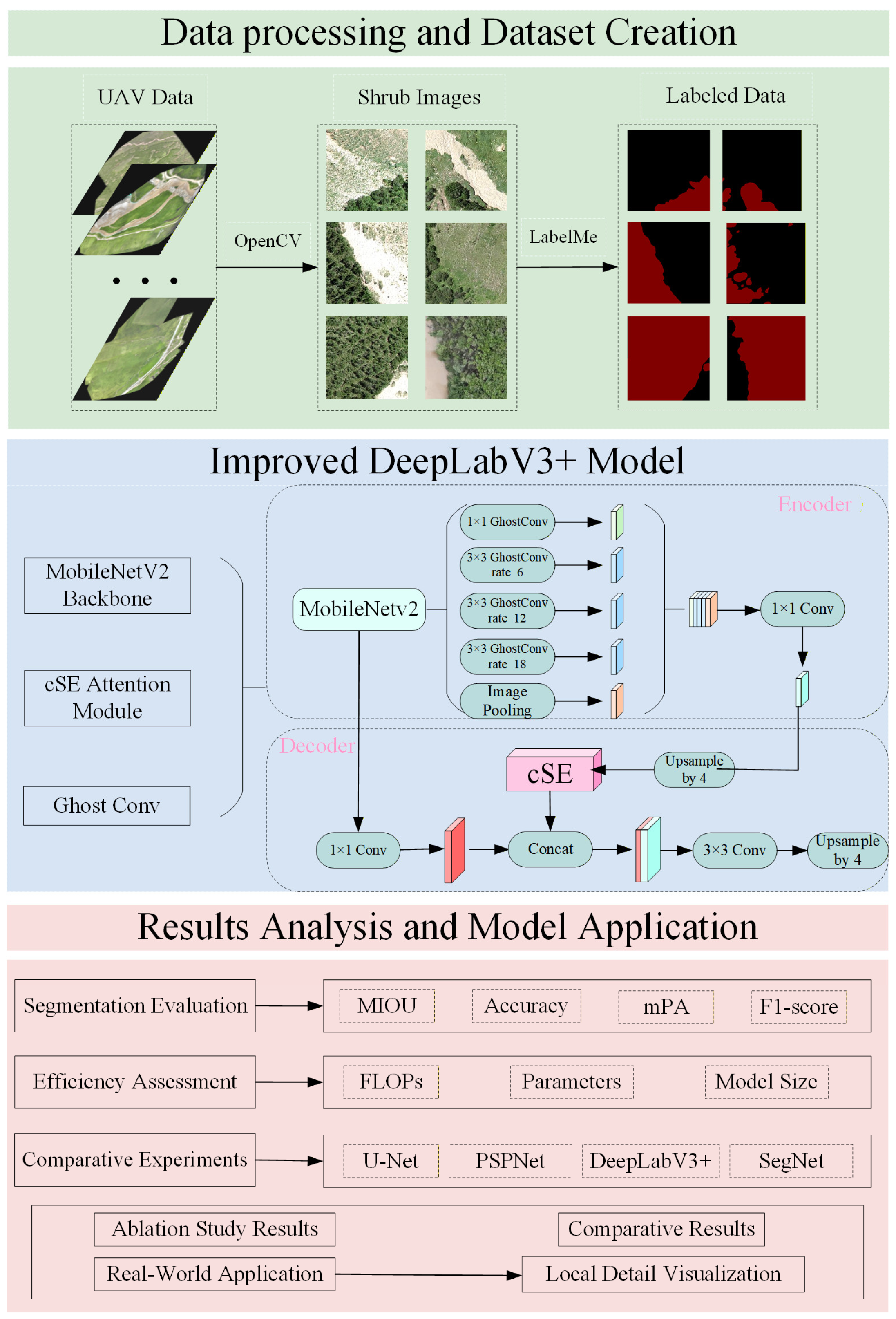Furthermore, Ghost convolution is integrated into the ASPP module to minimize redundant computations and improve computational efficiency without sacrificing segmentation accuracy [22]. Through the integration of lightweight design, attention mechanisms, and efficient convolutional operations, the proposed model aims to achieve a better balance between segmentation accuracy and inference efficiency. The technical workflow of this study is shown in Figure 1, encompassing data processing, dataset creation, the construction of the improved DeepLabV3+ model, and results analysis. This includes segmentation evaluation, efficiency assessment, comparative experiments, ablation studies, and real-world visualization.

2. Materials and Methods

2.1. Data Acquisition and Dataset Construction

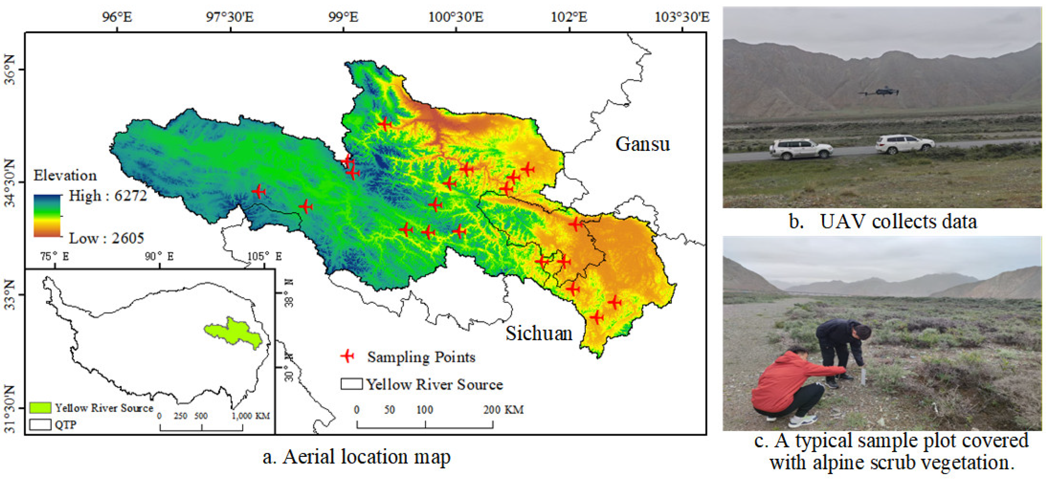
To investigate the distribution of alpine shrubs on the Qinghai–Tibet Plateau, field surveys were conducted in the source region of the Yellow River within Sanjiangyuan National Park in June 2024 and July 2025. Typical shrub distribution areas were surveyed using a DJI unmanned aerial vehicle platform equipped with an RGB camera (Mavic 3 Enterprise, M3E, DJI, Shenzhen, China). The UAV flight parameters were optimized for favorable weather conditions, including sunny weather, wind speed ≤ 4 m/s, a flight altitude of 100 m, 80% forward overlap, 70% side overlap, and a ground sampling distance of 2.74 cm at the image center. The camera had an equivalent focal length of 12 mm and an aperture of F2.8.

Based on the UAV 3D photogrammetry module, automatic flight route planning and image acquisition were executed for 20 study plots. The raw images underwent processing that included image quality inspection, feature point matching, aerial triangulation, point cloud generation, digital surface model construction, orthorectification, and image mosaicking to generate centimeter-level RGB orthomosaic images of the study plots. During this process, geometric correction, terrain-related displacement correction, and orthorectification were performed to minimize geometric distortion in the original UAV images. The spatial distribution of the study plots is shown in Figure 2a, while the field data acquisition process is depicted in Figure 2b,c. UAV images obtained in 2024 were primarily utilized for model training and internal validation, whereas UAV images collected in 2025 were excluded from model training and parameter tuning. Instead, these images served as an independent validation dataset to further assess the model’s applicability under cross-year UAV image conditions.

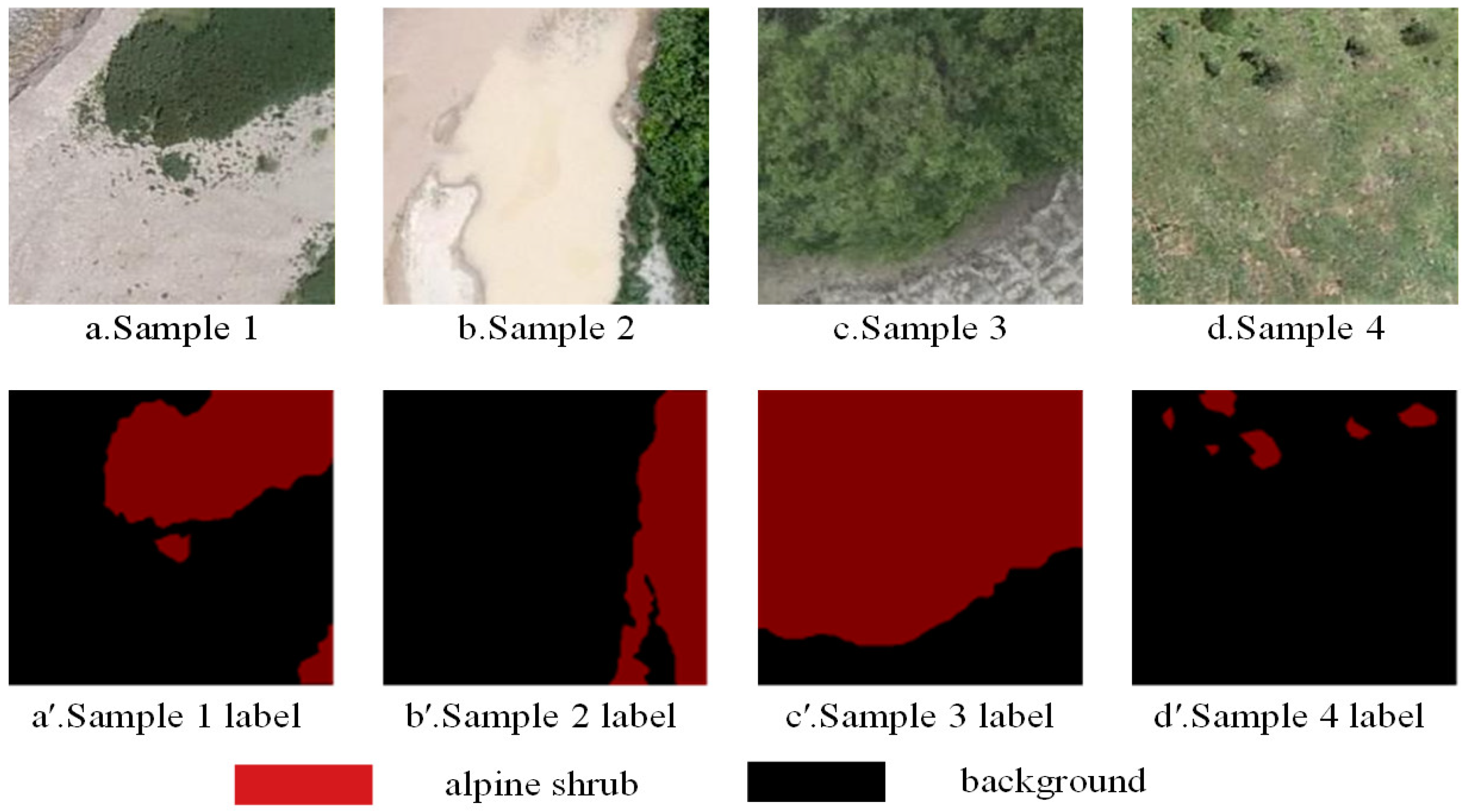
The generated UAV orthomosaic images were subsequently cropped into standardized patches of 256 × 256 pixels. Following the screening and removal of duplicate or low-quality samples, a total of 959 alpine shrub images were acquired. These images were manually annotated using the polygon labeling tool in LabelMe (version 3.16.7), generating corresponding annotation files in JSON format. The annotations were then converted into binary masks for model training and validation, with shrub pixels labeled as 0 and background pixels labeled as 1. Representative examples of the original alpine shrub images and their corresponding annotations are shown in Figure 3.

2.2. Data Augmentation

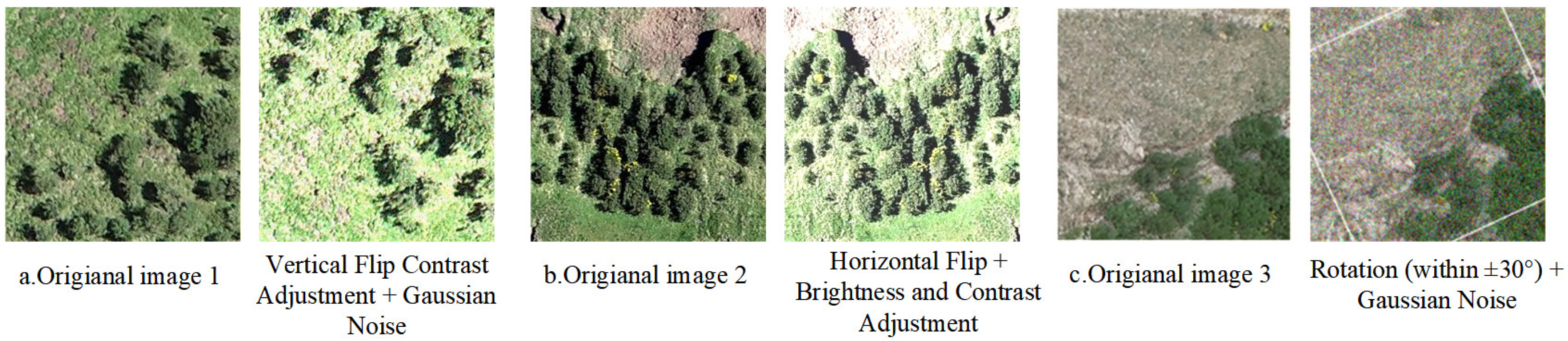
To increase the diversity of the dataset and improve the model’s adaptability to different scene conditions, data augmentation was applied to the original images. The augmentation strategies included both geometric and non-geometric transformations. The geometric transformations consisted of horizontal flipping, vertical flipping, random rotation within ±30°, and random cropping. The non-geometric transformations included random adjustments of brightness and contrast, as well as the addition of Gaussian noise. During the augmentation process, each image was subjected to one geometric transformation and two non-geometric transformations in sequence. After augmentation, the dataset was expanded to 3836 images. To avoid potential data leakage between the training and validation sets, the augmented samples were divided using an original-image-level grouping strategy. Specifically, all augmented versions generated from the same original image were assigned to the same subset, ensuring that no augmented version of the same original image appeared simultaneously in both the training and validation sets. The dataset was then divided into a training set and a validation set at a ratio of 8:2, resulting in 3069 training images and 767 validation images. Examples of the augmented images are shown in Figure 4.

2.3. DeepLabV3+ Network

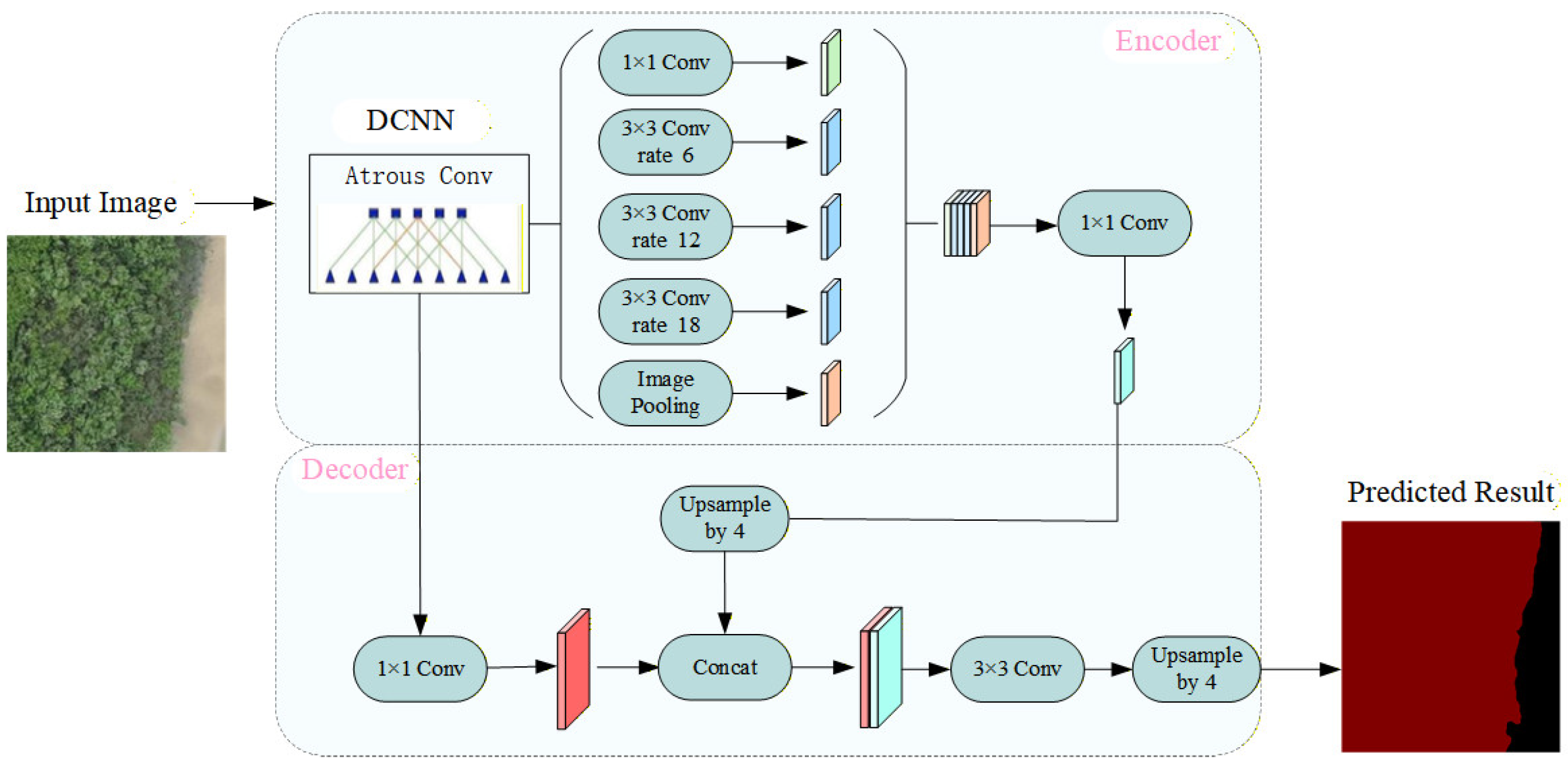
DeepLabV3+ is a widely used semantic segmentation framework proposed by Chen et al. [15] which extends DeepLabV3 by introducing an encoder–decoder architecture to effectively integrate high-level semantic information with low-level spatial details, thereby improving segmentation accuracy. The model incorporates an Atrous Spatial Pyramid Pooling (ASPP) module, which applies parallel atrous convolutions with different dilation rates together with global average pooling to capture multi-scale contextual information and enlarge the receptive field. In the encoder stage, deep convolutional layers are used to extract high-level semantic features from the input image, while in the decoder stage, these features are fused with low-level features from earlier layers to recover spatial resolution and refine object boundaries. Through the combination of multi-scale feature segmentation and feature fusion, DeepLabV3+ enables accurate pixel-level segmentation. However, despite its strong performance, the original model still suffers from relatively high computational cost and large parameter size, which may limit its deployment in resource-constrained scenarios. The network architecture of DeepLabV3+ is shown in Figure 5.

2.4. Improved DeepLabV3+ Semantic Segmentation Model

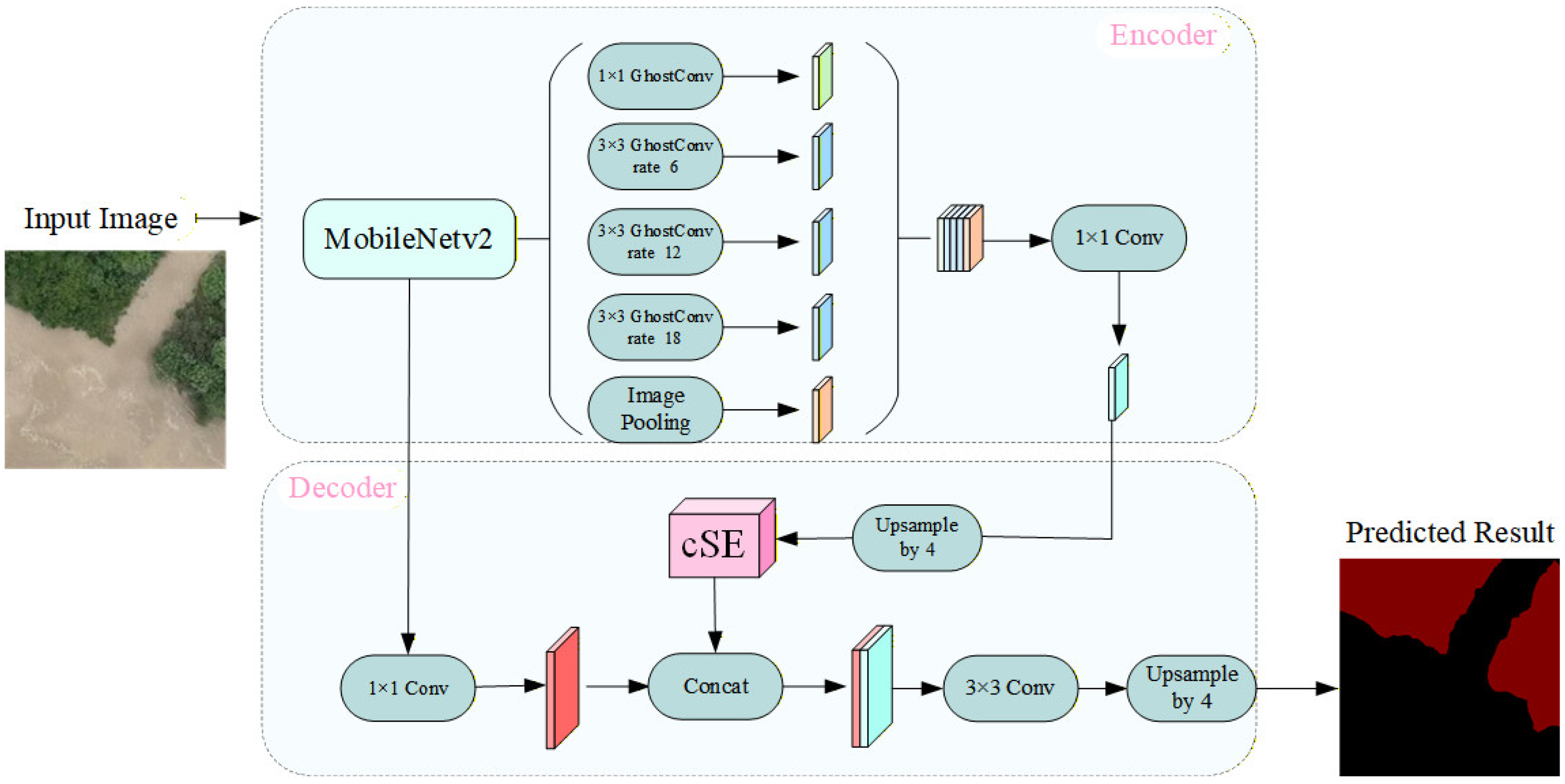
To address the limitations of the original DeepLabV3+ model in terms of high computational cost, insufficient feature discrimination, and redundancy in convolution operations, an improved lightweight DeepLabV3+ model is proposed in this study. The proposed model enhances feature segmentation capability while significantly reducing model complexity through three key modifications: the adoption of a lightweight backbone network, the introduction of a channel attention mechanism, and the optimization of convolution operations.

First, the original Xception backbone is replaced with MobileNetV2 to reduce the number of parameters and computational burden while maintaining effective feature segmentation capability. MobileNetV2 employs an inverted residual structure and linear bottleneck design, which improves feature propagation efficiency and alleviates the degradation problem in deep networks, making it more suitable for lightweight semantic segmentation tasks.

Second, a channel squeeze-and-excitation (cSE) attention module is introduced into the decoder stage to enhance the model’s ability to focus on informative feature channels. Specifically, one cSE module was inserted after the ASPP output feature was upsampled and before it was concatenated with the low-level feature. The cSE module was applied to the 256-channel high-level semantic feature, and the reduction ratio of the fully connected layers was set to 2, corresponding to a channel transformation of 256-128-256. By adaptively recalibrating channel-wise feature responses, the cSE module strengthens the representation of shrub-related features and suppresses background noise, which is particularly beneficial for distinguishing alpine shrubs from spectrally similar land cover types in complex environments.

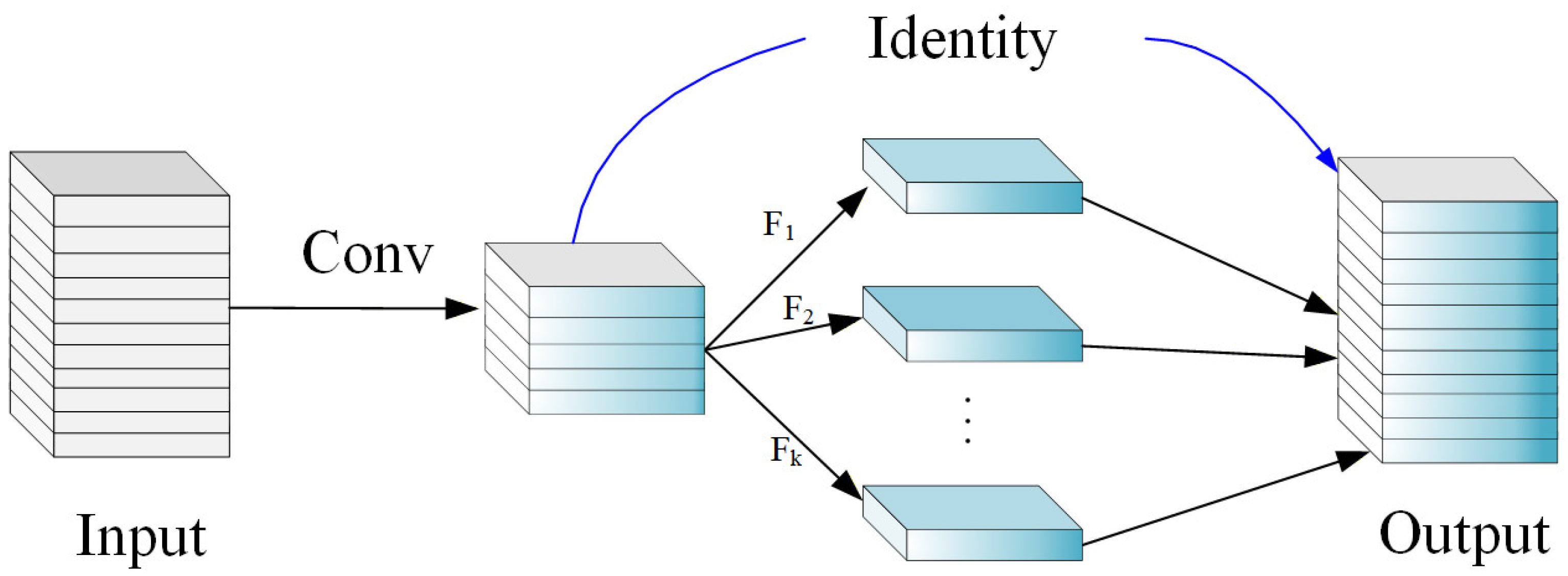
Third, to further reduce computational redundancy, standard atrous convolutions in the ASPP module are partially replaced with Ghost convolution. Ghost convolution generates additional feature maps through inexpensive linear operations based on a small number of intrinsic feature maps, thereby significantly reducing the number of parameters and floating-point operations (FLOPs) while preserving the representational capability of the network.

Through the integration of the above strategies, the proposed model achieves a better balance between segmentation accuracy and computational efficiency. The overall architecture of the improved DeepLabV3+ model is shown in Figure 6.

2.4.1. MobileNetV2 Backbone

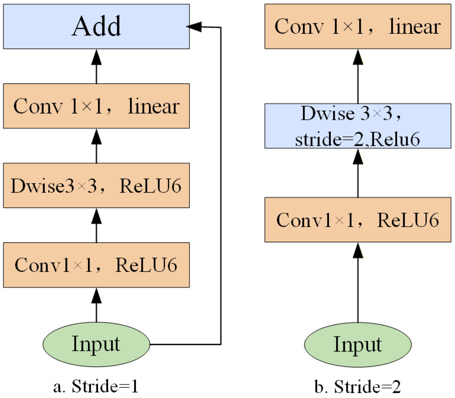
MobileNetV2 is a lightweight convolutional neural network proposed by Sandler et al. [16] designed for efficient computation and deployment in resource-constrained environments. In this study, MobileNetV2 is adopted to replace the original Xception backbone in DeepLabV3+ in order to reduce model complexity while maintaining effective feature segmentation capability. The network is built upon an inverted residual structure combined with a linear bottleneck design, in which the input features are first expanded using a 1 × 1 pointwise convolution, followed by a 3 × 3 depthwise separable convolution for spatial feature segmentation, and then projected back to a low-dimensional space through another 1 × 1 convolution. The structure of the inverted residual block is shown in Figure 7. When the input and output dimensions are consistent, a residual connection is introduced to facilitate feature reuse and improve information flow across layers. In addition, the use of linear activation in the bottleneck layer helps reduce information loss during dimensionality reduction. Owing to these structural advantages, MobileNetV2 significantly reduces the number of parameters and computational cost while maintaining competitive performance, making it well suited as a lightweight backbone for semantic segmentation tasks. Previous studies have achieved a good balance between the segmentation accuracy and computational efficiency of high-resolution drone images using an improved DeepLabV3+ framework based on MobileNetV2 [23].

2.4.2. cSE Channel Attention Mechanism

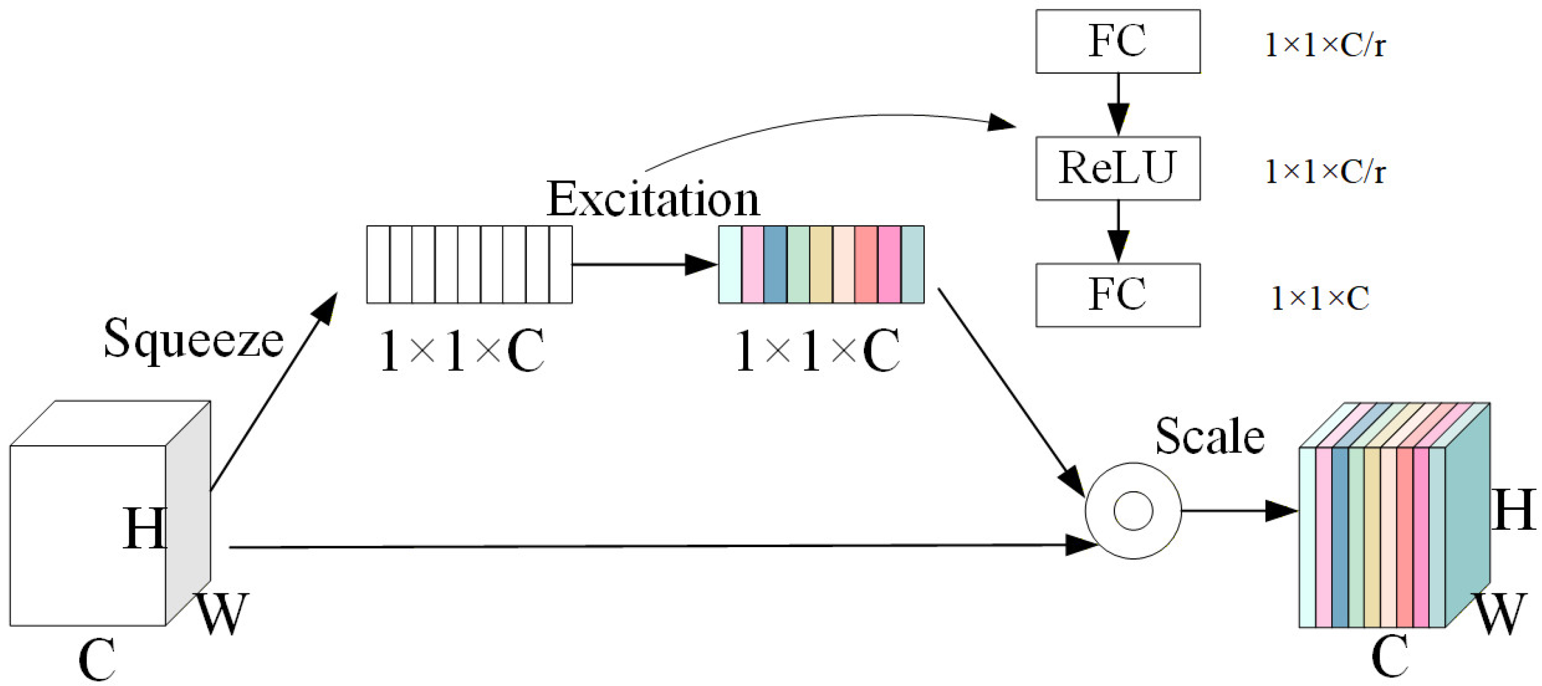
To enhance the model’s ability to capture discriminative features and suppress background noise, a channel squeeze-and-excitation (cSE) attention module is introduced into the decoder stage of the network. In the original DeepLabV3+ architecture, the use of atrous convolutions in the ASPP module enlarges the receptive field but may also lead to the loss of fine details and the introduction of redundant information. To address this issue, the cSE module is employed to recalibrate channel-wise feature responses before feature fusion, thereby improving the representation of informative features. As shown in Figure 8, the cSE module consists of three main operations: squeeze, excitation, and scale. First, global average pooling is applied to compress the spatial information of the input feature map into a channel descriptor, which captures global contextual information. Then, the descriptor is passed through two fully connected layers with a nonlinear activation function to learn channel-wise weights, followed by a sigmoid function to normalize the weights into the range of 0 to 1. Finally, the obtained weights are used to rescale the original feature map through channel-wise multiplication, which enhances important features and suppresses less relevant features [24]. By adaptively adjusting the importance of each channel, the cSE module improves the model’s ability to distinguish alpine shrubs from spectrally similar background objects, thereby enhancing segmentation accuracy in complex scenes.

2.4.3. Ghost Convolution (GhostConv)

Although the use of MobileNetV2 reduces model complexity at the backbone level, a large number of standard atrous convolution operations still remain in the ASPP module, resulting in considerable computational cost and redundant feature generation. To further improve computational efficiency, Ghost convolution (GhostConv) is introduced to replace part of the standard atrous convolutions in the ASPP module. GhostConv generates additional feature maps through inexpensive linear operations based on a small number of intrinsic feature maps, thereby reducing redundant computation while maintaining feature representation capability. Specifically, a small set of intrinsic feature maps is first obtained by standard convolution, and then a series of cheap linear transformations, such as depthwise convolutions, are applied to generate more feature maps, referred to as ghost features. The final output is formed by concatenating the intrinsic feature maps and the generated ghost feature maps. The structure of the GhostConv module is illustrated in Figure 9.

To further demonstrate the lightweight advantage of GhostConv, the numbers of parameters and floating-point operations (FLOPs) of standard convolution and GhostConv are theoretically compared under the same input setting. Assuming that the input feature map has a spatial size of $h\times w$, with $c$ input channels and $n$ output channels, and that the kernel size of standard convolution is $k\times k$, the numbers of parameters and FLOPs of standard convolution can be expressed by Equations (1) and (2), respectively.

$$p_{std}=k\times k\times c\times n$$

(1)

$$F_{std}=h\times w\times k\times k\times c\times n$$

(2)

For GhostConv, the output feature maps are generated in two stages, including intrinsic feature generation by standard convolution and ghost feature generation by cheap linear operations. The kernel size of these cheap linear operations is d × d. Accordingly, the numbers of parameters and FLOPs of these two parts can be calculated separately, and the total parameters and FLOPs of GhostConv are given by Equations (3) and (4).

$$p_{Ghc}=k\times k\times c\times {\displaystyle \frac{n}{s}}+d\times d\times (s-1)\times {\displaystyle \frac{n}{s}}$$

(3)

$$F_{Ghc}=h\times w\times k\times k\times c\times {\displaystyle \frac{n}{s}}+h\times w\times d\times d\times (s-1)\times {\displaystyle \frac{n}{s}}$$

(4)

Based on these derivations, the theoretical compression ratio and acceleration ratio of GhostConv relative to standard convolution can be obtained, as shown in Equations (5) and (6). Here, $R_p$ represents the theoretical compression ratio, and $R_F$ represents the theoretical acceleration ratio.

$$R_p={\displaystyle \frac{k\times k\times c\times n}{k\times k\times c\times \frac{n}{s}+d\times d\times (s-1)\times \frac{n}{s}}}\approx s$$

(5)

$$R_F={\displaystyle \frac{h\times w\times k\times k\times c\times n}{h\times w\times k\times k\times c\times \frac{n}{s}+h\times w\times d\times d\times (s-1)\times \frac{n}{s}}}\approx s$$

(6)

The results indicate that GhostConv requires substantially fewer parameters and FLOPs than standard convolution under the same input and output conditions. In particular, when $s>1$, both the theoretical compression ratio and acceleration ratio approach $s$, indicating that GhostConv can effectively reduce redundant computation while preserving comparable feature representation capability [22]. Therefore, introducing GhostConv into the ASPP module is beneficial for reducing model complexity and improving inference efficiency in alpine shrub segmentation tasks.

2.5. Experimental Environment and Parameter Settings

All experiments were conducted on a workstation running the Windows 11 operating system, equipped with an NVIDIA GeForce RTX 3050 GPU and 32 GB of RAM. The model was implemented and trained using the PyTorch deep learning framework, with Python 3.9, CUDA 11.8, and PyTorch 2.0.0.

The input image size was uniformly set to 256 × 256 pixels. To improve the reproducibility of the experiments, the random seed was set to 11. The total number of training epochs was set to 200, and the training process consisted of two stages: frozen training and unfrozen training. The batch size was set to 8 during the frozen training stage and 4 during the unfrozen training stage. The Adam optimizer was used for parameter optimization, with the exponential decay rates for the first- and second-moment estimates set to β1 = 0.9 and β2 = 0.999, respectively. The initial learning rate, minimum learning rate, and weight decay coefficient were set to 0.0007, 0.000007, and 0.0001, respectively. During training, the learning rate was dynamically adjusted using a cosine annealing strategy, and cross-entropy loss was adopted as the loss function. To monitor the training process, model performance was evaluated on the validation set every 10 epochs, and the corresponding model weights were saved.

The pretrained weight settings were specified separately for each model. For U-Net, the encoder was initialized using ImageNet-pretrained ResNet50 weights, while the decoder and task-specific segmentation layers were randomly initialized. For PSPNet, the matched layers were initialized using the pretrained PSPNet-MobileNetV2 weight file, while unmatched layers were randomly initialized. For SegNet, the encoder was initialized using ImageNet-pretrained VGG16-BN weights, while the decoder and task-specific segmentation layers were randomly initialized. For the proposed model, the matched layers were initialized using the pretrained DeepLabV3+-MobileNetV2 weights, while the newly introduced cSE module, GhostConv layers, and other unmatched layers were randomly initialized. This initialization strategy is commonly used in encoder–decoder semantic segmentation networks, where pretrained encoders provide general feature representations and newly added decoder or task-specific layers are randomly initialized [25,26].

2.6. Evaluation Metrics

To comprehensively evaluate the performance of the improved network model for alpine shrub segmentation, both segmentation accuracy and computational efficiency were considered. Segmentation accuracy was assessed using mean intersection over union (MIoU), mean pixel accuracy (mPA), F1-score, and overall accuracy (Accuracy), while computational efficiency was evaluated in terms of model size, number of parameters, and floating-point operations (FLOPs). In this study, segmentation performance metrics were calculated based on the confusion matrix, as shown in

Table 1. Confusion matrix.

Ground Truth	Predicted Value
	Positive Class	Negative Class
Positive Class	TP	FN
Negative Class	FP	TN

. In the confusion matrix, true positive (TP) denotes the number of pixels correctly predicted as the positive class, false negative (FN) denotes the number of positive pixels incorrectly predicted as the negative class, false positive (FP) denotes the number of negative pixels incorrectly predicted as the positive class, and true negative (TN) denotes the number of pixels correctly predicted as the negative class. In this binary segmentation task, shrub pixels were regarded as the positive class, whereas background and other non-shrub pixels were regarded as the negative class.

(1)

Mean intersection over union (MIoU) is a widely used evaluation metric in semantic segmentation tasks. It measures the ratio between the intersection and the union of the predicted shrub regions and the ground-truth regions, thereby providing an overall assessment of the model’s segmentation performance and robustness. The formulation of MIoU is given as follows:

$$MIoU={\displaystyle \frac{1}{N}}{\sum }_{i=0}^N{\displaystyle \frac{TP}{TP+FP+FN}}\times 100\%$$

(7)

(2)

Mean pixel accuracy (mPA) is an evaluation metric that measures the ratio of correctly classified pixels to the total number of pixels, thereby reflecting the pixel-level classification accuracy of the model. The formulation of mPA is given as follows:

$$mPA={\displaystyle \frac{1}{N}}{\sum }_{i=0}^N{\displaystyle \frac{TP}{TP+FP}}\times 100\%$$

(8)

(3)

The F1-score is defined as the harmonic mean of precision and recall, which provides a balanced consideration of these two metrics and offers a more comprehensive evaluation of the model’s classification performance. The formulation of the F1-score is given as follows:

$$F_1={\displaystyle \frac{2TP}{2TP+FN+FP}}$$

(9)

(4)

Accuracy represents the ratio of correctly predicted samples to the total number of samples, and its formulation is given as follows:

$$Accuracy={\displaystyle \frac{TP+TN}{TP+TN+FN+FP}}\times 100\%$$

(10)

(5)

Floating-point operations (FLOPs) refer to the number of floating-point operations required for a single forward pass of the model, and are mainly used to characterize the computational complexity of the model. In this study, the FLOPs of each model were calculated using the THOP library, with the input tensor size set to (1 × 3 × 256 × 256). Since convolution operations generally involve both multiplication and addition, both operations were counted as floating-point operations in this study. Therefore, the reported FLOPs values are twice the results calculated by THOP. In general, a higher FLOPs value indicates greater computational complexity and may lead to slower inference speed.

(6)

The number of parameters (Parameters) refers to the total number of trainable parameters in the model, which reflects the spatial complexity and storage requirement of the model. In this study, the number of parameters of each model was calculated using the THOP library under the input tensor size of (1 × 3 × 256 × 256). Generally, a larger number of parameters may increase the risk of overfitting and impose higher demands on computational resources and storage space.

In addition to the above segmentation accuracy metrics, three error-rate metrics were further used to evaluate the deviation in shrub area estimation and to distinguish different sources of segmentation errors. First, the relative shrub pixel error (RSE) was calculated to quantify the difference between the predicted shrub area and the ground-truth shrub area. This metric compares the number of shrub pixels predicted by the model with the number of shrub pixels in the ground-truth label and is defined as follows:

$$\mathrm{RSE}={\displaystyle \frac{\left|P_{\mathrm{shrub}}-G_{\mathrm{shrub}}\right|}{G_{\mathrm{shrub}}}}\times 100\%$$

(11)

where $P_{\mathrm{shrub}}$ represents the number of predicted shrub pixels and $G_{\mathrm{shrub}}$ represents the number of ground-truth shrub pixels. A lower RSE value indicates that the predicted shrub area is closer to the ground-truth shrub area. However, the relative shrub pixel error only reflects the overall difference in shrub pixel quantity and cannot distinguish whether the error is caused by missed shrub pixels or falsely detected shrub pixels. Therefore, the omission error rate and commission error rate were further calculated based on the pixel-level confusion matrix, as follows:

$$\mathrm{OER}={\displaystyle \frac{\mathrm{FN}}{\mathrm{TP}+\mathrm{FN}}}\times 100\%$$

(12)

$$\mathrm{CER}={\displaystyle \frac{\mathrm{FP}}{\mathrm{TP}+\mathrm{FP}}}\times 100\%$$

(13)

where (TP) represents correctly classified shrub pixels, FN represents shrub pixels incorrectly classified as background, and FP represents background pixels incorrectly classified as shrubs. The omission error rate represents the proportion of ground-truth shrub pixels missed by the model, while the commission error rate represents the proportion of predicted shrub pixels that actually belong to the background.

3. Results

3.1. Ablation Study of Improved DeepLabV3+ Model

To further evaluate the impact of the introduced MobileNetV2 backbone, cSE channel attention mechanism, and GhostConv on the performance of the improved model, ablation experiments were conducted in this study. Under the same dataset and experimental settings, the models were trained and validated, and the corresponding evaluation metrics were recorded for comparative analysis. The results of the ablation experiments are presented in

Table 2. Ablation results of improved DeepLabV3+ model under different module configurations.

Configuration	Backbone	cSE	Ghost Conv	MIoU/%	mPA/%	F1-Score/%	Accuracy/%	FLOPs	Parameters/M	Model Size/MB
1	Xception	×	×	84.94	90.29	88.84	92.83	41.71	54.71	209.27
2	MobileNetV2	×	×	85.63	91.01	89.49	93.12	13.22	5.81	22.45
3	MobileNetV2	√	×	88.07 ± 0.11	92.58 ± 0.18	91.51 ± 0.05	94.36 ± 0.02	13.22	5.88	22.70
4	MobileNetV2	√	√	88.47 ± 0.19	92.93 ± 0.18	91.80 ± 0.17	94.52 ± 0.09	12.15	3.79	14.75

Note: “√” indicates that the module was included, while “×” indicates that the module was not included. Values with ± indicate the mean ± standard deviation over three random seeds, namely 11, 22, and 42. FLOPs, parameters, and model size are architecture-dependent metrics.

.

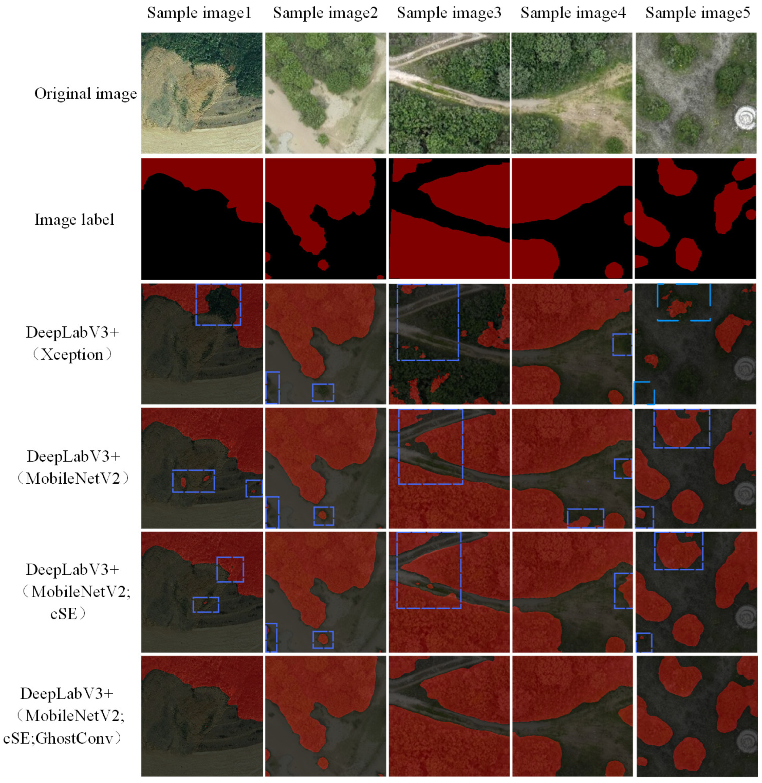
As shown in Table 2, compared with the original model, the proposed model improves MIoU, mPA, F1-score, and Accuracy by 3.53%, 2.64%, 2.96%, and 1.69%, respectively, indicating that the proposed improvements enhanced the segmentation performance for alpine shrub segmentation. When only the backbone network is replaced with MobileNetV2, the MIoU increases by 0.69%, while the number of parameters, FLOPs, and model size are significantly reduced, indicating that the lightweight backbone can effectively decrease model complexity while maintaining satisfactory feature segmentation capability. Furthermore, the key ablation experiments were further repeated using three random seeds to evaluate result stability. After introducing the cSE channel attention mechanism on the basis of the lightweight backbone, the average MIoU and mPA increase to 88.07 ± 0.11% and 92.58 ± 0.18%, respectively, demonstrating that the attention mechanism is effective for alpine shrub segmentation. This improvement can be attributed to the fact that alpine shrubs in UAV imagery often exhibit low contrast with background objects, fragmented boundaries, and irregular spatial distribution; the cSE module enhances shrub-related feature representation through channel-wise recalibration, thereby improving the model’s ability to identify both the main body and boundary details of alpine shrubs. After further incorporating GhostConv, the average MIoU, mPA and F1-score slightly increased to 88.47 ± 0.19%, 92.93 ± 0.18% and 91.80 ± 0.17%. The segmentation performance was slightly improved, whereas FLOPs, the number of parameters, and model size were reduced to 12.15, 3.79 M, and 14.75 MB, respectively. This indicates that GhostConv mainly contributes to reducing redundant convolution operations and model complexity while maintaining comparable segmentation performance. Overall, the lightweight backbone, cSE attention module, and GhostConv jointly improve the balance between segmentation accuracy and inference efficiency for alpine shrub segmentation. To further evaluate the contribution of each module, segmentation experiments were conducted on the validation set, and the results are shown in Figure 10.

As observed in Figure 10, the baseline DeepLabV3+ model demonstrates relatively poor segmentation performance, characterized by extensive missed detections and misclassifications. Specifically, it struggles to identify sparsely distributed shrubs, with the segmentation results exhibiting noticeable holes and jagged edges, which indicates insufficient attention to the boundary details of alpine shrubs. Upon replacing the backbone network with MobileNetV2, the segmentation performance improves, enabling the model to detect scattered shrubs with fewer misclassifications and omissions; however, challenges such as inaccurate boundaries and incomplete segmentation still remain. With the introduction of the cSE attention module, the model effectively alleviates the confusion between shrub features and background through channel-wise recalibration, leading to more accurate identification of small-scale shrubs and significantly reducing misclassification and omission. Ultimately, the proposed model achieves superior segmentation performance, characterized by smooth and continuous boundaries, with the segmentation results closely aligning with the ground truth.

3.2. Comparison of Segmentation Performance Among Different Models

To validate the effectiveness of the improved model for shrub segmentation, U-Net, PSPNet, DeepLabV3+ and SegNet were compared with the proposed DeepLabV3+ model on the validation set. The corresponding evaluation metrics are presented in

Table 3. Accuracy metrics of proposed method and comparative models.

Models	MIoU/%	mPA/%	F1-Score/%	Accuracy/%	FLOPs	Parameters/M	Model Size/M
U-Net	87.78	91.20	91.43	94.07	112.92	24.89	94.97
PSPNet	86.02	90.65	90.06	91.56	254.56	48.26	89.65
DeepLabV3+	84.94	90.29	88.84	92.83	41.711	54.71	209.27
SegNet	85.78	91.04	89.49	93.14	255.25	53.92	149.67
Proposed Method	88.47	92.93	91.80	94.52	12.15	3.79	14.75

.

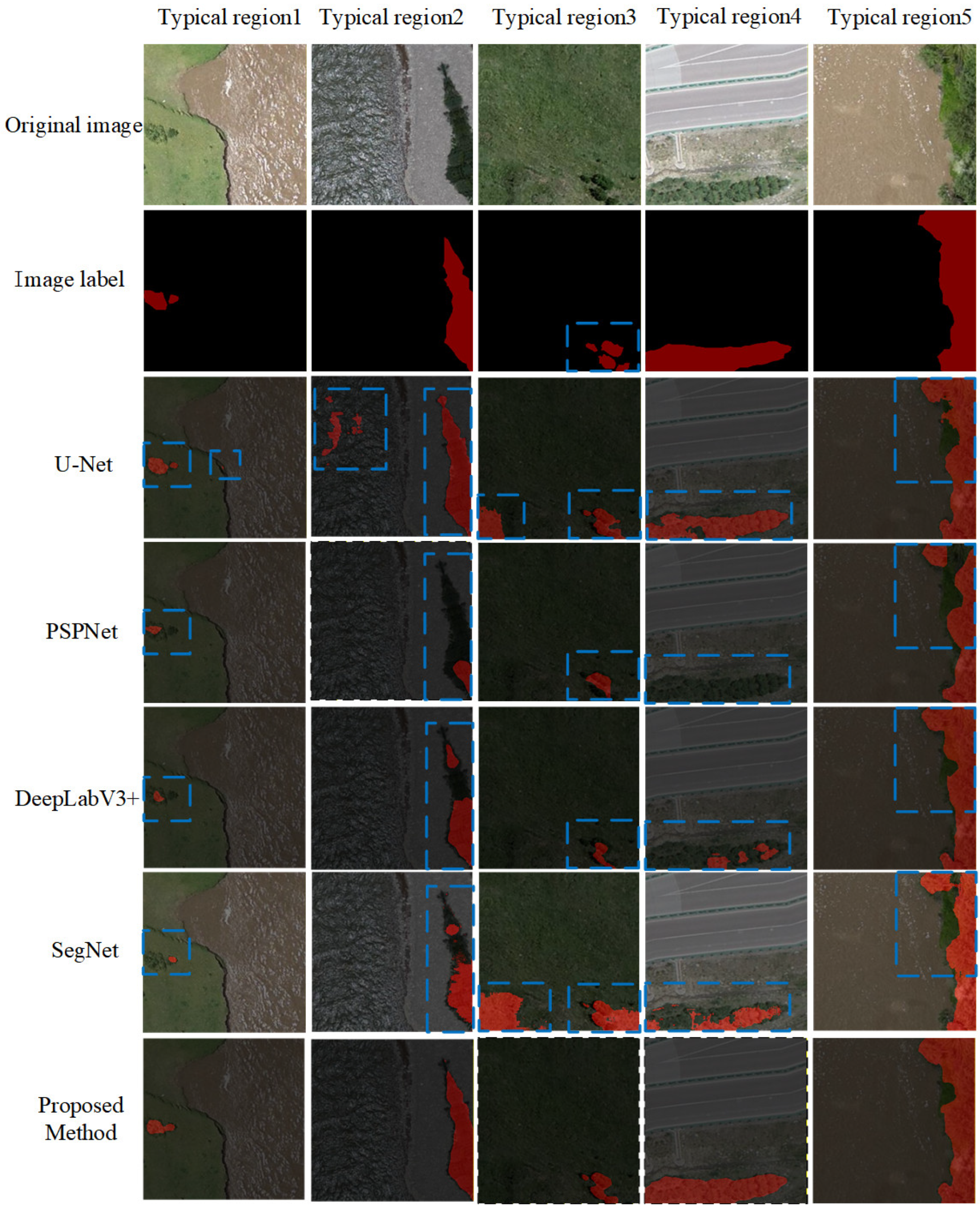
As shown in Table 3, the proposed model achieves superior segmentation performance compared with the other models while maintaining a more lightweight network structure. The U-Net model adopts a symmetric encoder–decoder architecture with skip connections and end-to-end training for image segmentation. Although it performs well in relatively simple scenarios, achieving MIoU and mPA of 87.78% and 91.20%, respectively, its performance deteriorates in complex backgrounds, such as mixed meadow and shrub environments, where feature segmentation becomes more challenging. PSPNet utilizes a pyramid pooling module to effectively capture and fuse multi-scale contextual information, thereby enhancing semantic understanding. However, its relatively high computational and space complexity leads to slower deployment, and the repeated downsampling operations reduce spatial resolution, resulting in the loss of fine details and causing extensive misclassification and omission in shrub segmentation tasks. DeepLabV3+ captures multi-scale features using atrous convolutions with different dilation rates; however, due to insufficient sampling density, part of the feature information may be lost during the segmentation process, leading to relatively lower accuracy and a large number of parameters. SegNet adopts an encoder–decoder structure and uses pooling indices to recover spatial information during upsampling, which can improve boundary restoration to some extent. However, in this study, SegNet still shows relatively high computational complexity, with FLOPs, parameters, and model size of 255.25, 53.92 M, and 149.67 M, respectively. In addition, its MIoU and F1-score are 85.78% and 89.49%, respectively, indicating that its segmentation accuracy and lightweight performance are still limited in complex alpine shrub scenes. In contrast, the proposed model achieves MIoU, mPA, and Accuracy of 88.47%, 92.93%, and 94.52%, respectively, demonstrating more precise boundary delineation and more complete segmentation of large shrub regions. Moreover, the computational burden is significantly reduced, owing to the optimized design that integrates high-quality feature segmentation with lightweight modules, allowing the model to maintain high segmentation accuracy while achieving efficient deployment performance. The segmentation results of different models in five typical regions are shown in Figure 11.

Through comparative analysis of the segmentation results, it can be observed that different models exhibit varying performance across the typical regions. For Regions 1 and 3, all models are able to identify sparsely distributed shrubs within large background areas, indicating that the main shrub features in these regions are relatively distinguishable. However, DeepLabV3+ and PSPNet mainly detect the central parts of shrubs and fail to accurately delineate the boundaries of scattered shrub patches. In contrast, the U-Net model is capable of capturing shrub boundaries to a certain extent due to its feature fusion mechanism, but its resistance to interference from spectrally similar objects, such as water bodies and meadows backgrounds, is relatively weak, resulting in some pixel-level misclassification. SegNet can identify part of the shrub regions by recovering spatial information through its encoder–decoder structure, but its segmentation results are still relatively fragmented, and omission errors occur in small or boundary-adjacent shrub patches. For Regions 2, 4, and 5, where the background is more complex and the spatial distribution of shrubs is more fragmented, all comparison models, including DeepLabV3+, U-Net, PSPNet, and SegNet, exhibit different degrees of misclassification and omission. Specifically, U-Net tends to produce false detections in complex background areas with similar spectral or textural characteristics, resulting in scattered misclassified shrub pixels. PSPNet shows relatively obvious omission in narrow and boundary-adjacent shrub regions, with incomplete segmentation of continuous shrub patches. DeepLabV3+ also suffers from omission errors in fragmented shrub areas, indicating its limited ability to preserve fine spatial details. SegNet can recover part of the shrub structure, but its segmentation results are still fragmented, with incomplete edge segmentation and discontinuous boundaries. In contrast, the proposed method achieves better shrub segmentation performance in shrub segmentation compared with the other models. Specifically, it produces more accurate and smoother boundaries, more complete segmentation of shrub regions, and more effective identification of sparsely distributed shrubs, demonstrating its advantage in handling complex segmentation scenarios.

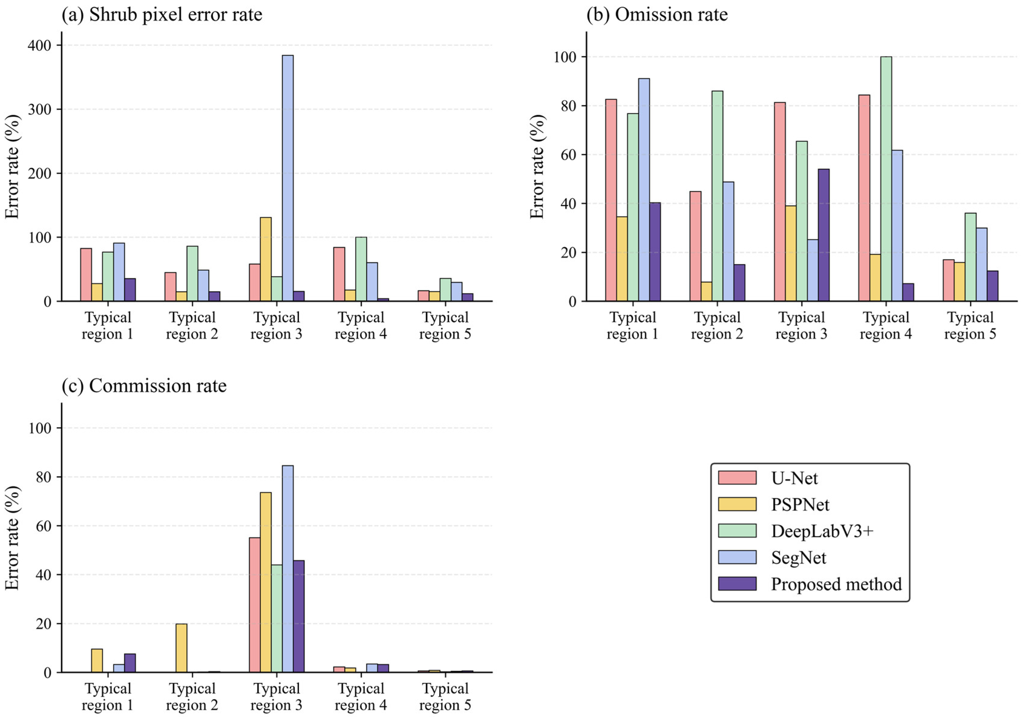
To further evaluate the area-level deviation and the sources of segmentation errors among different models, the relative shrub pixel error, omission error rate, and commission error rate were calculated according to the definitions described in Section 2.6. These metrics were used to quantify the overall difference between predicted and ground-truth shrub pixels and to distinguish missed shrub pixels from falsely detected shrub pixels. The corresponding results are shown in Figure 12.

As shown in Figure 12, the proposed method generally achieves lower shrub pixel error rates in most typical regions and showed more balanced performance in terms of omission and commission errors. Compared with U-Net, PSPNet, DeepLabV3+, and SegNet, the proposed method reduces obvious over-segmentation and under-segmentation in most complex shrub scenes. In particular, it maintains relatively low commission rates while reducing omission errors, indicating that the proposed method can more effectively distinguish shrub pixels from complex backgrounds.

3.3. Model Application in Real-World Scenarios

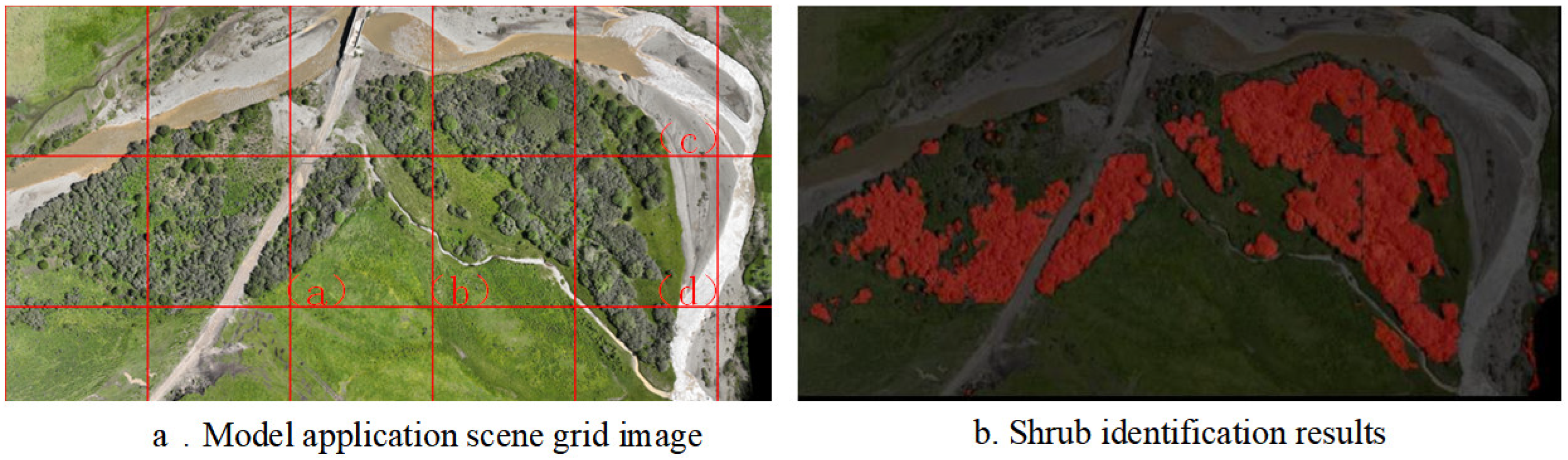
To further evaluate the applicability of the proposed model under similar UAV sensor and acquisition conditions, UAV imagery acquired in 2025 was selected for practical application. For this purpose, the original UAV images were uniformly cropped into numerous patches, each measuring 256 × 256 pixels. Regions smaller than 256 × 256 pixels were retained based on the remaining area. The application scenario and cropping process are illustrated in Figure 13a. Subsequently, the proposed model was employed to perform shrub segmentation on all cropped patches. After completing the segmentation of all patches, the predicted results were stitched together according to their original spatial positions to obtain the final global segmentation result for the test area, as shown in Figure 13b.

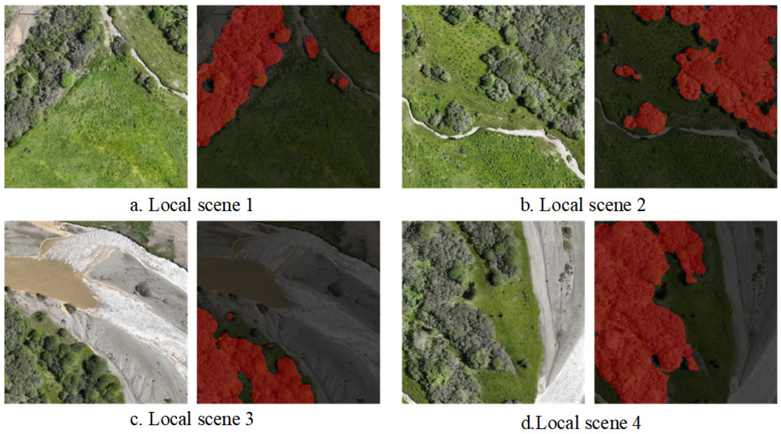
Figure 14 illustrates examples of selected image patches alongside their corresponding shrub segmentation results. As shown in the figure, the proposed model shows good performance in identifying shrub regions and delineating shrub boundaries within the selected UAV image patches. The validation results across these application scenarios indicate that the proposed model has potential applicability under similar UAV sensor and acquisition conditions. However, since these examples were derived from the same type of UAV imagery, further validation across diverse sites, seasons, and sensor platforms is still needed to more comprehensively evaluate the model’s generalization ability and robustness more comprehensively.

4. Discussion

It should be noted that the segmentation of alpine shrubs from UAV imagery remains a challenging task, and studies dedicated to their fine-scale identification are still limited. Unlike vegetation types with relatively continuous canopies, alpine shrubs are typically low in stature, patchily distributed, and characterized by irregular and discontinuous boundaries. In alpine environments, strong surface heterogeneity and the close interspersion of shrubs with grassland, bare soil, and gravel further increase the difficulty of accurate mapping, while the distinction between dwarf shrubs and surrounding vegetation is often unclear [27,28,29]. Moreover, previous studies have shown that shrubs in heterogeneous landscapes often exhibit high intra-class variability and low inter-class separability, making them difficult to delimit from surrounding vegetation and background features in high-resolution UAV imagery [30]. Accordingly, the central issue addressed in this study is not merely whether alpine shrubs can be segmented more accurately, but how a lightweight network can effectively capture fragmented spatial structures and weak discriminative features under highly heterogeneous alpine surface conditions. These challenges are also consistent with recent advances in remote sensing semantic segmentation. Recent methods such as MCCANet have emphasized the importance of multi-scale feature fusion and boundary supervision for preserving object boundaries in high-resolution remote sensing images [16]. SAM-DBNet and HyperR3SNet further indicate that stronger pretrained representations and vision foundation models can improve feature segmentation and generalization in complex remote sensing scenes [17,18]. Different from these more complex or foundation-model-based frameworks, this study focuses on a lightweight DeepLabV3+ architecture for UAV-based alpine shrub segmentation, aiming to improve the balance between segmentation accuracy and computational efficiency under fragmented and heterogeneous alpine surface conditions.

From a methodological perspective, the effectiveness of the proposed improvements can be interpreted in relation to the specific characteristics of alpine shrub target. MobileNetV2 provides an efficient feature segmentation scheme through inverted residuals and linear bottlenecks, which helps reduce model complexity while maintaining basic semantic representation capacity [20]. Similar lightweight replacement strategies have also been adopted in recent remote sensing and agricultural image segmentation studies to reduce computational cost while maintaining segmentation performance [31]. This is particularly important for UAV-based alpine shrub segmentation, because high-resolution UAV imagery contains abundant local details and often requires efficient processing for fine-scale vegetation mapping. The cSE module is particularly useful for alleviating spectral confusion between alpine shrubs and surrounding backgrounds. In alpine environments, shrub patches are often interspersed with grassland, bare soil, gravel, and shadowed areas, which may show similar spectral or textural responses in RGB imagery. By adaptively recalibrating channel-wise feature responses, the cSE module assigns higher weights to shrub-related channels and suppresses less informative or background-related channels, thereby strengthening the discriminative representation of shrub targets. Similar channel attention mechanisms have also been shown to improve feature discrimination in high-resolution remote sensing semantic segmentation by enhancing informative feature responses and reducing background interference [21,32]. Therefore, the cSE module helps the model distinguish fragmented shrub patches from spectrally similar backgrounds. Meanwhile, GhostConv reduces redundant feature generation through inexpensive linear operations, thereby decreasing computational cost while retaining useful feature information for segmentation [22]. Recent lightweight remote sensing segmentation studies have also introduced GhostNet or Ghost-like lightweight structures into DeepLabV3+-based frameworks to reduce model parameters and improve computational efficiency [33]. Within the DeepLabV3+ framework, the ASPP module further provides multi-scale contextual information, and the decoder helps recover spatial details and object boundaries [19]. Recent improved DeepLabV3+-based remote sensing segmentation models have similarly emphasized the importance of multi-scale feature segmentation for high-resolution imagery with complex backgrounds and small or fragmented targets [34]. Therefore, the improved network is not only lighter in architecture, but also more suitable for capturing the fragmented distribution, weak spectral separability, and irregular boundaries of alpine shrubs in heterogeneous UAV imagery.

Nevertheless, some limitations remain. As shown in the visual comparison and pixel-level error analysis, omission errors still occur in small, sparse, or boundary-adjacent shrub patches, while commission errors may appear in areas where grassland, bare soil, gravel, or shadowed backgrounds show spectral or textural similarity to shrubs. Some shrub–background transition zones also exhibit locally blurred or discontinuous boundaries. Similar difficulties have also been reported in UAV-based shrub and vegetation mapping studies conducted in heterogeneous landscapes [30]. In addition, the dataset used in this study was mainly collected from a single UAV platform and under relatively limited scene conditions. Therefore, the current results mainly reflect the applicability of the proposed model under similar UAV sensor and acquisition conditions, while its generalization ability across different sensors, regions, phenological stages, and illumination conditions still requires further verification.

Future work should further strengthen both dataset diversity and model adaptability. More samples acquired under different phenological stages, illumination conditions, terrain backgrounds, and alpine environments should be incorporated. At the data level, multi-source or multi-modal data fusion may further improve the discrimination of complex vegetation patterns [35,36]. At the model level, boundary-aware constraints, stronger multi-scale feature fusion, and more effective spatial interaction mechanisms may help reduce edge fragmentation and omission in complex scenes. In the longer term, lightweight and transferable UAV-based vegetation mapping frameworks may provide more practical support for ecological monitoring, habitat assessment, and alpine vegetation change studies [37].

5. Conclusions

This study presents an improved lightweight DeepLabV3+ model designed for the segmentation of alpine shrubs from high-resolution UAV imagery. The original Xception backbone was replaced with MobileNetV2, a channel squeeze-and-excitation (cSE) attention module was introduced into the decoder, and Ghost convolution was incorporated into the ASPP module. These modifications resulted in a more favorable balance between segmentation accuracy and computational efficiency within the dataset and experimental settings of this research. Compared to the original DeepLabV3+ model, the proposed method exhibited increases of 3.53%, 2.64%, 2.96%, and 1.69% in MIoU, mPA, F1-score, and Accuracy, respectively. Furthermore, the FLOPs, number of parameters, and model size were reduced to 12.15, 3.79 M, and 14.75 MB, respectively. When compared to U-Net, PSPNet, SegNet, and the original DeepLabV3+, the proposed method showed relatively better overall performance, achieving MIoU, mPA, F1-score, and accuracy values of 88.47%, 92.93%, 91.80%, and 94.52%, respectively. Additionally, UAV images acquired in 2025 were used as an independent cross-year validation dataset to assess the applicability of the proposed model under similar UAV sensor and acquisition conditions. The results suggest that the proposed method has good applicability for alpine shrub segmentation under similar data acquisition conditions. However, the validation data were still collected from the same UAV platform and covered relatively limited scene types. Therefore, the transferability and applicability of the proposed method across different sensors, regions, seasons, geomorphic backgrounds, and more complex real-world scenarios still require further verification.