


Highlights
What are the main findings?
- RAPS-UNet, a residual-attention U-Net coupled with a physics-constrained loss and confidence-weighted pseudo-label augmentation, achieves an RMSE of 0.20 m, an MAE of 0.16 m, and an R2 of 0.91 for tidal-flat DEM inversion against a field-surveyed reference, reducing field-validation RMSE by approximately 43% relative to the conventional inundation frequency–elevation linear model.
- A four-level validation protocol—covering in-distribution validation, spatial holdout testing, and field-based assessment over interpolation (RMSE = 0.17 m) and extrapolation (RMSE = 0.22 m) zones—demonstrates that the proposed model retains accuracy beyond the spatial footprint of clustered ICESat-2 tracks, where residual learning, attention-based multi-source fusion, physics-constrained loss, and pseudo-label augmentation together address feature heterogeneity, physical consistency, and label sparsity.
What are the implications of the main findings?
- The proposed framework provides a practical approach to high-precision DEM retrieval over small-scale tidal flats (~1 km2 in spatial extent) where ICESat-2 elevation labels are sparse and spatially clustered, directly supporting fine-scale coastal monitoring, geomorphic change analysis, and intertidal ecological assessment.
- By coupling physics-constrained learning with confidence-weighted pseudo-label augmentation, the study extends supervised deep learning beyond its conventional dependence on dense, well-distributed labels, offering a potentially adaptable framework for remote-sensing inversion in other observation-sparse coastal and geomorphological settings.
Abstract
High-precision topography of tidal flats is essential for coastal monitoring, geomorphic change analysis, and ecological assessment. Although satellite remote sensing supports repeated and large-area observation, topographic inversion over small-scale tidal flats—here defined as localized intertidal patches with limited areal extent, represented in this study by a 1.11 km2 tidal flat near Dafeng Port—remains challenging, because ICESat-2 laser altimetry tracks across such areas are typically sparse and spatially clustered within narrow sub-regions, leaving extensive observation-blind zones without direct elevation labels. This label-clustering problem constrains the applicability of traditional empirical models and tends to cause deep learning models to generalize poorly beyond the spatial distribution of training samples. To address this issue, this study proposes a Residual Attention Physical-constraint Semi-supervised U-Net (RAPS-UNet) that fuses ICESat-2 ATL03/ATL08 elevation labels with Sentinel-1 SAR and Sentinel-2 optical features. The preprocessing pipeline comprises refined ICESat-2 photon filtering, adaptive inundation-frequency extraction, multi-source feature selection, and baseline DEM construction. RAPS-UNet integrates residual learning, attention-based multi-source fusion, physics-constrained loss, and confidence-weighted pseudo-label augmentation to improve extrapolation under clustered-label conditions. A four-level validation protocol—in-distribution validation, spatial holdout testing, and field-based assessment over both interpolation and extrapolation zones—was designed to evaluate spatial generalization. Against a field-surveyed DEM, RAPS-UNet achieved an overall RMSE of 0.20 m, an MAE of 0.16 m, and an R2 of 0.91; the field-based interpolation and extrapolation zones yielded RMSEs of 0.17 m and 0.22 m, respectively, while the spatial holdout test reached an RMSE of 0.23 m and an R2 of 0.81. Relative to the traditional inundation frequency–elevation linear model (RMSE = 0.35 m), RAPS-UNet reduced the field-validation RMSE by approximately 43%. The proposed framework therefore offers a practical approach for fine-scale coastal-zone topographic mapping under sparse and spatially clustered altimetry conditions.
1. Introduction
Tidal flats are dynamic land–sea transitional zones that provide ecological protection, carbon sequestration, and coastal defense functions [1,2,3]. High-precision tidal-flat topography is essential for coastal monitoring and hazard assessment, but field and vessel-based surveys are costly and temporally limited [4,5,6]. Satellite remote sensing provides an efficient alternative for repeated tidal-flat topographic monitoring. Optical spectral indices are effective for surface-water and wetland feature extraction [7,8,9,10], while SAR observations provide complementary all-weather information [11,12].
Building on multi-source remote sensing, tidal-flat topographic inversion methods have gradually evolved from empirical approaches toward data-driven modeling. Traditional methods such as the waterline method and the inundation frequency method have been widely applied to tidal-flat topographic reconstruction [13,14]. However, their reliance on simplified elevation–water relationships limits their ability to capture the complex spatial variability of tidal-flat morphology. Machine learning approaches improve nonlinear feature modeling capability but still depend heavily on handcrafted features [15]. More recently, deep learning methods have enabled end-to-end feature learning and spatial-context modeling, achieving promising performance in tidal-flat mapping and topographic inversion [16,17].
Across this evolution, the supervisory signal underlying topographic inversion has remained dependent on limited high-precision elevation references, making the choice of altimetric platform critical. Spaceborne laser altimetry has therefore become an important data source for coastal topographic reconstruction. The Global Ecosystem Dynamics Investigation (GEDI) provides full-waveform LiDAR observations that have been applied to land-surface elevation retrieval [18], whereas ICESat-2 offers photon-counting laser altimetry with higher spatial sampling density and has become increasingly adopted in coastal applications [19]. Subsequent studies have integrated ICESat-2 observations with Sentinel imagery for nearshore bathymetric mapping and shallow-water topographic reconstruction [20,21]. Since Xu et al. [22] first combined ICESat-2 altimetry with Sentinel-2-derived inundation frequency features for tidal-flat topographic inversion, the “ICESat-2 + multi-source remote sensing” paradigm has been widely adopted and further extended to multiple tidal-flat environments [23,24]. However, most existing studies implicitly assume that ICESat-2 observations are sufficiently dense and spatially distributed to support supervised learning [22,23,24]. While this assumption is often valid at regional scales, it may not hold for small-scale tidal flats, where only a limited number of ICESat-2 ground-track segments intersect the study area and are frequently concentrated within a narrow sub-region. Under such label-clustered conditions, large portions of the tidal flat may remain unsampled, reducing the effectiveness of both empirical and fully supervised learning approaches and creating substantial challenges for reliable spatial extrapolation [25]. Traditional empirical models (e.g., waterline and inundation-frequency methods) cannot fully exploit multi-source remote sensing features, while conventional fully supervised learning suffers from poor spatial generalization under incomplete label coverage. Addressing this challenge requires mechanisms that extend the supervisory signal beyond directly observed labels while maintaining physically plausible predictions in unlabeled regions.
Semi-supervised learning (SSL) has been widely adopted to alleviate label scarcity by exploiting unlabeled samples. Representative SSL strategies include pseudo-label self-training [26], consistency-regularization frameworks such as Mean Teacher and FixMatch [27,28], and their variants, which have been extensively reviewed in both the machine-learning and remote-sensing communities [29]. These approaches generally construct additional supervisory signals from unlabeled data and thereby improve model generalization under limited-label conditions. The strategy adopted in this study differs from canonical SSL. Rather than iteratively generating pseudo-labels from the model’s own predictions, soft labels are derived from a baseline DEM and distance-based propagation of hard ICESat-2 labels, with confidence weights assigned according to label provenance. Under the taxonomy of Zhou [30], this scheme is conceptually closer to weak supervision combined with label propagation. Nevertheless, because the framework jointly optimizes labeled and unlabeled pixels within a unified learning process, the term “semi-supervised” is retained throughout this study. The implementation details and methodological distinction are further described in Section 3.1.1.
A second complementary research direction incorporates prior physical knowledge into the learning process to improve reliability beyond the support of training data, commonly referred to as physics-informed or physics-guided machine learning. The seminal physics-informed neural network (PINN) framework incorporates governing partial differential equations as soft constraints on network outputs [31], and subsequent studies have extended this concept across a wide range of scientific applications [32]. Recent reviews classify these approaches along a spectrum from hard-constrained formulations based on explicit governing equations to physics-guided models that encode domain knowledge through architectural design or loss-level priors without solving a specific physical equation [33,34]. The present study belongs to the latter category. Rather than solving governing equations or imposing hard physical constraints, prior geomorphological knowledge is incorporated through physics-constrained loss terms, including residual-range constraints relative to a baseline DEM and topographic smoothness regularization (Section 3.1.2). This positioning is consistent with the broader view that integrating process understanding into data-driven Earth system models can improve robustness in data-sparse environments [35], which directly aligns with the small-scale tidal flat inversion scenario considered here.
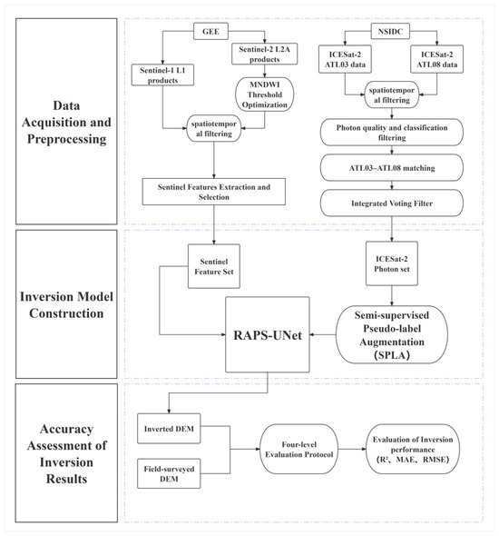
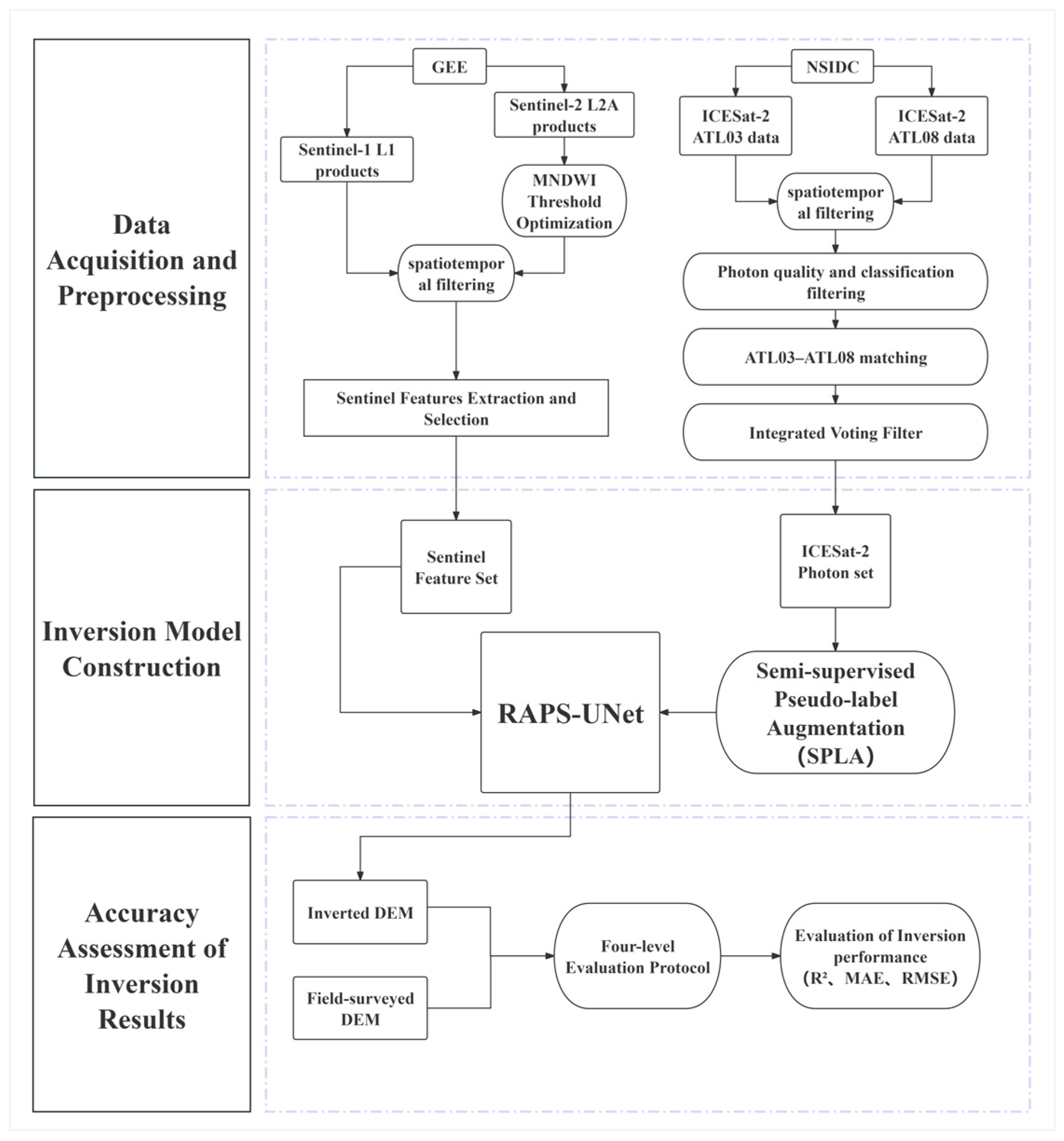
To address this gap, the present study focuses on small-scale tidal flats under label-clustered ICESat-2 observation conditions, where large portions of the study area lack direct elevation supervision. Under this setting, conventional fully supervised inversion suffers from poor spatial generalization, while empirical methods remain limited in their ability to exploit heterogeneous multi-source remote sensing features. To overcome these limitations, we propose the Residual Attention Physical-constraint Semi-supervised U-Net (RAPS-UNet), which integrates residual learning, attention mechanisms, physics-constrained loss, and confidence-weighted pseudo-label augmentation to improve extrapolation capability and prediction reliability in unlabeled regions. The model is applied to the small-scale tidal flat surrounding Dafeng Port, Yancheng, and evaluated against an independent field-surveyed DEM. The overall technical workflow is shown in Figure 1.
Figure 1.
Technology roadmap.
2. Study Area
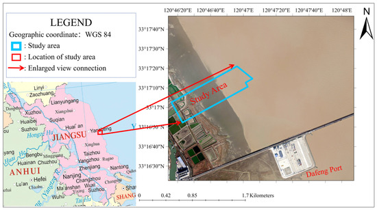
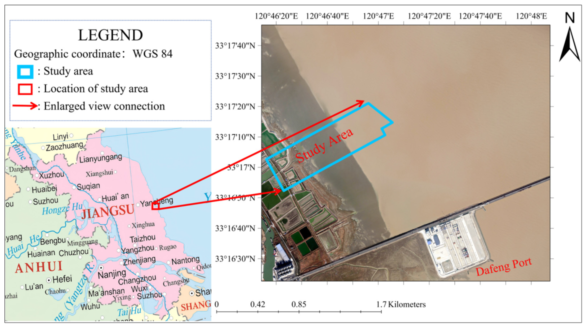
The study area selected for this research is a localized tidal flat covering approximately 1.11 km2 in the vicinity of Dafeng Port, Yancheng City, Jiangsu Province, China (120°46′15.6942″E–120°47′06.0760″E, 33°16′52.1929″N–33°17′21.2113″N), as shown in Figure 2. The area includes nearshore zones, intertidal flats, subtidal zones, and limited permanently inundated water bodies. It is characterized by a silt-clay coastal environment with highly turbid waters, typical of the Yellow Sea coastal system. The regional tidal regime is regular semi-diurnal. The site is additionally influenced by ongoing coastal engineering and human activities, resulting in dynamic shoreline erosion–accretion transitions [36]. This localized tidal flat was selected as a representative small-scale study site because the available ICESat-2 ground tracks are spatially clustered along one side of the area, leaving substantial regions without direct elevation observations and thereby posing a challenging topographic extrapolation problem.
Figure 2.
Schematic map of study area. Caption: The red box in the figure indicates the location only and does not represent the actual size of the study area.
3. Methods and Experimental Design
This section describes the complete methodological framework of the study. It begins with the acquisition and preprocessing of multi-source datasets, including ICESat-2 altimetry, Sentinel remote sensing imagery, and field-surveyed DEM data. It then introduces the proposed RAPS-UNet framework, covering pseudo-label generation, model architecture, and comparative experiment design. Finally, the evaluation protocol and quantitative metrics adopted to assess interpolation and extrapolation performance are presented.
3.1. Data Acquisition and Preprocessing
This subsection describes the acquisition of the multi-source datasets used in this study and the preprocessing procedures applied to generate reliable elevation labels and remote sensing input features for subsequent model training and validation.
3.1.1. ICESat-2 and Sentinel Data Acquisition
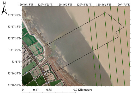
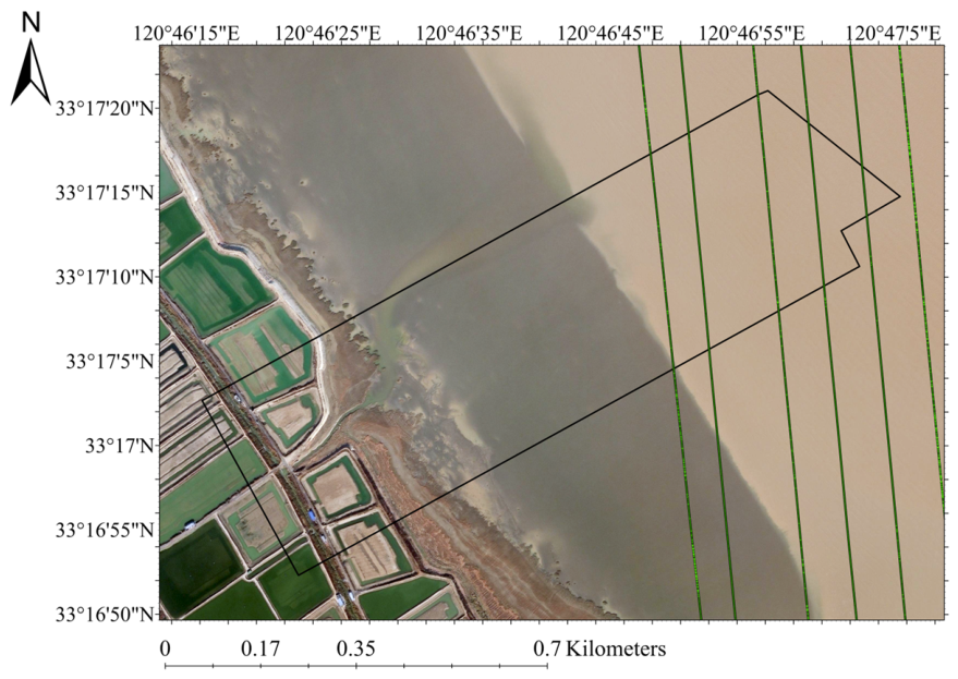
This study used the ATL03 Global Geolocated Photon Data and ATL08 Land and Vegetation Height products from the ICESat-2 satellite, publicly released by the National Snow and Ice Data Center (NSIDC) [37,38]. The acquisition period spanned January 2020 to January 2025. ATL03 provides photon-level geographic coordinates, WGS-84 ellipsoidal heights (h_ph), and signal confidence values, while ATL08 provides classification flags for ATL03 photons that support preliminary signal screening. Photons satisfying signal_conf_ph = 4 and classed_PC_flag = 1 were retained, and ATL03 photons were matched with ATL08 classifications through timestamp correspondence. After spatial filtering, three ICESat-2 ground tracks intersecting the study area were retained (Figure 3). These tracks were spatially clustered along one side of the study area, leaving substantial regions without direct elevation observations.
Figure 3.
ICESat-2 Photon Trajectory in study area (from left to right ATL03-20210220142019-gt1lr, ATL03-20200223074100-gt1lr, ATL03-20200822230035-gt1lr). Caption: The black box in the figure indicates the extent of the study area.
To generate stable multi-source remote sensing features, Sentinel imagery was collected over a broader temporal window from January 2019 to January 2022. Sentinel-1 SAR imagery was obtained from the Ground Range Detected (GRD) dataset provided by the European Space Agency (ESA, Paris, France) and accessed via Google Earth Engine (Google LLC, Mountain View, CA, USA) (Level-1, IW mode, VV/VH dual polarization; 165 scenes). Sentinel-2 optical imagery was obtained from the Copernicus Sentinel-2 Level-2A Surface Reflectance Harmonized dataset provided by the European Space Agency (ESA, Paris, France) and accessed via Google Earth Engine (Google LLC, Mountain View, CA, USA) (cloud cover < 10%; 50 scenes). All imagery was resampled to a uniform spatial resolution of 10 m for subsequent feature extraction.
3.1.2. ICESat-2 Photon Refined Filtering
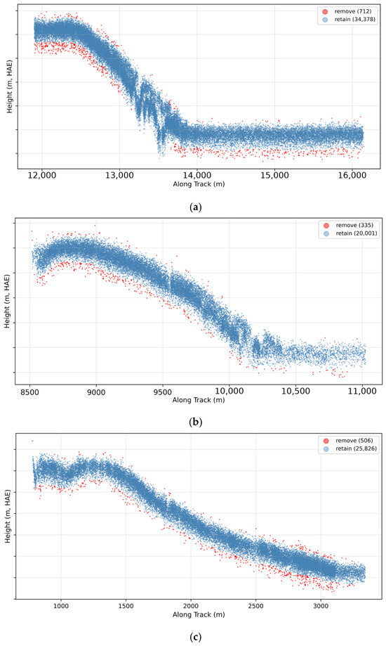
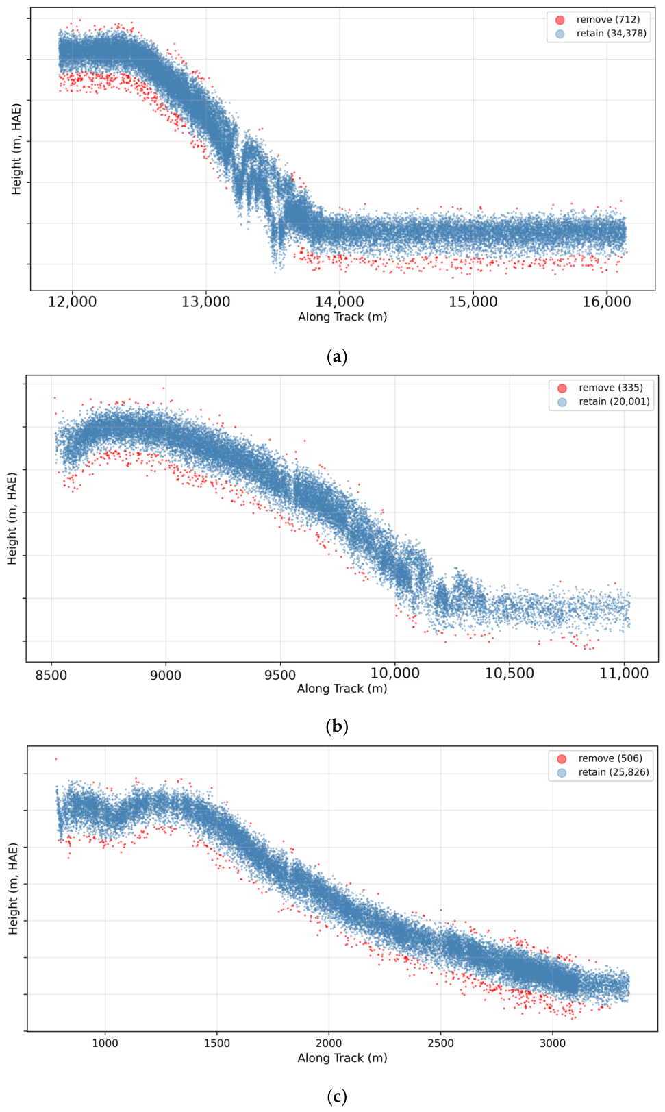
Following the initial screening based on photon confidence and classification flags, a small number of elevation outliers may still persist in the preliminary-filtered ICESat-2 dataset. To further suppress residual noise, an Integrated Voting Filter (IVF) framework was applied, combining three complementary methods: Adaptive Elliptical Filtering (AEF), a local sliding-window IQR method, and DBSCAN spatial clustering. These methods target anomalous photons from three complementary perspectives, namely along-track trend consistency, local statistical distribution, and three-dimensional spatial density. Photon points identified as noise by two or more methods were removed. This voting strategy improves filtering robustness while reducing the risk of excessive rejection of valid signal photons.
3.1.3. Remote Sensing Feature Extraction and Selection
The Modified Normalized Difference Water Index (MNDWI) enables scene-by-scene binary segmentation of imagery into water and non-water regions, and is calculated as follows:
where Green denotes the reflectance of the green band and SWIR denotes the reflectance of the shortwave infrared band. Conventional studies typically adopt MNDWI > 0 as the water body classification threshold [39]; however, this threshold was established based on clear urban water bodies. In the high-sediment-load turbid water conditions of the present study area, SWIR reflectance is substantially elevated [40], leading to a systematic underestimation of inundation frequency. Furthermore, prior research has noted that a fixed uniform threshold exhibits inherent limitations across varying water body conditions [41]; although threshold optimization methods such as Otsu’s method can partially alleviate this issue, their optimal performance is highly dependent on the characteristics of the grayscale histogram distribution [42,43]. Accordingly, an information-score-based threshold optimization method is proposed. By iterating over 11 candidate threshold values spanning [0.0, 1.0], the pixel-level inundation frequency of Sentinel-2 time-series imagery is computed for each threshold, and its mean, standard deviation, minimum, and maximum are statistically characterized. These statistics are then input into a scoring function to select the optimal threshold, formulated as follows:
where is the mean and is the standard deviation. The scoring function favors a uniform distribution of inundation frequency, to which the highest weight is assigned; the standard deviation and range terms each account for 30%, jointly measuring information richness from dispersion and extreme gradient. Based on the optimal threshold, seven categories of candidate features were extracted (Table 1), including optical water indices, SAR backscatter and texture descriptors, inundation-frequency-related variables, and spatial-context features that have been widely adopted in tidal-flat topographic inversion and remote sensing studies. The corresponding datasets, indices, and feature-construction methods are summarized in Table 1 together with their references. Subsequently, variance-based filtering was applied to remove features with a normalized standard deviation below 0.01, followed by correlation clustering to eliminate redundancy. Feature pairs with |r| > 0.85 were grouped into redundant clusters, from which only the feature showing the highest correlation with the elevation labels was retained. The resulting feature set was then used as the input to the model.
Table 1.
Sentinel feature set.
3.1.4. Field-Surveyed DEM for Independent Validation
The field-surveyed DEM used for independent validation was acquired in November 2024, with a spatial resolution of approximately 0.45 m. The DEM was referenced to the WGS-84/UTM Zone 51N horizontal coordinate system and the WGS-84 ellipsoidal vertical datum, consistent with the ICESat-2, Sentinel-1, and Sentinel-2 datasets. Therefore, no additional coordinate transformation was required. This dataset was used exclusively for independent accuracy assessment and was not involved in model training, pseudo-label generation, or parameter tuning. For quantitative comparison, the field-surveyed DEM was resampled to the spatial resolution of the inversion outputs and further partitioned into interpolation and extrapolation zones based on spatial proximity to the ICESat-2 observation footprint.
3.2. RAPS-UNet Model and Experimental Design
This section presents the proposed RAPS-UNet framework, the comparative experimental design, and the evaluation methodology used in this study. First, the construction of the RAPS-UNet model is described, including the hierarchical pseudo-label augmentation strategy and the network architecture. Next, comparative experiments based on the traditional inundation frequency–elevation linear model and ablation variants are designed to evaluate the contribution of the proposed components. Finally, a four-level evaluation protocol together with quantitative accuracy metrics is introduced to systematically assess both interpolation performance within observed regions and extrapolation capability beyond the ICESat-2 observation footprint.
3.2.1. Construction of the RAPS-UNet Model
The construction of the proposed RAPS-UNet framework consists of two components: a hierarchical pseudo-label augmentation strategy designed to extend supervision beyond the limited ICESat-2 observation footprint, and the network architecture for multi-source topographic inversion.
Hierarchical Pseudo-Label Augmentation Strategy
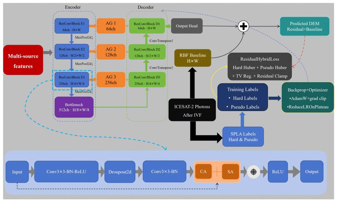
Since virtually all ICESat-2 photon trajectories passing through the study area are concentrated on one side (Figure 4), certain regions lack elevation labels entirely. Under a fully supervised paradigm, deep learning models inevitably degenerate in unlabeled regions into regressing toward the mean of training samples from the densely observed zone. Accordingly, drawing on the pseudo-label self-training strategy in remote sensing [55], a hierarchical semi-supervised pseudo-label augmentation strategy is proposed to extend the supervised region from the ICESat-2 trajectory-covered portion to all valid pixels.
Figure 4.
Architecture of the RAPS-UNet model.
Within the augmentation strategy, labels are assigned to four tiers in descending order of confidence. The first tier comprises hard labels derived from re-filtered ICESat-2 data and carries the highest weight. The second tier generates propagation labels by applying inverse distance weighting interpolation within a 5-pixel neighborhood of the hard labels; these carry lower weight than the hard labels and serve to smooth the supervisory transition between hard labels and pseudo-labels. The third tier assigns baseline DEM values as pseudo-labels to unlabeled pixels that approach or exceed the observational limits of ICESat-2, with weights that decay exponentially as a function of distance from the known observation zone, providing weak guidance along the direction of the elevation gradient. The fourth tier applies baseline DEM values as extremely low-weight global constraints to all remaining valid pixels, preventing the model from generating physically implausible predictions in entirely unsupervised regions.
RAPS-UNet Architecture
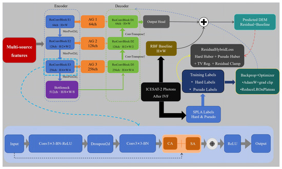
The architecture of the Residual Attention Physical-constraint Semi-supervised U-Net (RAPS-UNet) is illustrated in Figure 4.
RAPS-UNet adopts an encoder–decoder fully convolutional architecture incorporating residual convolutional blocks (ResConvBlocks), convolutional block attention modules (CBAM), attention gates (AG), and a physics-constrained composite loss function. The model predicts an elevation residual field relative to a baseline DEM rather than directly estimating absolute elevation values. The prediction target is defined as:
where denotes the elevation residual field, and is the baseline DEM generated from ICESat-2 observations. The final predicted elevation is then synthesized from and :
where is the residual prediction output by the network. The baseline DEM was generated from the re-filtered ICESat-2 elevations using radial basis function (RBF) interpolation followed by Gaussian low-pass filtering. Residual labels were then calculated by subtracting the baseline DEM from the observed elevations and used as the training target. This “baseline elevation field + residual correction” inversion paradigm has been demonstrated to be effective in multi-source data fusion inversion [56]. The network receives a multi-source feature tensor of size C × H × W and outputs a residual elevation map at the same spatial resolution. The encoder consists of three resolution-decreasing residual convolutional blocks (ResConvBlocks) connected in series with a bottleneck layer, with progressive down-sampling performed through max pooling at each stage. Each ResConvBlock employs residual connections [57] and embeds a Convolutional Block Attention Module (CBAM) [58] to adaptively enhance feature channels correlated with elevation and to focus on spatial regions exhibiting pronounced topographic variation.
In tidal flat scenarios, encoder features affected by turbid water bodies contain substantial background texture and spectral noise; direct concatenation into the decoding pathway may therefore introduce interference. To address this, an Attention Gate (AG) [59] is placed at each of the three skip connections, using the decoder output as a gating signal to conditionally filter encoder features and suppress noise irrelevant to elevation prediction. The decoder progressively restores spatial resolution through three stages of transposed convolution, each of which also embeds a CBAM. At the output end, two convolutional layers form a prediction head that outputs the elevation residual. The final elevation synthesis is expressed as:
where denotes the set of all valid raster pixels.
The loss function design of this model follows the principle of incorporating physical knowledge into deep learning to enhance prediction reliability [35], and references the technical framework in which physical equations are introduced as constraint terms in the loss function [31]. Beyond the data-driven fitting objective, spatial plausibility constraints are incorporated to form the physics-constrained composite loss function, expressed as follows:
where is the Huber loss over the hard-label region, with the residual target as the supervisory signal, used to handle residual coarse-error photons remaining after re-filtering. is the weighted Huber loss over the pseudo-label region:
where is the set of pseudo-labeled pixels excluding the validation set, is the confidence weight assigned to each tier, and is the pseudo-label residual value at the corresponding position. The coefficient is set to 0.5 to prevent the contribution of the pseudo-label supervisory signal from exceeding that of the true labels, thereby avoiding model overfitting to low-confidence pseudo-supervision.
is the total variation smoothness regularization term:
where is the associated weight. This term penalizes high-frequency spatial oscillations in the residual prediction field, preventing prediction artifacts from emerging in transition regions with sparse labels.
is the residual physical bounding term, which penalizes predictions that exceed a physically reasonable residual range:
This term directly encodes prior geographic knowledge (the expected deviation between tidal flat topography and the baseline DEM) into the loss function, constraining the extrapolation behavior of the model in unsupervised regions and imposing physical bounds on the predicted outputs.
The model was optimized using AdamW with an initial learning rate of 1 × 10⁻³ and a weight decay of 1 × 10⁻⁴. An adaptive learning-rate scheduling strategy, ReduceLROnPlateau, was applied according to the RMSE of the random in-distribution validation set (Val). Gradient clipping was employed to prevent gradient explosion caused by the total variation and residual clamp terms during the early stages of training. The maximum number of training epochs was set to 500, and early stopping was triggered when the Val RMSE showed no improvement for 80 consecutive epochs.
3.2.2. Comparative Experiment Design
Comparative experiments were designed to evaluate both the overall inversion performance of RAPS-UNet and the contribution of its individual components. Specifically, a traditional inundation frequency–elevation linear fitting model was used as an external baseline, while ablation experiments were conducted as internal comparisons.
For the baseline comparison, the re-filtered ICESat-2 elevations were spatially aligned with the inundation frequency raster derived using the optimal MNDWI threshold. Photon elevations within each pixel were aggregated using the median, and only pixels containing at least three photon events were retained to ensure robust regression. A linear relationship between inundation frequency and elevation was then established and applied to generate the corresponding inversion result, which was subsequently evaluated against the field-surveyed DEM.
For internal comparison, an ablation experiment comprising six model variants was designed to assess the contribution of the four core components of RAPS-UNet: residual learning (R), attention mechanisms (A), physics-constrained loss (P), and pseudo-label augmentation (S). The attention component includes CBAM-based channel/spatial attention within the residual blocks and Attention Gate spatial filtering in the decoder, while the physics-constrained component includes total variation smoothness regularization and residual amplitude clamping. Each ablation variant removes one component while retaining the remaining three, with a baseline U-Net containing none of the four components serving as the lower-bound reference. All variants were trained using identical training/validation splits, hyperparameter settings, and random seeds to ensure fair comparison.
3.2.3. Evaluation Protocol
Due to the strong spatial clustering of ICESat-2 labels in the eastern portion of the study area (Section 3.1.1; Figure 3), conventional random splitting cannot adequately evaluate model behavior in the unobserved western region. We therefore designed four mutually exclusive evaluation subsets (Table 2) to separately assess in-distribution fitting and spatial extrapolation performance.
Table 2.
Definition of the four evaluation subsets used in the accuracy assessment.
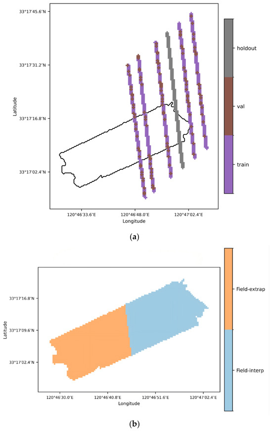
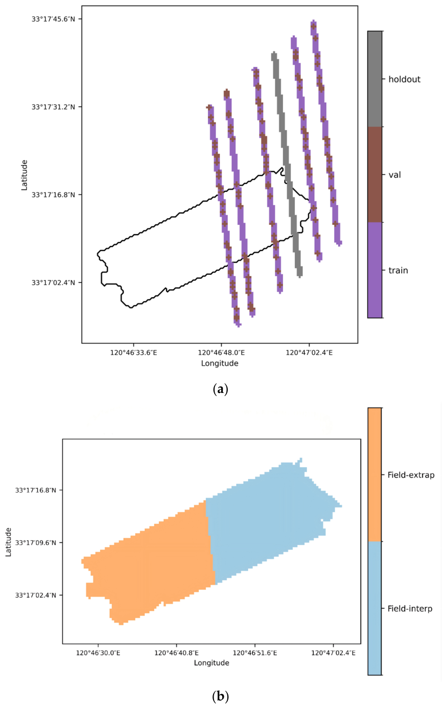
Figure 5 illustrates the spatial distribution of the four evaluation subsets used in this study. The ICESat-2 labels were divided into training, validation, and spatial hold-out subsets, where the hold-out subset was completely excluded from model training and pseudo-label generation (Figure 5a). The field-surveyed DEM was further partitioned into interpolation and extrapolation zones according to the distance to the nearest ICESat-2 label, with a threshold of 100 m. This design enables the evaluation framework to assess both label-space generalization and field-based extrapolation performance (Figure 5b).
Figure 5.
Spatial distribution of the evaluation subsets: (a) ICESat-2 label split for training, validation, and spatial hold-out testing; (b) field-surveyed DEM zones for interpolation and extrapolation evaluation based on the distance to the nearest ICESat-2 label. Caption: The black box in the figure delineates the boundary of the field-surveyed data within the study area.
The Val subset was used only for convergence monitoring and hyperparameter tuning, whereas the Holdout strip was fully excluded from training, baseline DEM construction, and pseudo-label generation to test label-side extrapolation. The field-surveyed DEM was divided into Field-interp and Field-extrap zones using a 100 m distance threshold from the nearest training-eligible ICESat-2 label, approximately corresponding to the strong–weak beam-pair spacing of ICESat-2. Together, Holdout and Field-extrap provide complementary evaluations of label-space and field-based extrapolation.
3.2.4. Accuracy Assessment
During accuracy assessment, the field-surveyed DEM was resampled to match the spatial resolution of the inversion outputs, enabling cell-to-cell comparison with the predicted topography. Model performance was quantified using the root mean square error (RMSE), mean absolute error (MAE) and coefficient of determination (R2), calculated as follows:
where denotes the inverted elevation value of the i-th pixel; denotes the in situ measured elevation value of the i-th pixel; represents the mean value of all in situ measured elevations; and is the total number of pixels included in the assessment. These metrics were consistently applied across the validation, holdout, field-interpolation, and field-extrapolation subsets.
4. Results
This section presents in sequence the results of water body threshold optimization, ICESat-2 photon refined filtering, inundation frequency–elevation model fitting and inversion, RAPS-UNet inversion, and RAPS-UNet ablation experiments. This section also includes a direct comparison between the RAPS-UNet inversion results and those of the traditional inundation frequency–elevation linear model.
4.1. Water Body Threshold Optimization Results
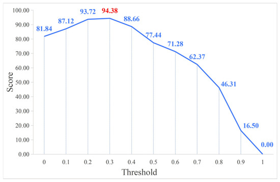
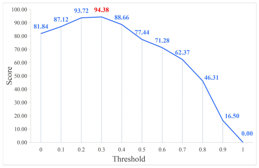
By applying the adaptive threshold optimization algorithm to 50 scenes of Sentinel-2 time-series imagery, 11 candidate thresholds spanning [0.0, 1.0] were evaluated. The pixel-level inundation frequency statistics and the corresponding scoring results are summarized in Table 3, and the score curve across all candidate thresholds is shown in Figure 5.
Table 3.
Optimal Threshold of MNDWI. Caption: The bold value indicates the highest score and the selected optimal threshold.
As shown in Figure 6, the score curve exhibits a clear single-peak structure, rising from 81.84 at threshold 0.0 to a maximum of 94.38 at threshold 0.3, and subsequently declining monotonically as the threshold increases further. Thresholds of 0.2 and 0.3 yield comparable scores (93.72 and 94.38), but threshold 0.3 is preferred because its inundation frequency mean (0.47) is closer to the ideal value of 0.5, indicating a more balanced water–land classification across the time series. The resulting optimal threshold (0.3) is substantially higher than the conventional fixed threshold of 0, reflecting the positive shift in SWIR reflectance caused by the enhanced scattering of high-turbidity water in the study area.
Figure 6.
Score curve of MNDWI threshold optimization. Caption: The red number indicates the highest score.
4.2. ICESat-2 Photon Refined Filtering Results
The preliminary-filtered ICESat-2 photon dataset was subjected to integrated voting refined filtering to further remove elevation outliers. The filtering results are presented in Figure 7a–c.
Figure 7.
ICESat-2 Integrated Voting Filter results: (a) ATL03-20210220142019-gt1lr, (b) ATL03-20200223074100-gt1lr, (c) ATL03-20200822230035-gt1lr.
4.3. Inundation Frequency–Elevation Model Fitting and Inversion Results
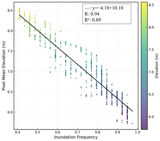
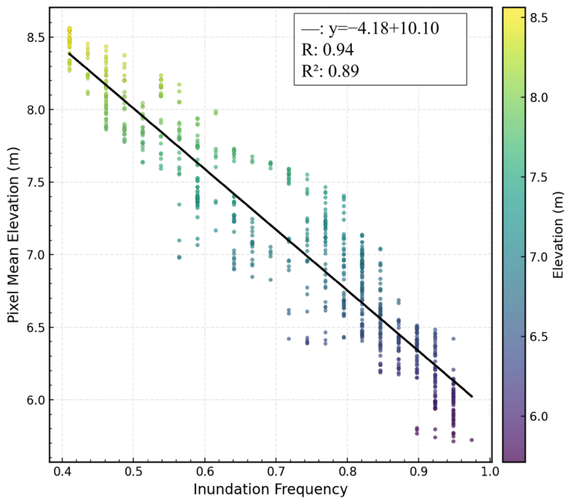
By statistically characterizing the pixel-level inundation frequency and corresponding elevation values within the study area, the fitted inundation frequency–elevation linear model is:
where y is the pixel elevation and x is the corresponding pixel inundation frequency. The linear fitting model achieves a Pearson correlation coefficient R of 0.94 and R2 of 0.89. The correspondence between elevation and inundation frequency is shown in Figure 8.
Figure 8.
Inundation frequency–Elevation Linear Regression.
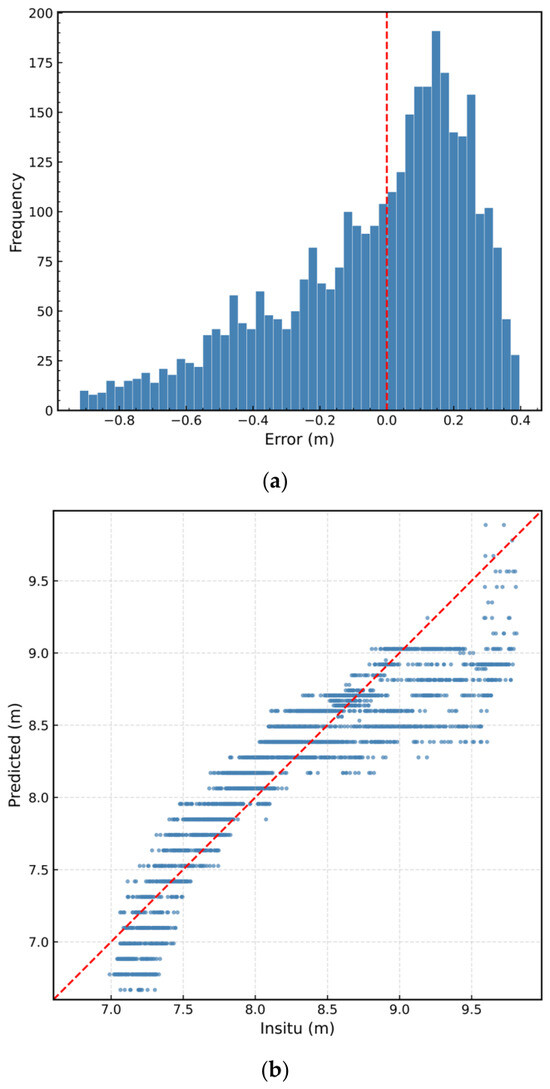
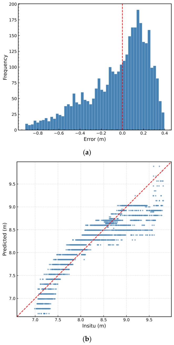
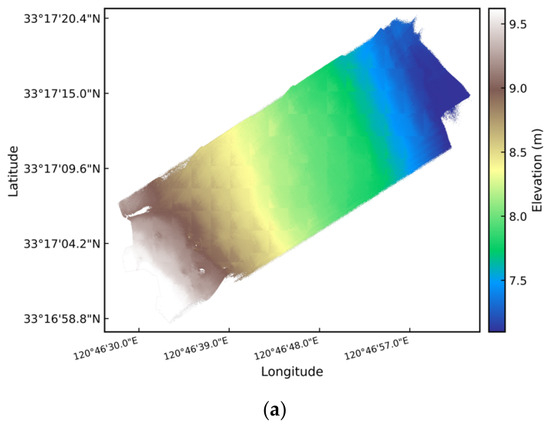
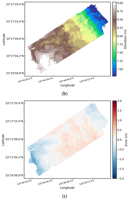
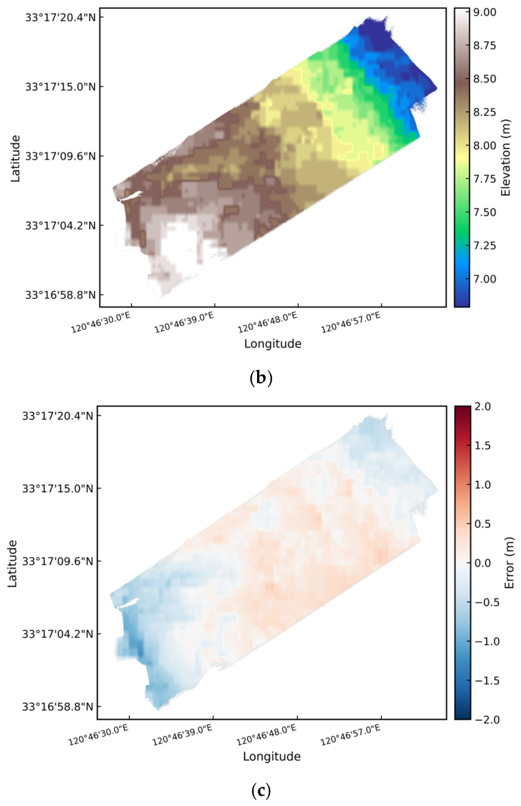
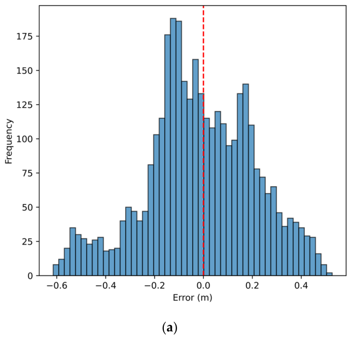
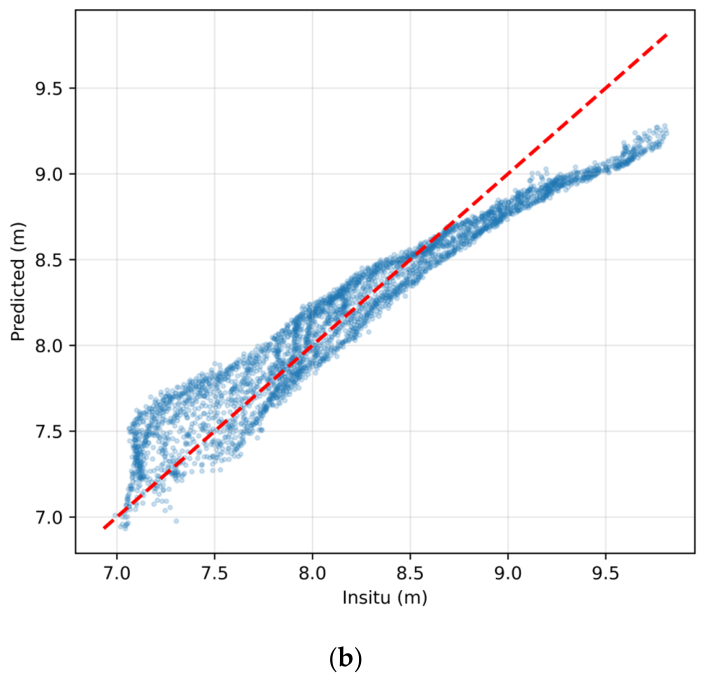
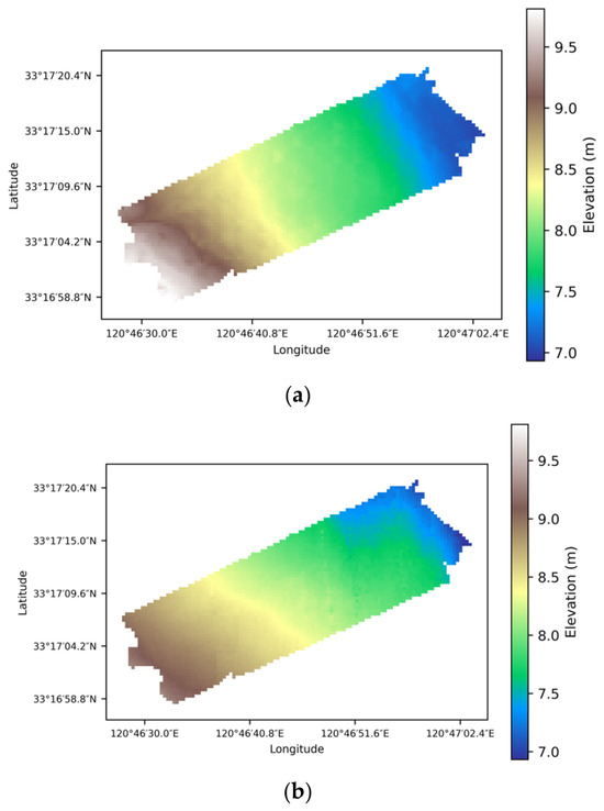
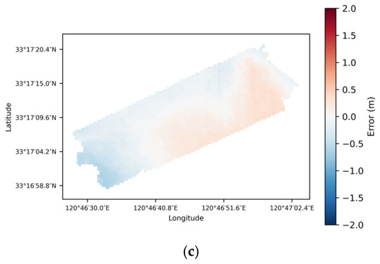
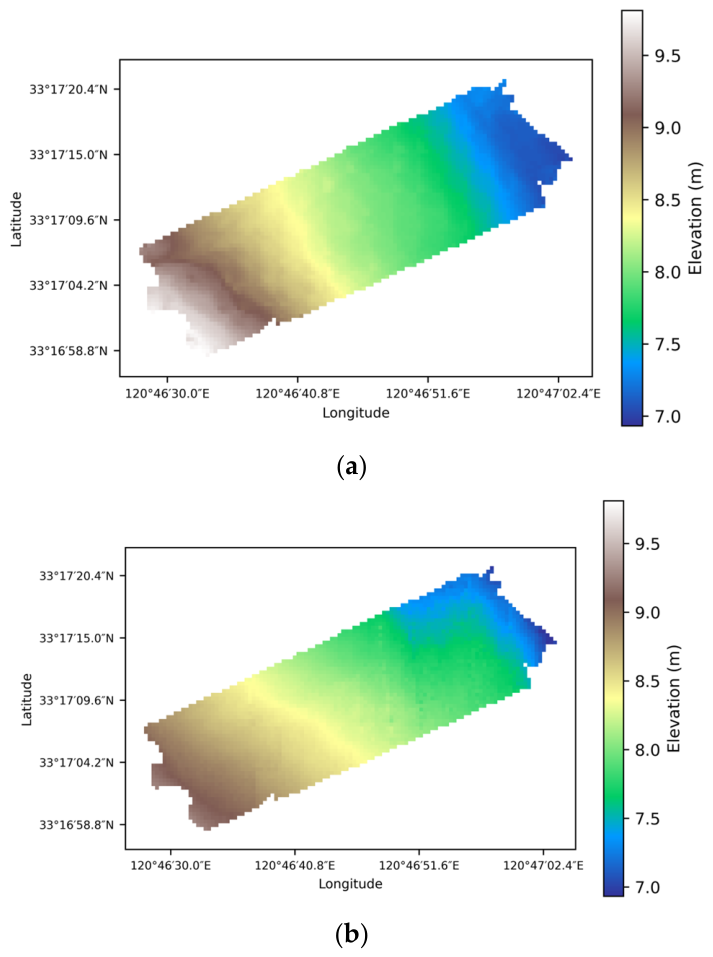
The traditional inundation frequency–elevation linear model yielded an RMSE of 0.35 m, MAE of 0.25 m, and R2 of 0.80 over the overlapping area with the field-surveyed DEM (Table 4). The error histogram (Figure 9a) exhibits a broad and asymmetric distribution, with errors spanning approximately −0.9 m to 0.4 m and a pronounced negative tail. This indicates that the inundation frequency–elevation model produces substantial local errors and tends to underestimate elevation in part of the study area. In the consistency scatter plot (Figure 9b), the predicted values show a distinct stepped pattern rather than a continuous distribution, reflecting the discretized nature of the inundation-frequency representation. Deviations from the 1:1 line are particularly evident at both ends of the elevation range, with overestimation in the lower-elevation range and underestimation in the higher-elevation range. Although the predicted DEM (Figure 10b) reproduces the general southwest-to-northeast elevation gradient of the study area, the spatial error map (Figure 10c) reveals evident systematic bias and contiguous error regions.
Table 4.
Inversion Results of the Inundation Frequency–Elevation Linear Fitting Model.
Figure 9.
Error and correlation analysis for the inundation frequency–elevation linear model inversion: (a) histogram of error distribution, (b) scatter plot of consistency.
Figure 10.
Evaluation of inundation frequency–elevation linear model inversion results: (a) field-surveyed DEM, (b) inverted DEM, (c) spatial distribution map of errors between field-surveyed and inverted results.
The relatively poorer performance of the inundation frequency–elevation model is mainly attributable to its reliance on a single inundation descriptor, which cannot fully capture the complex spatial variability of tidal-flat topography in small-scale regions. In addition, local water-classification uncertainty and the limited dynamic range of inundation frequency within the study area further amplify prediction errors, particularly in regions lacking strong elevation contrast.
4.4. RAPS-UNet Inversion Results
Over the full overlapping area between the inverted DEM and the independent field-surveyed DEM, RAPS-UNet achieved an overall RMSE of 0.20 m, MAE of 0.16 m, and R2 of 0.91 (Table 5). Compared with the traditional inundation frequency–elevation baseline reported in Section 4.3, the RMSE was reduced from 0.35 m to 0.20 m, corresponding to an approximately 43% reduction in RMSE. These results indicate that the proposed framework successfully reconstructed the large-scale topographic pattern of the study area despite the spatially clustered distribution of ICESat-2 labels.
Table 5.
Overall Inversion Results of RAPS-UNet.
To further distinguish interpolation from extrapolation performance, the field-surveyed DEM was partitioned into Field-interp and Field-extrap subsets according to the evaluation protocol described in Section 3.2.3. In the near-label region (Field-interp), RAPS-UNet achieved an RMSE of 0.17 m, MAE of 0.14 m, and R2 of 0.73. In the far-label region (Field-extrap), the RMSE and MAE increased moderately to 0.22 m and 0.18 m respectively, while R2 remained comparable at 0.74 (Table 6). The increase in absolute error indicates that prediction uncertainty gradually increases with distance from the ICESat-2 observation domain, reflecting the intrinsic difficulty of spatial extrapolation under label-sparse conditions. Nevertheless, the extrapolation-region RMSE (0.22 m) remained substantially lower than the overall RMSE of the traditional inundation frequency–elevation linear model (0.35 m), indicating that RAPS-UNet retained stable topographic reconstruction capability even in regions lacking direct ICESat-2 supervision.
Table 6.
Field-interp and Field-extrap inversion Results of RAPS-Unet.
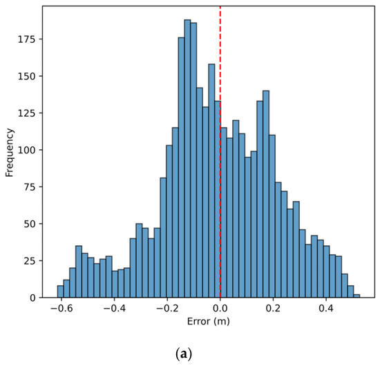
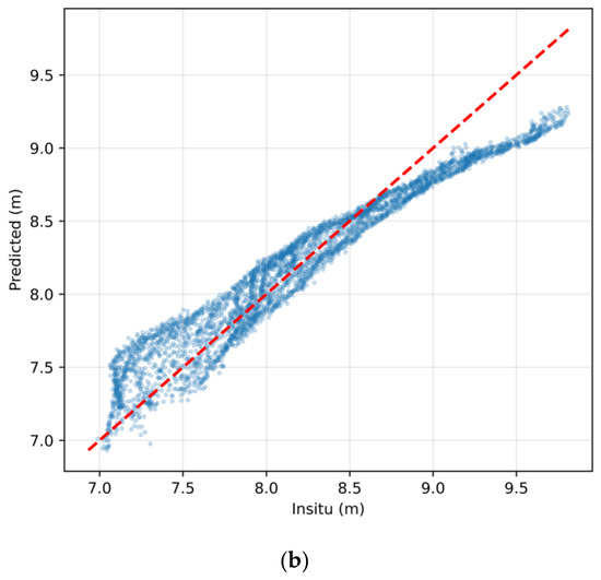
The error histogram (Figure 11a) shows that the inversion errors follow an approximately normal distribution centred near zero, with a slight negative tail indicating localized underestimation. In the field-surveyed versus predicted scatter plot (Figure 11b), most samples are distributed closely along the 1:1 line across the full elevation range, with no pronounced outliers or large-scale prediction collapse observed.
Figure 11.
Error and correlation analysis for RAPS-UNet: (a) histogram of error distribution, (b) scatter plot of consistency.
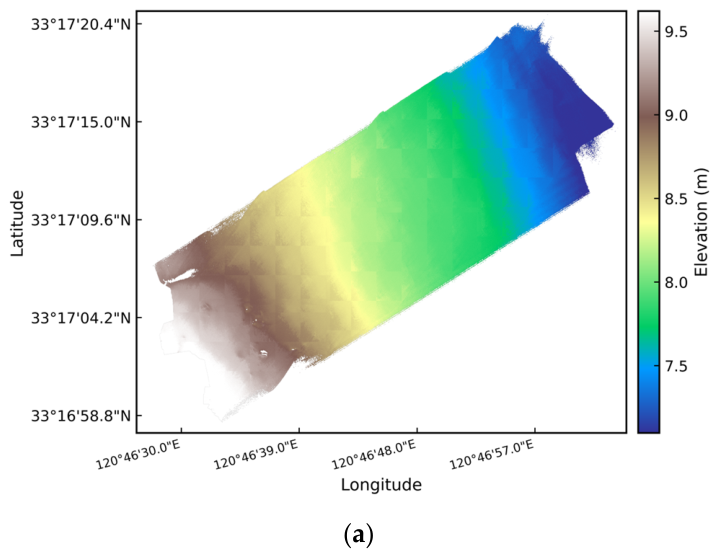
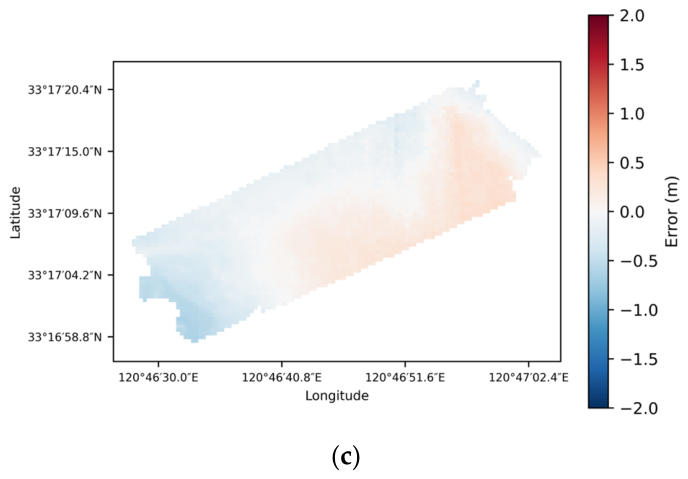
The predicted DEM (Figure 12b) is highly consistent with the field-surveyed DEM (Figure 12a) in terms of the overall spatial elevation pattern, successfully reproducing the southwest-to-northeast topographic gradient of the study area. The spatial error distribution (Figure 12c) further indicates that most regions exhibit relatively small inversion errors, while moderate systematic deviations remain in portions of the far-label region.
Figure 12.
Evaluation of RAPS-UNet inversion results: (a) field-surveyed DEM, (b) inverted DEM, (c) spatial distribution map of errors between field-surveyed and inverted results.
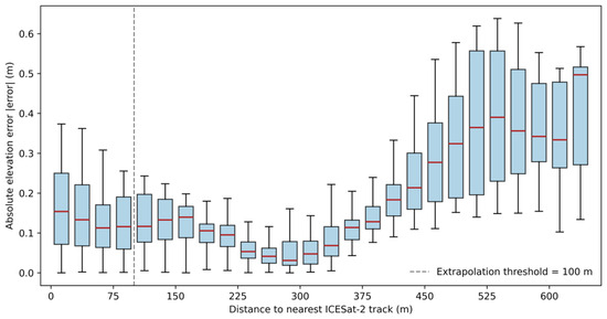
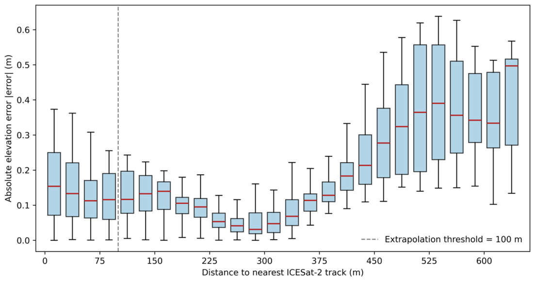
Absolute error did not increase monotonically with distance from ICESat-2 tracks (Figure 13), but showed a U-shaped pattern. Errors were moderate near the tracks, lowest at intermediate distances, and increased substantially beyond approximately 300 m, indicating the onset of genuine spatial extrapolation. The near-track errors may reflect residual photon-height noise, local geolocation uncertainty, and scale mismatch, whereas far-label errors mainly reflect the reduced constraint from elevation anchors.
Figure 13.
Absolute Error vs. Distance to Nearest ICESat-2 Track (Boxplot). Caption: Boxes indicate the interquartile range (IQR), red horizontal lines indicate the median absolute error, and whiskers represent the 1.5 × IQR. The dashed grey line marks the 100 m extrapolation threshold defined in Section 3.2.3.
Compared with previous ICESat-2-based tidal-flat studies conducted under broader or denser label coverage [22,23,24], RAPS-UNet achieved comparable accuracy despite a more clustered-label setting, with an overall field-validation RMSE of 0.20 m and a Field-extrap RMSE of 0.22 m.
4.5. RAPS-UNet Ablation Experiment Results
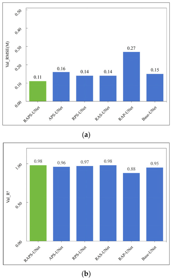
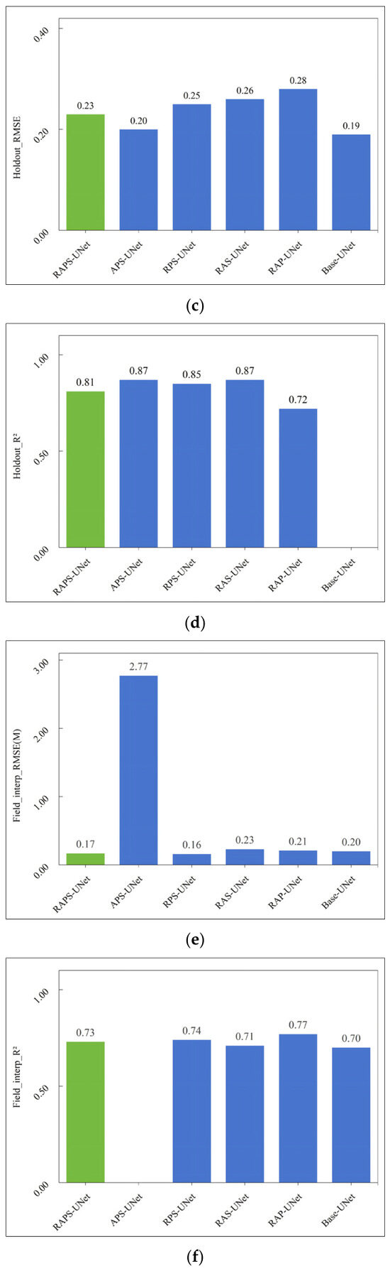
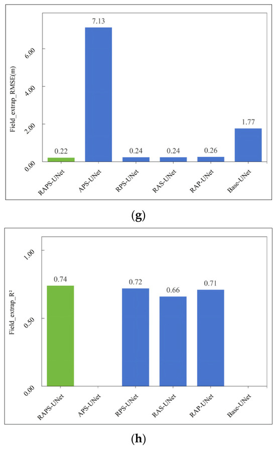
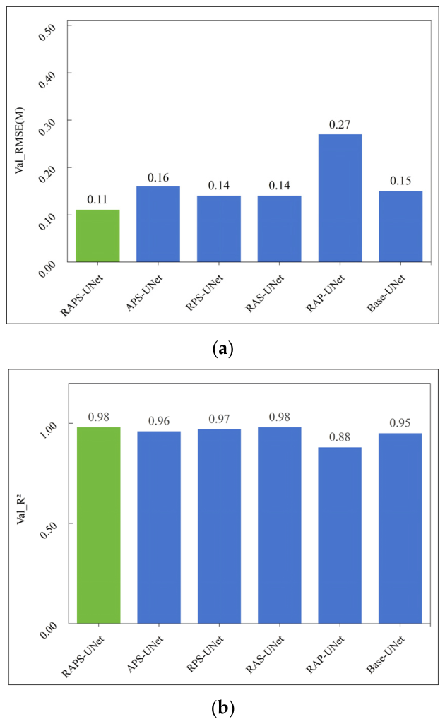
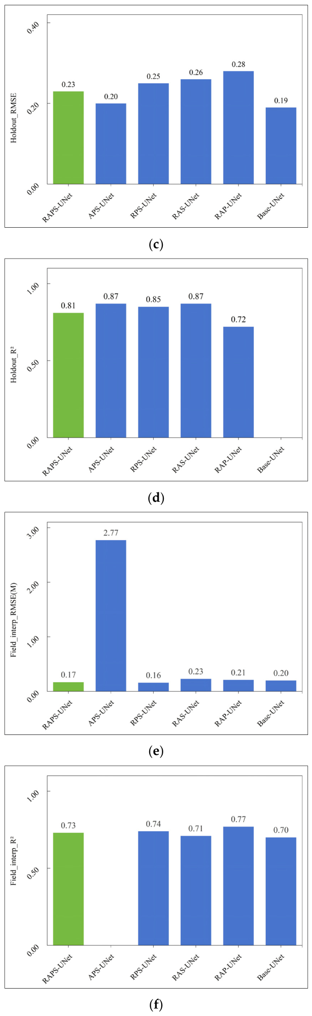
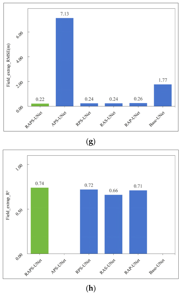
The ablation results are summarized in Table 7, and the corresponding RMSE and R2 comparisons across the four evaluation subsets are visualized in Figure 14a–h. The full RAPS-UNet achieved the best overall performance across all four evaluation subsets, with the lowest Field-extrap RMSE (0.22 m) and consistently strong results on the Val, Holdout, and Field-interp subsets. Variants without residual learning (APS-UNet and Base-UNet) exhibited severe extrapolation degradation despite relatively good validation performance, whereas removing pseudo-label guidance, attention mechanisms, or physics-constrained loss led to smaller but consistent decreases in extrapolation accuracy. These results confirm that all four components contribute to model performance, with residual learning having the largest impact on spatial extrapolation.
Table 7.
Ablation results of RAPS-UNet variants under interpolation and extrapolation-oriented reference sets.
Figure 14.
Summary of ablation experiment results for RAPS-UNet: (a) RMSE comparison on the validation set, (b) R2 comparison on the validation set, (c) RMSE comparison on the Holdout set, (d) R2 comparison on the Holdout set, (e) RMSE comparison on the field_interp set, (f) R2 comparison on the field_interp set, (g) RMSE comparison on the field_extrap set, (h) R2 comparison on the field_extrap set. Caption: The full RAPS-UNet is highlighted for comparison.
5. Discussion
This section discusses the spatial characteristics of inversion uncertainty, the mechanistic contributions of the RAPS-UNet components, the methodological implications of the proposed evaluation protocol, and the limitations and future extensions of this study.
5.1. Spatial Error Characteristics and Extrapolation Uncertainty
The spatial error distribution reveals clear heterogeneity in the inversion uncertainty. Systematic underestimation is mainly observed in the western portion of the study area, which is farthest from the ICESat-2 tracks, whereas slight overestimation occurs closer to the eastern track-covered region. This pattern indicates that prediction uncertainty increases when the model moves away from direct elevation observations. Consistently, the Field-extrap subset shows a higher RMSE than the Field-interp subset, demonstrating the additional uncertainty introduced by spatial extrapolation beyond the effective support of ICESat-2 labels.
Several factors may contribute to this spatially heterogeneous error pattern. In regions without nearby ICESat-2 supervision, the model relies more strongly on the baseline DEM and confidence-weighted pseudo-labels, which may cause the predicted elevation field to approach the large-scale topographic trend rather than fully resolve local variation. Coastal transition zones and permanently inundated water bodies may also introduce mixed-pixel effects and turbidity-related noise, weakening the stability of optical/SAR feature–elevation relationships. In addition, the temporal gap between the remote sensing data used for inversion and the field-surveyed DEM may have contributed to part of the observed discrepancies through actual erosion or deposition during the intervening period.
The relationship between absolute error and distance to the nearest ICESat-2 track further indicates that extrapolation uncertainty does not increase strictly monotonically. Errors are moderate near the tracks, decrease in the intermediate zone, and increase substantially in far-label regions. The near-track errors may be associated with residual photon-height noise, local geolocation uncertainty, and scale mismatch between along-track photon observations and rasterized DEM pixels. In contrast, the error increase in far-label regions reflects the reduced constraint from direct elevation anchors and represents the main extrapolation challenge addressed in this study.
5.2. Mechanistic Contribution of RAPS-UNet Components
The ablation results indicate that residual learning is the primary mechanism supporting stable extrapolation under spatially clustered ICESat-2 label conditions. By predicting residuals relative to a baseline DEM rather than directly estimating absolute elevations, the model operates within a narrower solution space. This residual formulation allows the final prediction to retain the large-scale geomorphic trend provided by the baseline DEM, even in regions where direct elevation labels are sparse or absent. The severe degradation observed in variants without residual learning confirms its central role in full-domain prediction.
The attention mechanisms further improve the selective use of multi-source remote sensing features. In tidal-flat environments, elevation-related signals are mixed with spectral noise, SAR backscatter variability, water–land mixed pixels, and turbidity effects. The CBAMs help emphasize informative optical, SAR, and texture channels, while the Attention Gates reduce the transfer of noise-sensitive encoder features through skip connections. This feature-selection function is particularly useful when heterogeneous remote sensing inputs contribute unevenly to elevation prediction.
The hierarchical pseudo-label strategy extends the effective supervision range beyond the limited ICESat-2 footprint. Instead of assigning equal confidence to all pseudo-labels, RAPS-UNet uses tiered confidence weights according to label provenance and distance from observed regions. This design allows pseudo-labels to provide weak spatial guidance while preventing low-confidence supervision from overwhelming the hard ICESat-2 labels. As a result, pseudo-label augmentation improves full-domain fitting without excessively constraining the model to uncertain auxiliary labels.
Compared with residual learning and pseudo-label guidance, the physics-constrained loss contributes less directly to average accuracy metrics. Its main role is to act as a safeguard against physically implausible predictions in label-sparse regions. Total-variation regularization suppresses unrealistic high-frequency oscillations in the residual field, while the residual-range constraint limits deviations from the baseline DEM within a reasonable range. Therefore, the physics-constrained loss should be interpreted primarily as a stability-enhancing component rather than as the dominant driver of RMSE reduction.
Overall, the performance of RAPS-UNet arises from the complementary roles of its four components. Residual learning provides the main structural prior for extrapolation, attention mechanisms improve multi-source feature fusion, pseudo-label augmentation expands the spatial extent of supervision, and physical constraints reduce unstable residual predictions. Their combination enables more reliable tidal-flat topographic inversion under clustered-label conditions than any single component alone.
5.3. Implications for Small-Scale Tidal-Flat Inversion Under Clustered ICESat-2 Labels
The results highlight the importance of designing evaluation protocols that explicitly account for the spatial structure of ICESat-2 labels. When ICESat-2 observations are spatially clustered, a conventional random validation subset mainly reflects in-distribution fitting performance within the observed label footprint. It cannot adequately assess model behavior in regions without direct elevation supervision, and may therefore overestimate the actual spatial generalization capability of the model.
The four-level evaluation protocol adopted in this study provides a more rigorous assessment framework. The Val subset evaluates model convergence and in-distribution fitting, while the Holdout subset tests label-space extrapolation by excluding a contiguous spatial strip from training, baseline DEM construction, and pseudo-label generation. The Field-interp and Field-extrap subsets further assess real topographic accuracy near and far from ICESat-2 observations using an independent field-surveyed DEM. This design separates interpolation performance from extrapolation performance and provides a clearer basis for evaluating tidal-flat inversion models under clustered-label conditions.
From a methodological perspective, the contribution of RAPS-UNet lies in providing a structured framework for full-domain topographic inversion when high-precision elevation labels are sparse and unevenly distributed. The integration of residual learning, pseudo-label augmentation, attention-based feature fusion, and physics-constrained regularization offers a practical strategy for reducing extrapolation instability in small-scale tidal flats. This framework may also be relevant to other coastal or geomorphological settings where elevation observations are spatially limited, provided that local geomorphic conditions and validation data availability are carefully considered.
5.4. Limitations and Future Work
Although RAPS-UNet alleviates the limitations caused by spatially clustered ICESat-2 labels, systematic errors remain in regions without direct elevation observations. This indicates that extrapolation beyond the effective spatial support of ICESat-2 tracks remains a major source of uncertainty, even when residual learning, pseudo-label augmentation, and physical constraints are incorporated. In addition, the interpolation–extrapolation partition used in this study is based on a distance threshold from ICESat-2 observations; different threshold settings may influence the quantitative characterization of extrapolation uncertainty.
A temporal gap of approximately two years exists between the field-surveyed DEM acquired in November 2024 and the remote sensing data used for inversion from 2019 to 2022. Actual geomorphic changes, including local erosion and deposition, may therefore have contributed to the observed discrepancies. Because contemporaneous validation data were unavailable, the proportion of error attributable to temporal surface change could not be quantitatively isolated in this study.
Another limitation is that the proposed framework was validated within only a single small-scale tidal flat. The objective of this work was to evaluate whether RAPS-UNet can maintain stable full-domain inversion capability under label-clustered ICESat-2 conditions, rather than to demonstrate universal transferability across all coastal environments. Rigorous cross-regional validation remains necessary before the method can be generalized to broader tidal-flat systems. Such validation requires contemporaneous high-precision field-surveyed DEMs across multiple geomorphological and hydrodynamic settings, which remain difficult and costly to acquire because of tidal accessibility constraints and rapid surface changes.
Future work will extend the proposed framework to additional tidal-flat systems with different sedimentary, hydrodynamic, and geomorphic conditions. Cross-regional experiments combined with transfer-learning strategies may help clarify the robustness and transferability of RAPS-UNet. Future studies may also incorporate sediment-dynamics constraints or more advanced semi-supervised paradigms, such as iterative self-training and consistency regularization, to further improve extrapolation stability under extremely sparse-label conditions.
6. Conclusions
This study addressed the limited topographic inversion accuracy caused by the spatially clustered distribution of ICESat-2 laser altimetry data in small-scale tidal flats. A RAPS-UNet framework was proposed by integrating residual learning, attention mechanisms, physics-constrained loss, and semi-supervised pseudo-label augmentation for tidal-flat DEM reconstruction around Dafeng Port, Yancheng. A four-level validation protocol combining random ICESat-2 validation, spatial holdout testing, and field-based interpolation/extrapolation assessment was established to evaluate both in-distribution fitting and spatial extrapolation beyond the ICESat-2 footprint. Validated against the field-surveyed DEM, RAPS-UNet achieved an RMSE of 0.20 m and an R2 of 0.90, reducing the RMSE by approximately 43% relative to the traditional inundation frequency–elevation linear model.
The ablation experiments confirmed the complementary contributions of the four core modules. Residual learning provided the main structural basis for extrapolation beyond the observed label coverage, pseudo-label augmentation extended weak supervision to label-sparse regions, attention mechanisms improved multi-source feature fusion, and the physics-constrained loss helped maintain topographic continuity and physical plausibility. Their integration enabled more stable full-domain inversion under spatially clustered ICESat-2 label conditions.
Overall, this study demonstrates that combining residual learning, pseudo-label augmentation, attention-based feature fusion, and physical constraints can improve tidal-flat topographic inversion under sparse and unevenly distributed elevation labels. The proposed framework provides a practical approach for small-scale tidal-flat DEM reconstruction in analogous data-limited scenarios. Nevertheless, the current validation remains limited to a single study area, and the cross-regional transferability of RAPS-UNet requires further verification using contemporaneous field-surveyed DEMs from additional tidal-flat environments. Future work will explore cross-regional transfer learning and incorporate sediment-dynamics constraints to extend the framework from static single-epoch inversion toward dynamic geomorphic change monitoring.
Author Contributions
Conceptualization, X.L.; Methodology, H.C.; Validation, J.C. (Jiaxin Cui); Formal analysis, H.C., J.C. (Jiaxin Cui) and J.C. (Jiayang Chen); Investigation, Q.L.; Resources, J.C. (Jiayang Chen); Data curation, H.C., J.C. (Jiaxin Cui), J.C. (Jiayang Chen) and Q.L.; Writing—original draft, H.C.; Writing—review & editing, X.L. and F.G.; Supervision, X.L., F.G., J.C. (Jiaxin Cui) and J.C. (Jiayang Chen); Project administration, X.L. and F.G. All authors have read and agreed to the published version of the manuscript.
Funding
This research was funded by the Scientific Research Fund of the Second Institute of Oceanography, Ministry of Natural Resources, grant number JB2602. The APC was jointly funded by the Marine Science and Technology College, Zhejiang Ocean University and the State Key Laboratory of Submarine Geoscience, Second Institute of Oceanography, Ministry of Natural Resources.
Data Availability Statement
The authors would like to thank the National Snow and Ice Data Center (NSIDC) for providing open access to the ICESat-2 ATL03 and ATL08 data products; the State Key Laboratory of Submarine Geoscience, Second Institute of Oceanography, Ministry of Natural Resources, for sharing the in situ measured data used for validation; and the Google Earth Engine (GEE) platform for providing data storage and processing capabilities as well as access to the relevant satellite imagery. Further inquiries can be directed to the corresponding author.
Conflicts of Interest
The authors declare no conflict of interest.
Abbreviations
The following abbreviations are used in this manuscript:
| RMSE | Root Mean Square Error |
| MAE | Mean Absolute Error |
| R2 | Coefficient of Determination |
| DEM | Digital Elevation Model |
| SAR | Synthetic Aperture Radar |
| GEE | Google Earth Engine |
| ICESat-2 | Ice, Cloud, and land Elevation Satellite-2 |
| NSIDC | National Snow and Ice Data Center |
| MNDWI | Modified Normalized Difference Water Index |
| IF | Inundation Frequency |
| NDVI | Normalized Difference Vegetation Index |
| NDWI | Normalized Difference Water Index |
| EVI | Enhanced Vegetation Index |
| AWEI | Automated Water Extraction Index |
| NIR | Near-Infrared |
| SWIR | Shortwave Infrared |
| IVF | Integrated Voting Filter |
| AEF | Adaptive Elliptical Filtering |
| IQR | Interquartile Range |
| DBSCAN | Density-Based Spatial Clustering of Applications with Noise |
| CBAM | Convolutional Block Attention Module |
| AG | Attention Gate |
| GLCM | Gray-Level Co-occurrence Matrix |
| RBF | Radial Basis Function |
| TV | Total Variation |
References
- Lewis, C.J.E.; Carnell, P.E.; Sanderman, J.; Baldock, J.A.; Macreadie, P.I. Variability and Vulnerability of Coastal ‘blue Carbon’ Stocks: A Case Study from Southeast Australia. Ecosystems 2018, 21, 263–279. [Google Scholar]
- Andreu, V.; Gimeno-Garcia, E.; Pascual, J.A.; Vazquez-Roig, P.; Pico, Y. Presence of Pharmaceuticals and Heavy Metals in the Waters of a Mediterranean Coastal Wetland: Potential Interactions and the Influence of the Environment. Sci. Total Environ. 2015, 540, 278–286. [Google Scholar] [PubMed]
- Dyer, K. Muddy Coasts of the World: Processes, Deposits and Function. Estuar. Coast. Shelf Sci. 2003, 57, 1198–1199. [Google Scholar] [CrossRef] [Scilit]
- Zhen, G. Surface Elevation Variation of the Jiangsu Mudflats: Field Observation. Adv. Water Sci. 2014, 25, 880–887. [Google Scholar]
- Gorman, L.; Morang, A.; Larson, R. Monitoring the Coastal Environment; Part Iv: Mapping, Shoreline Changes, and Bathymetric Analysis. J. Coast. Res. 1998, 14, 61–92. [Google Scholar]
- Zhang, X.; Li, H.; Gong, Z.; Zhou, Z.; Dai, W.; Wang, L.; Daramola, S. Method for UAV-based 3D topography reconstruction of tidal creeks. J. Geogr. Sci. 2021, 31, 1852–1872. [Google Scholar] [CrossRef] [Scilit]
- Zeng, W. Fusing Optical and SAR Remote Sensing Data for Extracting Costal Wetlands Information in Guangdong-Hong Kong-Macao Great Bay Area. Master’s Thesis, Guangzhou University, Guangzhou, China, 2022. (In Chinese) [Google Scholar]
- Li, J.; Zhang, B.; Zhang, L.; Wang, Z.; Song, K. Current Status and Prospect of Researches on Wetland Monitoring Based on Remote Sensing. Prog. Geogr. 2007, 26, 33–43. (In Chinese) [Google Scholar]
- Sun, S.; Zhang, Y.; Song, Z.; Chen, B.; Zhang, Y.; Yuan, W.; Chen, C.; Chen, W.; Ran, X.; Wang, Y. Mapping Coastal Wetlands of the Bohai Rim at a Spatial Resolution of 10 M Using Multiple Open-Access Satellite Data and Terrain Indices. Remote Sens. 2020, 12, 4114. [Google Scholar] [CrossRef] [Scilit]
- Shapiro, A.C.; Trettin, C.C.; Kuechly, H.; Alavinapanah, S.; Bandeira, S. The Mangroves of the Zambezi Delta: Increase in Extent Observed via Satellite from 1994 to 2013. Remote Sens. 2015, 7, 16504–16518. [Google Scholar] [CrossRef] [Scilit]
- Ning, X.; Chang, W.; Wang, H.; Zhang, H.; Zhu, Q. Extraction of marsh wetland in Heilongjiang Basin based on GEE and multi-source remote sensing data. Natl. Remote Sens. Bull. 2022, 26, 386–396. (In Chinese) [Google Scholar] [CrossRef] [Scilit]
- Wang, J.; Huang, H.; Jia, H.; Zheng, S.; Zhao, M.; Chen, M.; Zhang, X.; Zhuang, D. Discussion on the strategies of coastal ecosystem protection and restoration in the Guangdong-Hong Kong-Macao Greater Bay Area. Acta Ecol. Sin. 2020, 40, 8430–8439. (In Chinese) [Google Scholar] [CrossRef] [Scilit]
- Mason, D.C.; Davenport, I.J.; Robinson, G.; Flather, R.A.; Mccartney, B.S. Construction of an Inter-tidal Digital Elevation Model by the ‘water-line’ Method. Geophys. Res. Lett. 1995, 22, 3187–3190. [Google Scholar] [CrossRef] [Scilit]
- Tseng, K.; Kuo, C.; Lin, T.; Huang, Z.; Lin, Y.; Liao, W.; Chen, C. Reconstruction of time-varying tidal flat topography using optical remote sensing imageries. ISPRS-J. Photogramm. Remote Sens. 2017, 131, 92–103. [Google Scholar] [CrossRef] [Scilit]
- Wu, Z.; Zhao, Y.; Wu, S.; Chen, H.; Song, C.; Mao, Z.; Shen, W. Satellite-Derived Bathymetry Using a Fast Feature Cascade Learning Model in Turbid Coastal Waters. J. Remote Sens. 2024, 4, 0272. [Google Scholar] [CrossRef] [Scilit]
- Zhang, S.; Xu, Q.; Wang, H.; Kang, Y.; Li, X. Automatic Waterline Extraction and Topographic Mapping of Tidal Flats from SAR Images Based on Deep Learning. Geophys. Res. Lett. 2022, 49, e2021GL096007. [Google Scholar] [CrossRef] [Scilit]
- Qian, S.; Chen, Y.; Wang, W.; Zhang, G.; Li, L.; Hao, Z.; Wang, Y. Physics-guided Deep Neural Networks for Bathymetric Mapping Using Sentinel-2 Multi-Spectral Imagery. Front. Mar. Sci. 2025, 12, 1636124. [Google Scholar] [CrossRef] [Scilit]
- Dubayah, R.; Blair, J.B.; Goetz, S.; Fatoyinbo, L.; Hansen, M.; Healey, S.; Hofton, M.; Hurtt, G.; Kellner, J.; Luthcke, S.; et al. The Global Ecosystem Dynamics Investigation: High-resolution Laser Ranging of the Earth’s Forests and Topography. Sci. Remote Sens. 2020, 1, 100002. [Google Scholar] [CrossRef] [Scilit]
- Parrish, C.E.; Magruder, L.A.; Neuenschwander, A.L.; Forfinski-Sarkozi, N.; Alonzo, M.; Jasinski, M. Validation of ICESat-2 ATLAS Bathymetry and Analysis of ATLAS’s Bathymetric Mapping Performance. Remote Sens. 2019, 11, 1634. [Google Scholar] [CrossRef] [Scilit]
- Albright, A.; Glennie, C. Nearshore Bathymetry from Fusion of Sentinel-2 and ICESat-2 Observations. IEEE Geosci. Remote Sens. Lett. 2021, 18, 900–904. [Google Scholar] [CrossRef] [Scilit]
- Thomas, N.; Pertiwi, A.P.; Traganos, D.; Lagomasino, D.; Poursanidis, D.; Moreno, S.; Fatoyinbo, L. Space-Borne Cloud-Native Satellite-Derived Bathymetry (SDB) Models Using Icesat-2 and Sentinel-2. Geophys. Res. Lett. 2021, 48, e2020GL092170. [Google Scholar] [CrossRef] [Scilit]
- Xu, N.; Ma, Y.; Yang, J.; Wang, X.H.; Wang, Y.; Xu, R. Deriving Tidal Flat Topography Using ICESat-2 Laser Altimetry and Sentinel-2 Imagery. Geophys. Res. Lett. 2022, 49, e2021GL096813. [Google Scholar] [CrossRef] [Scilit]
- Zheng, X.; Zhou, B.; Lei, H.; Jin, Y.; Su, Q. Mapping Tidal Flat Topography Using Time-Series Sentinel-2 Images and ICESat-2 Data: A Case Study in Cixi City. Ocean Coast. Manag. 2024, 256, 107278. [Google Scholar] [CrossRef] [Scilit]
- Tang, P.; Guo, S.; Qie, L.; Zhang, X.; Fang, H.; Wan, L.; Chanussot, J.; Du, P. Tidal flat topography mapping with Sentinel time series using cross-modal sample transfer and deep learning. ISPRS-J. Photogramm. Remote Sens. 2025, 225, 69–87. [Google Scholar] [CrossRef] [Scilit]
- Xin, H.; Xu, N.; Xu, H.; Yang, H.; Wang, Z.; Zhang, Z.; Ding, Y.; Luan, H.; Ou, Y.; Yang, Y. Mapping Tidal Flat Topography by Combining ICESat-2 Laser Altimetry and Multi-Source Satellite Imagery. Int. J. Digit. Earth 2025, 18, 2554313. [Google Scholar] [CrossRef] [Scilit]
- Lee, D. Pseudo-Label: The Simple and Efficient Semi-Supervised Learning Method for Deep Neural Networks. In Proceedings of the ICML 2013 Workshop: Challenges in Representation Learning (WREPL), Atlanta, GA, USA, 21 June 2013. [Google Scholar]
- Tarvainen, A.; Valpola, H. Mean Teachers Are Better Role Models: Weight-averaged Consistency Targets Improve Semi-Supervised Deep Learning Results. Adv. Neural Inf. Process. Syst. 2017, 30, 1195–1204. [Google Scholar] [CrossRef]
- Sohn, K.; Berthelot, D.; Li, C.; Zhang, Z.; Carlini, N.; Cubuk, E.D.; Kurakin, A.; Zhang, H.; Raffel, C. FixMatch: Simplifying Semi-Supervised Learning with Consistency and Confidence. Adv. Neural Inf. Process. Syst. 2020, 33, 596–608. [Google Scholar]
- Wang, Y.; Albrecht, C.M.; Braham, N.A.A.; Mou, L.; Zhu, X.X. Self-supervised Learning in Remote Sensing: A Review. IEEE Geosci. Remote Sens. Mag. 2022, 10, 213–247. [Google Scholar] [CrossRef] [Scilit]
- Zhou, Z. A Brief Introduction to Weakly Supervised Learning. Natl. Sci. Rev. 2018, 5, 44–53. [Google Scholar]
- Raissi, M.; Perdikaris, P.; Karniadakis, G.E. Physics-informed Neural Networks: A Deep Learning Framework for Solving Forward and Inverse Problems Involving Nonlinear Partial Differential Equations. J. Comput. Phys. 2019, 378, 686–707. [Google Scholar] [CrossRef] [Scilit]
- Karniadakis, G.E.; Kevrekidis, I.G.; Lu, L.; Perdikaris, P.; Wang, S.; Yang, L. Physics-informed Machine Learning. Nat. Rev. Phys. 2021, 3, 422–440. [Google Scholar] [CrossRef] [Scilit]
- Willard, J.; Jia, X.; Xu, S.; Steinbach, M.; Kumar, V. Integrating Scientific Knowledge with Machine Learning for Engineering and Environmental Systems. ACM Comput. Surv. 2023, 55, 1–37. [Google Scholar] [CrossRef] [Scilit]
- Daw, A.; Karpatne, A.; Watkins, W.; Read, J.; Kumar, V. Physics-Guided Neural Networks (PGNN): An Application in Lake Temperature Modeling; Chapman and Hall/CRC: Boca Raton, FL, USA, 2017. [Google Scholar]
- Reichstein, M.; Camps-Valls, G.; Stevens, B.; Jung, M.; Denzler, J.; Carvalhais, N.; Prabhat. Deep Learning and Process Understanding for Data-Driven Earth System Science. Nature 2019, 566, 195–204. [Google Scholar] [CrossRef] [Scilit] [PubMed]
- He, J.; Fu, C.; Shu, L.; Zhang, G.; Wan, K. Analysis on the status quo and causes of erosion and deposition of Yancheng coastline in Jiangsu Province. J. Geol. 2021, 45, 189–196. (In Chinese) [Google Scholar]
- Neumann, T.A.; Hancock, D.; Robbins, J.; Gibbons, A.; Lee, J.; Brenner, A.; Felikson, D.; Harbeck, K.; Saba, J.; Luthcke, S.; et al. Ice, Cloud, and Land Elevation Satellite (ICESat-2) Project Algorithm Theoretical Basis Document (ATBD) for Global Geolocated Photons ATL03, Version 7. ICESat-2 Project, 2025. Available online: https://nsidc.org/sites/default/files/documents/technical-reference/icesat2_atl03_atbd_v007.pdf (accessed on 5 June 2026).
- Neuenschwander, A.; Pitts, K.; Jelley, B.; Robbins, J.; Markel, J.; Popescu, S.; Nelson, R.; Harding, D.; Pederson, D.; Klotz, B.; et al. Ice, Cloud, and Land Elevation Satellite (ICESat-2) Project Algorithm Theoretical Basis Document (ATBD) for Land-Vegetation Along-Track Products (ATL08), Version 7. ICESat-2 Project, 2024. Available online: https://nsidc.org/sites/default/files/documents/technical-reference/icesat2_atl08_atbd_v007.pdf (accessed on 5 June 2026).
- Xu, H. Modification of Normalised Difference Water Index (NDWI) to Enhance Open Water Features in Remotely Sensed Imagery. Int. J. Remote Sens. 2006, 27, 3025–3033. [Google Scholar] [CrossRef] [Scilit]
- Sun, F.; Sun, W.; Chen, J.; Gong, P. Comparison and improvement of methods for identifying waterbodies in remotely sensed imagery. Int. J. Remote Sens. 2012, 33, 6854–6875. [Google Scholar] [CrossRef] [Scilit]
- Ma, S.; Wang, N.; Zhou, L.; Yu, J.; Chen, X.; Chen, Y. Inversion of Tidal Flat Topography Based on the Optimised Inundation Frequency Method—A Case Study of Intertidal Zone in Haizhou Bay, China. Remote Sens. 2024, 16, 685. [Google Scholar] [CrossRef] [Scilit]
- Mukherjee, A. Effect of Urbanisation & Population Density on Groundwater in India Using Satellite Remote Sensing Data. Doctoral Dissertation, Indian Institute of Science, Bangalore, India, 2021. [Google Scholar]
- Aliihsan, S. A Survey on Global Thresholding Methods for Mapping Open Water Body Using Sentinel-2 Satellite Imagery and Normalized Difference Water Index. Arch. Comput. Methods Eng. 2020, 28, 1335–1347. [Google Scholar] [CrossRef] [Scilit]
- Drusch, M.; Del Bello, U.; Carlier, S.; Colin, O.; Fernandez, V.; Gascon, F.; Hoersch, B.; Isola, C.; Laberinti, P.; Martimort, P.; et al. Sentinel-2: ESA’s Optical High-Resolution Mission for GMES Operational Services. Remote Sens. Environ. 2012, 120, 25–36. [Google Scholar] [CrossRef] [Scilit]
- McFeeters, S.K. The Use of the Normalized Difference Water Index (ndwi) in the Delineation of Open Water Features. Int. J. Remote Sens. 1996, 17, 1425–1432. [Google Scholar] [CrossRef] [Scilit]
- Tucker, C.J. Red and Photographic Infrared Linear Combinations for Monitoring Vegetation. Remote Sens. Environ. 1979, 8, 127–150. [Google Scholar] [CrossRef] [Scilit]
- Huete, A.; Didan, K.; Miura, T.; Rodriguez, E.P.; Gao, X.; Ferreira, L.G. Overview of the Radiometric and Biophysical Performance of the MODIS Vegetation Indices. Remote Sens. Environ. 2002, 83, 195–213. [Google Scholar] [CrossRef] [Scilit]
- Feyisa, G.L.; Meilby, H.; Fensholt, R.; Proud, S.R. Automated Water Extraction Index: A New Technique for Surface Water Mapping Using Landsat Imagery. Remote Sens. Environ. 2014, 140, 23–35. [Google Scholar] [CrossRef] [Scilit]
- Sagar, S.; Roberts, D.; Bala, B.; Lymburner, L. Extracting the Intertidal Extent and Topography of the Australian Coastline from a 28 Year Time Series of Landsat Observations. Remote Sens. Environ. 2017, 195, 153–169. [Google Scholar] [CrossRef] [Scilit]
- Murray, N.J.; Phinn, S.R.; DeWitt, M.; Ferrari, R.; Johnston, R.; Lyons, M.B.; Clinton, N.; Thau, D.; Fuller, R.A. The Global Distribution and Trajectory of Tidal Flats. Nature 2018, 565, 222–225. [Google Scholar] [CrossRef] [Scilit] [PubMed]
- Torres, R.; Snoeij, P.; Geudtner, D.; Bibby, D.; Davidson, M.; Attema, E.; Potin, P.; Rommen, B.; Floury, N.; Brown, M.; et al. GMES Sentinel-1 Mission. Remote Sens. Environ. 2012, 120, 9–24. [Google Scholar] [CrossRef] [Scilit]
- Tsyganskaya, V.; Martinis, S.; Marzahn, P.; Ludwig, R. SAR-based Detection of Flooded Vegetation—A Review of Characteristics and Approaches. Int. J. Remote Sens. 2018, 39, 2255–2293. [Google Scholar] [CrossRef] [Scilit]
- Mahdianpari, M.; Salehi, B.; Mohammadimanesh, F.; Brisco, B.; Homayouni, S.; Gill, E.; DeLancey, E.R.; Bourgeau-Chavez, L. The First Wetland Inventory Map of Newfoundland at a Spatial Resolution of 10 M Using Sentinel-1 and Sentinel-2 Data on the Google Earth Engine Cloud Computing Platform. Can. J. Remote Sens. 2020, 11, 43. [Google Scholar]
- Haralick, R.M.; Shanmugam, K.; Dinstein, I.H. Textural Features for Image Classification. IEEE Trans. Syst. Man Cybern. 1973, SMC-3, 610–621. [Google Scholar] [CrossRef] [Scilit]
- Yu, A.; Quan, Y.; Yu, R.; Guo, W.; Wang, X.; Hong, D.; Zhang, H.; Chen, J.; Hu, Q.; He, P. Deep Learning Methods for Semantic Segmentation in Remote Sensing with Small Data: A Survey. Remote Sens. 2023, 15, 4987. [Google Scholar] [CrossRef] [Scilit]
- Yue, L.; Shen, H.; Zhang, L.; Zheng, X.; Zhang, F.; Yuan, Q. High-Quality Seamless Dem Generation Blending Srtm-1, Aster Gdem V2 and Icesat/Glas Observations. ISPRS-J. Photogramm. Remote Sens. 2017, 123, 20–34. [Google Scholar] [CrossRef] [Scilit]
- He, K.; Zhang, X.; Ren, S.; Sun, J. Deep Residual Learning for Image Recognition. In Proceedings of the 2016 IEEE Conference on Computer Vision and Pattern Recognition (CVPR), Las Vegas, NV, USA, 27–30 June 2016. [Google Scholar]
- Woo, S.; Park, J.; Lee, J.; Kweon, I.S. CBAM: Convolutional Block Attention Module. In Proceedings of the European Conference on Computer Vision (ECCV), Munich, Germany, 8–14 September 2018; pp. 3–19. [Google Scholar]
- Oktay, O.; Schlemper, J.; Le Folgoc, L.; Lee, M.; Heinrich, M.; Misawa, K.; Mori, K.; McDonagh, S.; Hammerla, N.Y.; Kainz, B.; et al. Attention U-Net: Learning Where to Look for the Pancreas. In Proceedings of the Medical Imaging with Deep Learning (MIDL), Amsterdam, The Netherlands, 4–6 July 2018. [Google Scholar]

Disclaimer/Publisher’s Note: The statements, opinions and data contained in all publications are solely those of the individual author(s) and contributor(s) and not of MDPI and/or the editor(s). MDPI and/or the editor(s) disclaim responsibility for any injury to people or property resulting from any ideas, methods, instructions or products referred to in the content. |
© 2026 by the authors. Licensee MDPI, Basel, Switzerland. This article is an open access article distributed under the terms and conditions of the Creative Commons Attribution (CC BY) license.