


Highlights
What are the main findings?
- A novel intensity–trend–stability framework reveals dynamic trade-offs and synergies among ecosystem services under future land-use scenarios.
- Stable trade-offs between water yield and other services coexist with robust synergies among soil retention, carbon sequestration, and habitat quality, with clear scale effects.
What are the implications of the main findings?
- The framework enables spatial identification of conflict zones, synergistic hotspots, and transition areas for ecological zoning.
- Results provide a transferable approach for scenario-based land-use planning and adaptive ecosystem management.
Abstract
Dynamic trade-offs and synergies among ecosystem services (ESs) are highly sensitive to land-use change, spatial scale, and future uncertainty. However, most ES-based zoning studies rely on static assessments that overlook temporal dynamics and scenario robustness. To address this limitation, we propose a novel intensity–trend–stability framework that integrates historical interaction strength, projected future trajectories, and cross-scenario consistency to assess and spatially zone ES interactions. The framework was applied to the Songnen Plain, China, using multi-scale analysis and four contrasting land-use scenarios for 2030. An XGBoost–SHAP model was further employed to identify key drivers and nonlinear effects underlying ES interaction dynamics. Results show that (1) land-use transitions exhibit strong scenario dependency under different development pathways. (2) Water yield consistently exhibits trade-offs with other ESs, whereas soil retention, carbon sequestration, and habitat quality maintain stable synergies, with interaction intensity generally weakening at coarser scales. (3) The proposed framework effectively identifies stable conflict zones, synergistic hotspots, and transitional areas, with HHH zones of water-related interactions accounting for 30.72–37.43% of the study area, while LLH zones of other ES pairs each occupy more than 39%. (4) Climatic and topographic factors primarily regulate water-related interactions, whereas vegetation conditions and landscape configuration dominate synergistic ES relationships, with pronounced nonlinear threshold effects. The proposed framework improves the detection of dynamic ES interaction patterns and supports scenario-based ecological zoning and sustainable land-use management.
1. Introduction
Ecosystem services (ESs) represent the diverse benefits that humans obtain directly or indirectly from ecosystems [1]. The sustained provision of multiple ESs underpins human well-being, economic development, and societal sustainability [2,3]. However, accelerating global environmental change is affecting ecosystem functions and service provision, resulting in pronounced spatial and temporal heterogeneity [4]. In response, ES-based ecological zoning has emerged as an important approach for supporting spatial planning and ecosystem management by delineating management units according to dominant service functions and interaction characteristics [5]. By aligning conservation priorities with ecosystem service dynamics, such zoning strategies provide an effective means of balancing ecological protection and socio-economic development.
Interactions among ESs are commonly characterized as synergies and trade-offs [6], reflecting situations in which multiple services increase simultaneously or where gains in one service occur at the expense of another [7]. Understanding these interaction patterns has become a central focus of ES research because they provide the conceptual basis for identifying ES bundles and designing differentiated management strategies. Consequently, many ecological zoning frameworks have been developed to identify areas dominated by strong synergies or severe trade-offs, thereby supporting targeted conservation or restoration actions [8]. However, most existing approaches remain inherently static, as they are typically based on ES bundles or interaction patterns derived from a single time period [9]. For instance, Huang et al. [7] conducted ecological zoning in the Tana River Basin, Kenya, based on pairwise ES interactions, but their analysis was restricted to a single year and therefore overlooked the temporal evolution of ES relationships. Similarly, Yin et al. [4] grouped sub-watersheds in China’s Yellow River Basin, centering on three Water-Energy-Food nexus-related ESs, but their zoning excluded prospective shifts in ES interactions under alternative future development scenarios. Such static assessments fail to capture the dynamic changes in ES relationships, as synergies and trade-offs may reverse under external disturbances. As a result, zoning decisions based solely on historical or current ES states lack foresight and are insufficient for long-term ecological management.
To address this limitation, scenario-based simulations integrating ES models (e.g., InVEST [10], RUSLE [9], EROSION 3D [11]) with land-use change models (e.g., PLUS [12], FLUS [13]) have increasingly been used to explore potential ES interactions under alternative development pathways. These approaches provide valuable insights into future dynamics and have begun to support forward-looking zoning [14]. Nevertheless, a critical limitation remains: the robustness of zoning outcomes across alternative scenarios is insufficiently evaluated. Given the inherent uncertainty of future social-ecological evolution, zoning formulated based on a single scenario tends to be one-sided and ignores diverse development possibilities. Without explicitly considering cross-scenario consistency, current approaches lack a systematic mechanism to assess the stability and reliability of ES interaction patterns, which limits their practical applicability for decision-making.
In addition to temporal and scenario uncertainties, spatial scale represents another critical challenge in ES interaction assessments [8]. Ecological processes, landscape structures, and human disturbances operate across multiple spatial scales, often causing the strength and direction of ES interactions to vary with analytical resolution [15,16]. For instance, synergies detected at coarse scales may mask fine-scale trade-offs, while grid-based analyses may not correspond to actual management or planning units [17]. Despite the well-recognized scale sensitivity, most ES-based zoning studies adopt a single predetermined spatial scale for practical constraints [7]. Such practices may create mismatches between ecological processes and management units, potentially biasing zoning outcomes and weakening their policy relevance [4]. Therefore, systematic multi-scale comparisons are essential for identifying spatial units that best capture ES interaction dynamics while supporting practical ecosystem management and ecological zoning.
Beyond identifying interaction patterns, understanding their underlying drivers is equally crucial for effective ecosystem management. ES interactions are shaped by a complex interplay of climatic conditions, landscape configuration, and human activities, often exhibiting nonlinear responses and threshold effects [9]. Conventional statistical approaches, such as correlation analysis [18], linear regression [19], and geographical detector model [20], have been widely used to identify ES drivers but often struggle to capture complex nonlinear relationships. In contrast, interpretable machine-learning approaches integrating eXtreme Gradient Boosting (XGBoost 2.1.2) with SHapley Additive exPlanations (SHAP) provide a powerful framework for identifying dominant drivers, quantifying nonlinear effects, and detecting critical thresholds [21]. Despite these advantages, such approaches remain rarely applied in ES interaction research, particularly in the context of ecological zoning.
Taken together, current ES-based zoning approaches face several limitations, including static assessments of ES interactions, insufficient evaluation of cross-scenario robustness, limited consideration of scale effects, and inadequate understanding of underlying drivers. Addressing these gaps requires an integrated framework capable of simultaneously capturing the intensity, temporal trajectory, and stability of ES interactions across multiple scenarios and spatial scales.
To this end, we propose a novel three-dimensional “intensity–trend–stability” framework for dynamic zoning of ES interactions. The Songnen Plain in China is selected as the study area. The PLUS-based land-use simulations, InVEST modeling, multi-scale analysis, and XGBoost–SHAP interpretation are jointly applied. This study intends to: (1) simulate land-use transitions from 2020 to 2030 and assess associated ES interaction dynamics; (2) examine scale dependence and identify the most suitable spatial resolution for robust ecological zoning; and (3) identify dominant drivers and critical thresholds governing the emergence and transformation of ES interactions. By linking historical dynamics, future trajectories, and cross-scenario stability, this study provides a forward-looking and interpretable framework for identifying ES interaction and translating them into policy-relevant ecological zoning strategies, offering transferable insights for sustainable land-use planning and adaptive ecosystem governance.
2. Materials and Methods
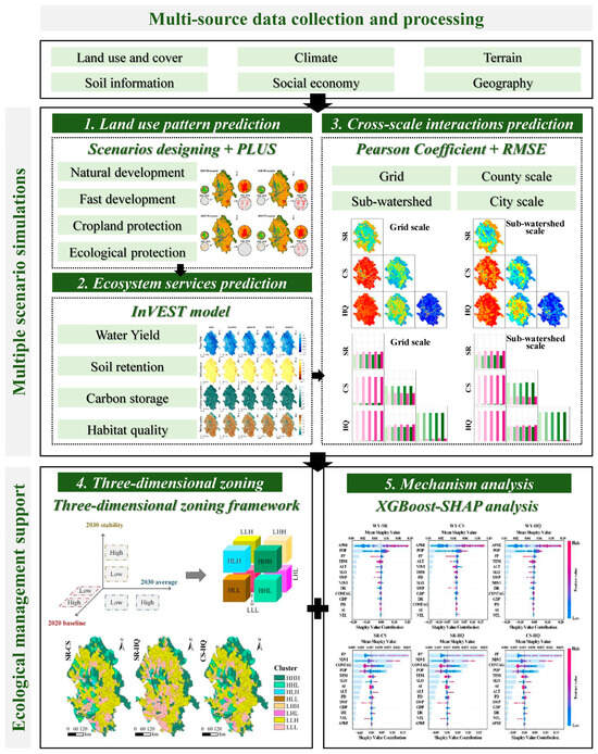
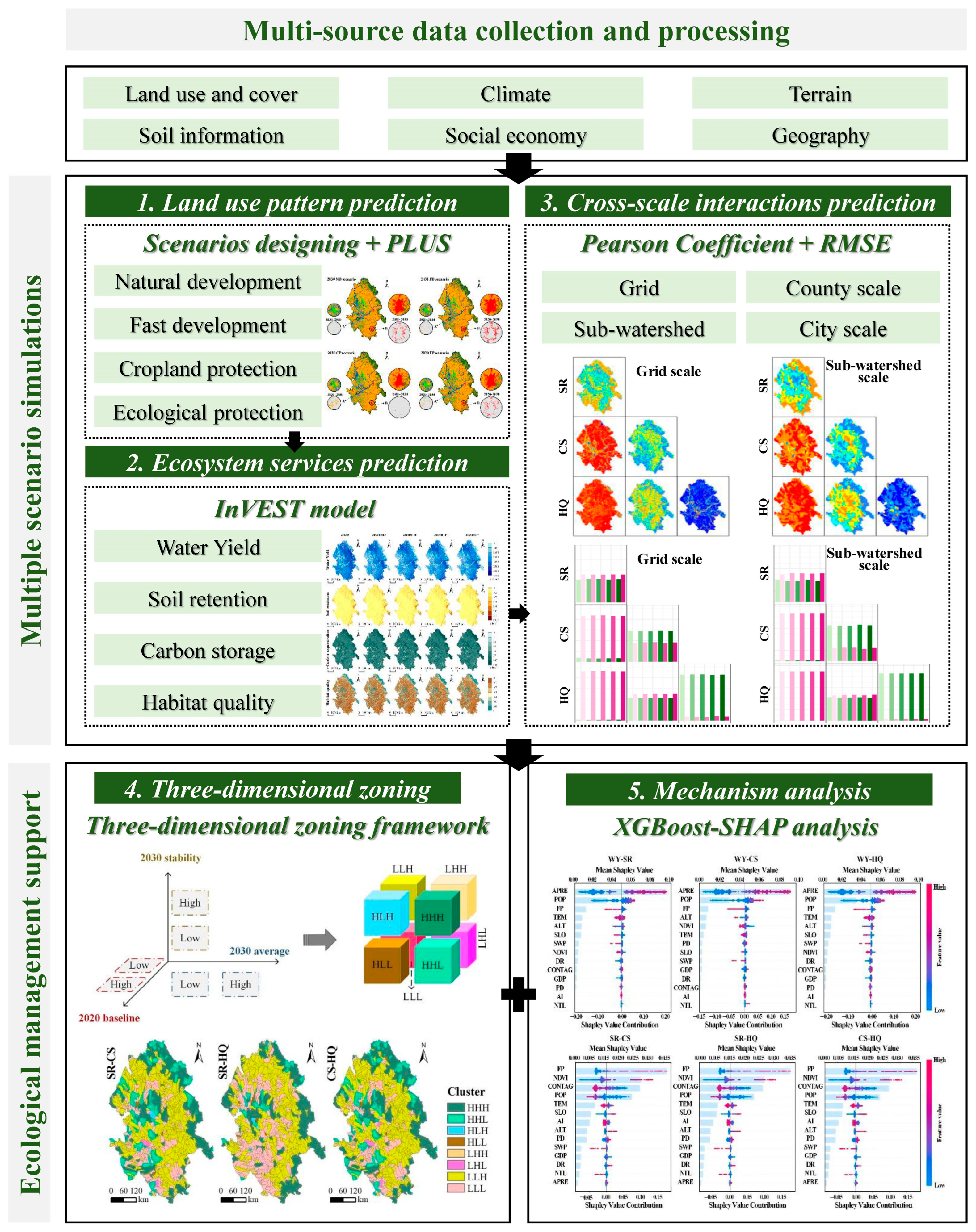
The research was conducted through five sequential steps. First, we pre-processed the multi-source datasets used in this study. Second, we designed multiple 2030 land-use scenarios and simulated their potential spatial configurations. Third, we quantified the multi-scale interactions among four key ESs for 2020 and across the 2030 scenarios. Fourth, we delineated the ecological zones by applying the proposed three-dimensional zoning framework. Finally, we analyzed the effects of natural factors and anthropogenic disturbances on ES interactions, identifying both the key drivers and nonlinear effects for ES sustainability. A detailed framework and applied methods are shown in Figure 1. This study adopts the approaches for conducting the third step from our previous work, which mainly examined the scale dependence of ES during historical periods [8]. However, unlike the prior study, this research focused on the potential evolution of ES interaction under future scenarios and aimed to fill the research gaps outlined in the Introduction.
Figure 1.
Framework of the research.
2.1. Study Area
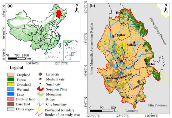
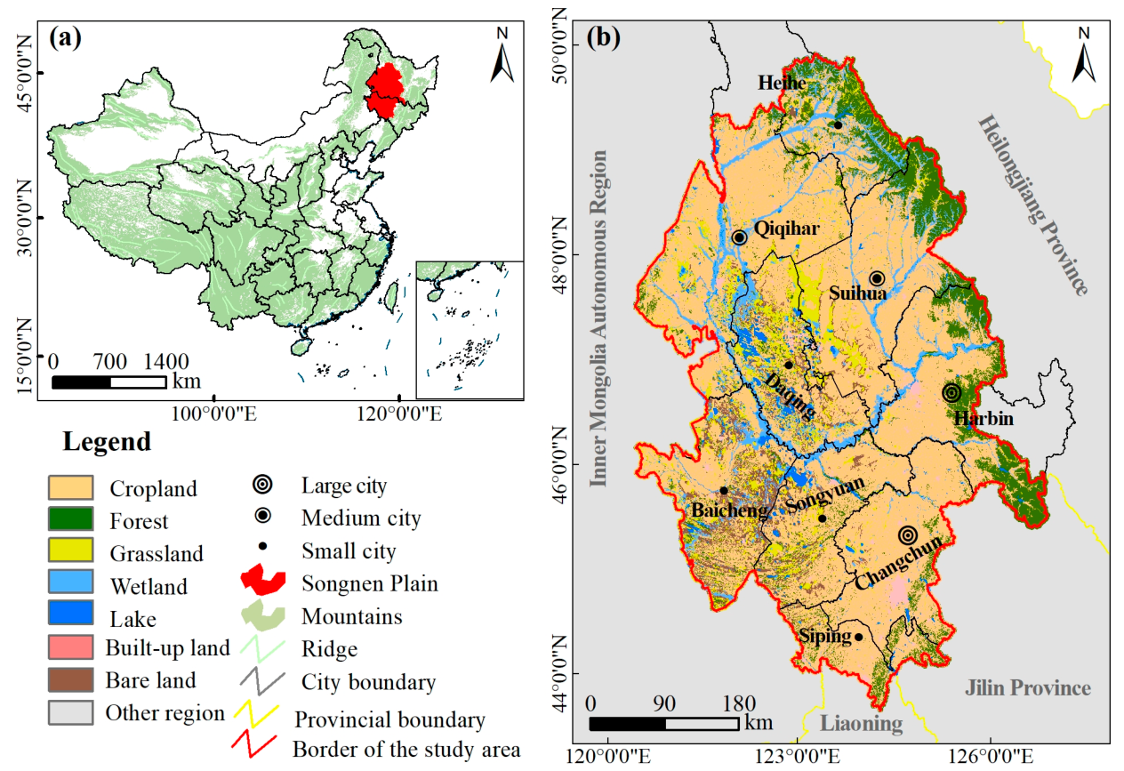
The Songnen Plain is situated in Northeast China, geographically distributed between 121°38′~128°33′E longitude and 42°49′~49°12′N latitude [21]. Topographically, the plain is predominantly characterized by flat terrain, being geomorphologically bounded by the Greater Khingan Range to the west, the Lesser Khingan Range to the north, and the Changbai Mountains to the east (Figure 2). Elevation varies between 92 and 1696 m, with the majority of the region lying under 200 m. Its precipitation [22] and temperature [23] decrease from east to west.
Figure 2.
Map of the Songnen Plain: (a) location and (b) land types.
As one of China’s most important grain-producing regions and a representative agriculture–wetland composite ecosystem, the region is characterized by intensive agricultural production, widespread wetlands, and rapidly evolving land-use policies [8]. In recent decades, large-scale wetland restoration, cropland protection, and ecological conservation initiatives have fundamentally reshaped land-use patterns, creating pronounced spatial heterogeneity and policy-driven uncertainty in ecosystem service provision [21]. Meanwhile, the coexistence of agricultural expansion, soil erosion risks in black soil areas, and water regulation pressures generates complex trade-offs among provisioning and regulating services [24]. These characteristics make the Songnen Plain a typical and policy-sensitive plain region where ES interactions are highly dynamic across space, time, and scales, providing an ideal testing ground for developing a robust, scenario-oriented zoning framework.
2.2. Data Source and Preprocessing
This study adopts multiple remote sensing datasets, including the land use/cover changes database of China (CNLUCC), monthly climate datasets, the NASADEM V001 product [25], the Normalized Difference Vegetation Index (NDVI) product, and the annual nighttime light (NTL) product [26], among others. Detailed information and its applications in model calculations are summarized in Table 1. The CNLUCC during 2010–2020 provided by the Chinese Academy of Sciences, was applied to analyze the dynamics of land types, which were reclassified into cropland, forest, grassland, wetland, water area, built-up land, and bare land for future scenario prediction and ES assessment. The MODIS NDVI product was obtained from the National Aeronautics and Space Administration (https://www.nasa.gov/, accessed on 11 December 2025). The monthly climate datasets, containing precipitation, temperature, and evapotranspiration, were obtained from the National Earth System Science Data Center (https://www.geodata.cn/, accessed on 11 December 2025). The NASADEM V001 product was selected to obtain terrain information by calculating altitude and slope. The geography datasets acquired from the National Catalogue Service for Geographic Information (https://www.webmap.cn, accessed on 11 December 2025) were used to measure residential density and distances to roads, railways, and rivers. Soil information was obtained from the World Soil Information (https://www.isric.org/, accessed on 12 October 2024) and the depth to bedrock map [27]. Annual population density from the WorldPop Platform (https://hub.worldpop.org/, accessed on 11 December 2025) and the annual nighttime light product [26] were applied to indicate social economy development. The vector file of sub-watersheds was obtained from the public HydroBasins database (https://www.hydrosheds.org/, accessed on 02 September 2025). In order to meet the requirements of PLUS and InVEST models, all these datasets were projected into the Asia North Albers Equal Area Conic coordinate system and resampled at a 100 m spatial resolution. For all InVEST simulations across the four 2030 scenarios, we adopted static 2020 baseline climate data, including precipitation, mean temperature, and evapotranspiration. This is a deliberate research design: our study focuses specifically on the ecological impacts caused by future land-use transitions and differentiated land management policies. By keeping climate conditions unchanged, we can effectively isolate the contribution of land cover change to ecosystem services. For further optimization of the analytical framework in future research, higher-resolution remote sensing products are recommended, such as land cover maps derived from Sentinel-2 imagery.
Table 1.
Description of datasets employed in this study.
2.3. Multi-Scenario Prediction for Future Land Allocation
2.3.1. Scenario Designing
To explore the potential impacts of alternative development pathways on ES interactions, four land-use scenarios were constructed, including natural development (ND), fast development (FD), cropland protection (CP), and ecological protection (EP). These scenarios represent contrasting socio-economic and policy orientations commonly adopted in land system studies.
The ND scenario assumes a continuation of historical land-use transition trajectories observed during 2010–2020, serving as a business-as-usual baseline without additional policy intervention. Based on this baseline, three policy-oriented scenarios were developed by systematically modifying transition probabilities for specific land-use categories. Specifically, in the FD scenario, the transition probability toward built-up land was increased to simulate accelerated urban expansion. In the CP scenario, the conversion of cropland to other land types was restricted to reflect farmland protection policies. In the EP scenario, the expansion probabilities of ecological land types (i.e., forest, grassland, wetland, and water bodies) were increased while limiting their conversion to other uses, representing ecological conservation priorities.
We set a unified ±15% adjustment range to calibrate land-use transition probabilities across all policy scenarios. The core underlying assumption is that moderate and identical numerical perturbations can effectively distinguish divergent development orientations and avoid extreme and unrealistic land conversion trends. This moderate adjustment relative to historical transition rules is not formulated to fit actual local policy implementation targets but to build a unified quasi-experimental comparison framework. This treatment guarantees consistent experimental conditions among scenarios and enables us to quantitatively reveal the response differences in ES interactions under varied development preferences. Such a design ensures comparability across scenarios and enables a systematic evaluation of how different development priorities influence ES interactions under consistent experimental conditions. In this sense, the scenario setting can be regarded as a quasi-experimental framework that isolates policy-driven land-use effects while maintaining internal consistency.
2.3.2. PLUS Model
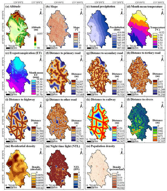
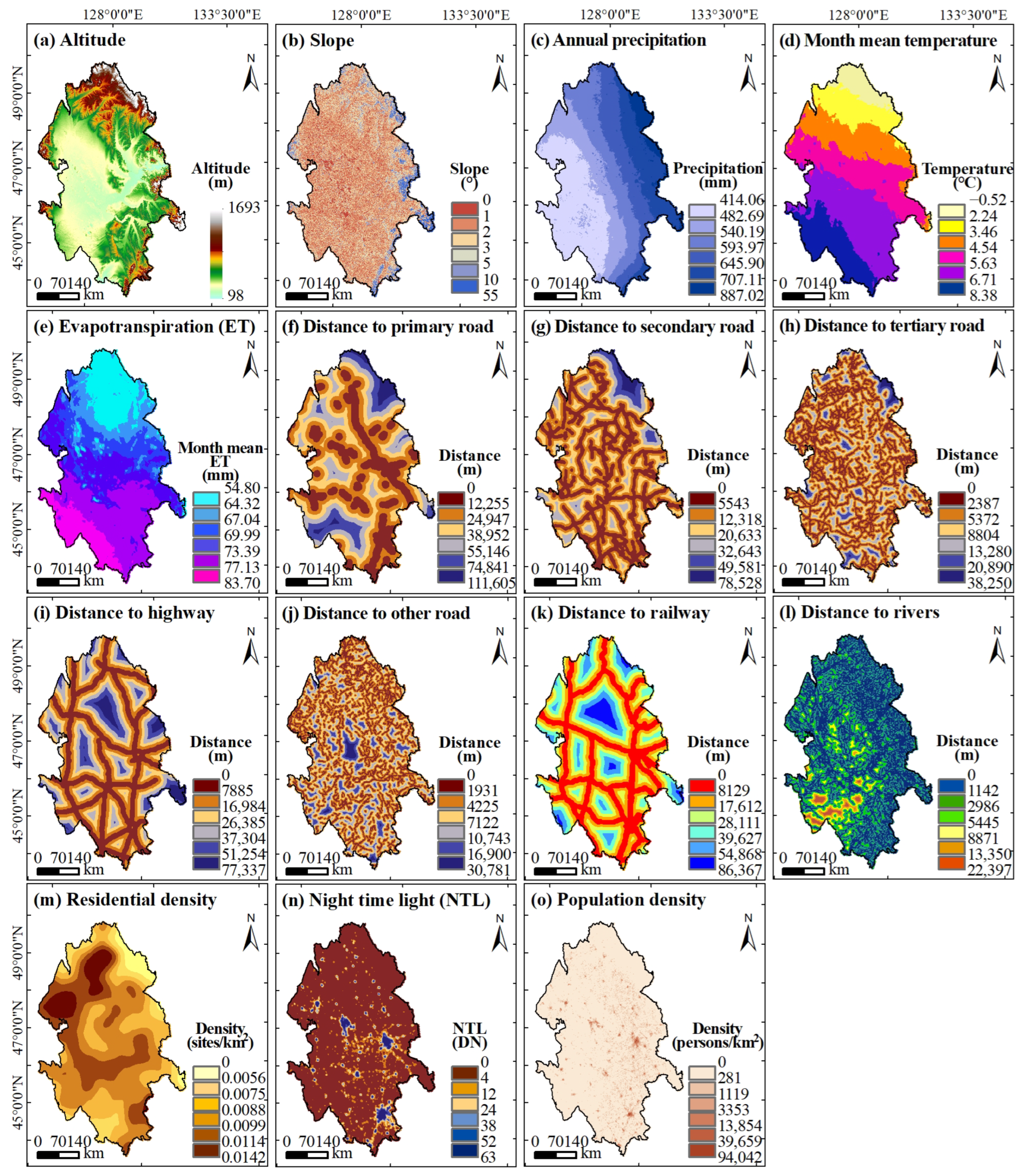
The PLUS model, developed as an enhancement of the FLUS model, is a raster-based cellular automata (CA) for simulating land dynamics and spatial allocation [12]. It integrates a rule-mining framework based on the land expansion analysis strategy (LEAS) module and a CA module utilizing multi-type random seeds (CARS). By incorporating the random forest algorithm, the model estimates the impact of various driving factors and neighborhood effects on land development and predicts the probability of land transformations under different future scenarios [14]. Driving factors employed in the PLUS model are shown in Figure 3. Model validation was conducted by comparing the simulated land use of 2020 with the observed real data. Model validation yielded an overall accuracy of 0.88, a kappa coefficient exceeding 0.80, and a Fom value of approximately 0.16, indicating strong agreement between simulated and observed land-use patterns and confirming the model’s suitability for projecting land-use changes to 2030. When running the PLUS model, the neighborhood weights of cropland, forest, grassland, water area, built-up land, bare land, and wetland are 0.21, 0.14, 0.12, 0.13, 0.12, 0.13, and 0.15, respectively. The neighborhood weight reflects the expansion tendency of a land use type driven by its own agglomeration effect: a higher weight indicates that the expansion probability of this land use type is more strongly affected by the area proportion of the same type in the surrounding neighborhood [12].
Figure 3.
Spatial distribution of 15 driving factors.
2.4. Multi-Scale Comparisons for Current and Future ES Interactions
2.4.1. Assessment of Current and Future ESs
The InVEST model (https://naturalcapitalproject.stanford.edu/software/invest, 14 June 2026), developed as a tool for mapping and valuing the services from nature that sustain and fulfill human life, was applied to estimate four key ESs under different scenarios. WY supply was assessed using the Annual Water Yield module, based on the water balance principle and adjusted according to the local water resources bulletin [7]. SR supply was quantified using the Sediment Delivery Ratio module, which estimates the value of soil retained to prevent erosion [21]. CS supply was measured using the Carbon Storage and Sequestration module, calculating the total carbon storage in above-ground (), below-ground (), soil (), and dead organic (), according to density datasets for China’s terrestrial ecosystems [28] and other relevant publications. HQ supply was measured using the Habitat Quality module, which combines the sensitivity of different land types to threat sources and the intensity of external threats [29]. Details are in Supplementary Materials Tables S1–S4.
2.4.2. Multi-Scales Calculation and Comparisons of ES Interactions
Multi-scale comparisons were conducted to identify the most appropriate spatial unit for zoning-oriented ecosystem management. An optimal scale should maximize the detection of ES interactions with sufficient magnitude and statistical significance while remaining practical for management implementation [4]. When multiple spatial scales satisfied these criteria, preference was given to larger spatial units to reduce management complexity and improve operational feasibility [8]. ES interactions were quantified using the Pearson correlation coefficient [30], where positive and negative values separately indicate synergies and trade-offs. Details can be seen in [8].
In this study, raw ES values were aggregated to each spatial scale using the arithmetic mean before analysis. Pearson correlation coefficients among ESs were calculated at four spatial scales: city, county, sub-watershed, and grid levels. Scales showing statistically significant correlations (p < 0.05) were considered suitable candidates. Among these, the scale with larger average spatial units was selected as the optimal scale for subsequent zoning analysis. Notably, Pearson correlation mainly reflects linear associations and may underestimate complex nonlinear relationships among ESs.
2.5. Dynamic ES Interaction-Based Zoning Under the Intensity–Trend–Stability Framework
2.5.1. Calculation of Three Dimensions
The proposed “intensity–trend–stability” zoning framework integrates three complementary dimensions to characterize the dynamics of ES interactions (Table 2). The first dimension represents the interaction intensity in 2020, reflecting the baseline status of ES synergies and trade-offs. The second dimension denotes the multi-scenario mean interaction intensity in 2030, indicating the projected developmental trends under future land-use conditions. The third dimension describes the consistency of interaction intensity across four 2030 scenarios, thereby reflecting the stability of future ES interaction dynamics. Following [7], interaction intensity was operationalized as trade-off intensity constrained to a range of 0–1 to ensure consistent quantitative modeling and comparability. Details can be seen in [7]. For each dimension, interaction intensity was classified into high and low levels using the regional mean value as the threshold, with values above the mean defined as high and those below the mean defined as low.
Table 2.
Description of three dimensions.
2.5.2. Ecological Zoning Based on Three Dimensions
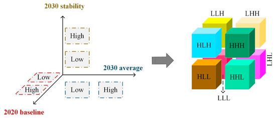
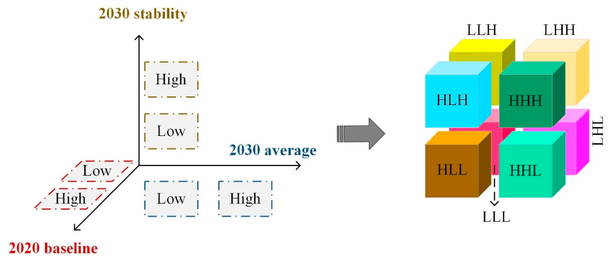
Based on this three-dimensional classification, the study area was divided into eight dynamic interaction zones (HHH, HHL, HLH, HLL, LHH, LHL, LLH, and LLL), as illustrated in Figure 4. Each letter represents the intensity level (high or low) of ES interactions in terms of baseline intensity, future trend, and scenario stability, respectively. For instance, HHH represents persistently high-intensity and stable trade-offs from 2020 to 2030, whereas LLL indicates low-intensity and unstable trade-offs. HHL denotes high baseline trade-off intensity with low stability, while LLH reflects low baseline trade-off intensity with high stability. LHH and LHL correspond to increasing trade-off intensity with stable and unstable characteristics, respectively. In contrast, HLH represents decreasing but stable trade-off intensity, and HLL indicates weakened and fluctuating trade-off intensity. By synthesizing the zoning results of the six ES pairs (i.e., WY-SR, WY-CS, WY-HQ, SR-CS, SR-HQ, and CS-HQ), this framework enables a comprehensive assessment of the spatiotemporal evolution and dominant trade-off patterns across the study region.
Figure 4.
Zoning types of the “intensity–trend–stability” ES interactions framework. The three-letter codes follow the order of 2020 baseline, 2030 average, and 2030 stability. “H” and “L” indicate high and low, respectively.
2.6. XGBoost–SHAP Analysis for ES Interactions
2.6.1. Combined Application of XGBoost and SHAP
To explore the nonlinear mechanisms driving ecosystem–service (ES) interactions, this study employed an integrated Extreme Gradient Boosting (XGBoost)–SHapley Additive exPlanations (SHAP) framework. XGBoost, a high-efficiency implementation of the gradient boosting decision tree (GBDT) algorithm [21], improves predictive performance by sequentially training multiple regression trees to iteratively correct residuals through ensemble learning. The model incorporates regularization terms into the loss function to control complexity and prevent overfitting, while first- and second-order Taylor expansions are used to optimize the objective function, thereby enhancing computational efficiency and prediction accuracy [31].
2.6.2. Parameter Configuration and Driver Selection
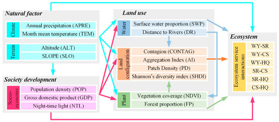
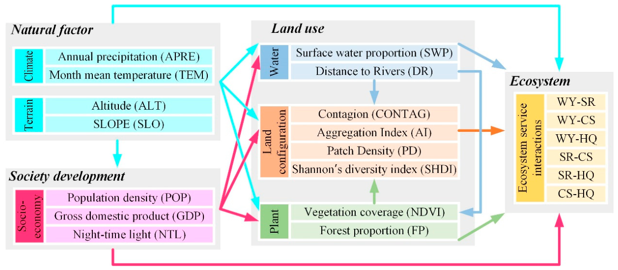
In this study, the trade-off intensity of each ES pair was used as the dependent variable, and climatic, topographic, landscape configuration, and anthropogenic factors were included as independent variables to construct XGBoost regression models. Key hyperparameters, including learning rate, maximum tree depth, number of trees, and subsampling ratio, were optimized using ten-fold cross-validation to ensure model robustness and generalization ability. To improve model interpretability, SHAP was applied to decompose model predictions into additive contributions of individual drivers based on cooperative game theory, enabling the quantification of variable importance and the identification of nonlinear response patterns and threshold effects [32]. The hypothetical influence relationships linking natural factors and anthropogenic disturbances to ES interactions are illustrated in Figure 5. To reduce the potential influence of multicollinearity, explanatory variables were pre-screened prior to model implementation, and only drivers with variance inflation factor (VIF) values lower than five were retained for subsequent XGBoost modeling. Notably, forest proportion (FP) with a VIF value of 5.36 was still kept in the model, given its critical regulatory role in shaping ES interactions. Details are in Supplementary Materials Tables S5 and S6.
Figure 5.
Hypothetical influence relationships of natural factors and anthropogenic disturbances on ES interactions.
3. Results
3.1. Spatiotemporal Changes in Land Use from 2020 to Different 2030 Scenarios
The primary land types in the Songnen Plain are cropland, forest, wetland, and grassland, which together account for over 87% of the total area, whereas water, built-up, and bare land occupy relatively small proportions (Table 3). Cropland, mainly distributed in flat regions, dominates the Songnen Plain with a high area proportion exceeding 58%. Forest is primarily concentrated around the Lesser Khingan Range and the Changbai Mountains. Wetland and grassland are mainly located in the southwestern part of the study area, where the Nenjiang and Songhua Rivers flow through (Figure 6). Compared to 2020, wetlands in all scenarios in 2030 showed an increasing trend, with the expanded proportions yielding 3.73~7.27%. In contrast, bare land decreased from 2020 to all 2030 scenarios, with reductions ranging from 634.93 to 897.38 km2. The dynamics of other land use types varied significantly across scenarios.
Table 3.
Area of land types in the Songnen Plain (km2). 1
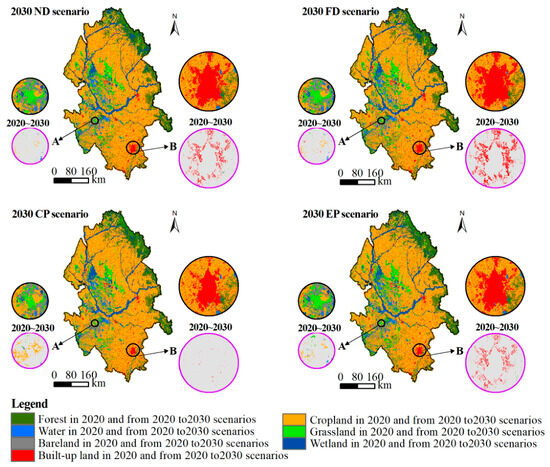
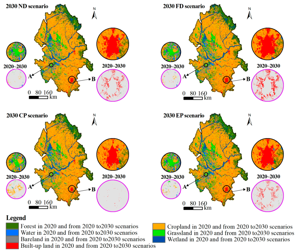
Figure 6.
Distribution and dynamics of land types from 2020 to 2030. A and B are two demo sites. Panels with black borders show the spatial distribution of land-use types under the 2030 CP scenario, while panels with purple borders display the spatial distribution of newly increased land-use types during 2020–2030.
The conversion of land use during 2020–2030 ND and 2020–2030FD are similar, presenting a “four increase, three decrease” trend. Specifically, forest, water, built-up land, and wetland are projected to increase (50.01~1329.03 km2 vs. 40.71~1306.02 km2), while cropland, grassland, and bare land are expected to decline (0.54~6.19% vs. 1.04~6.92%). Notably, the FD scenario indicates a greater potential for built-up land expansion. In the CP scenario, cropland and wetland are anticipated to increase substantially (2046.36 and 731.41 km2), accompanied by a decline in the other land types (0.05~10.55%). The EP scenario suggests future expansion of ecological land types, mainly at the expense of cropland (2692.14 km2) and built-up land (897.38 km2).
3.2. ESs Synergies and Trade-Offs from 2020 to Different 2030 Scenarios
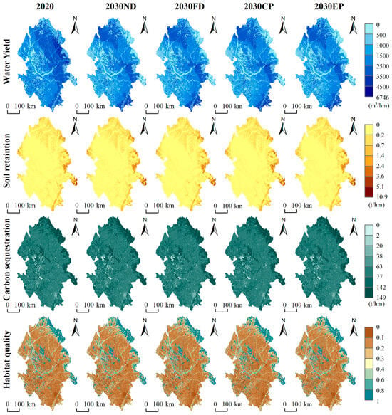
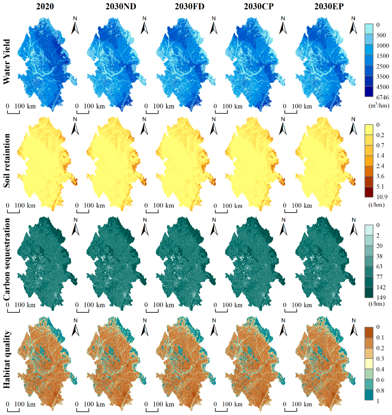
Spatial distributions of four ESs under four 2030 scenarios remain largely consistent with the baseline year 2020 (Figure 7). Distinct spatial heterogeneity is evident, with higher ES supplies predominantly occurring around the Lesser Khingan Range and the Changbai Mountains, while low supplies are mainly concentrated in the central and western plains. Temporally, variations are observed across different ESs between 2020 and the projected 2030 scenarios. The total annual supply of WY shows a declining trend (−15.25~16.55%), whereas SR exhibits a slight increase (+2.53~2.68%). Both CS and HQ are projected to decline under the 2030ND, 2030FD, and 2030CP scenarios. In contrast, the 2030EP scenario demonstrates the greatest potential for enhancing ES supply, characterized by a concurrent increase in SR, CS, and HQ.
Figure 7.
Spatial distribution of ecosystem services in 2020 and different 2030 scenarios.
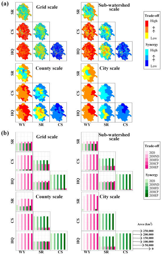
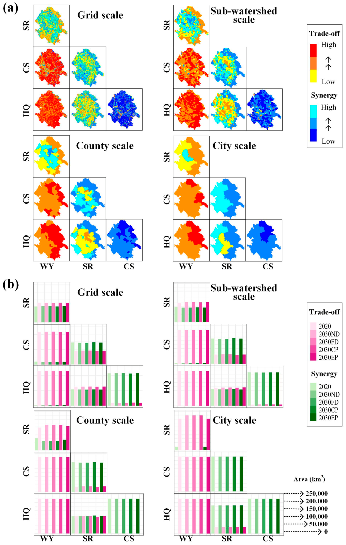
A total of six pairwise interactions among four ESs were identified for 2020 and four 2030 scenarios (Table 4, Figure 8). At the grid scale, WY exhibited consistent trade-offs with the other ESs, with the strongest negative association observed with HQ, followed by CS and SR. In contrast, SR, CS, and HQ showed significant positive correlations with each other, reflecting stable synergistic relationships. These interaction patterns remained highly consistent across all 2030 scenarios. Spatially, SR–CS and CS–HQ were dominated by synergies, with synergistic areas markedly larger than trade-offs. High levels of synergy were widely distributed across the Songnen Plain, with exceptions in mountainous, riverine, and wetland areas. Conversely, WY-related pairs were dominated by trade-offs, especially WY–CS and WY–HQ, where trade-off areas consistently exceeded synergistic areas.
Table 4.
Pearson correlation analysis of ecosystem services under future scenarios. 1
Figure 8.
Synergy and trade-off of ecosystem services: (a) spatial distribution in 2020 and (b) areas from 2020 to different 2030 scenarios.
At the sub-watershed scale, interaction patterns were largely similar to those observed at the grid scale. The trade-offs between WY and the other ESs were more pronounced in 2020 but weakened in four 2030 scenarios, whereas synergies involving SR became stronger. This highlights the tendency for regulating services to co-occur spatially, while conflicts between WY and other ESs persist.
At the county and city scales, both synergies and trade-offs weakened considerably, primarily due to the limited number of spatial units. Aggregation into larger administrative units averages out localized ecological variations, thereby diluting the strength of pairwise service interactions. Notably, interactions between WY and SR/CS even shifted direction, indicating potential scale-dependent reversals. Distinct spatial patterns were also evident at the city scale, where SR–HQ displayed a higher proportion of synergies than trade-offs, contrasting with the finer-scale results.
Summarily, correlations between ESs were consistently significant at the grid and sub-watershed scales (p < 0.01), while interaction strengths diminished at coarser administrative levels. Despite these variations, interaction patterns were broadly stable across time points and scenarios. Moreover, finer scales revealed stronger spatial heterogeneity, underscoring the importance of multi-scale perspectives in assessing ES trade-offs and synergies.
3.3. Ecological Zoning Based on Dynamic ES Interactions
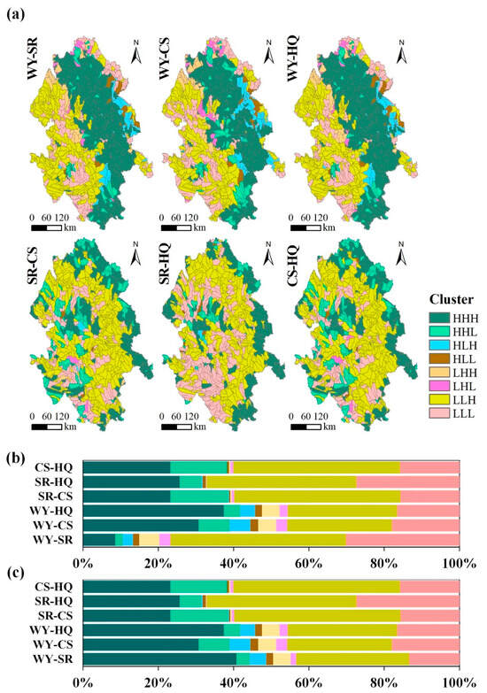
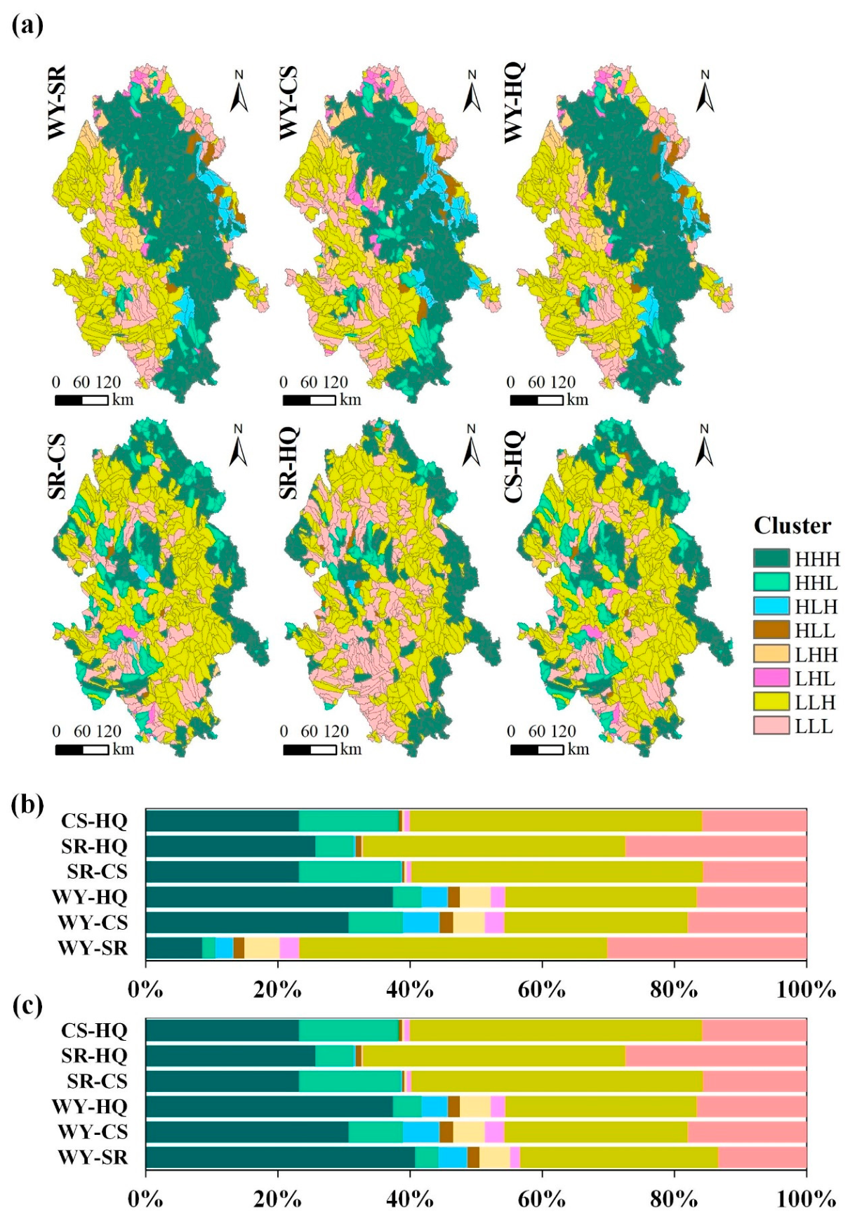
Based on the abovementioned analysis, the sub-watershed scale, which presents the most apparent spatial heterogeneity and ES interactions, was selected to employ ecological zoning. The integrated zones based on six pairs of ES interactions are shown in Figure 9. Across all six ES interaction zones, HHH and LLL were identified as the two most representative clusters. Sub-watersheds of the HHH cluster presented high-intensity and stable trade-offs that persist from 2020 to 2030, while LLL indicates low-intensity and fluctuating trade-offs. These patterns collectively reveal a distinct polarization of ecosystem–service synergies and trade-offs across the Songnen Plain. Overall, the three ES interaction zones centered on WY exhibited highly similar spatial patterns, whereas the other three interaction zones (SR-CS, SR-HQ, and CS-HQ) were spatially more consistent with one another.
Figure 9.
Integrated zones based on “intensity–trend–stability” three-dimensional ES interactions zoning framework: (a) spatial distributions, (b) percentages of sub-watershed quantities, and (c) percentages of areas.
3.3.1. Ecological Zoning Based on WY-SR, WY-CS, and WY-HQ Interactions
In the three ES interaction zones centered on WY, the HHH cluster dominated across all cases. The numbers and total areas of sub-watersheds within the WY-SR, WY-CS, and WY-HQ interaction zones are 329 (91,299.45 km2), 270 (74,891.51 km2), and 329 (91,299.45 km2), respectively, accounting for 40.76%, 33.44%, and 40.76% of the Songnen Plain. The above consistent area value is attributed to 329 overlapping sub-watersheds classified as HHH zones for both ES pairs (see Figure 9a). This indicates that WY exhibited persistently high-intensity and stable trade-offs with the other three ESs, particularly in the eastern cropland-dominated plains, where human activities are intensive.
The LLH cluster, characterized by low-intensity and stable trade-offs, ranked second, with areas of 67,161.31 km2, 63,773.06 km2, and 66,862.49 km2 across the three zones, accounting for 29.99%, 28.47%, and 29.85%, respectively. These sub-watersheds were mainly located in the western plains, also dominated by cropland and intensive cultivation. The LLL cluster, reflecting low-intensity but fluctuating trade-offs, was mainly distributed in wetland–grassland ecotones and partially in eastern mountainous regions, with areas of 29,939.96 km2, 35,041.14 km2, and 30,238.78 km2, accounting for 13.37%, 15.65%, and 13.50%, respectively. Collectively, LLH and LLL clusters covered more than one-third of the Songnen Plain, indicating that large areas of the Songnen Plain were under weak trade-offs and relatively strong synergies among ESs, suggesting limited anthropogenic disturbance.
In contrast, transitional clusters such as HLH (decreasing but stable trade-off intensity) and LHL (enhanced but fluctuating trade-offs) occupied smaller, fragmented regions along ecological transition zones and terrain gradients. Benefiting from a good initial eco-environment, HLH regions witness a gradual reduction in trade-off strength driven by long-term agricultural water exploitation; in contrast, LHL areas start with weak ES interactions, and future farmland expansion elevates trade-off intensity, accompanied by prominent fluctuation. Such transitional mosaics are sensitive to land and water management policies and serve as key priority zones for wetland restoration and cropland optimization.
3.3.2. Ecological Zoning Based on SR-CS, SR-HQ, and CS-HQ Interactions
In the three ES interaction zones involving SR, CS, and HQ, the LLH and LLL clusters were predominant.
The LLH cluster, representing low-intensity and stable trade-offs, included 388 (101,803.10 km2), 349 (96,797.23 km2), and 389 (103,065.87 km2) sub-watersheds for the SR-CS, SR-HQ, and CS-HQ zones, accounting for 45.45%, 43.22%, and 46.02% of the Songnen Plain, respectively. These results indicate that most sub-watersheds remained in a stable low-intensity trade-off state across time and scenarios, implying significant synergistic effects among these ESs.
The LLL cluster consisted of 138, 241, and 139 sub-watersheds, covering 33,303.99 km2, 62,094.20 km2, and 33,350.02 km2, which represent 14.87%, 27.72%, and 14.89% of the study area, respectively. These clusters were mostly distributed across flat plains and wetland-dominated regions.
Conversely, the HHH cluster comprised 204, 226, and 204 sub-watersheds, with total areas of 52,561.93 km2, 53,439.17 km2, and 52,736.88 km2, corresponding to 23.47%, 23.86%, and 23.55% of the study area. These zones were mainly concentrated in mountainous regions with dense vegetation, such as the Lesser Khingan Mountains and Changbai Mountains.
Transitional clusters such as HLH and LHL patches mainly gather at the mountain–plain foothill transition zone. HLH units with high baselines but descending trade-offs are dominated by marginally degraded forestland; LHL zones with rising and volatile interactions arise from fragmented land conversion between mountain woodland and plain cropland. Due to their high variability in future ES evolution, these unstable HLH and LHL areas are pinpointed as crucial intervention zones for afforestation and scattered cultivated land consolidation.
Overall, these findings demonstrate that ecological restoration and conservation measures have effectively mitigated competition among soil retention, carbon sequestration, and habitat quality, thereby enhancing their synergistic relationships. The consistent spatial behavior of these interactions suggests the existence of shared ecological driving mechanisms among the three ES pairs.
3.4. Drivers of ES Interactions in the Songnen Plain
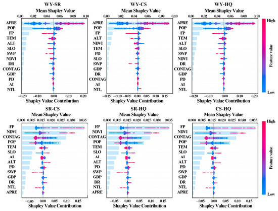
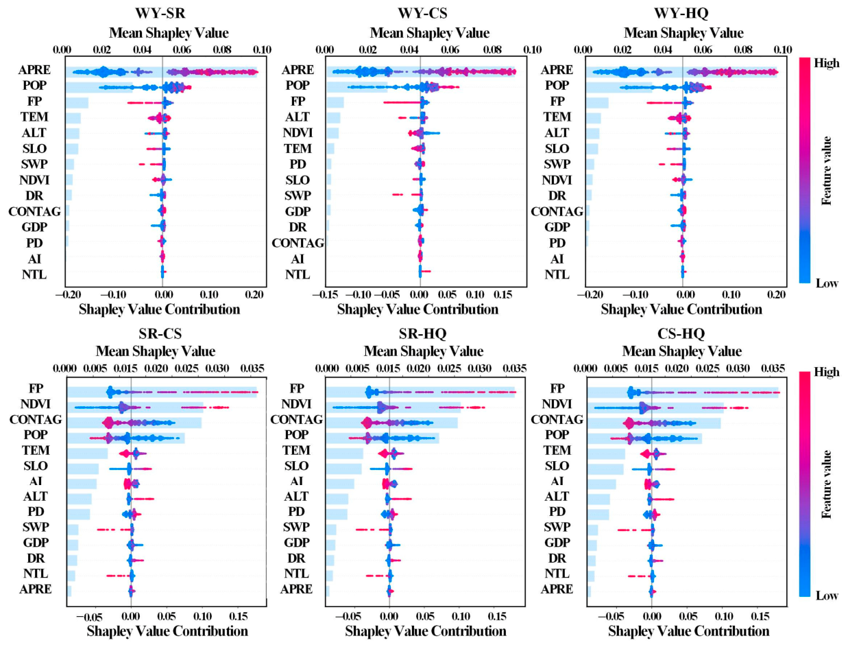
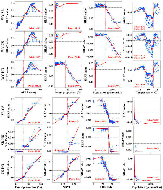
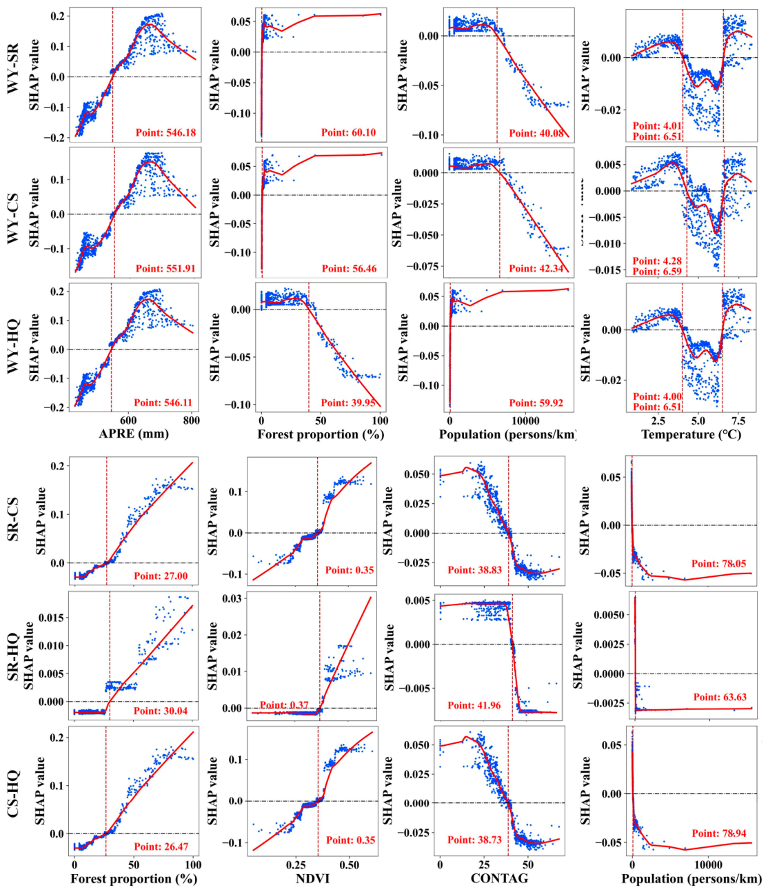
For the three ES interactions centered on WY, APRE emerged as the most influential driver, exhibiting consistently positive correlations with WY-SR, WY-CS, and WY-HQ interactions (Figure 10). This suggests that increases in precipitation are associated with strengthened ES interactions involving WY. POP, FP, TEM, ALT, and SLO followed in importance. Among the 14 drivers, POP, DR, CONTAT, and AI showed positive correlations with all three WY-centered interactions, whereas the remaining ones exhibited significant negative effects. A notable distinction was observed for the WY-CS interaction, where NDVI exerted a stronger negative influence than TEM, SLO, and SWP, indicating that vegetation conditions played a comparatively larger constraining role in this specific interaction. Overall, these findings highlight that climate and topography contributed more prominently to the WY-centered ES interactions than human disturbances. A noteworthy phenomenon is that TEM demonstrated a “nonlinear dual-threshold effect” on all three interactions involving WY. Specifically, when the annual average temperature is below 4.0 °C, rising temperature improves vegetation growth and water retention capacity, further promoting the synergy among paired ecosystem services; when temperature exceeds 4.0 °C and continues increasing up to around 6.5 °C, accelerated evapotranspiration gradually consumes regional available water resources, which shifts the temperature’s effect from positive promotion to negative inhibition on ES interactions. This implies that when the TEM deviates significantly from the optimal range, the synergistic relationship between ecological processes might be disrupted. Figure 11 shows the nonlinear effects of several selected drivers on ES interactions in detail.
Figure 10.
The summary plot of the SHAP value for ES interactions. The rank of features represents the relative importance. The bar represents the mean |SHAP| values of features, corresponding to the top x-axis. The bee swarm plot represents the distribution of SHAP values of samples, corresponding to the bottom x-axis, with the color and vertical distribution representing the feature value magnitude and density of samples. Red indicates high feature values; blue indicates low feature values.
Figure 11.
The dependence plots for ES interactions. The scatter depicts the change in SHAP values along the gradient of feature value. The zero line distinguishes the positive and negative driving forces of the corresponding features. The polynomial curve fitted by the Loess method was utilized for smoothing the series. Texts in red indicate the key thresholds of each driving factor.
For the ES interactions among the SR, CS, and HQ (i.e., SR-CS, SR-HQ and CS-HQ), the 14 drivers exhibited broadly similar influences. Vegetation conditions, represented by FP and NDVI, made the largest contributions to these interactions, followed by CONTAG, POP, TEM, SLO, AI, ALT, and PD. This pattern underscores the relatively high importance of landscape structure and topography in regulating these ES interactions. Positive effects were consistently observed for FP, NDVI, SLO, ALT, PD, DR, and APRE, whereas the remaining factors exerted negative influences. Similar to the WY-centered interactions, the “nonlinear dual-threshold effect” of TEM was also evident in these ES relationships.
4. Discussion
4.1. Scenario-Driven Land-Use Change and ES Responses
Our results demonstrate that land-use trajectories under alternative development scenarios substantially influence the magnitude of ES changes, while the direction of ES interactions remains relatively stable. Across all scenarios, wetlands expanded and bare land declined, suggesting an overall improvement in ecological conditions in the Songnen Plain. This trend is consistent with recent observations of land-use dynamics in the region [33] and likely reflects the cumulative effects of ecological restoration programs, strengthened wetland protection policies, and degraded land rehabilitation initiatives [34].
By contrast, cropland and built-up land exhibited strong scenario dependency, highlighting the role of policy priorities in shaping land-use outcomes. Development-oriented scenarios promoted urban expansion at the expense of cropland, whereas ecological protection strategies significantly increased ecological land, as echoed by [21]. These differences translated into distinct ES responses: WY declined under all scenarios, SR increased slightly, and CS and HQ declined under development-oriented pathways but improved under ecological protection scenarios. Similar patterns have been reported in other scenario-based ES studies [22], emphasizing the sensitivity of regulating and supporting services to land-use strategies.
Despite these differences in ES magnitude, the intrinsic interactive structure among ESs remains steady. WY inherently constrains other ESs and forms persistent trade-off relations, while SR, CS, and HQ possess mutually promotive functional attributes and present stable synergies. Essentially, policy adjustments and land development strategies only exert quantitative impacts on service supply capacity but cannot alter the intrinsic functional correlation nature. Accordingly, coordinated assessment of multiple ecosystem services is required in regional land management to mitigate ecological risks caused by one-sided governance.
Despite these differences in ES magnitude, the structure of ES interactions showed remarkable consistency across scenarios. WY consistently exhibited trade-offs with other services, whereas SR, CS, and HQ maintained predominantly synergistic relationships. This finding suggests that interaction directions are largely governed by underlying land-use transitions and ecosystem processes rather than by individual scenario assumptions. The coexistence of persistent trade-offs and stable synergies underscores the importance of jointly evaluating multiple ESs in regional planning to avoid unintended ecological consequences.
Spatial scale further shapes the detection and interpretation of ES interactions. Consistent with previous studies [17], finer spatial resolutions revealed stronger and more explicit trade-offs and synergies, whereas coarser scales tended to obscure local heterogeneity through spatial aggregation. Although grid-based analysis captured the most pronounced interaction signals, its direct application in management remains limited due to operational complexity [8]. In contrast, sub-watersheds represent a practical compromise, as they reflect hydrological and ecological processes while remaining suitable for spatial planning and management implementation [7]. These findings highlight the importance of aligning analytical scales with ecological processes and governance structures when translating ES assessments into policy-relevant zoning strategies. Notably, sub-basin boundaries cannot fully match administrative divisions, which underscores the necessity of a dual-dimensional selection framework balancing ecological integrity and administrative practicability to guide scale determination for future regional studies.
4.2. Advancing ES Interaction Zoning Under Future Uncertainty
4.2.1. A Dynamic Framework for Identifying Robust Interaction Regimes
Building on the observed scenario- and scale-dependent ES interaction patterns, this study proposes a three-dimensional “intensity–trend–stability” framework to support dynamic zoning of ES interaction. Unlike conventional approaches that rely on static assessments or single-scenario projections [25], our framework simultaneously integrates current interaction intensity, future trajectories, and cross-scenario robustness. This design enables a more comprehensive representation of ES interactions under uncertainty and supports forward-looking ecosystem management.
Consistent with existing watershed-scale ES theories, this study also verifies the universal functional differentiation of ES interactions: WY tends to form trade-offs with other services, while vegetation-related regulating services maintain mutual synergies. These core spatial patterns are consistent with prior empirical findings [7]. These patterns reflect fundamental differences in underlying ecological mechanisms. Nevertheless, most previous studies only classified ES zones based on static single-period intensity and ignored temporal trends and scenario stability, failing to identify fluctuating transitional zones and lacking future-oriented zoning capacity. Targeting these gaps, our framework improves existing methods by adding trend and stability dimensions, which enable dynamic classification of stable conflict zones, synergistic hotspots, and policy-sensitive transitional regions.
More importantly, the proposed framework extends ES interaction zoning beyond simple pattern identification. By jointly evaluating interaction intensity, temporal trends, and scenario stability, it distinguishes three types of management-relevant interaction regimes, i.e., persistent conflict zones, robust synergistic hotspots, and policy-sensitive transitional areas. Persistent high-conflict zones (sub-watersheds classified as HHH and HLH) represent locations where trade-offs are strong and stable across scenarios, requiring careful balancing of ecosystem functions. In contrast, synergistic hotspots (LLH and HLH) provide opportunities for multi-benefit ecosystem management, while transitional areas (HHL, LHL, HLL, and LHH) remain highly sensitive to land-use policies and therefore represent priority zones for adaptive intervention. Through this classification, the framework provides a dynamic and uncertainty-aware basis for ecological zoning and decision-making. This zoning scheme provides clear guidance for differentiated land management. Persistent high-conflict zones require strict land-use regulation and targeted ecological restoration to mitigate ES trade-offs. Robust synergistic hotspots should be steadily protected to maintain multi-service ecological benefits. Policy-sensitive transitional areas necessitate dynamic monitoring and adaptive governance to avoid the degradation of ES synergies. Such zone-based strategies support refined spatial governance and balance regional ecological conservation and socioeconomic development.
4.2.2. Mechanistic Insights from Interpretation Machine Learning
Understanding the drivers of ES interactions is essential for translating spatial patterns into actionable management strategies. The integration of XGBoost and SHAP provides a mechanism-oriented perspective by identifying dominant drivers, nonlinear responses, and critical thresholds shaping ES interactions.
Consistent with existing ecological cognition [7], our results confirm divergent driving rules across different ES combinations: climatic and topographic conditions dominate trade-offs associated with WY, whereas vegetation and landscape features primarily determine synergies among SR, CS, and HQ. This separation originates from disparate biophysical constraints on hydrological versus vegetation-dependent ecosystem functions. Whereas most prior machine-learning-based ES research only screens influential variables qualitatively, our study delivers two incremental improvements: we quantitatively detect the dual nonlinear thresholds of key climatic factors via SHAP dependence curves and further quantify relative importance to separate natural topo-climatic drivers from anthropogenic interference.
The SHAP analysis further reveals pronounced nonlinear responses and threshold effects, particularly for temperature-related variables, which underscore the sensitivity of ES interactions to climatic extremes. Moderate increases in water availability tend to enhance vegetation growth, soil retention, and habitat conditions simultaneously, reinforcing synergies among regulating services. However, beyond certain thresholds, increased vegetation water demand may intensify evapotranspiration, thereby strengthening trade-offs between WY and other services. These results highlight the importance of considering vegetation–hydrology coupling and nonlinear climate responses when designing ecosystem restoration or land-use optimization strategies. This nonlinear transition and threshold effect is an inherent feature of regional eco-hydrological systems. Within favorable hydrothermal ranges, vegetation and hydrological processes operate synergistically to sustain balanced ES relationships. Once crossing ecological tipping points, the coupled vegetation–water system becomes unbalanced, triggering abrupt shifts between ES trade-offs and synergies. This also explains why conventional linear models are limited in capturing complex ES interaction rules.
Interestingly, the relatively stronger contributions of climatic and topographic factors compared to anthropogenic variables suggest that natural environmental gradients remain the primary determinants of spatial heterogeneity in ES interactions across the Songnen Plain. From a management perspective, this implies that policy interventions should be tailored to underlying biophysical constraints rather than relying solely on uniform land-use regulations.
4.3. Limitations and Future Research Directions
Although developed using the Songnen Plain as a case study, the proposed framework has potential applicability to other regions characterized by land-use change and ecosystem service trade-offs. Nevertheless, several limitations should be acknowledged. First, uncertainties remain in the future land-use simulations. Although four contrasting scenarios were designed to represent plausible development pathways, their parameterization inevitably simplifies complex socioeconomic processes, policy adjustments, and unexpected disturbances. The standardized ±15% adjustment adopted in this study was intended to ensure comparability among scenarios and to systematically evaluate the effects of different development priorities on ecosystem service (ES) interactions. However, this setting does not necessarily reflect the actual magnitude of policy interventions for different land-use types. In addition, no formal sensitivity analysis was conducted for key PLUS model parameters. Consequently, future land-use trajectories may differ from the simulated outcomes, introducing uncertainty into subsequent ES assessments.
Second, uncertainties are also associated with ES quantification. The InVEST model relies on simplified ecological processes and parameter assumptions that may not fully capture local environmental heterogeneity and fine-scale ecological dynamics. Moreover, model outputs were not validated using field observations because of data limitations. For the 2030 simulations, only land-use patterns were updated under different scenarios, whereas climatic and other environmental variables were maintained at their 2020 baseline conditions. This design follows common practice in land-use scenario studies and allows the isolated effects of land-use change on ESs to be evaluated. Nevertheless, it neglects potential impacts of future environmental change, particularly for climate-sensitive services such as water yield and soil retention. Beyond this, we adopted the regional mean value as the dichotomy threshold to classify high and low ES interaction intensity, trend, and stability. This artificial threshold selection is a methodological choice, and shifting the cutoff may alter the area proportion of the eight zoning clusters.
Third, the proposed framework involves a sequential integration of the PLUS model, the InVEST model, and the XGBoost–SHAP analysis. As in most multi-model studies, uncertainties originating from individual models may accumulate and propagate through the modeling chain, potentially affecting the final zoning results. Furthermore, the classification of interaction intensity, trend, and stability was based on regional mean values. Although this approach provides a straightforward and interpretable zoning scheme, alternative threshold settings may yield different spatial patterns.
Future research should focus on improving the robustness and realism of dynamic ES interaction assessments. More flexible scenario frameworks, such as policy-constrained, data-driven, or stochastic simulations, could better capture socioeconomic uncertainties and evolving policy processes. Differentiated transition adjustments based on empirical policy targets may further improve future land-use scenario design. In addition, incorporating dynamically changing climate (e.g., CMIP6), soil, and socioeconomic variables, together with higher-resolution and multi-source remote sensing products, would enhance the realism of both land-use and ES simulations. Finally, systematic sensitivity analyses, field-based validation, uncertainty propagation assessment, and alternative zoning thresholds should be explored to strengthen the reliability and transferability of the proposed framework for long-term ecosystem management and sustainable land-use planning.
5. Conclusions
This study establishes an integrated analytical framework to uncover the spatiotemporal dynamics, driving mechanisms of ES interactions, and corresponding ecological zoning patterns across multiple future land-use scenarios on the Songnen Plain. Core findings indicate that land-use conversions from 2020 to 2030 vary notably under distinct development scenarios: wetland consistently expands, and bare land shrinks universally, while cropland and built-up land changes are highly sensitive to targeted land management policies. Regulating and supporting services were advantaged under ecological protection scenarios. Across all scenarios, stable trade-offs between WY and other services, alongside strong synergies among SR, CS, and HQ, reflected fundamental ES functional differences. The proposed “intensity–trend–stability” framework integrates historical features and future trends to distinguish stable conflicting zones, synergistic hotspots, and transitional regions. It surpasses static classification methods and holds potential transferability for similar regional studies. XGBoost–SHAP model further clarifies divergent driving rules: climatic and topographic attributes predominantly govern interactions relevant to WY, whereas vegetation status and landscape configuration determine synergies among SR, CS, and HQ, accompanied by widespread nonlinear threshold responses. Overall, this study deepens the understanding of ES interaction dynamics and provides useful scientific references for scale-based ecological zoning and differentiated management strategies. The proposed framework is applicable to other ecologically sensitive and policy-driven regions, supporting sustainable land-use planning that balances ecological protection and socioeconomic development.
Supplementary Materials
The following supporting information can be downloaded at: https://www.mdpi.com/article/10.3390/rs18122014/s1. Table S1: Parameters used in InVEST model for assessing water yield (WY); Table S2: Parameters used in InVEST model for assessing soil retention (SR); Table S3: Parameters used in InVEST model for assessing carbon sequestration (CS); Table S4: Parameters used in InVEST model for assessing habitat quality (HQ); Table S5: The optimal parameters for XGBoost models; Table S6: The validation of XGBoost models; Table S7: The VIFs and tolerances of variables applied to XGBoost models; Table S8: Top three driving factors for each ES interaction pair, ranked by mean absolute SHAP value; Table S9: Transition matrix of four scenarios for conducting the PLUS model; Table S10: Spearman correlation analysis of ecosystem services under future scenarios; Table S11: Statistics of three indicators of ecological zones.
Author Contributions
Conceptualization, S.Y.; methodology, S.Y., Z.T. and J.H.; software, S.Y.; validation, Z.T., L.Y., A.J. and S.C.; formal analysis, S.Y. and J.H.; investigation, Z.T., L.Y., A.J. and S.C.; resources, S.Y.; data curation, S.Y.; writing—original draft preparation, S.Y.; writing—review and editing, S.Y., L.Y., S.C. and K.J.; visualization, S.Y. and J.H.; supervision, K.J.; project administration, S.Y. and K.J.; funding acquisition, S.Y. and K.J. All authors have read and agreed to the published version of the manuscript.
Funding
This research was funded by the Fundamental Research Funds of CAF, grant number CAFYBB2023ZA004 and CAFYBB2024QD001-04.
Data Availability Statement
The land use and cover datasets were obtained from the Chinese Academy of Sciences. The climate datasets were obtained from the National Earth System Science Data Center (https://www.geodata.cn/, accessed on 11 December 2025). The geography datasets were obtained from the National Catalogue Service for Geographic Information (https://www.webmap.cn, accessed on 11 December 2025). The soil datasets were obtained from the World Soil Information (https://www.isric.org/, accessed on 12 October 2024). The population density from the WorldPop Platform (https://hub.worldpop.org/, accessed on 11 December 2025). The generated ecosystem service products will be made available on request.
Conflicts of Interest
The authors declare no conflicts of interest.
Abbreviations
The following abbreviations are used in this manuscript:
| ES | Ecosystem services | APRE | Annual precipitation |
| WY | Water yield | TEM | Monthly mean temperature |
| SR | Soil retention | GDP | Gross domestic product |
| CS | Carbon sequestration | NTL | Night-time light |
| HQ | Habitat quality | SWP | Surface water proportion |
| ALT | Altitude | CONTAG | Contagion |
| SLO | Slope | AI | Aggregation index |
| FP | Forest proportion | PD | Patch density |
| POP | Population density | SHDI | Shannon’s diversity index |
| DR | Distance to rivers | NDVI | Normalized difference vegetation index |
References
- Boyd, J.; Banzhaf, S. What Are Ecosystem Services? The Need for Standardized Environmental Accounting Units. Ecol. Econ. 2007, 63, 616–626. [Google Scholar] [CrossRef] [Scilit]
- Costanza, R.; De Groot, R.; Sutton, P.; Van Der Ploeg, S.; Anderson, S.J.; Kubiszewski, I.; Farber, S.; Turner, R.K. Changes in the Global Value of Ecosystem Services. Glob. Environ. Change 2014, 26, 152–158. [Google Scholar] [CrossRef] [Scilit]
- Wu, Q.; Jiang, X.; Song, M.; Liu, Y.; Shi, X.; Lei, Y.; Nie, T. Study on the Development Trend of Social-Ecological Systems and the Drivers of Sustainable Development—A Case Study of the Loess Plateau in China. Ecol. Indic. 2023, 156, 111172. [Google Scholar] [CrossRef] [Scilit]
- Yin, D.; Yu, H.; Shi, Y.; Zhao, M.; Zhang, J.; Li, X. Matching Supply and Demand for Ecosystem Services in the Yellow River Basin, China: A Perspective of the Water-Energy-Food Nexus. J. Clean. Prod. 2023, 384, 135469. [Google Scholar] [CrossRef] [Scilit]
- Yang, Q.; Qian, H.; Gao, Y.; Duan, Y.; Cao, Z.; Tian, P.; Li, K.; Yang, S.; Zhao, W.; Long, Q. Spatio-Temporal Evolution and Driving Mechanism of Ecosystem Services in Typical Hilly and Gully Areas of the Loess Plateau: A Case Study in Yan’an Region, Shaanxi Province. Ecol. Indic. 2025, 177, 113773. [Google Scholar] [CrossRef] [Scilit]
- Shifaw, E.; Sha, J.; Li, X.; Bao, Z.; Ji, J.; Ji, Z.; Kassaye, A.Y.; Lai, S.; Yang, Y. Ecosystem Services Dynamics and Their Influencing Factors: Synergies/Tradeoffs Interactions and Implications, the Case of Upper Blue Nile Basin, Ethiopia. Sci. Total Environ. 2024, 938, 173524. [Google Scholar] [CrossRef] [Scilit] [PubMed]
- Huang, J.; Yu, S.; Chen, J.; Githaiga, K.B.; Njuguna, S.M.; Yan, X. Rainfall Cycle Causes the Inter-Seasonal Instability of Ecosystem Service Trade-Offs: A Case Study in the Tana River Basin, Kenya. J. Clean. Prod. 2024, 478, 143956. [Google Scholar] [CrossRef] [Scilit]
- Yu, S.; Huang, J.; Cai, S.; Ju, H.; Jiang, A.; Chen, J.; Jin, K. Linking Scale-Dependent Ecosystem Service Interactions with Driver-Based Zoning Strategies: A Case Study of the Songnen Plain. Ecol. Eng. 2026, 225, 107902. [Google Scholar] [CrossRef] [Scilit]
- Xu, H.; Zhao, C.; Chen, S.; Shan, S.; Qi, X.; Chen, T.; Wang, X. Spatial Relationships among Regulating Ecosystem Services in Mountainous Regions: Nonlinear and Elevation-Dependent. J. Clean. Prod. 2022, 380, 135050. [Google Scholar] [CrossRef] [Scilit]
- Bradford, J.B.; D’Amato, A.W. Recognizing Trade-offs in Multi-objective Land Management. Front. Ecol. Environ. 2012, 10, 210–216. [Google Scholar] [CrossRef] [Scilit]
- Baude, M.; Meyer, B.C.; Schindewolf, M. Land Use Change in an Agricultural Landscape Causing Degradation of Soil Based Ecosystem Services. Sci. Total Environ. 2019, 659, 1526–1536. [Google Scholar] [CrossRef] [Scilit] [PubMed]
- Liang, X.; Guan, Q.; Clarke, K.C.; Liu, S.; Wang, B.; Yao, Y. Understanding the Drivers of Sustainable Land Expansion Using a Patch-Generating Land Use Simulation (PLUS) Model: A Case Study in Wuhan, China. Comput. Environ. Urban Syst. 2021, 85, 101569. [Google Scholar] [CrossRef] [Scilit]
- Liu, X.; Liang, X.; Li, X.; Xu, X.; Ou, J.; Chen, Y.; Li, S.; Wang, S.; Pei, F. A Future Land Use Simulation Model (FLUS) for Simulating Multiple Land Use Scenarios by Coupling Human and Natural Effects. Landsc. Urban Plan. 2017, 168, 94–116. [Google Scholar] [CrossRef] [Scilit]
- Rong, T.; Qin, M.; Zhang, P.; Chang, Y.; Liu, Z.; Zhang, Z. Spatiotemporal Evolution of Land Use Carbon Emissions and Multi Scenario Simulation in the Future-Based on Carbon Emission Fair Model and PLUS Model. Environ. Technol. Innov. 2025, 38, 104087. [Google Scholar] [CrossRef] [Scilit]
- Hou, W.; Hu, T.; Yang, L.; Liu, X.; Zheng, X.; Pan, H.; Zhang, X.; Xiao, S.; Deng, S. Matching Ecosystem Services Supply and Demand in China’s Urban Agglomerations for Multiple-Scale Management. J. Clean. Prod. 2023, 420, 138351. [Google Scholar] [CrossRef] [Scilit]
- Li, Y.; Geng, H.; Luo, G.; Wu, L.; Wang, J.; Wu, Q. Multiscale Characteristics of Ecosystem Service Value Trade-Offs/Synergies and Their Response to Landscape Pattern Evolution in a Typical Karst Basin in Southern China. Ecol. Inform. 2024, 81, 102584. [Google Scholar] [CrossRef] [Scilit]
- Dang, L.; Zhao, F.; Teng, Y.; Teng, J.; Zhan, J.; Zhang, F.; Liu, W.; Wang, L. Scale Dependency of Trade-Offs/Synergies Analysis of Ecosystem Services Based on Bayesian Belief Networks: A Case of the Yellow River Basin. J. Environ. Manag. 2025, 375, 124410. [Google Scholar] [CrossRef] [Scilit] [PubMed]
- Xu, X.; Wang, C.; Sun, Z.; Hao, Z.; Day, S. How Do Urban Forests with Different Land Use Histories Influence Soil Organic Carbon? Urban For. Urban Green. 2023, 83, 127918. [Google Scholar] [CrossRef] [Scilit]
- Li, X.; Zhou, W. Optimizing Urban Greenspace Spatial Pattern to Mitigate Urban Heat Island Effects: Extending Understanding from Local to the City Scale. Urban For. Urban Green. 2019, 41, 255–263. [Google Scholar] [CrossRef] [Scilit]
- Jiang, A.; Sun, F.; Zhang, B.; Wu, Q.; Cai, S.; Yang, Z.; Chang, Y.; Han, R.; Yu, S. Spatiotemporal Dynamics and Driving Factors of Vegetation Coverage around Linear Cultural Heritage: A Case Study of the Beijing-Hangzhou Grand Canal. J. Environ. Manag. 2024, 349, 119431. [Google Scholar] [CrossRef] [Scilit] [PubMed]
- Wang, H.; Zhang, C.; Yao, X.; Yun, W.; Ma, J.; Gao, L.; Li, P. Scenario Simulation of the Tradeoff between Ecological Land and Farmland in Black Soil Region of Northeast China. Land Use Policy 2022, 114, 105991. [Google Scholar] [CrossRef] [Scilit]
- Lu, Z.; Li, C.; Zhang, J.; Lei, G.; Yu, Z.; Dong, Z. Impact of Land Use Change on Actual Evapotranspiration in the Songnen Plain, China. J. Hydrol. Reg. Stud. 2024, 54, 101854. [Google Scholar] [CrossRef] [Scilit]
- Sun, G.; Chen, Y.; Bi, X.; Yang, W.; Chen, X.; Zhang, B.; Cui, Y. Geochemical Assessment of Agricultural Soil: A Case Study in Songnen-Plain (Northeastern China). CATENA 2013, 111, 56–63. [Google Scholar] [CrossRef] [Scilit]
- Wang, S.; Shi, H.; Xu, X.; Huang, L.; Gu, Q.; Liu, H. County Zoning and Optimization Paths for Trade-Offs and Synergies of Ecosystem Services in Northeast China. Ecol. Indic. 2024, 164, 112044. [Google Scholar] [CrossRef] [Scilit]
- NASA JPL. NASADEM Merged DEM Global 1 Arc Second V001 [Data Set]. NASA EOSDIS Land Processes DAAC. 2020. Available online: https://www.earthdata.nasa.gov/data/catalog/lpcloud-nasadem-hgt-001 (accessed on 1 January 2025).
- Wu, Y.; Shi, K.; Chen, Z.; Liu, S.; Chang, Z. Developing Improved Time-Series DMSP-OLS-Like Data (1992–2019) in China by Integrating DMSP-OLS and SNPP-VIIRS. IEEE Trans. Geosci. Remote Sens. 2022, 60, 4407714. [Google Scholar] [CrossRef] [Scilit]
- Yan, F.; Shangguan, W.; Zhang, J.; Hu, B. Depth-to-Bedrock Map of China at a Spatial Resolution of 100 Meters. Sci. Data 2020, 7, 2. [Google Scholar] [CrossRef] [Scilit] [PubMed]
- Xu, L.; He, N.; Yu, G. A Dataset of Carbon Density in Chinese Terrestrial Ecosystems (2010s). China Sci. Data 2019, 4, 90–96. [Google Scholar] [CrossRef] [Scilit]
- Zheng, L.; Wang, Y.; Li, J. Quantifying the Spatial Impact of Landscape Fragmentation on Habitat Quality: A Multi-Temporal Dimensional Comparison between the Yangtze River Economic Belt and Yellow River Basin of China. Land Use Policy 2023, 125, 106463. [Google Scholar] [CrossRef] [Scilit]
- Campbell, R.C.; Sokal, R.R.; Rohlf, F.J. Biometry: The Principles and Practice of Statistics in Biological Research. J. R. Stat. Society. Ser. A (Gen.) 1970, 133, 102. [Google Scholar] [CrossRef] [Scilit]
- Sun, D.; Wu, X.; Wen, H.; Ma, X.; Zhang, F.; Ji, Q.; Zhang, J. Ecological Security Pattern Based on XGBoost-MCR Model: A Case Study of the Three Gorges Reservoir Region. J. Clean. Prod. 2024, 470, 143252. [Google Scholar] [CrossRef] [Scilit]
- Huang, J.; Yu, S.; Njuguna, S.M.; Onyango, J.; Githaiga, K.B.; Ling, F.; Yan, X. Improving Water-Carbon Coupling under Seasonal Hydroclimatic Variability: Exploring Water Use Efficiency and Its Seasonal Aridity Resilience in the Tana River Basin, Kenya. J. Hydrol. Reg. Stud. 2025, 62, 103001. [Google Scholar] [CrossRef] [Scilit]
- Feng, L.; Yu, Z.; Lei, G. Ecosystem Services in the Typical Black Soil Region of Northeastern China: Implications for the Optimal Land Use Pattern. Environ. Dev. Sustain. 2024, 27, 19241–19264. [Google Scholar] [CrossRef] [Scilit]
- Luo, L.; Wang, X.; Wang, Z. Identifying Variations in Ecosystem Health of Wetlands in the Western Songnen Plain (2000–2020). Water 2025, 17, 3175. [Google Scholar] [CrossRef] [Scilit]

Disclaimer/Publisher’s Note: The statements, opinions and data contained in all publications are solely those of the individual author(s) and contributor(s) and not of MDPI and/or the editor(s). MDPI and/or the editor(s) disclaim responsibility for any injury to people or property resulting from any ideas, methods, instructions or products referred to in the content. |
© 2026 by the authors. Licensee MDPI, Basel, Switzerland. This article is an open access article distributed under the terms and conditions of the Creative Commons Attribution (CC BY) license.