Seasonal and Diurnal Variations of Wind Fields, Low-Level Jets, and Mixing-Layer Height over Beijing Based on One-Year Doppler Wind Lidar Observations

Highlights

What are the main findings?

• One year of Doppler wind lidar observations at an urban Beijing site show stronger horizontal winds in winter and spring, but weaker and more dispersed flow in summer.
• Low-level jets are mainly nocturnal and shift downward from winter to summer, while mixing-layer height peaks in spring and shows delayed growth in winter.

What are the implications of the main findings?

• The identified diurnal phase reversal between the near-surface and elevated layers suggests that the lower atmosphere cannot be treated as vertically uniform during the transition from day to night.
• The seasonal variability of LLJ structure and mixing-layer height suggests that the relative importance of mechanical and thermal controls on boundary-layer evolution changes across the year.

Abstract

Understanding the dynamics of the urban atmospheric boundary layer is critical for accurate meteorological and air quality modeling. Utilizing one year of continuous Doppler wind lidar observations, this study investigates the seasonal and diurnal variability of wind fields, low-level jets (LLJs), and mixing-layer height (MLH) at an urban site in Beijing. Results show that horizontal winds are strongest in winter and spring and weaker in summer, with northwesterly flow dominating in winter and more diverse patterns in summer, while the corrected vertical-velocity distributions show seasonally varying structures and are interpreted cautiously as frequency-distribution characteristics. A distinct diurnal phase reversal in wind speed is identified near 0.3 km. LLJs occur predominantly at night, with core heights descending from 1.2–1.6 km in winter to 0.6–0.8 km in summer, and are associated with enhanced vertical shear. MLH reaches its deepest development in spring, with clear-sky peaks exceeding 1.5 km, while summer growth is comparatively limited and is associated with stronger latent heat partitioning. These findings indicate that wind fields, LLJs, and MLH exhibit coherent seasonal and diurnal covariations, while their direct causal relationships require further process-oriented analysis. This study provides a year-long observational basis for evaluating urban ABL parameterizations.

1. Introduction

The atmospheric boundary layer (ABL) is the lowest part of the troposphere and the region in which heat, moisture, and momentum are exchanged directly between the Earth’s surface and the free atmosphere [1,2]. Given its rapid response to surface forcings, typically on timescales of about an hour or less, the ABL exhibits pronounced diurnal variability driven by daytime solar heating and nighttime radiative cooling [3]. These diurnal variations are further modulated by seasonal changes in surface-energy balance, atmospheric stability, and large-scale synoptic conditions. Consequently, the vertical structure of wind and the characteristics of turbulence within the ABL vary substantially across both seasonal and diurnal scales. A better understanding of these variations is critical for improving the ABL parameterizations in numerical atmospheric models and for enhancing the accuracy of regional weather and air quality forecasts [4].

Characterizing wind fields, low-level jets, and mixing-layer height in the ABL across seasonal and diurnal timescales requires long-term observations with high temporal and vertical resolution. Conventional observing platforms, such as radiosondes and meteorological towers, are often limited in their ability to resolve the continuous evolution of boundary-layer structure because of constraints in sampling frequency, vertical coverage, and observational continuity [5]. Ground-based coherent Doppler wind lidar (CDWL) provides continuous, height-resolved observations of wind and turbulence and is therefore well suited to statistical analyses of boundary-layer variability over extended periods [6,7,8]. In addition to wind profiling, CDWL observations have been widely used to derive boundary-layer height and turbulence-related parameters, making them particularly valuable for examining boundary-layer processes across a wide range of timescales [9,10,11,12]. Its performance has been extensively evaluated against independent observations, such as sonic anemometers and uncrewed aircraft systems, with good agreement reported in previous studies [7,13,14].

Beijing is a representative megacity for examining long-term boundary-layer variability because its atmospheric environment is jointly influenced by complex terrain, monsoonal climate, and intense urbanization. Located between the North China Plain and surrounding mountainous regions, Beijing experiences strong seasonal contrasts in synoptic forcing and boundary-layer conditions. The combined effects of mountain-valley breezes, regional atmospheric circulation, and urban surface heterogeneity contribute to substantial variability in wind and turbulence within the lower atmosphere [15,16]. In addition, recent increases in heat waves, cold extremes, and heavy precipitation under a changing climate further highlight the importance of understanding boundary-layer behavior over Beijing across different seasons [17,18,19]. These features make Beijing an important region for investigating the seasonal and diurnal variability of wind and turbulence in the ABL.

Previous studies over Beijing have examined boundary-layer height variability, LLJ climatology, urban boundary-layer stability, and terrain-related wind structures, providing an important basis for understanding the urban boundary layer in this region. These studies have generally focused on specific aspects of boundary-layer structure or have relied on different observational and modeling frameworks. However, their joint seasonal and diurnal variability has not been fully characterized using a consistent year-long Doppler wind lidar dataset. Based on one year of continuous CDWL observations at an urban site in Beijing, this study provides a statistical characterization of wind fields, low-level jets, vertical wind shear, and mixing-layer height in the ABL across seasons and times of day. By deriving these quantities from the same height-resolved lidar observations, this study provides a unified observational basis for examining their co-variability at the urban site. Particular attention is given to interpreting these quantities as related boundary-layer features, with turbulence-related parameters used to support the analysis of boundary-layer structure and evolution. The remainder of this study is organized as follows: Section 2 describes the study area, field experiment, and retrieval methods. Section 3 presents the results. Section 4 and Section 5 provide the discussion and conclusions, respectively.

2. Materials and Methods

2.1. Study Area and Field Experiment

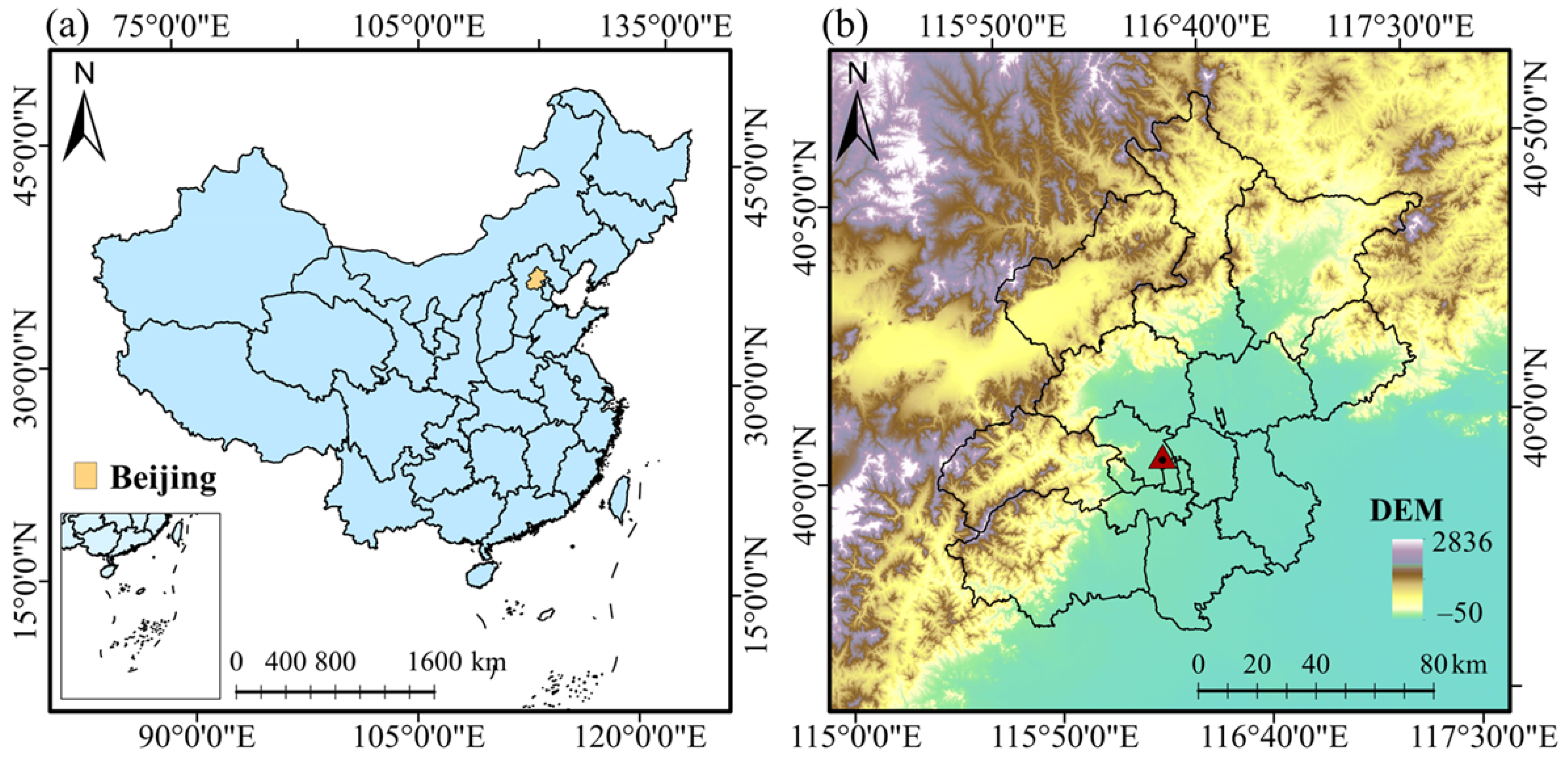
Beijing (Figure 1a), the capital of China, is located at the northwestern margin of the North China Plain [20]. It is characterized by pronounced terrain contrasts, with higher elevations to the northwest and lower elevations toward the southeast (Figure 1b). Beijing spans a total land area of 16,807.8 km² [21], of which roughly 38% is flat and 62% is mountainous [22]. The city experiences a warm temperate semi-humid continental monsoon climate, which is characterized by hot humid summers and cold dry winters [23]. As the second-largest city in the country, the Beijing metropolitan area had a population of 21.89 million in 2021, with 87.5% residing in urban areas [24].

Continuous CDWL observations were conducted from June 2022 to July 2023 at an urban site (39.98°N, 116.34°E) in Haidian District, Beijing. The surrounding area is densely built and urban with pronounced urban boundary-layer characteristics. The lidar was employed on an open platform free of persistent obstructions in the velocity-azimuth display (VAD) scanning sector, ensuring reliable wind-profile retrievals. All heights reported in this study are expressed as height above ground level (AGL). The CDWL system operates at an eye-safe wavelength of 1.5 µm and achieves a maximum detection range of up to 13 km. The wide-band carrier-to-noise ratio (CNR) is used for quality control of raw radial wind speeds [25].

Table 1. Key operating and retrieval-related parameters of the CDWL system.

Parameter	Value
Wavelength	1.5 µm
Pulse energy	150 μJ
Pulse duration	300 ns
Pulse repetition rate	10 kHz
AOM frequency shift	80 MHz
Telescope diameter	70 mm
Sampling frequency	500 MHz
Range-gate length	30/60/150 m
Scan mode	VAD
Elevation angle	60°
Azimuth range (step)	0–360° (5°)
Radial time resolution	1 s
Scan cycle length	~2 min
CNR threshold	−35 dB
Maximum detection range	~13 km

summarizes the key operating parameters of the Doppler lidar system. Detailed information about the validation and application of the lidar system can be found in our previous works [26,27,28,29].

2.2. Lidar Parameter Retrieval Method

A coherent lidar system estimates the radial velocity of aerosol particles illuminated by the lidar pulse as it travels through the atmosphere [30]. To derive the vertical wind profile from these radial velocities, the widely used VAD technique is employed. The core assumption of VAD is horizontal wind homogeneity within the measurement volume during a short scan period (typically under a minute). While complex terrain or strong turbulence coupled with weak winds can challenge this assumption near the surface, the wind field at higher altitudes is generally more uniform. Consequently, the homogeneity assumption remains robust for upper-level retrievals despite the increased scan radius [31].

Before VAD wind retrieval, radial velocity measurements are quality-controlled by a fixed-threshold CNR of −35 dB. Then the filtered sine-wave fitting (FWSF) method is used to retrieve the wind profiles at each height level [25,26,32]. To further guarantee data reliability, the fitting residuals are evaluated using a quality factor (Q-factor); retrievals with a Q-factor below 0.35 are discarded. Finally, the retained wind vectors follow standard meteorological conventions: 0° represents a northerly wind with angles increasing clockwise, and vertical velocity is defined as negative for updrafts and positive for downdrafts.

Turbulence activity can be characterized by several metrics, including vertical velocity variance, spectrum width, turbulent kinetic energy, and the turbulent kinetic energy dissipation rate (TKEDR) [32]. In this study, TKEDR is derived by fitting the azimuth structure function of radial velocity to its theoretical model prediction.

$$TKEDR={\left[{\displaystyle \frac{\overline{D_L\left({\phi }_l\right)}-\overline{D_L\left({\phi }_1\right)}}{A\left(l{\Delta y}_k\right)-A\left({\Delta y}_k\right)}}\right]}^{3/2}$$

Here, the overbar denotes averaging over valid azimuth samples; $D_L\left({\phi }_l\right)$ and $D_L\left({\phi }_1\right)$ are the azimuth structure functions for the l-th and first azimuthal separations, respectively; $A\left(y\right)$ is the theoretical calculation function; ${\Delta y}_k = \Delta \theta R_k cos \phi$ is the transverse separation at range gate k ($\Delta \theta$ in radians), with $l \ge 2$. A 30 min moving average was used in the calculation to ensure statistical stability. Retrievals lacking enough valid azimuthal samples or with unreliable structure-function fits are excluded.

MLH is a turbulence-based boundary-layer metric that describes the height of active vertical turbulent exchange. Following previous approaches [28,33], we determine the MLH from quality-controlled TKEDR profiles, defining it as the height where TKEDR drops below the threshold of 10⁻⁴ m² s⁻³. The applicability of the lidar-derived boundary-layer height product has been evaluated in a previous Beijing study using the same CDWL system, with comparisons and validation against AMDAR and radiosonde observations [34]. Additionally, CNR-based information is retained as an auxiliary tracer to analyze aerosol-layer structures and identify stable or residual layers under weak turbulence conditions.

Building on previous climatology studies of low-level jets (LLJs) in China [35,36,37,38], this study identifies LLJs based on two criteria: the maximum wind speed U_max > 8 m s⁻¹, and the difference in wind speed ΔU = U_max − U_min > 4 m s⁻¹, where U_min is the minimum wind speed above the height of U_max. The jet core height is determined by the height at which U_max occurs. In cases of two-layer LLJs, the lower one is selected. Furthermore, vertical wind shear is defined as the gradient of wind speed and/or direction with respect to altitude. It can be calculated from vertical wind profiles using the vector-based equation [39].

$$\mathrm{V}\mathrm{W}\mathrm{S}\mathrm{H}={\displaystyle \frac{\sqrt{{\left(u_{z_2}-u_{z_1}\right)}^2+{\left(v_{z_2}-v_{z_1}\right)}^2}}{\Delta z}}$$

(1)

where $u$ and $v$ represent the horizontal wind components at two distinct altitude levels, $z_1$ and $z_2$. The numerator denotes the magnitude of the wind vector difference between these levels, which is then divided by the vertical distance $\Delta z=z_2-z_1$. In this study, adjacent vertical range gates were used to determine the shear intensity without any additional vertical smoothing.

3. Results

The results are organized to link wind-field structure, vertical shear, LLJ characteristics, and MLH evolution within a consistent observational framework. We first examine the seasonal vertical distributions of horizontal and vertical winds, and then analyze the diurnal evolution of wind-speed profiles and vertical shear. We next focus on the seasonal characteristics and timing of LLJs, including their occurrence and core-height distributions, before examining the diurnal variation and seasonal contrast of MLH. This organization is intended to highlight the co-variability among wind fields, LLJs, vertical shear, and MLH within the urban boundary layer rather than to present the figures as independent descriptive results.

3.1. Seasonal Vertical Distributions of Horizontal and Vertical Wind

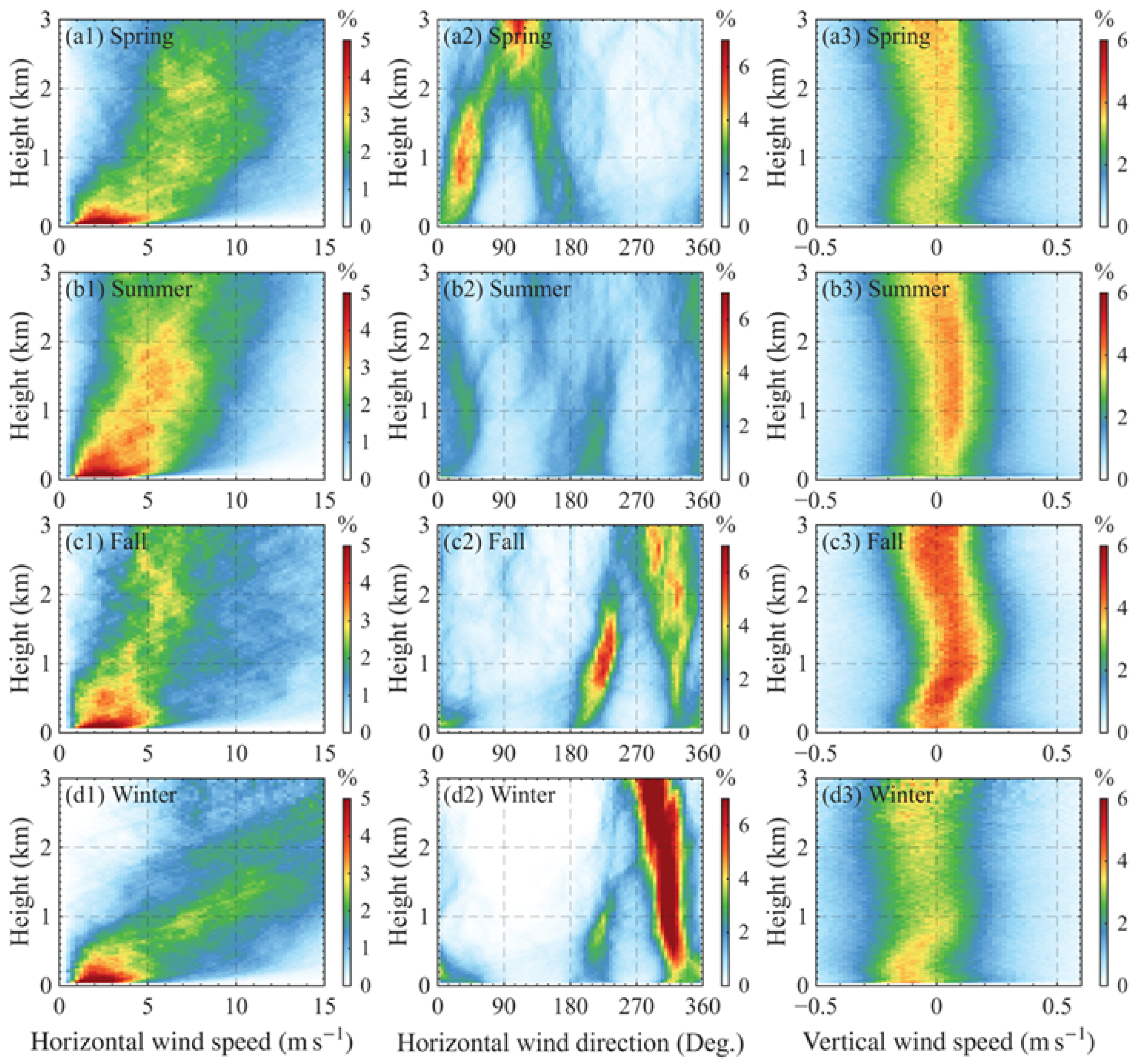
Investigating the characteristics of wind fields at different heights is essential for understanding atmospheric boundary layer physics. We retrieve vertical profiles of wind fields below 3 km and calculate the occurrence frequency at the corresponding height AGL. The left panel of Figure 2 presents the vertical distributions of horizontal wind speed (m s⁻¹) frequency, while the middle panel illustrates the corresponding horizontal wind direction (°) frequency. The vertical wind speed (m s⁻¹) frequency is shown in the right panel. Note that the sum of all frequency values along the x-axis equals 100% at any specific height. For example, a high frequency value of horizontal wind speed indicated by the red color in the figures signifies that the corresponding wind speed is the most prevalent at the specific height.

The overall vertical distribution of horizontal wind speed frequency values (left panel of Figure 2) follows a similar variation, with high frequencies concentrated near the surface and decreasing with height. This can be explained by the fact that horizontal wind speeds increase rapidly with height as surface friction diminishes. Among the seasons, winter experiences the highest wind speeds (>10 m s⁻¹) below 3 km, with the majority of frequency values exceeding 2%. Spring exhibits the second highest horizontal wind speeds, followed by fall and summer. Below 1 km, high frequency values (>3%) are primarily concentrated in the wind speed range between 1 and 5 m s⁻¹ across all seasons. In contrast, high frequency values above 1 km are more dispersed in winter and spring compared to summer and fall. These results suggest that horizontal wind speeds increase the fastest in winter and spring. Compared with our previous lidar study conducted in Hefei [40], Beijing shows relatively higher horizontal wind speed profiles below 3 km throughout the year.

The vertical patterns of horizontal wind direction frequency (middle panel of Figure 2) differ among seasons. In winter, the frequency values (>6%) between 270° and 330° are significantly higher than those in other directional sectors above 0.3 km, suggesting the dominance of northwesterly winds. Below 1.3 km, southwesterly winds (200–240°) also occur prominently, with frequency values exceeding 2%. Similarly, predominant wind directions from the southwest and northwest are observed in fall. However, the highest frequency values (>5%) occur within the 200–240° sector below 2 km, while winds from 270–330° are more frequent (>4%) in the upper levels above 2 km. In spring, the dominant horizontal wind directions are within the 0–60° sector below 2 km. In contrast, the frequency values of horizontal wind direction are concentrated within the 90–120° sector above 2 km. This vertical shift in wind direction is accompanied by stronger horizontal wind speeds, likely associated with the influence of large-scale synoptic systems. In summer, the vertical distribution of horizontal wind direction is the most diverse with the majority of frequency values remaining below 3%. However, relatively high frequency values are observed within the 0–60° and 180–225° sectors below 2 km.

The seasonal frequency distributions of corrected vertical wind speed are shown in the right panel of Figure 2. A small median-based offset correction of +0.063 m s⁻¹ is applied before the frequency-distribution analysis to reduce the weak long-term bias in the VAD-derived vertical velocity below 3 km. Following the sign convention used in previous CDWL studies, negative vertical wind speed indicates upward motion, whereas positive values indicate downward motion. The corrected vertical wind speed is generally concentrated near zero, indicating that the seasonal differences are mainly reflected in the distribution center, width, and vertical structure rather than in persistent strong upward or downward motion. Spring shows a near-zero to weak negative distribution through most of the lower 3 km. Summer is mostly centered near zero, with a slight positive shift at some heights, suggesting weak volume-averaged downward or near-neutral motion rather than enhanced upward motion. Fall displays the broadest and most pronounced distribution, indicating stronger vertical-velocity variability. Winter shows a more evident negative center in the lower layer, corresponding to more frequent weak upward motion under the adopted sign convention. Considering the sensitivity of VAD-derived vertical velocity to scan geometry, weak-signal conditions, and possible aerosol or hydrometeor contamination, these patterns are interpreted cautiously as frequency-distribution characteristics rather than direct evidence of persistent vertical motion.

3.2. Diurnal Evolution of Wind-Speed Profiles and Vertical Shear

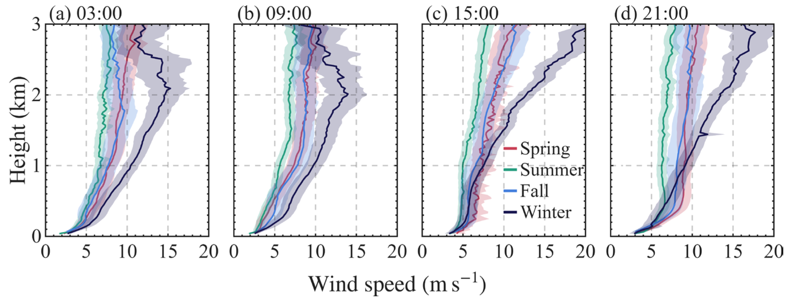
The diurnal evolution of horizontal winds reflects boundary-layer processes and their interaction with the underlying surface. Figure 3 shows the seasonal profiles of wind speed at four representative timestamps in local time (LT) of 03:00, 09:00, 15:00, and 21:00. Among all seasons, the largest wind speed gradients below 1 km are observed at 03:00, followed by 21:00, 09:00, and 15:00 LT. Seasonally, winter exhibits the highest wind speeds across all altitudes and timestamps, particularly above 1 km, where speeds significantly exceed those of the other three seasons. Notably, a significant decrease in wind speed (∆ = −4 m s⁻¹) occurs above 2 km at 03:00 and 09:00 LT during winter. Fall also exhibits a negative or minimal wind speed gradient above 2 km at 03:00, 09:00, and 21:00 LT. At 15:00 LT, seasonal wind speeds increase minimally below 1 km but exhibit the fastest growth above 1 km. Specifically, winter wind speeds at 15:00 LT increase markedly with height, ranging from 4 m s⁻¹ near the surface to 20 m s⁻¹ at 3 km, while other seasons follow a more gradual increasing trend with much lower magnitudes (typically <12 m s⁻¹ at 3 km).

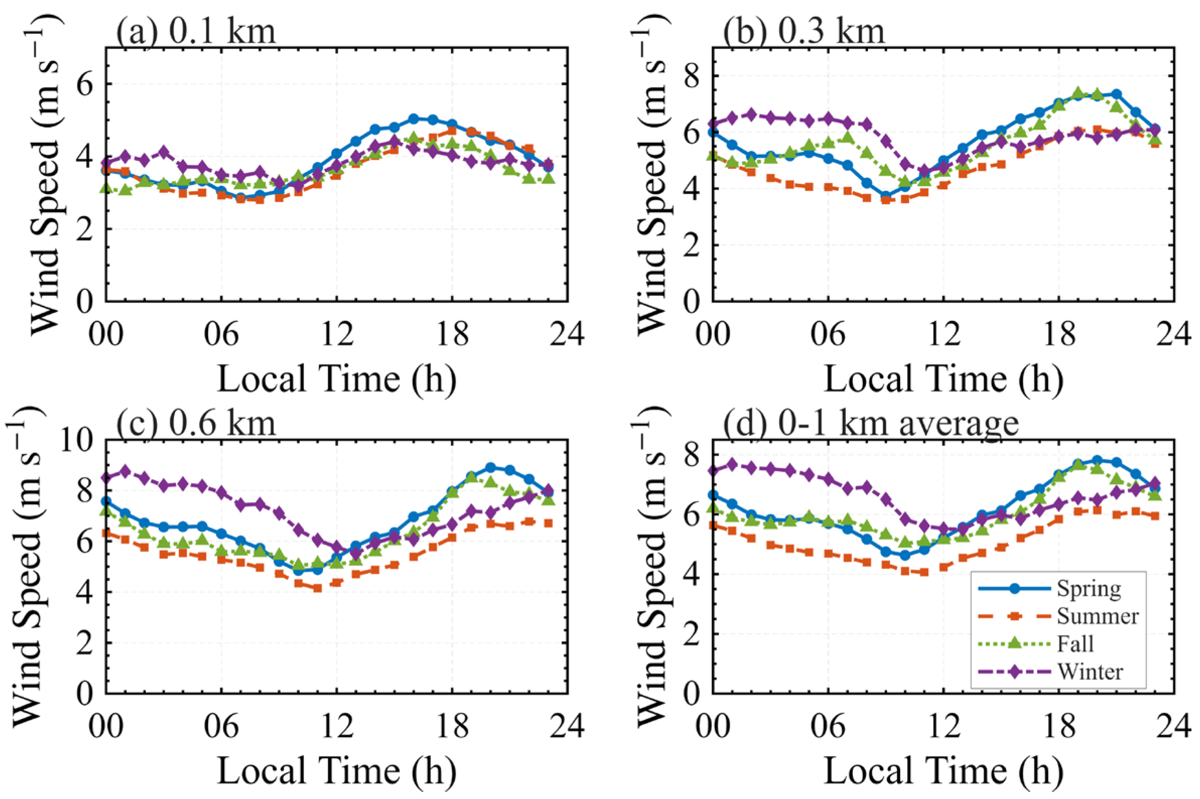
The timing and vertical structure of the diurnal wind speeds differ between the near-surface layer and the air aloft (Figure 4). At 0.1 km, wind speed generally increases after sunrise, peaks in the afternoon, and weakens after sunset (Figure 4a). However, starting from 0.3 km (Figure 4b), a distinct reversal in the diurnal cycle phase is observed across all seasons, with wind speeds strengthening at night and weakening during the morning. At 0.6 km (Figure 4c), this nocturnal enhancement is more pronounced, with winter wind speeds remaining consistently higher than other seasons by approximately 2 m s⁻¹. For the 0–1 km layer-mean wind speed, hourly wind-speed profiles are first calculated at each height level, and then an arithmetic mean is taken over all valid height levels between 0 and 1 km AGL. Because the retrieved wind profiles are on an approximately uniform vertical grid, no additional vertical weighting is applied. Missing values at individual height levels are omitted from the vertical average. The 0–1 km mean wind speed (Figure 4d) exhibits a diurnal pattern similar to those at 0.3 km and 0.6 km, dominated by the nocturnal maximum.

Across all height levels above 0.3 km, the peak speeds generally occur in the early evening (19:00–20:00 LT) in most seasons, except in winter when the maximum appears around 01:00 LT. This nocturnal enhancement becomes more pronounced with height, as supported by the vertical profiles at representative timestamps (Figure 3). Consequently, the largest vertical speed gradients are observed at 21:00 and 03:00 LT rather than at 09:00 and 15:00 LT. This structure is consistent with the establishment of a stable nocturnal boundary layer and decoupling from surface friction, which favors low-level jet formation [40].

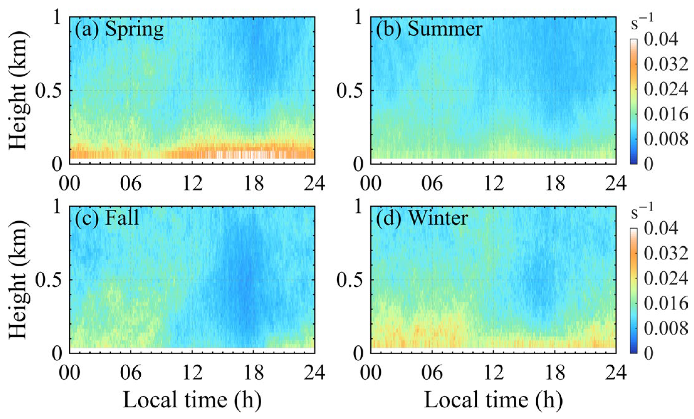
The vertical wind shear derived from CDWL observations exhibits pronounced seasonal contrasts in the intensity, duration, and vertical extent of high-shear regimes (Figure 5). Spring (Figure 5a) is characterized by the most persistent and intense shear environment. High background shear values exceeding 0.016 s⁻¹ are primarily observed below 0.5 km throughout the entire diurnal cycle. The most concentrated high-shear core is found below 0.2 km, where peak values frequently exceed 0.035 s⁻¹ from the afternoon to the early-evening hours. Even during the typical convective window (12:00–16:00 LT), the shear intensity in the lower layers remains significantly elevated compared to other seasons. In summer, high-shear occurrences are the most fragmented and vertically restricted. The nocturnal high-shear layer (>0.024 s⁻¹) is relatively thin, seldom extending above 0.2 km, and often appears discontinuous in time.

Fall and winter seasons show more defined transitions between nocturnal and daytime regimes of vertical shear. High-shear values in fall are strictly confined to the nocturnal and early-morning periods. Following a sharp transition after 20:00 LT, a high-shear layer gradually develops near the surface. While the intensity can reach 0.02 s⁻¹ in the lowermost levels, the regime is characterized by a rapid collapse after 09:00 LT, showing a very clear temporal boundary. Winter exhibits a unique high-shear structure marked by significant vertical stretching and prolonged duration. High-shear values exceeding 0.016 s⁻¹ persist below 0.5 km throughout the day, similar to spring. However, the nocturnal strong shear zone (>0.024 s⁻¹) in winter is markedly thicker, frequently extending to altitudes of 0.3–0.4 km. This high-shear state also shows the greatest persistence, remaining intact until ~10:00 LT before any noticeable reduction occurs.

To quantify the seasonal shear regimes shown in Figure 5,

Table 2. Seasonal statistics of vertical wind shear (VWS, s⁻¹) below 0.5 km and 1.0 km AGL. Statistics are calculated from the seasonal median VWS fields. P95 denotes the 95th percentile of VWS and is used to represent the upper-tail shear intensity. Daytime is defined as 08:00–18:00 LT, and nighttime is defined as 20:00–08:00 LT. Strong-shear fractions indicate the percentage of samples exceeding 0.016 s⁻¹ and 0.024 s⁻¹.

Season	Layer	Mean (s−1)	P95 (s−1)	Nocturnal Mean (s−1)	Daytime Mean (s−1)	Fraction > 0.016 (%)	Fraction > 0.024 (%)
Spring	0–0.5 km	0.0184	0.0323	0.0186	0.0182	54.1	17
	0–1.0 km	0.0148	0.0274	0.0151	0.0147	26.4	8.1
Summer	0–0.5 km	0.0141	0.0189	0.0145	0.0139	23.9	0.0
	0–1.0 km	0.0122	0.0178	0.0126	0.0121	11.3	0.0
Fall	0–0.5 km	0.013	0.0191	0.015	0.0113	24	0.0
	0–1.0 km	0.0122	0.0179	0.0133	0.0113	11.6	0.0
Winter	0–0.5 km	0.017	0.0244	0.0186	0.0155	55	6.3
	0–1.0 km	0.0146	0.0230	0.0154	0.0140	27.1	3.0

summarizes VWS statistics below 0.5 km and 1.0 km AGL, including the mean value, P95 value, and strong-shear fractions. The statistics confirm that spring and winter exhibit stronger low-level shear than summer and fall. Below 0.5 km, the mean VWS reaches 0.0184 s⁻¹ in spring and 0.0170 s⁻¹ in winter, compared with 0.0141 s⁻¹ in summer and 0.0130 s⁻¹ in fall. Strong-shear fractions exceeding 0.016 s⁻¹ are also highest in spring and winter, reaching 54.1% and 55.0%, respectively. More intense shear exceeding 0.024 s⁻¹ occurs mainly in spring, whereas such values are nearly absent in summer and fall.

3.3. Seasonal Characteristics and Timing of Low-Level Jets

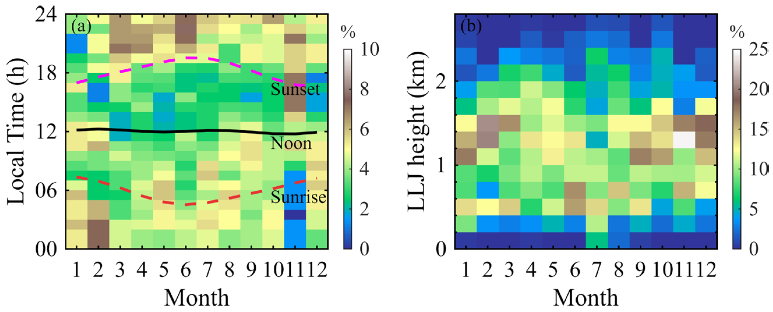
LLJs are commonly defined as fast-moving wind streams with the maximum wind speed and vertical wind shear in the lower troposphere [1,33]. The frequency of LLJ occurrence (%) is defined as the proportion of valid observational days in a given month on which at least one LLJ is detected below 3 km AGL relative to the total number of valid observational days in that month. To characterize their seasonal and diurnal behavior at the Beijing site, the month–hour (Figure 6a) and month–height distributions of LLJ frequency (Figure 6b), along with seasonal wind-rose diagrams at the jet-nose height (Figure 7), are presented. The month–time and month–height distributions in Figure 6 are normalized within each month to highlight the preferred occurrence time and core-height distribution. These figures highlight key aspects of LLJ variability, including the timing of maximum occurrence, preferred core height, and wind direction and speed.

LLJs exhibit pronounced diurnal asymmetry and seasonal shifts in both occurrence and core height. LLJs occur primarily between 20:00 and 08:00 LT, with minimal daytime activity (11:00–17:00 LT) due to convective mixing disrupting low-level shear. Seasonally, spring features concentrated nocturnal activity, peaking in March and April during late evening and early night, with May showing a strong late-night maximum (~22:00 LT) and a secondary early-morning peak. Jet-nose heights gradually range from 1.6 km in March to 1.2–1.4 km in May, with April representing the most vertically dispersed month, with nearly uniform frequencies across 0.8–1.8 km (7–11%), indicating a more complex vertical distribution of LLJ occurrence during spring. Summer LLJs are confined to late evening through early morning (20:00–04:00 LT), with August peaking near sunrise (~05:00 LT). A sharp transition in jet-nose height occurs between May and June, with the primary core shifting downward from 1.2–1.4 km to 0.6–0.8 km and increased contributions from 0.4–0.6 km.

Fall exhibits more persistent nocturnal and early-morning jets, with November displaying an unusually early and extended high-frequency period spanning 14:00–21:00 LT (>7%), modal heights rising to 1.2 km in September–October, and a pronounced maximum near 1.4 km in November (~24.6%), the most vertically concentrated core of the year, suggesting more stable autumn boundary-layer conditions. Winter (December–February) LLJs peak during early-morning hours (01:00–05:00 LT), with December showing a broader morning maximum and February exhibiting the strongest peak; jet noses are the highest of the year, typically between 1.2 and 1.6 km, peaking at 1.6 km in December and February, consistent with cold-season stable stratification. Together, these patterns reveal a shift from strong vertical dispersion in spring (April) to enhanced concentration in late autumn (November) and a lower jet-core distribution in summer, suggesting seasonal differences in the thermal and dynamical conditions associated with LLJ occurrence.

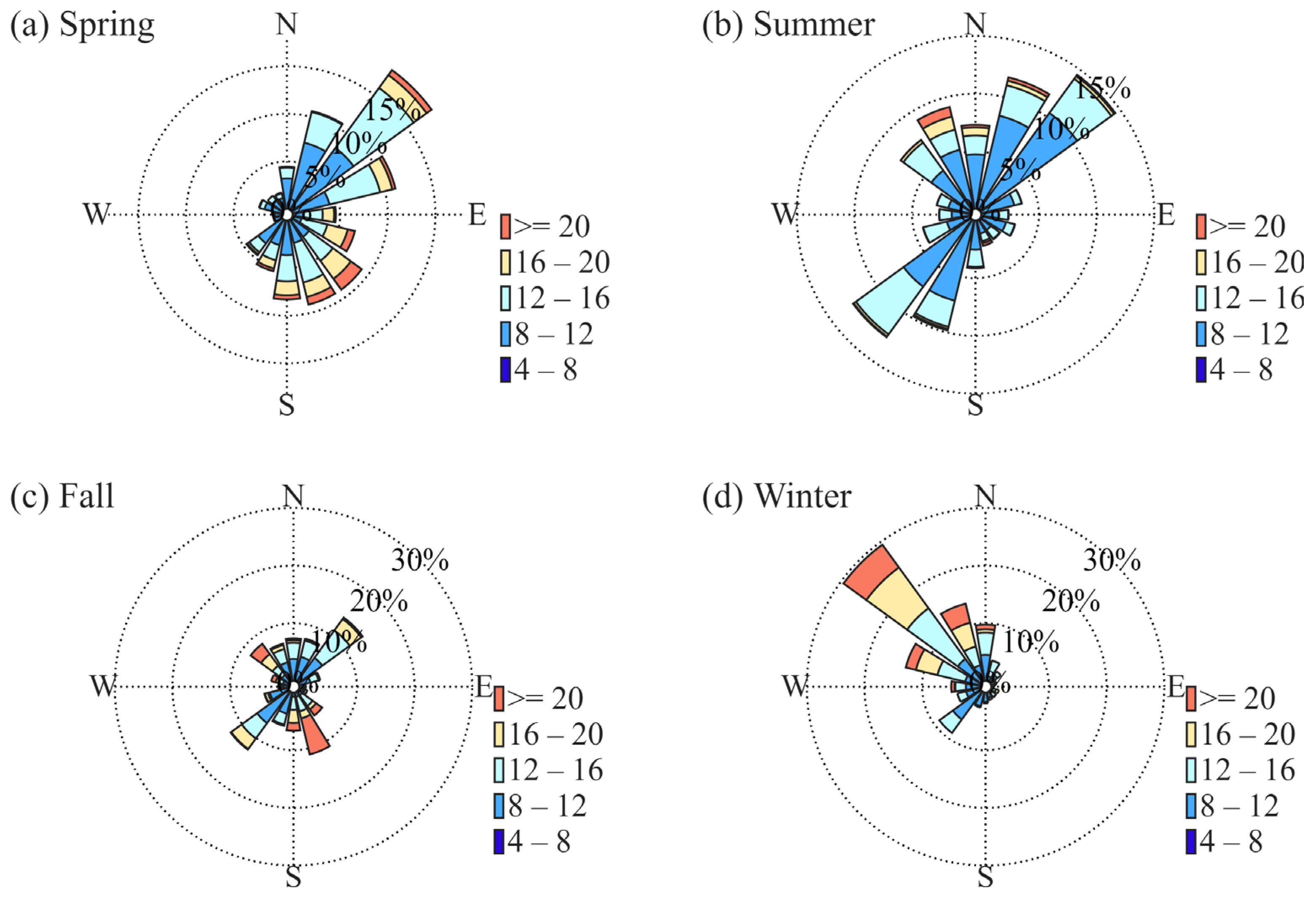
Across seasons, winds at the jet-nose heights are frequently from the southwest but differ systematically in directional concentration and speed distribution. In Figure 7a, LLJs in spring are dominated by the southwest sector (210–240°, 14.8%), with a secondary maximum in the northeast sector (30–60°, 13.3%). The occurrence of maximum jet speed is primarily distributed within the broader 8–16 m s⁻¹ interval (73.9%), with the 10–12 m s⁻¹ and 12–14 m s⁻¹ categories contributing most strongly. Summer exhibits the strongest directional concentration among all seasons, with the southwest sector (210–240°) overwhelmingly dominant (20.8%) and prevailing across most wind-speed categories (Figure 7b). The majority of occurrences fall within the 8–14 m s⁻¹ bin (85.8%), with a pronounced maximum in the 8–10 m s⁻¹ bin (41.2%). Fall (Figure 7c) also shows a distinct southwest peak (25.1%) and is associated with a wide range of wind speeds (8–14 m s⁻¹, 75.2%). Secondary contributions are evident in the northeast (30–60°, 17.6%) and northwest (315–340°, 10.7%) sectors. The wind rose at the jet-nose height in winter (Figure 7d) exhibits a broad directional distribution, with the most frequent occurrence in the southwest sector (210–240°, 15.9%) and a secondary contribution from the northwest sector (300–330°, 14.4%). The jet-nose flow is concentrated mainly in the 8–16 m s⁻¹ range (78.9%), with appreciable contributions also from the 8–10 m s⁻¹ (23.5%) and the 10–12 m s⁻¹ (23.6%) bins.

To provide a quantitative summary of the monthly LLJ characteristics,

Table 3. Monthly statistics of LLJ occurrence days, jet-core height, and jet speed. LLJ occurrence days are defined as days on which at least one valid LLJ is detected below 3 km AGL. Jet-core height and jet-speed statistics are calculated from all valid LLJ profiles below 3 km AGL in each month. The LLJ-day ratio is defined as the number of LLJ occurrence days divided by the number of valid observation days in each calendar month.

Month	LLJ-Day Ratio (%)	Mean Core Height (km)	Median Core Height (km)	Mean Jet Speed (m s−1)	Median Jet Speed (m s−1)
1	90.3	1.14	1.18	14.0	12.9
2	46.2	1.48	1.49	13.0	12.3
3	94.1	1.21	1.18	14.4	13.4
4	96.7	1.39	1.36	13.5	12.8
5	83.3	1.27	1.26	11.5	10.7
6	77.8	1.16	1.07	12.4	11.9
7	88.9	1.26	1.08	11.4	10.7
8	93.1	1.37	1.35	12.2	11.0
9	83.3	1.07	1.07	12.0	11.3
10	96.0	1.44	1.41	16.3	15.5
11	100.0	1.25	1.31	16.0	15.2
12	86.7	1.25	1.31	14.4	13.7

lists the number of valid observational days, LLJ occurrence days, jet-core height statistics, and jet-speed statistics for each month. Here, LLJ days indicate valid observational days with at least one LLJ occurrence below 3 km AGL. Jet-core height and jet-speed statistics are calculated from all valid LLJ profiles below 3 km AGL in each month. The monthly statistics complement the month–time and month–height frequency distributions shown in Figure 6 and the seasonal wind-direction characteristics shown in Figure 7. The strongest monthly mean jet speeds occur in the cold and transition seasons, with values exceeding 14 m s⁻¹ in January, March, October, November, and December. In contrast, weaker monthly mean jet speeds are found in late spring and summer, especially in May and July, when the mean jet speed remains close to 11–12 m s⁻¹. Monthly mean and median core heights are generally located between about 1.1 and 1.5 km, indicating that the monthly averaged jet-core layer is mainly concentrated in the lower troposphere.

3.4. Diurnal Variation and Seasonal Contrast of the Mixing-Layer Height

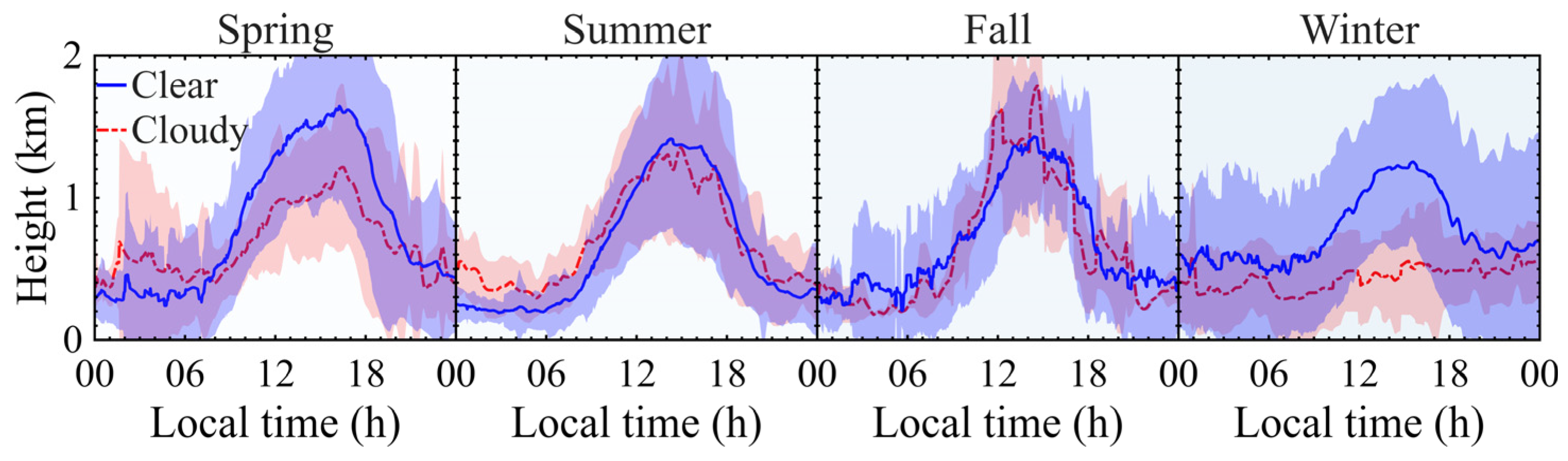
The seasonal mixing-layer height (MLH, Figure 8) is derived from turbulence-related parameters (i.e., TKEDR) based on CDWL observations. Clear-sky and cloudy days are classified following the weather-type definition used in our previous CDWL study [40]. Clear-sky days are defined as days with cloud occurrence lasting less than 2 h, whereas cloudy days are defined as days with cloud occurrence exceeding 8 h. Rainy days, defined as days with rainfall persisting for more than 2 h, are excluded from the clear/cloudy MLH comparison. Partly cloudy days, with cloud occurrence lasting between 2 and 8 h, are not included in Figure 8. Thus, the clear/cloudy comparison represents a broad lidar-observed weather-type contrast rather than a cloud-type-specific analysis. Because MLH is most physically relevant to the daytime convective mixed layer, the following analysis focuses primarily on daytime MLH growth, peak development, and decay. Nighttime and early-morning values are shown in Figure 8 to maintain the continuity of the diurnal cycle, but they are not interpreted as fully developed daytime mixed-layer depths. Under clear-sky conditions at the urban Beijing site, the MLH is significantly higher than under cloudy conditions across most seasons, with the exception of fall. Spring exhibits the deepest MLH among all seasons, with the growth typically initiating after 08:00 LT and reaching clear-sky peaks frequently exceeding 1.5 km between 14:00 and 17:00 LT. In contrast, the summer MLH is generally shallower, with growth beginning earlier around 07:00 LT but peaking at a lower range (typically remaining below 1.4 km) near 15:00 LT, despite stronger insolation and a higher frequency of clear-sky days. In fall, the MLH exhibits a rapid growth rate during the afternoon under clear-sky conditions, reaching peaks (~1.3 km) that are comparable to those in summer. Notably, autumn is the only season where the mean MLH under cloudy skies occasionally matches or exceeds the clear-sky levels during the late afternoon, suggesting that the cloudy-day MLH response in fall may be modulated by additional meteorological factors rather than cloudiness alone. Winter displays the lowest and most suppressed MLH, with clear-sky peaks typically constrained below 1.2 km. The growth of the winter MLH is markedly delayed, only showing a significant rise after 10:00 LT, which coincides with the dissipation of the deep nocturnal wind shear layer (Figure 5d).

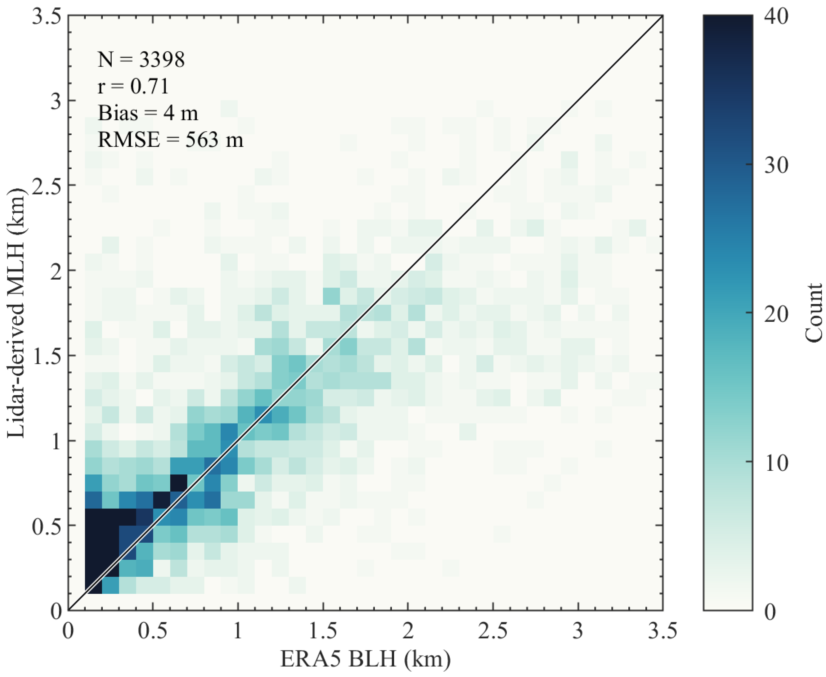
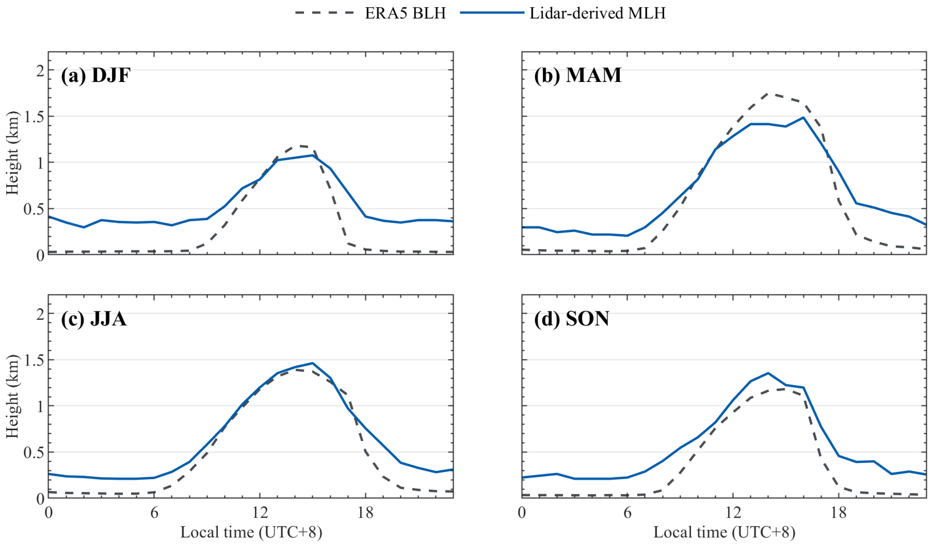
As an additional consistency check, the lidar-derived MLH is compared with ERA5 boundary-layer height (BLH) using hourly matched data. ERA5 BLH is not treated as an observational ground truth because it differs from the lidar-derived MLH in definition, spatial representativeness, and model parameterization. Nevertheless, the density scatterplot shows that the two products exhibit a broadly positive correspondence in daytime boundary-layer depth (Figure A1). Their seasonal diurnal composites also show similar daytime growth and seasonal evolution, although differences remain in magnitude and timing (Figure A2). Therefore, the ERA5 comparison is used here to support the interpretation of relative seasonal and diurnal MLH variability rather than to provide a direct validation of the absolute MLH retrieval accuracy.

The fifth-generation ECMWF reanalysis (ERA5) dataset, providing global climate and weather data from January 1940 to present, is used to calculate surface sensible and latent heat fluxes. To better represent the surface-energy forcing relevant to daytime MLH development, SHF, LHF, and the Bowen ratio are calculated using daytime values from 08:00 to 18:00 LT.

Table 4. Seasonal daytime surface-flux statistics derived from ERA5 hourly single-level data at the grid cell corresponding to the Beijing observational site. The table includes clear-sky days, daytime-mean sensible heat flux (SHF), daytime-mean latent heat flux (LHF), daytime-mean Bowen ratio, and sample size. Samples indicate the number of hourly ERA5 records used for the daytime statistics. Daytime is defined as 08:00–18:00 LT.

Season	Clear-Sky Days	SHF (W m−2)	LHF (W m−2)	Bowen Ratio	Samples
Spring	41	139.8	95.1	1.47	920
Summer	64	96.2	187.8	0.51	1530
Fall	47	89.5	76.5	1.17	910
Winter	58	66.4	23.4	2.84	900

summarizes the seasonal daytime-mean SHF, daytime-mean LHF, and daytime-mean Bowen ratio extracted from the ERA5 grid cell corresponding to the Beijing observational site. Spring is characterized by a higher SHF (139.8 W m⁻²) and a Bowen ratio of 1.47, which is consistent with stronger sensible-heat-driven mixing. Conversely, summer is dominated by daytime LHF (187.8 W m⁻²) with a lower Bowen ratio of 0.51. Beyond thermal forcing, the diurnal variation in seasonal vertical wind shear reveals that the background and near-surface wind shear in spring remain higher than those in summer throughout most of the day, providing conditions favorable for persistent mechanical turbulent mixing. These results suggest that MLH development is associated not only with local solar heating but also with seasonal differences in surface-energy partitioning and low-level wind shear. In summer, the humid atmosphere partitions more energy into latent heat rather than sensible heat, limiting the surface-driven turbulent mixing and MLH growth. In contrast, the high wind speeds observed in spring (peaking at >15 m s⁻¹ above 1 km, Figure 3) and enhanced vertical shear may provide stronger mechanical mixing, which together with higher daytime sensible heat flux may favor the development of a deeper MLH.

4. Discussion

The year-long lidar observations indicate pronounced seasonal and diurnal variability of the lower atmosphere at the urban Beijing site, which is likely influenced by the combined action of large-scale circulation, topographic modulation, and urban boundary-layer processes. The stronger winds observed in winter and spring are consistent with the stronger cold-season background forcing over northern China, whereas the weaker and more directionally dispersed summer flow is consistent with the seasonal influence of moist monsoonal conditions. During summer, the monsoonal background may also enhance atmospheric moisture and latent heat partitioning, which is consistent with the relatively limited daytime MLH growth despite stronger solar heating. This broader interpretation is supported by recent observations across China showing that upper-air wind speed over northern China tends to strengthen in winter and that wind variability must be interpreted from combined vertical, regional, and seasonal perspectives [41]. In Beijing, this seasonal forcing is further modified by the city’s position between the North China Plain and the surrounding mountains, which favors the interaction of regional airflow with terrain-induced circulations. This interpretation is broadly consistent with recent work showing that LLJs in the Beijing area are strongly affected by the Taihang and Yanshan Mountains and that their dominant directions are mainly from the southwest and northwest [42]. Given the directional preference shown in the wind-rose analysis, a future sector-based analysis would be useful for separating terrain-modulated flows from other synoptic and urban influences. The present results therefore suggest that the wind field observed at this urban Beijing site cannot be interpreted as a simple response to surface heating alone, but rather is likely affected by the large-scale circulation and terrain-modulated boundary-layer processes.

At the diurnal scale, wind fields, low-level jets, vertical shear, and MLH show coherent diurnal variations and may represent related aspects of boundary-layer adjustment. The nocturnal strengthening of winds above the near-surface layer, together with enhanced vertical shear and frequent LLJ occurrence, is consistent with nighttime decoupling and the redistribution of momentum aloft under stable conditions. Earlier climatological analyses in Beijing likewise showed that LLJ occurrence is closely tied to favorable synoptic conditions, confirming that such jets are a recurrent feature of the regional boundary layer rather than isolated events [37]. After sunrise, renewed turbulent mixing may redistribute momentum vertically and weaken nocturnal jet structures, which is consistent with daytime boundary-layer growth. In this context, the seasonal contrast in MLH is particularly revealing. Previous observations over Beijing reported a clear seasonal cycle in MLH, with deeper development in spring and summer, and lower values in winter [43,44], while a recent one-year urban Beijing study showed that boundary-layer stability is jointly modulated by radiation, wind, and turbulence [45]. The present results are broadly consistent with those findings, but further suggest that MLH at this urban Beijing site can be discussed in the context of nocturnal wind structure and LLJ-related shear, rather than as an isolated response to daytime heating alone. In particular, the deeper spring MLH and the comparatively shallower summer MLH are consistent with the combined influence of sensible heating, mechanical mixing, and the inherited nocturnal dynamical structure on daytime boundary-layer development. This interpretation is also consistent with [46], who emphasized the combined roles of thermal and dynamical forcing in boundary-layer evolution over urban Beijing.

Compared with previous studies using different observational platforms or selected case analyses, the present year-long CDWL dataset provides a consistent height-resolved basis for examining wind profiles, LLJs, vertical shear, and lidar-derived MLH at the same urban site. The present interpretation is supported by several observational considerations. First, the year-long continuous lidar observations provide robust coverage of both seasonal and diurnal variability. Second, previous validation and application studies have demonstrated the reliability of the CDWL observations and associated retrievals in cities including Beijing [26,27,28,47]. Third, multiple boundary-layer diagnostics, including wind fields, LLJs, vertical shear, and MLH, show internally consistent behavior, lending support to the present observational interpretation. Nevertheless, several limitations should be acknowledged. First, the analysis is based on a single urban lidar site and therefore cannot fully resolve the spatial heterogeneity of boundary-layer structure across the broader Beijing metropolitan region. Second, the retrieval of MLH and the identification of LLJs depend on method-specific parameters and threshold criteria, which may influence the exact frequencies, heights, and intensities reported here. In addition, collocated ceilometer, micropulse lidar, radiosonde, or tower-based turbulence observations covering the full study period are not available; therefore, a point-by-point validation of the lidar-derived MLH using bias, RMSE, and correlation statistics cannot be performed in this study. Although an ERA5-based consistency check has been included, ERA5 BLH is not used as an observational ground truth because of differences in definition, spatial representativeness, and model parameterization. The MLH results are therefore interpreted mainly in terms of relative seasonal and diurnal variability rather than as an independent validation of the retrieval algorithm. Third, although the year-long dataset provides robust observational evidence of seasonal and diurnal variability, the present study remains primarily observational and does not include an explicit weather-type or circulation-pattern classification, and therefore cannot fully distinguish the relative contributions of synoptic forcing, terrain effects, and urban surface processes. Therefore, the mechanism-related discussion should be regarded as a physically plausible interpretation based on the observed lidar statistics and previous studies, rather than as a direct attribution analysis. Future work combining multi-site observations, radiosonde profiles, and high-resolution numerical simulations would help to better constrain the mechanisms underlying the seasonal and diurnal boundary-layer variability over Beijing.

5. Conclusions

This study characterizes the seasonal and diurnal variability of wind fields, low-level jets (LLJs), and mixing-layer height (MLH) at an urban site in Beijing based on one year of Doppler wind lidar observations. The results show pronounced seasonal contrasts in the lower-atmospheric wind structure, with generally stronger horizontal winds in winter and spring and weaker, more directionally dispersed flow in summer. A distinct diurnal phase reversal in wind speed is identified near 0.3 km, where nocturnal enhancement aloft contrasts with daytime intensification near the surface. The corrected vertical-velocity distributions also show seasonally varying frequency structures but are interpreted cautiously because of the higher uncertainty associated with VAD-derived vertical velocity. LLJs occur predominantly at night and exhibit clear seasonal differences in occurrence time and jet-core height, with the jet core generally located at 1.2–1.6 km in winter but descending to about 0.6–0.8 km in summer. Monthly statistics further show stronger jet speeds in the cold and transition seasons, with mean values exceeding 14 m s⁻¹ in January, March, October, November, and December. Vertical shear is stronger and more persistent in spring and winter than in summer and fall, especially below 0.5 km AGL. MLH also shows marked seasonal differences, with the deepest development in spring and the shallowest and most delayed growth in winter, whereas the comparatively limited summer growth is consistent with stronger latent heat partitioning.

Overall, these results indicate that wind fields, LLJs, vertical shear, and MLH at this urban Beijing site exhibit coherent seasonal and diurnal covariations, although their direct causal relationships require further process-oriented analysis. The present study provides a year-long observational basis for understanding the seasonal and diurnal variability of the lower atmosphere at the urban Beijing site and for evaluating urban ABL parameterizations using continuous Doppler wind lidar observations. Future work should combine multi-site observations, radiosonde profiles, weather-type classification, and high-resolution numerical simulations to better quantify the respective roles of synoptic forcing, terrain effects, and urban surface processes.

References

1. Stull, R.B. (Ed.) An Introduction to Boundary Layer Meteorology; Kluwer Academic Publishers: Dordrecht, The Netherlands, 1988. [Google Scholar]
2. Mahrt, L. Stratified Atmospheric Boundary Layers. Bound. Layer Meteorol. 1999, 90, 375–396. [Google Scholar] [CrossRef] [Scilit]
3. Mehta, S.K.; Ratnam, M.V.; Sunilkumar, S.V.; Rao, D.N.; Krishna Murthy, B.V. Diurnal Variability of the Atmospheric Boundary Layer Height over a Tropical Station in the Indian Monsoon Region. Atmos. Chem. Phys. 2017, 17, 531–549. [Google Scholar] [CrossRef] [Scilit]
4. Li, Z.; Guo, J.; Ding, A.; Liao, H.; Liu, J.; Sun, Y.; Wang, T.; Xue, H.; Zhang, H.; Zhu, B. Aerosol and Boundary-Layer Interactions and Impact on Air Quality. Natl. Sci. Rev. 2017, 4, 810–833. [Google Scholar] [CrossRef] [Scilit]
5. Wang, M.; Wei, T.; Lolli, S.; Wu, K.; Wang, Y.; Hu, H.; Yuan, J.; Tang, D.; Xia, H. A Long-Term Doppler Wind LiDAR Study of Heavy Pollution Episodes in Western Yangtze River Delta Region, China. Atmos. Res. 2024, 310, 107616. [Google Scholar] [CrossRef] [Scilit]
6. Banakh, V.A.; Smalikho, I.N.; Falits, A.V. Estimation of the Turbulence Energy Dissipation Rate in the Atmospheric Boundary Layer from Measurements of the Radial Wind Velocity by Micropulse Coherent Doppler Lidar. Opt. Express 2017, 25, 22679. [Google Scholar] [CrossRef] [Scilit] [PubMed]
7. Boventer, J.; Bramati, M.; Savvakis, V.; Beyrich, F.; Kayser, M.; Platis, A.; Bange, J. Validation of Doppler Wind LiDAR Measurements with an Uncrewed Aerial System (UAS) in the Daytime Atmospheric Boundary Layer. J. Atmos. Ocean. Technol. 2024, 41, 705–723. [Google Scholar] [CrossRef] [Scilit]
8. Zhang, L.; Xin, J.; Yin, Y.; Liu, R.; Tian, Y.; Lin, Z.; Zhou, X.; Ren, Y.; Zhang, X.; Ma, Y.; et al. Study of Boundary Layer Parameterization Simulation Uncertainties of Sand-Dust Storm Windfield Using High-Resolution Three-Dimensional Doppler Wind Lidar Data. Atmos. Res. 2024, 306, 107456. [Google Scholar] [CrossRef] [Scilit]
9. He, Y.; Ren, C.; Mak, H.W.L.; Lin, C.; Wang, Z.; Fung, J.C.H.; Li, Y.; Lau, A.K.H.; Ng, E. Investigations of High-Density Urban Boundary Layer under Summer Prevailing Wind Conditions with Doppler LiDAR: A Case Study in Hong Kong. Urban Clim. 2021, 38, 100884. [Google Scholar] [CrossRef] [Scilit]
10. Jin, X.; Song, X.; Yang, Y.; Wang, M.; Shao, S.; Zheng, H. Estimation of Turbulence Parameters in the Atmospheric Boundary Layer of the Bohai Sea, China, by Coherent Doppler Lidar and Mesoscale Model. Opt. Express 2022, 30, 13263. [Google Scholar] [CrossRef] [Scilit] [PubMed]
11. Li, N.; Dyer-Hawes, Q.; Romanic, D.; Burlando, M. Investigation of Coastal Winds and Turbulence Characteristics Using Doppler Lidar. J. Geophys. Res. Atmos. 2024, 129, e2024JD041429. [Google Scholar] [CrossRef] [Scilit]
12. Ortiz-Amezcua, P.; Andújar-Maqueda, J.; Manninen, A.J.; Pentikäinen, P.; O’Connor, E.J.; Stachlewska, I.S.; De Arruda Moreira, G.; Benavent-Oltra, J.A.; Casquero-Vera, J.A.; Poczta, P.; et al. Dynamics of the Atmospheric Boundary Layer over Two Middle-Latitude Rural Sites with Doppler Lidar. Atmos. Res. 2022, 280, 106434. [Google Scholar] [CrossRef] [Scilit]
13. Ratynski, M.; Khaykin, S.; Hauchecorne, A.; Wing, R.; Cammas, J.-P.; Hello, Y.; Keckhut, P. Validation of Aeolus Wind Profiles Using Ground-Based Lidar and Radiosonde Observations at Réunion Island and the Observatoire de Haute-Provence. Atmos. Meas. Tech. 2023, 16, 997–1016. [Google Scholar] [CrossRef] [Scilit]
14. Wolz, K.; Holst, C.; Beyrich, F.; Paeschke, E.; Mauder, M. Verifying Triple and Single Doppler Lidar Wind Measurements with Sonic Anemometer Data Based on a New Filter Strategy for Virtual Tower Measurements. EGUsphere 2023. [Google Scholar] [CrossRef] [Scilit]
15. Sun, Z.; Zhao, X.; Li, Z.; Tang, G.; Miao, S. Boundary Layer Structure Characteristics under Objective Classification of Persistent Pollution Weather Types in the Beijing Area. Atmos. Chem. Phys. 2021, 21, 8863–8882. [Google Scholar] [CrossRef] [Scilit]
16. Huang, M.; Gao, Z.; Miao, S.; Chen, F.; LeMone, M.A.; Li, J.; Hu, F.; Wang, L. Estimate of Boundary-Layer Depth over Beijing, China, Using Doppler Lidar Data during SURF-2015. Bound. Layer Meteorol. 2017, 162, 503–522. [Google Scholar] [CrossRef] [Scilit]
17. Tang, N.; Guo, J.; Chen, J.; Li, Z.; Guo, X.; Sun, Y.; Xu, H.; Zhang, Z.; Li, N.; Zeng, L.; et al. Anticyclone Driven Heat Waves Intensify Beijing’s Urban Boundary-Layer Turbulence. Geophys. Res. Lett. 2025, 52, e2025GL115800. [Google Scholar] [CrossRef] [Scilit]
18. Zhao, D.; Xu, H.; Li, Y.; Yu, Y.; Duan, Y.; Xu, X.; Chen, L. Locally Opposite Responses of the 2023 Beijing–Tianjin–Hebei Extreme Rainfall Event to Global Anthropogenic Warming. npj Clim. Atmos. Sci. 2024, 7, 38. [Google Scholar] [CrossRef] [Scilit]
19. Zhu, T.; Zhou, Y.; Yang, J.; Vitart, F.; Bao, Q. Severe Extreme Cold Event in Beijing-tianjin-hebei Region Tied to Mid-high-latitude Intraseasonal Waves. Geophys. Res. Lett. 2025, 52, e2024GL113745. [Google Scholar] [CrossRef] [Scilit]
20. Sun, J.; Li, G.X.; Jayasinghe, R.; Sadler, R.; Shaw, G.; Pan, X.C. Time Course of Apparent Temperature Effects on Cardiovascular Mortality: A Comparative Study of Beijing, China and Brisbane, Australia. Public Health Res. 2012, 2, 43–48. [Google Scholar] [CrossRef] [Scilit]
21. Tian, Y.; Liu, F.; Jim, C.Y.; Wang, T.; Liu, X.; Luan, J.; Yan, M. Strengths and Gaps of Climate Change Perceptions in the Beijing Metropolis. Clim. Serv. 2023, 30, 100350. [Google Scholar] [CrossRef] [Scilit]
22. Song, X.; Zhang, J.; AghaKouchak, A.; Roy, S.S.; Xuan, Y.; Wang, G.; He, R.; Wang, X.; Liu, C. Rapid Urbanization and Changes in Spatiotemporal Characteristics of Precipitation in Beijing Metropolitan Area. J. Geophys. Res. Atmos. 2014, 119, 11250–11271. [Google Scholar] [CrossRef] [Scilit]
23. Liu, J.; Schlünzen, K.H.; Frisius, T.; Tian, Z. Effects of Urbanization on Precipitation in Beijing. Phys. Chem. Earth Parts A/B/C 2021, 122, 103005. [Google Scholar] [CrossRef] [Scilit]
24. Han, L.; Qin, T.; Sun, Z.; Ren, H.; Zhao, N.; An, X.; Wang, Z. Influence of Urbanization on the Spatial Distribution of Associations between Air Pollution and Mortality in Beijing, China. Geohealth 2023, 7, e2022GH000749. [Google Scholar] [CrossRef] [Scilit] [PubMed]
25. Smalikho, I. Techniques of Wind Vector Estimation from Data Measured with a Scanning Coherent Doppler Lidar. J. Atmos. Ocean. Technol. 2003, 20, 276–291. [Google Scholar] [CrossRef] [Scilit]
26. Wei, T.; Xia, H.; Wu, Y.; Yuan, J.; Wang, C.; Dou, X. Inversion Probability Enhancement of All-Fiber CDWL by Noise Modeling and Robust Fitting. Opt. Express 2020, 28, 29662–29675. [Google Scholar] [CrossRef] [Scilit] [PubMed]
27. Wei, T.; Xia, H.; Yue, B.; Wu, Y.; Liu, Q. Remote Sensing of Raindrop Size Distribution Using the Coherent Doppler Lidar. Opt. Express 2021, 29, 17246. [Google Scholar] [CrossRef] [Scilit] [PubMed]
28. Wang, L.; Qiang, W.; Xia, H.; Wei, T.; Yuan, J.; Jiang, P. Robust Solution for Boundary Layer Height Detections with Coherent Doppler Wind Lidar. Adv. Atmos. Sci. 2021, 38, 1920–1928. [Google Scholar] [CrossRef] [Scilit]
29. Wei, T.; Wang, M.; Jiang, P.; Wu, K.; Zhang, Z.; Yuan, J.; Xia, H.; Lolli, S. Retrieving Aerosol Backscatter Coefficient Using Coherent Doppler Wind Lidar. Opt. Express 2025, 33, 6832. [Google Scholar] [CrossRef] [Scilit] [PubMed]
30. Frehlich, R.; Hannon, S.M.; Henderson, S.W. Coherent Doppler Lidar Measurements of Winds in the Weak Signal Regime. Appl. Opt. 1997, 36, 3491. [Google Scholar] [CrossRef] [Scilit] [PubMed]
31. Choukulkar, A.; Brewer, W.A.; Sandberg, S.P.; Weickmann, A.; Bonin, T.A.; Hardesty, R.M.; Lundquist, J.K.; Delgado, R.; Iungo, G.V.; Ashton, R.; et al. Evaluation of Single and Multiple Doppler Lidar Techniques to Measure Complex Flow during the XPIA Field Campaign. Atmos. Meas. Tech. 2017, 10, 247–264. [Google Scholar] [CrossRef] [Scilit]
32. Baidar, S.; Wagner, T.J.; Turner, D.D.; Brewer, W.A. Using Optimal Estimation to Retrieve Winds from Velocity-Azimuth Display (VAD) Scans by a Doppler Lidar. Atmos. Meas. Tech. 2023, 16, 3715–3726. [Google Scholar] [CrossRef] [Scilit]
33. Wei, T.; Wang, M.; Wu, K.; Yuan, J.; Xia, H.; Lolli, S. Characterizing Urban Planetary Boundary Layer Dynamics Using 3-Year Doppler Wind Lidar Measurements in a Western Yangtze River Delta City, China. Atmos. Meas. Tech. 2025, 18, 1841–1857. [Google Scholar] [CrossRef] [Scilit]
34. Hou, J.; Li, M.; Ning, G.; Wei, T.; Yuan, J.; Xia, H. Estimating the Full-Day Planetary Boundary Layer Height from Lidar, AMDAR, and Radiosonde Observations over Beijing, China. Atmos. Res. 2026, 332, 108701. [Google Scholar] [CrossRef] [Scilit]
35. O’Connor, E.J.; Illingworth, A.J.; Brooks, I.M.; Westbrook, C.D.; Hogan, R.J.; Davies, F.; Brooks, B.J. A Method for Estimating the Turbulent Kinetic Energy Dissipation Rate from a Vertically Pointing Doppler Lidar, and Independent Evaluation from Balloon-Borne in Situ Measurements. J. Atmos. Ocean. Technol. 2010, 27, 1652–1664. [Google Scholar] [CrossRef] [Scilit]
36. Du, Y.; Zhang, Q.; Chen, Y.; Zhao, Y.; Wang, X. Numerical Simulations of Spatial Distributions and Diurnal Variations of Low-Level Jets in China during Early Summer. J. Clim. 2014, 27, 5747–5767. [Google Scholar] [CrossRef] [Scilit]
37. Du, Y.; Chen, G. Climatology of Low-Level Jets and Their Impact on Rainfall over Southern China during the Early-Summer Rainy Season. J. Clim. 2019, 32, 8813–8833. [Google Scholar] [CrossRef] [Scilit]
38. Miao, Y.; Guo, J.; Liu, S.; Wei, W.; Zhang, G.; Lin, Y.; Zhai, P. The Climatology of Low-Level Jet in Beijing and Guangzhou, China. J. Geophys. Res. Atmos. 2018, 123, 2816–2830. [Google Scholar] [CrossRef] [Scilit]
39. Yan, Y.; Cai, X.; Wang, X.; Miao, Y.; Song, Y. Low-Level Jet Climatology of China Derived from Long-Term Radiosonde Observations. J. Geophys. Res. Atmos. 2021, 126, e2021JD035323. [Google Scholar] [CrossRef] [Scilit]
40. Manninen, A.J.; Marke, T.; Tuononen, M.; O’Connor, E.J. Atmospheric Boundary Layer Classification with Doppler Lidar. J. Geophys. Res. Atmos. 2018, 123, 8172–8189. [Google Scholar] [CrossRef] [Scilit]
41. Wei, W.; Zhang, H.; Zhang, X.; Che, H. Low-Level Jets and Their Implications on Air Pollution: A Review. Front. Environ. Sci. 2023, 10, 1082623. [Google Scholar] [CrossRef] [Scilit]
42. Li, H.; Yang, S.; Azorin-Molina, C.; Zhao, Q.; Qiu, W.; Chen, X.; Deng, K. Uncovering Seasonal Wind Speed Changes across China Using Surface and Upper-Air Observations. Atmos. Res. 2026, 329, 108550. [Google Scholar] [CrossRef] [Scilit]
43. Zhou, L.; Wang, C.; Miao, S.; Li, J. Impact of the Complex Terrain in Beijing on Formation of Low-Level Jets. J. Meteorol. Res. 2024, 38, 138–150. [Google Scholar] [CrossRef] [Scilit]
44. Chu, Y.; Li, J.; Li, C.; Tan, W.; Su, T.; Li, J. Seasonal and Diurnal Variability of Planetary Boundary Layer Height in Beijing: Intercomparison between MPL and WRF Results. Atmos. Res. 2019, 227, 1–13. [Google Scholar] [CrossRef] [Scilit]
45. Tang, G.; Zhang, J.; Zhu, X.; Song, T.; Münkel, C.; Hu, B.; Schäfer, K.; Liu, Z.; Zhang, J.; Wang, L.; et al. Mixing Layer Height and Its Implications for Air Pollution over Beijing, China. Atmos. Chem. Phys. 2016, 16, 2459–2475. [Google Scholar] [CrossRef] [Scilit]
46. Wang, L.; Wan, B.; Yang, Y.; Fan, S.; Jing, Y.; Cheng, X.; Gao, Z.; Miao, S.; Zou, H. Atmospheric Boundary Layer Stability in Urban Beijing: Insights from Meteorological Tower and Doppler Wind Lidar. Remote Sens. 2024, 16, 4246. [Google Scholar] [CrossRef] [Scilit]
47. Yuan, J.; Su, L.; Xia, H.; Li, Y.; Zhang, M.; Zhen, G.; Li, J. Microburst, Windshear, Gust Front, and Vortex Detection in Mega Airport Using a Single Coherent Doppler Wind Lidar. Remote Sens. 2022, 14, 1626. [Google Scholar] [CrossRef] [Scilit]
Figure 1. (a) Geographical location; (b) topography of Beijing. The red triangle denotes the coherent Doppler wind lidar observational site. The underlying map is overlaid on a Digital Elevation Model (DEM) and is projected using the Lambert Conformal Conic projection system (WGS-84 Datum).
Remotesensing 18 02004 g001
Figure 2. Seasonal frequency (%) distributions of (a1d1) horizontal wind speed, (a2d2) horizontal wind direction, and (a3d3) vertical wind speed below 3 km AGL at the Beijing site. Panels (ad) correspond to spring (March–May), summer (June–August), fall (September–November), and winter (December–February), respectively. Negative vertical velocity indicates upward motion. “Deg.” denotes degrees.
Remotesensing 18 02004 g002
Figure 3. Seasonal vertical profiles of horizontal wind speed (m s−1) below 3 km AGL at the Beijing site at four representative local times: (a) 03:00, (b) 09:00, (c) 15:00, and (d) 21:00 local time (LT). Shaded areas indicate the 95% confidence intervals estimated from daily samples at each height and selected local time.
Remotesensing 18 02004 g003
Figure 4. Diurnal variations in hourly horizontal wind speed (m s−1) in the four seasons at (a) 0.1 km, (b) 0.3 km, (c) 0.6 km, and (d) the arithmetic layer-mean value over the 0–1 km AGL.
Remotesensing 18 02004 g004
Figure 5. Diurnal evolution of vertical wind shear (s−1) below 3 km AGL at the Beijing site in (a) spring, (b) summer, (c) fall, and (d) winter.
Remotesensing 18 02004 g005
Figure 6. Month–time and month–height distributions of the frequency (%) of low-level jet (LLJ) occurrence below 3 km AGL, shown as shaded for (a) time of day and (b) height. Magenta, black and red dashed lines refer to the mean local times of sunset, noon, and sunrise, respectively. The x-axis denotes month (1 = January, 2 = February, …, 12 = December). White shading in panel (b) represents frequencies below 1%. Each monthly column is normalized to 100% to facilitate intermonth comparison.
Remotesensing 18 02004 g006
Figure 7. Seasonal wind-rose diagrams of horizontal wind speed and direction at the jet-nose height of LLJs in (a) spring, (b) summer, (c) fall, and (d) winter. Wind-speed classes in the legend are given in m s−1.
Remotesensing 18 02004 g007
Figure 8. Diurnal cycle of mixing-layer height derived from lidar observations below 2 km AGL for the four seasons. Solid blue and dashed red lines represent the mean mixing-layer height on clear-sky days and cloudy days, with the shaded areas indicating the 95% confidence intervals estimated from day-to-day variability at each local time. Nighttime and early-morning values are shown for continuity of the diurnal cycle but are not interpreted as fully developed daytime mixed-layer depths.
Remotesensing 18 02004 g008