Article

A Method for Propagating Uncertainty of LiDAR Measurements to QSM-Derived Tree Metrics
1
Mathematics Research Centre, Tampere University, Korkeakoulunkatu 7, 33720 Tampere, Finland
2
Forest Management, Forest Research, Alice Holt Research Station, Farnham GU10 4LH, UK
3
Emerging Technology Research (ETR), Sustainment Solutions, Patria Aviation Oy, 33100 Tampere, Finland
*
Author to whom correspondence should be addressed.
Remote Sens. 2026, 18(12), 2005; https://doi.org/10.3390/rs18122005
Submission received: 30 April 2026 / Revised: 3 June 2026 / Accepted: 15 June 2026 / Published: 16 June 2026
(This article belongs to the Section Forest Remote Sensing)

Highlights

What are the main findings?
  • The Monte Carlo framework detects TLS uncertainties in QSM-derived tree metrics.
  • Metric uncertainty is highest at low point cloud densities and decreases with additional scans, with stems exhibiting greater stability than branches.
What are the implication of the main findings?
  • Enables explicit confidence bounds for TLS-based tree metrics.
  • Improves the reliability of standing biomass estimates at the tree scale for forest modelling and forecasting.

Abstract

Forests constitute a large part of the global vegetation biomass, and various ecological metrics such as biodiversity and carbon stock can be determined by scanning them using LiDAR. LiDAR data is, however, inherently uncertain due to the finite beamwidth, and this uncertainty is propagated to any metrics derived from it. This study presents a methodology to propagate this uncertainty to tree metrics derived from quantitative structure models (QSMs), such as volume. First, the point cloud uncertainty is quantified using the laser beamwidth and an initial geometry estimate to create the so-called fuzzy cloud. This fuzzy cloud is then sampled iteratively using the Monte Carlo method until the variance estimate has converged. As a case study, we applied this method to three trees of varying size and present a selection of metrics for the trees as a whole, different branch orders and distributions along their heights. We show that the number of scanning locations has a large effect on both the volume and its uncertainty. We attained convergence at a 5% variance threshold within 30 iterations.

1. Introduction

Nearly one-third of the Earth’s land surface is covered by forests, which provide essential ecological, economic, and social services and contain about 80% of global vegetation biomass [1,2]. However, global climate change and other stressors increasingly threaten forest ecosystems, undermining these vital functions. To better understand and respond to these challenges, it is crucial to assess forest conditions—particularly biomass, its structure, and its spatial distribution—down to the level of individual trees.
To obtain the level of detail required to understand tree structure—and to collect such data efficiently—terrestrial laser scanning (TLS) is a widely used method, particularly in research contexts. TLS enables the rapid acquisition of highly detailed spatial information by generating dense 3D point clouds, which can then be used to measure and characterize forests [3]. From these point clouds, it is possible to reconstruct detailed 3D models of individual trees. Laser-scanned tree data has already been used in a range of ecological applications, including assessing bird habitat suitability, evaluating biodiversity, classifying tree species, estimating forest growth, quantifying forest carbon stocks, and studying plant movement [4,5,6,7,8,9,10,11].
To estimate the metrics described above, one effective approach for using TLS—particularly at smaller scales targeting forest plots—is to reconstruct the tree’s structure using a quantitative structure model (QSM) [12,13,14,15]. QSMs represent the tree as a collection of geometric primitives, typically cylinders, which reduces data complexity and allows straightforward computation of attributes such as stem taper curves or volume by branching order. Several open-source methods are available for QSM reconstruction including TreeQSM [12,16,17], SimpleForest [14], TreeGraph [18], and L1-Tree [19].
Numerous studies have demonstrated that uncertainties in laser scanning data—as well as in the methods applied to them—result in the imprecision of the derived tree and forest metrics, meaning that these uncertainties propagate into the final results [20,21,22,23,24]. Uncertainty in vegetation volume and biomass estimates constitutes a major source of error in terrestrial carbon-cycle models [25,26], and should therefore be explicitly quantified. Although several studies have assessed the uncertainty of metrics derived from TLS data at the tree level [27,28,29,30], explicit consideration of uncertainty in the reconstruction of tree structure remains rare. As the use of TLS in forestry research and operational practice continues to expand, the need to systematically analyse uncertainties in TLS- and QSM-derived metrics becomes increasingly important.
Uncertainty arises from the power distribution within the finite beamwidth, meaning that uncertainty can be associated to each measured point in the point cloud [31]. It should be noted that, in practice, trees are reconstructed from multiple scanning locations, necessitating co-registration [32]. This results in further uncertainty, but is not considered for this article’s methodology. Nevertheless, possible approaches to propagate this uncertainty will be discussed. Additional uncertainty is also introduced by surface properties like its roughness and reflectivity [33,34], imperfections in the scanner [3], and the environment for instance through wind [27]. As these factors are generally unknown and their effects on the data are complex, this study considers only uncertainty as a result of the finite laser beamwidth.
To the authors’ best knowledge, no study exists to propagate the uncertainty resulting from laser scanning to QSM-derived tree metrics. The aim of this article is therefore to present a general methodology to perform uncertainty propagation from tree laser scanning data to the QSM by performing Monte Carlo simulation and determine the number of iterations needed such that the computational cost remains feasible. We note that uncertainty in this study refers to the precision, rather than the accuracy, of results, and thus the method does not assess whether a resulting QSM closely matches the true tree geometry, only its uncertainty.
As a case study, the method is applied to the data of three English oaks (Quercus robur L.) reconstructed with TreeQSM to show the relative magnitude of the uncertainty of the point cloud data itself, the tree metrics, and the branch parameters. Four different scanner set-ups are tested to show also how the number of scanners affects the results and level of uncertainty.

2. Data

The laser scanning data consists of three-dimensional point clouds sampled from the tree surface by a laser scanner. To reduce occlusion, multiple scans are commonly performed and their data is co-registered [35,36,37]. For uncertainty propagation, it is important to not only place the points in a consistent coordinate system, but also the scanner locations, and to mark which scanner location produced which points.
Terrestrial laser scanning data of 80-year-old oak trees of three different sizes (small, medium and large) were selected to showcase our methodology. The point clouds were produced at Alice Holt Forest, United Kingdom (51.1546°N, 0.8520°W) in March 2014 under dry conditions with low wind speeds (<2 m/s). A single-return phase-shift Leica HDS-6100 [38] was used with an angular resolution of 0.036°, a laser beam diameter of 0.003 m at exit and 0.013° divergence angle. Scans were performed at a 5 m distance from the tree base and 1.3 m above ground level in six evenly spaced positions around each tree (azimuth angle: 0°, 60°, 120°, 180°, 240° and 300°).
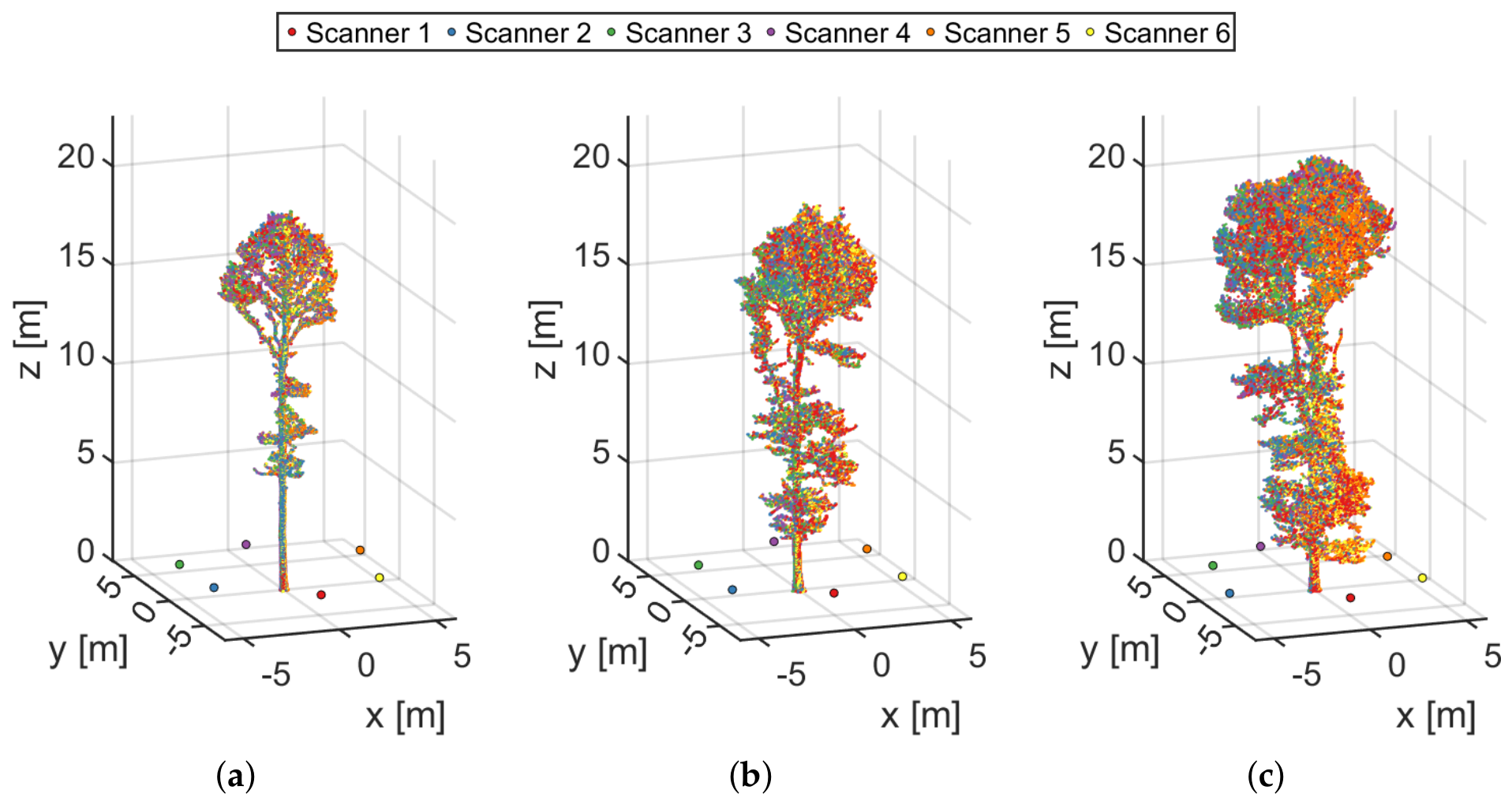
Scanner noise, multiple reflections, and ghost points were detected using a depth-discontinuity triangle-based method, using the angle between the local surface normal and the laser scanner’s viewing direction [39,40]. The resulting filtered point clouds were co-registered using Cyclone v9.0 (Leica Geosystems Ltd., Heerbrugg, Switzerland), based on six 6″ reflective planar targets positioned around each tree. The final co-registered point clouds are shown in Figure 1.

3. Methodology

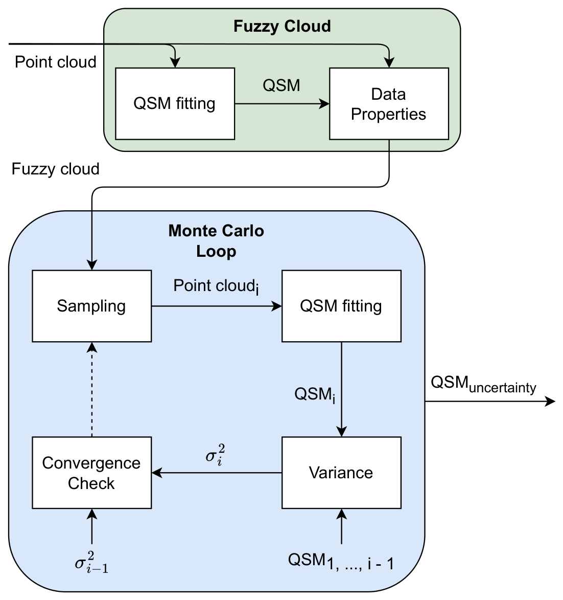
This section describes the procedure to determine the uncertainty of a QSM reconstructed from a point cloud of a tree. First, the point cloud together with the known scanner locations is used along with an initial geometry estimate to determine the uncertainty of each point. The details of forming point-wise uncertainty distributions is described in Section 3.1. Once the uncertainty distribution of each point is known, they are sampled in a Monte Carlo loop to propagate measurement uncertainty into the uncertainty of the QSM, as described in Section 3.2. A flowchart of the method is shown in Figure 2. It should be noted that the presented methodology is developed with the aim of determining the precision of a QSM fitting methodology’s results, and thus not whether the values are close to the true ones.

3.1. Fuzzy Cloud

The first step is to quantify the uncertainty within the point cloud data and create a so-called fuzzy cloud [41]. Each point is no longer seen as discrete, but represented by a three-dimensional Gaussian. The source of this uncertainty is the finite beamwidth of the laser beam, within which the laser beam power follows a Gaussian distribution which results in a Gaussian point uncertainty [31]. The initial exit diameter of the beam covering one standard deviation is d 0 and increases approximately linearly along range R (distance between scanner s ^ and point x ^ ) according to the beam divergence half-angle λ , resulting in a standard deviation in the radial direction σ radial
σ radial ( x ^ | s ^ , d 0 , λ ) = 1 2 d 0 + R ( x ^ | s ^ ) tan ( λ ) .
The range uncertainty σ r a n g e can be thought of as a projection of the radial uncertainty on the geometry G and is thus dependent on the incidence angle α . Taking an empirically derived relation for the base-level range uncertainty of the device σ 0 ( R ) and assuming the incidence angle to be constant across the beam, the standard deviation is given by Equation (2). For the Leica HDS-6100, σ 0 ( R ) ranges from 0.5 to 2 mm at a range of 5 to 50 m (60% albedo at 650–690 nm). We note that lim α π / 2 tan ( α ) = ; however, as the energy returned to the scanner goes to zero for oblique hits, these points are not registered in reality.
σ range ( x ^ | s ^ , d 0 , λ , G ) = σ 0 ( R ) + σ radial ( x ^ | s ^ , d 0 , λ ) tan ( α ( x ^ | G ) ) .
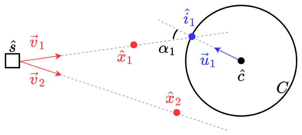
The incidence angle is the angle between the laser beam vector v going from scanner s ^ to point x ^ , and the vector normal to the surface where it intersects. Figure 3 shows two vectors, of which v 1 intersects the circle and thus allows for direct computation of α 1 . However, vectors may not intersect the geometry or have an unrealistically large incidence angle, for instance, due to poor geometry estimation or the beam having hit multiple objects (multiple branches of the tree). We therefore use a maximum incidence angle for these cases. This value is dependent on scanner hit registration and the object’s reflectivity—both of which are unknown for this study—and the range [42]. The maximum incidence angle can be estimated at the nearest parts of the stem and was found to be close to the maximum of 90°; however, such an estimate is not possible for parts further from the scanner. As such, we use a more conservative maximum of 80°.
To generalise the approach without prior knowledge of the true geometry, an initial QSM estimate is used to inform the incidence angles. We note that the uncertainty in fitting the initial QSM results in uncertainty in the incidence angles and thus affects the final results.

3.2. Monte Carlo Loop

Each distribution can be considered as the probabilistic region where a measurement has taken place. Therefore, once the fuzzy cloud is known, it can be sampled randomly to generate a new set of measurements (point cloud) to which a new QSM can be fitted. During sampling, the number of points does not change; instead, it can be thought of as a translation of each point. It should be noted that, in all practical cases, the original point cloud is already noisy and thus this step introduces a second layer of noise.
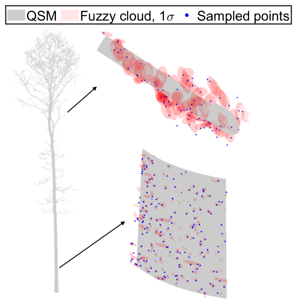
This sampling is illustrated in Figure 4, using the small tree with all scanners’ point clouds as an example. The section located at breast-height illustrates that the magnitude and orientation of the distributions coming from the different scanners differs greatly, but also that the size of the uncertainty is minor relative to the stem radius. On the other hand, the smaller branch has uncertainty on a similar magnitude to its radius. This branch also has multiple outliers, necessitating the aforementioned approach when there is no intersection between beam and geometry.
By repeating this sampling process in a Monte Carlo loop, the uncertainty from the fuzzy cloud can be propagated to the QSM. In this way, the uncertainty of global tree parameters such as the total volume and branch order-dependent parameters such as the volume of first-order branches can be determined.
In order to determine when the Monte Carlo loop has converged, the second statistical moment variance, σ 2 , of tree metrics of particular interest are used, i.e., the stem and branch volume. When the difference between the current i and previous i 1 variance estimate Δ ν i over the given parameters d is below the threshold, defined in Equation (3), iteration stops.
Δ ν i = j = 1 d σ i , j 2 σ i 1 , j 2 σ i 1 , j 2 2
We note that this is a convergence threshold in the precision and not accuracy of these metrics, as determining the precision is the aim of this study.

4. Case Study

To create example results of uncertainty, the approach was applied to the oak laser scanning data. For QSM reconstruction the TreeQSM 2.4.1 software was used [12]. As TreeQSM is inherently stochastic, generating multiple QSMs for each point cloud and selecting the optimal one is recommended. In this study, we fit five models and use the mean distance from the point cloud to the stem and branches to select the optimal one. In a similar manner, the optimal input parameters for each original point cloud are selected by letting TreeQSM determine a suitable range of input parameters using the same mean distance.
As a measure of the point cloud uncertainty, we determine the geometric average of the radial and range uncertainty
σ ¯ = σ radial σ range .
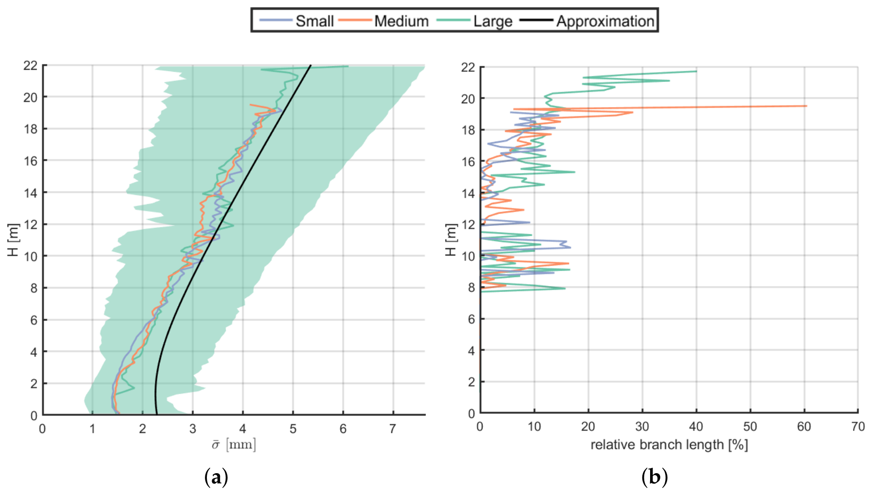
The relationship with the height is given in Figure 5a by taking the average within each 0.2 m bin. The 90% confidence interval ranges between 1 and 7.5 mm. Per the approximation derived in Appendix A, the mean value is roughly proportional to D S 2 + ( H H S ) 2 . Here, D S and H S are the distance between scanner and stem (≈5 m) and the height of the scanner (≈1.3 m), respectively. This equation shows that the relationship between σ ¯ and H becomes linear when H > D S , H S . We note, however, that this approximation may not be valid for other scanners and applications.
To illustrate the relevance of this uncertainty, Figure 5b shows the percentage of branch length that has a radius smaller than this geometric average uncertainty, and thus has a noise magnitude of the same magnitude as the geometry itself. For lower parts of the trees, this percentage does not exceed 20%; however, it increases with height and reaches a maximum of 60%. It should further be noted that in reality this percentage is expected to be higher, as smaller branches may be missed by the scanner or reconstruction approach.
With TreeQSM, it is not possible to evaluate the uncertainty of individual cylinders or even necessarily branches, as the fitted topology is not guaranteed to be the same. Instead, aggregated results are shown subsequently: those for the tree as a whole (Section 4.1) and ones for specific branch orders (Section 4.2). These results were determined using a hundred iterations, but we remind the reader that the uncertainty given here is over-estimated due to the original point cloud already being noisy. As six scanners were placed around each tree roughly 60 degrees apart from each other, indirectly the effect of occlusion on volume and length and their uncertainty could be studied by testing four scanning configurations: a single scanner (1), two scanners on opposite sides (1 and 4), four scanners with two on each side (1, 2, 4 and 5) and all scanners (1 through 6).

4.1. Tree Parameters

In this section, we report the results for the total volume of the tree and that of the stem and branches using the data from a hundred iterations. Similar analysis was carried out for the rest of the tree-level parameters that TreeQSM determines, but are omitted here for brevity. For each combination of size and scanner location, the mean and relative standard deviations of the volumes are tabulated in Table 1. In addition, the histograms are presented in Appendix B.
Increasing the number of scanner locations increases the number of data points and decreases occlusion [32]. Correspondingly, the ability to reconstruct QSMs improves, and the uncertainty generally decreases with the number of scanner locations. The relative uncertainty of the stem is generally smaller than of the branches, indicating a greater reconstructability for the stem. Similarly, as the percentage of the tree which is scanned increases, one can logically expect the estimated volume to increase accordingly, especially branch volume, as branches suffer more from occlusion [32]. This is, however, not universally the case with both the small and medium trees having the largest branch volume for two opposite scanner locations.
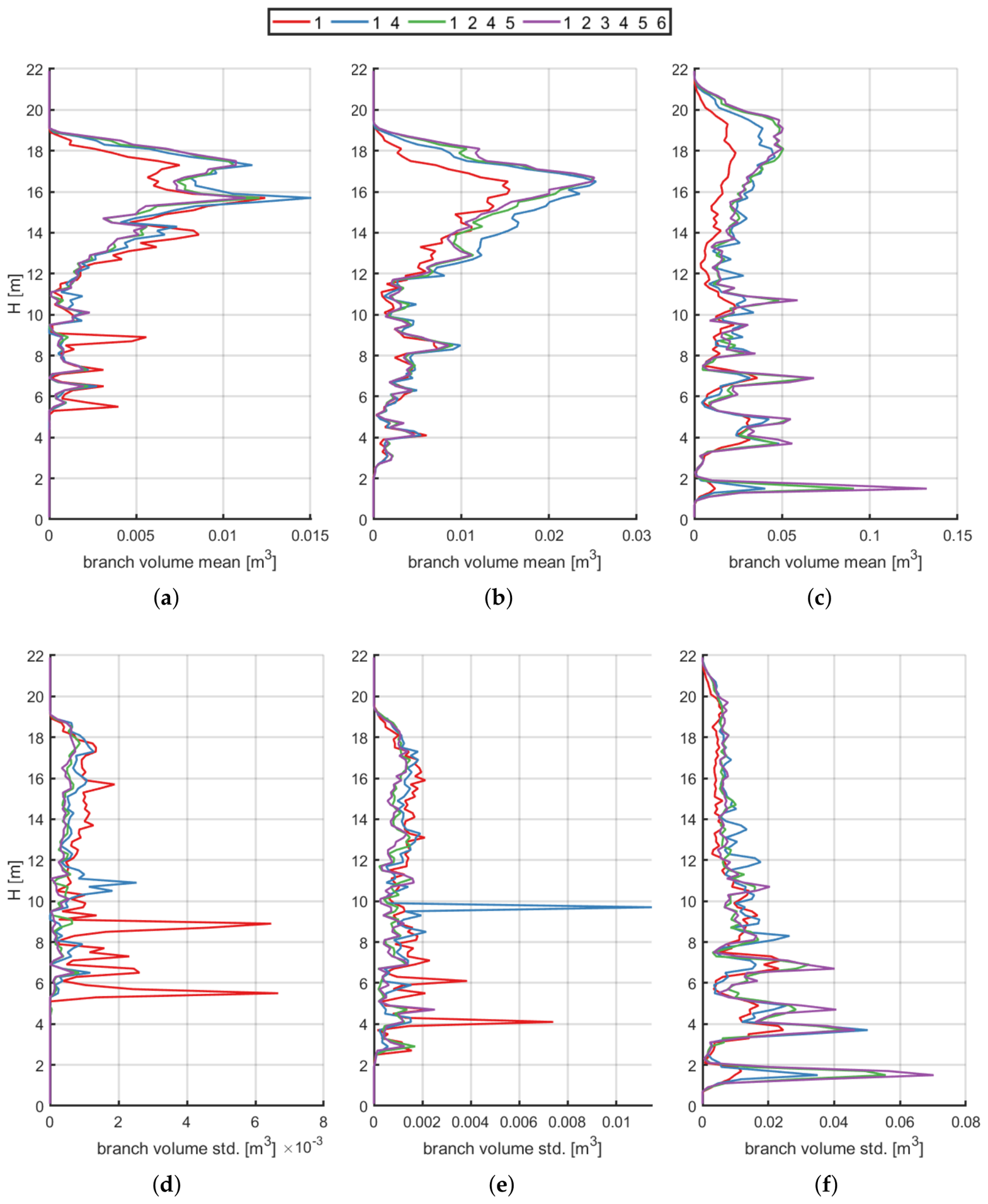
An explanation for this can be found when plotting the mean and standard deviation of the branch volume in terms of height within 0.2 m bins, as shown in Figure 6. We would generally expect the mean value and standard deviation to increase with height, the former because there are more branches in the crown and the latter because this results in greater occlusion and the distance to the scanner increases reducing data quality. Whilst this trend can somewhat be observed for the small and medium-sized trees, TreeQSM commonly struggled to fit branches below the crown, resulting in high uncertainty.

4.2. Branch Parameters

We can further analyse the tree metrics by determining their distributions within the branch orders, again for a hundred iterations. It should be noted that, with approaches such as TreeQSM where cylinder fitting starts from the stem and then continues down the branches, uncertainty of lower branch orders is inherently propagated to that of higher branch orders. Additionally, with TreeQSM, the topology between models is not guaranteed to be the same, and thus neither are n-th order branches. The uncertainty in metrics is therefore not just because of data uncertainty, but also TreeQSM stochasticity.
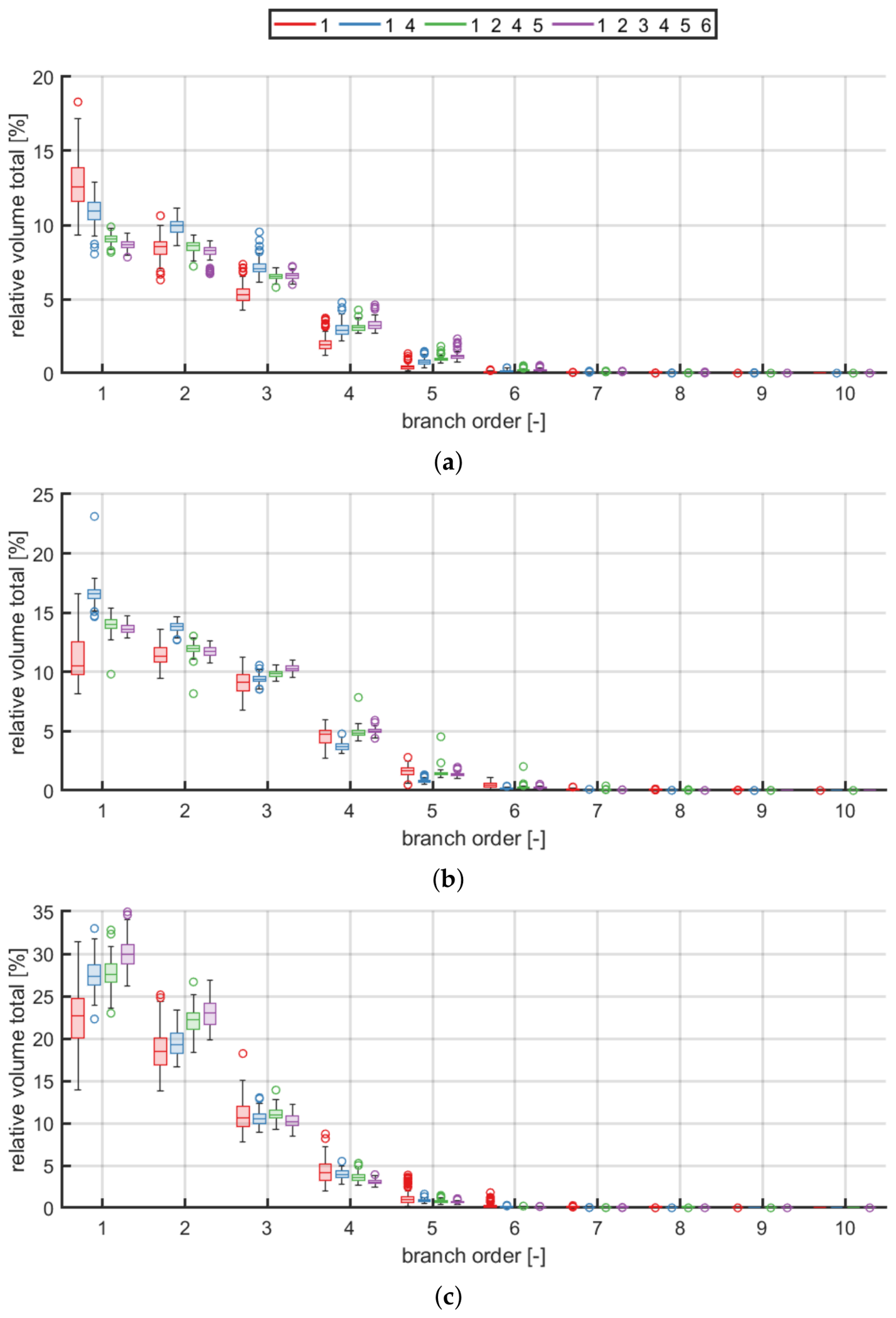
Figure 7 shows that the contribution of higher branch orders (>6) to the total volume, both in terms of mean and standard deviation, is negligible. As noted previously, the volume does not universally increase with increasing scanner locations.
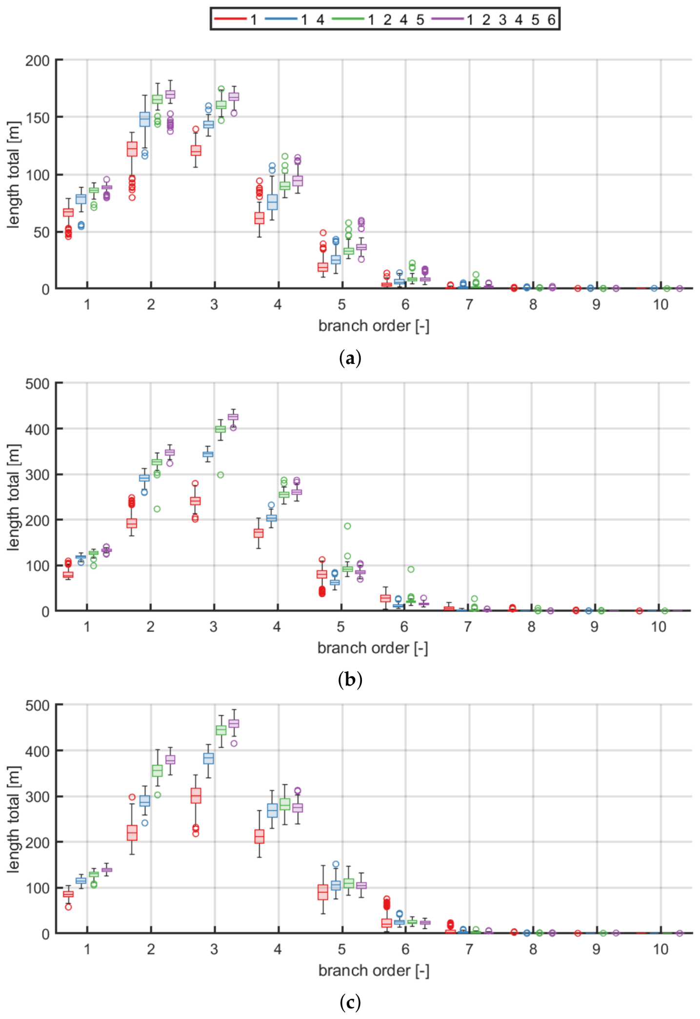
Aside from the volume, other metrics such as the total branch length shown in Figure 8 can be analysed. Contrary to the volume, the branch length consistently increases with increasing scanner locations for all three trees. Over-estimation of the radius for poor data quality was found by prior studies, so this may be indicative of an increase in length being counter-acted by an improvement in radius estimation [24,43,44]. As our estimate of the point cloud uncertainty is dependent on the incidence angle and thus the radius, the sensitivity of tree metric uncertainty to radius bias was estimated by adjusting all initial QSM radii by a factor between −20% and 20% and running the Monte Carlo loop. No conclusive relationship was found, with only a reduction of 0.04% for the total volume and branch volume standard deviations. This indicates that the approach is robust to small bias in initial geometry estimates in our test case.

4.3. Convergence

Convergence is determined by checking the similarity of subsequent variance estimates Δ ν for three tree parameters: stem volume, branch volume, and branch length using Equation (3). To more robustly determine the number of iterations until convergence, a hundred random permutations of the QSMs and thus tree parameters were tested. Table 2 shows the average iteration at which convergence was determined as well as the percentage of permutations for which convergence could not be established.
It should be noted that incomplete knowledge, for instance, of the true geometry and reflectance properties of the tree, limits our ability to accurately estimate the acceptable variance levels for the subsequent tree parameters. The authors therefore believe the effectiveness of setting the variance threshold low to be limited.
When the threshold is 5 % , all data sets converged on average within 25 iterations and all converged well within the hundred iterations. When the threshold is stricter at 1 % , convergence on average occurred within 82 iterations. While the majority converged within a hundred iterations, convergence can no longer be guaranteed and at most 18 % of the tested permutations exceeded the threshold.
We note that metric estimates converge more rapidly than the variance. The mean relative absolute difference between the full series and those limited by a 5 % convergence threshold was found to be less than 0.5%, converging more rapidly with a greater number of scanners.
As the computational cost increases approximately linearly with the number of iterations, we thus estimate uncertainty quantification to increase the computational cost by 25 times compared to fitting a single QSM for a 5% threshold.

5. Discussion

Our results demonstrate that uncertainties in tree-level metrics arising from noise and measurement variability in TLS data can be quantitatively assessed rather than treated as unknown. By propagating data-level uncertainty through the reconstruction and metric-extraction workflow, we show that the reliability of TLS- and QSM-derived estimates can be explicitly characterized. This capability is valuable for both forestry practice and forest science, where decisions and model predictions increasingly rely on precise structural information. Quantifying uncertainty provides practitioners with clearer confidence bounds for operational metrics and strengthens the robustness and interpretability of research outcomes based on TLS measurements.
The aim of the methodology was to be applicable to any QSM reconstruction approach and to the data of any tree. As such, it is a high-level approach whereby Monte Carlo simulation is favoured over more specific analytical or numerical approaches and uncertainty is determined using only the point cloud and an initial geometry estimate. Whilst the approach is thus expected to be broadly applicable, we only demonstrated it using TreeQSM applied to three English oaks and thus cannot guarantee its validity in other applications. Particular challenges would come from situations where the source of each data point on the tree and thus the point’s uncertainty cannot be determined accurately, for instance, when leaves are present for coniferous and tropical trees or when the forest and tree structure are highly complex.
It is important to note that, by sampling the noisy input data, another layer of noise is added. As a result, the uncertainty of the QSM determined by the approach outlined in this article is an over-estimation. While not practical for real applications as it requires knowledge of the tree geometry, this over-estimation can be avoided by creating a model of this tree and simulating laser scanning on it without noise to produce the initial point cloud, i.e., by using Helios + + [45]. Furthermore, we used a constant maximum incidence angle of 80° whilst in reality this is dependent on many factors such as material properties and range [42]. Nearer distributions are thus likely under-estimated and farther over-estimated. Future studies may instead want to estimate the maximum incidence angle at different ranges using accurately fitted parts of the tree for which partial hits are unlikely.
It should further be noted that TreeQSM is an inherently stochastic reconstruction approach [12] and deterministic approaches are thus likely to have lower uncertainty. Additionally, TreeQSM fits connected branches dependently, which means that uncertainty estimates are similarly dependent. The uncertainty of the fitting approach can be quantified by fitting a large number of QSMs to the same point cloud (i.e., foregoing resampling). Alternatively, TreeQSM can be made non-stochastic by making the segmentation constant within the Monte Carlo loop such that the same point cloud subset is used for each cylinder fit.
The effects of this stochasticity in the form of reconstruction errors were also evident in the volume not universally increasing when more scanners were added, despite a greater fraction of the tree then being covered by data. These errors can be detected manually, but doing so introduces subjectivity and is laborious when a large number of QSMs need to be fitted to quantify the uncertainty. Instead, automated detection of outlier QSMs may be possible, and these outliers discarded, to reduce the effects of reconstruction errors on the uncertainty estimate. Either way, if a regular workflow involves the removal of outlier QSMs, this step would need to be incorporated into the Monte Carlo loop for the uncertainty estimates to be representative.
We presume sampling (i.e., laser scanning points) to be independent, but in reality, dependence is introduced through systematic errors and post-processing performed by the scanning instruments. Modelling these errors requires extensive knowledge of the scanner and careful laboratory testing [3,46]. Meanwhile, the post-processing algorithms are generally not publicly available.
Another shortcoming of our uncertainty model is that it assumes constant incidence angle within the beam, which is a poor assumption for small branches. A possibility is to subdivide each distribution and assume constant incidence angle within each part. The computational cost increases accordingly; however, it may be reduced by making the degree of subdivision inversely proportional to the branch radius.
Currently, we do not take uncertainty arising from co-registration into account. If reflective targets are used for co-registration, the uncertainty of each measurement of the target can be propagated with relative simplicity to the uncertainty of the target location. For alternative target-free approaches that use structures within the point cloud such as [47], determining the co-registration uncertainty is more complex, but may be achieved by methods such as Monte Carlo simulation. The translational and rotational uncertainty of co-registration can be added to the location uncertainty of each point within the point cloud, and thus propagated to the QSM uncertainty using the method described in this article. Analysing the uncertainty of co-registration is an interesting avenue for future research.
Alternative convergence criteria for the Monte Carlo loop would be to fit distributions and measure their similarity using the Bhattacharyya distance [48]. If Hartigan’s dip test [49] indicates the underlying distribution to be uni-modal, a multivariate Gaussian can be fitted. Alternatively, a mixture model is more appropriate. It should be noted however that these distributions are dependent on a larger number of parameters and may converge more slowly.
Finally, we note the challenges that come with validating uncertainty quantification and welcome future studies to experimentally quantify the uncertainty of tree metrics and validate the uncertainty quantified by the presented approach. Such experiments may be conducted in a controlled environment where repeated measurements can be taken without external interference and ideally of a tree whose exact geometry is known.

6. Conclusions

Uncertainty in tree metrics derived from LiDAR data is not commonly assessed, yet our results show that these uncertainties can be substantial and therefore merit greater attention. In this study, we introduced a straightforward method to propagate the uncertainty resulting from the finite beamwidth of terrestrial laser scanning data to quantitative structure model (QSM)-derived metrics. The approach first transforms the original point cloud into a fuzzy cloud by accounting for the effects of beamwidth and incidence angle on measurement accuracy, allowing uncertainty to vary in both magnitude and shape from point to point. Point clouds are then repeatedly sampled from this fuzzy cloud in a Monte Carlo framework, and a QSM is reconstructed for each sample to propagate the uncertainty into the resulting tree metrics. Convergence is monitored by comparing variance estimates across iterations. We demonstrated the method on three trees of varying size under four scanning configurations. The results showed that uncertainty decreases as the number of scanner positions increases—particularly for small branches—and that stems generally exhibit lower relative uncertainty than branches. These findings exemplify how the uncertainty in TLS- and QSM-derived tree metrics can be effectively quantified, providing transparent insight into the reliability of structural estimates. Although our demonstration focused on a limited set of trees and scanning setups, the method offers a flexible framework that can be applied more broadly. We encourage future studies to test it with different scanners, species, or full forest plots and to extend the uncertainty model. More generally, incorporating uncertainty quantification into forestry and forest research would strengthen the robustness of analyses, support more informed decision-making, and improve confidence in structural metrics increasingly used in both scientific and operational contexts.

Author Contributions

Conceptualization, V.B.V.; methodology, V.B.V. and E.C.; software, V.B.V.; validation, V.B.V.; formal analysis, V.B.V. and E.C.; investigation, V.B.V.; resources, V.B.V. and E.C.; data acquisition and curation, E.C.; writing—original draft preparation, V.B.V.; writing—review and editing, V.B.V., E.C., M.Å. and P.R.; visualization, V.B.V.; supervision, E.C., M.Å. and P.R.; project administration, P.R.; funding acquisition, E.C. and P.R. All authors have read and agreed to the published version of the manuscript.

Funding

This research has been supported by Research Council of Finland (Centre of Excellence of Inverse Modelling and Imaging, grant 353090, and Flagship of Advanced Mathematics for Sensing Imaging and Modelling, grant 359185) and the UK Department for Environment, Food and Rural Affairs and by Forest Research, GB.

Data Availability Statement

The TLS data of the oak trees is available upon request from E. Casella eric.casella@forestresearch.gov.uk, and the code is available from https://github.com/InverseTampere/UncertainTreeQSM (accessed on 14 June 2026).

Acknowledgments

E. Casella acknowledges Ian Craig for his participation in the oak tree TLS measurements.

Conflicts of Interest

Author Markku Åkerblom was employed by the Patria Aviation Oy. The remaining authors declare that the research was conducted in the absence of any commercial or financial relationships that could be construed as a potential conflict of interest.

Appendix A. Approximate Relationship Between Height and Average Uncertainty

The aim is to derive a simple relationship between the average uncertainty σ ¯ and the height along the tree H. We note that the assumptions made here are not intended to be rigorous or generally applicable. First, inserting Equation (2) into Equation (4) leads to
σ ¯ = σ radial σ range = σ radial ( σ 0 ( R ) + σ radial tan ( α ) ) .
This equation contains the empirical relation for σ 0 ( R ) and is non-linear with respect to σ radial and thus range R. If we use the rough approximation that σ 0 ( R ) σ radial , we instead have
σ ¯ σ radial 1 + tan ( α )
Inserting Equation (1) splits the equation into a constant part and one dependent on range R:
σ ¯ d 0 2 + R tan ( λ ) 1 + tan ( α ) .
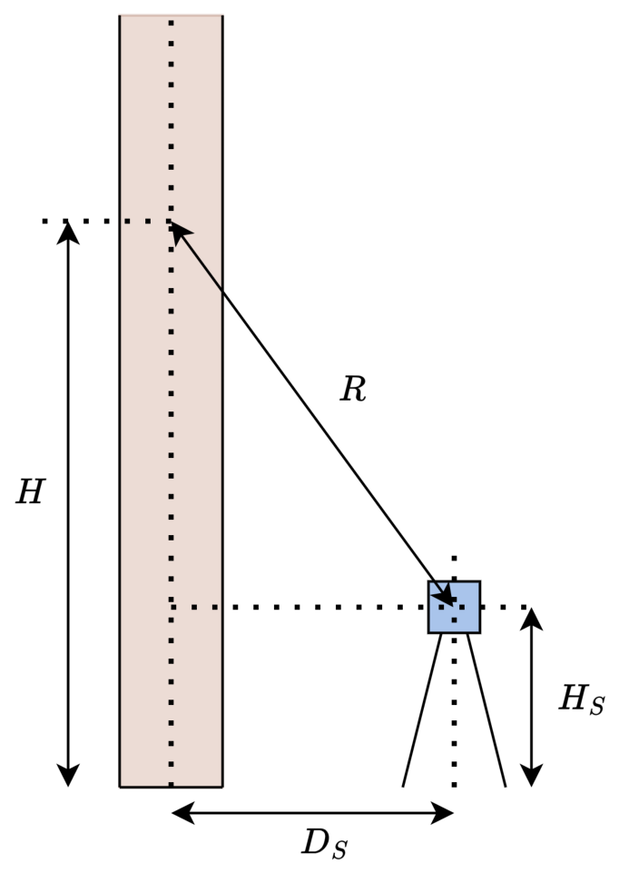
The distribution of the incidence angle α is assumed to be independent of height, and therefore tan ( α ) is substituted by the average found for the assessed data; E [ tan ( α ) ] 2 . Additionally, defining D S and H S to be the distance between the scanner and tree centre line and height of the scanner respectively as shown in Figure A1, we derive the relationship R ( H | D S , H S ) = D S 2 + ( H H S ) 2 and show that
σ ¯ ( H | D S , H S , d 0 , λ ) 3 d 0 2 + 3 tan ( λ ) D S 2 + ( H H S ) 2 .
Figure A1. Illustration to show the relationship between the range R and height H.
Remotesensing 18 02005 g0a1

Appendix B. Tree Parameters

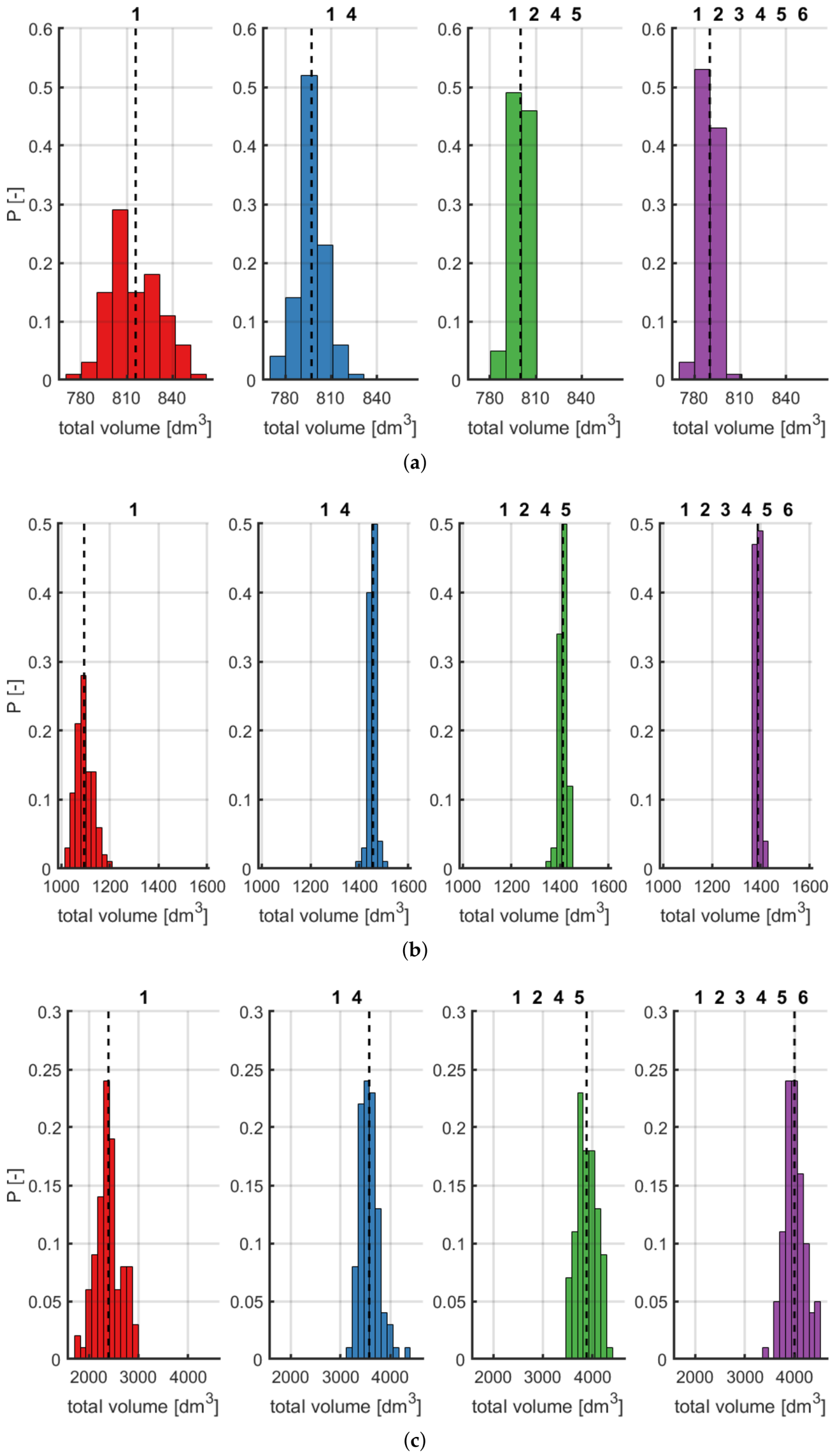
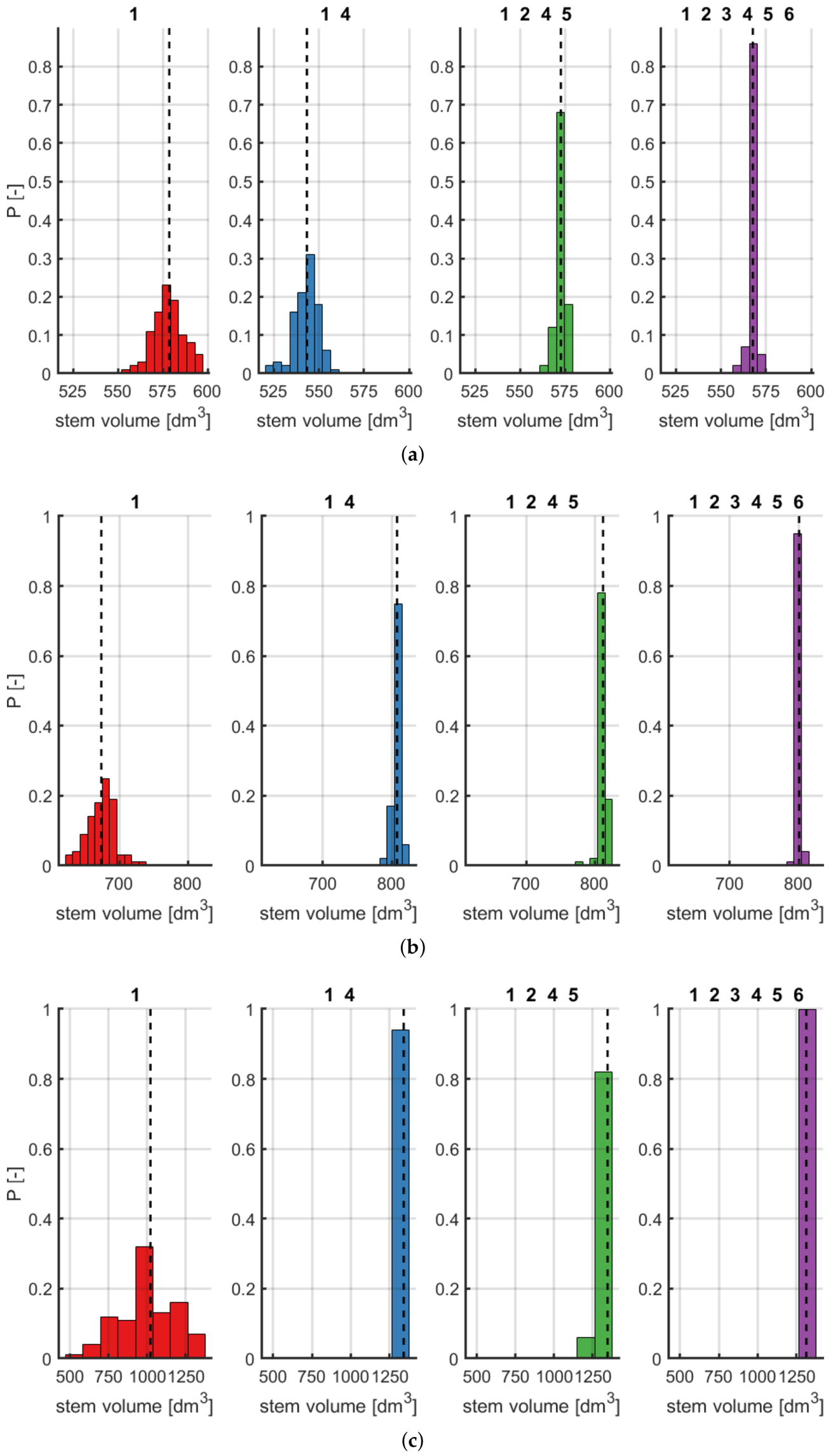
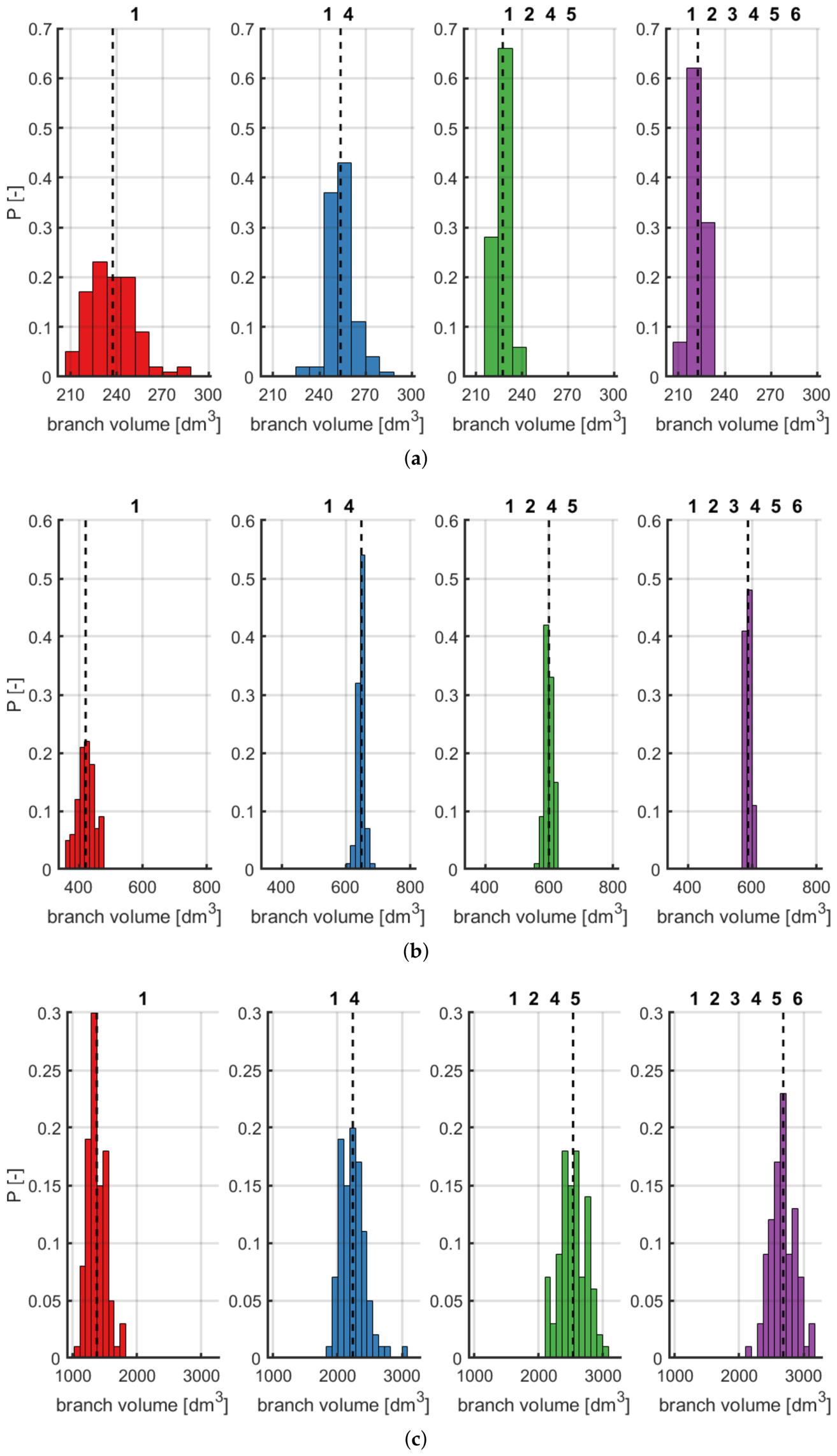
Histograms are given for the tree parameters analysed in Section 4.1; the total tree volume (Figure A2), stem volume (Figure A3), and branch volume (Figure A4).
Figure A2. Total volume distribution for the (a) small, (b) medium and (c) large trees. Mean values are shown with the dashed lines.
Remotesensing 18 02005 g0a2
Figure A3. Stem volume distribution for the (a) small, (b) medium and (c) large trees. Mean values are shown with the dashed lines.
Remotesensing 18 02005 g0a3
Figure A4. Branch volume distribution for the (a) small, (b) medium and (c) large trees. Mean values are shown with the dashed lines.
Remotesensing 18 02005 g0a4

References

  1. Shukla, P.; Skea, J.; Calvo Buendia, E.; Masson-Delmotte, V.; Pörtner, H.; Roberts, D.; Zhai, P.; Slade, R.; Connors, S.; Van Diemen, R.; et al. Climate Change and Land: An IPCC Special Report on Climate Change, Desertification, Land Degradation, Sustainable Land Management, Food Security, and Greenhouse Gas Fluxes in Terrestrial Ecosystems; Technical Report; Intergovernmental Panel on Climate Change (IPCC): Geneva, Switzerland, 2019. [Google Scholar]
  2. Bonan, G.B. Forests and climate change: Forcings, feedbacks, and the climate benefits of forests. Science 2008, 320, 1444–1449. [Google Scholar] [CrossRef] [PubMed]
  3. Vosselman, G.; Maas, H.G. Airborne and Terrestrial Laser Scanning; Whittles Publishing: Scotland, UK, 2010. [Google Scholar]
  4. Hashimoto, H.; Imanishi, J.; Hagiwara, A.; Morimoto, Y.; Kitada, K. Estimating forest structure indices for evaluation of forest bird habitats by an airborne laser-scanner. In Proceedings of the ISPRS Working Group VIII/2 Laser-Scanners for Forest and Landscape Assessment, Freiburg, Germany, 3–6 October 2004; Citeseer: University Park, PA, USA, 2004; pp. 254–257. [Google Scholar]
  5. Vihervaara, P.; Mononen, L.; Auvinen, A.P.; Virkkala, R.; Lü, Y.; Pippuri, I.; Packalen, P.; Valbuena, R.; Valkama, J. How to integrate remotely sensed data and biodiversity for ecosystem assessments at landscape scale. Landsc. Ecol. 2015, 30, 501–516. [Google Scholar] [CrossRef]
  6. Åkerblom, M.; Raumonen, P.; Mäkipää, R.; Kaasalainen, M. Automatic tree species recognition with quantitative structure models. Remote Sens. Environ. 2017, 191, 1–12. [Google Scholar] [CrossRef]
  7. Gobakken, T.; Næsset, E. Effects of forest growth on laser derived canopy metrics. Int. Arch. Photogramm. Remote Sens. Spat. Inf. Sci. 2004, 36, 224–227. [Google Scholar]
  8. Hyyppä, J.; Hyyppä, H.; Litkey, P.; Yu, X.; Haggrén, H.; Rönnholm, P.; Pyysalo, U.; Pitkänen, J.; Maltamo, M. Algorithms and methods of airborne laser scanning for forest measurements. Int. Arch. Photogramm. Remote Sens. Spat. Inf. Sci. 2004, 36, 82–89. [Google Scholar]
  9. Stephens, P.; Watt, P.; Loubser, D.; Haywood, A.; Kimberley, M. Estimation of carbon stocks in New Zealand planted forests using airborne scanning LiDAR. Int. Arch. Photogramm. Remote Sens. Spat. Inf. Sci. 2007, 36, 389–394. [Google Scholar]
  10. Wang, D.; Puttonen, E.; Casella, E. PlantMove: A tool for quantifying motion fields of plant movements from point cloud time series. Int. J. Appl. Earth Obs. Geoinf. 2022, 110, 102781. [Google Scholar] [CrossRef]
  11. Maeda, E.E.; Brede, B.; Calders, K.; Disney, M.; Herold, M.; Lines, E.R.; Nunes, M.H.; Raumonen, P.; Rautiainen, M.; Saarinen, N.; et al. Expanding forest research with terrestrial LiDAR technology. Nat. Commun. 2025, 16, 8853. [Google Scholar] [CrossRef] [PubMed]
  12. Raumonen, P.; Kaasalainen, M.; Åkerblom, M.; Kaasalainen, S.; Kaartinen, H.; Vastaranta, M.; Holopainen, M.; Disney, M.; Lewis, P. Fast automatic precision tree models from terrestrial laser scanner data. Remote Sens. 2013, 5, 491–520. [Google Scholar] [CrossRef]
  13. Du, S.; Lindenbergh, R.; Ledoux, H.; Stoter, J.; Nan, L. AdTree: Accurate, detailed, and automatic modelling of laser-scanned trees. Remote Sens. 2019, 11, 2074. [Google Scholar] [CrossRef]
  14. Hackenberg, J.; Spiecker, H.; Calders, K.; Disney, M.; Raumonen, P. SimpleTree—an efficient open source tool to build tree models from TLS clouds. Forests 2015, 6, 4245–4294. [Google Scholar] [CrossRef]
  15. Casella, E.; Sinoquet, H. A method for describing the canopy architecture of coppice poplar with allometric relationships. Tree Physiol. 2003, 23, 1153–1170. [Google Scholar] [CrossRef] [PubMed]
  16. Raumonen, P.; Åkerblom, M. TreeQSM. 2022. Available online: https://github.com/InverseTampere/TreeQSM?rev=cb02264ffcbd4123b82a5c42f29b14be (accessed on 17 May 2022).
  17. Calders, K.; Newnham, G.; Burt, A.; Murphy, S.; Raumonen, P.; Herold, M.; Culvenor, D.; Avitabile, V.; Disney, M.; Armston, J.; et al. Nondestructive estimates of above-ground biomass using terrestrial laser scanning. Methods Ecol. Evol. 2015, 6, 198–208. [Google Scholar] [CrossRef]
  18. Yang, W.; Wilkes, P.; Vicari, M.B.; Hand, K.; Calders, K.; Disney, M. Treegraph: Tree architecture from terrestrial laser scanning point clouds. Remote Sens. Ecol. Conserv. 2024, 10, 755–774. [Google Scholar] [CrossRef]
  19. Feng, Y.; Su, Y.; Wang, J.; Yan, J.; Qi, X.; Maeda, E.E.; Nunes, M.H.; Zhao, X.; Liu, X.; Wu, X.; et al. L1-Tree: A novel algorithm for constructing 3D tree models and estimating branch architectural traits using terrestrial laser scanning data. Remote Sens. Environ. 2024, 314, 114390. [Google Scholar] [CrossRef]
  20. Boehler, W.; Vicent, M.B.; Marbs, A. Investigating laser scanner accuracy. Int. Arch. Photogramm. Remote Sens. Spat. Inf. Sci. 2003, 34, 696–701. [Google Scholar]
  21. Schaer, P.; Skaloud, J.; Landtwing, S.; Legat, K. Accuracy estimation for laser point cloud including scanning geometry. In Proceedings of the Mobile Mapping Symposium 2007, Istanbul, Turkey, 13–15 June 2007. [Google Scholar]
  22. Calders, K.; Disney, M.I.; Armston, J.; Burt, A.; Brede, B.; Origo, N.; Muir, J.; Nightingale, J. Evaluation of the range accuracy and the radiometric calibration of multiple terrestrial laser scanning instruments for data interoperability. IEEE Trans. Geosci. Remote Sens. 2017, 55, 2716–2724. [Google Scholar] [CrossRef]
  23. Lichti, D.D.; Gordon, S.J.; Tipdecho, T. Error models and propagation in directly georeferenced terrestrial laser scanner networks. J. Surv. Eng. 2005, 131, 135–142. [Google Scholar] [CrossRef]
  24. Morhart, C.; Schindler, Z.; Frey, J.; Sheppard, J.P.; Calders, K.; Disney, M.; Morsdorf, F.; Raumonen, P.; Seifert, T. Limitations of estimating branch volume from terrestrial laser scanning. Eur. J. For. Res. 2024, 143, 687–702. [Google Scholar] [CrossRef]
  25. Bloom, A.A.; Exbrayat, J.F.; Van Der Velde, I.R.; Feng, L.; Williams, M. The decadal state of the terrestrial carbon cycle: Global retrievals of terrestrial carbon allocation, pools, and residence times. Proc. Natl. Acad. Sci. USA 2016, 113, 1285–1290. [Google Scholar] [CrossRef] [PubMed]
  26. Friend, A.D.; Lucht, W.; Rademacher, T.T.; Keribin, R.; Betts, R.; Cadule, P.; Ciais, P.; Clark, D.B.; Dankers, R.; Falloon, P.D.; et al. Carbon residence time dominates uncertainty in terrestrial vegetation responses to future climate and atmospheric CO2. Proc. Natl. Acad. Sci. USA 2014, 111, 3280–3285. [Google Scholar] [CrossRef] [PubMed]
  27. Disney, M.I.; Boni Vicari, M.; Burt, A.; Calders, K.; Lewis, S.L.; Raumonen, P.; Wilkes, P. Weighing trees with lasers: Advances, challenges and opportunities. Interface Focus 2018, 8, 20170048. [Google Scholar] [CrossRef] [PubMed]
  28. Wang, Y.; Lehtomäki, M.; Liang, X.; Pyörälä, J.; Kukko, A.; Jaakkola, A.; Liu, J.; Feng, Z.; Chen, R.; Hyyppä, J. Is field-measured tree height as reliable as believed—A comparison study of tree height estimates from field measurement, airborne laser scanning and terrestrial laser scanning in a boreal forest. ISPRS J. Photogramm. Remote Sens. 2019, 147, 132–145. [Google Scholar] [CrossRef]
  29. Kükenbrink, D.; Gardi, O.; Morsdorf, F.; Thürig, E.; Schellenberger, A.; Mathys, L. Above-ground biomass references for urban trees from terrestrial laser scanning data. Ann. Bot. 2021, 128, 709–724. [Google Scholar] [CrossRef] [PubMed]
  30. Momo Takoudjou, S.; Ploton, P.; Sonké, B.; Hackenberg, J.; Griffon, S.; De Coligny, F.; Kamdem, N.; Libalah, M.; Mofack, G.; Le Moguédec, G.; et al. Using terrestrial laser scanning data to estimate large tropical trees biomass and calibrate allometric models: A comparison with traditional destructive approach. Methods Ecol. Evol. 2018, 9, 905–916. [Google Scholar] [CrossRef]
  31. Hartzell, P.J.; Gadomski, P.J.; Glennie, C.L.; Finnegan, D.C.; Deems, J.S. Rigorous error propagation for terrestrial laser scanning with application to snow volume uncertainty. J. Glaciol. 2015, 61, 1147–1158. [Google Scholar] [CrossRef]
  32. Wilkes, P.; Lau, A.; Disney, M.; Calders, K.; Burt, A.; de Tanago, J.G.; Bartholomeus, H.; Brede, B.; Herold, M. Data acquisition considerations for terrestrial laser scanning of forest plots. Remote Sens. Environ. 2017, 196, 140–153. [Google Scholar] [CrossRef]
  33. Suchocki, C. Comparison of time-of-flight and phase-shift TLS intensity data for the diagnostics measurements of buildings. Materials 2020, 13, 353. [Google Scholar] [CrossRef] [PubMed]
  34. Muralikrishnan, B. Performance evaluation of terrestrial laser scanners—A review. Meas. Sci. Technol. 2021, 32, 072001. [Google Scholar] [CrossRef] [PubMed]
  35. Wan, P.; Wang, T.; Zhang, W.; Liang, X.; Skidmore, A.K.; Yan, G. Quantification of occlusions influencing the tree stem curve retrieving from single-scan terrestrial laser scanning data. For. Ecosyst. 2019, 6, 43. [Google Scholar] [CrossRef]
  36. Li, L.; Mu, X.; Soma, M.; Wan, P.; Qi, J.; Hu, R.; Zhang, W.; Tong, Y.; Yan, G. An Iterative-Mode Scan Design of Terrestrial Laser Scanning in Forests for Minimizing Occlusion Effects. IEEE Trans. Geosci. Remote Sens. 2020, 59, 3547–3566. [Google Scholar] [CrossRef]
  37. Raumonen, P.; Casella, E.; Calders, K.; Murphy, S.; Åkerblom, M.; Kaasalainen, M. Massive-scale tree modelling from TLS data. ISPRS Ann. Photogramm. Remote Sens. Spat. Inf. Sci. 2015, 2, 189–196. [Google Scholar] [CrossRef]
  38. Leica Geosystems. Leica HDS6100. Available online: https://downloads.leica-geosystems.com/files/archived-files/hds6100_datasheet_us.pdf (accessed on 8 December 2025).
  39. Rombourg, R. Terrestrial Laser Scanner Noise Analysis, Modelling and Detection. Ph.D. Thesis, Domaine Universitaire de Saint-Martin-d’Hères, Grenoble, France, 2019. [Google Scholar]
  40. Tang, P.; Huber, D.; Akinci, B. A comparative analysis of depth-discontinuity and mixed-pixel detection algorithms. In Proceedings of the Sixth International Conference on 3-D Digital Imaging and Modeling (3DIM 2007), Montreal, QC, Canada, 21–23 August 2007; pp. 29–38. [Google Scholar]
  41. Verhoeven, V.B.; Raumonen, P.; Åkerblom, M. Fitting Geometric Shapes to Fuzzy Point Cloud Data. J. Imaging 2025, 11, 7. [Google Scholar] [CrossRef] [PubMed]
  42. Verhoeven, V.; Raumonen, P.; Åkerblom, M.; Tammi, K.; Tasanen, I. The Effect of Surface Material on Cylinder Point Clouds. IEEE Trans. Instrum. Meas. 2025, 74, 1010912. [Google Scholar] [CrossRef]
  43. Michałowska, M.; Rapiński, J.; Janicka, J. Tree position estimation from TLS data using hough transform and robust least-squares circle fitting. Remote Sens. Appl. Soc. Environ. 2023, 29, 100863. [Google Scholar] [CrossRef]
  44. Okatani, T.; Deguchi, K. On bias correction for geometric parameter estimation in computer vision. In Proceedings of the 2009 IEEE Conference on Computer Vision and Pattern Recognition, Miami, FL, USA, 20–25 June 2009; pp. 959–966. [Google Scholar]
  45. Winiwarter, L.; Pena, A.M.E.; Weiser, H.; Anders, K.; Sánchez, J.M.; Searle, M.; Höfle, B. Virtual laser scanning with HELIOS++: A novel take on ray tracing-based simulation of topographic full-waveform 3D laser scanning. Remote Sens. Environ. 2022, 269, 112772. [Google Scholar] [CrossRef]
  46. Abegg, M.; Boesch, R.; Schaepman, M.E.; Morsdorf, F. Impact of beam diameter and scanning approach on point cloud quality of terrestrial laser scanning in forests. IEEE Trans. Geosci. Remote Sens. 2020, 59, 8153–8167. [Google Scholar] [CrossRef]
  47. Castorena, J.; Dickman, L.T.; Killebrew, A.J.; Gattiker, J.R.; Linn, R.; Loudermilk, E.L. ForestAlign: Automatic forest structure-based alignment for multi-view TLS and ALS point clouds. Sci. Remote Sens. 2025, 11, 100194. [Google Scholar] [CrossRef]
  48. Bhattacharyya, A. On a measure of divergence between two multinomial populations. Sankhyā Indian J. Stat. 1946, 7, 401–406. [Google Scholar]
  49. Hartigan, J.A.; Hartigan, P.M. The dip test of unimodality. Ann. Stat. 1985, 13, 70–84. [Google Scholar] [CrossRef]
Figure 1. The point clouds of the (a) small, (b) medium and (c) large trees and scanner positions at the bottom of the stem.
Remotesensing 18 02005 g001
Figure 2. Flowchart for uncertainty quantification of the QSM. Solid arrows imply a direct connection, whilst the dashed arrow implies continuation of the Monte Carlo loop dependent on the convergence check.
Remotesensing 18 02005 g002
Figure 3. 2D illustration of two beam vectors v 1 , 2 and their points x ^ 1 , 2 . The first vector intersects the circle C at i ^ 1 , meaning the incidence angle α 1 can be computed directly as the angle between v 1 and the vector from the circle centre c ^ to the intersection, u 1 . The second vector does not intersect, meaning its incidence angle is instead set to the maximum.
Remotesensing 18 02005 g003
Figure 4. Left is the initial QSM as fitted to the complete data set for the small tree. This QSM informed the fuzzy cloud, of which two sections are shown to the right. Only one-tenth the number of distributions are shown and a different angle is used for clarity. Top-right is a small branch higher up the tree and bottom-right is a section of the stem at breast-height.
Remotesensing 18 02005 g004
Figure 5. For each height bin of 0.2 m, (a) shows the mean geometric average point uncertainty and the approximation given by Equation (A4). For clarity, the 90% confidence interval is shown only for the large tree, but the others are similar. For the same bins, (b) shows the percentage of branch length which has a radius smaller than the geometric average uncertainty σ ¯ .
Remotesensing 18 02005 g005
Figure 6. The mean branch volume of the (a) small, (b) medium and (c) large tree and standard deviations of the (d) small, (e) medium and (f) large tree within each height bin of 0.2 m for the four combinations of scanner locations.
Remotesensing 18 02005 g006
Figure 7. The relative branch volume of the (a) small, (b) medium and (c) large tree for the four combinations of scanner locations. The interquartile range (height) of each boxplot is illustrative of the precision. Outliers are more than 1.5 times this range outside the box and denoted as dots.
Remotesensing 18 02005 g007
Figure 8. The total branch length of the (a) small, (b) medium and (c) large tree for the four combinations of scanner locations. The interquartile range (height) of each boxplot is illustrative of the precision. Outliers are more than 1.5 times this range outside the box and denoted as dots.
Remotesensing 18 02005 g008
Table 1. Total, stem and branch volume for the different scanner location combinations and sizes small (S), medium (M), and large (L). Relative standard deviations are given underneath.
Total [dm3] Stem [dm3] Branches [dm3]
SMLSMLSML
1815.91094.12398.2578.6673.41020.2237.4420.71378.0
2.16%3.31%10.6%1.57%2.98%19.3%6.77%6.50%10.6%
1, 4797.21455.73576.1543.4807.91340.4253.8647.82235.7
1.09%1.31%5.43%1.24%0.70%1.61%3.21%2.94%8.57%
1, 2, 4, 5800.01411.83885.2572.7812.11345.9227.3599.72539.3
0.67%1.01%5.16%0.44%0.54%2.64%1.94%2.08%8.13%
1–6790.21387.63994.4567.7800.91313.1222.6586.72681.4
0.61%0.71%5.12%0.35%0.28%1.15%1.87%1.64%7.60%
Table 2. Average iteration at which convergence was reached and the percentage which could not converge within a hundred iterations underneath. Results are shown for two thresholds Δ ν , for the different scanner location combinations and sizes small (S), medium (M), and large (L).
Δ ν < 5 % Δ ν < 1 %
SMLSML
1232323627667
0%0%0%1%9%1%
1, 4222223647570
0%0%0%5%8%4%
1, 2, 4, 5232324746982
0%0%0%18%5%17%
1–6232221727671
0%0%0%5%4%7%
Disclaimer/Publisher’s Note: The statements, opinions and data contained in all publications are solely those of the individual author(s) and contributor(s) and not of MDPI and/or the editor(s). MDPI and/or the editor(s) disclaim responsibility for any injury to people or property resulting from any ideas, methods, instructions or products referred to in the content.