Validation and Refinement of GEDI/ICESat-2 Forest Height Retrievals Assisted by a Priori Continuous CHM Products

Highlights

What are the main findings?

• A physically constrained outlier filtering strategy assisted by an a priori continuous CHM is proposed to adaptively remove gross errors in spaceborne LiDAR observations.
• By applying a 1$\sigma$ adaptive truncation, the overall RMSE of GEDI and ICESat-2 canopy height retrievals is stably reduced to approximately 3 m, achieving accuracy improvements of 12.6% to 36.0%.

What are the implications of the main findings?

• The strategy successfully recovers the application value of daytime and weak/coverage beam observations, increasing the spatial density of high-quality forest height reference points by 1.5 to 4.4 times.
• It overcomes the limitation of sparse control points caused by conventional strict filtering, providing a highly transferable and low-cost approach for large-scale forest structure mapping.

Abstract

Accurate forest height reference points are essential for large-scale forest canopy mapping and carbon stock estimation. Currently, spaceborne Light Detection and Ranging (LiDAR) systems, primarily GEDI and ICESat-2, serve as the main data sources for acquiring global forest height reference points. To ensure data quality, conventional processing often relies on strict physical parameter filtering, such as retaining only nighttime and strong (full power) beam observations, which considerably reduces the available data density. Moreover, gross errors caused by signal attenuation or solar background noise often remain, limiting the accuracy of subsequent spatial modeling. To address the trade-off between measurement accuracy and data density, this study proposes a physically constrained outlier filtering strategy for spaceborne LiDAR retrievals, assisted by a priori continuous canopy height model (CHM) products. Aiming to maximize data retention, this method introduces a morphologically consistent global continuous CHM (such as the 10 m Pauls CHM) as a prior spatial envelope. By calculating the local height difference distribution and applying a 1$\sigma$ adaptive truncation, outliers are effectively removed. Comparative validations in the Genhe (coniferous forest, China) and HARV (mixed broadleaf forest, USA) study areas indicate that: (1) traditional filtering results in a data loss of over 80% while yielding limited accuracy; (2) after relaxing the initial filtering conditions, the proposed strategy reduces the overall root mean square error (RMSE) of GEDI and ICESat-2 retrievals by 12.6% to 36.0%; (3) owing to the effective removal of gross errors, the conventionally discarded daytime and weak (or coverage) beam data achieve substantially reduced error levels, sometimes even lower than those of traditional nighttime strong beam observations. Consequently, the spatial density of high-quality reference points is increased by 1.5 to 4.4 times. This study demonstrates the application value of low signal-to-noise ratio (SNR) spaceborne observations and provides a practical approach for obtaining high-quality, high-density control points for large-scale forest structure mapping.

1. Introduction

Forest canopy height is a core parameter for quantifying forest aboveground biomass (AGB), evaluating the carbon sink capacity of terrestrial ecosystems, and monitoring global carbon cycle dynamics [1,2,3]. Acquiring large-scale, high-resolution continuous canopy height models (CHMs) has been a key frontier in remote sensing [4]. In recent years, the successful operation of spaceborne Light Detection and Ranging (LiDAR) missions, such as NASA’s ICESat-2 [5,6,7,8,9] and GEDI [10,11], has advanced the capability to obtain the three-dimensional structure of global forests [12,13]. The large volumes of discrete footprint canopy height retrievals provided by spaceborne LiDAR play a vital dual role in current forest remote sensing research [14]. On the one hand, they serve as reference points input into large-scale machine learning interpolation models combined with multispectral (e.g., Landsat or Sentinel-2) [15,16,17] or radar (e.g., TanDEM-X) data [18,19,20,21,22], acting as the foundation for existing global continuous forest height products. On the other hand, in vast regions lacking expensive airborne laser scanning (ALS) data, quality-controlled spaceborne footprints are widely recognized as reliable data for validating the accuracy of various independent inversion algorithms [23]. Therefore, the quality and spatial density of spaceborne LiDAR control points directly affect the reliability of global forest mapping and inversion studies [13,14,24].

However, extracting high-quality forest height points from spaceborne LiDAR that can fulfill this dual role remains challenging. Spaceborne waveform and photon signals are susceptible to interference from atmospheric cloud scattering, daytime solar background noise, and signal attenuation in dense canopies. To mitigate these interferences, current conventional data processing paradigms often rely on strict filtering based on sensor physical parameters or observation conditions. For example, in large-scale mapping studies, mainstream approaches typically restrict GEDI footprints to high-quality flags (quality_flag = 1), no degradation flags (degrade_flag = 0), and mandate the use of power beams along with high waveform sensitivity (e.g., sensitivity ≥ 0.95) [13,15,25]. For ICESat-2 ATL08 data, strict thresholds are applied to the signal-to-noise ratio (SNR) or the number of valid photons per segment [12,13]. Furthermore, to avoid solar background noise, many studies discard all daytime observations and retain only nighttime footprints [13]. Although this uniform filtering strategy secures sample reliability to some extent, it frequently results in the loss of 80% or more of the data. This substantial data loss limits the fidelity of high-resolution and continuous surface modeling.

Moreover, literature reviews and accuracy validations indicate that even with the cost of significant data loss, the accuracy of reference points after conventional strict filtering remains limited [14,24,26,27,28]. In areas with undulating terrain or complex forest structures, due to multipath scattering or canopy top misclassification, the root mean square error (RMSE) of filtered GEDI or ICESat-2 canopy heights is often still around 3 to 8 m [27,29]. To obtain higher-quality canopy height reference points, current optimization approaches generally fall into two paradigms: reprocessing lower-level data (e.g., ICESat-2 ATL03 or GEDI L1B) using customized algorithms [28,30,31,32,33,34,35,36], or performing post-processing and refinement on existing higher-level products (e.g., ATL08 or L2A) [37,38,39,40,41,42,43]. Although utilizing lower-level data provides considerable flexibility, it inevitably introduces substantial processing complexities and computational costs. In contrast, directly refining higher-level products can significantly streamline data preprocessing and better support large-scale, application-oriented workflows. To address the remaining errors in these higher-level products, some studies have attempted to introduce local ALS data as training references to construct machine learning models for empirical calibration or numerical optimization of spaceborne observations [37,41,42]. However, such methods compromise the physical independence of the spaceborne observations and heavily rely on local reference data for training, which limits the models’ generalizability in regions without sample data [41,43]. Therefore, for large-scale applications of spaceborne LiDAR, it is highly necessary to design a physically constrained outlier filtering strategy that can effectively and safely extract high-reliability control points from massive footprints without altering the initial physical observation attributes.

With the rapid development of deep learning, multiple global continuous CHM products generated by fusing spaceborne LiDAR and optical/microwave imagery have emerged [44,45,46], such as Meta CHM [17], ETH CHM [15], UMD CHM [25], and Pauls CHM [16]. Because these products are extrapolated from spaceborne LiDAR forest height retrievals, directly replacing initial spaceborne observations with them presents a logical inconsistency. However, viewing them as macroscopic a priori spatial knowledge provides significant auxiliary value. Through spatial aggregation and smoothing, these continuous products preserve the natural growth physical envelope of regional forest heights, even though they may lack absolute micro-level accuracy at the single-point scale. Comparing various public products reveals that some exhibit noticeable data gaps due to clouds (e.g., Meta CHM), discrete height discontinuities (e.g., ETH CHM), or numerical saturation (e.g., UMD CHM) resulting from their algorithm designs. Among them, the Pauls CHM with 10 m resolution demonstrates reasonable morphological characteristics and continuous distribution features. Therefore, this study hypothesizes that by setting an adaptive tolerance threshold (such as a 1$\sigma$ truncation of the error) and utilizing a morphologically consistent continuous CHM as a physical envelope constraint, outliers in spaceborne LiDAR observations could be effectively identified and removed. This approach allows for a substantial relaxation of the initial parameter filtering conditions while ensuring the quality of the extracted data.

Based on this theoretical hypothesis, this study proposes a spatial buffer refinement strategy for spaceborne LiDAR forest height reference points, aimed at high-density applications. Combined with high-accuracy ALS data, the effectiveness of this strategy was systematically evaluated and validated. This study aims to objectively address the following three questions:

(1)

For ICESat-2 ATL08 and GEDI L2A data, what is the actual height retrieval accuracy of the forest height retained by conventional strict parameter filtering?

(2)

For the observational data frequently discarded by traditional methods (such as daytime footprints and weak/coverage beams), do they still possess practical application value?

(3)

How can a physically constrained outlier filtering mechanism be designed without relying on local airborne reference data, so as to effectively utilize daytime and weak/coverage beam data while maintaining high accuracy, thereby substantially increasing the spatial coverage density of retrieval?

2. Study Area and Datasets

2.1. Study Area

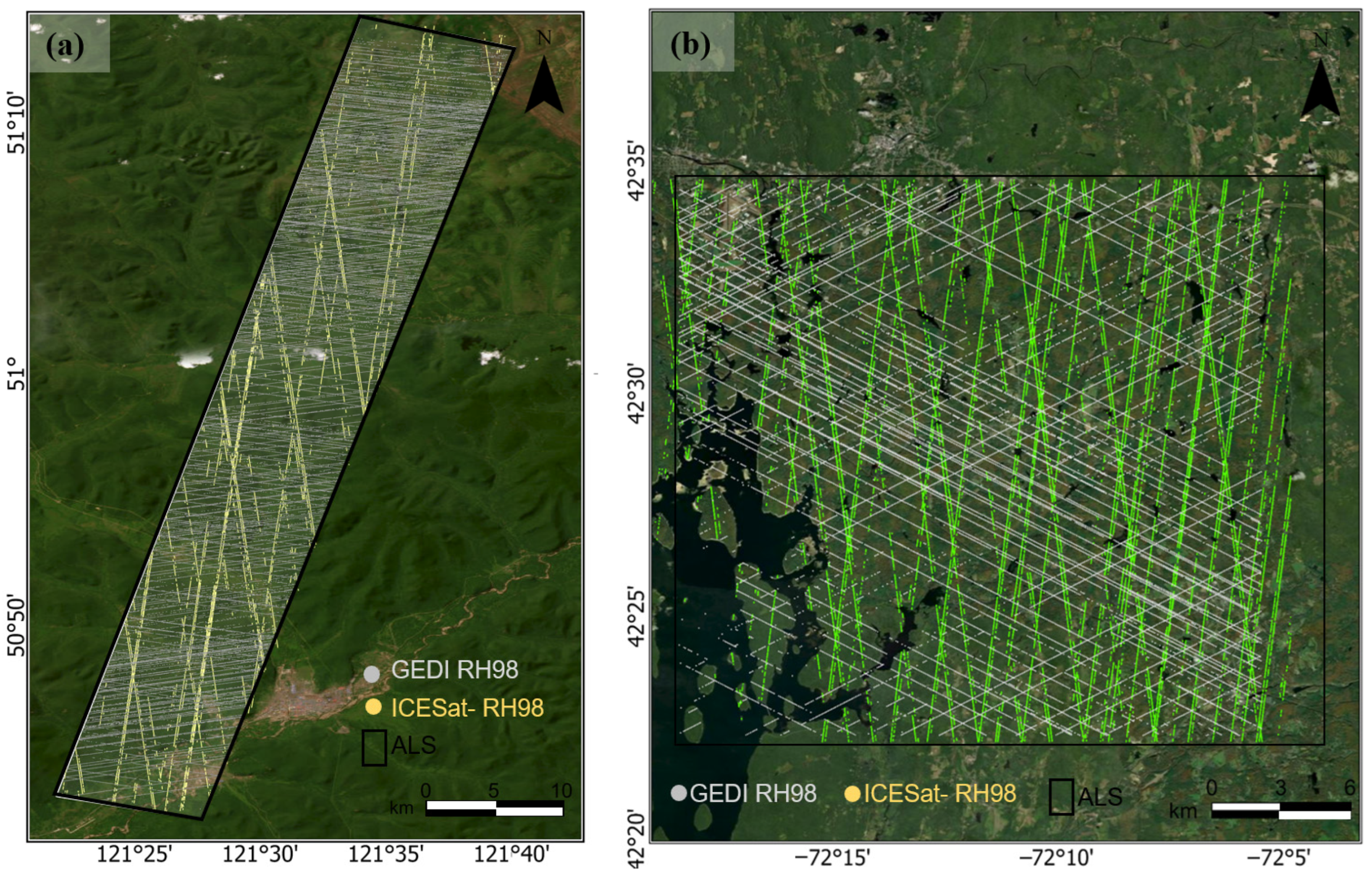
To comprehensively evaluate the applicability of the proposed refinement strategy for spaceborne LiDAR forest height reference points under different forest structures and topographic conditions, two representative study areas were selected: the Genhe study area in China and the HARV study area in the United States. These two regions represent typical forest ecosystems across different latitudinal zones. The geographical locations of the study areas, the spatial distribution of spaceborne LiDAR footprints, and the coverage of ALS validation data are shown in Figure 1. The black rectangular boxes in the figure indicate the actual spatial boundaries of the high-resolution ALS data used for accuracy validation, while the dense point trajectories distributed within and around the boxes represent the initial GEDI and ICESat-2 forest height retrievals extracted in this study.

Figure 1. Locations of the study areas and coverage of the ALS validation data (yellow boxes). (a) Genhe coniferous forest study area, China; (b) HARV mixed broadleaf forest study area, USA.

The Genhe study area is located in the Greater Khingan Mountains forest region in the northeastern part of the Inner Mongolia Autonomous Region, China (central coordinates: approximately 121.32°E, 51.01°N). The topography of this area is characterized primarily by undulating hills with relatively gentle terrain transitions. It is a typical boreal coniferous forest biome with a relatively high forest coverage (approximately 68%). The stand structure is relatively sparse and evenly distributed, with conifers as the dominant tree species. Based on field and airborne data statistics, the average forest height in this area is about 15 m, with most tree heights ranging from 5 to 20 m. The HARV study area is located in Massachusetts, USA (central coordinates: approximately 72.11°W, 42.26°N). The topography of this area features a mixed landscape of mountains and hills. It is a temperate mixed broadleaf forest biome with high forest coverage (approximately 76%) and a dense canopy layer. The HARV site features a complex canopy structure with generally taller trees. The average forest height in this area is approximately 25 m, with tree heights primarily distributed between 15 and 30 m.

2.2. Spaceborne LiDAR RH98 Data

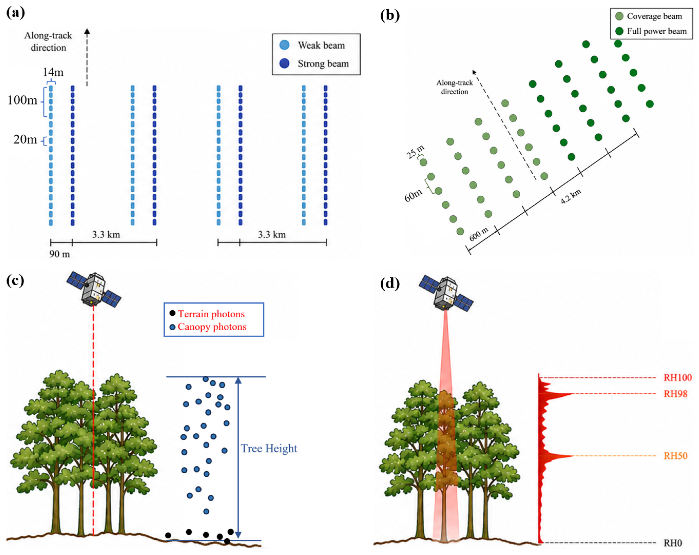
This study acquired forest canopy height data from two mainstream spaceborne LiDAR systems, ICESat-2 and GEDI. Their spatial sampling patterns and altimetry principles are illustrated in Figure 2 [10,13].

Figure 2. Schematic diagram of spatial sampling patterns and forest canopy height retrieval principles for spaceborne LiDAR. (a) ICESat-2 ground tracks and 20 m segments; (b) GEDI footprint distribution; (c) Principle of ICESat-2 photon-counting altimetry; (d) Principle of GEDI full-waveform relative height percentiles.

ICESat-2, launched in September 2018, carries the Advanced Topographic Laser Altimeter System (ATLAS), which utilizes photon-counting technology to acquire vertical structure information of the global Earth surface and vegetation (Figure 2c) [7]. This study utilized the newly released ATL08 (Version 7) land and vegetation height product [47]. Specifically, unlike the 100 m segment data commonly used in previous studies, this study extracted canopy height parameters at the 20 m segment scale (as shown in Figure 2a). The actual spatial resolution of this segment is approximately 14 m × 20 m. Compared to the 100 m segments, it provides greater data density and higher footprint resolution, enabling a more detailed characterization of local forest canopy variations. To minimize temporal discrepancies caused by vegetation growth or terrain changes, the selected ICESat-2 data were acquired during years close to those of the airborne LiDAR data, specifically 2023 to 2025 for the Genhe study area and 2021 to 2023 for the HARV study area. These footprints are shown as light gray dots in Figure 1.

GEDI is a full-waveform LiDAR system mounted on the International Space Station, designed specifically for the detailed observation of three-dimensional vegetation structures. It has been operating since its launch in December 2018 [10]. This study extracted the GEDI L2A elevation and height metrics product. The basic observation unit of this product is a circular footprint with a diameter of approximately 25 m, and its multi-beam ground coverage pattern is shown in Figure 2b. Regarding the height metric selection, the relative height at the 98th percentile of waveform energy (RH98, Figure 2d) was extracted as the representative value for estimating forest canopy height. For temporal window matching, the filtering conditions for GEDI data were consistent with those for ICESat-2, selecting observations from years close to the airborne reference data. Furthermore, to evaluate the proposed refinement strategy’s ability to recover low-quality data, daytime observations and weak or coverage beam data, which are typically discarded in conventional processing, were retained during the initial data preparation stage. These were combined with nighttime observations and strong or power beam data to form the initial set of reference points for refinement, with their footprints shown as green dots in Figure 1.

2.3. Airborne LiDAR Validation Data

To validate the accuracy of canopy heights retrieved from spaceborne LiDAR, high-precision airborne LiDAR data were acquired and used as the ground reference truth. The airborne LiDAR data for the Genhe study area were collected by a local flight mission in August 2024, covering an area of approximately 7 km × 60 km. Data for the HARV study area were obtained from the National Ecological Observatory Network (NEON) [48], utilizing high-density airborne LiDAR products collected in August 2022, with a coverage area of approximately 20 km × 15 km. The spatial coverage of the validation data for both study areas is indicated by the black rectangular boxes in Figure 1.

Based on the acquired initial airborne point cloud data, 1 m resolution canopy height models (CHMs) were generated for both study areas. To ensure spatial and metric consistency between the airborne validation data and the spaceborne LiDAR products, the effective observation areas of GEDI and ICESat-2 (i.e., the 25 m diameter circular footprints and the 14 m × 20 m rectangular segments) were used as reference boundaries. The high-resolution CHMs were spatially aggregated within these boundaries to calculate the airborne 98th percentile height (i.e., ALS RH98) [13].

2.4. Global CHM Products

To implement the proposed refinement strategy, it is necessary to introduce continuous forest height products with reasonable morphological characteristics as prior spatial envelope references. Therefore, several mainstream large-scale continuous CHM products trained and calibrated based on GEDI footprints were selected as auxiliary data. These primarily include:

(1)

Meta CHM [17]: A global canopy height map developed by Meta, using high-resolution commercial optical satellite imagery (Maxar, resampled to 1 m) as input, with features extracted by a self-supervised Vision Transformer (DINOv2) model. During the model training phase, this product used ALS raster data as the primary supervision signal to ensure high-resolution local prediction details. Subsequently, in the post-processing phase, a low-resolution regression network trained on GEDI RH95 was introduced to extract global scaling factors to calibrate the initial prediction map.

(2)

ETH CHM [15]: A 10 m resolution global tree height product developed by researchers at ETH Zurich generated based on single-date Sentinel-2 imagery using a deep probabilistic learning framework (CNN ensemble), calibrated with GEDI RH98 as control points.

(3)

Pauls CHM [16]: A 10 m resolution tree height product developed by Pauls et al., generated by fusing Sentinel-1 radar and Sentinel-2 spectral time-series features. It was trained using deep fully convolutional networks (e.g., U-Net) combined with GEDI RH100 and topographic filtering.

(4)

UMD CHM [25]: A 30 m resolution global tree height product developed by the University of Maryland (UMD), generated using Landsat time-series imagery as the primary feature input by University of Maryland (UMD), trained with traditional machine learning algorithms (Bagged Regression) combined with GEDI RH95.

A common characteristic of the aforementioned auxiliary products is that they all use GEDI observations as training samples for learning and prediction. Although they lack the absolute micro-level accuracy of airborne LiDAR at the single-point scale, they preserve the natural continuous growth characteristics of regional forest heights after spatial aggregation and model smoothing. This study utilizes the physical envelope provided by these products as a priori spatial knowledge to assist in the reliable identification and removal of gross errors and outliers in the initial spaceborne LiDAR observations.

3. Methodology

3.1. Initial Spaceborne LiDAR RH98 Retrievals

In the initial data preparation stage, to overcome the data sparsity limitation caused by traditional studies that retain only nighttime and strong beam data, this study extracted all available spaceborne LiDAR observations covering both daytime and nighttime, as well as strong and weak beams (power and coverage beams). For GEDI observations, this study utilized the L2A elevation and relative height product, extracting the relative height at the 98th percentile of waveform energy (RH98) as the observed tree height. At this stage, only basic quality control was applied to exclude completely invalid observations, requiring a valid quality flag (quality_flag = 1), no degradation record (degrade_flag = 0), and a waveform sensitivity greater than 0.90 (sensitivity > 0.90).

For ICESat-2 data, the Version 7 (V007) ATL08 Land and Vegetation Height product was used to extract the canopy height parameter (h_canopy, representing the 98th percentile of the relative canopy photon heights) at a 20 m spatial segment scale as the observed forest height [47]. The basic filtering conditions were set to require a total number of photons within the segment greater than 50 (n_seg_ph > 50), a number of valid canopy photons greater than 10 (n_ca_photons > 10), and low atmospheric cloud interference (cloud_flag_atm ≤ 2) [13,41]. Through preliminary filtering with these relaxed conditions, this study retained an initial reference point set with the maximum possible density.

3.2. Refinement Strategy Assisted by a Priori CHM Products

Relaxing the initial filtering conditions inevitably introduces extreme gross errors caused by factors such as solar background noise, multipath scattering, and complex terrain. To effectively identify and eliminate these noise points from the massive initial dataset, this study proposes an adaptive refinement strategy assisted by an a priori continuous CHM product. The core of this strategy lies in utilizing a large-scale continuous CHM with a morphologically reasonable spatial structure as a prior spatial envelope, thereby providing a soft constraint for the spaceborne observations.

In practical implementation, this study introduced four mainstream global forest height products (Meta 1 m, ETH 10 m, Pauls 10 m, and UMD 30 m) as candidate auxiliary data sources. By systematically comparing their performance in characterizing the natural continuous distribution of forest heights and the degree of numerical dispersion, the product that exhibited a compact core scatter density, lacked obvious numerical discontinuities, and best aligned with the actual vertical growth space of the forest was selected as the final macroscopic a priori envelope (denoted as $H_{prior}$).

Regarding the specific algorithm design for refinement, this strategy does not rely on local airborne data for supervised training; rather, it achieves the adaptive exclusion of gross errors based on statistical characteristics.

First, the corresponding tree height value $H_{prior}$ is extracted for each spaceborne LiDAR footprint using scale-matching strategies. For the 30 m UMD CHM, a point-to-point matching at the footprint center is applied. For the 10 m Pauls and ETH CHMs (which are already smoothed during generation), a local window average (a 3 × 3 pixel window for GEDI and a 2 × 2 window for ICESat-2) is computed to minimize spatial errors. For the 1 m Meta CHM, the 98th percentile (P98) of the pixels within each footprint is extracted, consistent with the validation method used in the original Meta CHM study. Subsequently, the relative height difference $\Delta h_i$ between the initial spaceborne observation ($H_{spaceborne,i}$) and $H_{prior,i}$ is calculated:

$$\Delta h_i=H_{spaceborne,i}-H_{prior,i}$$

(1)

Within a local region, the deviations of true and valid tree heights generally follow an approximate normal distribution, whereas large error points and ground-penetrating noise caused by cloud obscuration or strong sunlight appear as extreme values far from the center of the distribution. To prevent these heavy tails from inflating the fitted standard deviation, a preliminary physical filter is applied prior to the Gaussian parameter estimation, whereby any absolute height difference $\left|\Delta h_i\right|$ exceeding the average forest height (e.g., exceeding 15 m in Genhe) is excluded prior to the Gaussian fitting. Therefore, the mean (${\mu }_{\Delta h}$) and standard deviation (${\sigma }_{\Delta h}$) of the height difference sequence within the local region are calculated:

$${\mu }_{∆h}={\displaystyle \frac{{\sum }_{i=1}^N{∆h}_i}{N}}$$

(2)

$${\sigma }_{∆h}=\sqrt{{\displaystyle \frac{{\sum }_{i=1}^N({∆h}_i-\mu ∆h{)}^2}{N}}}$$

(3)

Finally, one standard deviation ($1\sigma$) is set as the adaptive truncation threshold to construct the valid reference point set (denoted as $S_{valid}$). Specifically, only the observations with relative height differences falling within this dynamic interval are retained:

$$S_{valid}=\left\{H_{spaceborne,i}\right|\left|∆h_i-\mu ∆h\right|\le {\sigma }_{\Delta h}\}$$

(4)

This soft constraint mechanism, which integrates statistical metrics with a prior spatial envelope, can effectively isolate extreme outliers without altering the initial physical observation attributes of the spaceborne data. Specifically, the Gaussian parameters (${\mu }_{\Delta \mathrm{h}}$ and ${\sigma }_{\Delta \mathrm{h}}$) are computed independently for GEDI and ICESat-2 datasets, ensuring that the 1$\sigma$ threshold dynamically adapts to each sensor’s unique noise and footprint characteristics. Consequently, it achieves high-quality refinement for high-density reference points. Although a $1\sigma$ truncation threshold is relatively strict, it perfectly aligns with the primary objective of this study—extracting high-accuracy RH98. Furthermore, since relaxing the initial filtering conditions (e.g., retaining all daytime and weak/coverage beam) provides a massive initial sample base, applying the $1\sigma$ threshold guarantees strict accuracy while still retaining more high-quality reference points than traditional filtering methods.

3.3. Accuracy Assessment

In the accuracy validation phase, considering the spatial scale differences between the discrete spaceborne LiDAR footprints and the continuous ALS grids, a spatial buffer statistical method was employed to extract the validation reference. Specifically, a circular buffer with a diameter of 25 m was constructed using the center of the GEDI footprint, and a 14 m × 20 m rectangular buffer was constructed using the center of the ICESat-2 segment. Subsequently, the tree height distribution of ALS CHM pixels within the corresponding buffer was calculated, and the 98th percentile height (ALS RH98) was extracted as the relative reference truth. This process ensures the rigor of spatial matching. Importantly, the validation reference dataset (ALS RH98) remained completely independent throughout the study; it was never utilized in the external CHM selection or the unsupervised filtering process. This absolute separation prevents any circular validation or self-evaluation bias, ensuring an objective accuracy assessment.

To quantitatively evaluate the quality and algorithm performance before and after refinement, this study selected four statistical metrics: the coefficient of determination ($R^2$), root mean square error (RMSE), bias ($Bias$), and relative RMSE ($rRMSE$):

$$R^2=1-{\displaystyle \frac{{\sum }_{i=1}^N(x_i-y_i{)}^2}{{\sum }_{i=1}^N(y_i-{\overline{y}}_i{)}^2}}$$

(5)

$$RMSE=\sqrt{{\displaystyle \frac{{\sum }_{i=1}^N(x_i-y_i{)}^2}{N}}}$$

(6)

$$rRMSE={\displaystyle \frac{RMSE}{\overline{y}}}\times 100\%$$

(7)

$$Bias={\displaystyle \frac{{\sum }_{i=1}^N\left(x_i-y_i\right)}{N}}$$

(8)

where $N$ represents the total number of successfully matched valid footprint samples, $x_i$ represents the spaceborne LiDAR tree height observation after processing strategies, $y_i$ is the ALS RH98 relative truth obtained based on spatial buffer statistics, and $\overline{y}$ is the average of all airborne validation truth values.

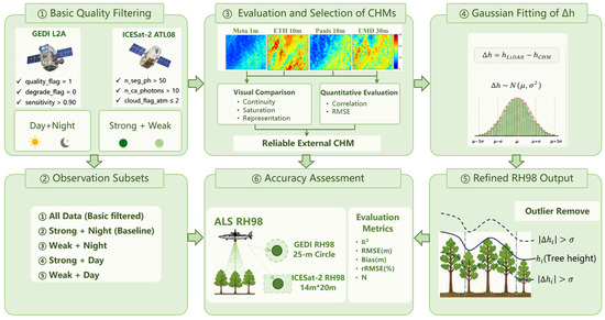
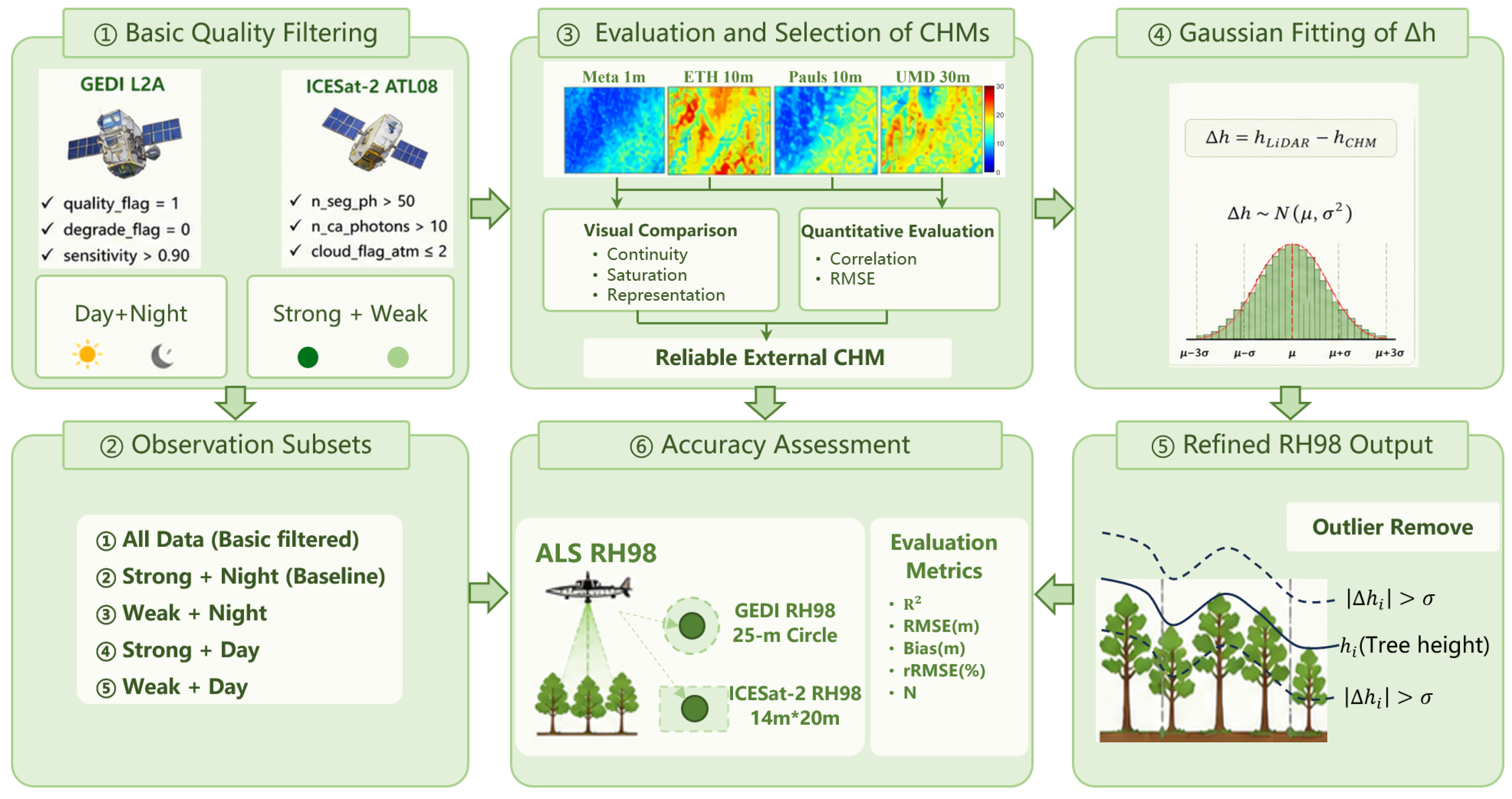
Overall, the flowchart of the proposed method is illustrated in Figure 3. First, based on relaxing the quality filtering conditions to maximize the retention of initial spaceborne RH98, the data are divided into observation subsets covering different beams and time periods to provide a baseline for comparisons. In the main refinement process, a comprehensive visual and quantitative evaluation is initially conducted to select the global CHM products with the reasonable morphology as the prior spatial envelope. Subsequently, the relative height differences between the initial spaceborne RH98 and the selected auxiliary CHM are calculated and subjected to Gaussian fitting. The resulting dynamic truncation interval is used to adaptively remove outliers that deviate significantly from the true canopy. Finally, the refined high-density observations and the initial subsets are uniformly input into the accuracy assessment module. Based on the spatial buffer statistical results of the high-precision ALS data, the practical performance of the refinement strategy under various observation scenarios is comprehensively validated.

Figure 3. Overall flowchart of the spaceborne LiDAR forest height reference point refinement strategy assisted by a priori continuous CHM.

4. Results

4.1. Accuracy of Initial Spaceborne RH98

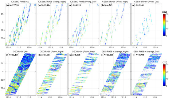
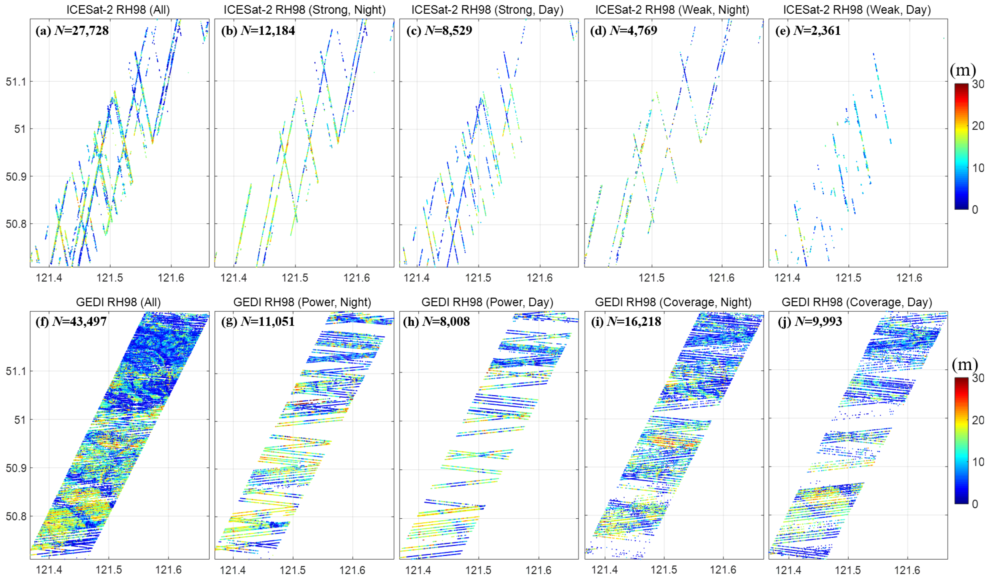
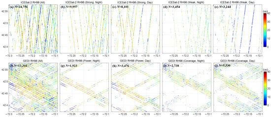
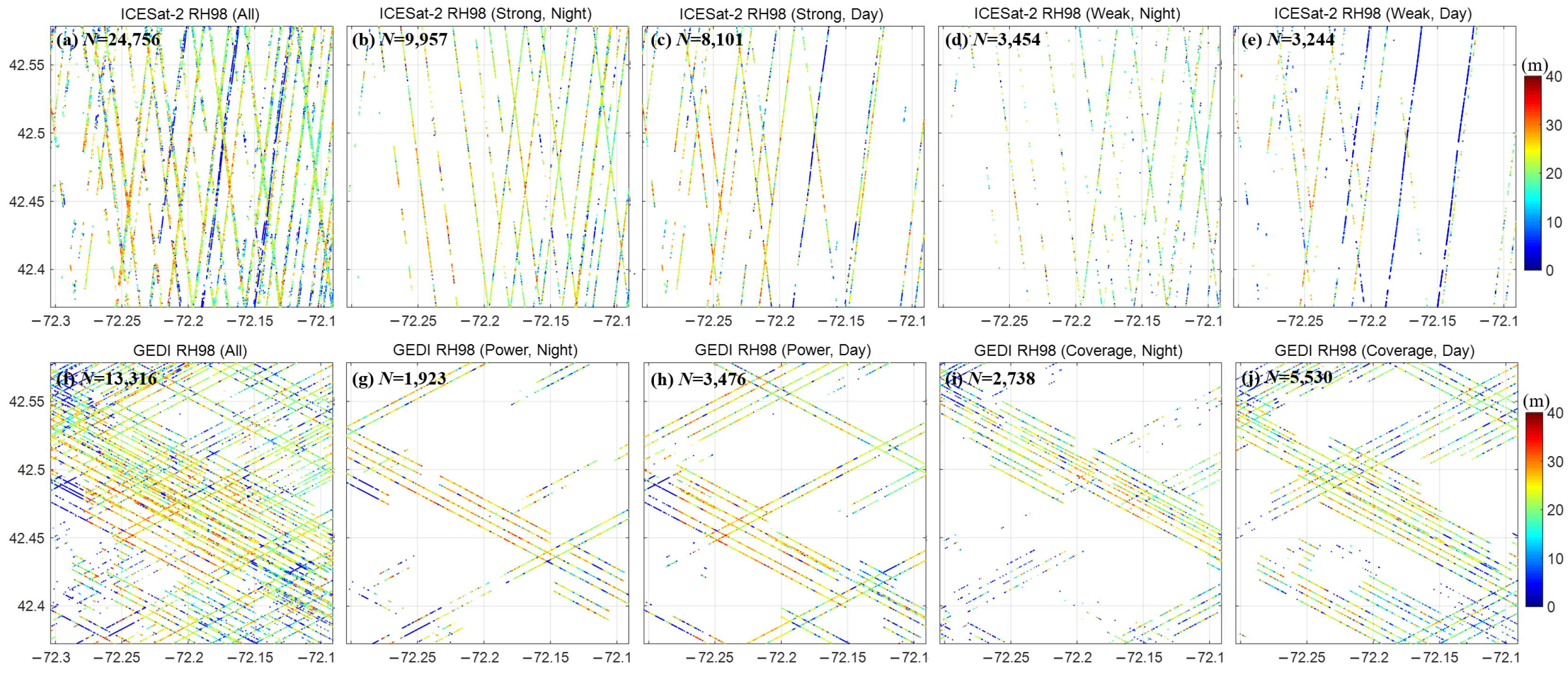
Figure 4 and Figure 5 illustrate the spatial distribution and the number of valid footprints (N) of spaceborne LiDAR under different filtering conditions in the Genhe and HARV study areas. When retaining all observations regardless of acquisition time and beam type (Figure 4a,f and Figure 5a,f), both study areas obtain relatively dense spatial coverage. However, when applying the traditional strict filtering strategy, which retains only nighttime strong or power beam observations, the number of valid footprints decreases substantially. Specifically, in the Genhe study area, the number of valid footprints for ICESat-2 (Figure 4b) and GEDI (Figure 4g) decreased from 27,728 and 43,497 to 12,184 and 11,051, respectively. In the HARV study area, which features taller and denser vegetation, the number of valid ICESat-2 footprints (Figure 5b) dropped to 9957, and GEDI footprints (Figure 5g) decreased from 13,316 to 1923, resulting in an 85% data loss. This indicates that while strict filtering helps ensure data quality, it directly causes the spatial distribution of reference points to become sparse.

Figure 4. Footprint distribution of spaceborne RH98 in the Genhe study area. (a–e) ICESat-2; (f–j) GEDI. The subplots show the entire observation set and its subsets categorized by night/day and strong/weak (power/coverage) beams. N indicates the number of footprints.

Figure 5. Footprint distribution of spaceborne RH98 in the HARV study area. (a–e) ICESat-2; (f–j) GEDI. The subplots show the entire observation set and its subsets categorized by night/day and strong/weak (power/coverage) beams.

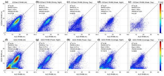
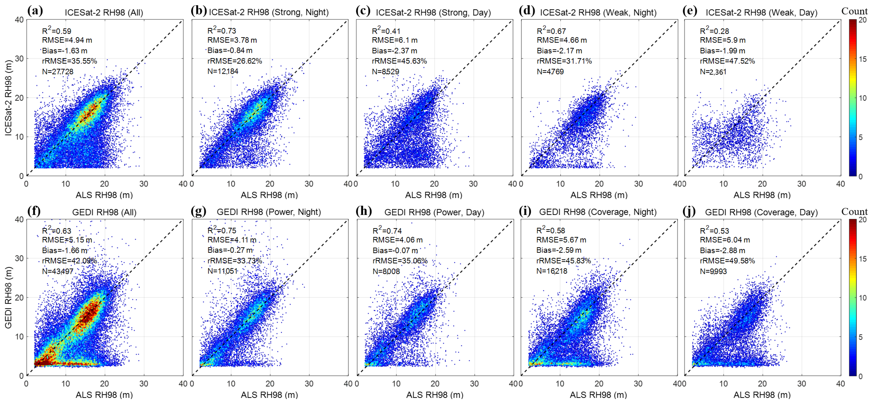
Figure 6 illustrates the accuracy comparison between the initial spaceborne LiDAR RH98 and the ALS truth values in the Genhe study area. For all available data covering beam types and time periods (Figure 6a,f), a certain number of outliers are present in the scatter plots, with the RMSEs for ICESat-2 and GEDI being 4.94 m and 5.15 m, respectively. In contrast, for the subset of nighttime strong (power) beam data retained after strict filtering (Figure 6b,g), the scatter distribution concentrates more closely around the $y=x$ line. The RMSEs decrease to 3.78 m and 4.11 m, and the $R^2$ remains above 0.73, indicating an effective improvement in data accuracy. However, for GEDI, the RMSE of nighttime power beam observations is 4.11 m, which performs slightly worse than the daytime power beam observations (RMSE = 4.06 m). Furthermore, independent observation of the weak and coverage beam data (Figure 6d,e,i,j) reveals that due to their lower pulse emission energy, their signal penetration capability is limited. Consequently, these data are more prone to noise and exhibit a tendency to underestimate the actual tree heights for some RH98 footprints.

Figure 6. Accuracy validation scatter plots of initial spaceborne LiDAR RH98 in the Genhe study area. (a–e) ICESat-2 observation subsets; (f–j) GEDI observation subsets. The columns, from left to right, display the results for: all data, strong (power) beams at night, strong (power) beams during the day, weak (coverage) beams at night, and weak (coverage) beams during the day.

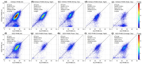
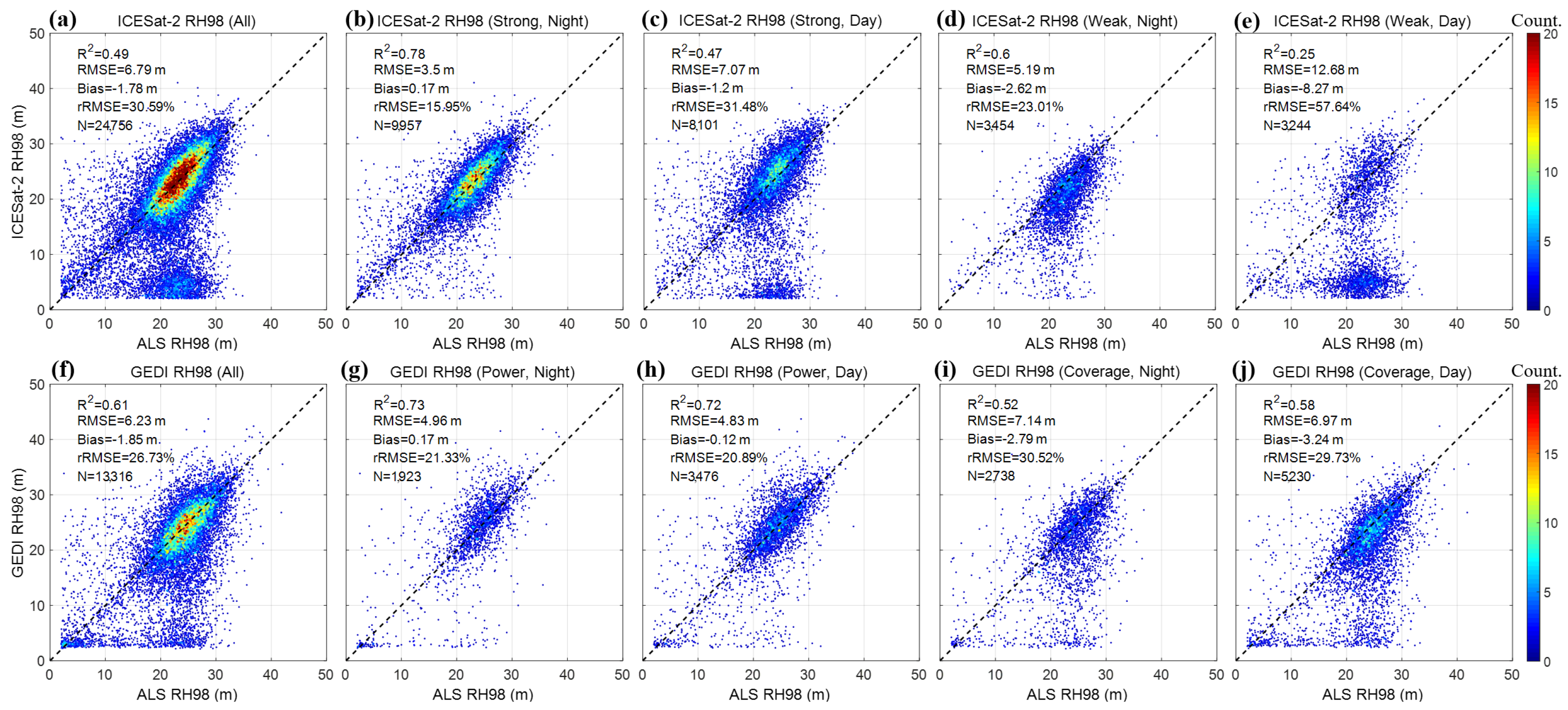
Figure 7 presents the accuracy validation results for the HARV study area. Due to the taller and denser forest canopy in this region, the RMSEs of ICESat-2 and GEDI reach 6.79 m and 6.23 m, respectively (Figure 7a,f). Regarding the performance across different subsets, the advantage of the nighttime strong (power) beam combination exhibits systematic differences between the two sensors. For ICESat-2, the nighttime strong beam combination represents the optimal observation condition (Figure 7b), with its RMSE decreasing to 3.5 m. However, for GEDI, the accuracy of the nighttime power beam observations (Figure 7g, RMSE = 4.96 m) does not outperform that of the daytime power beam observations (Figure 7h, RMSE = 4.83 m). Concurrently, the signal attenuation of weak beam data is more pronounced in dense forest areas. For instance, the daytime weak beam observations from ICESat-2 (Figure 7e) display a significant underestimation (Bias = −8.27 m), with an RMSE reaching 12.68 m. Because daytime and weak beam data are more likely to contain gross errors caused by cloud cover and solar background noise, conventional processing workflows typically discard them entirely.

Figure 7. Accuracy validation scatter plots of initial spaceborne LiDAR RH98 in the HARV study area. (a–e) ICESat-2 observation subsets; (f–j) GEDI observation subsets. The columns, from left to right, display the results for: all data, strong (power) beams at night, strong (power) beams during the day, weak (coverage) beams at night, and weak (coverage) beams during the day.

4.2. Correlation Analysis Between Global CHM Products and Spaceborne RH98

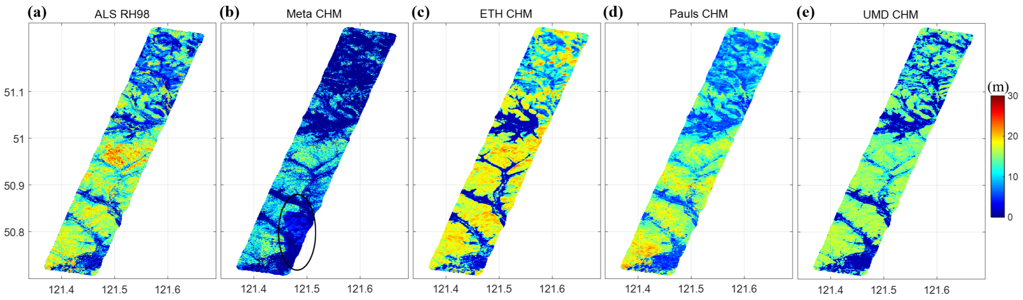
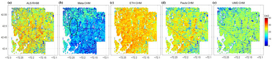
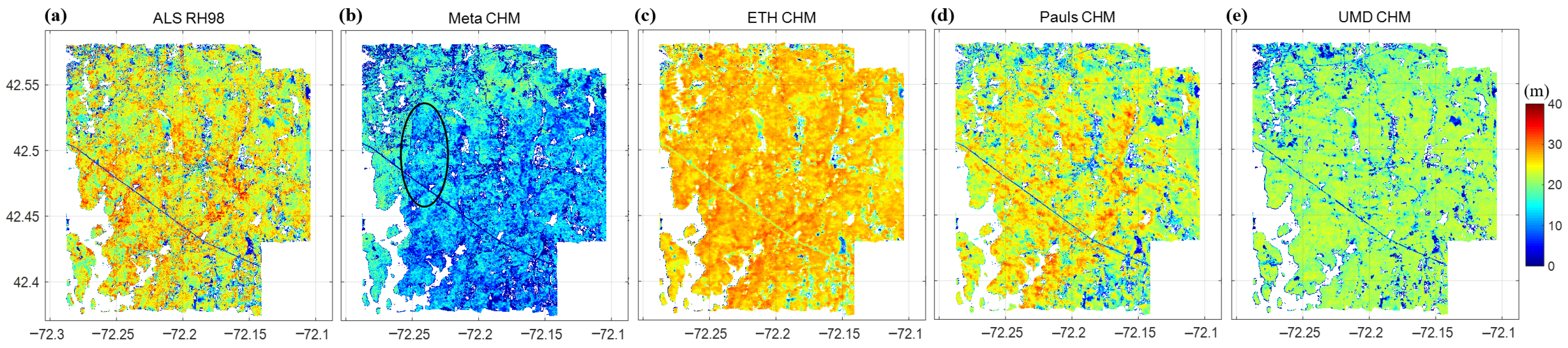
To validate and select the optimal prior spatial envelope, this study conducted a qualitative spatial visualization comparison between the extracted ALS RH98 and four mainstream global continuous forest height products (Meta 1 m, ETH 10 m, Pauls 10 m, and UMD 30 m). Figure 8 and Figure 9 display the visualization results of these products in the Genhe and HARV study areas, respectively.

Figure 8. Spatial visual comparison of ALS truth and various global CHM products in the Genhe study area. (a) The 1 m resolution ALS RH98; (b) Meta CHM 1 m; (c) ETH CHM 10 m; (d) Pauls CHM 10 m; (e) UMD CHM 30 m.

Figure 9. Spatial visual comparison of ALS truth and various global CHM products in the HARV study area. (a) The 1 m resolution ALS RH98; (b) Meta CHM 1 m; (c) ETH CHM 10 m; (d) Pauls CHM 10 m; (e) UMD CHM 30 m.

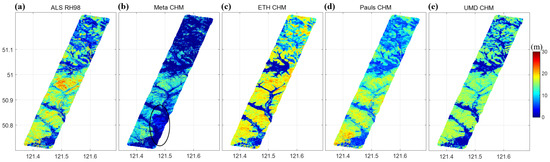
By comparing them with the ALS RH98, distinct differences in spatial continuity and height reconstruction capabilities can be observed among the products. Limited by the quality of optical imagery, the Meta product exhibits noticeable data gaps and discontinuities in local areas (as indicated by the circled regions in Figure 8b and Figure 9b). Furthermore, because its training data are derived from ALS CHMs, its overall height estimation tends to be systematically underestimated. Although the UMD CHM shows reasonable spatial continuity, it struggles to differentiate varying forest heights, presenting generally overestimated and highly saturated visual features in taller tree regions and failing to reflect the fine-scale undulations of the forest canopy. The performance of the ETH 10 m product falls between the two, still exhibiting some degree of overestimation and saturation for tall trees. In contrast, the Pauls 10 m product demonstrates relatively reasonable morphological characteristics in both study areas. It not only effectively avoids extreme saturation and substantial underestimation but also visually aligns most closely with the spatial distribution of the ALS truth in delineating canopy boundaries and height undulation trends.

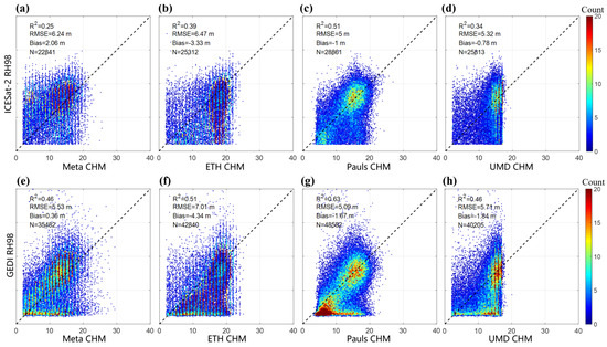
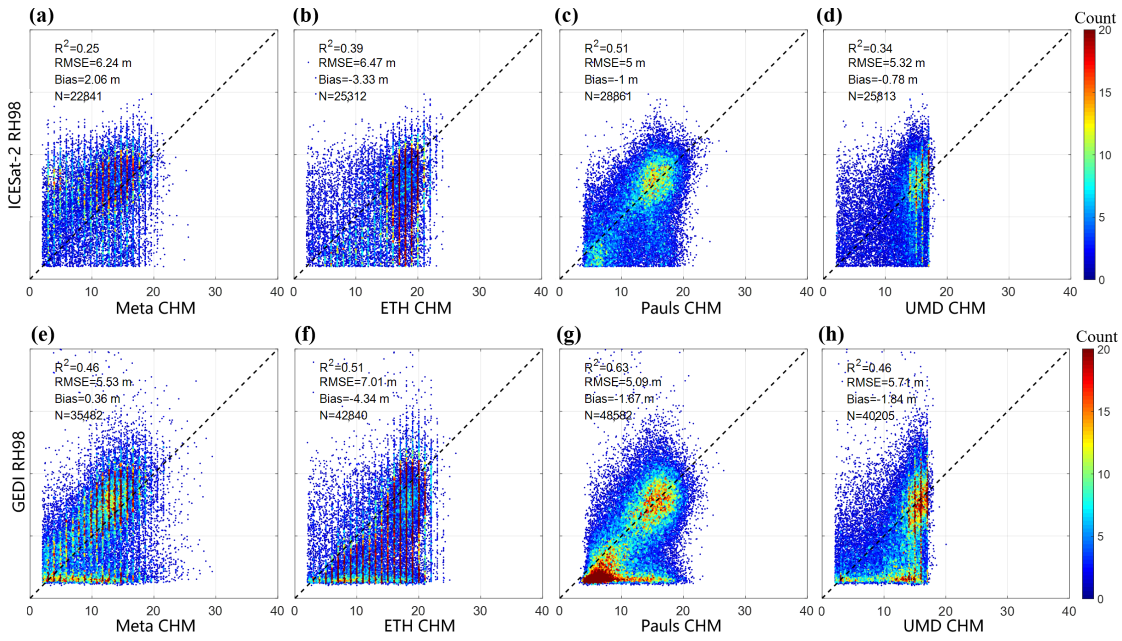
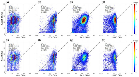
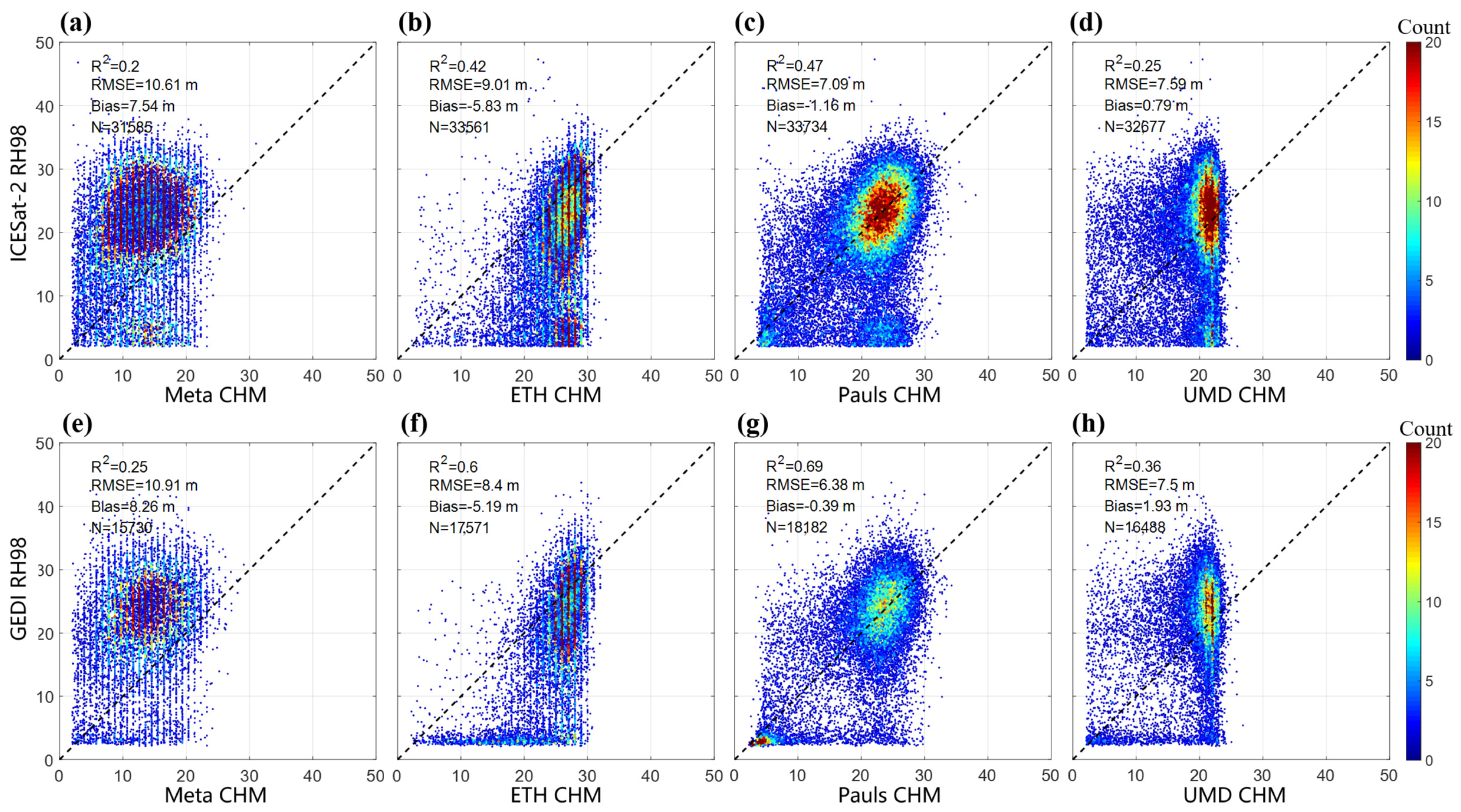
Following the qualitative evaluation of spatial visualization, this study further conducted a quantitative scatter plot analysis between the four global CHM products and all available spaceborne LiDAR RH98 footprints (i.e., all data retained after quality parameter filtering) to verify the reliability of each product as a physical envelope. Figure 10 and Figure 11 present the quantitative comparison results in the Genhe and HARV study areas, respectively. Judging from the scatter distribution characteristics and statistical metrics, the different products exhibit significant variations in characterizing natural forest heights. The Meta CHM (Figure 10a and Figure 11a) shows substantial tree height underestimation in both study areas. For instance, in the HARV study area with taller forest, its biases relative to ICESat-2 and GEDI reach 7.54 m and 8.26 m, respectively. The scatter points broadly deviate below the $y=x$ line, failing to provide an effective tall-tree envelope constraint. The $R^2$ of the ETH CHM (Figure 10b and Figure 11b) improves; however, due to the algorithmic limitations in mapping image features, noticeable numerical discontinuities appear in the scatter plots, along with a certain underestimation tendency, making it difficult to reflect the continuous variation of actual tree heights. The UMD 30 m CHM product exhibits pronounced saturation in tall tree regions above 15–22 m, where scatter points form a saturation wall at a specific value on the horizontal axis, losing the ability to capture canopy height variations.

Figure 10. Quantitative scatter plots of initial full-set spaceborne RH98 observations versus various global CHM products in the Genhe study area. ICESat-2 versus: (a) Meta CHM; (b) ETH CHM; (c) Pauls CHM; (d) UMD CHM. GEDI versus: (e) Meta CHM; (f) ETH CHM; (g) Pauls CHM; (h) UMD CHM.

Figure 11. Quantitative scatter plots of initial full-set spaceborne RH98 observations versus various global CHM products in the HARV study area. (a) Meta CHM; (b) ETH CHM; (c) Pauls CHM; (d) UMD CHM. GEDI versus: (e) Meta CHM; (f) ETH CHM; (g) Pauls CHM; (h) UMD CHM.

In contrast, the Pauls 10 m CHM product (Figure 10c and Figure 11c) exhibits the best quantitative performance. Its core scatter density presents a compact and continuous elliptical distribution, symmetrically aligned along the $y=x$ line. In the Genhe study area, the Pauls CHM achieves the highest correlation with ICESat-2 and GEDI ($R^2$ of 0.51 and 0.63, respectively) and the smallest errors (RMSE of 5 m and 5.09 m, respectively). In the HARV study area, this product similarly maintains the optimal statistical performance and effectively avoids issues such as pronounced saturation and significant underestimation.

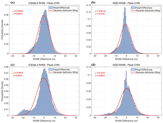
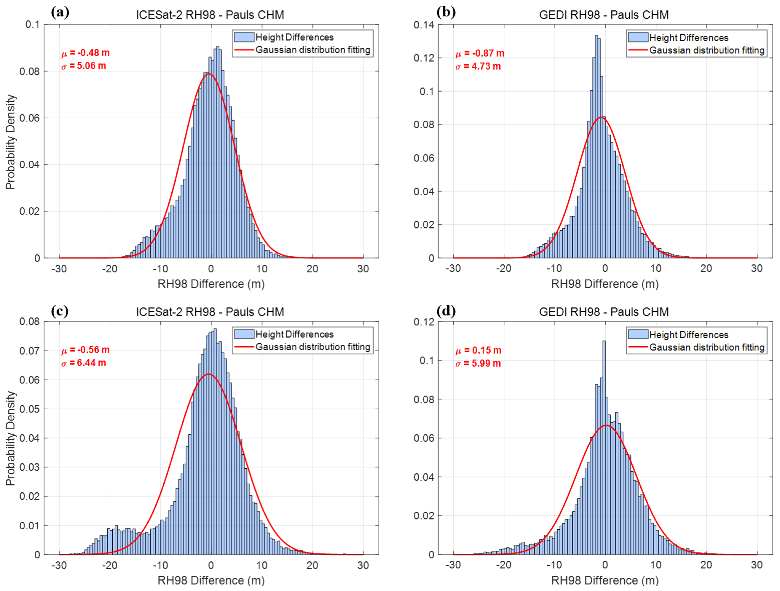
The combination of visual analysis and quantitative results confirms that the Pauls CHM can relatively accurately reflect the natural continuous envelope morphology of regional forests. Therefore, it was selected as the reliable a priori data in this study. To further verify the feasibility of using this auxiliary data to remove gross errors, this study calculated the relative height differences ($\Delta h$) between all available initial spaceborne LiDAR observations and the Pauls CHM, and plotted their probability density distributions. As shown in Figure 12, the blue bars represent the distribution of the differences, and the red line indicates the fitted normal distribution curve, while μ and σ denote the mean and standard deviation of the distribution, respectively. In both the Genhe and HARV study areas, and for both ICESat-2 and GEDI, the actual distributions of height differences (blue histograms) closely align with the fitted normal distribution curves (red solid lines). The height difference data are densely concentrated around the mean ($\mu$) with a small overall bias, indicating that the primary trend of the spaceborne observations is fundamentally consistent with the physical envelope of the Pauls CHM. Meanwhile, the histograms exhibit varying degrees of tailing on both sides. These extreme values deviating from the center represent the outliers mixed within the daytime and weak beam data. This result visually corroborates the algorithmic hypothesis that “the deviations of valid tree heights approximately follow a normal distribution, while gross errors are distributed in the tails. Therefore, using the Pauls CHM as a reference and selecting the $1\sigma$ interval of the normal distribution as the threshold to exclude outliers is supported by ample data and theoretical rationale.

Figure 12. Probability density histograms of the relative height difference ($\Delta h$) between the initial full-set spaceborne RH98 and Pauls CHM in the two study areas. (a) ICESat-2 in Genhe; (b) GEDI in Genhe; (c) ICESat-2 in HARV; (d) GEDI in HARV.

4.3. Accuracy Validation After Refinement

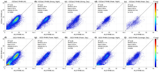
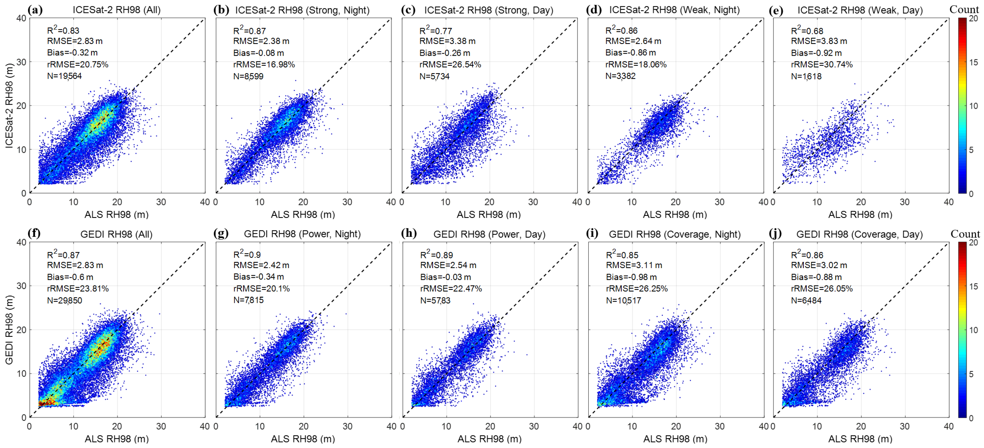
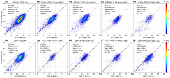
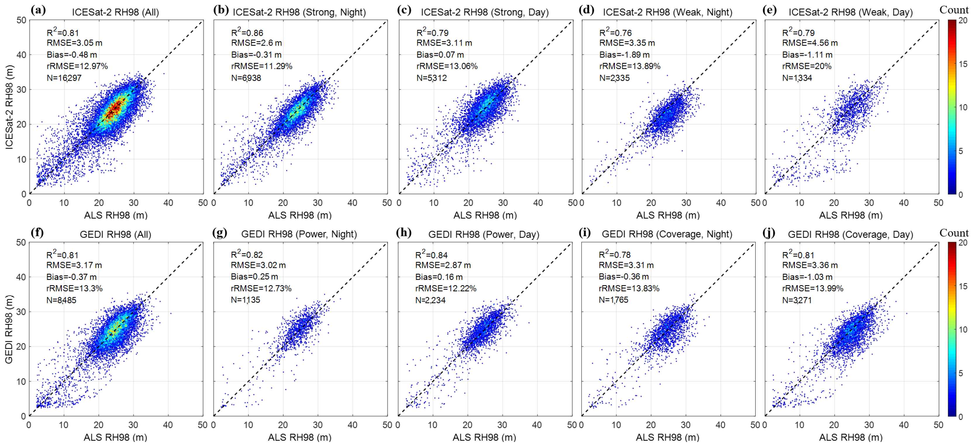
After applying the $1\sigma$ adaptive truncation strategy based on the Pauls CHM, this study re-evaluated the accuracy of the spaceborne LiDAR data using the ALS data. Figure 13 and Figure 14 present the scatter distributions and statistical metrics after refinement in the Genhe and HARV study areas, respectively. Compared to the scattered state containing numerous outliers before refinement, the refined spaceborne data scatter points converge closely around the $y=x$ line, indicating an effective improvement in overall data quality.

Figure 13. Accuracy validation scatter plots of spaceborne LiDAR RH98 after the refinement in the Genhe study area. (a–e) Validation of the refined ICESat-2 RH98; (f–j) Validation of the refined GEDI RH98.

Figure 14. Accuracy validation scatter plots of spaceborne LiDAR RH98 after the refinement in the HARV study area. (a–e) Validation of the refined ICESat-2 RH98; (f–j) Validation of the refined GEDI RH98.

First, in terms of overall accuracy, the refinement algorithm demonstrates a stable error control capability. Using the unfiltered initial all-available data as a baseline, in the Genhe study area, the overall RMSEs of ICESat-2 and GEDI decreased from their initial values of 4.94 m and 5.15 m to 2.83 m (the rRMSE decreased from 35.55% and 42.09% to 20.75% and 23.81%), representing accuracy improvements of 42.7% and 45.0%, with the overall $R^2$ values for both increasing to above 0.83. In the HARV study area, which features more complex terrain and forest canopies, the optimization effect is similarly evident. The overall RMSEs of ICESat-2 and GEDI decreased from 6.79 m and 6.23 m to 3.05 m and 3.17 m (the rRMSE decreased from 30.59% and 26.73% to 12.97% and 13.3%), corresponding to accuracy improvements of 55.1% and 49.1%, respectively, and $R^2$ values both reaching 0.81. Furthermore, this refined accuracy level even surpasses the strict traditional filtering results that retain only “nighttime + strong/power beam” data. Compared to the high-quality observation subsets obtained through traditional filtering, the proposed refinement strategy further reduces the overall RMSE by 12.6% to 36.0%, while avoiding substantial data loss. This effectively demonstrates the validity of the prior spatial envelope in adaptively filtering extreme gross errors.

Additionally, the proposed refinement strategy resolves the limitation of traditional methods that sacrifice data volume for fidelity. By comparing the number of valid reference points ($N$), it can be observed that while maintaining the overall data RMSE at a high-accuracy level of approximately 3 m, the data density retained after refinement is 1.5 to 4.4 times that of traditional strict filtering (which retains only nighttime strong/power beams). For example, in the Genhe study area, the numbers of valid points for ICESat-2 and GEDI after refinement are 19,564 and 29,850, respectively (compared to only 12,184 and 11,051 under traditional filtering). In the HARV study area, the number of valid GEDI footprints after refinement reaches 8485, which is considerably higher than the 1923 footprints remaining after traditional filtering.

Furthermore, this study demonstrates that weak/coverage beams and daytime observations, which are typically discarded in conventional practices, possess considerable potential for reuse. After refinement, the accuracy of these previously lower-quality subsets improves notably. Taking the HARV study area as an example, the ICESat-2 daytime weak beam data (Figure 14e), which initially exhibited the lowest accuracy with an RMSE of 12.68 m, show a reduced RMSE of 4.56 m after refinement, effectively eliminating the severe underestimation bias. For GEDI, the daytime coverage beam data (Figure 14j) achieve an RMSE of 3.36 m after refinement. This accuracy is comparable to that of nighttime observations and meets or exceeds the accuracy requirements of most existing large-scale mapping efforts. These results indicate that applying a reasonable a priori envelope as a soft constraint not only ensures the high accuracy of the final output reference points but also effectively recovers the application value of massive low SNR data. Consequently, this approach provides high-spatial-density control points for large-scale forest structure mapping.

5. Discussion

5.1. Performance Across Different Forest Heights and Terrain Slopes

Tree height and terrain slope are the primary physical factors contributing to systematic errors in spaceborne LiDAR observations. To further verify the robustness of the refinement strategy, this study conducted a segmented statistical analysis of the spaceborne LiDAR observations before and after optimization, using ALS tree heights and DTM slopes as references, and the accuracy metrics are listed in Table 1 and Table 2. Additionally, 95% confidence intervals (CIs) are reported alongside the overall Bias and RMSE metrics in both tables to quantify the statistical precision of the accuracy assessment.

Table 1. Accuracy metrics across different tree height segments before and after refinement.

Study Area	Sensor	ALS RH98	Before Refinement			After Refinement
			N	RMSE (m)	Bias (m)	N	RMSE (m)	Bias (m)
Genhe	ICESat-2	Total	27,728	4.94 ± 0.04	−1.63 ± 0.06	19,564	2.83 ± 0.03	−0.32 ± 0.04
		<10 m	6232	3.73	0.79	4818	2.75	0.56
		10–15 m	9274	4.14	−1.13	6609	2.72	−0.04
		15–20 m	10,771	5.31	−2.30	7419	2.81	−0.83
		20–25 m	1379	7.74	−4.63	687	5.16	−3.65
		>25 m	72	11.45	−8.88	31	9.21	−7.68
	GEDI	Total	43,497	5.15 ± 0.03	−1.66 ± 0.05	29,850	2.83 ± 0.02	−0.60 ± 0.03
		<10 m	14,897	3.39	−0.03	11,972	2.46	0.02
		10–15 m	13,030	5.17	−2.19	8139	3.15	−0.79
		15–20 m	13,869	5.94	−2.44	9009	2.90	−1.05
		20–25 m	1629	9.21	−5.41	708	5.42	−3.96
		>25 m	72	11.72	−9.32	22	9.87	−8.24
HARV	ICESat-2	Total	24,756	6.79 ± 0.06	−1.78 ± 0.08	16,297	3.05 ± 0.03	−0.48 ± 0.05
		<10 m	870	7.32	3.58	500	4.73	2.11
		10–15 m	946	6.05	0.52	487	4.49	0.60
		15–20 m	2968	5.97	−1.47	1764	3.64	0.27
		20–25 m	11,295	6.74	−2.71	7955	2.81	−0.55
		25–30 m	7703	7.72	−3.38	5127	3.17	−1.51
		>30 m	974	8.26	−4.04	464	5.11	−3.52
	GEDI	Total	13,316	6.23 ± 0.08	−1.85 ± 0.10	8485	3.17 ± 0.05	−0.37 ± 0.07
		<10 m	502	8.74	4.38	319	7.00	2.72
		10–15 m	444	7.32	2.00	231	6.16	1.75
		15–20 m	1521	5.75	0.18	908	4.11	1.31
		20–25 m	6185	5.79	−1.16	4041	3.03	0.09
		25–30 m	4046	6.36	−2.30	2689	3.25	−1.32
		>30 m	618	6.84	−3.27	297	5.12	−3.76

Table 2. Accuracy metrics across different terrain slope segments before and after refinement.

Study Area	Sensor	Slope	Before Refinement			After Refinement
			N	RMSE (m)	Bias (m)	N	RMSE (m)	Bias (m)
Genhe	ICESat-2	Total	27,728	4.94	−1.63	19,564	2.83	−0.32
		0–5°	12,758	4.56	−0.84	9124	2.85	−0.12
		5–10°	9317	4.97	−1.63	6555	2.89	−0.39
		10–15°	3282	5.15	−2.13	2228	2.92	−0.68
		15–20°	1354	5.16	−2.25	942	3.28	−1.00
		>20°	1017	4.95	−1.66	715	3.37	−0.71
	GEDI	Total	43,497	5.15	−1.66	29,850	2.83	−0.60
		0–5°	16,381	4.88	−1.87	11,337	2.71	−0.75
		5–10°	13,929	5.17	−1.96	9638	2.72	−0.65
		10–15°	6472	5.30	−1.77	4399	2.94	−0.64
		15–20°	3289	5.50	−1.32	2247	3.36	−0.57
		>20°	3426	5.82	0.42	2229	3.96	0.08
ARV	ICESat-2	Total	24,756	6.79	−1.78	16,297	3.05	−0.48
		0–5°	9796	6.64	−2.17	6566	3.15	−0.67
		5–10°	9013	7.22	−2.67	5949	3.25	−0.83
		10–15°	3826	7.30	−2.73	2490	3.27	−0.77
		15–20°	1400	7.66	−2.97	856	3.65	−0.75
		>20°	721	7.26	−2.01	436	4.02	−0.41
	GEDI	Total	13,316	6.23	−1.85	8485	3.17	−0.37
		0–5°	4711	5.86	−1.03	3243	3.53	−0.23
		5–10°	5105	6.40	−1.41	3020	3.63	−0.29
		10–15°	2106	6.48	−1.00	1379	3.82	−0.13
		15–20°	849	6.41	−0.87	511	3.69	−0.28
		>20°	545	6.35	−0.63	332	4.16	0.19

Regarding the tree height segments (Table 1), the unoptimized initial all-available data exhibited a certain trend of overestimating short trees and underestimating tall trees. In the short tree intervals (e.g., <10 m in the HARV study area), the initial biases of ICESat-2 and GEDI reached 3.58 m and 4.38 m, respectively. Conversely, in the tall tree intervals (e.g., >30 m in the HARV study area), the initial observations showed noticeable underestimation (with biases of −4.04 m and −3.27 m, respectively). After refinement, both the RMSE and bias in each tree height segment converged to varying degrees. Taking the 25–30 m interval in the HARV study area as an example, the RMSE of ICESat-2 decreased from 7.72 m to 3.17 m, and the bias narrowed from −3.38 m to −1.51 m. This indicates that introducing the a priori physical envelope based on the continuous CHM can effectively filter out suspended noise points above the canopy and ground-penetrating noise not intercepted by the canopy, thereby reducing estimation errors in extreme tree height intervals.

Regarding the terrain slopes listed in Table 2, the large footprint and spatial sampling characteristics of spaceborne LiDAR make it susceptible to terrain undulations. The statistical results show that the errors of the pre-optimization data exhibited a clear upward trend as the slope increased. For instance, in the HARV study area, the RMSE of ICESat-2 RH98 gradually increased from 6.64 m in flat areas (0–5°) to 7.26 m in steep slope areas (>20°). After applying the refinement strategy, the cumulative error effect caused by terrain was mitigated, and the accuracy improvement in steep slope areas became evident. For the refined data in the HARV study area, the RMSE of ICESat-2 in the >20° interval decreased to 4.02 m, and the RMSE of GEDI in the same interval decreased to 4.16 m, enabling the observation accuracy under complex terrain to approach that of flat areas. Because the large-scale continuous CHM product inherently incorporates terrain variation trends, the refinement algorithm using it as a constraint can adaptively eliminate invalid waveforms or broadened photon observations induced by terrain distortion. This ensures the robustness of the spaceborne reference points under complex terrain conditions.

5.2. Parameter Sensitivity Analysis of Truncation Threshold

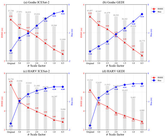
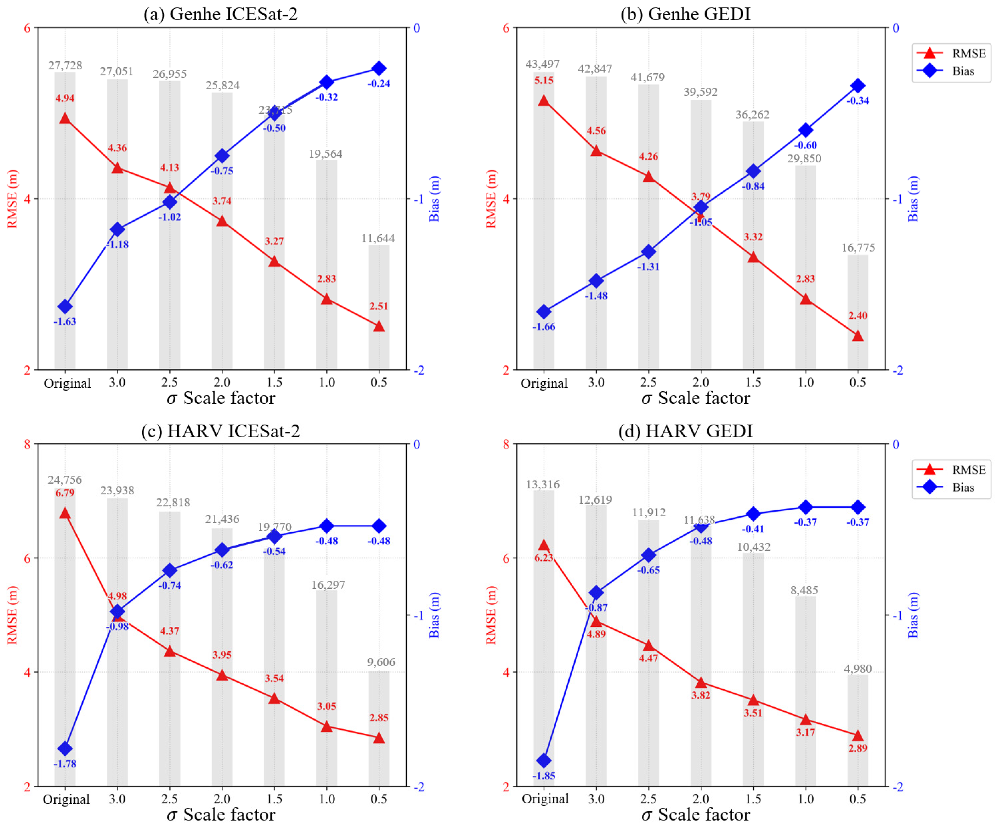
To evaluate the impact of the adaptive truncation threshold on spaceborne LiDAR data refinement, a parameter sensitivity analysis was conducted in the Genhe and HARV study areas. The threshold coefficient $k$ was varied from 0.5 to 3 (denoted as $k\sigma$). Figure 15 illustrates the trade-off curves of the overall RMSE, Bias, and $N$ for both ICESat-2 and GEDI datasets.

Figure 15. Sensitivity analysis of different adaptive truncation thresholds ($\sigma$ scale factors from 0.5 to 3.0). (a) ICESat-2 in Genhe, (b) GEDI in Genhe, (c) ICESat-2 in HARV, (d) GEDI in HARV.

The results indicate that the choice of the truncation threshold directly moderates the trade-off between refined data quality and available data quantity. As the $\sigma$ scale factor decreases, the RMSE for both sensors decreases monotonically in the two study areas. For instance, in the Genhe study area, the RMSE of ICESat-2 observations dropped significantly from 4.94 m to 2.51 m at $0.5\sigma$. However, as a cost of this high-precision filtering, the number of retained valid footprints $N$ drops sharply. At the strictest threshold of $0.5\sigma$, the retention rate of the data is less than 42%. Conversely, when $k\ge 1.5$, although a higher percentage of footprint data is preserved, the overall RMSE exceeds 3.2 m in most cases.

Thus, $k=1$ represents the optimal balance. This threshold not only stably controls the overall RMSE of GEDI and ICESat-2 to approximately 2.8–3.2 m, but also preserves over 63% of the footprints. Therefore, selecting $1\sigma$ as the standard adaptive truncation threshold achieves the most robust and optimal balance between high accuracy and high spatial density.

5.3. Advantages and Limitations of the Refinement Strategy

The spaceborne LiDAR RH98 points refinement strategy assisted by continuous CHMs proposed in this study demonstrates clear advantages in practical applications, but it also has certain objective limitations.

The primary advantages of this strategy are twofold. First, the method exhibits favorable generalizability. Its processing workflow does not rely on local, high-cost ALS data for model training or empirical parameter calibration. Instead, it achieves automated refinement simply by utilizing existing, publicly available large-scale continuous CHM products as physical envelopes. This independence allows the strategy to be applied at a lower cost to vast forest regions lacking ground-measured data. Second, this strategy effectively overcomes the limitations of traditional data filtering, achieving a balance between the accuracy and spatial density of reference points. Through adaptive threshold constraints, this method successfully reincorporates daytime and weak/coverage beam observations, which are typically discarded in conventional processing, into the valid data pool. While ensuring overall data accuracy, it increases the spatial density of available reference points by 1.5 to 4.4 times, providing richer control point support for the spatial interpolation and inversion of large-scale forest parameters. In addition, although external CHMs contain inherent errors, particularly in steep terrain and dense forests, the proposed strategy utilizes the CHM solely as a soft constraint with a broad and adaptive threshold. This mechanism effectively ensures that the refined LiDAR observations remain highly reliable even under moderate prior uncertainty.

However, this refinement strategy also has some limitations in its application. It must be emphasized that this method is inherently a gross error removal technique for data post-processing, rather than a direct numerical calibration of the initial spaceborne observations. It can isolate extreme suspended noise points or ground-penetrating noise caused by cloud cover and strong background light interference, but it cannot eliminate the inherent systematic errors of the spaceborne LiDAR sensors themselves from a physical mechanism perspective (such as the waveform broadening effect of large footprints on sloped terrain). Furthermore, the effectiveness of the algorithm highly depends on the local quality of the external a priori CHM products. In complex forest scenarios with extremely steep terrain or exceptionally tall and dense canopies, the signal penetration capability of spaceborne LiDAR itself is severely limited, and the estimates from external auxiliary CHMs in these regions also tend to exhibit substantial uncertainty. When the reliability of the a priori physical envelope decreases, the determination of the adaptive truncation threshold may deviate, leading to a certain degree of degradation in the optimization performance of this refinement method under such extremely complex scenarios.

Furthermore, the proposed filtering strategy holds significant potential for future large-scale forest height and biomass mapping. Future spaceborne LiDAR and radar missions (such as BIOMASS and NISAR) [4,49] heavily rely on a massive volume of highly accurate forest canopy height control points for model calibration and validation. By successfully reclaiming daytime and weak/coverage beam observations from GEDI and ICESat-2, this method can provide high-density, high-quality reference datasets globally at a low cost. This capability directly supports large-scale biomass estimation and forest carbon stock monitoring, particularly in regions lacking airborne LiDAR data.

Additionally, the applicability of the proposed filtering strategy in global tropical rainforest regions (e.g., the Amazon and Congo basins) represents an important future research direction. Due to the lack of high-resolution and high-accuracy validation datasets (such as local ALS) in these low-latitude zones, a concrete quantitative evaluation could not be conducted at present. Tropical rainforests present unique challenges, including extremely tall trees, dense canopy structures, and continual cloud cover, which often degrade the quality of prior continuous CHM products. Nevertheless, the underlying methodology remains globally transferable. When applying this framework to tropical ecosystems, users can first evaluate and select the most reliable regional CHM product as the prior spatial envelope, and then employ the adaptive filtering strategy to clean the spaceborne LiDAR footprints.

6. Conclusions

To address the limitation of sparse forest height reference point distribution caused by the conventional strict filtering of spaceborne LiDAR data, this study proposes a refinement strategy assisted by an a priori continuous CHM, focusing on its practical application for large-scale forest parameters mapping. By introducing a morphologically consistent global CHM as a reliable external constraint, combined with the $1\sigma$ adaptive truncation of relative height differences, this method effectively removes extreme gross errors from the initial all-available observations. Validation against ALS RH98 indicates that this post-processing strategy stably reduces the overall RMSE to approximately 3 m, effectively mitigating systematic biases caused by limited capability of signal penetration and terrain slopes. Furthermore, it successfully recovers the application value of daytime and weak/coverage beam data, resulting in a final valid reference point density 1.5 to 4.4 times that achieved by traditional strict filtering. Although the optimization performance may degrade in extreme scenarios with exceptionally steep terrain or highly tall and dense canopies due to the uncertainties in the a priori CHM products, this study overall confirms the scientific feasibility of relaxing the filtering conditions for spaceborne LiDAR data. Ultimately, this refinement strategy provides a low-cost and highly transferable approach to overcome the limitation of sparse control points in large-scale forest structure mapping.

References

- Lefsky, M.A. A global forest canopy height map from the Moderate Resolution Imaging Spectroradiometer and the Geoscience Laser Altimeter System. Geophys. Res. Lett. 2010, 37, L15401. [Google Scholar] [CrossRef] [Scilit]
- Huang, H.; Liu, C.; Wang, X.; Biging, G.S.; Chen, Y.; Yang, J.; Gong, P. Mapping vegetation heights in China using slope correction ICESat data, SRTM, MODIS-derived and climate data. ISPRS J. Photogramm. Remote Sens. 2017, 129, 189–199. [Google Scholar] [CrossRef] [Scilit]
- Persson, H.; Olsson, H.; Soja, M.; Ulander, L.; Fransson, J. Experiences from Large-Scale Forest Mapping of Sweden Using TanDEM-X Data. Remote Sens. 2017, 9, 1253. [Google Scholar] [CrossRef] [Scilit]
- Silva, C.A.; Duncanson, L.; Hancock, S.; Neuenschwander, A.; Thomas, N.; Hofton, M.; Fatoyinbo, L.; Simard, M.; Marshak, C.Z.; Armston, J.; et al. Fusing simulated GEDI, ICESat-2 and NISAR data for regional aboveground biomass mapping. Remote Sens. Environ. 2021, 253, 112234. [Google Scholar] [CrossRef] [Scilit]
- Markus, T.; Neumann, T.; Martino, A.; Abdalati, W.; Brunt, K.; Csatho, B.; Farrell, S.; Fricker, H.; Gardner, A.; Harding, D.; et al. The Ice, Cloud, and land Elevation Satellite-2 (ICESat-2): Science requirements, concept, and implementation. Remote Sens. Environ. 2017, 190, 260–273. [Google Scholar] [CrossRef] [Scilit]
- Neuenschwander, A.L.; Magruder, L.A. Canopy and Terrain Height Retrievals with ICESat-2: A First Look. Remote Sens. 2019, 11, 1721. [Google Scholar] [CrossRef] [Scilit]
- Neumann, T.A.; Martino, A.J.; Markus, T.; Bae, S.; Bock, M.R.; Brenner, A.C.; Brunt, K.M.; Cavanaugh, J.; Fernandes, S.T.; Hancock, D.W.; et al. The Ice, Cloud, and Land Elevation Satellite—2 mission: A global geolocated photon product derived from the Advanced Topographic Laser Altimeter System. Remote Sens. Environ. 2019, 233, 111325. [Google Scholar] [CrossRef] [Scilit]
- Brown, M.E.; Arias, S.D.; Chesnes, M. Review of ICESat and ICESat-2 literature to enhance applications discovery. Remote Sens. Appl. Soc. Environ. 2023, 29, 100874. [Google Scholar] [CrossRef] [Scilit]
- Silva, C.A.; Neuenschwander, A.; Hamamura, C.; Godinho, S.; Brock, K.M.; Malambo, L.; Narine, L.; Atkins, J.W.; Borak, J.S.; Popescu, S.; et al. Beyond Ice: NASA’s ICESat-2 spaceborne lidar mission for land and vegetation applications. IEEE Geosci. Remote Sens. Mag. 2026, 14, 2–33. [Google Scholar] [CrossRef] [Scilit]
- Dubayah, R.; Blair, J.B.; Goetz, S.; Fatoyinbo, L.; Hansen, M.; Healey, S.; Hofton, M.; Hurtt, G.; Kellner, J.; Luthcke, S.; et al. The Global Ecosystem Dynamics Investigation: High-resolution laser ranging of the Earth’s forests and topography. Sci. Remote Sens. 2020, 1, 100002. [Google Scholar] [CrossRef] [Scilit]
- Hofton, M.; Blair, J.B. Algorithm Theoretical Basis Document (ATBD) for GEDI Transmit and Receive Waveform Processing for L1 and L2 Products; NASA Goddard Space Flight Center: Greenbelt, MD, USA, 2019. [Google Scholar]
- Neuenschwander, A.; Guenther, E.; White, J.C.; Duncanson, L.; Montesano, P. Validation of ICESat-2 terrain and canopy heights in boreal forests. Remote Sens. Environ. 2020, 251, 112110. [Google Scholar] [CrossRef] [Scilit]
- Liu, A.; Cheng, X.; Chen, Z. Performance evaluation of GEDI and ICESat-2 laser altimeter data for terrain and canopy height retrievals. Remote Sens. Environ. 2021, 264, 112571. [Google Scholar] [CrossRef] [Scilit]
- Urbazaev, M.; Hess, L.L.; Hancock, S.; Sato, L.Y.; Ometto, J.P.; Thiel, C.; Dubois, C.; Heckel, K.; Urban, M.; Adam, M.; et al. Assessment of terrain elevation estimates from ICESat-2 and GEDI spaceborne LiDAR missions across different land cover and forest types. Sci. Remote Sens. 2022, 6, 100067. [Google Scholar] [CrossRef] [Scilit]
- Lang, N.; Jetz, W.; Schindler, K.; Wegner, J.D. A high-resolution canopy height model of the Earth. Nat. Ecol. Evol. 2023, 7, 1778–1789. [Google Scholar] [CrossRef] [Scilit] [PubMed]
- Pauls, J.; Zimmer, M.; Kelly, U.M.; Schwartz, M.; Saatchi, S.; Ciais, P.; Pokutta, S.; Brandt, M.; Gieseke, F. Estimating Canopy Height at Scale. In Proceedings of the 41st International Conference on Machine Learning, Proceedings of Machine Learning Research, Vienna, Austria, 21–27 July 2024; pp. 39972–39988. [Google Scholar]
- Tolan, J.; Yang, H.-I.; Nosarzewski, B.; Couairon, G.; Vo, H.V.; Brandt, J.; Spore, J.; Majumdar, S.; Haziza, D.; Vamaraju, J.; et al. Very high resolution canopy height maps from RGB imagery using self-supervised vision transformer and convolutional decoder trained on aerial lidar. Remote Sens. Environ. 2024, 300, 113888. [Google Scholar] [CrossRef] [Scilit]
- Qi, W.; Dubayah, R.O. Combining Tandem-X InSAR and simulated GEDI lidar observations for forest structure mapping. Remote Sens. Environ. 2016, 187, 253–266. [Google Scholar] [CrossRef] [Scilit]
- Qi, W.; Lee, S.-K.; Hancock, S.; Luthcke, S.; Tang, H.; Armston, J.; Dubayah, R. Improved forest height estimation by fusion of simulated GEDI Lidar data and TanDEM-X InSAR data. Remote Sens. Environ. 2019, 221, 621–634. [Google Scholar] [CrossRef] [Scilit]
- Chen, H.; Cloude, S.R.; White, J.C. Using GEDI Waveforms for Improved TanDEM-X Forest Height Mapping: A Combined SINC + Legendre Approach. Remote Sens. 2021, 13, 2882. [Google Scholar] [CrossRef] [Scilit]
- Choi, C.; Cazcarra-Bes, V.; Guliaev, R.; Pardini, M.; Papathanassiou, K.P.; Qi, W.; Armston, J.; Dubayah, R.O. Large-Scale Forest Height Mapping by Combining TanDEM-X and GEDI Data. IEEE J. Sel. Top. Appl. Earth Obs. Remote Sens. 2023, 16, 2374–2385. [Google Scholar] [CrossRef] [Scilit]
- Qi, W.; Armston, J.; Choi, C.; Stovall, A.; Saarela, S.; Pardini, M.; Fatoyinbo, L.; Papathanasiou, K.; Dubayah, R. Mapping large-scale pantropical forest canopy height by integrating GEDI lidar and TanDEM-X InSAR data. Remote Sens. Environ. 2025, 318, 114534. [Google Scholar] [CrossRef] [Scilit]
- Lei, Y.; Li, W.; Yu, Y.; Liu, X.; Xu, J.; Fu, A.; Wan, J.; Wang, C.; Huang, W.; Qiu, Z.; et al. First demonstration of spaceborne L-band bistatic single-polarization single-baseline SAR interferometry on the retrieval of forest vertical structural information. Remote Sens. Environ. 2025, 329, 114916. [Google Scholar] [CrossRef] [Scilit]
- Tang, H.; Stoker, J.; Luthcke, S.; Armston, J.; Lee, K.; Blair, B.; Hofton, M. Evaluating and mitigating the impact of systematic geolocation error on canopy height measurement performance of GEDI. Remote Sens. Environ. 2023, 291, 13. [Google Scholar] [CrossRef] [Scilit]
- Potapov, P.; Li, X.; Hernandez-Serna, A.; Tyukavina, A.; Hansen, M.C.; Kommareddy, A.; Pickens, A.; Turubanova, S.; Tang, H.; Silva, C.E.; et al. Mapping global forest canopy height through integration of GEDI and Landsat data. Remote Sens. Environ. 2021, 253, 112165. [Google Scholar] [CrossRef] [Scilit]
- Tian, X.; Shan, J. Comprehensive Evaluation of the ICESat-2 ATL08 Terrain Product. IEEE Trans. Geosci. Remote Sens. 2021, 59, 8195–8209. [Google Scholar] [CrossRef] [Scilit]
- Wang, C.; Elmore, A.J.; Numata, I.; Cochrane, M.A.; Shaogang, L.; Huang, J.; Zhao, Y.; Li, Y. Factors affecting relative height and ground elevation estimations of GEDI among forest types across the conterminous USA. GIScience Remote Sens. 2022, 59, 975–999. [Google Scholar] [CrossRef] [Scilit]
- He, L.; Pang, Y.; Zhang, Z.; Liang, X.; Chen, B. ICESat-2 data classification and estimation of terrain height and canopy height. Int. J. Appl. Earth Obs. Geoinf. 2023, 118, 103233. [Google Scholar] [CrossRef] [Scilit]
- Moudr, V.; Gdulová, K.; Gábor, L.; árovcová, E.; Barták, V.; Leroy, F.; Spatenková, O.; Rocchini, D.; Proek, J. Effects of environmental conditions on ICESat-2 terrain and canopy heights retrievals in Central European mountains. Remote Sens. Environ. 2022, 279, 113112. [Google Scholar] [CrossRef] [Scilit]
- Chen, B.; Pang, Y.; Li, Z.; Lu, H.; Liu, L.; North, P.R.J.; Rosette, J.A.B. Ground and Top of Canopy Extraction From Photon-Counting LiDAR Data Using Local Outlier Factor with Ellipse Searching Area. IEEE Geosci. Remote Sens. Lett. 2019, 16, 1447–1451. [Google Scholar] [CrossRef] [Scilit]
- Wang, Y.; Ni, W.; Sun, G.; Chi, H.; Zhang, Z.; Guo, Z. Slope-adaptive waveform metrics of large footprint lidar for estimation of forest aboveground biomass. Remote Sens. Environ. 2019, 224, 386–400. [Google Scholar] [CrossRef] [Scilit]
- Ni, W.; Zhang, Z.; Sun, G. Assessment of Slope-Adaptive Metrics of GEDI Waveforms for Estimations of Forest Aboveground Biomass over Mountainous Areas. J. Remote Sens. 2021, 2021, 9805364. [Google Scholar] [CrossRef] [Scilit]
- Zhang, D.; Chen, Y.; Le, Y.; Dong, Y.; Dai, G.; Wang, L. Refraction and coordinate correction with the JONSWAP model for ICESat-2 bathymetry. ISPRS J. Photogramm. Remote Sens. 2022, 186, 285–300. [Google Scholar] [CrossRef] [Scilit]
- Tian, X.; Shan, J. Detection of Signal and Ground Photons From ICESat-2 ATL03 Data. IEEE Trans. Geosci. Remote Sens. 2023, 61, 5700314. [Google Scholar] [CrossRef] [Scilit]
- Zhao, R.; Ni, W.; Zhang, Z.; Dai, H.; Yang, C.; Li, Z.; Liang, Y.; Liu, Q.; Pang, Y.; Li, Z.; et al. Optimizing ground photons for canopy height extraction from ICESat-2 data in mountainous dense forests. Remote Sens. Environ. 2023, 299, 113851. [Google Scholar] [CrossRef] [Scilit]
- Wang, J.; Shen, X.; Cao, L. Upscaling Forest Canopy Height Estimation Using Waveform-Calibrated GEDI Spaceborne LiDAR and Sentinel-2 Data. Remote Sens. 2024, 16, 2138. [Google Scholar] [CrossRef] [Scilit]
- Jiang, F.; Zhao, F.; Ma, K.; Li, D.; Sun, H. Mapping the Forest Canopy Height in Northern China by Synergizing ICESat-2 with Sentinel-2 Using a Stacking Algorithm. Remote Sens. 2021, 13, 1535. [Google Scholar] [CrossRef] [Scilit]
- Varvia, P.; Korhonen, L.; Bruguière, A.; Toivonen, J.; Packalen, P.; Maltamo, M.; Saarela, S.; Popescu, S.C. How to consider the effects of time of day, beam strength, and snow cover in ICESat-2 based estimation of boreal forest biomass? Remote Sens. Environ. 2022, 280, 113174. [Google Scholar] [CrossRef] [Scilit]
- Zhu, X.; Nie, S.; Wang, C.; Xi, X.; Lao, J.; Li, D. Consistency analysis of forest height retrievals between GEDI and ICESat-2. Remote Sens. Environ. 2022, 281, 113244. [Google Scholar] [CrossRef] [Scilit]
- Li, B.; Xie, H.; Tong, X.; Liu, S.; Xu, Q.; Sun, Y. Extracting accurate terrain in vegetated areas from ICESat-2 data. Int. J. Appl. Earth Obs. Geoinf. 2023, 117, 103200. [Google Scholar] [CrossRef] [Scilit]
- Yang, C.; Peng, D.; Zhang, N.; Chen, M.; Zeng, W.; Sun, X.; Li, L.; Li, W. Performance evaluation and improvement of ICESat-2 and GEDI forest canopy height retrievals in Northeast China. GIScience Remote Sens. 2025, 62, 2497603. [Google Scholar] [CrossRef] [Scilit]
- Chen, R.; Wang, X.; Liu, X.; Wang, S. Optimizing GEDI Canopy Height Estimation and Analyzing Error Impact Factors Under Highly Complex Terrain and High-Density Vegetation Conditions. Forests 2024, 15, 2024. [Google Scholar] [CrossRef] [Scilit]
- Cho, M.-S.; Roy, D.P.; Kashongwe, H.B.; Yan, L.; Shen, M. Assessment and improvement of GEDI canopy height estimation in tropical and temperate forests. Sci. Remote Sens. 2025, 11, 100221. [Google Scholar] [CrossRef] [Scilit]
- Li, W.; Niu, Z.; Shang, R.; Qin, Y.; Wang, L.; Chen, H. High-resolution mapping of forest canopy height using machine learning by coupling ICESat-2 LiDAR with Sentinel-1, Sentinel-2 and Landsat-8 data. Int. J. Appl. Earth Obs. Geoinf. 2020, 92, 102163. [Google Scholar] [CrossRef] [Scilit]
- Liu, X.; Su, Y.; Hu, T.; Yang, Q.; Liu, B.; Deng, Y.; Tang, H.; Tang, Z.; Fang, J.; Guo, Q. Neural network guided interpolation for mapping canopy height of China’s forests by integrating GEDI and ICESat-2 data. Remote Sens. Environ. 2022, 269, 112844. [Google Scholar] [CrossRef] [Scilit]
- Liu, A.; Chen, Y.; Cheng, X. Evaluating ICESat-2 and GEDI with Integrated Landsat-8 and PALSAR-2 for Mapping Tropical Forest Canopy Height. Remote Sens. 2024, 16, 3798. [Google Scholar] [CrossRef] [Scilit]
- Neuenschwander, A.; Pitts, K.; Jelley, B.; Robbins, J.; Markel, J.; Popescu, S.; Nelson, R.; Harding, D.; Pederson, D.; Klotz, B.; et al. Ice, Cloud, and Land Elevation Satellite (ICESat-2) Project Algorithm Theoretical Basis Document (ATBD) for Land-Vegetation Along-Track Products (ATL08); ICESat-2 Project: Lompoc, CA, USA, 2022. [Google Scholar]
- National Ecological Observatory Network. Ecosystem Structure (DP3.30015.001); National Ecological Observatory, N: Gainesville, FL, USA, 2022.
- Quegan, S.; Le Toan, T.; Chave, J.; Dall, J.; Exbrayat, J.-F.; Minh, D.H.T.; Lomas, M.; D’Alessandro, M.M.; Paillou, P.; Papathanassiou, K.; et al. The European Space Agency BIOMASS mission: Measuring forest above-ground biomass from space. Remote Sens. Environ. 2019, 227, 44–60. [Google Scholar] [CrossRef] [Scilit]
Disclaimer/Publisher’s Note: The statements, opinions and data contained in all publications are solely those of the individual author(s) and contributor(s) and not of MDPI and/or the editor(s). MDPI and/or the editor(s) disclaim responsibility for any injury to people or property resulting from any ideas, methods, instructions or products referred to in the content. |
© 2026 by the authors. Licensee MDPI, Basel, Switzerland. This article is an open access article distributed under the terms and conditions of the Creative Commons Attribution (CC BY) license.