Improved Regional Atmospheric Weighted Mean Temperature Modeling Using a Decadal Dataset and Machine Learning Methods over China

Highlights

What are the main findings?

• Developing regional Tm empirical models using two machine learning methods and one-decade hourly ERA5 and various surface observations from meteorological sites substantially improves the accuracy of atmospheric weighted mean temperature estimates.
• The random forest model reduces Tm RMSE by 32% against ERA5 and 25% against radiosonde data, while the Temporal Mixture of Experts with Sequential Attention model achieves reductions of 40% and 33%, respectively, compared with the traditional linear model.

What are the implications of the main findings?

• Comprehensively addressing the limitation incurred by the availability of surface meteorological measurements, the accuracy and coverage of Tm datasets used during modeling, and the diurnal, seasonal, and geographical variations of Tm.
• The proposed machine learning models can provide high-accuracy Tm estimates for reliable GNSS-PWV retrieval.

Abstract

Accurate estimation of the weighted mean temperature (Tm) is essential for retrieving precipitable water vapor (PWV) from ground-based Global Navigation Satellite System (GNSS) observations. Machine learning (ML) techniques excel in modeling nonlinear relationships among Tm time series, station geographic coordinates, and surface meteorological parameters, and recent studies have demonstrated that ML and neural network models outperform conventional linear Tm models. However, the full potential of surface meteorological measurements at GNSS stations for high-precision Tm retrieval remains to be fully explored. This study develops regional Tm empirical models using two ML methods—random forest (RF) and Temporal Mixture of Experts with Sequential Attention (TMESA)—to generate reliable real-time Tm estimates and enhance the accuracy of operational GNSS-PWV retrievals over China. A traditional linear model is adopted as the baseline to evaluate the performance improvements of the proposed models. The models are trained and tested using 10-year (2014–2023) hourly ERA5-derived Tm products and in-situ surface pressure, temperature, and relative humidity from 2377 meteorological stations, with Tm diurnal variations, station coordinates, and day of year integrated as auxiliary predictive features. Validation is conducted using 2024 ERA5 reanalysis data and radiosonde profiles from 120 stations across China. Results show that the RF model yields a bias (RMSE) of −0.11 K (2.67 K) against ERA5 and −0.21 K (2.67 K) against radiosonde data, while the TMESA model achieves superior performance with bias (RMSE) of −0.02 K (2.34 K) and 0.09 K (2.46 K), respectively, whose performance levels comparable to state-of-the-art studies. Compared with the traditional linear model, the RF model reduces Tm RMSE by 32% against ERA5 and 25% against radiosonde data, while the TMESA model achieves reductions of 40% and 33%, respectively. These findings confirm that the proposed ML models can provide high-accuracy Tm estimates for reliable GNSS-PWV retrieval. Future work will focus on the operational application of these models for near-real-time GNSS-PWV estimation.

1. Introduction

As an indicator of the total atmospheric water vapor content, precipitable water vapor (PWV) plays a crucial role in weather forecasting and climate prediction [1,2,3,4]. With global warming and the increasing frequency of extreme weather events, precise monitoring of PWV has become particularly important [5]. The Global Navigation Satellite System (GNSS) offers unique advantages such as all-weather operation, high consistency, and low cost, which meet the requirements of high-precision PWV monitoring. PWV derived from GNSS can achieve a temporal resolution of up to minutes with an accuracy of 1–2 mm [6]. The weighted average temperature (Tm) of the atmosphere is a key variable for retrieving PWV by ground-based GNSS [7]. A critical issue with Tm bias is its spurious large diurnal cycle, which arises from the diurnally invariant relationship between Tm and surface air temperature (Ts) coupled with significant diurnal variations in Ts. This bias can induce an artificial diurnal cycle in PWV and cause 1–2% day/night discrepancies in PWV estimates [8]. Therefore, the accuracy of Tm estimation is of paramount significance for improving the precision of PWV retrieval.

Various methods have been employed to construct Tm models. Bevis et al. [7] established a linear regression formula (hereafter referred to as the Bevis-Tm model) between Tm and Ts by analyzing 8718 sounding records over a 2-year period from 13 radiosonde stations in North America. With the advancement of research, nonlinear relationships between Tm and Ts have been explored, along with their correlations with geographical location, season, and other meteorological factors. Neural networks and machine learning techniques possess powerful nonlinear fitting capabilities, enabling them to automatically learn complex nonlinear relationships within datasets. For instance, Ding [9] developed a global Tm model using a multilayer feedforward neural network and integrating two key characteristics of Tm, which are its seasonal variations and its relationships with surface meteorological variables. This model demonstrated higher accuracy than the GTrop-Tm model [10] and the neural network (NN) model [11]. Cai et al. [12] built hybrid Tm models with BPNN, RF and GRNN using radiosonde profiles at 150 stations from 2007 to 2016, and the RF model attained an RMSE of 2.70 K. Since the hybrid method relies on UNB3m as baseline input, systematic errors from low-resolution lookup tables are inevitably introduced. Li et al. [13] evaluated RF, LightGBM, SVM and CART for Tm retrieval based on radiosonde data at seven stations in Yangtze River Delta from 2014 to 2019, confirming LightGBM as the best performer (daily RMSE = 1.85 K). Although these works prove the superiority of ensemble learning, they suffer from flawed hybrid frameworks or insufficient study regions. Zhu et al. [14] constructed a Tm model over China using a feedforward neural network algorithm based on the fifth generation European Centre for Medium-Range Weather Forecasts (ECMWF) atmospheric reanalysis of the global climate (ERA5). Compared with two well-recognized Tm models, Ctrop-Tm [15] and GPT3-Tm [16], this model showed significant improvements in Tm retrieval. Zhao et al. [17] established a Tm model over China using the long short-term memory (LSTM) architecture, based on ERA5 data from 2017 to 2020. This model achieved higher accuracy than three common traditional Tm models, UNB3-Tm [18], GPT3-Tm, and the Bevis-Tm model. Huang et al. [19] developed a Tm model over China using random forest, based on datasets predicted by the AI weather model Pangu-Weather. This model outperformed GPT3-Tm, the Bevis-Tm model, and the Tm forecast model developed using a backpropagation neural network in terms of Tm estimation performance. In addition to machine learning-based Tm modeling strategies, spectral analysis methods also provide a viable alternative for characterizing the temporal variations of Tm. Ma et al. [20] proposed the LCTm model by adopting the anti-leakage least-squares spectral analysis (ALLSSA) method, utilizing ERA5 reanalysis datasets from 2015 to 2019. The model achieves an Tm RMSE of 2.06 K when validated against ERA5, whereas its error degrades to 3.47 K when evaluated with independent radiosonde observations. Nevertheless, these machine learning studies [14,17,19] primarily relied on single-source reanalysis or AI model predictions without exploiting multi-source, decade-long observations from dense nationwide meteorological networks.

Based on the datasets used for Tm modeling, Tm models can generally be categorized into two types, namely those established primarily using radiosonde observations [7,9,11,21,22,23] and those developed using reanalysis datasets [12,17,24,25,26,27,28]. These existing models are limited by the availability of surface air temperature measurements, the accuracy and coverage of Tm datasets used during modeling, and the diurnal variations in Tm [8,19]. Recent studies have further highlighted the importance of elevation correction and regional adjustment strategies. Zhang et al. [29] proposed the RGTm model combining ERA5, radiosonde data, and TanDEM-X 90 m DEM products over China, addressing ERA5’s lowest-level height deviations and achieving 12.2% accuracy improvement over GPT3. Zhang et al. [30] developed the EurTm model for Europe through least squares optimization of HGPT2 with surface temperature residuals and diurnal variation terms, yielding 32.7% RMSE improvement. However, this approach requires real-time global model outputs and local radiosonde access, limiting applicability for operational networks with only surface meteorological sensors.

The aforementioned studies reveal persistent gaps: (1) RF-based models have not been scaled to nationwide, decade-long operational frameworks free from empirical baseline dependencies; (2) spectral methods capture periodic signals but struggle with nonlinear interactions and cross-source generalization; (3) regional adjustment strategies improve accuracy but depend on external model outputs unavailable in real time; and (4) the potential of directly integrating ERA5 with dense nationwide surface meteorological networks via machine learning remains untapped.

To enhance the nationwide PWV measurement capability, the China Meteorological Administration has deployed over 1600 ground-based GNSS stations collocated with meteorological instruments to measure surface air pressure, temperature, and relative humidity. By the end of 2026, the number of ground-based GNSS stations for PWV observation in China will exceed 2300, with an additional 700 stations to be added. In recent years, more reliable Tm estimates can be derived from modern reanalysis data, such as ERA5. Furthermore, high-quality measurements of surface meteorological variables (e.g., temperature, humidity, and rainfall) have been available for several decades at more than 2300 national surface meteorological stations across China. Together, the availability of decade-long ERA5 reanalysis, nationwide surface meteorological networks, and mature ensemble learning methods offers a pathway to fill the aforementioned gaps. It is therefore essential to improve atmospheric weighted mean temperature modeling over China using these new datasets, thereby enhancing the accuracy of near real-time PWV retrievals from the national GNSS PWV observation network.

The purpose of this paper is to develop a regional Tm empirical model that provides more reliable real-time Tm estimates, thereby improving the accuracy of operational PWV estimates over China. A traditional linear regression model and two machine learning methods are employed to construct regional Tm models for China. The input datasets for Tm modeling include hourly Tm retrievals from ERA5 and hourly surface meteorological variables including pressure, temperature, relative humidity, precipitation, and maximum wind speed over a decade from 2014 to 2024. Tm diurnal variations, station geographical coordinates, and day of the year are considered during model construction. Additionally, sounding profiles from 120 radiosonde stations and ERA5 across China in 2024 are used to validate the accuracy of the Tm models.

The rest of this paper is organized as follows: Section 2 describes the input datasets and methods for Tm modeling. Section 3 details the Tm modeling process, as well as the comprehensive evaluation and analysis of model performance. Section 4 presents results. Section 5 is discussion to interpret the results. Finally, conclusions are summarized in Section 6.

2. Data and Methods

In this study, the ERA5-derived Tm estimates and surface meteorological observations across China from 2014 to 2023 were used for developing and testing Tm models. The surface observations include hourly surface air temperature, relative humidity, pressure, hourly precipitation, and hourly maximum wind speed. The developed Tm models were validated using datasets over China in 2024, which include surface meteorological observations, as well as Tm datasets retrieved from ERA5 and radiosonde meteorological profiles.

2.1. Reanalysis Data

Tm estimates retrieved from ERA5 were used as one of the inputs for Tm modeling. ERA5 is a high-resolution global atmospheric reanalysis product that combines model data with global observations into a complete and consistent global dataset based on the laws of physics [31]. It covers the period from 1940 to the present, with a spatial resolution of 0.25° × 0.25°, vertical coverage ranging from 1000 hPa to 1 hPa (encompassing 37 pressure levels in total), and an hourly temporal resolution. The data are typically released with a latency of approximately five days. Owing to its high spatiotemporal resolution and superior data quality, ERA5 has become a crucial foundational dataset for atmospheric science research, particularly in studies related to ground-based GNSS PWV retrieval [32]. In this study, hourly ERA5 variables, including temperature, relative humidity, and geopotential height across 37 pressure levels, were used to calculate Tm values over China from 2014 to 2024. Sun et al. [33] indicated that Tm derived from ERA5 exhibits higher accuracy than that derived from other reanalysis datasets (e.g., MERRA-2, JRA-55, and CRA40), and it is recommended as the preferred dataset for climate research in China.

2.2. Surface Meteorological Observations and Radiosonde Meteorological Profiles

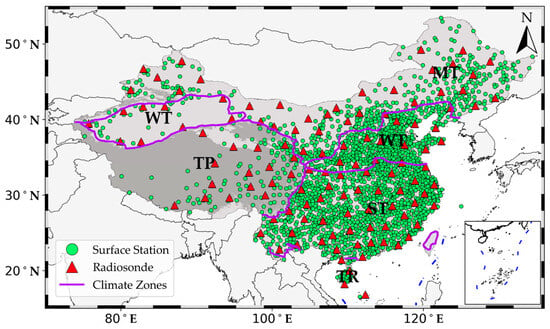
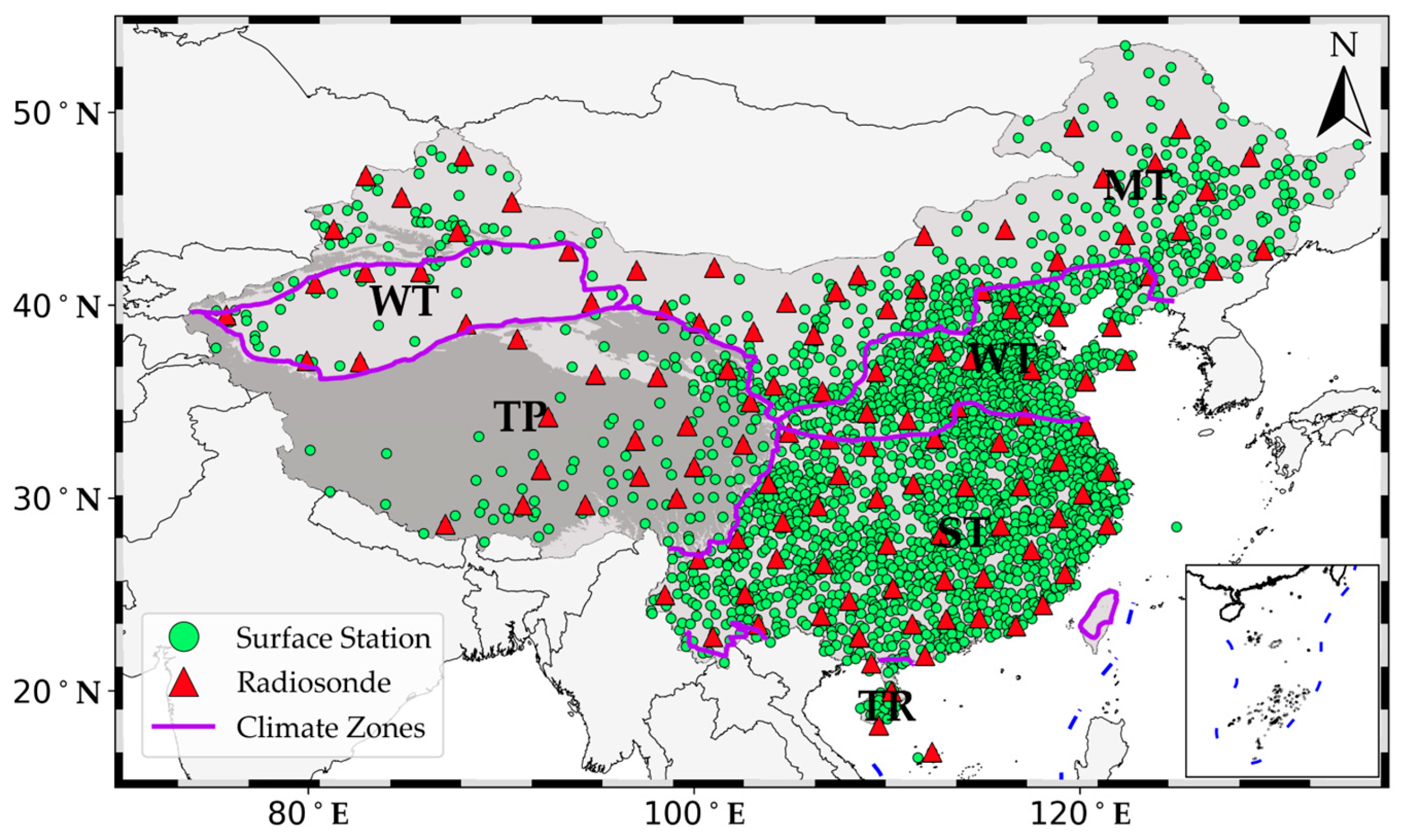
Hourly surface meteorological observations including surface air temperature, relative humidity, pressure, precipitation, and maximum wind speed in 2377 stations over China from 2014 to 2024 were obtained from the National Meteorological Science Data Center (NMSDC, https://data.cma.cn/). Among these stations, 1467 sites are located at altitudes below 500 m, 623 sites at altitudes between 500 m and 1500 m, 229 sites at altitudes between 1500 m and 3500 m, and 58 sites at altitudes above 3500 m. This distribution ensures that the surface meteorological stations used in this study have representative coverage across China. The geographical distribution of these surface meteorological stations is displayed in Figure 1. Rigorous operational quality control procedures were applied to these meteorological observations, and only high-quality data were used in the study. The ranges of the hourly surface meteorological variables are as follows, surface air temperature from −50.6 to 48.5 °C, relative humidity from 1% to 100%, pressure from 542.4 to 1063.9 hPa, hourly precipitation from 0 to 201.9 mm, and hourly maximum wind speed from 0 to 42.1 m/s. Detailed statistical information on these surface meteorological variables is provided in Table 1.

Figure 1. Geographical distribution of 2377 surface meteorological stations (green solid circles) and 120 radiosonde stations (red triangles) over China. Purple solid lines denote the boundaries of climate zones, namely tropical zone (TR), subtropical zone (ST), warm temperate zone (WT), mid-temperate zone (MT), and Tibetan Plateau (TP).

Table 1. Characteristics of hourly surface meteorological variables over China from 2014 to 2024, including surface air temperature (Ts), relative humidity (RHU), pressure (PRS), hourly precipitation (PRE), and hourly maximum wind speed (WIN_S_Max).

	Ts (°C)	RHU (%)	PRS (hPa)	PRE (mm)	WIN_S_Max (m/s)
Min	−50.6	1	542.4	0	0
Max	48.5	100	1063.9	201.9	42.1

Radiosonde meteorological profiles from 120 stations across China in 2024 were also obtained from NMSDC. Quality control procedures were performed on these profiles, and all profiles have a high temporal resolution (note: radiosonde observations are typically recorded at minute intervals during balloon ascent, corresponding to a de facto minutely temporal resolution). Generally, radiosonde stations operated by the China Meteorological Administration (CMA) release meteorological balloons twice a day, at 00:00 UTC and 12:00 UTC, respectively. Some stations additionally release one or two more meteorological balloons at 06:00 UTC and/or 18:00 UTC. Radiosonde observations, including relative humidity, pressure, and temperature, were used to calculate Tm values, which were treated as true values for validating the Tm models in this study. The geographical distribution of the radiosonde stations is also shown in Figure 1. Overall, the surface meteorological stations and radiosonde stations are evenly distributed across China, except for regions such as the western Tibetan Plateau and the desert areas of western China, where stations are sparse.

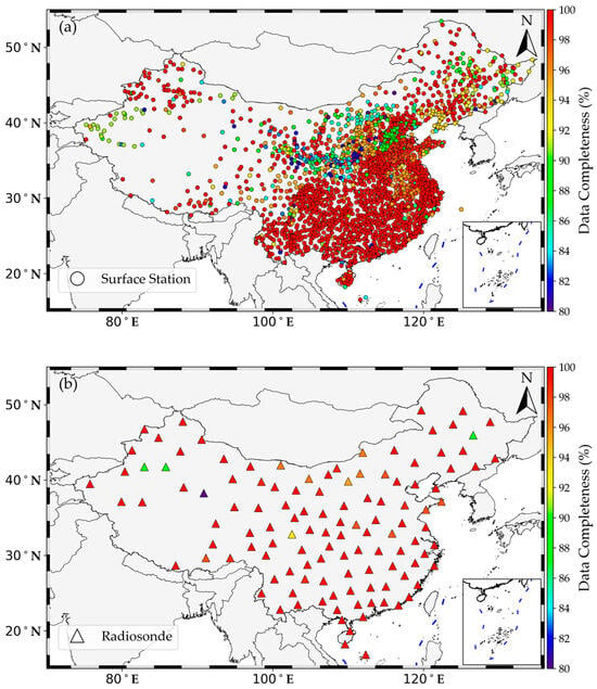
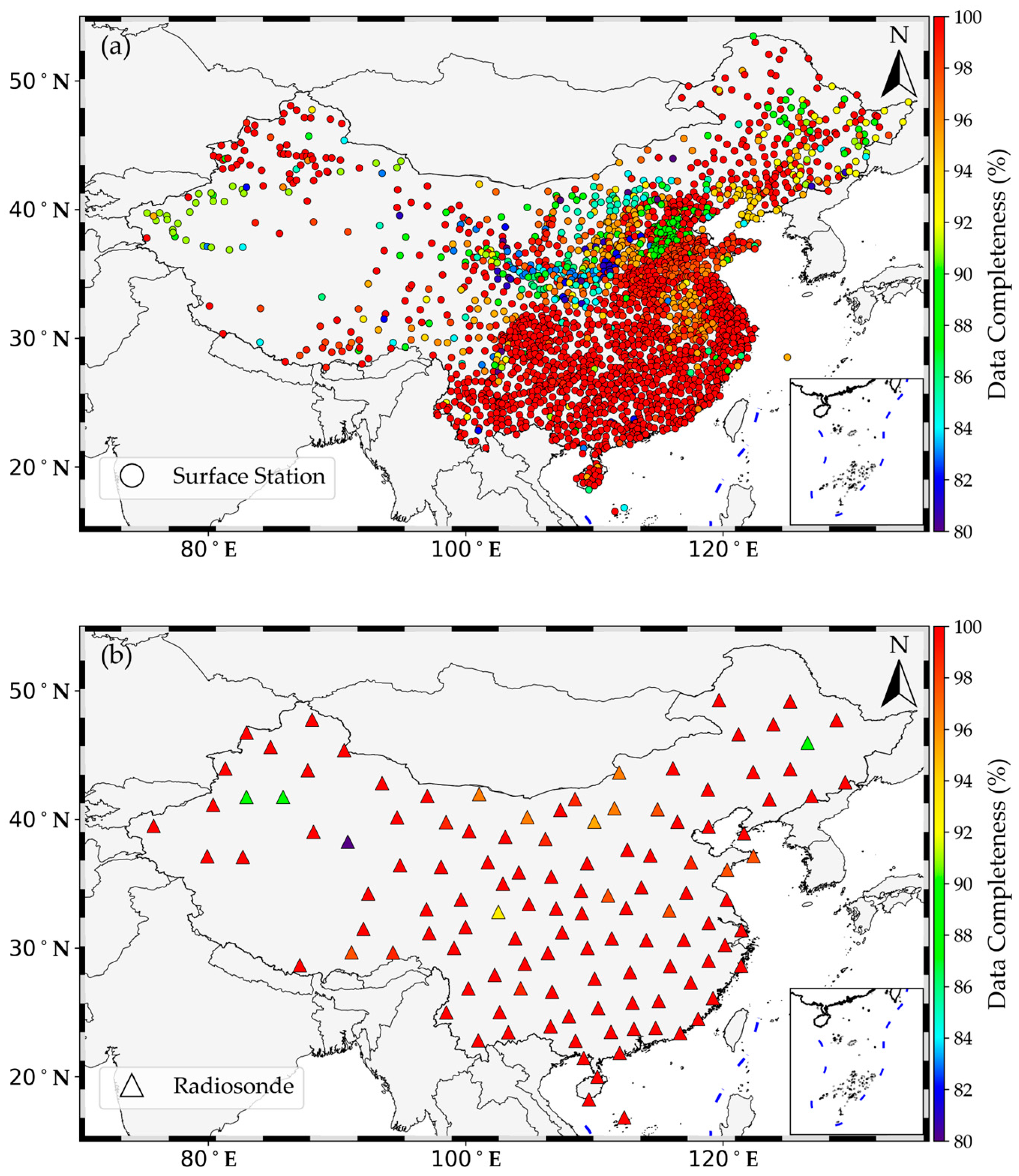
Data completeness for each surface meteorological station from 2014 to 2024 and for each radiosonde station in 2024 over China are illustrated in Figure 2. Most surface stations exhibit data completeness above 90%, except for some stations in central and western China, where completeness is slightly lower but still above 80%. Data completeness also exceeds 90% for most radiosonde stations.

Figure 2. Data completeness of (a) surface meteorological stations from 2014 to 2024 and (b) radiosonde stations in 2024 over China.

2.3. Tm Retrievals from ERA5 and Radiosonde

PWV (in mm) at one ground-based GNSS station can be estimated by a linear function of zenith wet delay (ZWD) [7]:

$$PWV=ZWD·\mathsf{\Pi }=ZWD·{10}^6/\left[{\rho }_w{R}_v\left({\displaystyle \frac{k_3}{T_m}}+k_2^{\prime }\right)\right]$$

(1)

where ${\rho }_w=1000$ kg m⁻³ is the density of liquid water, $R_v=461.525$ J K⁻¹ kg⁻¹ is the specific gas constant for water vapor, $k_3=3.739\times {10}^5$ K2 hPa⁻¹ and $k_2^{\prime }=22$ K hPa⁻¹ are the refraction constants, and $T_m$ is the weighted mean temperature (in K) [7,34], defined as

$$T_m={\displaystyle \frac{\int \left(e/T\right)dz}{\int \left(e/T^2\right)dz}}$$

(2)

where $e$ is the partial pressure of water vapor (in hPa), and $T$ is the atmospheric temperature (in K).

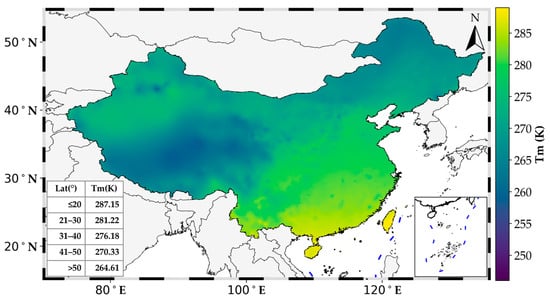
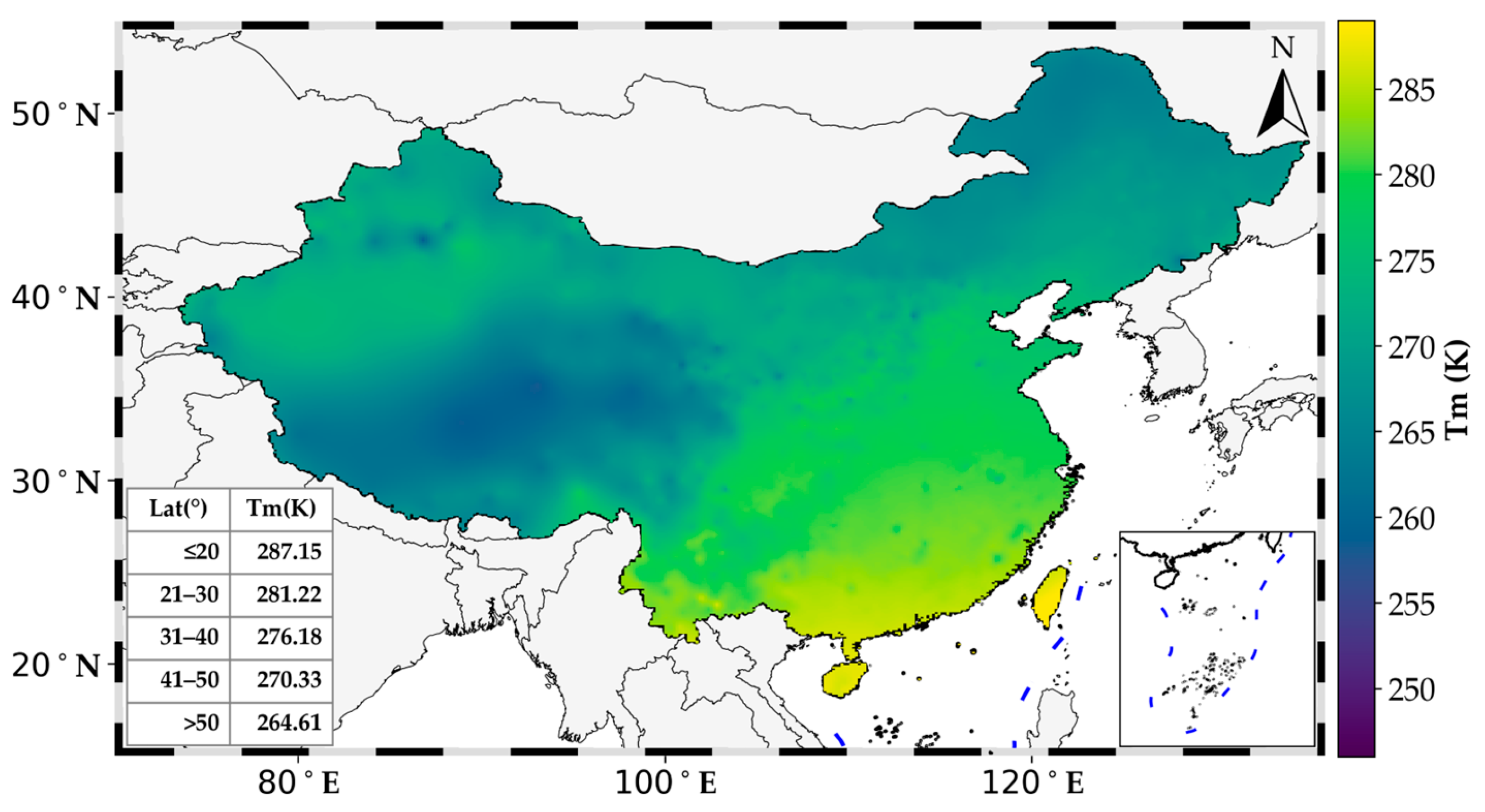
The Tm retrievals at each surface meteorological station are derived from ERA5 reanalysis using the method described by Zhang et al. [32]. The geographical distribution of the mean Tm derived from ERA5 during the period from 2014 to 2024 is shown in Figure 3. The mean Tm values are between 258.0 and 288.3 K over China. The mean Tm values are generally lager than 275 K in southeastern China, and substantially higher than those in northeastern China, where they typically range between 265 K and 275 K. The lowest Tm occurs over the central Tibetan Plateau, falling below 260 K, owing to its average elevation above 3000 m and cold high-altitude climate.

Figure 3. Geographical distribution of average Tm derived from ERA5 during the period from 2014 to 2024. The average values of Tm distributed with latitudes are presented in the inset box.

2.4. Tm Modeling Methods

Three models, namely the linear regression, random forest (RF) and Temporal Mixture of Experts with Sequential Attention (TMESA) models, are employed to estimate Tm. First, the Tm linear regression model, proposed by Bevis et al. [7], assumes a linear relationship between Tm (in K) and surface air temperature Ts (in K). This model is expressed as follows:

$$T_m=a·T_s+b$$

(3)

where $a$ and $b$ are undetermined coefficients.

Second, the RF model is an ensemble machine learning algorithm designed for regression tasks, first proposed by Tin Kam [35]. During RF training, multiple decision trees are constructed using bootstrap aggregation (bagging) to generate a modal prediction for classification or a mean prediction for regression. Thanks to its adaptive decision-making rules, the RF model excels at capturing nonlinear relationships between the dependent variable and multiple independent variables, even in the presence of complex environmental factors. This capability enables the RF model to deliver excellent predictive performance [36]. In this study, we adopt the RF-based Tm estimation framework presented by Huang et al. [19]. However, we utilize different input datasets for model training and validation.

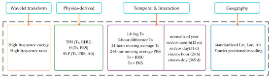
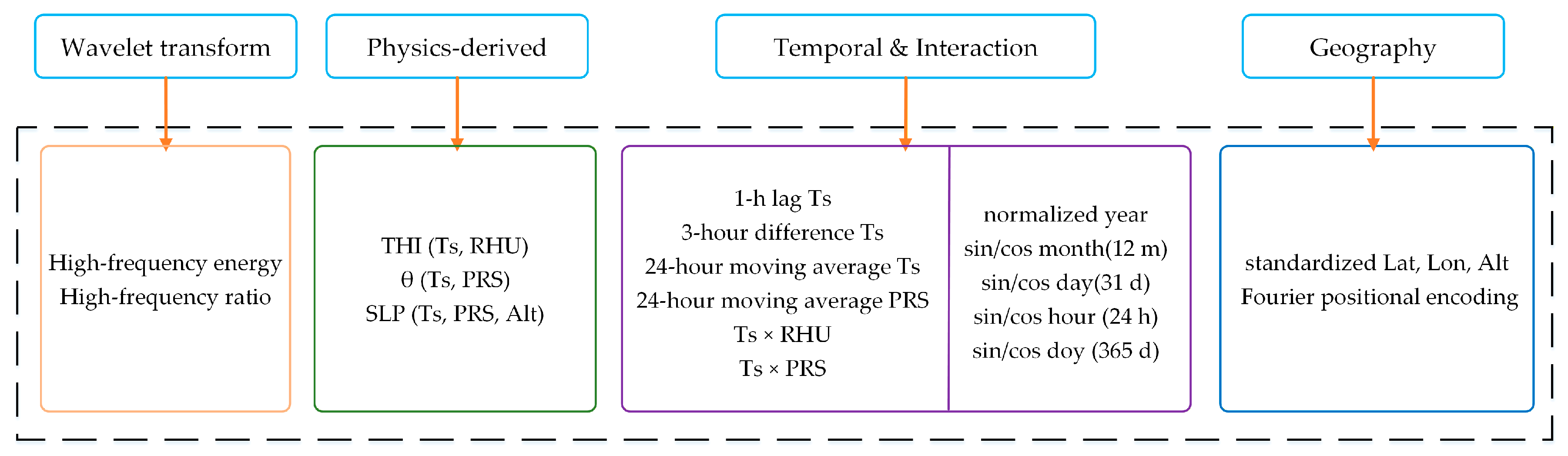
Third, the TMESA model is a deep learning architecture designed for temporal sequence forecasting. It integrates the Sparse Mixture of Experts (Sparse MoE) framework, originally proposed by Jacobs et al. [37] and later enhanced with sparsity mechanisms by Shazeer et al. [38]. During TMESA training, a trainable gating network assigns input samples to the Top-K most relevant expert subnetworks through sparse routing, activating only a subset of the total parameters while maintaining approximately constant computational cost despite expanding model capacity. Benefiting from sparse activation patterns and load-balancing constraints, TMESA effectively captures complex nonlinear relationships between dependent variables and high-dimensional independent variables under complicated spatiotemporal environmental conditions, thus delivering superior prediction accuracy with improved parameter efficiency [39]. In this study, we adopt this architecture with integrated ExpertBlock modules (i.e., Expert-i) and quantile regression outputs, using sequential meteorological datasets to estimate Tm. The TMESA framework is illustrated in Figure 4. A feature enhancement step is applied to the input dataset (Figure 5). The temperature–humidity index (THI), potential temperature (θ), and sea-level pressure (SLP) are introduced to enrich the input features. The formulas for computing these three variables are presented below.

$$THI=Ts-0.55\times \left(1-{\displaystyle \frac{RHU}{100}}\right)\times \left(Ts-14.5\right)$$

(4)

$$\theta =Ts\times {\left({\displaystyle \frac{1000}{PRS}}\right)}^{0.286}$$

(5)

$$SLP={PRS\times \left(1+{\displaystyle \frac{0.0065\times Alt}{Ts\times 0.0065\times Alt}}\right)}^{-5.257}$$

(6)

where Ts, RHU, PRS, and Alt represent surface air temperature, relative humidity and pressure, and altitude at each station, respectively. In addition, we apply wavelet transform to extract high-frequency energy and high-frequency ratio from the input datasets. We also construct several temporal and interaction terms, including the 1 h lag of Ts, 3 h difference of Ts, 24 h moving average of Ts and PRS, surface air temperature multiplied by relative humidity (Ts × RHU), surface air temperature multiplied by pressure (Ts × PRS), and so forth. The Fourier positioning encoding technique is adopted to provide continuous and periodic representations of geographic location information and enhance the model’s ability to capture spatial heterogeneity.

Figure 4. The framework of Temporal Mixture of Experts Sequential Attention (TMESA) model. In this framework, B, T, D and E are batch size, time step, and dimension and the number of experts, respectively. [x,h] indicate the number of the original features and that of the hidden layer features, respectively. MLP represents multilayer perceptron.

Figure 5. Flowchart of data feature enhancement procedure. THI, θ, and SLP indicate temperature–humidity index, potential temperature, and sea level pressure, respectively. Ts, RHU and PRS represent surface air temperature, relative humidity and pressure, respectively. Lat, Lon, and Alt stand for latitude, longitude, and altitude, respectively.

2.5. Tm Model Evaluation Methods

The bias, root-mean-square error (RMSE) and correlation coefficient (r) are used to evaluate Tm model accuracy.

$$\mathrm{B}\mathrm{i}\mathrm{a}\mathrm{s}={\displaystyle {\sum }_{i=1}^n}\left(P_i-O_i\right)/n$$

(7)

$$\mathrm{R}\mathrm{M}\mathrm{S}\mathrm{E}=\sqrt{{\displaystyle {\sum }_{i=1}^n}{{(P}_i-O_i)}^2/n}$$

(8)

$$={\displaystyle \frac{{\sum }_{i=1}^n\left(O_i-\overline{O}\right)\left(P_i-\overline{P}\right)}{\sqrt{{{\sum }_{i=1}^n\left(O_i-\overline{O}\right)}^2}\sqrt{{{\sum }_{i=1}^n\left(P_i-\overline{P}\right)}^2}}}$$

(9)

where P and O are predicted value by Tm model and observed value, respectively. The symbol n and i are the total number of samples and the serial number of the samples, respectively. $\overline{P}$ and $\overline{O}$ are the average value of P and O, respectively.

3. Tm Model Construction

In this study, we apply two machine learning methods, namely RF and TMESA, to train Tm models. The datasets including ERA5-derived Tm estimates and surface meteorological observations over China from 2014 to 2022 are employed to train the machine learning model. The datasets with the same variables in 2023 are used to test the Tm model. Totally, there are 177,139,624 data samples for training the machine learning models, and 20,577,501 data samples for model testing. The development of the RF Tm model consists of three key steps: feature selection, parameter optimization, and model training. Feature selection is first, conducted via correlation analysis with Tm retrieved by ERA5, where Ts, pressure, relative humidity, hourly maximum wind speed, hourly precipitation, year, month, day, day of year, hour and station longitude, latitude and altitude are adopted as input features.

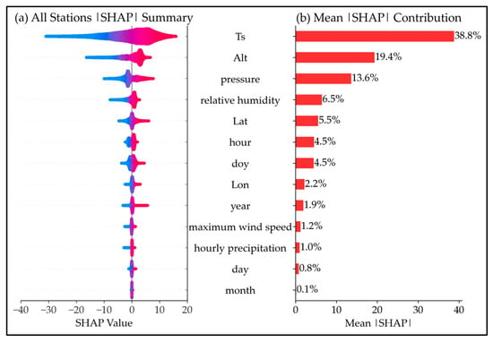
The Shapley additive explanation (SHAP) method [40] is employed for feature importance analysis aiming to optimize feature selection during RF model construction. The input variables including Ts, pressure and site altitude are the ones that provide the most impacts on the predictions according to their associated Shapley values, i.e., 38.8% for Ts, 19.4% for site altitude and 13.6% for pressure (Figure 6). The total contribution of these three variables to Tm prediction is 71.8%. In contrast, year, hourly maximum wind speed, hourly precipitation, day, and month exert only minor influences on the predictions, with mean contributions of 1.9%, 1.2%, 1.0%, 0.8%, and 0.1%, respectively. Accordingly, hourly maximum wind speed and hourly precipitation can be omitted from Tm model training. These variables are often difficult to acquire because many GNSS stations are only equipped with temperature, pressure, and relative humidity sensors. The RF model hyperparameters are optimized using HalvingRandomSearchCV with successive halving strategy, with the search space defined as: n_estimators ∈ {2000, 4000, 6000, 8000, 10,000}, max_depth ∈ {6, 8, 10}, min_samples_leaf ∈ {300, 400, 500, 600}, max_features ∈ {0.6, 1.0}, and min_impurity_decrease ∈ {1 × 10⁻⁴, 5 × 10⁻⁴, 1 × 10⁻³, 2 × 10⁻³}. The optimal parameters are selected based on minimum RMSE on the 2023 validation set. Although year, month, and day have small individual SHAP contributions (1.9%, 0.1%, and 0.8%), they are retained because they encode temporal structures that enable the model to capture nonlinear seasonal and interannual variations in Tm. In contrast, wind speed and precipitation are excluded due to their negligible SHAP values (1.2% and 1.0%) and the fact that existing GNSS stations are typically equipped only with temperature, pressure, and humidity sensors, lacking wind and precipitation measurement capabilities. Ultimately, the variables adopted for Tm modeling include Ts, pressure, relative humidity, year, month, day, day of year, and station longitude, latitude, and altitude. In previous Tm modeling studies, only a small number of parameters were typically employed, such as Ts [7]; Ts and latitude [41]; Ts, surface water vapor pressure, and day of year [28]; and Ts, longitude, latitude, altitude, hour, and day of year [19]. Consequently, the model developed in this study is more comprehensive and versatile.

Figure 6. Feature importance analysis using Shapley additive explanation method (SHAP) for RF model construction. In panel (a), colors indicate feature values from low (blue) to high (red).

4. Results

4.1. Performance of Tm Models

The linear Tm model was fitted using datasets consisting of hourly Tm (in K) retrieved from ERA5 and hourly Ts (in K) observations collected from 2377 surface meteorological stations across China from 2014 to 2023. This yielded a total of 197,717,125 Ts–Tm pairs. The fitted model for China is presented as follows:

$$T_m=0.76T_s+59.51$$

(10)

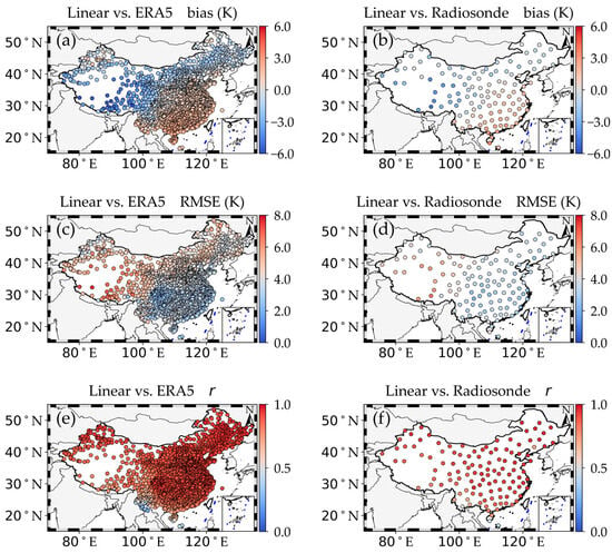
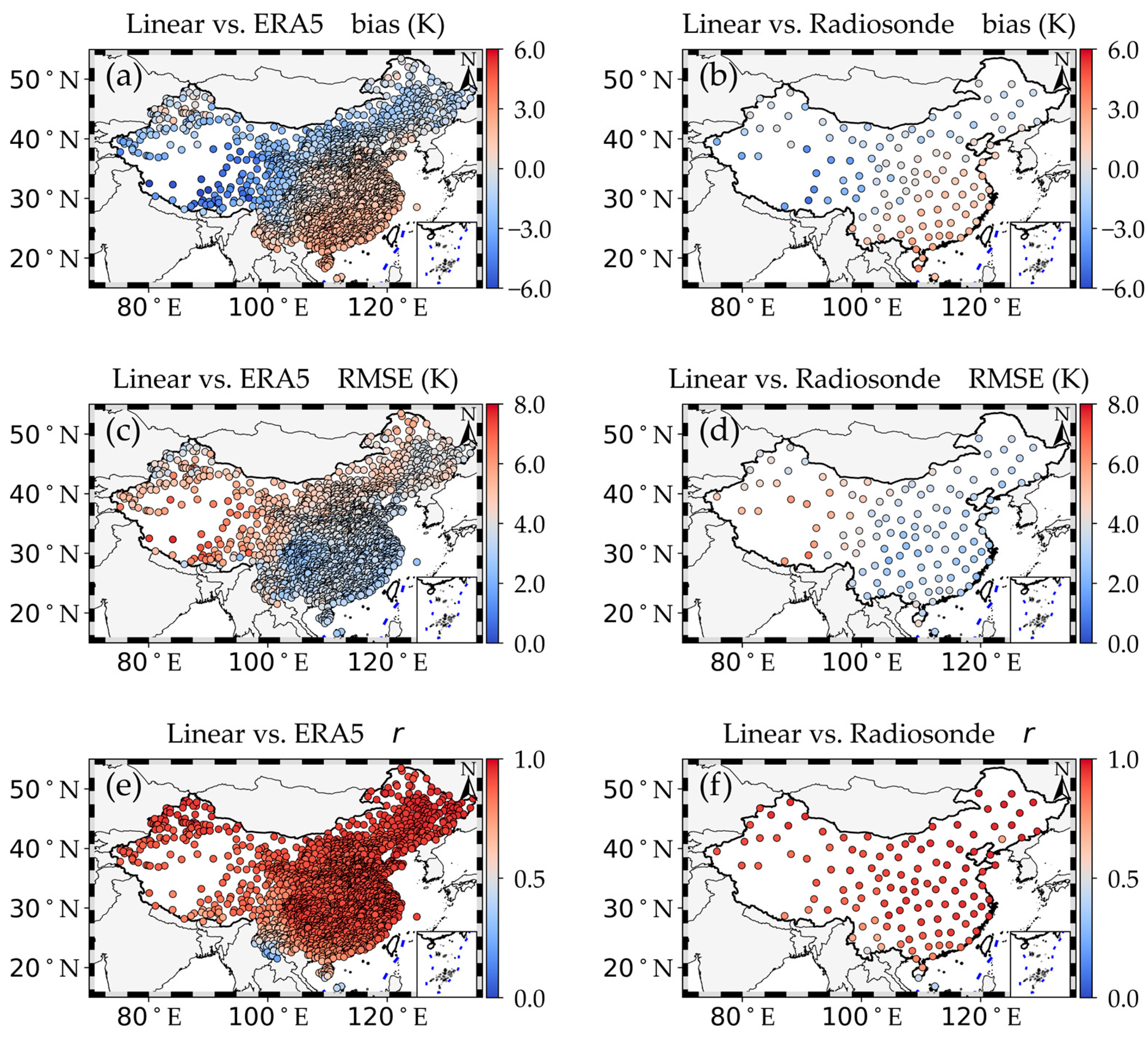
For model validation, datasets including ERA5-Tm, Ts from 2377 stations, and Tm derived from radiosonde meteorological profiles in 2024 were employed. Compared with ERA5 (Figure 7a), the linear model exhibits a warm bias ranging from 0 K to 3 K in southern China. In contrast, a cold bias ranging from 0 K to −4.0 K is observed in most parts of northern China, with the maximum cold bias reaching −6.32 K over the Tibetan Plateau. In central China, the Tm bias is small, ranging between −1.0 K and 1.0 K. Additionally, the Tm RMSE of the linear model validated against ERA5 is shown in Figure 7c. The Tm RMSE in southern China is much smaller than that in northern China, with the maximum Tm RMSE of 7.6 K observed over the Tibetan Plateau. In most parts of China, the correlation coefficients (r) of Tm between the linear model and ERA5 are greater than 0.7, except for regions in southwestern China where the minimum r value is 0.22 (Figure 7e). In addition, the patterns of Tm bias, Tm RMSE, and r for the linear model relative to radiosonde observations are comparable to those relative to ERA5 (Figure 7b,d,f).

Figure 7. Geographical distribution of the Tm bias of the linear model relative to (a) ERA5 and (b) radiosonde observations, Tm RMSE relative to (c) ERA5 and (d) radiosonde observations, and correlation coefficients between the linear model and (e) ERA5 as well as between the linear model and (f) radiosonde observations over China in 2024.

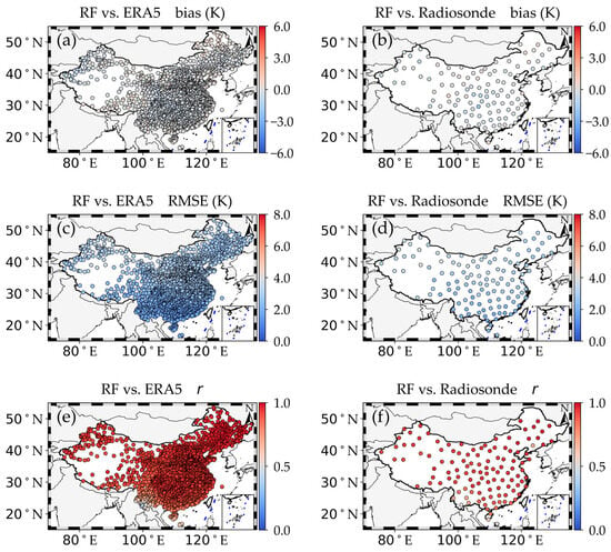
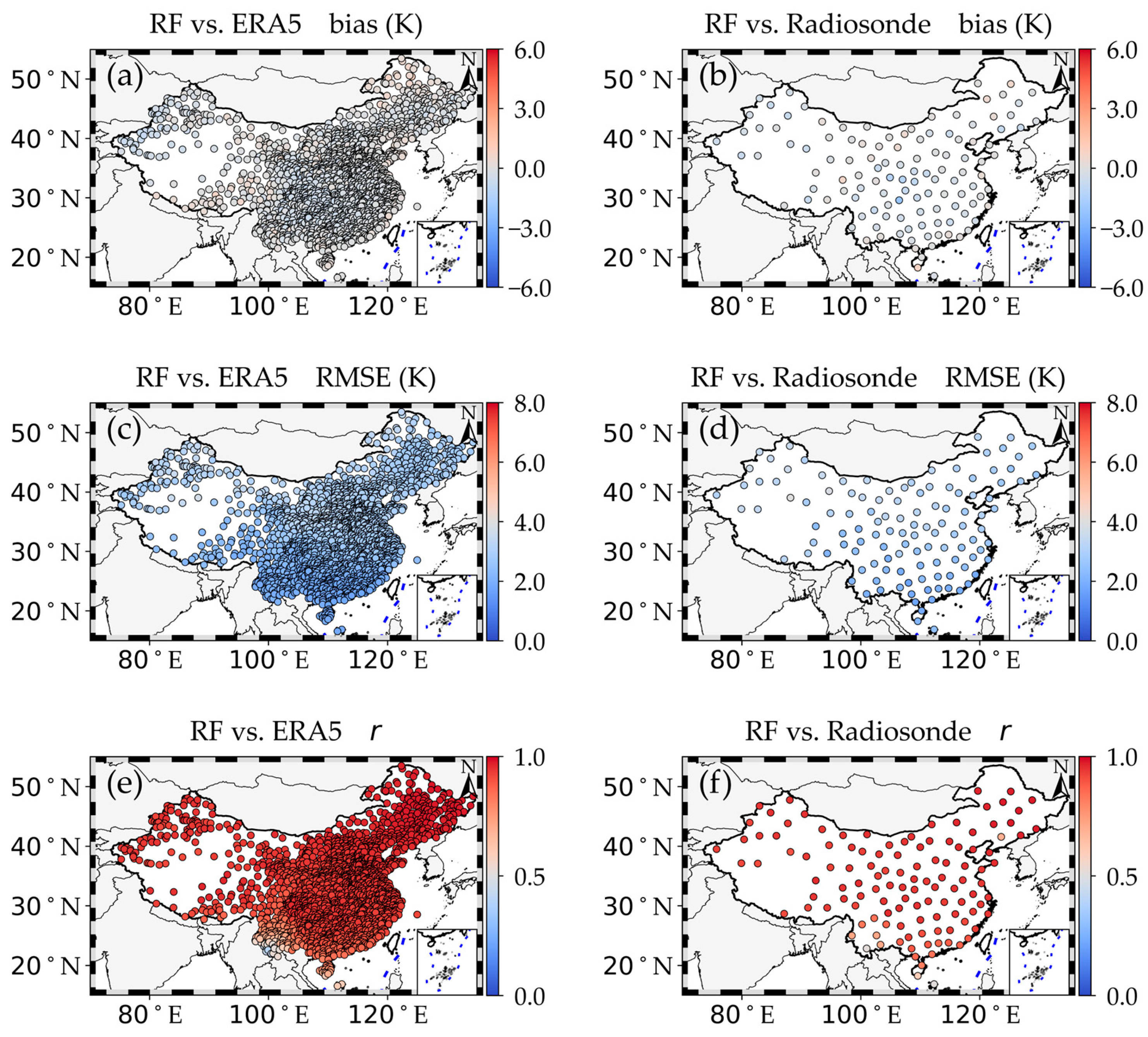
The comparisons of Tm from the RF model with those from ERA5 and radiosonde observations are shown in Figure 8. Compared with the linear Tm model, the accuracy of Tm derived from the RF model is greatly improved. The Tm bias values of the RF model relative to ERA5 across the entire China range from −1.1 K to 1.1 K (Figure 8a). The Tm RMSE values range from 1.7 K to 3.8 K, with higher values in northern China than in southern China (Figure 8c). In most parts of China, the correlation coefficient (r) values are greater than 0.8, except for regions in southwestern China where some stations have r values as low as 0.4 (Figure 8e). Additionally, the Tm bias of the RF model relative to radiosonde observations ranges from −2.1 K to 0.8 K, the Tm RMSE ranges from 1.7 K to 4.0 K, and the r values range from 0.51 to 0.98. Large Tm RMSE values from the RF model occur at stations in the desert regions of northwestern China (Figure 8b,d,f). Therefore, the RF model performs better than the linear model in Tm estimation.

Figure 8. Geographical distribution of the Tm bias of the RF model relative to (a) ERA5 and (b) radiosonde observations, Tm RMSE relative to (c) ERA5 and (d) radiosonde observations, and correlation coefficients between the RF model and (e) ERA5 as well as between the RF model and (f) radiosonde observations over China in 2024.

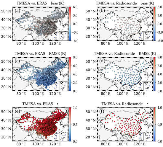
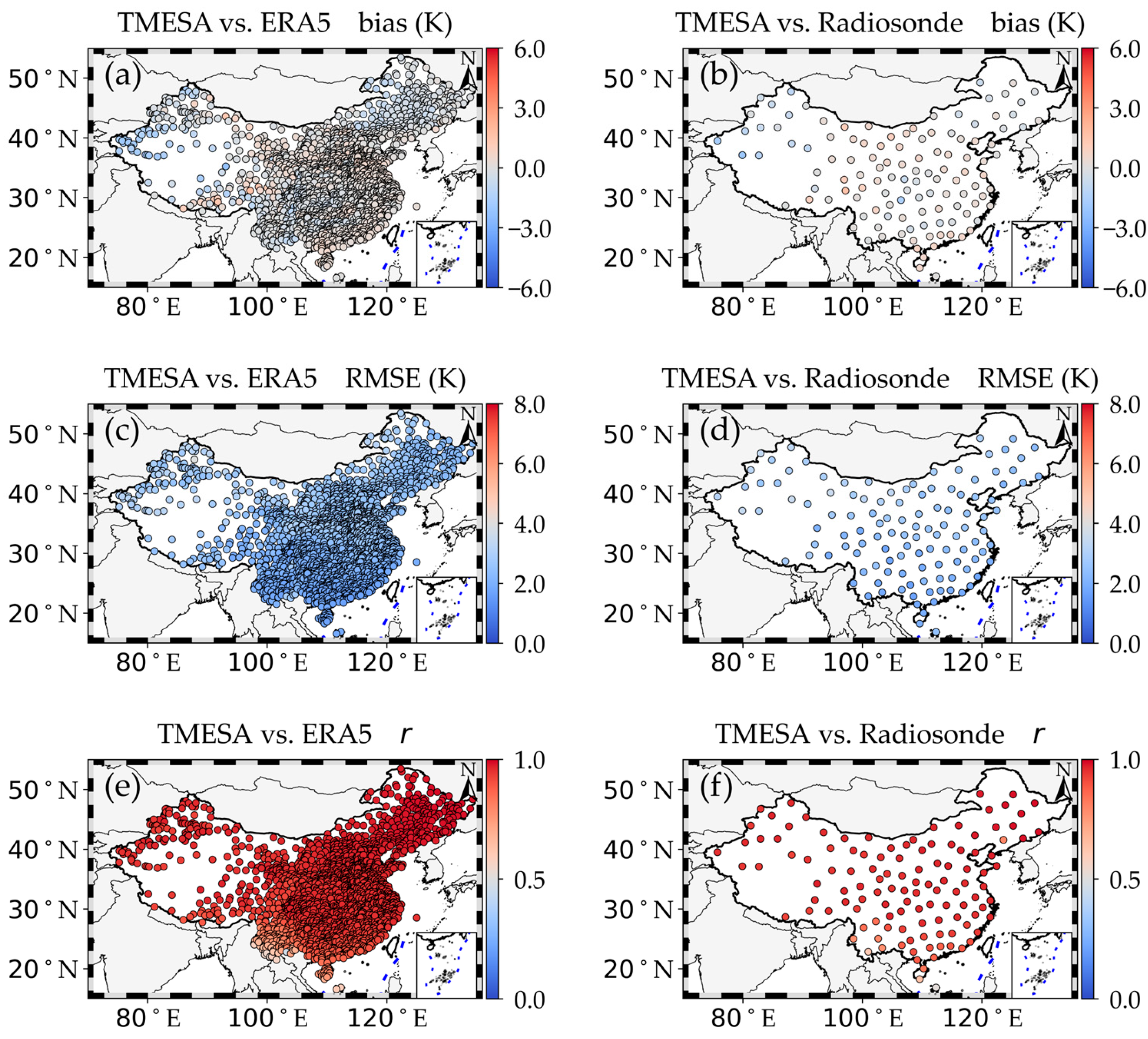
Figure 9 demonstrates the comparisons of Tm from the TMESA model with those from ERA5 and sounding observations. The accuracy of Tm derived from the TMESA model is also significantly improved compared with that from the linear Tm model. The Tm bias values of the TMESA model relative to ERA5 across the entire China range from −2.3 K to 1.9 K (Figure 9a). The Tm RMSE values range from 1.6 K to 4.0 K, with higher values in northern China than in southern China (Figure 9c). In most parts of China, the correlation coefficient (r) values are greater than 0.8, except for regions in southwestern China where some stations have r values as low as 0.46 (Figure 9e). Additionally, the Tm bias of the TMESA model relative to radiosonde observations ranges from −2.0 K to 1.6 K, the Tm RMSE ranges from 1.6 K to 3.6 K, and the r values range from 0.51 to 0.99 (Figure 9b,d,f). Large Tm RMSE values from the TMESA model occur at stations in the desert regions of northwestern China. Therefore, the TMESA model performs much better than the linear model in Tm estimation.

Figure 9. Same as Figure 8 but for TMESA model. Geographical distribution of the Tm bias of the TMESA model relative to (a) ERA5 and (b) radiosonde observations, Tm RMSE relative to (c) ERA5 and (d) radiosonde observations, and correlation coefficients between the TMESA model and (e) ERA5 as well as between the TMESA model and (f) radiosonde observations over China in 2024.

4.2. Model Comparison and Comprehensive Evaluation

The length of the training dataset plays a prominent role in creating a stable Tm model. The Tm modeling performance of the linear, RF, and TMESA models trained with datasets of different time lengths is presented in Table 2. The linear model was constructed using the 10 yr dataset from 2014 to 2023, while the RF and TMESA models were constructed using the 9 yr dataset from 2014 to 2022. The dataset in 2023 was applied to test the RF and TMESA models. Generally, the three models exhibit good Tm modeling performance when the time length of the training data reaches or exceeds 4 years. All these models have small average biases over China, which range from −0.1 K to 0.13 K. Meanwhile, the Tm RMSE values for the linear, RF, and TMESA models are 3.90 K, 2.68 K, and 2.35 K, respectively, when a 7-year dataset is used as the model training input. Furthermore, the r values for Tm modeling by the linear, random forest, and TMESA models are 0.92, 0.96, and 0.97, respectively. Therefore, a 9-year dataset is sufficient to generate Tm models with good performance.

Table 2. Tm modeling performance of the linear, RF, and TMESA models trained with datasets of different time lengths. These models were independently validated using ERA5 reanalysis from 2024.

Total Years	Linear			RF			TMESA
	Bias (K)	RMSE (K)	r	Bias (K)	RMSE (K)	r	Bias (K)	RMSE (K)	r
1	−0.26	3.92	0.92	−0.07	2.93	0.95	−0.11	2.67	0.96
2	−0.09	3.90	0.92	−0.09	2.84	0.96	−0.24	2.54	0.97
3	−0.03	3.90	0.92	−0.11	2.79	0.96	−0.12	2.50	0.97
4	0.04	3.90	0.92	−0.11	2.75	0.96	0.10	2.42	0.97
5	0.08	3.90	0.92	−0.11	2.75	0.96	0.03	2.39	0.97
6	0.08	3.90	0.92	−0.12	2.73	0.96	0.09	2.35	0.97
7	0.10	3.90	0.92	−0.10	2.68	0.96	−0.05	2.33	0.97
8	0.11	3.90	0.92	−0.10	2.68	0.96	−0.09	2.35	0.97
9	0.13	3.90	0.92	−0.11	2.67	0.96	−0.02	2.34	0.97
10	0.13	3.90	0.92	/	/	/	/	/	/

The “/” means no data.

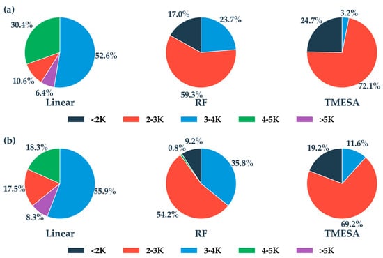
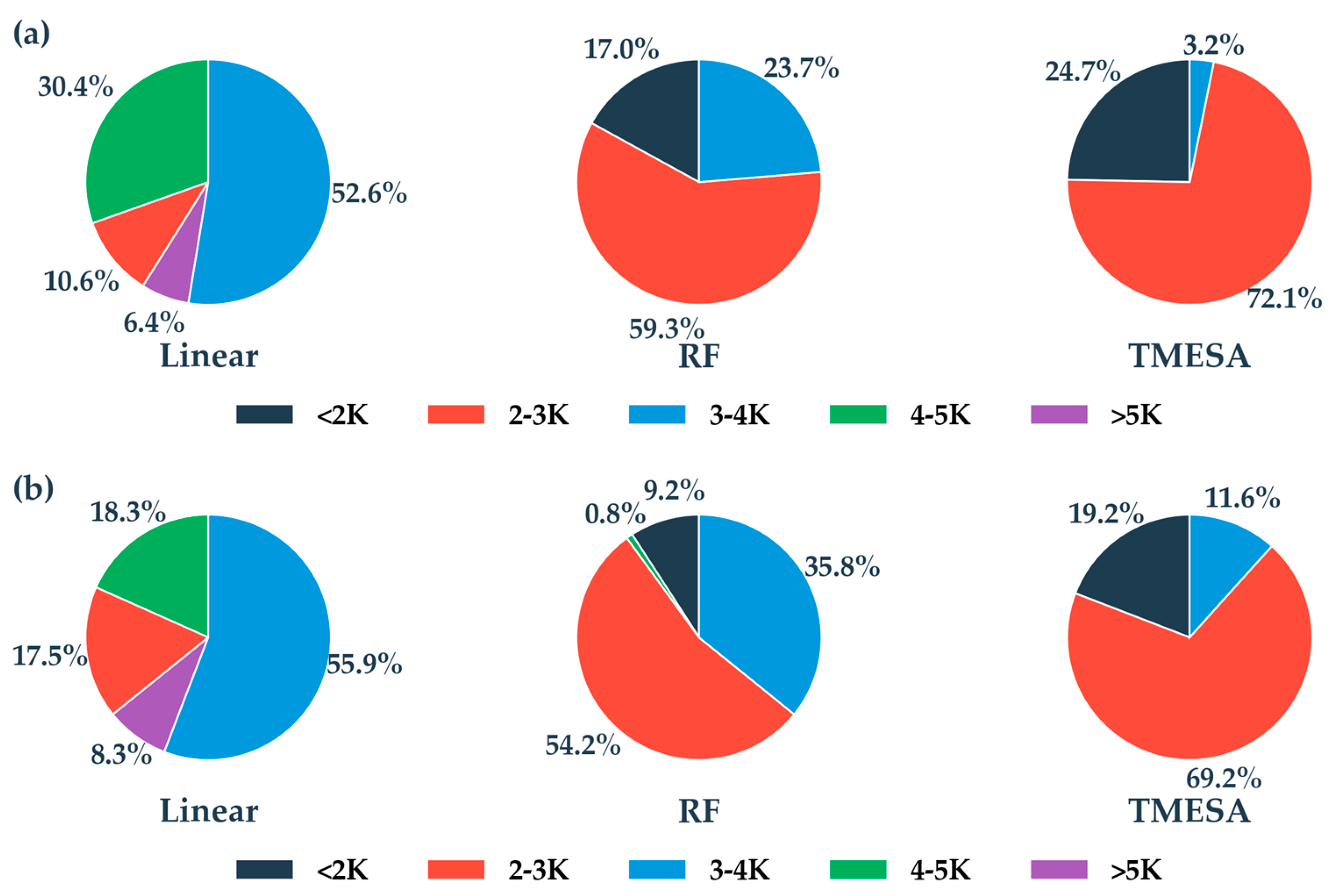
The proportion distributions of Tm RMSE from the linear, RF and TMESA models compared with ERA5 and radiosonde observations are presented in Figure 10. When compared with ERA5 (Figure 10a), the proportions of Tm RMSE less than 2 K for the linear, RF, and TMESA models are 0%, 17.0%, and 24.7%, respectively. Meanwhile, the percentages of Tm RMSE between 2 and 3 K for these three models are 10.6%, 59.3%, and 72.1%, respectively. In total, the proportions of Tm RMSE less than 3 K for the three models are 10.6%, 76.3%, and 96.8%, respectively. When compared with radiosonde observations, the percentages of Tm RMSE less than 2 K for the linear, RF, and TMESA models are 0%, 9.2%, and 19.2%, respectively. Additionally, the percentages of Tm RMSE between 2 and 3 K for these three models are 17.5%, 54.2%, and 69.2%, respectively. Overall, the proportions of Tm RMSE less than 3 K from the three models are 17.5%, 63.4%, and 88.4%, respectively. If model output with Tm RMSE less than 3 K is considered to be of good performance, as demonstrated by Zhao et al. [17] and Huang et al. [19], both the RF and TMESA models greatly improve Tm modeling accuracy over China, with the TMESA model performing better than the RF model.

Figure 10. The pie chart of percentages for Tm RMSE from linear, RF and TMESA models compared with ERA5 (a) and radiosonde observations (b) in 2024.

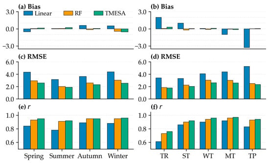
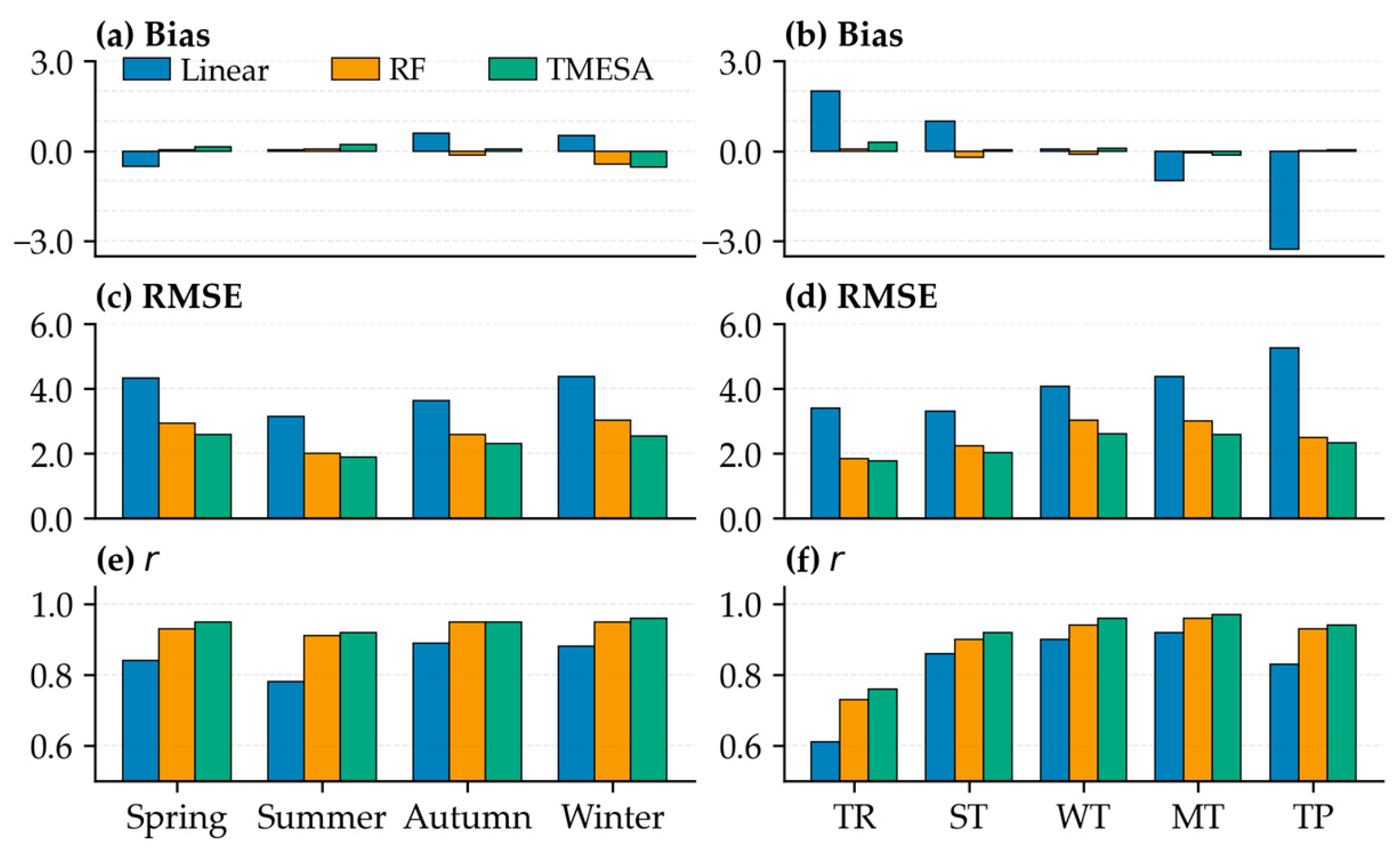
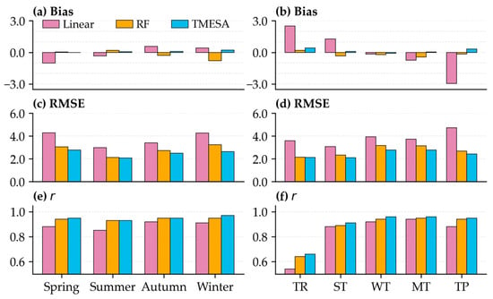
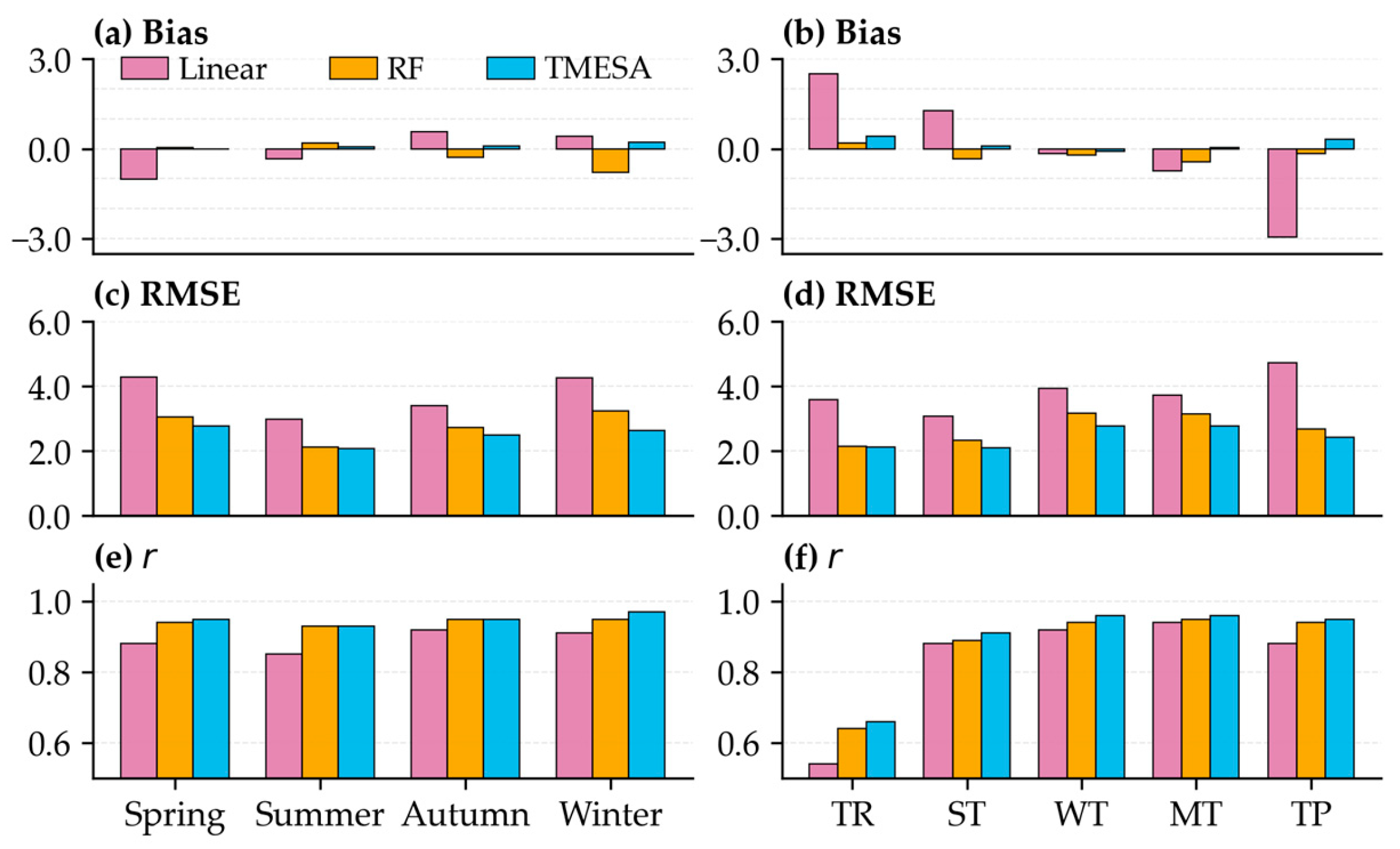
The characteristics of Tm bias and RMSE compared with ERA5, as well as the correlation coefficients between different Tm models and ERA5 across various seasons and climate zones in China, are shown in Figure 11. The mean Tm bias values are almost between −0.5 and 0.5 K, except for the linear model, whose mean Tm bias is 2.0 K in the tropical climate zone and −3.3 K over the Tibetan Plateau. Basically, the mean Tm biases for the linear model, RF model, and TMESA model over China in 2024 are 0.13 K, −0.11 K, and −0.02 K, respectively. In addition, the linear model exhibits the largest Tm RMSE among the three models across all seasons and climate zones, with the maximum Tm RMSE of 5.3 K observed over the Tibetan Plateau. In contrast, the TMESA model has the smallest Tm RMSE across all seasons and climate zones. All models achieve the smallest Tm RMSE in summer. The mean Tm RMSE values for the linear model, RF model, and TMESA model over China in 2024 are 3.90 K, 2.67 K, and 2.34 K, respectively. Furthermore, the TMESA model achieves the highest correlation coefficients across different seasons and climate zones, which are almost all greater than 0.9 except in the tropical climate zone, where the correlation coefficients for all three models are less than 0.8. The consistent high r values (>0.9) of RF and TMESA indicate their robust capability to capture Tm temporal variability regardless of seasonal or climatic differences. Figure 12 demonstrates the Tm errors for linear, RF and TMESA models validated against sounding observations. The mean Tm biases for the linear model, RF model, and TMESA model over China in 2024 are −0.1 K, −0.21 K, and 0.09 K, respectively, and the mean Tm RMSE values are 3.66 K, 2.67 K, and 2.46 K, respectively.

Figure 11. The bias, RMSE and correlation coefficient (r) for linear, RF and TMESA models compared with ERA5 across different seasons (a,c,e) and climate zones (b,d,f).

Figure 12. The bias, RMSE and correlation coefficient (r) for linear, RF and TMESA models compared with radiosonde observations across different seasons (a,c,e) and climate zones (b,d,f).

The linear model also yields substantial Tm biases across tropical climatic zones and the Tibetan Plateau, indicating its inability to characterize the Tm–Ts relationship in these two regions. In contrast, it exhibits modest seasonal mean Tm biases against ERA5 and radiosonde measurements (Figure 11 and Figure 12). This discrepancy likely originates from offsetting errors, namely positive Tm bias prevails in tropical zones, whereas negative bias dominates over the Tibetan Plateau. Consequently, the nationally averaged seasonal mean Tm bias of the linear model remains low after nationwide aggregation across China. Across all five climatic zones—tropical (TR), subtropical (ST), warm temperate (WT), mid-temperate (MT), and Tibetan Plateau (TP)—the RF and TMESA models produce Tm RMSE ranging from 2 to 3 K. Although slightly higher Tm RMSE is found for RF and TMESA in WT and MT compared with TR, ST, and TP, both models effectively capture the nonlinear dependencies between Tm and near-surface meteorological variables, including surface air temperature, pressure, relative humidity, and other relevant predictors over China. Further research is required to elucidate why the Tm RMSE values in WT and MT are marginally higher than those in TR, ST and TP. In general, our RF Tm model is comparable to that presented by Huang [19] using the same method, which had a mean RMSE of 2.47 K and a mean bias of −0.38 K validating against sounding observations in China. Furthermore, Ding [9] developed a neural network model for Tm estimation, which yielded a mean RMSE of 3.34 K and a mean bias of 0.08 K when compared with radiosonde observations. A long short-term memory (LSTM)-based model for Tm determination had a mean Tm RMSE of 4.2 K and a mean bias of 0.65 K when validated with sounding data and a mean Tm RMSE of 3.16 K and a mean bias of −0.15 K when evaluated against ERA5 [17]. Therefore, the TMESA model in this study significantly improves Tm estimation accuracy for China.

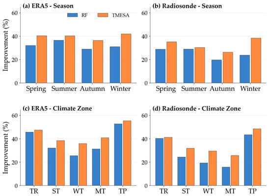
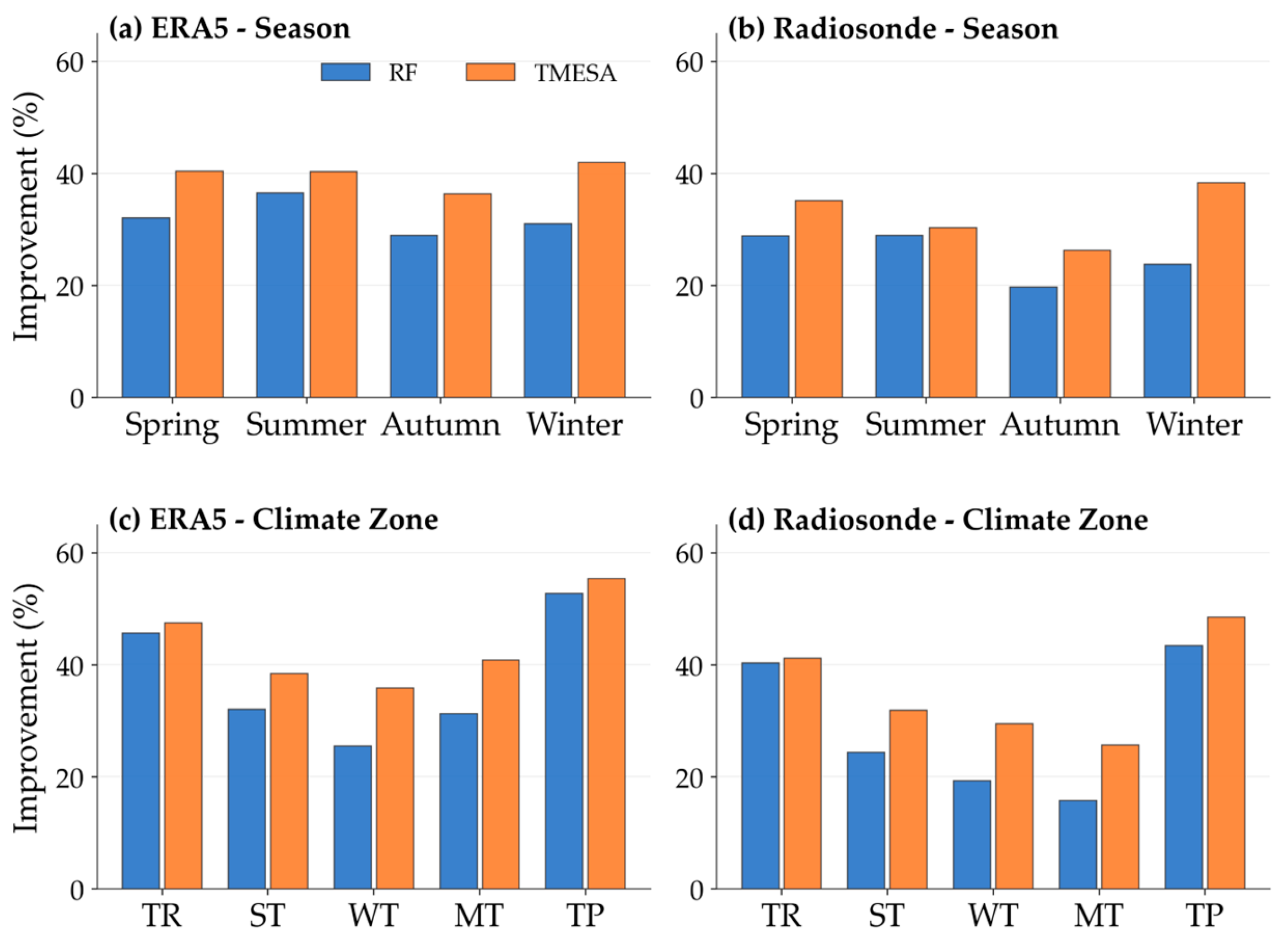
Compared with the linear model, the Tm modeling performance of the RF model is improved by 32%, 37%, 29%, and 31% in spring, summer, autumn, and winter, respectively, when validated against ERA5 reanalysis (Figure 13a). For the TMESA model, the corresponding improvements are 40%, 40%, 36%, and 42%, respectively. Additionally, the Tm modeling performance of the RF model is improved by 46%, 32%, 26%, 31%, and 53% in the tropical zone (TR), subtropical zone (ST), warm temperate zone (WT), mid-temperate zone (MT), and Tibetan Plateau (TP), respectively (Figure 13c). For the TMESA model, the corresponding improvements are 47%, 38%, 36%, 41%, and 55%, respectively. Meanwhile, when validated against radiosonde observations, the Tm modeling performance of the RF model is improved by 29%, 29%, 20%, and 24% in spring, summer, autumn, and winter, respectively (Figure 13b). For the TMESA model, the corresponding improvements are 35%, 30%, 26%, and 38%, respectively. Additionally, the Tm modeling performance of the RF model is improved by 40%, 24%, 19%, 16%, and 43% in TR, ST, WT, MT, and TP, respectively. The TMESA model achieves even greater improvements in these climate zones, with increases of 41%, 32%, 30%, 26%, and 49%, respectively. In general, the average Tm modeling performance of the RF model is improved by 32% and 25%, respectively, when validated against ERA5 and sounding observations. For the TMESA model, the average improvements are 40% and 33%, respectively, when validated against ERA5 and radiosonde observations.

Figure 13. The improvement of Tm modeling by RF model and TMESA model compared with linear model.

5. Discussion

Accurate estimates of atmospheric weighted mean temperature (Tm) are crucial for the calculation of precipitable water vapor (PWV) derived from ground-based GNSS observations. Machine learning represents an effective approach for capturing the nonlinear relationships between Tm time series, station geographical coordinates, and surface meteorological parameters. Recent studies [9,17,19] have shown that neural network and machine learning models yield superior Tm modeling performance compared with traditional linear models [7]. However, surface meteorological observations at GNSS-equipped stations warrant in-depth investigation to fully exploit their potential in retrieving high-precision Tm estimates. We constructed two Tm models based on the RF and TMESA algorithms, incorporating meteorological station observations of pressure, relative humidity and temperature alongside periodic and geographic covariates. The results of this study indicate that the accuracy of Tm estimates from both RF and TMESA were greatly improved compared with the traditional linear model. These improvements demonstrate the capability of machine learning methods to capture complex nonlinear relationships in atmospheric thermodynamics.

In terms of computational efficiency, the linear empirical model involves only elementary algebraic calculations. The linear model training finishes in roughly 5 min, while the full prediction for the 2024 dataset (over 20.6 million samples from 2377 stations) takes merely 1 min. In contrast, RF and TMESA involve more complex training processes. However, once trained, both models achieve relatively high prediction efficiency, with RF requiring 5 min and TMESA 7 min for the 2024 dataset. This “high training cost, low prediction cost” characteristic is suitable for operational applications where models are trained offline and then deployed. The trade-off between significantly improved accuracy (Tm RMSE reduced by 32–40% against ERA5) and moderately increased prediction time is favorable for applications requiring high-precision Tm estimates.

It should be noted that the proposed Tm models require surface meteorological observations (air temperature, pressure, and relative humidity) as input features, which may limit their application at GNSS stations without co-located meteorological sensors. However, GNSS stations constructed by the China Meteorological Administration (CMA) are all equipped with corresponding meteorological instruments. The collocated surface air pressure, temperature and relative humidity measurements can be used as RF and TMESA models input to obtain Tm estimates. Additionally, the China Meteorological Administration (CMA) currently operates over 10,000 meteorological stations instrumented with sensors for air temperature, atmospheric pressure and relative humidity. While GNSS stations operated by external agencies may lack collocated meteorological sensors, most are situated in close proximity to meteorological sites, permitting direct implementation of the proposed models. For GNSS sites suffering from incomplete or missing hourly meteorological observations, three gap-filling schemes are available, which are temporal interpolation for brief data lapses, spatial interpolation using adjacent station records to address prolonged outages, and reanalysis datasets as an alternative backup approach.

6. Conclusions

In this study, we develop regional empirical models for Tm using random forest (RF) and Temporal Mixture of Experts with Sequential Attention (TMESA), aiming to provide more reliable real-time Tm estimates and thereby improve the accuracy of operational PWV retrievals over China. A conventional linear model is employed as a baseline to quantify improvements in Tm modeling achieved by the RF and TMESA approaches. The model were trained and tested using hourly Tm retrievals derived from ERA5 reanalysis, along with in situ measurements of pressure, temperature, and relative humidity from meteorological stations across the 10-year period from 2014 to 2023. Diurnal variations in Tm, station geographic coordinates, day of year, year, month, and day are also incorporated as predictive features. The radiosonde profiles from 120 stations and ERA5 in 2024 over China were used to validate the Tm models. Totally, there are 177,139,624 data samples for training the machine learning models, 20,577,501 data samples for model testing, and 20,609,231 data samples and 87,600 radiosonde profiles for model validations.

The results indicate that the RF model yields a bias (RMSE) of −0.11 K (2.67 K) against ERA5 and −0.21 K (2.67 K) against radiosonde profiles. The TMESA model achieves even better performance, with a bias (RMSE) of −0.02 K (2.34 K) relative to ERA5 and 0.09 K (2.46 K) relative to radiosonde measurements. The accuracy of Tm estimates from both RF and TMESA is comparable to that reported in the recent literature [17,19]. Compared with the traditional linear model, the RF model reduces Tm RMSE by 32% against ERA5 and 25% against radiosonde data, while the TMESA model achieves reductions of 40% and 33%, respectively. These results demonstrate that the proposed machine learning methods can supply high-precision Tm estimates to support GNSS-based PWV retrieval.

As a critical parameter for ground-based GNSS-PWV retrieval, the Tm derived herein merits further experimental investigations into PWV estimation at representative GNSS sites. This work is out of the scope of this study. In future work, we will focus on further verifying the reliability of Tm on enhancing GNSS-PWV inversion and the operational implementation of these machine learning models for near-real-time GNSS-based PWV estimation.

References

- Gimeno, L.; Vázquez, M.; Eiras-Barca, J.; Sorí, R.; Stojanovic, M.; Algarra, I.; Nieto, R.; Ramos, A.M.; Durán-Quesada, A.M.; Domínguez, F. Recent Progress on the Sources of Continental Precipitation as Revealed by Moisture Transport Analysis. Earth-Sci. Rev. 2020, 201, 103070. [Google Scholar] [CrossRef] [Scilit]
- Guerova, G.; Jones, J.; Douša, J.; Dick, G.; De Haan, S.; Pottiaux, E.; Bock, O.; Pacione, R.; Elgered, G.; Vedel, H.; et al. Review of the State of the Art and Future Prospects of the Ground-Based GNSS Meteorology in Europe. Atmos. Meas. Tech. 2016, 9, 5385–5406. [Google Scholar] [CrossRef] [Scilit]
- Guerreiro, S.B.; Fowler, H.J.; Barbero, R.; Westra, S.; Lenderink, G.; Blenkinsop, S.; Lewis, E.; Li, X.-F. Detection of Continental-Scale Intensification of Hourly Rainfall Extremes. Nat. Clim. Change 2018, 8, 803–807. [Google Scholar] [CrossRef] [Scilit]
- Neelin, J.D.; Martínez-Villalobos, C.; Stechmann, S.N.; Ahmed, F.; Chen, G.; Norris, J.M.; Kuo, Y.-H.; Lenderink, G. Precipitation Extremes and Water Vapor: Relationships in Current Climate and Implications for Climate Change. Curr. Clim. Change Rep. 2022, 8, 17–33. [Google Scholar] [CrossRef] [Scilit]
- Douville, H.; Raghavan, K.; Renwick, J.; Allan, R.P.; Arias, P.A.; Barlow, M.; Cerezo-Mota, R.; Cherchi, A.; Gan, T.; Gergis, J.; et al. Water Cycle Changes. In Climate Change 2021: The Physical Science Basis. Contribution of Working Group I to the Sixth Assessment Report of the Intergovernmental Panel on Climate Change; Masson-Delmotte, V., Zhai, P., Pirani, A., Connors, S.L., Péan, C., Berger, S., Caud, N., Chen, Y., Goldfarb, L., Gomis, M.I., et al., Eds.; Cambridge University Press: Cambridge, UK; New York, NY, USA, 2021; pp. 1055–1210. [Google Scholar]
- Jones, J.; Guerova, G.; Douša, J.; Dick, G.; De Haan, S.; Pottiaux, E.; Bock, O.; Pacione, R.; Van Malderen, R. Advanced GNSS Tropospheric Products for Monitoring Severe Weather Events and Climate; COST Action ES1206 Final Action Dissemination Report; Springer International Publishing: Cham, Switzerland, 2020; p. 577. [Google Scholar]
- Bevis, M.; Businger, S.; Herring, T.A.; Rocken, C.; Anthes, R.A.; Ware, R.H. GPS Meteorology: Remote Sensing of Atmospheric Water Vapor Using the Global Positioning System. J. Geophys. Res. 1992, 97, 15787–15801. [Google Scholar] [CrossRef] [Scilit]
- Wang, J.; Zhang, L.; Dai, A. Global Estimates of Water-Vapor-Weighted Mean Temperature of the Atmosphere for GPS Applications. J. Geophys. Res. Atmos. 2005, 110, D21101. [Google Scholar] [CrossRef] [Scilit]
- Ding, M. A Second Generation of the Neural Network Model for Predicting Weighted Mean Temperature. GPS Solut. 2020, 24, 61. [Google Scholar] [CrossRef] [Scilit]
- Sun, Z.; Zhang, B.; Yao, Y. A Global Model for Estimating Tropospheric Delay and Weighted Mean Temperature Developed with Atmospheric Reanalysis Data from 1979 to 2017. Remote Sens. 2019, 11, 1893. [Google Scholar] [CrossRef] [Scilit]
- Ding, M. A Neural Network Model for Predicting Weighted Mean Temperature. J. Geod. 2018, 92, 1187–1198. [Google Scholar] [CrossRef] [Scilit]
- Cai, M.; Li, J.; Liu, L.; Huang, L.; Zhou, L.; Huang, L.; He, H. Weighted Mean Temperature Hybrid Models in China Based on Artificial Neural Network Methods. Remote Sens. 2022, 14, 3762. [Google Scholar] [CrossRef] [Scilit]
- Li, K.; Li, L.; Hu, A.; Pan, J.; Ma, Y.; Zhang, M. Research on Modeling Weighted Average Temperature Based on the Machine Learning Algorithms. Atmosphere 2023, 14, 1251. [Google Scholar] [CrossRef] [Scilit]
- Zhu, M.; Yu, X.; Sun, W. A Coalescent Grid Model of Weighted Mean Temperature for China Region Based on Feedforward Neural Network Algorithm. GPS Solut. 2022, 26, 70. [Google Scholar] [CrossRef] [Scilit]
- Landskron, D.; Böhm, J. VMF3/GPT3: Refined Discrete and Empirical Troposphere Mapping Functions. J. Geod. 2018, 92, 349–360. [Google Scholar] [CrossRef] [Scilit] [PubMed]
- Sun, Z.; Zhang, B.; Yao, Y. An ERA5-Based Model for Estimating Tropospheric Delay and Weighted Mean Temperature Over China with Improved Spatiotemporal Resolutions. Earth Space Sci. 2019, 6, 1926–1941. [Google Scholar] [CrossRef] [Scilit]
- Zhao, X.; Niu, Q.; Chi, Q.; Chen, J.; Liu, C. A New LSTM-Based Model to Determine the Atmospheric Weighted Mean Temperature in GNSS PWV Retrieval. GPS Solut. 2024, 28, 74. [Google Scholar]
- Collins, J.; Langley, R. A Tropospheric Delay Model for the User of the Wide Area Augmentation System; Nav Canada: Fredericton, NB, Canada, 1997. [Google Scholar]
- Huang, L.; Wang, Y.; Bi, H.; Zhu, G.; Liu, L.; Jiang, W. Initial Results of Atmospheric Weighted Mean Temperature Estimation with Pangu-Weather in Real-Time GNSS PWV Retrieval for China. GPS Solut. 2025, 29, 48. [Google Scholar] [CrossRef] [Scilit]
- Ma, Y.; Chen, P.; Liu, T.; Xu, G.; Lu, Z. Development and Assessment of an ALLSSA-Based Atmospheric Weighted Mean Temperature Model with High Time Resolution for GNSS Precipitable Water Retrieval. Earth Space Sci. 2022, 9, e2021EA002089. [Google Scholar] [CrossRef] [Scilit]
- Yao, Y.; Zhu, S.; Yue, S. A Globally Applicable, Season-Specific Model for Estimating the Weighted Mean Temperature of the Atmosphere. J. Geod. 2012, 86, 1125–1135. [Google Scholar] [CrossRef] [Scilit]
- Yao, Y.; Zhang, B.; Yue, S.; Xu, C.; Peng, W. Global Empirical Model for Mapping Zenith Wet Delays onto Precipitable Water. J. Geod. 2013, 87, 439–448. [Google Scholar] [CrossRef] [Scilit]
- Yang, F.; Wang, L.; Li, Z.; Tang, W.; Meng, X. A Weighted Mean Temperature (Tm) Augmentation Method Based on Global Latitude Zone. GPS Solut. 2022, 26, 141. [Google Scholar] [CrossRef] [Scilit]
- Böhm, J.; Möller, G.; Schindelegger, M.; Pain, G.; Weber, R. Development of an Improved Empirical Model for Slant Delays in the Troposphere (GPT2w). GPS Solut. 2015, 19, 433–441. [Google Scholar] [CrossRef] [Scilit]
- Chen, P.; Yao, W.; Zhu, X. Realization of Global Empirical Model for Mapping Zenith Wet Delays onto Precipitable Water Using NCEP Re-Analysis Data. Geophys. J. Int. 2014, 198, 1748–1757. [Google Scholar] [CrossRef] [Scilit]
- He, C.; Wu, S.; Wang, X.; Hu, A.; Wang, Q.; Zhang, K. A New Voxel-Based Model for the Determination of Atmospheric Weighted Mean Temperature in GPS Atmospheric Sounding. Atmos. Meas. Tech. 2017, 10, 2045–2060. [Google Scholar] [CrossRef] [Scilit]
- Huang, L.; Jiang, W.; Liu, L.; Chen, H.; Ye, S. A New Global Grid Model for the Determination of Atmospheric Weighted Mean Temperature in GPS Precipitable Water Vapor. J. Geod. 2019, 93, 159–176. [Google Scholar] [CrossRef] [Scilit]
- Yao, Y.; Zhang, B.; Xu, C.; Yan, F. Improved One/Multi-Parameter Models That Consider Seasonal and Geographic Variations for Estimating Weighted Mean Temperature in Ground-Based GPS Meteorology. J. Geod. 2014, 88, 273–282. [Google Scholar] [CrossRef] [Scilit]
- Zhang, J.; Yang, L.; Wang, J.; Wang, Y.; Liu, X. A New Empirical Model of Weighted Mean Temperature Combining ERA5 Reanalysis Data, Radiosonde Data, and TanDEM-X 90m Products over China. Remote Sens. 2024, 16, 855. [Google Scholar] [CrossRef] [Scilit]
- Zhang, B.; Wu, T.; Shen, Y. Atmospheric Weighted Average Temperature Enhancement Model for the European Region Considering Daily Variations and Residual Changes in Surface Temperature. Remote Sens. 2026, 18, 36. [Google Scholar] [CrossRef] [Scilit]
- Hersbach, H.; Bell, B.; Berrisford, P.; Biavati, G.; Horányi, A.; Muñoz Sabater, J.; Nicolas, J.; Peubey, C.; Radu, R.; Rozum, I.; et al. ERA5 Hourly Data on Pressure Levels from 1940 to Present. Copernicus Climate Change Service (C3S) Climate Data Store (CDS). Available online: https://cds.climate.copernicus.eu/datasets/reanalysis-era5-pressure-levels?tab=overview (accessed on 1 January 2025).
- Zhang, W.; Zhang, H.; Liang, H.; Lou, Y.; Cai, Y.; Cao, Y.; Zhou, Y.; Liu, W. On the Suitability of ERA5 in Hourly GPS Precipitable Water Vapor Retrieval Over China. J. Geod. 2019, 93, 1897–1909. [Google Scholar] [CrossRef] [Scilit]
- Sun, Y.; Yang, F.; Liu, M.; Li, Z.; Gong, X.; Wang, Y. Evaluation of the Weighted Mean Temperature Over China Using Multiple Reanalysis Data and Radiosonde. Atmos. Res. 2023, 285, 106664. [Google Scholar] [CrossRef] [Scilit]
- Davis, J.L.; Herring, T.A.; Shapiro, I.I.; Rogers, A.E.E.; Elgered, G. Geodesy by Radio Interferometry: Effects of Atmospheric Modeling Errors on Estimates of Baseline Length. Radio Sci. 1985, 20, 1593–1607. [Google Scholar] [CrossRef] [Scilit]
- Ho, T.K. Random Decision Forests. In Proceedings of the 3rd International Conference on Document Analysis and Recognition, Montreal, QC, Canada, 14–16 August 1995; IEEE Computer Society: Washington, DC, USA, 1995; Volume 1, pp. 278–282. [Google Scholar]
- Tyralis, H.; Papacharalampous, G.; Langousis, A. A Brief Review of Random Forests for Water Scientists and Practitioners and Their Recent History in Water Resources. Water 2019, 11, 910. [Google Scholar] [CrossRef] [Scilit]
- Jacobs, R.A.; Jordan, M.I.; Nowlan, S.J.; Hinton, G.E. Adaptive Mixtures of Local Experts. Neural Comput. 1991, 3, 79–87. [Google Scholar] [CrossRef] [Scilit]
- Shazeer, N.; Mirhoseini, A.; Maziarz, K.; Davis, A.; Le, Q.; Hinton, G.; Dean, J. Outrageously Large Neural Networks: The Sparsely-Gated Mixture-of-Experts Layer. In Proceedings of the International Conference on Learning Representations (ICLR), Toulon, France, 24–26 April 2017. [Google Scholar]
- Fedus, W.; Zoph, B.; Shazeer, N. Switch Transformers: Scaling to Trillion Parameter Models with Simple and Efficient Sparsity. J. Mach. Learn. Res. 2022, 23, 5232. [Google Scholar]
- Lundberg, S.M.; Lee, S.-I. A Unified Approach to Interpreting Model Predictions. In Proceedings of the 31st Conference on Neural Information Processing Systems (NIPS 2017), Long Beach, CA, USA, 4–9 December 2017; pp. 4765–4774. [Google Scholar]
- Yao, Y.; Zhang, B.; Xu, C.; Chen, J. Analysis of the Global Tm–Ts Correlation and Establishment of the Latitude-Related Linear Model. Chin. Sci. Bull. 2014, 59, 2340–2347. [Google Scholar] [CrossRef] [Scilit]
Disclaimer/Publisher’s Note: The statements, opinions and data contained in all publications are solely those of the individual author(s) and contributor(s) and not of MDPI and/or the editor(s). MDPI and/or the editor(s) disclaim responsibility for any injury to people or property resulting from any ideas, methods, instructions or products referred to in the content. |
© 2026 by the authors. Licensee MDPI, Basel, Switzerland. This article is an open access article distributed under the terms and conditions of the Creative Commons Attribution (CC BY) license.