


Highlights
What are the main findings?
- Addressing the “Saturation Problem” in ExistingWide-Area Maps and High-Biomass Regions.
- The importance of AGB estimation using methods that consider Japan’s regional characteristics and tree species.
What is the implication of the main finding?
- In Japanese forests, estimates tended to saturate at approximately 300–400 Mg/ha, leading to a significant underestimation of high-biomass areas. Global biomass maps (such as ESA CCI) exhibit a similar trend. This study ensures consistency and robustness against saturation, even in high AGB (Above-Ground Biomass) regions, by adopting a hybrid approach that combines tree height estimation with forest-type-specific allometric equations, rather than relying solely on machine learning. We demonstrated that accuracy can be maintained in high-biomass areas, reproducing an AGBD distribution close to actual measurements.
- To account for Japan’s complex topography and diverse tree species (e.g., mixed evergreen/deciduous and needleleaf/broadleaf forests), we achieved improved accuracy by using optimized parameters for each forest type instead of a uniform national model. This high-precision, 10m-resolution national map enables precise carbon sink assessments reflecting regional differences in forest structure. It will serve as highly practical foundational information for transparent carbon credit trading and the formulation of municipal-level forest management plans.
Abstract
Continuous monitoring of forest biomass is indispensable for establishing transparent carbon budgets and ensuring sustainable forest management toward achieving carbon neutrality. While satellite data has traditionally been used for wide-area biomass estimation, signal saturation in high-biomass regions has posed a significant challenge to accuracy. To address this saturation issue and enhance the precision of carbon budget estimations, this study develops a new methodology for estimating forest above-ground biomass (AGB). First, a training dataset was constructed by integrating airborne LiDAR data from across Japan with various satellite datasets, such as PALSAR-2 and Sentinel-2. Machine learning (XGBoost) was then employed to generate a nationwide canopy height map, achieving a high coefficient of determination (). Subsequently, allometric equations with parameters optimized for specific forest types (evergreen coniferous, evergreen broadleaf, deciduous coniferous, and deciduous broadleaf) were derived from the relationship between estimated canopy height and AGB to create a nationwide AGB map. Validation results indicated that the resulting AGB map demonstrated higher estimation accuracy () compared to existing global products (ESA CCI Biomass), with significant improvements in mitigating underestimation (saturation) in high-biomass areas. By combining canopy height estimation with forest-type-specific allometry, this approach enables high-precision mapping that reflects the unique characteristics of Japanese forests and is expected to contribute to more reliable carbon budget assessments.
1. Introduction
Forest biomass that quantifies the impact of land changes caused by logging, fires, and reforestation, as well as the carbon stocks stored in forests, is important for achieving the Paris Agreement’s greenhouse gas reduction targets. Furthermore, with the expansion of REDD+ and carbon credit markets, reliable biomass calculation methods have become a prerequisite for international financing and policy evaluation in many regions, including developing countries [1].
Satellite data is effective because it enables large-scale and consistent observation, allowing for the assessment of biomass distribution across entire countries or globally, which is difficult to achieve through ground surveys. Furthermore, repeated observations enable the tracking of forest changes over time, making it suitable for monitoring land use changes such as logging and afforestation. By combining multiple sensors such as optical, synthetic aperture radar (SAR), and Light Detection and Ranging (LiDAR), it is possible to capture forest structure, such as canopy condition and canopy height, from multiple angles, which is effective for high-precision estimations [2,3]. For these reasons, high-precision forest biomass estimation methods combining satellite data such as optical, SAR, and LiDAR with machine learning are being developed.
GEDI, a representative space-borne LiDAR mounted on the International Space Station (ISS), presents a statistical design that simultaneously estimates the above-ground biomass (AGB) and standard error that is 20% of the mean AGBD on a mesh of approximately 1 km using a 25 m footprint waveform and ground plots and demonstrates a framework that can consistently evaluate the uncertainty of forest carbon monitoring [4]. Numerous studies have shown that Relative Height (RH) percentiles derived from GEDI, such as RH100 (maximum canopy height) and RH50 (height of median energy), function as the most powerful explanatory variables in biomass estimation [5].
Additionally, the Biomass mapping project under the Climate Change Initiative (CCI) conducted by the European Space Agency (ESA) has provided a global AGB map for eight epochs of 2010 and then every year from 2015 to 2021 with 100m resolution by semi-learning modeling the backscatter of ESA’s C-band (Sentinel-1A and B) and JAXA’s L-band (ALOS-2 PALSAR-2) SAR and performing bias correction using GEDI data. While the ability to update annually without dependence on cloud cover is a major advantage, the study also quantified the unique challenge of high-density forests, where the backscattering coefficient saturates and shifts to underestimation around 300 Mg/ha [6,7,8].
Furthermore, the Copernicus Global Land Service (CGLS) has provided dynamic land cover maps (CGLS-LC100) at 100-meter resolution from 2015 to 2019. Information on land cover types and tree cover fraction functions as crucial auxiliary data for large-scale biomass estimation, contributing to the stratification and refinement of estimation models [9]. In region-specific biomass estimation, machine learning leveraging the complementarity of optical and SAR data has been used, achieving values of 0.60–0.71 and RMSE values of 80–105 Mg/ha in Indian tropical forests using Sentinel-1/2 + Random Forest (RF)/GBDT [10]. Additionally, in Botswana’s dry forests, RF tailored to low-AGB areas achieved extremely high accuracy, with 0.95 and RMSE 0.25 Mg/ha [11]. To mitigate SAR observation angle dependence and seasonal noise, a time series analysis averaging 46 PALSAR-2 scenes over more than 10 years in Borneo improved cross-validation error by 15–20% compared to single-period analysis [12]. Furthermore, a two-stage model was used that trains Sentinel-1/2 with ICESat-2 canopy height as the teacher signal using RF learning in inland China [13]. Furthermore, the methodology goes beyond single machine learning models by employing decision tree-based ensemble learning techniques such as XGBoost, CatBoost, and LightGBM. It has been confirmed that these methods outperform Random Forest (RF) and standard XGBoost in specific regional scenarios [14].
In Japan, an above-ground biomass density (AGBD) map covering the entire country at 10 m resolution has already been constructed. In a recently published study, optical (Sentinel-2) and SAR (PALSAR-2) data were used as features, and a machine learning model based on canopy height derived from airborne LiDAR was employed to estimate canopy height on a national scale. Furthermore, AGBD for the entire country was derived from the allometric relationship between canopy height and AGBD [15]. This study shows the spatial distribution of AGBD at a 10 m grid resolution and reports that the RMSE is within 50–80 Mg/ha when compared to previous studies on a regional basis, demonstrating that a nationwide map including broadleaved natural forests is already available.
However, it has been confirmed that satellite data saturates in high-biomass areas [16]. A study focusing on the tropical rainforests of French Guiana analyzed PALSAR-2 HV backscatter and ground-based above-ground biomass (AGB) using logistic regression. This research showed that backscatter reaches a plateau at approximately 150–200 Mg/ha and even exhibits an inverse correlation beyond that point, clearly demonstrating the theoretical limits of estimating AGB in dense forests using SAR alone [17]. While research indicates that P-band SAR can observe biomass levels up to approximately 300 Mg/ha without saturation [18], it is currently extremely difficult to obtain data that covers the entire region of Japan. It has been reported that remote sensing signals saturate at a biomass level of 185.73 Mg/ha based on data from Landsat 8, Sentinel-2A, and ALOS-2 PALSAR-2 [19]. This indicates that it is currently difficult to estimate high-level biomass using existing remote sensing data. In recent years, machine learning-based estimation utilizing these data has been promoted in various regions, but issues remain, such as underestimation in dense forests due to SAR saturation and accuracy variations caused by differences in forest types. In Japan, a nationwide 10-meter-resolution biomass map based on canopy height estimation utilizing aircraft LiDAR has been created, but there is room for improvement in accuracy in high-biomass areas. Using optical and SAR satellite observations with airborne LiDAR data, we construct the national AGBD map for Japan with a machine learning model for estimating the height of the canopy and an allometry model for estimating the AGBD.
2. Data
In this study, airborne LiDAR data was used as reference data, and various remote sensing data, including optical satellite (Sentinel-2) and synthetic aperture radar (PALSAR-2 and Sentinel-1), were used to estimate canopy height and ground biomass density. Topography (AW3D DSM) and land cover information (LULC) were used as supplementary data. The satellite data utilized for constructing the machine learning model are summarized in Table 1, while the supplementary data are detailed in Table 2.
Table 1.
Used data.
Table 2.
Used LULC classes from HRLULC.
3. Method
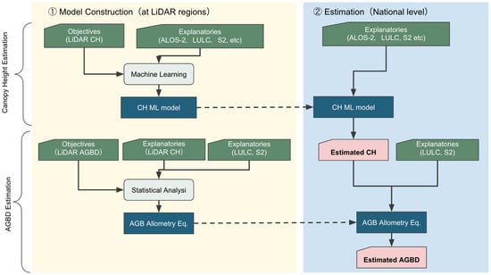
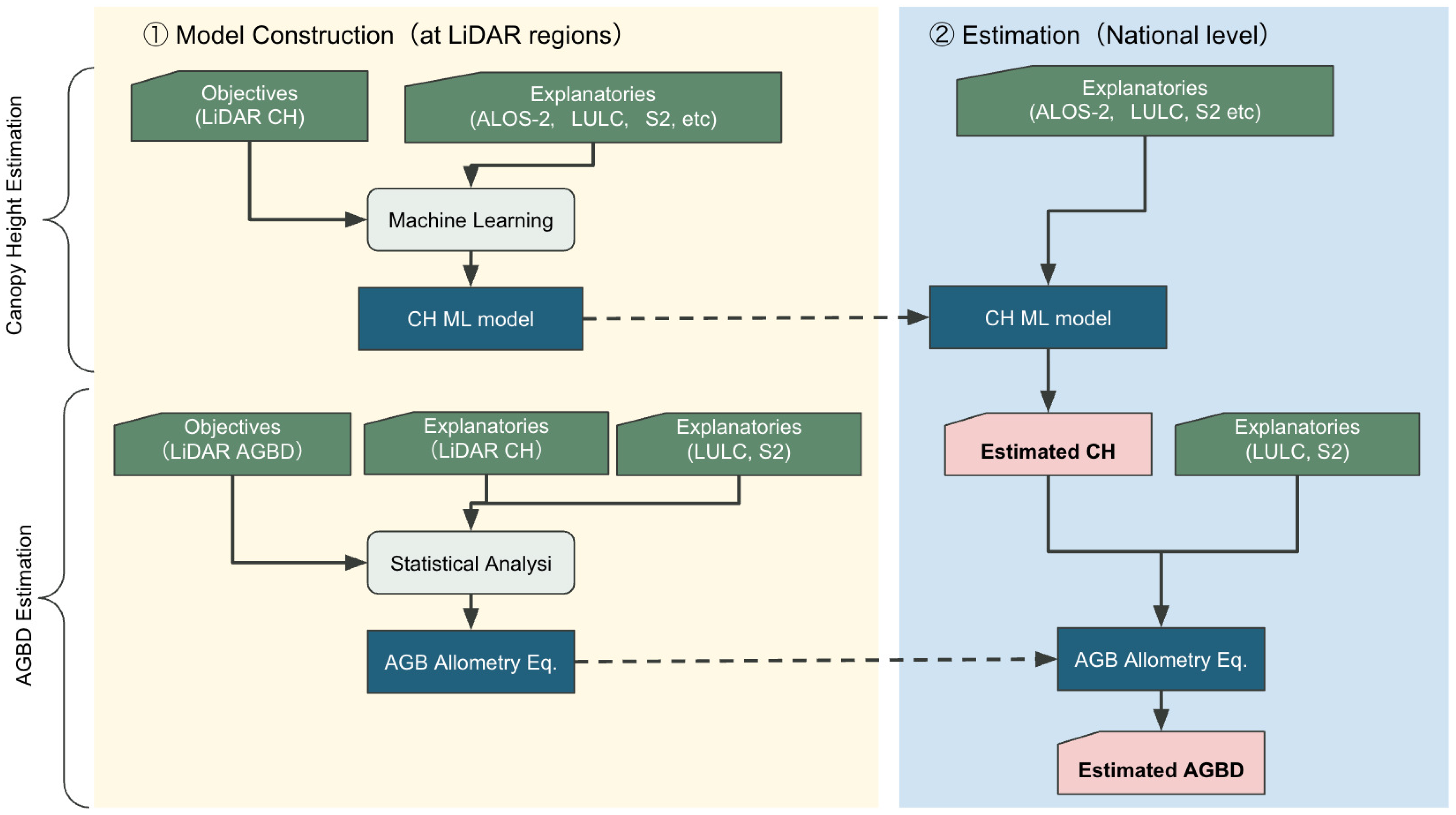
In the development of carbon budget estimation methods, we verified an AGB estimation method using average canopy height estimation and its results. In the development of average canopy height estimation and AGB estimation methods, we created average canopy height and AGB data with a resolution of approximately 10 m using airborne LiDAR data. In addition to the training data, spectral information and various indices from various satellite data, including PALSAR-2, were utilized as learning data to construct a dataset. Based on the constructed dataset, we investigated effective methods for creating forest biomass maps in Japan by conducting data screening, preprocessing, and algorithm selection and evaluation. We developed a logic for estimating the average canopy height of forests correlated with AGB and calculating AGB based on the estimated values, which entire process overview is shown at Figure 1.
Figure 1.
Schematic diagram of processing flow via modeling and estimation.
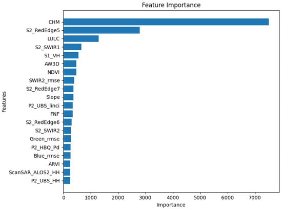
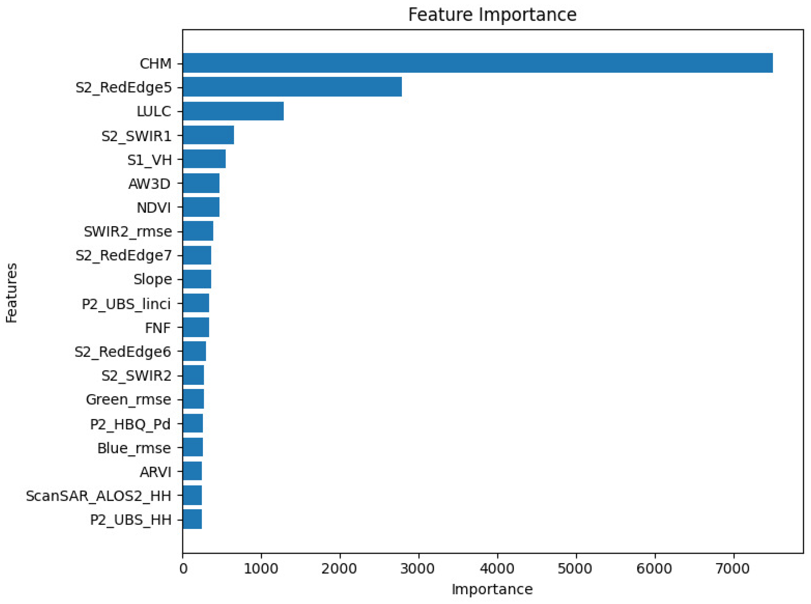
For the estimation of average canopy height, we adopted a decision tree-based XGBoost model and confirmed that the canopy height model (CHM) calculated from digital surface model (DSM) of the ALOS World 3D (AW3D) and digital terrain model (DTM), Sentinel-2 RedEdge5 and SWIR1 and the LULC category variable were effective features for estimation based on the results of feature importance evaluation. For AGB calculation, we created an allometric equation based on the relationship between average canopy height obtained from airborne LiDAR and AGB. Furthermore, by adjusting the parameters of the allometric equation for each forest type (evergreen coniferous, evergreen broadleaf, deciduous coniferous, and deciduous broadleaf), we selected an appropriate calculation equation for each forest type. Using the above average canopy height and AGB calculation logic, a national forest biomass map was created. During the estimation of average canopy height, there were areas where satellite data necessary for inference was missing, so missing values were interpolated using spatial interpolation methods. The accuracy of the existing biomass map and developed AGB map were compared by cross-referencing them with ground measurements taken at multiple locations within the country. The results confirmed that the developed AGB map showed the highest correlation.
For evaluations, we employ the Root Mean Square Error (RMSE), coefficient of determination (), Mean Absolute Percentage Error (MAPE) and ratio of estimates within ±20% of the ground truth as measures of accuracy. RMSE, and MAPE are formulated as
where is the ground truth, is the prediction, and is the mean of the ground truth.
3.1. Pre-Pocessing
LiDAR data preparation in Table 3 shows the location and year of the data used. To incorporate Japan’s diverse environmental conditions into the model, the training dataset was constructed by selecting representative areas from three distinct regions: the Sea of Japan side, the Pacific side, and the Inland region. The Sea of Japan side is characterized by heavy winter snowfall, which has a unique influence on forest stand structure and tree morphology. In contrast, the Pacific side features high precipitation during summer driven by the southeast monsoon, while winters are generally dry with frequent clear weather, providing favorable light conditions for temperate forest growth. The Inland region, surrounded by mountains, experiences relatively low annual precipitation and large seasonal temperature fluctuations, resulting in forest dynamics that differ from those of coastal areas. By encompassing these regions, the model integrates forest data reflecting the diverse environmental patterns found across Japan. We checked the attribute information and used canopy height and biomass as teacher data. We identified tree tops within each 1/12,000-degree pixel, calculated statistics, and rasterized them. Canopy height was calculated as the average within the pixel, and AGB was calculated as the total sum. Finally, the total biomass given was divided by the area of this pixel in hectares to obtain the biomass density per hectare.
Table 3.
LiDAR data used in the dataset.
To minimize the effects of snow and leaves, Sentinel-2 L2A (atmosphere-corrected reflectance) and cloud probability data were acquired, and only pixels with a cloud probability of 30% or less were used. To avoid summer, when NDVI and NIR values are overestimated due to leaf effects, the median values of the target bands were calculated from spring (April to June) and autumn (September to October) data. To obtain long-term change characteristics, Landsat 8 L2 data (2014–2024) was used and masked using the CLOUD_COVER_LAND < 50% and QA_PIXEL bands, and the RMSE of the selected bands was calculated using CCDC. To mitigate the effects of seasonal variations and complement SAR data, the DN values from PALSAR-2 ScanSAR Level 2.2 were converted to (Equation (4)), and the median values from June to October were obtained.
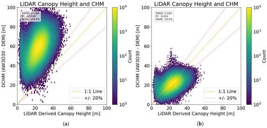
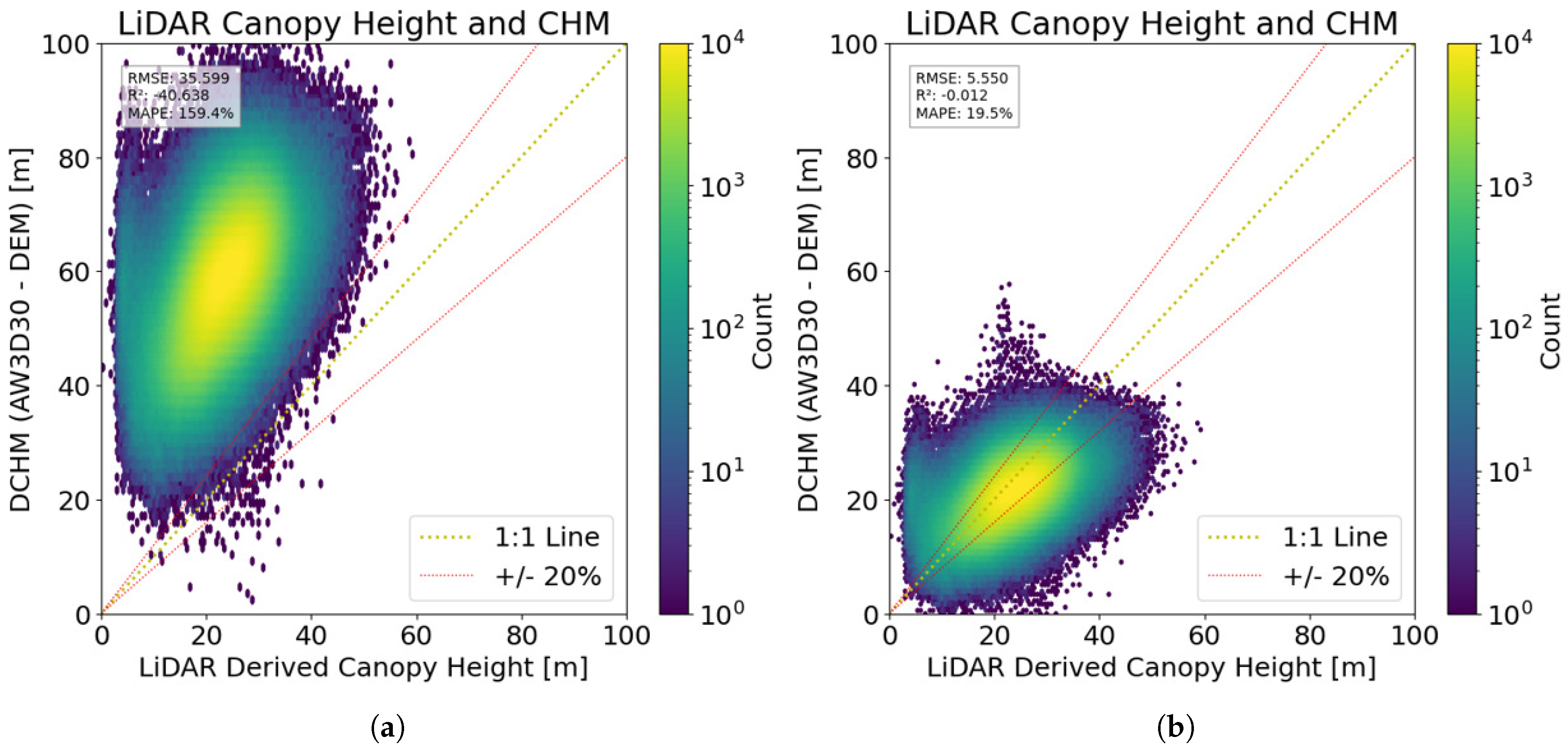
When considering valid explanatory variables, we initially planned to use the simple difference between AW3D and DEM as a feature, but a discrepancy was found between this and the average canopy height calculated using LiDAR. Therefore, we adjusted the coefficients to increase the correlation with the LiDAR canopy height and finally calculated the canopy height model (CHM) using a calculation formula and adopted it as an explanatory variable. Following this adjustment, although some variance remained, the RMSE improved significantly from 35.599 m to 5.550 m, and the MAPE was reduced to 19.5% (Figure 2, right). Consequently, we adopted this calibrated CHM as a primary explanatory variable for our model. The coefficients were determined through a linear fitting process to ensure consistency between the estimated features and the heights derived from LiDAR.
To improve the quality of the learning data and ensure the accuracy of the analysis, we cleaned the dataset, including satellite data and LiDAR data, according to the procedure in Table 4. In this process, pixels located at forest boundaries were excluded, as forest edges often contain mixed pixels of forest and non-forest that reduce the reliability of reference values. A ScanSAR threshold of 0 was set to remove physically invalid scattering noise. Furthermore, a lower limit of 10 Mg/ha was applied to the AGBD to exclude pixels where the land was classified as forest in the LULC map but actually contained little to no vegetation; including such near-zero values would have introduced a downward bias in the model’s training. The upper limit of AGBD (1000 Mg/ha) was determined because the distribution of AGB derived from airborne LiDAR in Japan shows that values exceeding this threshold are statistical outliers. The elevation threshold, defined by the 3 standard (1045 m), corresponds to the maximum elevation in the training dataset and was applied to prevent uncertain extrapolations.
Table 4.
Dataset preprocessing.
3.2. Canopy Height Estimation
In the training data set for canopy height estimation, the data in Table 1 and the CHM calculated in Equation (5) were used, and as noted above, only data from sites with elevations below 1045 m were selected for training. For DEM, we avoided employing it as an explanatory variable because of the limited elevation data provided. For machine learning, the XGBoost model was used for the purpose of canopy height estimation, and an objective function featuring variance weighting based on kernel density estimation (Gaussian KDE) was incorporated for training. The objective function L is expressed by the following equation:
where is the predicted value, is the true value, is a small constant epsilon to prevent zero division, and is the kernel density estimate (Gaussian KDE) for . The objective function is a standard MSE loss function that calculates the squared error between the predicted value and the true value multiplied by a weight based on the kernel density of the target (KDE); the smaller the KDE (the less frequently occurring value), the greater the loss, allowing the model to be trained to account for bias in the data distribution. This enables the learning of models that take into account the bias of the data distribution. As shown in Equation (6), this is a means to address bias in the training data set.
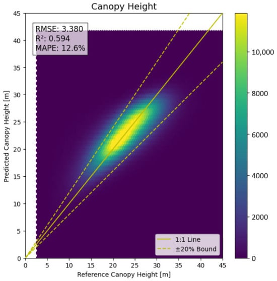
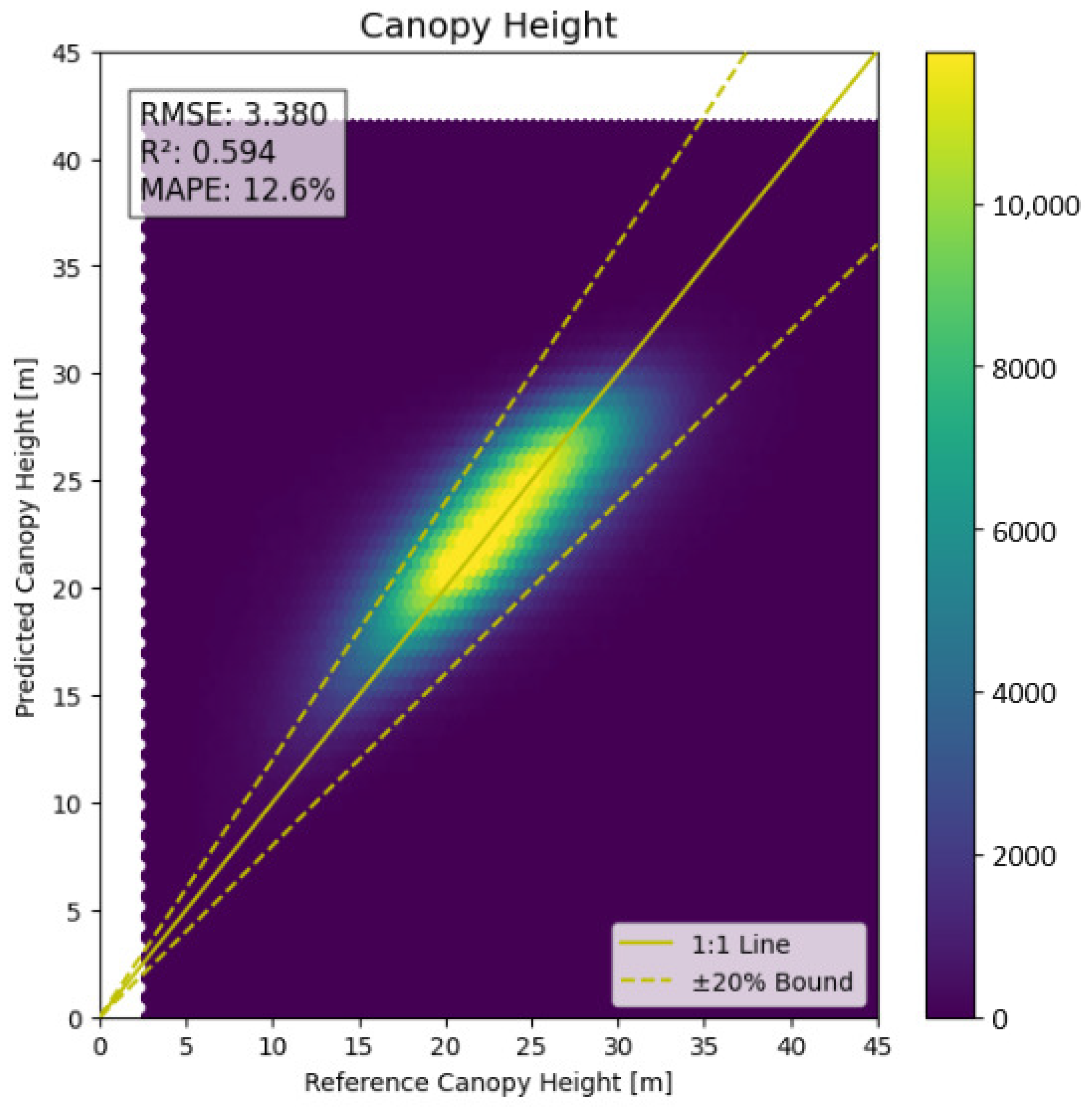
The hyperparameters of the model were evaluated and optimized using Random Search (RSE), with combinations randomly chosen within the ranges shown in Table 5. The results of tree height estimation using the above learning parameters are shown in Figure 3. The feature importance for the canopy height estimation model (Figure 4) reveals distinct variations in the contributions of different input variables.
Table 5.
Hyperparamter options for tuning.
Figure 3.
Learning result for canopy height.
Figure 4.
The feature importance in machine learning for the canopy height.
3.3. Allometry Formulation for AGBD
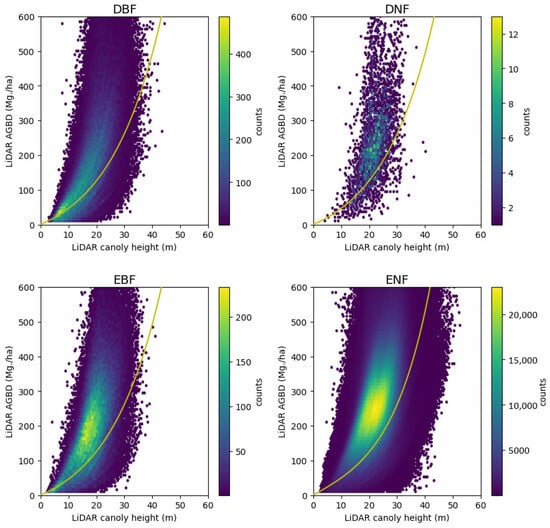
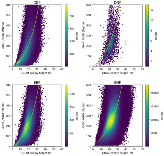
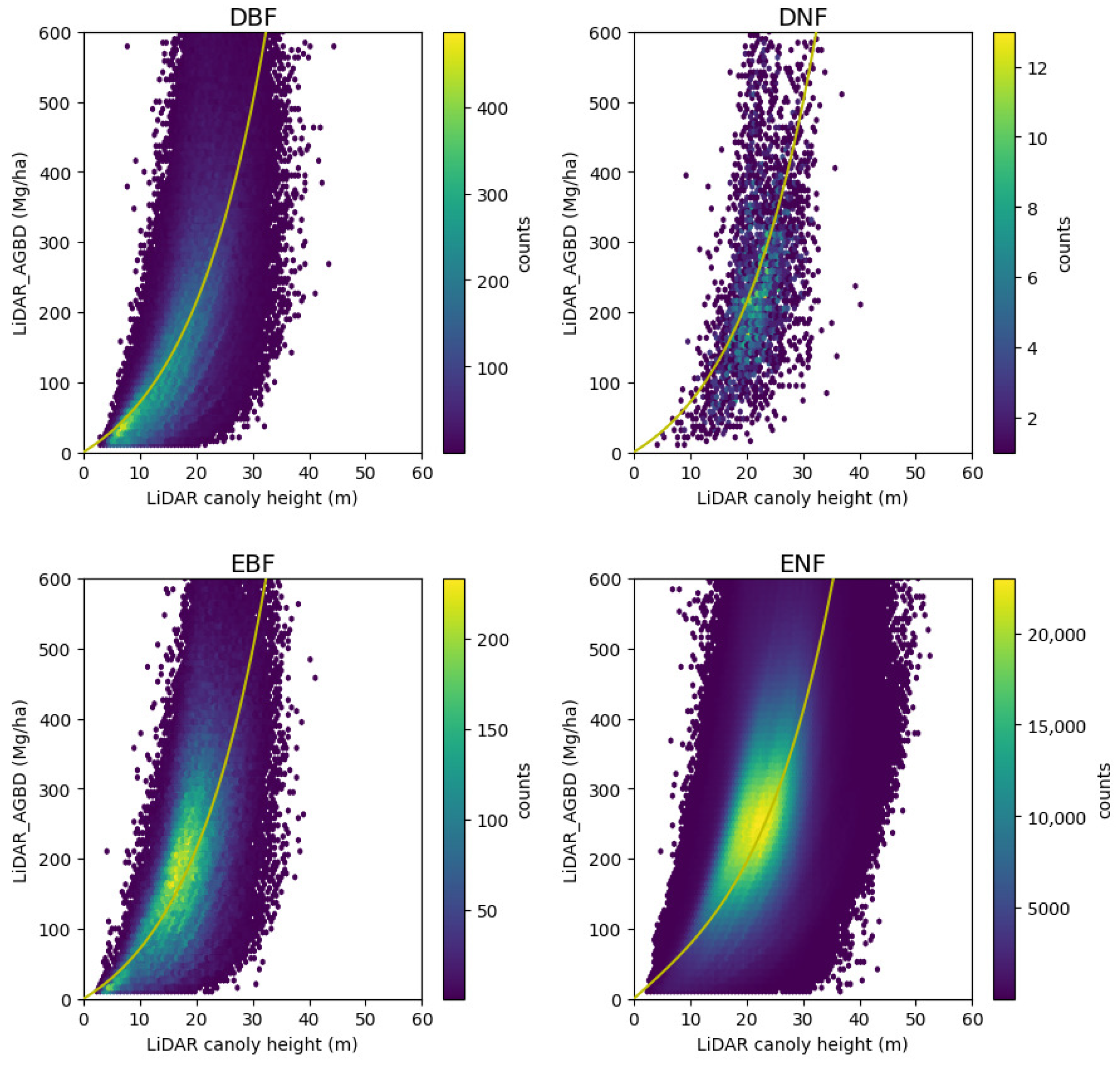
This study develops allometry equations for each tree type to calculate biomass density from average canopy height. Unlike allometry equations in general, which are for a single tree, our allometry equations are for the area-based density of AGB. When directly estimating AGB values, the uneven distribution of training data caused the model to predict intermediate AGB values, especially in areas with limited samples such as low-AGB and high-AGB regions. This reduced the generalizability of the model across Japan’s diverse forest types. To address this issue, we adopted an allometry-based approach, which leverages the strong correlation between canopy height and AGB. To suppress systematic overestimation caused by outliers, an upper limit of 600 Mg/ha was set based on statistical information from the nationwide dataset. This mitigates overestimation resulting from measurement noise or extreme anomalies, thereby improving the overall reliability of the model. By utilizing pixels with LiDAR-measured canopy height and AGBD as the ground truth, an exploratory analysis suggests the exponential relationship between the average canopy height and the biomass density for four tree types; DBF, DNF, EBF and ENF. For bamboo forest, we set a constant value, as described at the end of this section. As a result of exploratory analysis, the following two equations are selected as candidates for the allometry equation because they have exponential properties and pass through the origin.
These functions are optimized with the L2 norm (by scipy.optimize.least_squares). The parameters, optimality (score), and adoption choices for each tree type are summarized in Table 6. The adopted allometry equations are plotted in Figure 5 with CH and AGBD from LiDAR measurements.
Table 6.
Optimized parameters and adoption of the allometry equation for each tree type.
Figure 5.
LiDAR AGBD against LiDAR canopy height with allometry function optimized with L2 norm for each tree type.
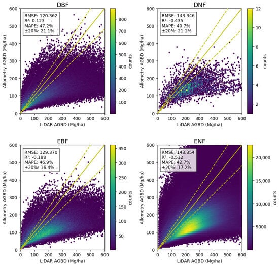
As Figure 5 and Figure 6 show, most cases are underestimated. Hence an additional adjustment is made to the term A. With the ratio of the ith estimated value of tree type s to the corresponding ground truth ,
the adjusted estimation is derived as
where is the average of the first and the third quartiles of for the tree type s. The allometry equations after this ratio adjustment are
Figure 6.
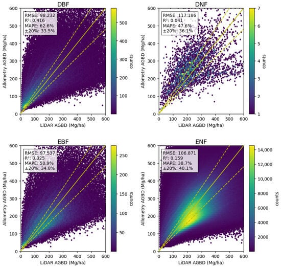
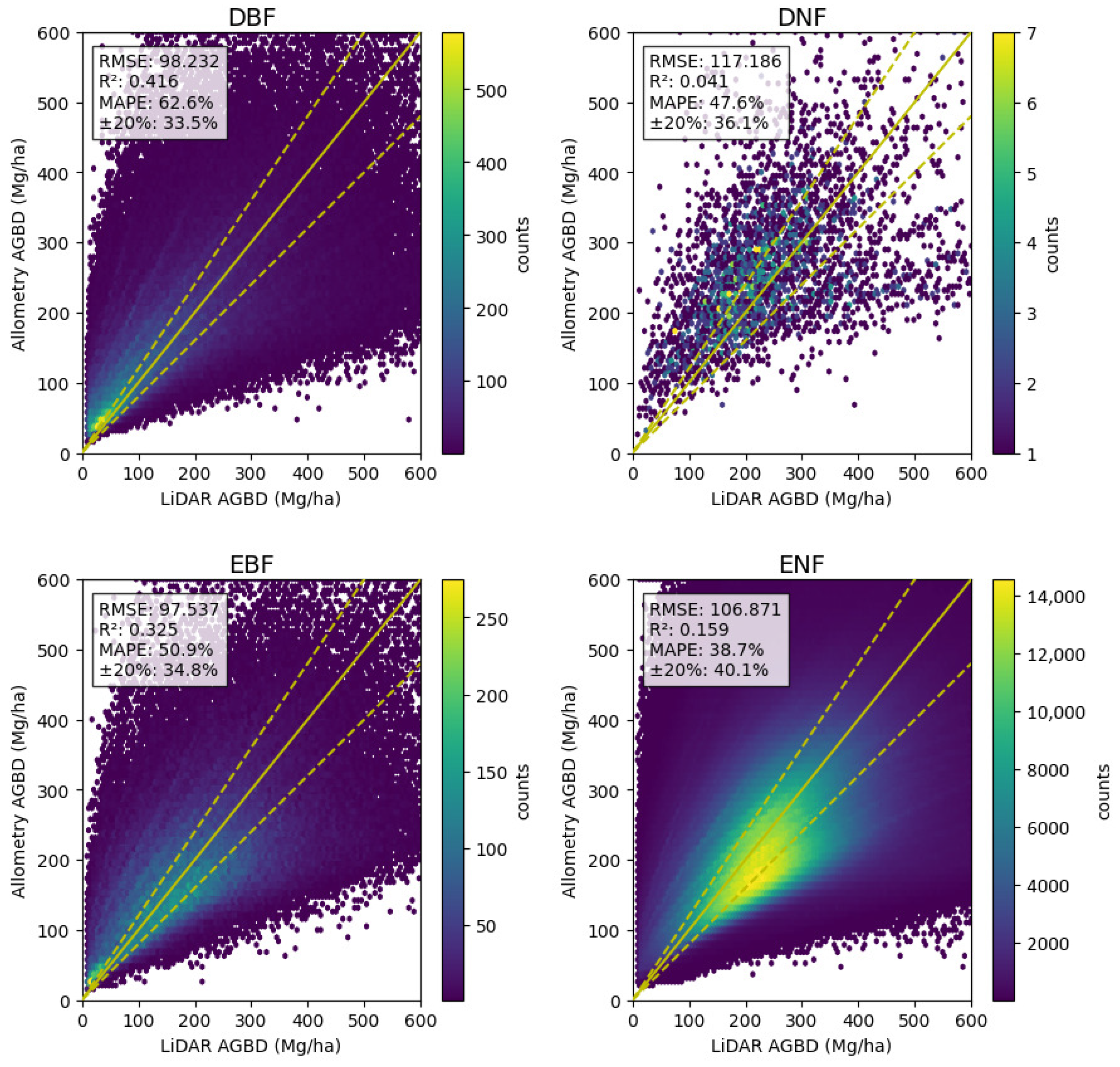
Hexbin plots of estimated AGBD after L2 optimization against LiDAR AGBD used for the optimization are shown for each tree type. The yellow solid line indicates a 1–to–1 relationship with LiDAR measurements. Two yellow dashed lines indicate a ±20% range from the LiDAR measurements. Measures of accuracy (RMSE, , MAPE, and ratio of estimates within 20% of the ground truth) are shown in the box at the top left.
These allometry equations are plotted with LiDAR CH and AGBD in Figure 7.
Figure 7.
Similar to Figure 5 with allometry functions optimized with L2 norm and adjusted with the ratios.
Because objective data is selected as that for which AGBD is less than or equal to 600 Mg/ha, adjustment of the allometry equations is finalized with an upper limit of 600 Mg/ha over the estimated AGBD in Equations (11)–(14).
The final results are shown in Figure 8. We briefly note here that scores (i.e., ) have been slightly improved with this upper limit. Airborne LiDAR mainly targets forest areas and does not focus on grasslands and bamboo forests. Hence bamboo forests are not included in the training data. However we do not want bamboo forests blank on our AGB map. Therefore we utilize the average ABGD value of managed bamboo forests (34.4 Mg/ha) and that of unmanaged bamboo forests (66.3 Mg/ha) of the most common species of bamboo in Japan [23] and adopt their average value of 50.53 Mg/ha for this study.
Figure 8.
Our estimated AGBD with the upper limit of 600 Mg/ha against LiDAR AGBD used for optimization is plotted for each tree type in a similar manner to Figure 6.
4. Results
4.1. National-Level Tendencies
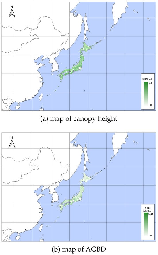
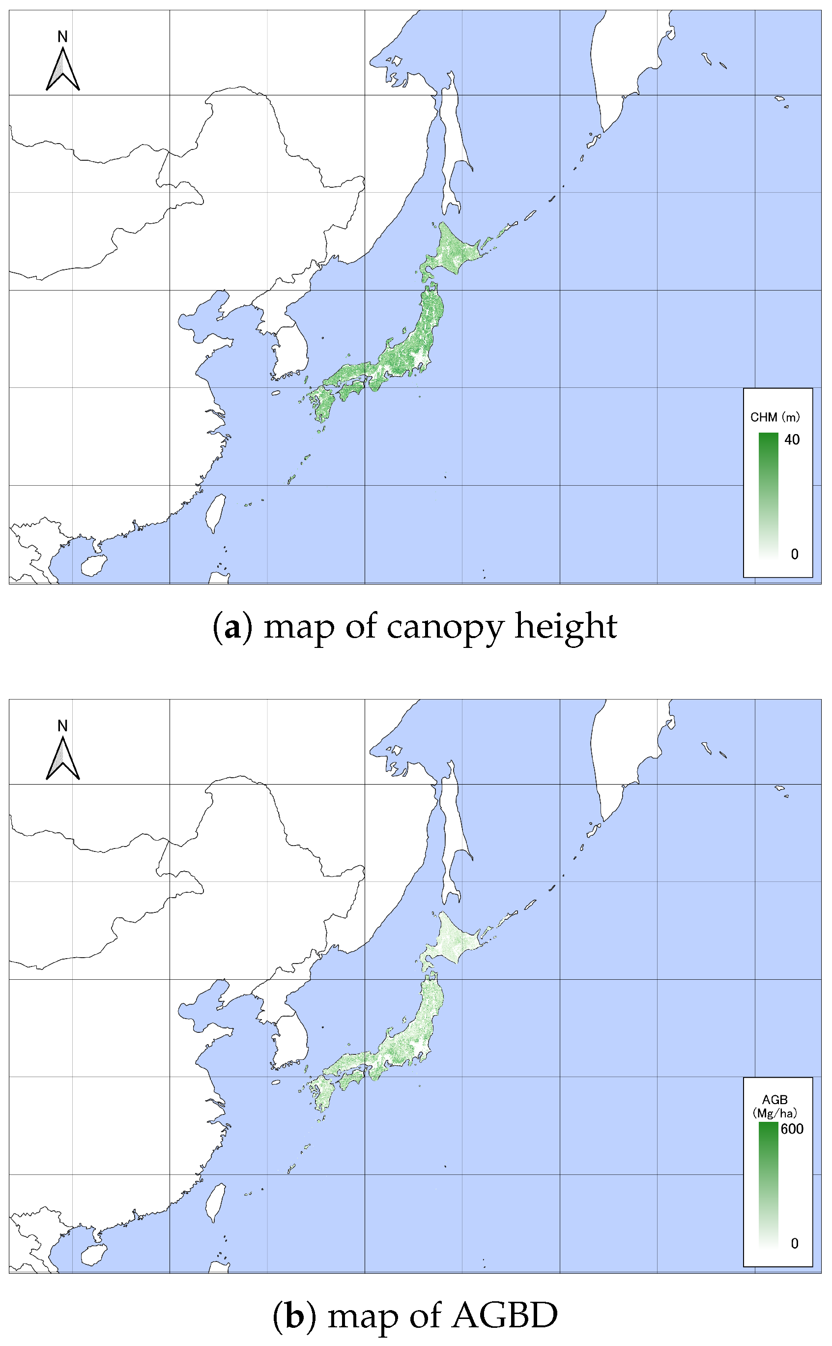
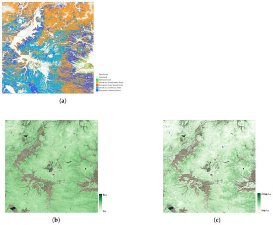
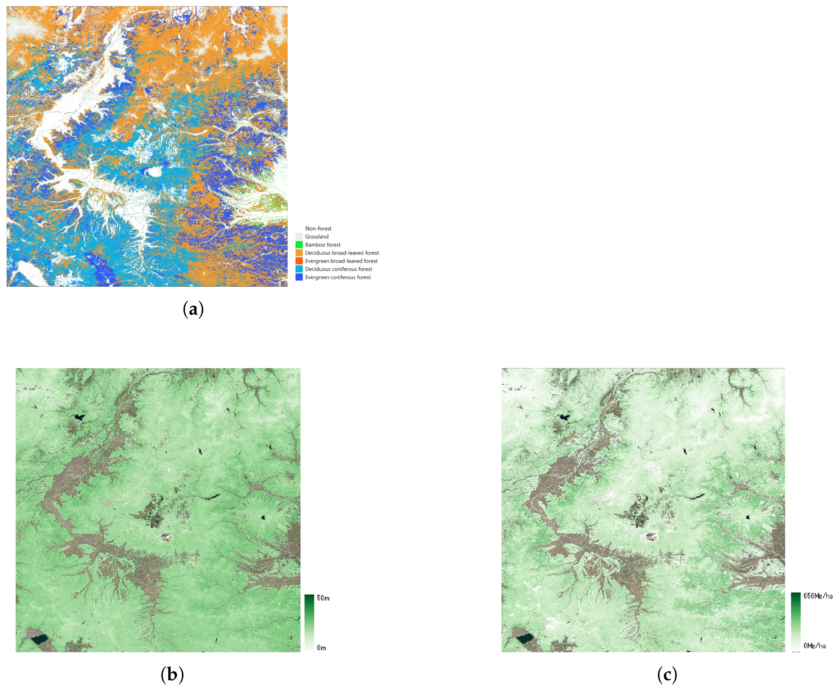
Our national maps of canopy height and AGBD are shown in Figure 9. To provide a more detailed assessment of the spatial distribution, Figure 10 presents a regional zoom of the study area, incorporating land cover classification (Figure 10a) alongside canopy height (Figure 10b) and AGBD (Figure 10c). Japan consists of 47 prefectures, which are categorized into seven jurisdictions. The detailed breakdown of each jurisdiction and its constituent prefectures is presented in Table 7. After generating the national maps, the distribution densities of the estimated canopy height (CH) and above-ground biomass density (AGBD) are presented for each jurisdiction.
Figure 9.
National-level overview of (a) canopy height and (b) AGBD.
Figure 10.
Regional zoom of (a) land cover classification, (b) canopy height, (c) AGBD.
Table 7.
Jurisdiction and prefectures in Japan.
4.2. Validation with LiDAR Data
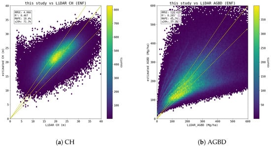
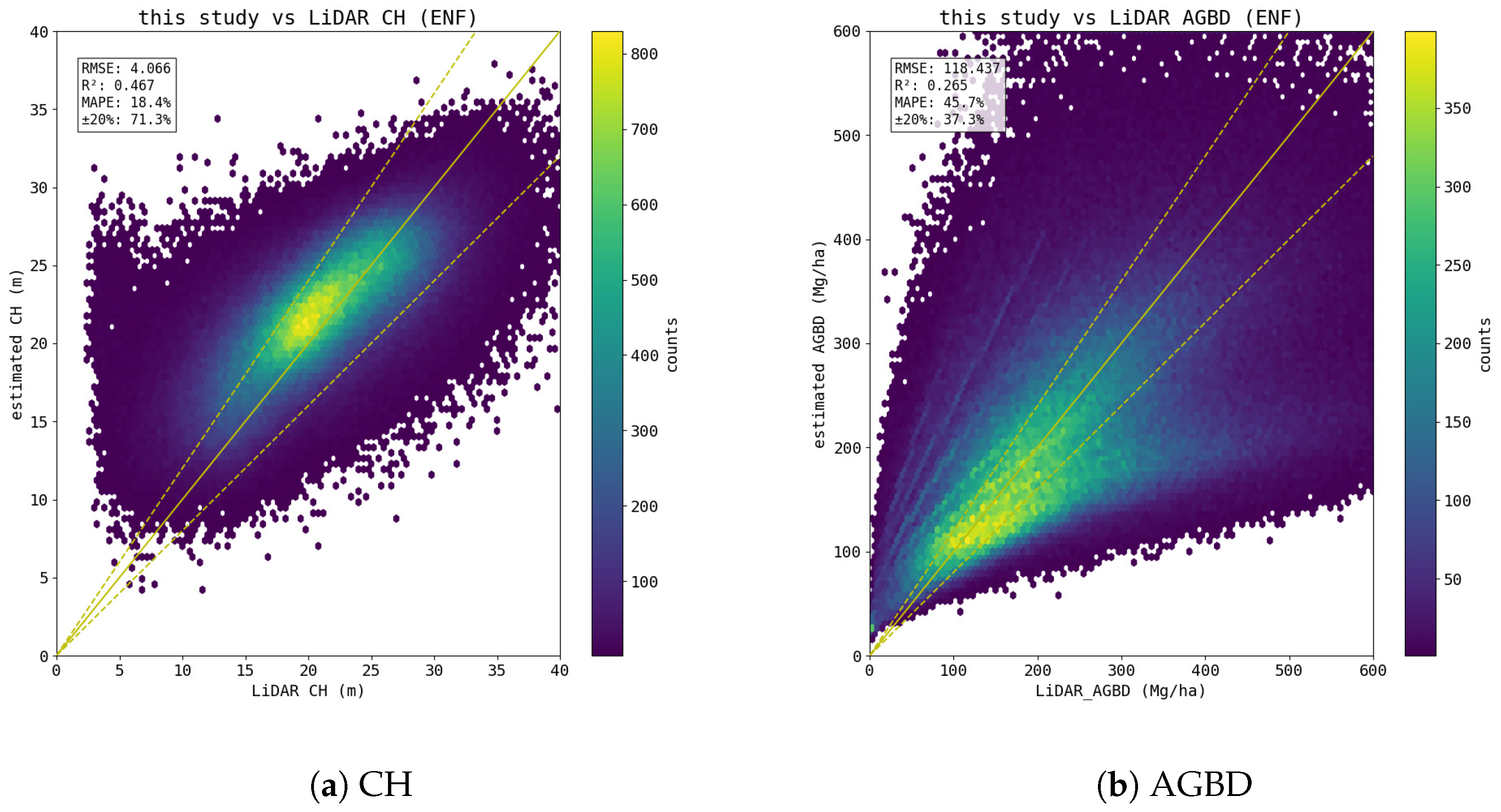
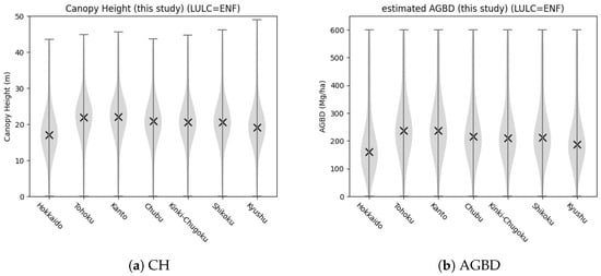
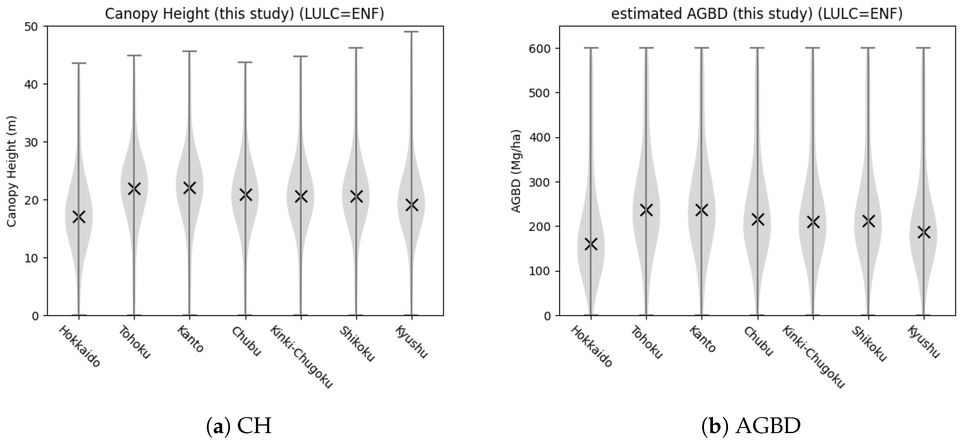
Using three 2nd-mesh data points, which are excluded from the training data, estimates of canopy heights and AGBD are compared with LiDAR measurements. To validate the model’s performance, we selected evaluation meshes from distinct geographical divisions—the Sea of Japan side, the Pacific side, and the Inland region. This selection accounts for variations in precipitation and snowfall patterns, which significantly influence forest structures across Japan. Figure 11a shows that the core part (yellow part) stretches along the one-to-one line (yellow solid line) with a slight tendency for overestimation. Measures of accuracy for canopy height estimates are RMSE of 4.066 m, of 0.467, and MAPE of 18.4%, and 71.3% of estimates fell within ±20% of LiDAR measurements. For AGB, estimates are distributed widely beyond the lines of ±20% (yellow dashed lines) but show no saturation for higher values of AGBD. Measures of accuracy are RMSE of 118.437 Mg/ha, of 0.265, and MAPE of 45.7%, and 37.3% of estimates fell within ±20% of LiDAR measurements. Figure 12 shows regional variations in estimated (a) canopy height (CH) and (b) aboveground biomass density (AGBD) for evergreen needleleaf forests across seven jurisdictions. Both parameters share similar geographical trends. Hokkaido exhibited the lowest averages (mean CH: 17 m; mean AGBD: 160 Mg/ha), with distributions skewed toward lower values. Conversely, Tohoku and Kanto showed the highest averages (mean CH: 22 m; mean AGBD: 240 Mg/ha); their broader violin shapes at higher intervals indicate a larger proportion of mature, high-biomass forests. From Chubu southward to Kyushu, mean values decreased gradually but remained stable (CH: 19–21 m; AGBD: 190–220 Mg/ha). Although Kyushu had slightly lower averages, its distribution extended to a maximum CH near 50 m, reflecting localized, exceptionally tall stands.
Figure 11.
Validations of (a) estimated canopy height and (b) AGBD are made against LiDAR measurements not used for learning and optimization. Plots are drawn in a similar manner to Figure 6.
Figure 12.
Violin plots of our estimates of (a) CH and (b) AGBD. Crosses denote corresponding averages for every jurisdiction.
5. Discussion
In this section, we compare our biomass map with two other published biomass maps, one being the biomass map by the CCI [7]. CCI is a GEDI-based global biomass map.
5.1. Other Published Biomass Maps by Jurisdiction
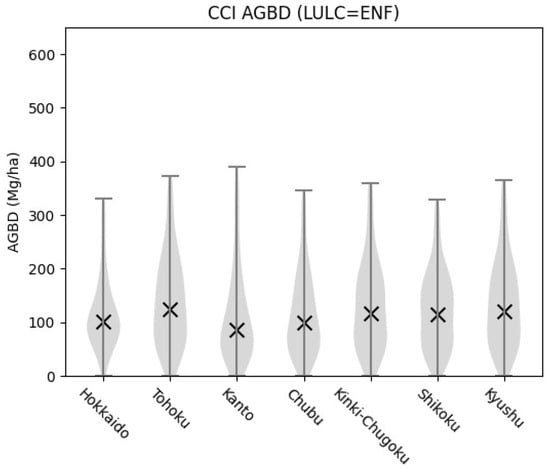
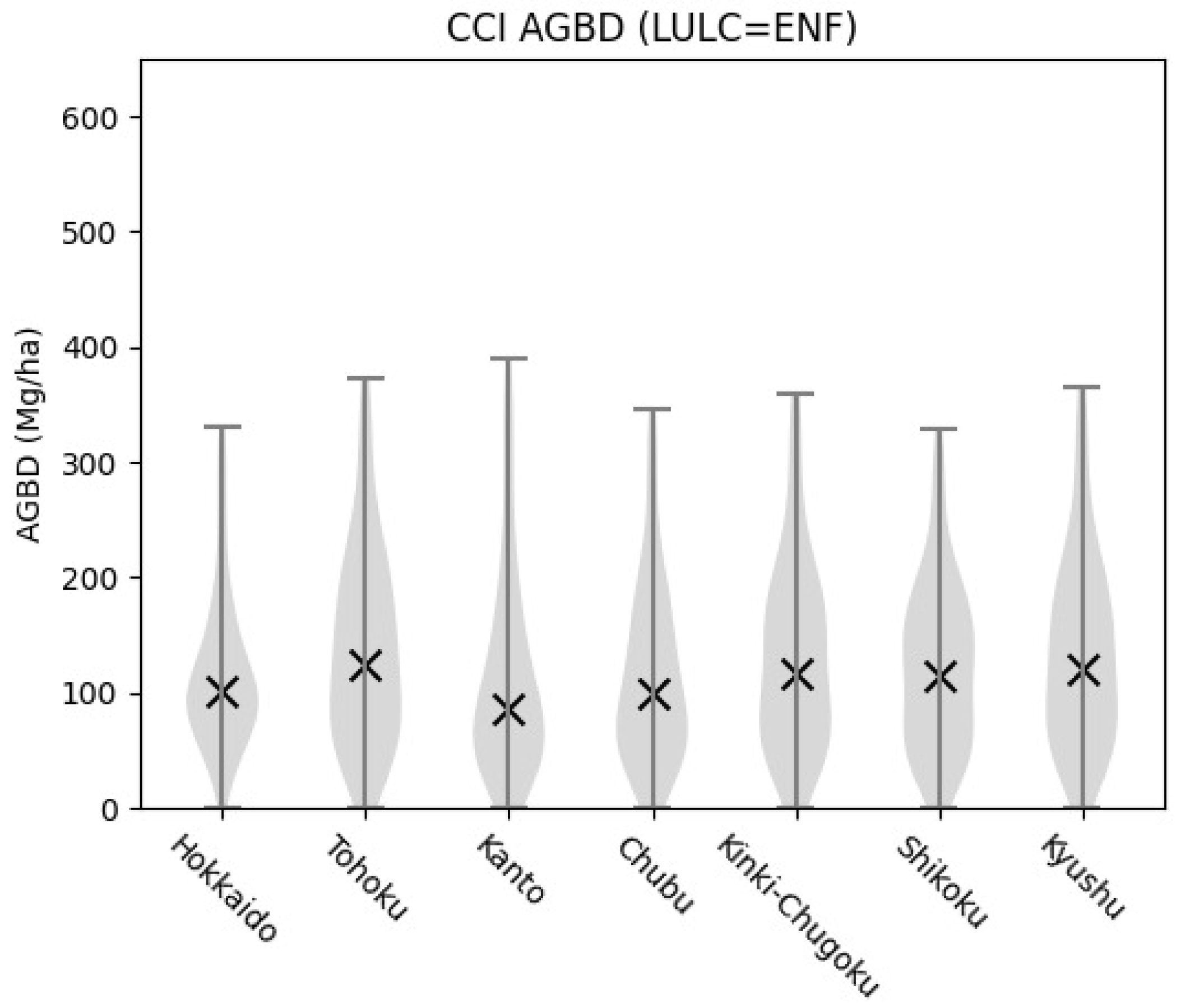
This study organized the CCI AGBD data by jurisdiction, and the results indicate that the distribution of biomass from Hokkaido in the north to Kyushu in the south shows broadly similar patterns across regions. As shown in Figure 13, the CCI product tends to report relatively lower AGBD values, with mean estimates around 100 Mg/ha for each jurisdiction. Median biomass densities generally fall within 100–150 Mg/ha, and large regional differences are not evident. In practice, however, forests in Japan exhibit considerable ecological variation: for example, cold-temperate coniferous forests in northern regions such as Hokkaido and Tohoku are structurally and dynamically different from warm-temperate broadleaf forests in Kyushu and Shikoku. Moreover, field observations confirm that some forest stands reach up to 600 Mg/ha, whereas the CCI product is generally limited to 300–400 Mg/ha. These findings suggest that while the CCI dataset is valuable for global-scale consistency, it may not fully capture the high-biomass stands and region-specific forest characteristics present in Japan. This potential underestimation could stem from the emphasis on global applicability rather than local ecological diversity.
Figure 13.
Violin plots of AGBD estimated by CCI for each jurisdiction in similar manner to Figure 12.
5.2. Comparison of Biomass Maps with LiDAR
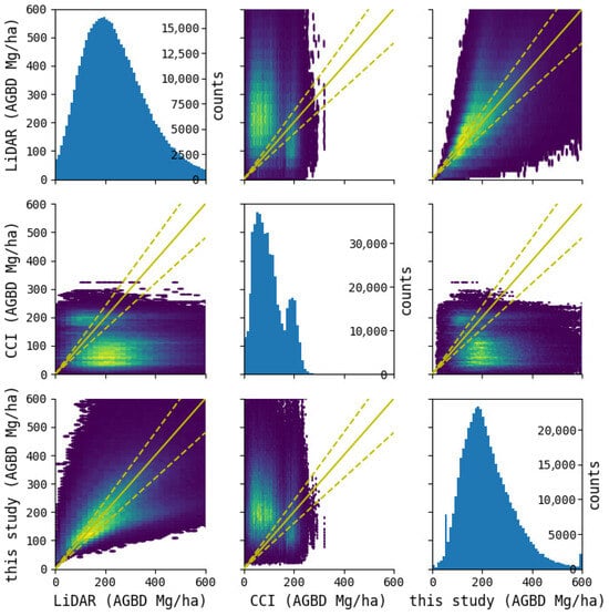
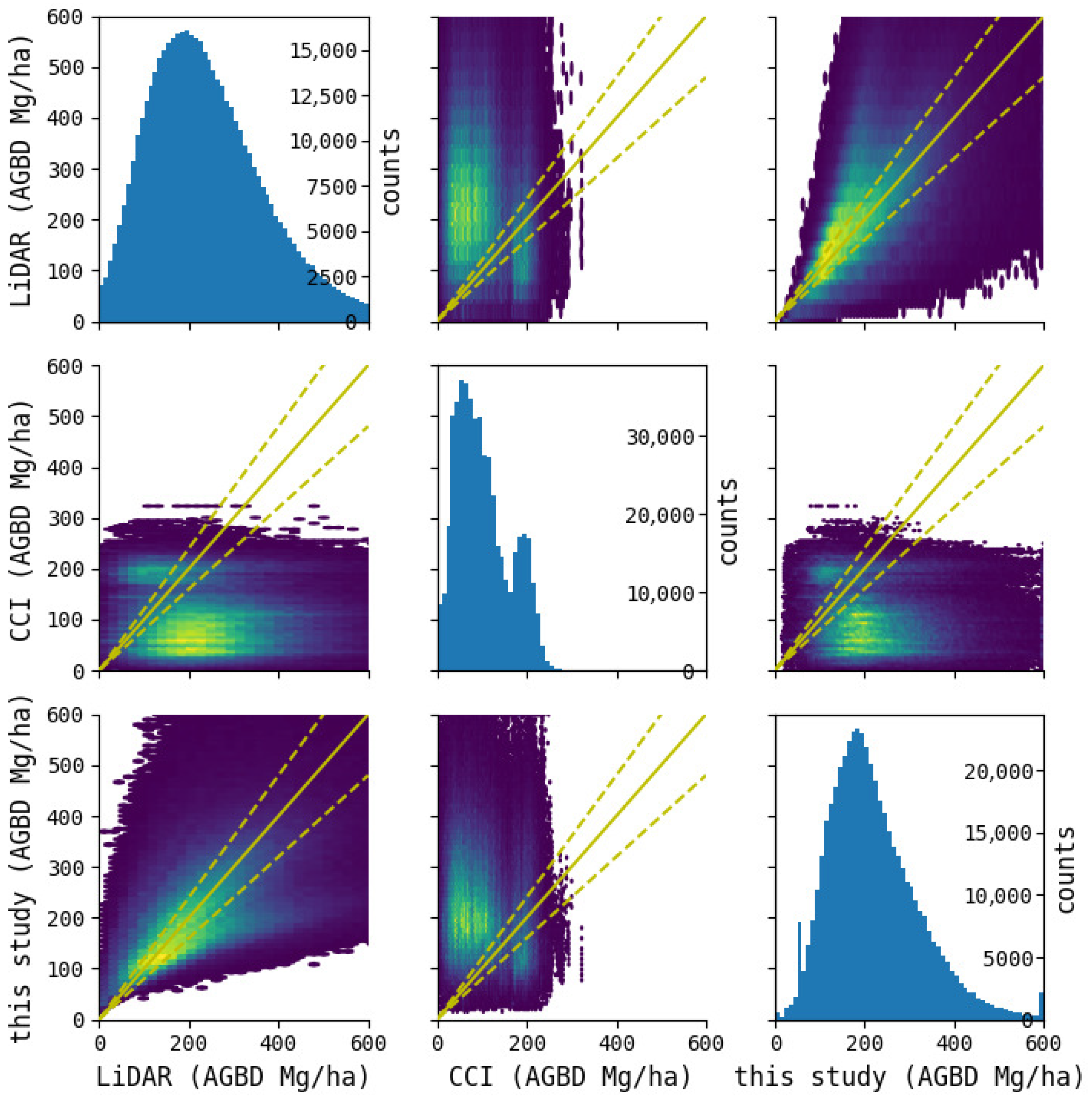
As we have seen, our AGBD estimates appear to have a more reasonable relationship with actual measurements than the CCI biomass map. Table 8 summarizes the accuracy metrics for AGBD relative to LiDAR measurements across the validation data. This table clearly shows that our biomass map achieves superior scores across all accuracy metrics. Figure 14 displays the AGBD distribution for pixels with available LiDAR measurements across the validation data. It is evident that the distribution of our biomass map more closely resembles the distribution of LiDAR measurements than the other biomass maps.
Table 8.
Comparison of biomass maps with measures of accuracy for AGBD at validated 2nd-mesh tiles.
Figure 14.
Pairplot of aboveground biomass density (AGBD) estimates from LiDAR, CCI, and this study.
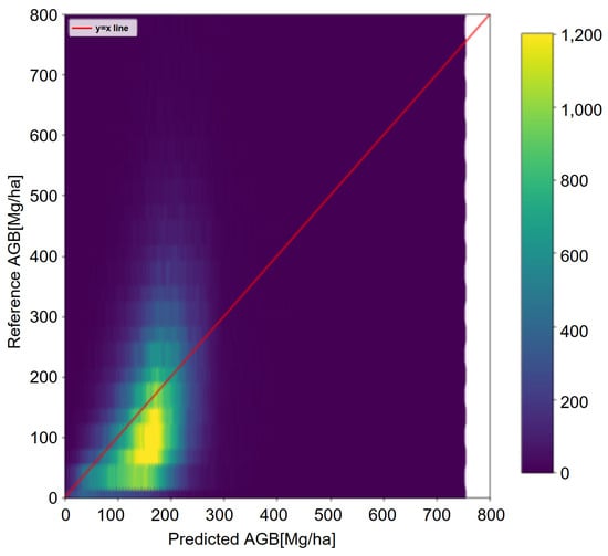
The key difference between this model and the other two models lies in the adoption of optimization techniques using allometric equations rather than machine learning technology. This addresses the limitation of existing machine learning, which struggle to perform well in high-biomass regions due to biased learning data distributions caused by insufficient samples in those regions. The allometric equations introduce physical consistency constraints that compensate for this bias. Consequently, this model suppresses underestimation even in high-biomass regions and demonstrates superior accuracy across all indicators. To verify the effectiveness of the allometric equations, we conducted an ablation experiment in which AGBD was directly estimated using XGBoost. As shown in Figure 15, the direct estimation results saturated at approximately 200 Mg/ha, a trend consistent with existing maps such as CCI. These results demonstrate that the proposed method, which couples height estimation with allometry, effectively mitigates the saturation problem inherent in traditional direct biomass regression.
Figure 15.
An example of saturated AGBD estimation by XGBoost without allometric constraints.
However, several limitations remain. For example, forest types such as bamboo stands and DNF may exhibit reduced estimation accuracy due to structural heterogeneity and the limited availability of representative training data. Addressing these issues may require incorporating high-resolution airborne LiDAR, long-term field plots, and refined allometric equations tailored to specific forest types. Tackling these challenges will be essential for further enhancing the reliability of nationwide biomass maps. Also, since actual biomass is strongly influenced by stand density and canopy density, incorporating these structural variables into the estimation model will be a critical next step for future research.
5.3. Uncertainties and Future Directions in the Two-Stage Model
The two-stage modeling framework adopted in this study—first estimating canopy height and then deriving AGB using allometric equations—is a highly effective approach for AGB estimation. In particular, a major advantage of this model is its ability to avoid signal saturation in high-biomass regions, which has been a long-standing challenge in conventional remote sensing methods. However, this approach involves a trade-off regarding error propagation. Because non-linear allometric equations (typically power functions) are used in the second stage for AGB calculation, there is a risk that minor deviations or noise originating from the input data is amplified by this non-linearity, manifesting as larger absolute errors in the final estimates. The primary source of this error stems from the uncertainties of the input data in the first stage. Our feature importance analysis revealed that topographic variables, specifically DEM and AW3D, made extremely high contributions to the model’s predictions. This implies that, in addition to common sensor-specific noise—such as remnant clouds and shadows in Sentinel-2 or topographic effects and saturation in PALSAR-2—localized discrepancies and errors in DEM/DSM data directly lead to uncertainties in the initial canopy height estimation.
Therefore, to reduce these propagated errors and improve estimation accuracy in future studies, it is essential to enhance the precision of the input data, particularly the topographic data that highly contribute to the model. The availability of such high-precision topographic data, however, varies geographically. While certain regions, such as Japan, benefit from detailed national datasets (e.g., the 0.5 m resolution elevation data provided by the Geospatial Information Authority of Japan), many areas globally rely on widely available remote sensing-based elevation products. These global products may lack sufficient resolution or contain inherent errors. Consequently, when applying this method to other regions to perform equivalent canopy height and AGB estimations, the precise development and preparation of foundational DEM data will be a critical future challenge.
6. Conclusions
In this study, we estimated canopy height at the national scale of Japan using a machine learning model that combined optical and SAR satellite data with aircraft LiDAR data and constructed a 10 m resolution map of above-ground biomass density (AGBD) across Japan (Biomass Map) using allometry equations optimized for each forest type. The validation results showed improved estimation accuracy, particularly in high-biomass areas, compared with existing maps, demonstrating that this method can effectively capture diverse forest types, including broadleaf forests. These outcomes are expected to contribute to nationwide forest carbon stock assessments and future forest change monitoring.
To further improve the accuracy of biomass estimation in Japan, it is expected that incorporating airborne LiDAR data from a wider range of locations will enhance the representativeness of the training data. In particular, as the current training dataset has a limited representation of cold-climate regions, incorporating data from these areas will be essential to better reflect regional forest characteristics. In addition, because tree crowns often extend across multiple pixels, creating training data that accounts for crown shape and density is expected to reduce underestimation. By utilizing temporal features from satellite data, such as PALSAR-2, biomass estimation can also incorporate forest dynamics over time. When selecting satellite data, using observations aligned with the target period enables more consistent long-term monitoring.
For overseas applications, while the future use of P-band SAR is promising, canopy height-based methods already enable estimation in high-biomass regions. For global-scale application, it will be important to verify biomass estimation methods using satellite data capable of capturing three-dimensional forest structures, such as GEDI.
Author Contributions
A.D.K.: writing—original draft, investigation, conceptualization, data curation, formal analysis, and methodology; T.K.: writing—original draft, writing—review and editing, methodology, conceptualization; T.T.: writing—review and editing, conceptualization, and supervision. All authors have read and agreed to the published version of the manuscript.
Funding
This study was conducted as part of a research project titled “Establishment and Strategic Implementation of Forest Biomass Estimation Methods for Achieving Carbon Neutrality”, the “Strategic Program for Accelerating the Research, Development, and Utilization of Space Technology” (Stardust Program) by the Ministry of Education, Culture, Sports, Science and Technology (MEXT), Japan.
Data Availability Statement
The publicly available datasets analyzed in this study are described in the Section 3. Additional data generated or analyzed during this study are available from the corresponding author upon reasonable request, subject to data-sharing restrictions and permissions from the data providers.
Conflicts of Interest
Authors A.D.K. and T.K. are employed by Archeda, Inc. This study was conducted as part of a commissioned research project with the Japan Aerospace Exploration Agency (JAXA). The remaining author declares that the research was conducted in the absence of any commercial or financial relationships that could be construed as a potential conflict of interest.
References
- Araza, A.; de Bruin, S.; Herold, M.; Quegan, S.; Labriere, N.; Rodriguez-Veiga, P.; Avitabile, V.; Santoro, M.; Mitchard, E.T.; Ryan, C.M.; et al. A comprehensive framework for assessing the accuracy and uncertainty of global above-ground biomass maps. Remote Sens. Environ. 2022, 272, 112917. [Google Scholar] [CrossRef] [Scilit]
- Kanja, K.; Zhang, C.; Atkinson, P.M. Evaluating multi-seasonal SAR and optical imagery for above-ground biomass estimation using the national forest inventory of Zambia. Int. J. Appl. Earth Obs. Geoinf. 2025, 139, 104494. [Google Scholar] [CrossRef] [Scilit]
- Dong, W.; Mitchard, E.T.A.; Chen, Y.; Chen, M.; Cao, C.; Hu, P.; Xu, C.; Hancock, S. Comparing remote sensing-based forest biomass mapping approaches using new forest inventory plots in contrasting forests in northeastern and southwestern China. arXiv 2024, arXiv:2405.15438. [Google Scholar] [CrossRef] [Scilit]
- Duncanson, L.; Kellner, J.R.; Armston, J.; Dubayah, R.; Minor, D.M.; Hancock, S.; Healey, S.P.; Patterson, P.L.; Saarela, S.; Marselis, S.; et al. Aboveground biomass density models for NASA’s Global Ecosystem Dynamics Investigation (GEDI) lidar mission. Remote Sens. Environ. 2022, 270, 112845. [Google Scholar] [CrossRef] [Scilit]
- Yu, J.; Nie, S.; Liu, W.; Sun, Z.; Wang, C.; Xi, X.; Zhu, X.; Fang, M. Evaluating and comparing the performance of ICESat-2 and GEDI data for estimating aboveground biomass in mangroves. Int. J. Digit. Earth 2026, 19, 2627082. [Google Scholar] [CrossRef] [Scilit]
- Santoro, M.; Cartus, O.; Quegan, S.; Kay, H.; Lucas, R.M.; Araza, A.; Herold, M.; Labrière, N.; Chave, J.; Rosenqvist, Å.; et al. Design and performance of the Climate Change Initiative Biomass global retrieval algorithm. Sci. Remote Sens. 2024, 10, 100169. [Google Scholar] [CrossRef] [Scilit]
- Santoro, M.; Cartus, O. ESA Biomass Climate Change Initiative (Biomass_cci): Global Datasets of Forest Above-Ground Biomass for the Years 2010, 2015, 2016, 2017, 2018, 2019, 2020 and 2021, v5.0. NERC EDS Centre for Environmental Data Analysis, 2024. Available online: https://catalogue.ceda.ac.uk/uuid/6666ae0ed0e94bfda0c302f0fe5bec1b (accessed on 10 March 2026).
- Santoro, M.; Cartus, O.; Carvalhais, N.; Rozendaal, D.M.A.; Avitabile, V.; Araza, A.; de Bruin, S.; Herold, M.; Quegan, S.; Rodríguez-Veiga, P.; et al. The global forest above-ground biomass pool for 2010 estimated from high-resolution satellite observations. Earth Syst. Sci. Data 2021, 13, 3927–3950. [Google Scholar] [CrossRef] [Scilit]
- Buchhorn, M.; Lesiv, M.; Tsendbazar, N.E.; Herold, M.; Bertels, L.; Smets, B. Copernicus Global Land Cover Layers—Collection 2. Remote Sens. 2020, 12, 1044. [Google Scholar] [CrossRef] [Scilit]
- Ghosh, S.M.; Behera, M.D. Aboveground biomass estimation using multi-sensor data synergy and machine learning algorithms in a dense tropical forest. Appl. Geogr. 2018, 96, 29–40. [Google Scholar] [CrossRef] [Scilit]
- David, R.M.; Rosser, N.J.; Donoghue, D.N. Improving above ground biomass estimates of Southern Africa dryland forests by combining Sentinel-1 SAR and Sentinel-2 multispectral imagery. Remote Sens. Environ. 2022, 282, 113232. [Google Scholar] [CrossRef] [Scilit]
- Tong, X.Y.; Xia, G.S.; Lu, Q.; Shen, H.; Li, S.; You, S.; Zhang, L. Land-cover classification with high-resolution remote sensing images using transferable deep models. Remote Sens. Environ. 2020, 237, 111322. [Google Scholar] [CrossRef] [Scilit]
- Guo, L.; Zhang, Y.; Xu, M.; Yan, J.; Zhang, H.; Zou, Y.; Gao, J. A Novel Workflow for Mapping Forest Canopy Height by Synergizing ICESat-2 and Multi-Sensor Data. Forests 2024, 15, 2139. [Google Scholar] [CrossRef] [Scilit]
- Luo, M.; Anees, S.A.; Huang, Q.; Qin, X.; Qin, Z.; Fan, J.; Han, G.; Zhang, L.; Shafri, H.Z.M. Improving Forest Above-Ground Biomass Estimation by Integrating Individual Machine Learning Models. Forests 2024, 15, 975. [Google Scholar] [CrossRef] [Scilit]
- Li, H.; Hiroshima, T.; Li, X.; Hayashi, M.; Kato, T. High-resolution mapping of forest structure and carbon stock using multi-source remote sensing data in Japan. Remote Sens. Environ. 2024, 312, 114322. [Google Scholar] [CrossRef] [Scilit]
- Schlund, M.; Davidson, M.W.J. Aboveground Forest Biomass Estimation Combining L- and P-Band SAR Acquisitions. Remote Sens. 2018, 10, 1151. [Google Scholar] [CrossRef] [Scilit]
- Mermoz, S.; Réjou-Méchain, M.; Villard, L.; Le Toan, T.; Rossi, V.; Gourlet-Fleury, S. Decrease of L-band SAR backscatter with biomass of dense forests. Remote Sens. Environ. 2015, 159, 307–317. [Google Scholar] [CrossRef] [Scilit]
- Yu, Y.; Saatchi, S. Sensitivity of L-Band SAR Backscatter to Aboveground Biomass of Global Forests. Remote Sens. 2016, 8, 522. [Google Scholar] [CrossRef] [Scilit]
- Sa, R.; Nie, Y.; Chumachenko, S.; Fan, W. Biomass Estimation and Saturation Value Determination Based on Multi-Source Remote Sensing Data. Remote Sens. 2024, 16, 2250. [Google Scholar] [CrossRef] [Scilit]
- Japan Aerospace Exploration Agency, EORC. ALOS World 3D (AW3D)—Precise Global Digital 3D Map. Available online: https://www.eorc.jaxa.jp/ALOS/en/dataset/aw3d_e.htm (accessed on 10 March 2026).
- Japan Aerospace Exploration Agency, EORC. High-Resolution Land-Use and Land-Cover Map Products. Available online: https://www.eorc.jaxa.jp/ALOS/en/dataset/lulc_e.htm (accessed on 10 March 2026).
- Japan Aerospace Exploration Agency, EORC. Global 25 m Resolution PALSAR-2/PALSAR/JERS-1 Mosaic and Forest/Non-Forest Maps. Available online: https://www.eorc.jaxa.jp/ALOS/en/dataset/fnf_e.htm (accessed on 10 March 2026).
- Kanada, N.; Inoue, A.; Kashiwabara, T.; Sakata, Y.; Ida, T. Estimation of Available Bamboo Biomass Resources Using GIS. J. Smart Process. 2025, 14, 30–34. [Google Scholar] [CrossRef] [Scilit]

Disclaimer/Publisher’s Note: The statements, opinions and data contained in all publications are solely those of the individual author(s) and contributor(s) and not of MDPI and/or the editor(s). MDPI and/or the editor(s) disclaim responsibility for any injury to people or property resulting from any ideas, methods, instructions or products referred to in the content. |
© 2026 by the authors. Licensee MDPI, Basel, Switzerland. This article is an open access article distributed under the terms and conditions of the Creative Commons Attribution (CC BY) license.