DSM-to-DTM Reconstruction Using Only DSM-Derived Inputs with Residual Learning and CSF Priors

Highlights

What are the main findings?

• DTM reconstruction can be achieved at inference time using only DSM-derived inputs, without external auxiliary data.
• The proposed method improves terrain reconstruction accuracy over FathomDEM in the test regions, with lower MAE and RMSE under a unified evaluation protocol.

What are the implications of the main finding?

• Reliable DTM reconstruction is feasible in a predominantly single-source workflow.
• The framework reduces the need for multi-source data harmonization during large-area inference.

Abstract

Digital terrain models (DTMs) are required in many hydrologic, geomorphic, and ecological applications, yet widely used global elevation products often retain above-ground elevation contributions, particularly from vegetation canopies. This study investigates whether useful bare-earth terrain can be reconstructed from DSM-derived information alone at inference time. Rather than regressing terrain elevation directly, the proposed framework predicts the residual $\mathrm{DH}=\mathrm{DSM}-\mathrm{DTM}$ and reconstructs the DTM by subtraction. The model uses Copernicus DEM GLO-30 as the input source and augments it with CSF-derived priors and DSM-derived terrain features, including slope, aspect encoding, curvature, and local relief. Unlike multi-source terrain correction products that rely on external auxiliary datasets, all inference-time inputs in the proposed framework are generated from the DSM itself. A residual U-Net is trained with a weighted Huber loss together with gradient-consistency and DTM-slope-consistency constraints. Experiments across multiple regions in the central and southeastern United States show that the proposed method outperforms the compared public DEM products and baseline methods under a unified evaluation protocol. Relative to FathomDEM, it reduces the mean absolute error from 1.0445 m to 0.8538 m and the root mean square error from 1.6969 m to 1.4697 m on the study region test split, while also improving NMAD, P99, and Recall@5m. Performance on the geographically separate Arkansas region is similar to that on the in-region test split. Remaining errors are concentrated mainly in extremely steep terrain, densely vegetated areas, and cases with large residual heights.

1. Introduction

Digital elevation models (DEMs) are widely used in hydrologic analysis, flood-related terrain assessment, geomorphic characterization, and ecological modeling. The term DEM is often used broadly for gridded elevation data, but elevation products may represent different physical surfaces. A digital surface model (DSM) describes the visible surface, including terrain and above-ground objects, whereas a digital terrain model (DTM) describes the bare-earth terrain surface [1]. For many terrain-dependent applications, the required surface is therefore a DTM rather than a DSM. This distinction is important because residual above-ground signals in global DEM products can propagate into terrain derivatives such as slope, flow direction, flow accumulation, and drainage connectivity, thereby affecting downstream analyses and model outputs. In widely used public global DEM products, residual above-ground effects often remain, especially in forested and other complex land-cover settings, thereby limiting their direct use as bare-earth terrain surfaces [2,3,4].

A large body of research has therefore focused on DSM-to-DTM reconstruction. Traditional geometric filtering methods typically identify candidate non-ground objects from local surface geometry and then reconstruct the underlying terrain using interpolation, morphological filtering, or triangulation-based strategies [5,6,7]. These approaches are interpretable and operate directly on elevation geometry, but their performance often degrades in densely vegetated regions, steep terrain, and topographically discontinuous landscapes [5,8]. These limitations have motivated the development of data-driven approaches that learn terrain correction patterns from richer input information.

A major line of work improves DSM-to-DTM reconstruction or DEM correction by incorporating external auxiliary data. These methods commonly combine DEMs or DSMs with terrain derivatives, land-cover information, vegetation indicators, multi-source imagery, and lidar- or spaceborne-altimetry-based reference or feature data [3,4,9,10,11,12,13]. By learning systematic relationships between surface elevation artifacts and auxiliary predictors, they can substantially reduce residual above-ground biases during DSM-to-DTM correction. Public products such as FABDEM and FathomDEM demonstrate the practical value of this multi-source correction strategy at broad spatial scales [3,4]. However, their operational strength also reflects a different design philosophy from the one examined in this study: they use external auxiliary information to support terrain correction, whereas the present work asks whether useful DTM reconstruction can be achieved when inference is restricted to information derived from the input DSM itself. More recent studies have also explored deep learning methods for DSM-to-DTM reconstruction [14,15,16,17]. Although these studies move toward more direct reconstruction formulations, they still rely on external reference terrain data for supervised training and, in practice, often remain within the broader line of work that uses auxiliary data to support terrain correction. Such workflows may involve datasets that differ in acquisition date, spatial resolution, geographic coverage, and coordinate reference systems, which increases preprocessing and harmonization effort and may limit reproducibility and scalability over large areas [18,19].

At the same time, these studies suggest that the DSM itself contains useful geometric information for terrain reconstruction [14,15,16,17]. This raises a natural question: to what extent can DTM reconstruction be achieved from the DSM alone, without introducing external auxiliary data during prediction? This question is practically relevant because external auxiliary datasets are not always available, consistent, or easy to harmonize across large areas. Despite its practical importance, this question remains insufficiently explored, particularly for widely used public global DEM products [14,15,16,17]. In this study, we examine whether useful DTM reconstruction can be achieved from DSM-derived information alone at inference time. Copernicus DEM GLO-30 is used as the only source dataset required during prediction, while external terrain data are used only for supervision and evaluation.

Instead of predicting terrain elevation directly, the proposed framework predicts the residual $\mathrm{DH}=\mathrm{DSM}-\mathrm{DTM}$ and reconstructs the terrain surface as $\mathrm{DTM}=\mathrm{DSM}-\mathrm{DH}$. This formulation matches the structure of the problem because the DSM already preserves much of the large-scale terrain pattern, whereas the main task is to estimate the above-ground component to be removed. To support this prediction, we combine the DSM with CSF priors and DSM-derived terrain features, including slope, aspect, profile curvature, plan curvature, and local relief [20,21,22]. The CSF outputs are used as prior cues rather than as the final terrain estimate.

The model is trained with a residual regression objective together with terrain-aware constraints that encourage spatially coherent correction fields and geomorphically consistent reconstructed DTMs. Experiments are conducted across multiple regions in the central and southeastern United States, with one state reserved for held-out evaluation after model selection. Comparisons with public DEM products and ablation experiments are used to assess the contributions of the residual formulation, the input design, and the training objective.

This study makes three main contributions. First, it evaluates a DSM-derived inference setting for DTM reconstruction, in which no external auxiliary data are required during prediction. Second, it formulates the task as residual prediction of $\mathrm{DH}=\mathrm{DSM}-\mathrm{DTM}$ and combines the DSM with CSF priors and DSM-derived terrain features generated from the same input surface. Third, it introduces terrain-aware constraints and validates the framework on both in-region and held-out data under a unified evaluation protocol.

The rest of the paper is organized as follows. Section 2 describes the study regions, data sources, preprocessing, feature generation, model design, loss functions, and evaluation protocol. Section 3 presents quantitative and qualitative results, including comparisons with public DEM products, ablation analyses, and evaluation on the held-out region. Section 4 discusses the main findings and limitations, and Section 5 concludes the paper.

2. Materials and Methods

This section describes the study regions and datasets, preprocessing, DSM-derived input construction, the residual-learning framework, the training objective, and the evaluation protocol. During prediction, only the DSM is required, and all additional model inputs are derived from the DSM itself.

2.1. Study Areas and Data Sources

An experimental dataset is assembled across multiple regions in the central and southeastern United States to evaluate DSM-to-DTM reconstruction under varied terrain and land-cover conditions. Missouri (MO), Tennessee (TN), Oklahoma (OK), Georgia (GA), Kentucky (KY), Alabama (AL), and Illinois (IL) are used for model development. Arkansas (AR) is reserved as a held-out region for out-of-region evaluation after model configuration has been fixed, providing an assessment of spatial transfer under spatially structured data [23,24]. The study area includes low-relief plains, rolling hills, and locally more complex terrain, together with common land-cover types such as forest, cropland, and urban surfaces. Figure 1 shows the study extent and a representative sample tile, and region-level summary statistics are reported in

Table 1. Region-level statistics of topography and vegetation within the study area. Mean canopy height is derived from Global Forest Canopy Height (2019) [25]. Land-cover and vegetation coverage are derived from GlobeLand30 [26].

Region	Area (km2)	Mean Elevation (m)	Mean Slope (deg)	Mean Canopy Height (m)	Vegetation Coverage (%)	Role
MO	230,396.95	262.87	4.56	6.88	50.87	Study
AR	179,069.37	166.03	4.74	5.97	36.20	Held-out
TN	143,695.99	292.87	7.55	10.92	31.12	Study
OK	197,473.01	316.45	3.03	4.63	60.96	Study
GA	191,197.92	164.45	4.71	9.60	23.42	Study
KY	135,365.14	254.76	8.68	10.00	36.04	Study
AL	158,158.15	152.89	5.27	11.11	20.28	Study
IL	189,149.39	191.88	2.36	3.52	72.18	Study

.

Mean canopy height is derived from the Global Forest Canopy Height (2019) product [25], and land-cover information is derived from GlobeLand30 [26]. These datasets are used for study area description and subsequent stratified analysis rather than as model inputs.

2.1.1. COP DSM

The input elevation data are obtained from the Copernicus DEM GLO-30 product, available through the Copernicus Data Space Ecosystem, referred to hereafter as the COP DSM [27]. Although the product is distributed as a DEM, it is used here as the DSM input because it represents the visible elevation surface and may retain above-ground elevation contributions, particularly vegetation-related signals in forested areas [3,28]. The product is provided on an approximately 1 arc-second geographic grid, corresponding to a ground spacing of about 30 m. The COP DSM is referenced to the WGS84 horizontal datum and the EGM2008 orthometric vertical datum [27] and is the only source dataset required during prediction.

2.1.2. Reference DTM and Residual Target

The reference DTM is obtained from the USGS 3D Elevation Program (3DEP) 1/3 arc-second DEM product (approximately 10 m), which is used for supervision and evaluation [29]. The product represents the bare-earth topographic surface and, over the conterminous United States, is referenced to NAVD88 [29]. Because 3DEP elevations are referenced to NAVD88, whereas Copernicus DEM is referenced to EGM2008, the 3DEP elevations are converted to EGM2008 before further processing to avoid systematic vertical offsets.

Rather than directly predicting terrain elevation, the framework learns the height difference

$$\mathrm{DH}=\mathrm{DSM}-\mathrm{DTM},\mathrm{DTM}=\mathrm{DSM}-\mathrm{DH}.$$

(1)

This target is conceptually similar to nDSM [30] but is more directly aligned with DSM-to-DTM correction than absolute terrain regression because it explicitly represents the above-ground component that should be removed from the observed surface. Figure 1d shows an example $\mathrm{DH}$ map.

2.2. Preprocessing and Input Construction

All layers are aligned to a common raster grid before feature generation and model training. In this study, the operational grid is defined by the COP DSM, corresponding to an approximately 30 m spatial resolution. The preprocessing pipeline includes grid alignment, missing data handling, generation of DSM-derived terrain features and CSF priors, normalization, and tile extraction. To preserve the prediction setting considered in this study, every input channel provided to the model is computed from the COP DSM itself.

2.2.1. Grid Alignment and Tile Extraction

All layers are aligned to a common horizontal and vertical reference system before further processing. The horizontal reference is WGS84, and the vertical reference is EGM2008 for the COP DSM [27]. The reference DTM is transformed from NAVD88 to EGM2008 before alignment [29]. The target raster grid follows the COP DSM spacing (approximately 1 arc-second). Continuous variables are resampled using bilinear interpolation, whereas binary masks are resampled using nearest-neighbor interpolation. Although downsampling the 10 m reference DTM introduces mild spatial smoothing, this step is necessary to align the supervision target exactly with the 30 m operational resolution of the COP DSM input. Therefore, all model training and evaluation in this study is conducted on the aligned 30 m grid.

Nodata pixels from all sources are converted to NaN and excluded from subsequent feature generation, model training, and evaluation. No inpainting is applied.

After alignment, the data are first assigned to pre-defined subsets, and tile extraction is then performed independently within each subset using fixed-size $512\times 512$ windows with a stride of 480, corresponding to a 32-pixel overlap. Tiles in which fewer than $95\%$ of pixels are simultaneously available in the aligned DSM and reference DTM are removed. After filtering, the dataset contains 7788 valid tiles.

2.2.2. DSM-Derived Terrain Features

DSM-derived terrain features are computed from the aligned COP DSM to provide local geometric cues. Such terrain features have repeatedly been shown to be informative in DEM correction and terrain-related prediction tasks [13,31,32,33,34,35]. In this study, the derived terrain features include slope, aspect, profile curvature, plan curvature, and local relief.

Slope and aspect are derived using the Horn operator [21] with a $3\times 3$ neighborhood and are denoted by S and $\theta$, respectively. Slope is expressed in degrees. Aspect is expressed as an angular direction and is encoded as $sin\theta$ and $cos\theta$ in the model input to avoid the discontinuity between $0^{\circ }$ and ${360}^{\circ }$. Profile curvature and plan curvature are computed using a $3\times 3$ finite-difference neighborhood following standard terrain-analysis formulations [22] and are denoted by ${\kappa }_{\mathrm{prof}}$ and ${\kappa }_{\mathrm{plan}}$, respectively. Curvature values are expressed in inverse meters after converting the local grid spacing to meter units.

Local relief is denoted by R and is computed as the elevation range within a $3\times 3$ moving window:

$$R_{i,j}=\underset{{\mathsf{\Omega }}_{i,j}}{max}\left(\mathrm{DSM}\right)-\underset{{\mathsf{\Omega }}_{i,j}}{min}\left(\mathrm{DSM}\right),$$

(2)

where ${\mathsf{\Omega }}_{i,j}$ denotes the valid $3\times 3$ neighborhood centered on pixel $(i,j)$. For boundary pixels and pixels adjacent to nodata values, feature values are computed using the valid cells within the available neighborhood; if the required derivatives cannot be computed from finite values, the corresponding feature value is set to NaN and excluded from model training and evaluation through the common valid-pixel mask.

When the data are stored in geographic coordinates, local meter-scale spacing is approximated within each tile so that derivative quantities remain physically interpretable. Because these derivatives are computed on the aligned COP DSM grid, their numerical values and effective neighborhood scale are tied to the approximately 30 m spatial resolution used in this study.

2.2.3. Generation of Cloth Simulation Filtering Priors

Two cloth simulation filtering priors are generated from the COP DSM using the CNES open-source Bulldozer tool (bulldozer-dtm version 1.3.1) [20,36]. In this study, these CSF priors are not treated as final terrain estimates. Instead, they are used to provide structured prior guidance when only the DSM is available during prediction.

The CSF-prior parameters are applied consistently across all study regions and data splits. They are not tuned separately for individual regions, and no parameter adjustment is made using the reference DTM, the held-out AR region, or the study region test split. To reduce sensitivity to local outliers while adapting the filtering to local terrain conditions, the maximum ground slope is set from the 98th percentile of the tile-level DSM slope distribution. This adaptive value is computed only from the input DSM. The fixed Bulldozer parameters are num_outer_iter = 25, num_inner_iter = 5, prevent_unhook_iter = 10, max_object_size = 20, dsm_z_accuracy = 0.25, and reg_filtering_iter = 3. These settings are used consistently for the aligned 30 m COP DSM grid considered in this study. Let ${\mathrm{DTM}}_{\mathrm{csf}}$ denote the coarse terrain estimated by Bulldozer:

$${\mathrm{DH}}_{\mathrm{csf}}=\mathrm{DSM}-{\mathrm{DTM}}_{\mathrm{csf}}.$$

(3)

This residual prior is used as the DH_CSF channel. Bulldozer also provides a ground/non-ground classification, from which the binary prior channel CSF_GROUND_MASK is derived.

2.2.4. Normalization and Model Input

Elevation-related channels exhibit substantially different numeric ranges across tiles and regions. To reduce sensitivity to broad elevation offsets, the DSM channel is normalized by per-tile min–max scaling over valid pixels:

$${\mathrm{DSM}}_{\mathrm{norm}}={\displaystyle \frac{\mathrm{DSM}-{\mathrm{DSM}}_{min}}{{\mathrm{DSM}}_{max}-{\mathrm{DSM}}_{min}+\epsilon }}.$$

(4)

The slope channel is used in degrees without additional min–max scaling. Aspect is encoded as $sin\theta$ and $cos\theta$, which are already bounded within $[-1,1]$. For the curvature and local-relief channels, tile-wise linear normalization is applied over valid pixels:

$$z_{\mathrm{norm}}={\displaystyle \frac{z-z_{min}}{z_{max}-z_{min}+\epsilon }},z\in \left\{{\kappa }_{\mathrm{prof}},{\kappa }_{\mathrm{plan}},R\right\}.$$

(5)

Here, $z_{min}$ and $z_{max}$ are computed from valid pixels within each tile. The same valid-pixel mask is used during feature normalization, model training, and evaluation.

For the supervision target $\mathrm{DH}$ and the residual CSF prior ${\mathrm{DH}}_{\mathrm{csf}}$, fixed-range clipping and linear normalization are used:

$${\mathrm{DH}}_{\mathrm{clip}}=\mathrm{clip}(\mathrm{DH},a,b),{\mathrm{DH}}_{\mathrm{norm}}={\displaystyle \frac{{\mathrm{DH}}_{\mathrm{clip}}-a}{b-a}},$$

(6)

and

$${\mathrm{DH}}_{\mathrm{csf},\mathrm{clip}}=\mathrm{clip}({\mathrm{DH}}_{\mathrm{csf}},a,b),{\mathrm{DH}}_{\mathrm{csf},\mathrm{norm}}={\displaystyle \frac{{\mathrm{DH}}_{\mathrm{csf},\mathrm{clip}}-a}{b-a}}.$$

(7)

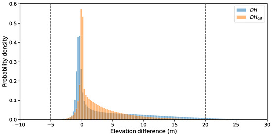
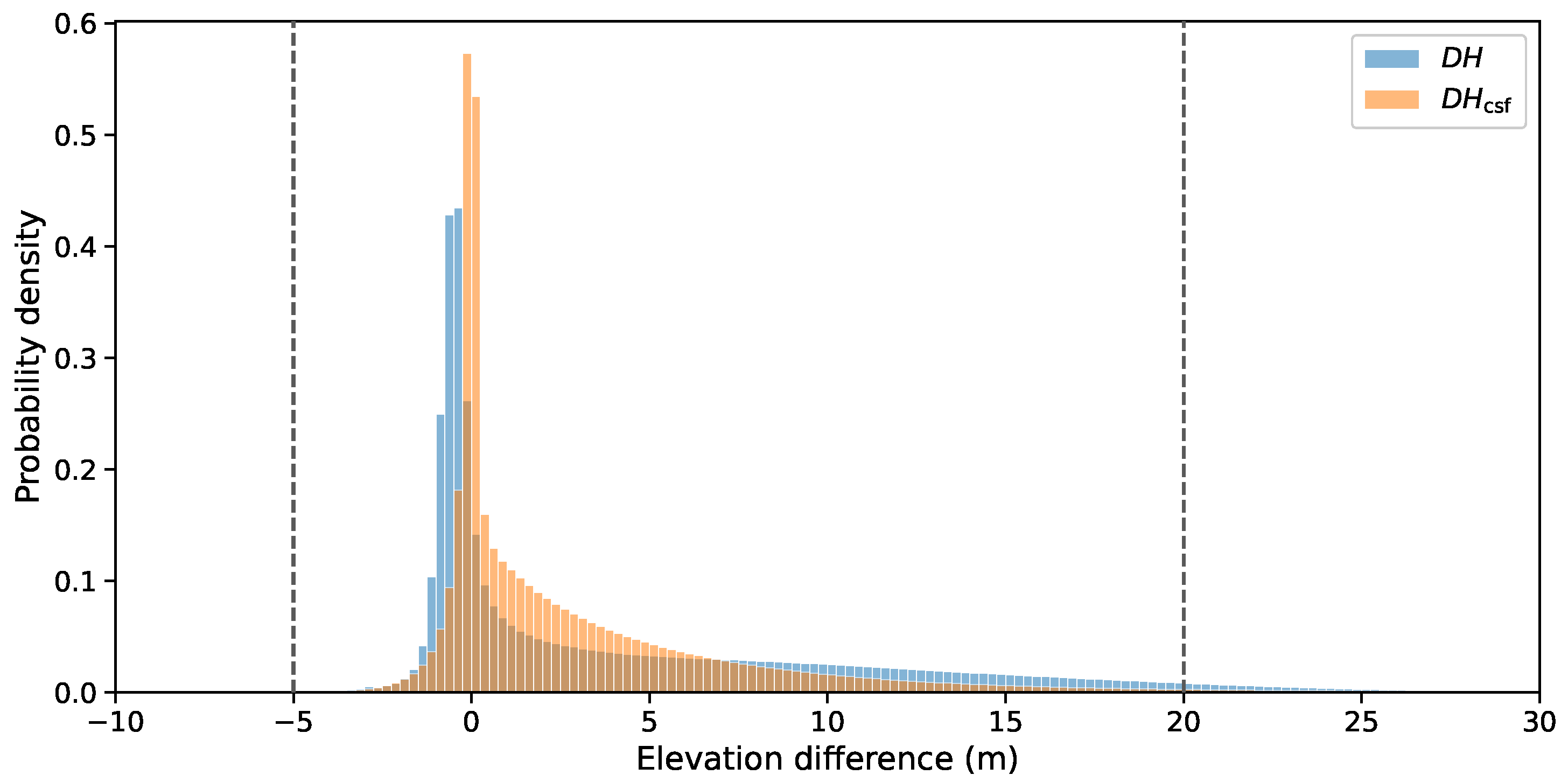
Based on the empirical distribution over the training set, the clipping interval is set to $[a,b]=[-5,20]$ m. This range is used to stabilize residual normalization and covers the dominant residual values observed in the training data. It should not be interpreted as a universal bound for DSM-to-DTM height differences. Residuals outside this interval are clipped before normalization, and the same range is used when converting the normalized network output back to meters.

The final model input is defined as

$$\mathbf{X}=\mathrm{Concat}\left({\mathrm{DSM}}_{\mathrm{norm}},{\mathrm{DH}}_{\mathrm{csf},\mathrm{norm}},G_{\mathrm{csf}},S,sin\theta ,cos\theta ,{\kappa }_{\mathrm{prof},\mathrm{norm}},{\kappa }_{\mathrm{plan},\mathrm{norm}},R_{\mathrm{norm}}\right).$$

(8)

Figure 2 shows the residual-value range used to set the fixed clipping interval in Equation (6).

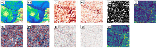
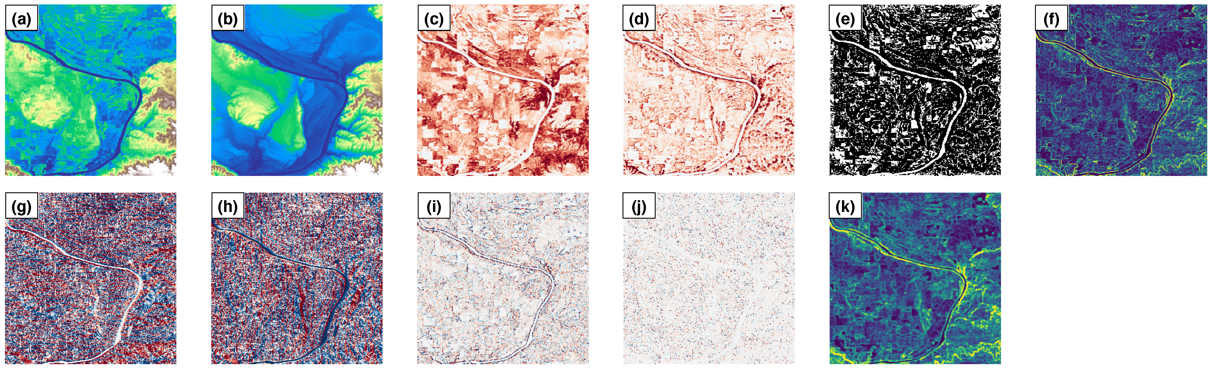
Thus, $\mathbf{X}$ contains the normalized DSM, two CSF prior channels, and six DSM-derived terrain features. The supervision target used during training is the normalized residual ${\mathrm{DH}}_{\mathrm{norm}}$. Accordingly, among the quantities shown in Figure 3, panels (a,d–k) correspond to the model inputs after preprocessing, panel (c) corresponds to the supervision target before normalization, and panel (b) is the reference DTM used for supervision, evaluation, and visual comparison.

2.3. Residual Learning Framework

The proposed framework predicts the height difference $\mathrm{DH}$ instead of absolute terrain elevation. The predicted residual is then subtracted from the input DSM to reconstruct the terrain surface.

At inference time, the model uses the COP DSM together with CSF priors and terrain features derived from that DSM. In the present implementation, inference is conducted on the same 30 m grid structure used during training and evaluation. These channels are concatenated into the multi-channel input tensor in Equation (8). The network predicts the normalized residual $\widehat{{\mathrm{DH}}_{\mathrm{norm}}}$, which is denormalized to recover $\widehat{\mathrm{DH}}$ in meters:

$$\widehat{\mathrm{DH}}=(b-a)\widehat{{\mathrm{DH}}_{\mathrm{norm}}}+a.$$

(9)

The reconstructed terrain surface is then obtained as

$$\widehat{\mathrm{DTM}}=\mathrm{DSM}-\widehat{\mathrm{DH}}.$$

(10)

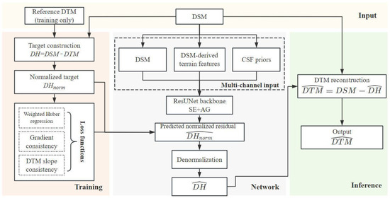
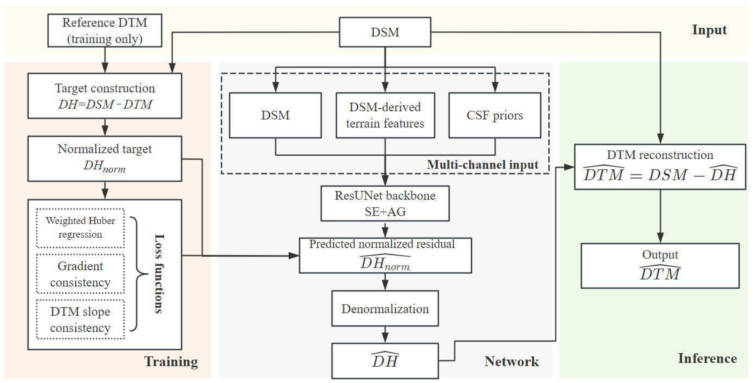
Figure 4 summarizes the overall framework.

Network Architecture

A residual U-Net (ResUNet) backbone is adopted as a practical multiscale predictor for the residual learning task, following widely used encoder–decoder and residual learning designs in dense prediction and recent terrain modeling studies [14,15,16,17,30,37,38]. The number of input channels is $C=9$, corresponding to the DSM, the CSF-derived prior channels, and the DSM-derived terrain features. The network contains four encoder stages, four decoder stages, and a bottleneck layer. Residual blocks are used throughout the backbone, together with Group Normalization and ReLU activations [39]. Squeeze-and-excitation modules are used for channel recalibration [40], and attention gates are applied in decoder skip connections to suppress irrelevant local responses.

The network output is constrained to $[0,1]$ by a Sigmoid activation:

$$\widehat{{\mathrm{DH}}_{\mathrm{norm}}}=\sigma \left(f_{\theta }\left(\mathbf{X}\right)\right),$$

(11)

where $\mathbf{X}$ denotes the multi-channel input tensor and $f_{\theta }$ is the backbone mapping. This output parameterization is consistent with the fixed-range normalization of $\mathrm{DH}$ described in Section 2.2.4.

2.4. Loss Functions and Optimization

The training objective is designed to balance residual accuracy and terrain structure. All loss terms are computed only at locations where the corresponding quantities are defined. A Huber loss is used as the primary regression term [41]:

$${\rho }_{\beta }\left(e\right)=\left\{\begin{array}{cc}{\displaystyle \frac{e^2}{2\beta }},\hfill & \left|e\right|<\beta ,\hfill \\ \left|e\right|-{\displaystyle \frac{\beta }{2}},\hfill & \mathrm{otherwise},\hfill \end{array}\right.$$

(12)

where

$$e=\widehat{{\mathrm{DH}}_{\mathrm{norm}}}-{\mathrm{DH}}_{\mathrm{norm}}.$$

(13)

To place greater emphasis on regions with larger residual magnitude, such as tall vegetation and other high-residual surface components, a tail-weight term is applied during training:

$$W=\mathrm{clip}\left(1+\alpha {\left(\frac{\left|\mathrm{DH}\right|}{h_0}\right)}^p,1,W_{max}\right).$$

(14)

The resulting weighted Huber loss is

$${\mathcal{L}}_{\mathrm{hub}}^w={\displaystyle \frac{\sum {\rho }_{\beta }\left(e_{i,j}\right)W_{i,j}}{\sum W_{i,j}+\epsilon }}.$$

(15)

To reduce edge blurring in the correction field, a gradient consistency term is imposed on $\mathrm{DH}$ in meters [14,15]:

$${\mathcal{L}}_{\mathrm{grad}}={\displaystyle \frac{\sum |{\nabla }_x\widehat{\mathrm{DH}}-{\nabla }_x\mathrm{DH}{|}_{i,j}+\sum |{\nabla }_y\widehat{\mathrm{DH}}-{\nabla }_y\mathrm{DH}{|}_{i,j}}{N_x+N_y+\epsilon }},$$

(16)

where $N_x$ and $N_y$ denote the numbers of valid finite-difference locations in the x and y directions, respectively.

Because the final product is the DTM, a slope-consistency term is further imposed in reconstructed DTM space [15,17]:

$${\mathcal{L}}_{\mathrm{slope}}={\displaystyle \frac{\sum |\mathrm{slope}\left(\widehat{\mathrm{DTM}}\right)-\mathrm{slope}\left(\mathrm{DTM}\right){|}_{i,j}}{N_{\mathrm{slope}}+\epsilon }},$$

(17)

where $N_{\mathrm{slope}}$ denotes the number of pixels at which DTM slope can be computed.

The final objective is

$$\mathcal{L}={\mathcal{L}}_{\mathrm{hub}}^w+{\lambda }_{\mathrm{grad}}{\mathcal{L}}_{\mathrm{grad}}+{\lambda }_{\mathrm{slope}}{\mathcal{L}}_{\mathrm{slope}}.$$

(18)

In the final model, $\beta =0.02$, $h_0=3.0$ m, $p=2$, $\alpha =1.0$, and $W_{max}=6.0$. The loss weights are set to ${\lambda }_{\mathrm{grad}}=0.10$ and ${\lambda }_{\mathrm{slope}}=0.02$.

Optimization is performed with AdamW [42] using an initial learning rate of $2\times {10}^{-4}$, a batch size of 4, and 100 training epochs. A warmup+cosine learning rate schedule is used [43], and gradient clipping with a maximum norm of $1.0$ is applied for stability [44]. All experiments were conducted on a workstation equipped with an Intel Core i5-12600K CPU, an NVIDIA GeForce RTX 4070 Ti SUPER GPU, and 32 GB RAM. The model was implemented in Python using PyTorch version 2.7.0. CSF priors were generated using the CNES open-source Bulldozer tool (bulldozer-dtm version 1.3.1).

2.5. Evaluation Metrics and Experimental Protocol

2.5.1. Evaluation Metrics

All evaluation metrics are computed at pixels where both the reconstructed DTM and the reference DTM are available. Unless otherwise stated, all errors are reported in meters.

We report MAE, RMSE, Bias, NMAD, P99, and Recall@5m. These metrics characterize overall accuracy, systematic bias, robust central dispersion, upper-tail error, and threshold-based accuracy, respectively [45,46]. Let N denote the number of evaluated pixels. The reported metrics are defined as

$$\begin{array}{cc}\hfill \mathrm{MAE}& ={\displaystyle \frac{1}{N}}\sum \left|{\widehat{\mathrm{DTM}}}_{i,j}-{\mathrm{DTM}}_{i,j}\right|,\hfill \\ \hfill \mathrm{RMSE}& =\sqrt{{\displaystyle \frac{1}{N}}\sum {\left({\widehat{\mathrm{DTM}}}_{i,j}-{\mathrm{DTM}}_{i,j}\right)}^2},\hfill \\ \hfill \mathrm{Bias}& ={\displaystyle \frac{1}{N}}\sum \left({\widehat{\mathrm{DTM}}}_{i,j}-{\mathrm{DTM}}_{i,j}\right),\hfill \\ \hfill \mathrm{NMAD}& =1.4826·\mathrm{median}\left(\left|e-\mathrm{median}\left(e\right)\right|\right),\hfill \\ \hfill \mathrm{P}99& ={\mathrm{percentile}}_{99}\left(\left\{\left|{\widehat{\mathrm{DTM}}}_{i,j}-{\mathrm{DTM}}_{i,j}\right|\right\}\right),\hfill \\ \hfill \mathrm{Recall}@5\mathrm{m}& ={\displaystyle \frac{1}{N}}\sum \mathbb{I}\left(\left|{\widehat{\mathrm{DTM}}}_{i,j}-{\mathrm{DTM}}_{i,j}\right|\le 5\right).\hfill \end{array}$$

(19)

Here, e in the NMAD expression denotes the set of DTM elevation errors over all evaluated pixels.

Among these metrics, NMAD and P99 complement mean-based error measures by capturing robust dispersion and upper-tail behavior, both of which are commonly used in DEM accuracy assessment [45,46].

2.5.2. Data Split and Comparison Protocol

For the study regions, the aligned data are divided into training, validation, and study region test subsets using a fixed random seed and a 70%/15%/15% split. Tile extraction is then carried out independently within each subset using the procedure described in Section 2.2.1. This study region split is used for model development, controlled comparison, and ablation analysis.

In addition, Arkansas (AR) is reserved as a held-out region for out-of-region evaluation. AR is excluded from model training, hyperparameter tuning, and model selection, and is used only after the model configuration has been fixed.

Public products, including FABDEM and FathomDEM [3,4], are evaluated as off-the-shelf surfaces after applying the same alignment and vertical-datum conversion used for the proposed method.

2.5.3. Ablation Design

Four ablation groups are defined to analyze the effects of DSM normalization, input channel composition, terrain feature groups, and loss configuration. The final model uses per-tile DSM normalization, DSM + CSF priors + DSM-derived terrain features as input, and the full loss in Equation (18). Unless otherwise stated, the supervision target $\mathrm{DH}$ and the prior channel ${\mathrm{DH}}_{\mathrm{csf}}$ always use the fixed-range clipping and normalization defined in Equations (6) and (7).

• DSM normalization. Two settings are compared for the DSM input channel: global min–max normalization and per-tile min–max normalization.
• Input channel composition. Three settings are compared: DSM only; DSM + CSF priors; and DSM + CSF priors + terrain features.
• Terrain feature groups. To further examine the contribution of individual DSM-derived terrain feature groups, one feature group is removed at a time from the full input configuration. The evaluated groups include slope, aspect encoding, curvature features, and local relief. In each case, the DSM input, CSF priors, network architecture, and loss configuration are kept unchanged.
• Loss components. Three settings are compared: weighted Huber only; weighted Huber + gradient consistency; and the full loss including DTM-slope consistency.

3. Results

This section presents comparisons with public DEM products, ablation results, held-out-region evaluation, stratified analyses, and representative qualitative examples. Unless otherwise stated, all metrics are computed at pixels where both the evaluated surface and the reference DTM are available.

3.1. Comparison with Public DEM Products and Baselines

3.1.1. Compared Methods and Evaluation Setup

The proposed method is compared on the study region test split against several publicly available DEM products and baseline methods under a unified evaluation setup. The compared methods include the COP DSM [27], CSF implemented with Bulldozer [20,36], and two public terrain correction products, FABDEM [3] and FathomDEM [4]. For comparability, all products are aligned to the same target grid and vertical datum before evaluation, and all metrics are computed over the same set of valid comparison pixels (Section 2.5.1). Evaluation on the geographically separate held-out region AR is reported separately in Section 3.3.

3.1.2. Error Characteristics of the Compared Products

Table 2. Comparison with public DEM products and baseline methods on the study region test split (meters). Downward arrows indicate metrics for which lower values are better, upward arrows indicate metrics for which higher values are better, and bold values indicate the best performance in each column.

Method	MAE ↓	RMSE ↓	Bias	NMAD ↓	P99 ↓	Recall@5m ↑
COP DSM	4.8217	7.7891	4.2982	2.8094	24.1875	0.6650
CSF (Bulldozer)	3.5466	5.8235	1.1331	2.4239	21.1875	0.7640
FABDEM	2.2096	3.5901	0.0196	1.3862	12.8875	0.8645
FathomDEM	1.0445	1.6969	-0.2783	0.6745	6.4125	0.9773
Proposed method	0.8538	1.4697	0.0309	0.6004	5.5875	0.9855

shows that the COP DSM has a large positive bias relative to the reference DTM, consistent with the retention of above-ground height contributions in public global DEM products, particularly vegetation-related signals in forested landscapes [2,3,27,28]. This broad upward offset is reflected in large overall and upper-tail errors. CSF implemented with Bulldozer reduces part of this offset, indicating that geometric filtering removes a substantial portion of the non-ground signal, but its NMAD and P99 remain relatively high. FABDEM and FathomDEM further contract the error distribution and provide much closer approximations to bare-earth terrain in this comparison.

3.1.3. Performance of the Proposed Method

The proposed method gives the best overall performance among the compared methods. Relative to FathomDEM, it improves MAE, RMSE, NMAD, P99, and Recall@5m while keeping bias close to zero. Relative to the COP DSM, the improvement is much larger, indicating substantial reduction in both the overall error level and the upper tail of the error distribution.

3.1.4. Qualitative Comparison

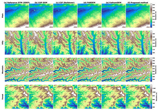
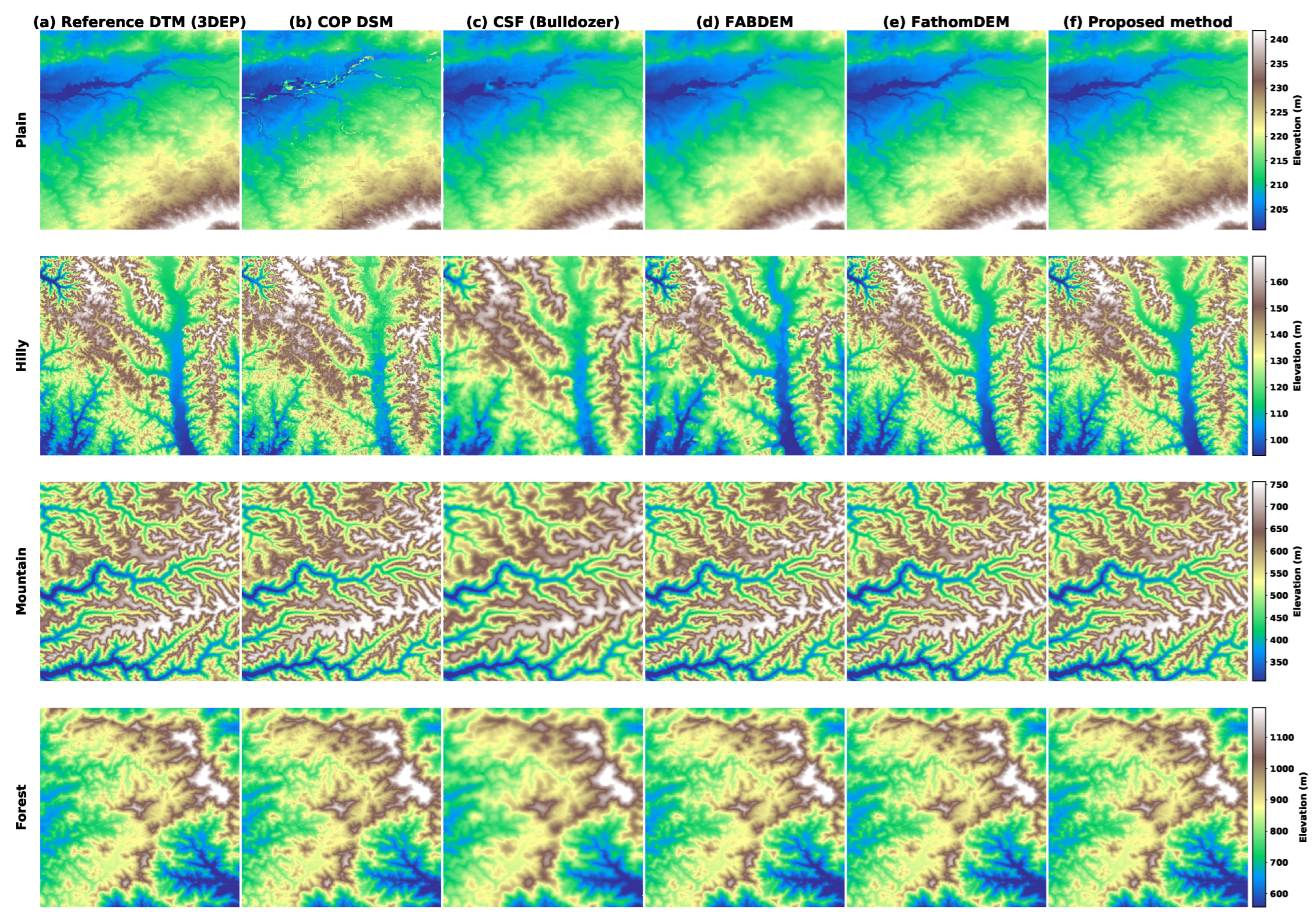
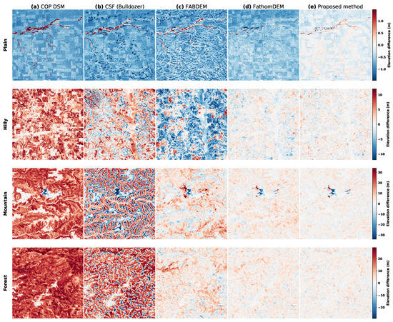
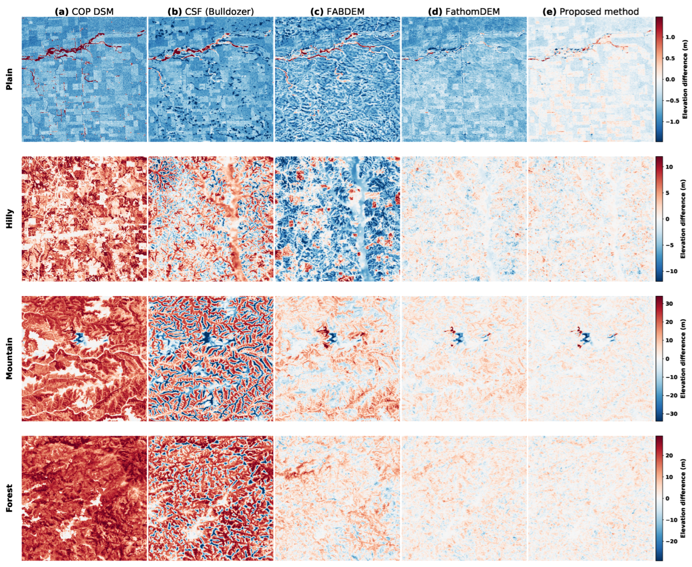
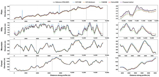
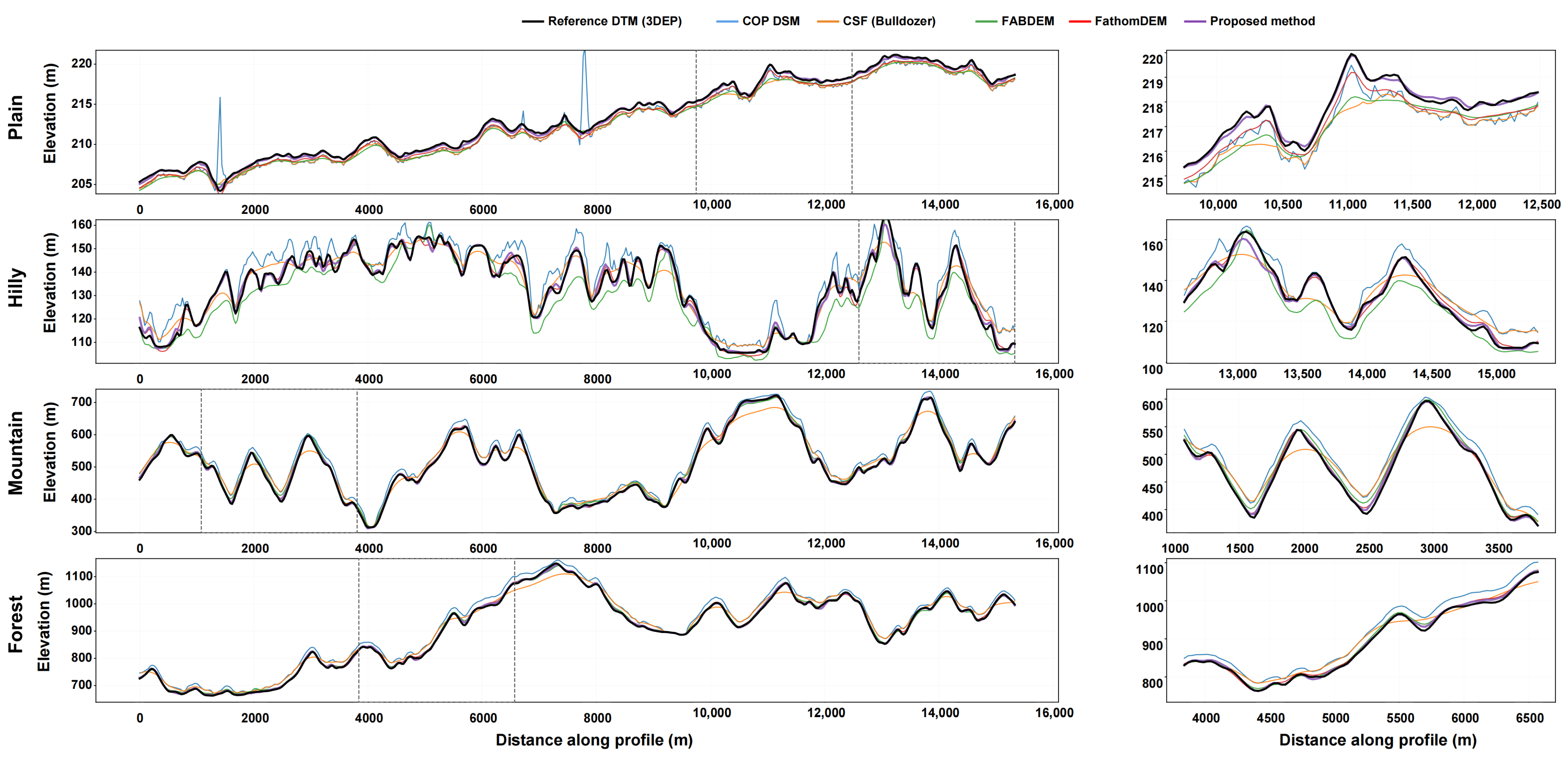
Figure 5, Figure 6 and Figure 7 compare reconstructed terrain surfaces, error maps, and representative elevation profiles for plain, hilly, mountain, and forest settings.

Across these examples, the COP DSM retains visible above-ground artifacts and local surface uplift. CSF implemented with Bulldozer removes part of this effect, but local distortions remain in more complex terrain. FABDEM and FathomDEM recover the broad terrain pattern more closely, although differences remain in local slope transitions and residual texture. In most illustrated cases, the proposed method is visually closest to the reference DTM and leaves fewer localized residual artifacts.

The error maps and profiles show the same tendency. The proposed method leaves weaker structured residuals than the compared products and follows valley-bottom variations, peak positions, and slope transitions more closely. In the mountain and forest examples, differences among the best performing methods become smaller at broad scale, although the proposed method still follows the reference profile more closely in the zoomed segments.

3.2. Ablation Study

Following the four ablation groups defined in Section 2.5.3, this subsection examines the effects of DSM normalization, input channel composition, terrain feature groups, and loss configuration under otherwise fixed training and evaluation settings. The final adopted configuration corresponds to the proposed method reported in Table 2.

3.2.1. Ablation A: DSM Normalization

Table 3. Ablation on DSM normalization strategies on the study region test split. The proposed method uses per-tile min–max normalization for DSM. Downward arrows indicate metrics for which lower values are better, upward arrows indicate metrics for which higher values are better, and bold values indicate the best performance in each column.

Normalization	MAE ↓	RMSE ↓	Bias	NMAD ↓	P99 ↓	Recall@5m ↑
Global	0.8724	1.5038	−0.0147	0.6216	5.9375	0.9847
Per-tile (Proposed method)	0.8538	1.4697	0.0309	0.6004	5.5875	0.9855

compares global min–max normalization and per-tile min–max normalization for the DSM elevation channel.

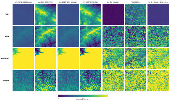
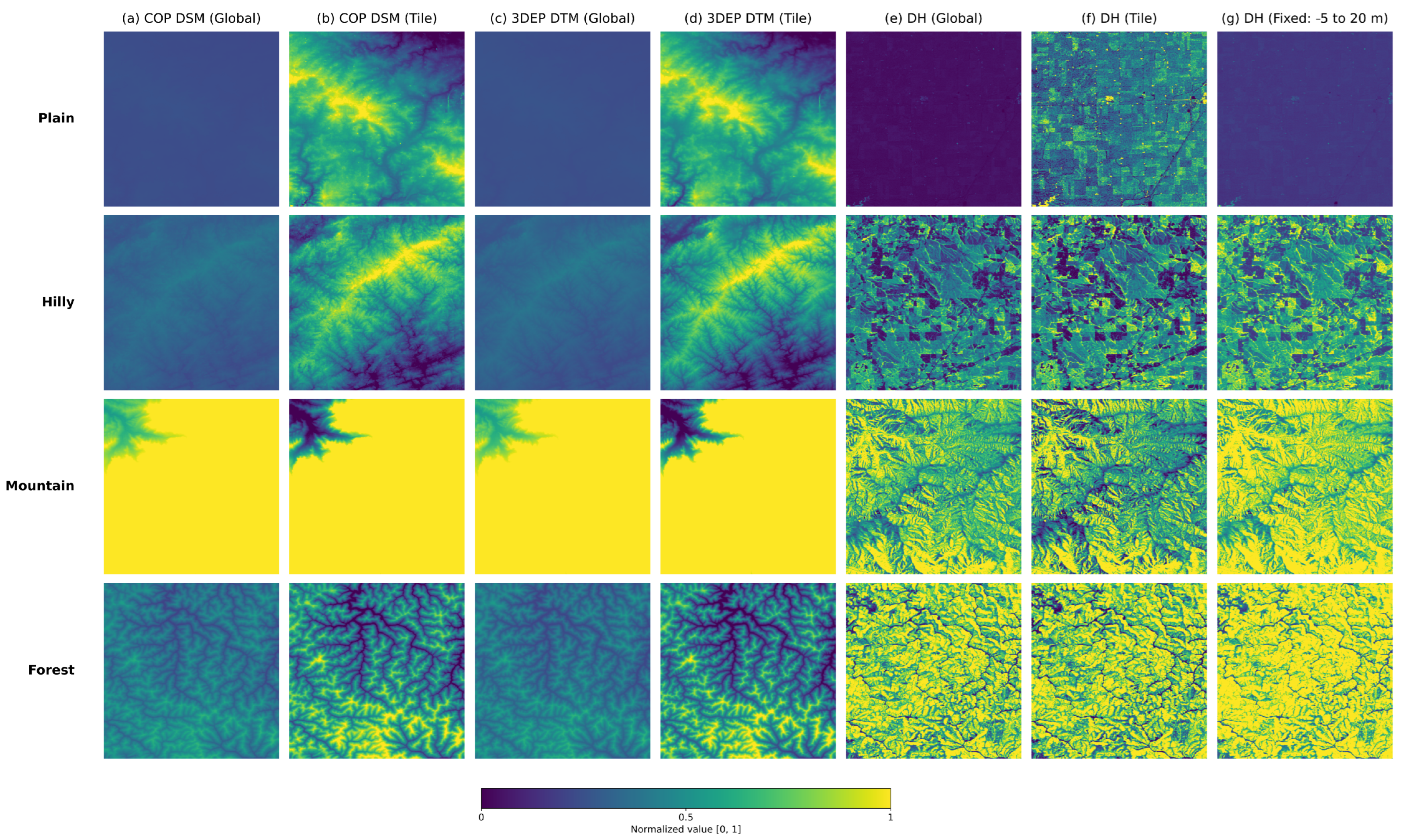
This result suggests that per-tile normalization provides a more suitable representation of local elevation contrast for the DSM input. When the normalization range is estimated over a larger spatial domain, contrast within an individual tile becomes more compressed, whereas per-tile min–max normalization preserves local structural variation more clearly. This behavior is illustrated by the representative examples in Figure 8. By contrast, the residual target $\mathrm{DH}$ is treated as a quantity that should remain on a controlled numeric scale across training and prediction, which motivates the fixed-range normalization used for $\mathrm{DH}$ and ${\mathrm{DH}}_{\mathrm{csf}}$.

3.2.2. Ablation B: Input Channel Composition

Table 4. Ablation on input channel composition on the study region test split. The proposed method uses DSM + CSF priors + terrain features. Downward arrows indicate metrics for which lower values are better, upward arrows indicate metrics for which higher values are better, and bold values indicate the best performance in each column.

Inputs	MAE ↓	RMSE ↓	Bias	NMAD ↓	P99 ↓	Recall@5m ↑
DSM only	1.2151	2.0827	0.0998	0.8228	8.0375	0.9589
DSM + CSF priors (${\mathrm{DH}}_{\mathrm{csf}}$, $G_{\mathrm{csf}}$)	0.9610	1.6173	0.0715	0.7042	6.0625	0.9811
DSM + CSF priors + terrain features (Proposed method)	0.8538	1.4697	0.0309	0.6004	5.5875	0.9855

summarizes the incremental addition of input channels, starting from the DSM-only setting, then adding the CSF priors, and finally adding the DSM-derived terrain features.

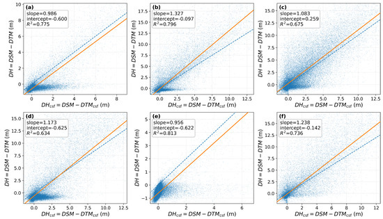
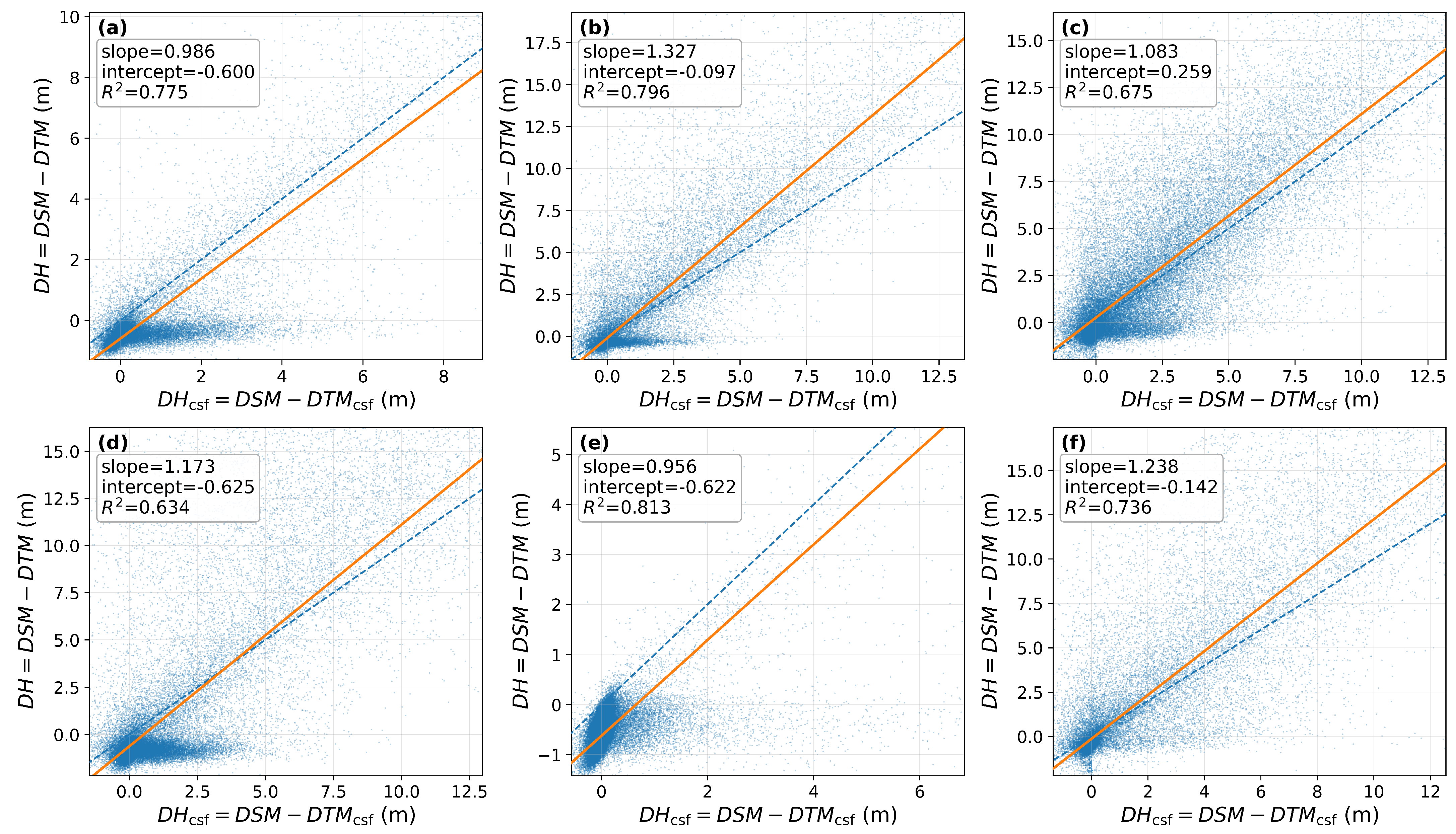
The largest single improvement comes from the CSF priors. Relative to the DSM-only setting, their addition substantially reduces overall, robust, and upper-tail errors, indicating that the CSF-derived residual prior and ground mask provide strong coarse guidance for identifying where above-ground contributions are likely to occur. This gain is obtained using a consistent Bulldozer configuration across all study regions, with the slope-related setting derived from the input DSM rather than from the reference DTM. However, the CSF prior is not a direct substitute for the target. As shown in Figure 9, the correspondence between ${\mathrm{DH}}_{\mathrm{csf}}$ and the reference $\mathrm{DH}$ is clearly positive but far from one-to-one.

Adding DSM-derived terrain features provides a further improvement across all reported metrics. The additional gain is smaller than that obtained from the CSF priors, suggesting that the two input groups play different roles. The CSF priors provide the main coarse correction signal, whereas the terrain feature channels contribute local refinement.

The relative contributions of the individual terrain feature groups are examined in the following feature-group ablation.

3.2.3. Ablation C: Terrain Feature Groups

To further examine which DSM-derived terrain features contribute most to the final model, an additional feature-group ablation is conducted. Starting from the full input configuration, one terrain feature group is excluded at a time while keeping the DSM input, CSF priors, network architecture, and loss configuration unchanged. This experiment evaluates the relative contribution of slope, aspect encoding, curvature features, and local relief within the terrain feature channels.

Table 5. Feature-group ablation within the DSM-derived terrain feature channels on the study region test split. Each setting removes one terrain feature group from the full model while keeping the DSM input, CSF priors, network architecture, and loss configuration unchanged. ΔMAE and ΔRMSE are computed relative to the full terrain feature setting. Downward arrows indicate metrics for which lower values are better, upward arrows indicate metrics for which higher values are better, and bold text indicates the adopted full model.

Terrain Feature Setting	MAE ↓	ΔMAE	RMSE ↓	ΔRMSE	NMAD ↓	P99 ↓	Recall@5m ↑
Full terrain features (Proposed method )	0.8538	–	1.4697	–	0.6004	5.5875	0.9855
Excluding aspect encoding ($sin\theta ,cos\theta$)	0.8610	0.0072	1.4810	0.0113	0.6070	5.6400	0.9853
Excluding curvature features (${\kappa }_{\mathrm{prof}},{\kappa }_{\mathrm{plan}}$)	0.8710	0.0172	1.5000	0.0303	0.6160	5.7500	0.9850
Excluding slope (S)	0.8825	0.0287	1.5200	0.0503	0.6300	5.8500	0.9844
Excluding local relief (R)	0.8950	0.0412	1.5450	0.0753	0.6425	5.9750	0.9840
Excluding all terrain features	0.9610	0.1072	1.6173	0.1476	0.7042	6.0625	0.9811

shows that removing any terrain feature group degrades performance relative to the full configuration, although the magnitude of degradation differs among feature groups. The largest performance decrease is observed when local relief is excluded, followed by slope and curvature features, whereas excluding aspect encoding causes the smallest change. This pattern suggests that local relief and slope provide stronger local geometric cues for residual height prediction, while aspect encoding contributes more modestly under the present study conditions.

The results also show that excluding all terrain features causes a much larger degradation than removing any single feature group. This indicates that the terrain feature channels provide complementary information: no individual group alone explains the full gain, but their combined use improves local refinement beyond the DSM and CSF priors.

3.2.4. Ablation D: Loss Components

Table 6. Ablation on loss components on the study region test split. The proposed method uses all three loss terms. Downward arrows indicate metrics for which lower values are better, upward arrows indicate metrics for which higher values are better, bold text indicates the adopted loss setting, and bold values indicate the best performance in each column.

Loss Setting	MAE ↓	RMSE ↓	Bias	NMAD ↓	P99 ↓	Recall@5m ↑
${\mathcal{L}}_{\mathrm{hub}}^w$ only	0.9200	1.5644	−0.0105	0.6745	5.8625	0.9830
${\mathcal{L}}_{\mathrm{hub}}^w+{\lambda }_{\mathrm{grad}}{\mathcal{L}}_{\mathrm{grad}}$	0.8852	1.5218	0.0031	0.6301	5.7125	0.9843
${\mathcal{L}}_{\mathrm{hub}}^w+{\lambda }_{\mathrm{grad}}{\mathcal{L}}_{\mathrm{grad}}+{\lambda }_{\mathrm{slope}}{\mathcal{L}}_{\mathrm{slope}}$ (Proposed method )	0.8538	1.4697	0.0309	0.6004	5.5875	0.9855

reports the effect of progressively adding the gradient consistency and DTM-space slope consistency terms to the weighted Huber loss.

Both additional loss terms improve the results relative to the weighted Huber baseline, and the full loss yields the best performance across all reported metrics. Compared with the input channel ablation, the loss-term ablation reflects a different type of contribution. The terrain-aware loss terms do not provide the main coarse correction, but they consistently refine the predicted residual field and the reconstructed terrain surface once a stronger input representation is available.

3.3. Held-Out Region Evaluation

3.3.1. Study Region and Held-Out Region Performance

Table 7. Overall performance of the proposed method on the study region test split and the held-out region AR (meters). Downward arrows indicate metrics for which lower values are better, and upward arrows indicate metrics for which higher values are better.

Dataset	MAE ↓	RMSE ↓	Bias	NMAD ↓	P99 ↓	Recall@5m ↑
Study region test split	0.8538	1.4697	0.0309	0.6004	5.5875	0.9855
Held-out region AR	0.8706	1.5116	0.0380	0.6072	5.6875	0.9845

reports the overall performance of the proposed method on the study region test split and on the geographically separate held-out region AR.

3.3.2. Held-Out Region Results

The difference between the study region test split and the held-out AR evaluation is small across all reported metrics. For example, MAE increases from 0.8538 to 0.8706 and RMSE from 1.4697 to 1.5116, while bias, NMAD, P99, and Recall@5m remain similarly close. These results suggest that the learned mapping transfers reasonably well to the geographically separate held-out region under the present evaluation setting.

3.4. Stratified Performance Analysis

To examine how performance varies with terrain and vegetation conditions, stratified analyses are conducted by elevation, slope, and canopy height. These grouping variables are used only for analysis and are not provided as model inputs. Therefore, this section focuses on how reconstruction accuracy changes across topographic and canopy height gradients, and then presents a representative local detail comparison to illustrate fine-scale reconstruction behavior.

3.4.1. Elevation-Stratified Performance

Table 8. Elevation-stratified error statistics by elevation bins (meters). Bold values indicate the best performance within each elevation bin.

Elevation Bin (m)	Method	Bias	MAE	RMSE	NMAD	P99
$[0,200)$	COP DSM	4.3039	4.8212	6.9153	2.5373	19.5289
$[0,200)$	CSF (Bulldozer)	1.9557	3.1923	4.5728	1.9915	14.0259
$[0,200)$	FABDEM	0.0025	2.2486	3.2806	1.5100	10.7969
$[0,200)$	FathomDEM	−0.2786	0.8993	1.3150	0.6509	4.3611
$[0,200)$	Proposed method	0.0200	0.7845	1.2014	0.6387	4.1161
$[200,500)$	COP DSM	3.7418	4.2948	6.0262	2.5350	16.5400
$[200,500)$	CSF (Bulldozer)	0.3749	3.3791	4.6562	2.8385	13.9462
$[200,500)$	FABDEM	0.0331	2.0015	2.8220	1.5750	8.8489
$[200,500)$	FathomDEM	−0.3179	1.0130	1.3903	0.7653	4.3421
$[200,500)$	Proposed method	0.0210	0.8192	1.2157	0.7384	4.0668
$[500,1000)$	COP DSM	11.2476	11.4584	13.5323	5.9374	27.0429
$[500,1000)$	CSF (Bulldozer)	1.8268	9.4473	12.0317	9.6385	31.1531
$[500,1000)$	FABDEM	0.0385	4.5249	5.8724	4.6326	15.7144
$[500,1000)$	FathomDEM	0.1939	2.3615	3.1423	2.4437	9.0505
$[500,1000)$	Proposed method	0.2981	2.0626	2.7972	2.1166	8.3545
$[1000,2000)$	COP DSM	16.2191	16.2655	17.7765	6.6489	31.3557
$[1000,2000)$	CSF (Bulldozer)	3.3898	13.4152	16.3882	15.1299	42.4347
$[1000,2000)$	FABDEM	−0.0101	5.2575	6.5404	5.8574	16.4487
$[1000,2000)$	FathomDEM	0.4780	3.1762	4.0442	3.7153	10.8175
$[1000,2000)$	Proposed method	0.2757	2.6083	3.3989	3.0143	9.6988

reports error statistics by elevation bin. Across all elevation bins considered here, the proposed method maintains the lowest MAE and RMSE among the compared methods. Absolute error increases with elevation for all methods, indicating increasing difficulty at higher elevations. At the same time, the proposed method retains its advantage over FathomDEM throughout the represented elevation bins, and this advantage becomes larger in the higher-elevation ranges included in the present dataset.

For the proposed method itself, both MAE and RMSE increase substantially from the lowest to the highest elevation bin. Higher-elevation settings therefore remain a clear source of difficulty, even though the relative ranking among methods is preserved.

3.4.2. Slope-Stratified Performance

Table 9. Slope-stratified error statistics by slope bins (meters). Bold values indicate the best performance within each slope bin.

Slope Bin (deg)	Method	Bias	MAE	RMSE	NMAD	P99
$[0,5)$	COP DSM	2.0997	2.8138	4.5019	1.1727	15.0555
$[0,5)$	CSF (Bulldozer)	0.3905	2.3767	3.5177	1.6284	11.4862
$[0,5)$	FABDEM	−0.2818	1.5344	2.2916	1.0046	7.9035
$[0,5)$	FathomDEM	−0.3473	0.7179	1.0197	0.5003	3.3205
$[0,5)$	Proposed method	−0.0250	0.5645	0.8848	0.4658	3.1210
$[5,10)$	COP DSM	6.5294	6.7454	8.6238	5.1302	20.5213
$[5,10)$	CSF (Bulldozer)	2.1503	4.6197	6.1563	3.4140	17.2721
$[5,10)$	FABDEM	0.1496	2.9055	3.9742	2.2557	11.8794
$[5,10)$	FathomDEM	−0.2487	1.2501	1.7216	0.9720	5.3693
$[5,10)$	Proposed method	0.0743	1.1250	1.5930	0.9471	5.1238
$[10,15)$	COP DSM	8.9812	9.1188	10.8304	5.6488	22.7890
$[10,15)$	CSF (Bulldozer)	2.7409	5.9390	7.6575	3.5516	20.4962
$[10,15)$	FABDEM	0.6293	3.5791	4.6761	2.7181	12.9243
$[10,15)$	FathomDEM	−0.1446	1.6501	2.2196	1.1998	6.5784
$[10,15)$	Proposed method	0.1618	1.4520	1.9959	1.1408	6.1134
$[15,20)$	COP DSM	11.1441	11.2731	12.8823	5.6325	24.9497
$[15,20)$	CSF (Bulldozer)	3.0204	7.5020	9.4416	3.5390	24.3260
$[15,20)$	FABDEM	1.2847	4.2852	5.4346	2.9096	14.1501
$[15,20)$	FathomDEM	−0.0214	2.0818	2.7429	1.3654	7.8043
$[15,20)$	Proposed method	0.2228	1.7865	2.4064	1.2559	7.1276
$[20,30)$	COP DSM	13.8616	13.9944	15.5113	5.6547	27.9131
$[20,30)$	CSF (Bulldozer)	3.2418	9.3967	11.6544	3.6951	29.5140
$[20,30)$	FABDEM	2.0636	5.2028	6.4609	3.1377	16.1714
$[20,30)$	FathomDEM	0.2299	2.6472	3.4204	1.5768	9.4394
$[20,30)$	Proposed method	0.3186	2.2448	2.9695	1.4528	8.5798
$[30,45)$	COP DSM	15.9608	16.2228	17.6008	5.8505	30.0142
$[30,45)$	CSF (Bulldozer)	2.5264	9.9649	12.3863	4.6130	32.1457
$[30,45)$	FABDEM	3.3528	6.2457	7.6385	3.8490	18.4706
$[30,45)$	FathomDEM	0.3798	3.1572	4.0288	2.1403	10.8409
$[30,45)$	Proposed method	0.3802	2.6564	3.4999	2.0345	10.0190
$[45,+\infty )$	COP DSM	10.8859	14.9914	16.8134	5.4153	34.0941
$[45,+\infty )$	CSF (Bulldozer)	−7.7047	12.1746	15.2348	5.6553	38.3895
$[45,+\infty )$	FABDEM	8.1610	10.9134	12.8070	4.5670	27.0022
$[45,+\infty )$	FathomDEM	−2.7132	5.7930	7.3842	2.6930	20.1676
$[45,+\infty )$	Proposed method	−1.6840	5.2847	7.6154	2.9022	24.4163

reports error statistics by slope bin. Errors increase steadily with slope for all methods, confirming that steep terrain is a major source of difficulty in the present problem. Up to the $[30,45)$ bin, the proposed method remains better than FathomDEM in both MAE and RMSE, and its relative advantage generally becomes larger as slope increases.

In the most extreme slope bin, the pattern becomes mixed. MAE remains lower than that of FathomDEM, but RMSE, NMAD, and P99 become less favorable. This suggests that extremely steep terrain produces a small number of severe local failures that disproportionately affect squared and upper-tail metrics.

3.4.3. Canopy-Height-Stratified Performance

Table 10. Canopy-height-stratified error statistics (meters). Bold values indicate the best performance within each canopy-height bin.

Canopy Height Bin (m)	Method	Bias	MAE	RMSE	NMAD	P99
$[0,2)$	COP DSM	−0.4370	0.6120	0.7985	0.2796	1.9055
$[0,2)$	CSF (Bulldozer)	−0.8873	0.9759	1.2798	0.4791	3.8241
$[0,2)$	FABDEM	−0.4904	0.6370	0.8180	0.3950	2.0297
$[0,2)$	FathomDEM	−0.3584	0.4129	0.5203	0.2442	1.2420
$[0,2)$	Proposed method	−0.0132	0.2068	0.3300	0.2063	0.9625
$[2,5)$	COP DSM	−0.4262	0.6601	0.9049	0.3079	2.4212
$[2,5)$	CSF (Bulldozer)	−1.3429	1.4480	2.0043	0.6561	6.2750
$[2,5)$	FABDEM	−0.4565	0.6727	0.9073	0.4622	2.4082
$[2,5)$	FathomDEM	−0.3604	0.4401	0.5746	0.2748	1.4851
$[2,5)$	Proposed method	−0.0817	0.2580	0.4032	0.2217	1.2021
$[5,10)$	COP DSM	0.1735	1.0941	1.7014	0.4450	5.6269
$[5,10)$	CSF (Bulldozer)	−1.1115	1.7299	2.5340	0.8509	8.2921
$[5,10)$	FABDEM	0.0478	1.0097	1.5335	0.6056	4.8669
$[5,10)$	FathomDEM	−0.3601	0.5395	0.7399	0.3573	2.1798
$[5,10)$	Proposed method	−0.1477	0.4012	0.6229	0.3009	2.0938
$[10,20)$	COP DSM	2.4667	2.7991	4.1190	1.8846	12.9124
$[10,20)$	CSF (Bulldozer)	0.1013	2.2922	3.3892	1.7119	11.2996
$[10,20)$	FABDEM	0.1671	1.9165	2.7523	1.2905	8.9429
$[10,20)$	FathomDEM	−0.2859	0.7609	1.0482	0.6146	3.3515
$[10,20)$	Proposed method	−0.1624	0.7030	1.0189	0.6103	3.4394
$[20,30)$	COP DSM	9.1308	9.1862	10.6793	5.2368	22.3070
$[20,30)$	CSF (Bulldozer)	3.7384	5.7730	7.2864	3.9511	19.0080
$[20,30)$	FABDEM	0.0279	3.5210	4.5331	3.0921	12.2917
$[20,30)$	FathomDEM	−0.1974	1.5168	2.0234	1.3065	6.0520
$[20,30)$	Proposed method	0.2276	1.3386	1.8238	1.2118	5.6587
$[30,+\infty )$	COP DSM	17.0946	17.1205	18.1322	5.2451	29.3633
$[30,+\infty )$	CSF (Bulldozer)	6.5172	12.0780	14.2332	5.5086	31.4942
$[30,+\infty )$	FABDEM	2.0357	5.6919	6.9498	4.3753	16.4860
$[30,+\infty )$	FathomDEM	0.2126	2.8099	3.5588	2.1494	9.4675
$[30,+\infty )$	Proposed method	0.8120	2.3965	3.0981	1.9130	8.6467

shows that all methods degrade as canopy height increases, which is consistent with the larger and more variable above-ground component in taller-canopy areas. The proposed method nonetheless maintains the best MAE and RMSE across all canopy bins considered here.

For the proposed method, both MAE and RMSE increase monotonically with canopy height. The gain relative to FathomDEM is not limited to the low-canopy regime; it remains visible across all bins and is still present in the highest-canopy setting represented in this analysis.

3.4.4. Local Detail Comparison

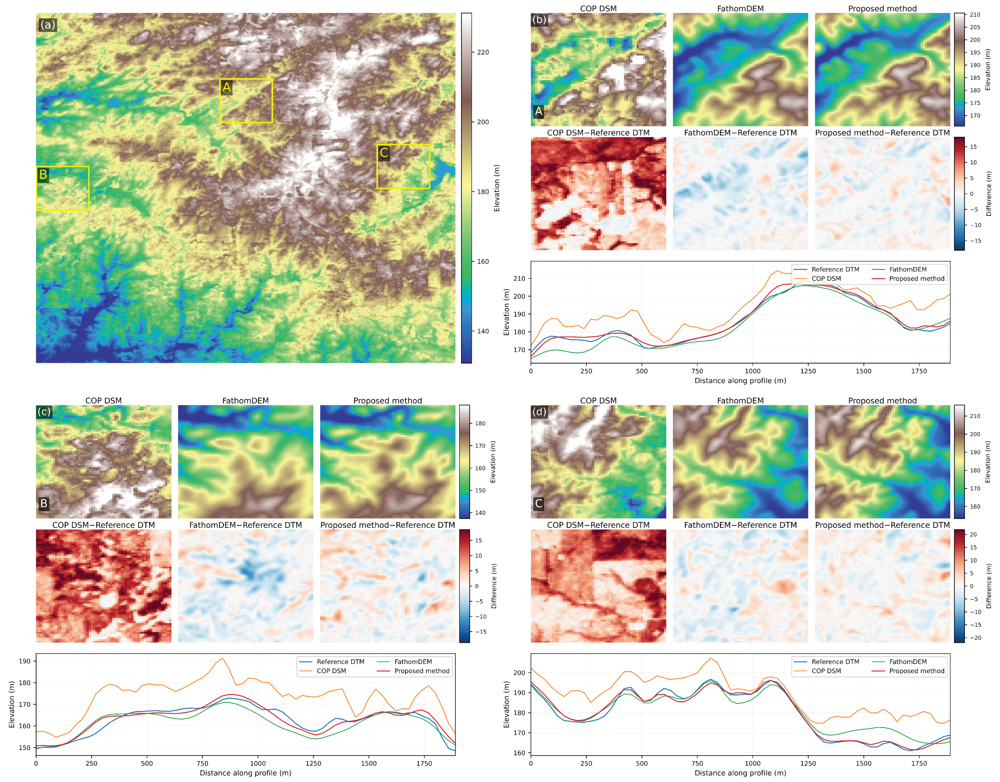
To complement the region-level and stratified statistics, a representative local-detail comparison is shown in Figure 10. The figure presents one larger context window together with several selected local patches, allowing comparison of terrain surface reconstruction, error patterns relative to the reference DTM, and profile behavior at finer spatial scale.

Figure 10 shows that both methods recover the broad terrain pattern, but differences remain in local morphology and residual structure. In the illustrated patches, the proposed method generally produces terrain surfaces that are closer to the reference DTM, with smoother removal of the broad positive offset present in the COP DSM and with less spatially organized residual error than FathomDEM.

The profile comparisons support the same interpretation. Along the representative transects, the proposed method more closely follows the reference terrain in local slope transitions, ridge–valley shape, and short-range elevation variation. These local examples are consistent with the quantitative results reported above, indicating that the gain of the proposed framework is not limited to aggregated error statistics but is also visible in fine-scale terrain reconstruction.

4. Discussion

This study examines DSM-to-DTM reconstruction in a single-source setting in which only the COP DSM is required during prediction. Within this setting, the method is designed to recover bare-earth terrain without relying on externally sourced thematic, biophysical, or image-based data layers during prediction. This distinguishes the proposed inference workflow from multi-source terrain correction products such as FABDEM and FathomDEM. The results make it possible to separate the contributions of the residual target, the DSM-derived auxiliary channels, and the terrain-aware loss design, while also identifying the conditions under which the present formulation becomes less reliable.

4.1. Residual Learning in the Single-Source Setting

A central design choice in this study is to predict the residual field $\mathrm{DH}=\mathrm{DSM}-\mathrm{DTM}$ rather than absolute terrain elevation. This is well matched to the present task because the input DSM already preserves much of the broad terrain structure, while the main uncertainty lies in the non-ground component that should be removed.

In this setting, direct DTM regression would require the model to recover both the large-scale terrain level and the local correction term from the same source. Predicting $\mathrm{DH}$ instead focuses learning on the part that differs systematically between the DSM and the reference DTM. This makes the target more closely aligned with the practical objective of DSM-to-DTM correction when no external predictors are available at inference time.

This interpretation is specific to the present problem setup. It should not be taken to mean that residual learning is always preferable to direct terrain regression, but it is a natural choice when the input surface already contains substantial terrain information.

4.2. Roles of CSF Priors, Terrain Features, and Terrain-Aware Losses

The ablation results show that different parts of the framework contribute in different ways. The largest single gain comes from the CSF-derived prior channels. This suggests that, even when generated from the DSM alone, a coarse ground estimate and its associated ground mask provide strong guidance about where the observed surface is likely to contain non-ground height. In the present framework, the CSF output is not used as the final terrain surface. Instead, it acts as a structured prior that narrows the search space of the residual-learning task.

Because the CSF priors provide the largest single gain, their parameter settings may influence the quality of the model inputs. In this study, the Bulldozer configuration is kept consistent across regions, and the adaptive maximum-slope setting is derived from the DSM of each tile rather than tuned using reference DTM data. A systematic sensitivity analysis of CSF parameters is not conducted here and remains a useful direction for future work.

The DSM-derived terrain features provide a second type of information. Their incremental gain is smaller than that of the CSF priors, but it is consistent across the reported metrics. The additional feature group ablation further shows that these terrain features do not contribute equally. Removing local relief causes the largest degradation, followed by slope and curvature features, whereas removing aspect encoding has the smallest effect. This suggests that local relief and slope provide particularly useful local geometric cues for residual height prediction, while aspect encoding contributes more modestly under the present study conditions. These channels describe neighborhood geometry that is already implicit in the DSM, but present it in a form that is easier for the network to use when separating terrain shape from above-ground structure. In this sense, the terrain features complement the CSF priors rather than replace them.

The loss design contributes at a different stage of the correction process. The weighted Huber term remains the main regression objective, while the gradient consistency and DTM-slope consistency terms constrain the spatial structure of the predicted correction and the morphology of the reconstructed terrain surface. Their quantitative gains are smaller than those introduced by the CSF priors, but they are consistent across both central and upper-tail metrics. This matches their intended role. They do not provide new information about where non-ground structure occurs, but instead regularize how that structure is removed.

Taken together, these results suggest that the performance gain comes from the combined effect of the residual target, the CSF priors, the terrain features, and the terrain-aware losses, rather than from the backbone alone.

4.3. Performance Across Different Conditions

Under the present evaluation setup, the proposed method gives the best overall results among the compared products and baselines. Relative to FathomDEM, the improvement is visible not only in MAE and RMSE, but also in NMAD, P99, and Recall@5m. Because all products are evaluated after the same alignment and vertical-datum conversion and over the same valid comparison pixels, these differences reflect performance under a common comparison setting.

The stratified analyses also show clear limits. Errors increase with elevation, slope, and canopy height for all methods, including the proposed one. This suggests that reconstruction becomes more difficult when the separation between bare-earth terrain and above-ground structure is less clearly expressed in the DSM geometry. Even so, the proposed method remains better than FathomDEM across most elevation and canopy bins, and its advantage generally increases with slope up to the $[30,45)$ bin.

The most extreme slope regime behaves differently. In the $[45,+\infty )$ bin, MAE remains lower than that of FathomDEM, whereas RMSE, NMAD, and P99 become less favorable. This pattern suggests that the main limitation is a small number of severe local failures rather than a uniform degradation across the entire bin. A related trend appears in the canopy-stratified results: the method remains competitive as canopy height increases, but absolute error still rises steadily in taller-canopy settings. In both cases, DSM geometry alone is not always sufficient to resolve the most difficult terrain–vegetation configurations.

The held-out evaluation on Arkansas should be interpreted in the same context. The small difference between the study region test split and the held-out region suggests that the learned mapping transfers reasonably well under the present spatial separation design. However, this should not be taken as evidence of broad geographic generalization, because the held-out analysis includes only one additional region within the broader study area. The Arkansas result is therefore better viewed as a useful external check than as a definitive test of cross-region generalization.

4.4. Practical Implications and Remaining Limitations

From an operational perspective, the main advantage of the framework is that inference depends on a single source dataset. All auxiliary channels used by the model are derived from the DSM itself, which reduces the burden of assembling and harmonizing external layers with different acquisition times, spatial supports, and reference systems. This is particularly relevant for large-area applications, where data matching can become a substantial part of the workflow.

At the same time, the single-source design does not eliminate preprocessing altogether. The CSF priors still need to be derived from the DSM, so the workflow is most practical when preprocessing can be performed once over a fixed area and the resulting inputs can then be reused.

Several limitations remain. First, the fixed clipping range for $\mathrm{DH}$ improves scale consistency between training and prediction, but it also limits the residual values that the model can represent. In the current implementation, residuals larger than 20 m or smaller than $-5$ m are clipped during target normalization, and the Sigmoid output followed by fixed-range denormalization restricts the predicted $\widehat{\mathrm{DH}}$ to the same interval. This design helps stabilize training for the empirical residual distribution of the present dataset, but it can compress very large residual values and may contribute to under-correction in high-residual cases.

Second, the framework is developed and evaluated on the approximately 30 m COP DSM grid. The CSF priors, terrain derivatives, local-relief calculation, and the physical footprint of the $512\times 512$ tiles are tied to this spatial resolution. Therefore, the present results should not be interpreted as evidence of direct transferability to DSMs with substantially different spatial resolutions. Applying the framework to other DSM resolutions may require recalibration of feature generation, CSF settings, and model fine-tuning or retraining.

Third, the mixed behavior in the most difficult slope and canopy regimes suggests that a purely geometry-based single-source approach has a practical limit when the DSM does not contain enough evidence to distinguish terrain from non-ground structure.

Another limitation is that this study does not include a dedicated validation over urban or building-dominated areas. Buildings are important above-ground objects in DSM-to-DTM reconstruction, but their geometric structure differs from vegetation canopies. Therefore, the current results should not be interpreted as a comprehensive validation of the model’s ability to remove building-induced elevation effects. Future work should further assess the proposed framework in urban and building-dominated environments, preferably with independent building footprint or building height information.

These observations point to several natural extensions. One is to explore adaptive residual scaling or alternative output parameterizations that preserve training stability while reducing compression of extreme $\mathrm{DH}$ values. Another is broader evaluation across regions, resolutions, and urbanization levels. A third is to test whether a limited set of additional auxiliary inputs can improve the most difficult high-residual cases without sacrificing the main practical advantage of the single-source design.

5. Conclusions

This study presents a DSM-to-DTM reconstruction framework for a setting in which inference is restricted to DSM-derived information, without requiring external auxiliary data during prediction. The method predicts the residual $\mathrm{DH}=\mathrm{DSM}-\mathrm{DTM}$ and combines the DSM with CSF-derived priors, DSM-derived terrain features, and terrain-aware loss terms to improve bare-earth reconstruction.

Under the present evaluation setup, the proposed method achieves the best overall performance among the compared methods. Relative to FathomDEM, it reduces MAE from $1.0445$ m to $0.8538$ m and RMSE from $1.6969$ m to $1.4697$ m while also improving NMAD, P99, and Recall@5m. The ablation results further show that the largest single gain comes from the CSF priors, whereas terrain features and terrain-aware losses provide additional refinement.

Performance on the held-out Arkansas region remains close to that on the study region test split, suggesting reasonable transfer under the present spatial separation design. Overall, the results indicate that effective large-area DSM-to-DTM reconstruction is feasible in the evaluated 30 m COP DSM setting with a predominantly single-source design while reducing dependence on external auxiliary data at inference time. This makes the proposed framework particularly relevant for large-area applications where external auxiliary datasets are unavailable, inconsistent, or difficult to harmonize. The method nevertheless remains less reliable in extremely steep terrain, difficult vegetated settings, and cases with very large values of $\mathrm{DH}$, particularly where residual heights exceed the adopted target range. Further evaluation is still needed for urban or building-dominated areas and for DSMs with spatial resolutions different from the 30 m COP DSM used here.

References

- Guth, P.L.; Van Niekerk, A.; Grohmann, C.H.; Muller, J.P.; Hawker, L.; Florinsky, I.V.; Gesch, D.; Reuter, H.I.; Herrera-Cruz, V.; Riazanoff, S.; et al. Digital Elevation Models: Terminology and Definitions. Remote Sens. 2021, 13, 3581. [Google Scholar] [CrossRef] [Scilit]
- O’Loughlin, F.E.; Paiva, R.C.D.; Durand, M.; Alsdorf, D.E.; Bates, P.D. A Multi-Sensor Approach towards a Global Vegetation Corrected SRTM DEM Product. Remote Sens. Environ. 2016, 182, 49–59. [Google Scholar] [CrossRef] [Scilit]
- Hawker, L.; Uhe, P.; Paulo, L.; Sosa, J.; Savage, J.; Sampson, C.; Neal, J. A 30 m Global Map of Elevation with Forests and Buildings Removed. Environ. Res. Lett. 2022, 17, 024016. [Google Scholar] [CrossRef] [Scilit]
- Uhe, P.; Lucas, C.; Hawker, L.; Brine, M.; Wilkinson, H.; Cooper, A.; Saoulis, A.A.; Savage, J.; Sampson, C. FathomDEM: An Improved Global Terrain Map Using a Hybrid Vision Transformer Model. Environ. Res. Lett. 2025, 20, 034002. [Google Scholar] [CrossRef] [Scilit]
- Meng, X.; Currit, N.; Zhao, K. Ground Filtering Algorithms for Airborne LiDAR Data: A Review of Critical Issues. Remote Sens. 2010, 2, 833–860. [Google Scholar] [CrossRef] [Scilit]
- Zhang, K.; Chen, S.C.; Whitman, D.; Shyu, M.L.; Yan, J.; Zhang, C. A Progressive Morphological Filter for Removing Nonground Measurements from Airborne LIDAR Data. IEEE Trans. Geosci. Remote Sens. 2003, 41, 872–882. [Google Scholar] [CrossRef] [Scilit]
- Axelsson, P. DEM Generation from Laser Scanner Data Using Adaptive TIN Models. Int. Arch. Photogramm. Remote Sens. 2000, 33, 110–117. [Google Scholar]
- Chen, Z.; Gao, B.; Devereux, B. State-of-the-Art: DTM Generation Using Airborne LIDAR Data. Sensors 2017, 17, 150. [Google Scholar] [CrossRef] [Scilit]
- Wendi, D.; Liong, S.Y.; Sun, Y.; Doan, C.D. An Innovative Approach to Improve SRTM DEM Using Multispectral Imagery and Artificial Neural Network. J. Adv. Model. Earth Syst. 2016, 8, 691–702. [Google Scholar] [CrossRef] [Scilit]
- Kim, D.E.; Liong, S.Y.; Gourbesville, P.; Andres, L.; Liu, J. Simple-Yet-Effective SRTM DEM Improvement Scheme for Dense Urban Cities Using ANN and Remote Sensing Data: Application to Flood Modeling. Water 2020, 12, 816. [Google Scholar] [CrossRef] [Scilit]
- Kim, D.E.; Liu, J.; Liong, S.Y.; Gourbesville, P.; Strunz, G. Satellite DEM Improvement Using Multispectral Imagery and an Artificial Neural Network. Water 2021, 13, 1551. [Google Scholar] [CrossRef] [Scilit]
- Kulp, S.A.; Strauss, B.H. CoastalDEM: A Global Coastal Digital Elevation Model Improved from SRTM Using a Neural Network. Remote Sens. Environ. 2018, 206, 231–239. [Google Scholar] [CrossRef] [Scilit]
- Li, B.; Xie, H.; Tong, X.; Tang, H.; Liu, S. A Global-Scale DEM Elevation Correction Model Using ICESat-2 Laser Altimetry Data. IEEE Trans. Geosci. Remote Sens. 2023, 61, 4408715. [Google Scholar] [CrossRef] [Scilit]
- Amini Amirkolaee, H.; Arefi, H.; Ahmadlou, M.; Raikwar, V. DTM Extraction from DSM Using a Multi-Scale DTM Fusion Strategy Based on Deep Learning. Remote Sens. Environ. 2022, 274, 113014. [Google Scholar] [CrossRef] [Scilit]
- Bittner, K.; Zorzi, S.; Krauß, T.; d’Angelo, P. DSM2DTM: An End-to-End Deep Learning Approach for Digital Terrain Model Generation. ISPRS Ann. Photogramm. Remote Sens. Spat. Inf. Sci. 2023, X-1/W1-2023, 925–933. [Google Scholar] [CrossRef] [Scilit]
- Oshio, H.; Yashima, K.; Matsuoka, M. Generating DTM from DSM Using a Conditional GAN in Built-Up Areas. IEEE Geosci. Remote Sens. Lett. 2024, 21, 2500505. [Google Scholar] [CrossRef] [Scilit]
- Alizadeh Naeini, A.; Sheikholeslami, M.M.; Sohn, G. Advancing Physically Informed Autoencoders for DTM Generation. Remote Sens. 2024, 16, 1841. [Google Scholar] [CrossRef] [Scilit]
- Okolie, C.J.; Smit, J.L. A Systematic Review and Meta-Analysis of Digital Elevation Model (DEM) Fusion: Pre-Processing, Methods and Applications. ISPRS J. Photogramm. Remote Sens. 2022, 188, 1–29. [Google Scholar] [CrossRef] [Scilit]
- Yu, C.; Wang, Q.; Zhang, Z.; Zhong, Z.; Ding, Y.; Lai, T.; Huang, H.; Shen, P. Multi-Source Data Joint Processing Framework for DEM Calibration and Fusion. Int. J. Appl. Earth Obs. Geoinf. 2025, 139, 104484. [Google Scholar] [CrossRef] [Scilit]
- Zhang, W.; Qi, J.; Wan, P.; Wang, H.; Xie, D.; Wang, X.; Yan, G. An Easy-to-Use Airborne LIDAR Data Filtering Method Based on Cloth Simulation. Remote Sens. 2016, 8, 501. [Google Scholar] [CrossRef] [Scilit]
- Horn, B.K.P. Hill Shading and the Reflectance Map. Proc. IEEE 1981, 69, 14–47. [Google Scholar] [CrossRef] [Scilit]
- Zevenbergen, L.W.; Thorne, C.R. Quantitative Analysis of Land Surface Topography. Earth Surf. Process. Landf. 1987, 12, 47–56. [Google Scholar] [CrossRef] [Scilit]
- Roberts, D.R.; Bahn, V.; Ciuti, S.; Boyce, M.S.; Elith, J.; Guillera-Arroita, G.; Hauenstein, S.; Lahoz-Monfort, J.J.; Schröder, B.; Thuiller, W.; et al. Cross-Validation Strategies for Data with Temporal, Spatial, Hierarchical, or Phylogenetic Structure. Ecography 2017, 40, 913–929. [Google Scholar] [CrossRef] [Scilit]
- Kattenborn, T.; Schiefer, F.; Frey, J.; Feilhauer, H.; Mahecha, M.D.; Dormann, C.F. Spatially Autocorrelated Training and Validation Samples Inflate Performance Assessment of Convolutional Neural Networks. ISPRS Open J. Photogramm. Remote Sens. 2022, 5, 100018. [Google Scholar] [CrossRef] [Scilit]
- Potapov, P.; Li, X.; Hernandez-Serna, A.; Tyukavina, A.; Hansen, M.C.; Kommareddy, A.; Pickens, A.; Turubanova, S.; Tang, H.; Silva, C.E.; et al. Mapping Global Forest Canopy Height through Integration of GEDI and Landsat Data. Remote Sens. Environ. 2021, 253, 112165. [Google Scholar] [CrossRef] [Scilit]
- Chen, J.; Chen, J.; Liao, A.; Cao, X.; Chen, L.; Chen, X.; He, C.; Han, G.; Peng, S.; Lu, M.; et al. Global Land Cover Mapping at 30 m Resolution: A POK-Based Operational Approach. ISPRS J. Photogramm. Remote Sens. 2015, 103, 7–27. [Google Scholar] [CrossRef] [Scilit]
- Copernicus Programme. Copernicus Digital Elevation Model. Copernicus Data Space Ecosystem. GLO-30 Dataset. Available online: https://dataspace.copernicus.eu/explore-data/data-collections/copernicus-contributing-missions/collections-description/COP-DEM (accessed on 13 May 2026).
- Brochado, G.T.; Rennó, C.D. New Method to Correct Vegetation Bias in a Copernicus Digital Elevation Model to Improve Flow Path Delineation. Remote Sens. 2024, 16, 4332. [Google Scholar] [CrossRef] [Scilit]
- Stoker, J.M.; Miller, D.M.; Nayegandhi, A.; Constance, E.W.; Enomoto, C.B.; Arundel, S.T. The Accuracy and Consistency of 3D Elevation Program Data: A Systematic Analysis. Remote Sens. 2022, 14, 940. [Google Scholar] [CrossRef] [Scilit]
- Gevaert, C.M.; Persello, C.; Nex, F.; Vosselman, G. A Deep Learning Approach to DTM Extraction from Imagery Using Rule-Based Training Labels. ISPRS J. Photogramm. Remote Sens. 2018, 142, 106–123. [Google Scholar] [CrossRef] [Scilit]
- Wei, Q.; Zhang, Y.; Ma, Y.; Yang, R.; Lei, K. ASTER GDEM Correction Based on Stacked Ensemble Learning and ICESat-2/ATL08: A Case Study from the Qilian Mountains. Remote Sens. 2025, 17, 1839. [Google Scholar] [CrossRef] [Scilit]
- Li, Q.; Wang, D.; Liu, F.; Yu, J.; Jia, Z. LightGBM Hybrid Model Based DEM Correction for Forested Areas. PLoS ONE 2024, 19, e0309025. [Google Scholar] [CrossRef] [Scilit]
- Meadows, M.; Wilson, M. A Comparison of Machine Learning Approaches to Improve Free Topography Data for Flood Modelling. Remote Sens. 2021, 13, 275. [Google Scholar] [CrossRef] [Scilit]
- Zhou, C.; Zhang, G.; Yang, Z.; Ao, M.; Liu, Z.; Zhu, J. An Adaptive Terrain-Dependent Method for SRTM DEM Correction over Mountainous Areas. IEEE Access 2020, 8, 130878–130887. [Google Scholar] [CrossRef] [Scilit]
- Okolie, C.; Mills, J.; Adeleke, A.; Smit, J. Digital Elevation Model Correction in Urban Areas Using Extreme Gradient Boosting, Land Cover and Terrain Parameters. Int. Arch. Photogramm. Remote Sens. Spat. Inf. Sci. 2024, XLVIII-4/W9-2024, 275–282. [Google Scholar] [CrossRef] [Scilit]
- Lallement, D.; Lassalle, P.; Ott, Y. BULLDOZER, a Free Open Source Scalable Software for DTM Extraction. Int. Arch. Photogramm. Remote Sens. Spat. Inf. Sci. 2023, XLVIII-4/W7-2023, 89–94. [Google Scholar] [CrossRef] [Scilit]
- Ronneberger, O.; Fischer, P.; Brox, T. U-Net: Convolutional Networks for Biomedical Image Segmentation. In Proceedings of the Medical Image Computing and Computer-Assisted Intervention—MICCAI; Springer: Berlin/Heidelberg, Germany, 2015; Volume 9351, pp. 234–241. [Google Scholar] [CrossRef] [Scilit]
- He, K.; Zhang, X.; Ren, S.; Sun, J. Deep Residual Learning for Image Recognition. In Proceedings of the 2016 IEEE Conference on Computer Vision and Pattern Recognition (CVPR), Las Vegas, NV, USA, 27–30 June 2016; pp. 770–778. [Google Scholar] [CrossRef] [Scilit]
- Wu, Y.; He, K. Group Normalization. In Proceedings of the European Conference on Computer Vision; Springer: Berlin/Heidelberg, Germany, 2018; pp. 3–19. [Google Scholar] [CrossRef] [Scilit]
- Hu, J.; Shen, L.; Sun, G. Squeeze-and-Excitation Networks. In Proceedings of the 2018 IEEE/CVF Conference on Computer Vision and Pattern Recognition, Salt Lake City, UT, USA, 18–23 June 2018; pp. 7132–7141. [Google Scholar] [CrossRef] [Scilit]
- Huber, P.J. Robust Estimation of a Location Parameter. Ann. Math. Stat. 1964, 35, 73–101. [Google Scholar] [CrossRef] [Scilit]
- Loshchilov, I.; Hutter, F. Decoupled Weight Decay Regularization. In Proceedings of the International Conference on Learning Representations, New Orleans, LA, USA, 6–9 May 2019. [Google Scholar]
- Loshchilov, I.; Hutter, F. SGDR: Stochastic Gradient Descent with Warm Restarts. In Proceedings of the International Conference on Learning Representations, Toulon, France, 24–26 April 2017. [Google Scholar]
- Pascanu, R.; Mikolov, T.; Bengio, Y. On the Difficulty of Training Recurrent Neural Networks. In Proceedings of the 30th International Conference on Machine Learning, Atlanta, GA, USA, 16–21 June 2013; Volume 28, pp. 1310–1318. [Google Scholar]
- Höhle, J.; Höhle, M. Accuracy Assessment of Digital Elevation Models by Means of Robust Statistical Methods. ISPRS J. Photogramm. Remote Sens. 2009, 64, 398–406. [Google Scholar] [CrossRef] [Scilit]
- Mesa-Mingorance, J.L.; Ariza-López, F.J. Accuracy Assessment of Digital Elevation Models (DEMs): A Critical Review of Practices of the Past Three Decades. Remote Sens. 2020, 12, 2630. [Google Scholar] [CrossRef] [Scilit]
Disclaimer/Publisher’s Note: The statements, opinions and data contained in all publications are solely those of the individual author(s) and contributor(s) and not of MDPI and/or the editor(s). MDPI and/or the editor(s) disclaim responsibility for any injury to people or property resulting from any ideas, methods, instructions or products referred to in the content. |
© 2026 by the authors. Licensee MDPI, Basel, Switzerland. This article is an open access article distributed under the terms and conditions of the Creative Commons Attribution (CC BY) license.