


Highlights
What are the main findings?
- In the proposed spectral–spatial masked auto-encoder with central pixel reconstruction (SSMAE-CR), we introduced central pixel reconstruction in both the spectral and spatial branches, effectively improving the separability of the representations learned by the model, and thereby enhancing the optimization performance of the model.
- Due to the introduction of the central pixel reconstruction strategy, the representations learned by the proposed SSMAE-CR have a larger mean inter-class distance, thereby proving that the representations it has learned have good separability.
What is the implication of the main finding?
- In the semi-supervised hyperspectral image classification method based on the MAE, the importance of reconstructing the central pixel should be emphasized. It can help the model enhance the separability of the representations it has learned, thereby improving the subsequent tuning performance of the model.
- It is necessary to conduct representation learning in both spectral and spatial branches. This strategy can prevent the model from learning the representation of samples only from one dimension and ignoring the complementary representation of the other dimension.
Abstract
Masked auto-encoders (MAEs) have been extensively employed in the field of semi-supervised hyperspectral image classification (HSIC). However, the developed models encounter significant challenges in learning separable representations, as they do not sufficiently prioritize the reconstruction of the central pixel, which hinders their ability to learn separable representations. To address this limitation, we propose spectral–spatial MAE with central pixel reconstruction (SSMAE-CR), a novel self-supervised framework tailored for HSIC. To capture more comprehensive representations, SSMAE-CR employs a dual-branch architecture comprising a spectral MAE with central pixel reconstruction (SpecMAE-CR) and a spatial MAE with central pixel reconstruction (SpatMAE-CR). SpecMAE-CR highlights the significance of central pixel reconstruction by measuring the deviation between the central pixels of reconstructed and original samples. To preserve the holism of the learned latent representations, SpatMAE-CR maps the central pixels of the reconstructed samples back to their original counterparts through the introduction of an additional linear layer. Rigorous comparative experiments conducted on four publicly available datasets fully demonstrate that SSMAE-CR outperforms state-of-the-art methods. Furthermore, we validate the effectiveness of SSMAE-CR by evaluating the mean intra-class and inter-class distances of the learned representations. Experimental results demonstrate that prioritizing central pixel reconstruction yields a statistically significant increase in the mean inter-class distance, suggesting enhanced class separability in the representation space.
1. Introduction
Hyperspectral images (HSIs) capture the two-dimensional spatial information of a target area across multiple contiguous narrow spectral bands. The high integration of spectral data and spatial information enables HSIs to more comprehensively represent the distribution and characteristics of land-cover objects. As a prerequisite task in HSI data analysis, HSI classification (HSIC) plays a critical role across various application domains, including agricultural monitoring, mineral exploration, urban planning, environmental management, and so on [1,2,3,4,5]. The rapid advancement of deep learning has significantly expanded the methodological capabilities and performance boundaries of HSIC. In light of data-hungry deep models, the curse of dimensionality arising from spectral redundancy has been substantially mitigated, and certain developed models [6,7,8,9,10], benefiting from sufficiently large model capacity, are well equipped to process information across the entire spectral range.
Classification models based on convolutional neural networks (CNNs) and vision transformers (ViTs) [11] have been extensively studied in the field of HSIC. Roy et al. [12] proposed an attention-based adaptive spectral–spatial kernel improved residual network (A2S2K-RN) to effectively model cross-channel spectral dependencies and capture multi-scale spatial features. Given the substantial computational redundancy in overlapping regions between samples inherent in patch-based classification models, Zheng et al. [8] proposed a fast patch-free global learning framework (FPGA). FPGA utilizes a fully convolutional network (FCN) to capture the global spatial context and incorporates a spectral attention module to emphasize more important feature maps. Hong et al. [13] re-examined HSIC from the perspective of sequential data processing and proposed the SpectralFormer backbone network. SpectralFormer utilizes group-wise spectral embeddings as input to the transformer encoders and incorporates a cross-layer adaptive fusion (CAF) module to enable adaptive learning of cross-layer feature fusion. While SpectralFormer demonstrates simplicity and effectiveness, the process of unfolding samples along the spatial direction to derive group-wise spectral embeddings inherently risks overlooking fine-grained spatial details. Sun et al. [14] introduced a spectral–spatial feature tokenization transformer (SSFTT) designed to enhance the learning of high-level semantic features. SSFTT employs a Gauss-weighted feature tokenizer to transform the shallow spectral–spatial features into a small set of high-level semantic tokens, which are subsequently fed into a ViT to perform the classification task. It is noteworthy that SSFTT is not only lightweight but also demonstrates outstanding performance. In a subsequent study by Sun et al. [15], to mitigate the potential depth decay arising from stacking multiple ViT blocks, the authors put forward a memory-augmented spectral–spatial transformer (MASSFormer). MASSFormer employs max pooling and average pooling to convert spectral–spatial features into memory tokens, which are sequentially concatenated with the keys and values in the multi-head self-attention (MHSA) module of each ViT block, thereby facilitating comprehensive information integration. MASSFormer exhibits remarkable classification performance while preserving low model complexity. Mei et al. [16] proposed a group-aware hierarchical transformer (GAHT) to effectively learn spectral–spatial contextual features in a global–local fashion. Ouyang et al. [17] constructed HybridFormer by exploring multi-granularity spectral–spatial embeddings. The model employs a multi-granularity depthwise separable convolutional token embedding (MDTE) module to generate coarse-grained and fine-grained tokens. These tokens are subsequently processed through ViT blocks integrated with a specially designed spectral–spatial attention (SSA) module to capture high-level semantic features. Finally, the features of different granularities are aggregated via an adaptive weighted fusion module to accomplish the classification task. Starting with an emphasis on the significance of the central pixel, Chen et al. [18] designed a spectral query spatial transformer (SQSFormer). SQSFormer mitigates the interference of absolute positional information in spatial feature extraction through the integration of random central rotation and center relative position embedding, and the classification prediction is achieved by fusing the embeddings of the central pixel derived from multiple ViT blocks. Zhao et al. [19] invented a dual-branch spectral–spatial attention network (DBSSAN) to further enhance the significance of the central pixel in HSIC. In the spectral branch, DBSSAN inputs the embeddings of the central pixel across all spectral bands into a single-layer ViT to extract spectral features. In the spatial branch, DBSSAN utilizes a cosine and Gaussian–Euclidean similarity self-attention module (CG-SA) to capture global features, along with a scale information extraction (SIE) module to extract local features. Although DBSSAN has been demonstrated to be effective, from the perspective of model complexity, it requires substantial training and testing time due to the high computational cost associated with generating spatial attention maps. Given that the central pixel indeed plays a decisive role in HSIC, our prior work [20] introduced a masked ViT (MViT) framework from the perspective of pattern feature learning. The most prominent innovation of the MViT resides in its training process, during which it learns pattern features by randomly discarding 75% of the spectral–spatial embeddings while preserving the central embedding. In contrast, during the testing phase, all available spectral–spatial embeddings are fully utilized to perform the classification task.
Although the aforementioned methods typically demonstrate strong performance, the availability of labeled samples in practical applications is often limited, posing a significant challenge to achieving high-precision classification results. Additionally, when the available labeled samples are limited, supervised classification models are prone to overfitting the training data, leading to poor generalization performance. In such cases, semi-supervised classification methods represent a more judicious choice. Semi-supervised classification methods seek to fully exploit the potential value of abundant unlabeled data, achieving satisfactory classification performance with guidance from only a limited number of labeled samples [21,22,23]. These methods can be broadly summarized as graph-based approaches [24,25,26,27,28], contrastive learning (CL)-based approaches [29,30], pseudo-label-based techniques [31,32,33], and self-supervised representation learning (SSRL)-based methods [34,35,36,37,38]. Graph-based methods generally treat pixels or super-pixels as nodes and utilize similarity-based metrics to construct an adjacency matrix, followed by the application of multi-layer graph convolution networks (GCNs) to capture long-range spatial dependencies. However, graph-based methods often fail to capture the fine-grained spatial relationships among pixels, and the resulting adjacency matrix may inadequately represent complex spectral and spatial characteristics [39]. CL-based approaches generate sample pairs via randomized transformations and subsequently train the model to capture shared representations across these pairs while suppressing instance-specific features. Although contrastive learning-based methods are effective, they present notable limitations, particularly in their reliance on the generation of extensive randomly transformed sample pairs [40]. Pseudo-label-based methods typically generate pseudo-labels for unlabeled samples by leveraging prediction confidence that exceeds a dynamically adjusted threshold, and subsequently perform joint optimization of the model using both labeled data and unlabeled samples assigned pseudo-labels. Pseudo-label-based methods appear simple and straightforward; however, incorrect pseudo-label assignments are inevitable, and the resulting degradation in model performance can be substantial [31]. Self-supervised representation learning (SSRL)-based methods utilize a masked auto-encoder (MAE) [41] to capture the underlying patterns of samples across different categories by constructing self-supervised learning tasks. This type of method effectively addresses the limitations and challenges associated with the various semi-supervised classification methods previously discussed. Furthermore, owing to its capacity for fully autonomous learning and broad applicability to downstream tasks, it has garnered significant research attention in the field of semi-supervised HSIC.
Mohamed et al. [42] presented a novel factorized spectral–spatial transformer (FactoFormer) to better capture the interactions within the hyperspectral data cubes. FactoFormer conducts masked reconstruction in both the spectral and spatial dimensions to effectively learn a joint spectral–spatial representation. Although FactoFormer has demonstrated notable success, treating the embedded features of each pixel as spatial tokens along the spatial dimension to learn the representations results in suboptimal performance. This limitation arises from the fact that auto-encoders excel at reconstructing missing image content, yet merely discarding and subsequently reconstructing specific pixels fails to facilitate the acquisition of semantically meaningful information. Cao et al. [43] integrated CL with the MAE framework to develop a transformer-based MAE using contrastive learning (TMAC). TMAC introduces an additional feature decoder on the basis of the MAE, designed to extract high-level features from the reconstructed image. These high-level features are utilized to compute a contrastive loss in conjunction with the corresponding features of the non-masked image, which are extracted by a momentum-updated encoder. This mechanism could encourage the encoder to capture more holistic features. Kong et al. [44] proposed an instructional masked auto-encoder (IMAE) for semi-supervised HSIC. The primary innovation of IMAE is its ability to guide the model in learning global information components that are highly correlated with the target pixel in HSI samples, achieved by computing the instructional loss between the central pixel and the embedding of the instructional token. In actuality, the contrastive loss in TMAC and the instructional loss in IMAE represent regularization strategies. The issue stems from the fact that these regularization strategies have limited efficacy in enhancing the performance of semi-supervised HSIC within the context of SSRL, and the instructional token introduced by IMAE carries an ambiguous semantic interpretation. In our previous work [40], we put forward a regularized MAE (RMAE) by formulating a more challenging self-supervised learning task. RMAE introduces an induced transformer architecture built upon the foundation of the MAE. While reconstructing masked patches using a limited number of visible patches, it simultaneously leverages the induced transformer to restore patches with an enlarged receptive field. Zhou et al. [45] proposed a masked spectral–spatial feature prediction (MSSFP) model to enhance the transformer’s ability to capture the complicated spectral–spatial structures inherent in HSI data. MSSFP employs a spectral–spatial dual-branch architecture. During the pre-training phase, the spatial branch reconstructs the local binary pattern (LBP) features of the masked regions, whereas the spectral branch aims to reconstruct the principal components derived from all spectral bands. In the testing phase, MSSFP determines the final classification result by integrating spectral and spatial indicators computed from information entropy. To enhance the coordination between spatial feature extraction and spectral domain analysis, Guo et al. [46] proposed a spectrum transformer for self-supervised learning (S3L). In particular, S3L utilizes a specially designed spectrum transformer within the encoder–decoder architecture to capture the intricate interdependencies among various spectral bands in HSIs, while integrating a gated recurrent unit (GRU) layer into the encoder to strengthen the model’s capacity for processing spectral sequences. Considering the rich spectral information, Liu et al. [47] developed a self-supervised learning of spectral masking (SSLSM) framework. During the pre-training phase, SSLSM takes masked spectral reconstruction as a pretext task. In the fine-tuning stage, both the encoder and the decoder are preserved to enable the extraction of deep semantic features that cannot be fully learned by the encoder alone. Although SSLSM is effective, neglecting the spatial dimension and solely learning representations from the spectral dimension may result in learned representations that lack robustness and exhibit limited separability.
Although the aforementioned MAE-based SSRL methods have achieved notable success in semi-supervised HSIC, they have neglected a critical issue, namely, the lack of emphasis on central pixel reconstruction. This oversight leads to suboptimal separability of the learned representations and, consequently, inferior fine-tuning performance. In other words, HSIC differs fundamentally from natural image classification. When applying an MAE to HSI data for pre-training, since the primary downstream task is classification, in which the central pixel plays a decisive role, it is essential to emphasize the reconstruction of the central pixel within the MAE framework to ensure that the learned representations are strongly correlated with the central pixel. To address the aforementioned key issue, this paper proposes a spectral–spatial MAE with central pixel reconstruction (SSMAE-CR) for semi-supervised HSIC. To comprehensively learn the representations in both spectral and spatial dimensions, SSMAE-CR adopts a dual-branch architecture consisting of a spectral MAE with central pixel reconstruction (SpecMAE-CR) and a spatial MAE with central pixel reconstruction (SpatMAE-CR). In particular, SpecMAE-CR and SpatMAE-CR employ distinct strategies for central pixel reconstruction. SpecMAE-CR emphasizes the significance of reconstructing central pixels by directly computing the mean squared error (MSE) between the central pixels of the reconstructed and original input samples. In contrast, to preserve the holism of the learned representations, SpatMAE-CR incorporates an additional linear layer to map the central pixels of the reconstructed outputs to those of the inputs. The importance of central pixel reconstruction is then reinforced by calculating the MSE between the mapped and original central pixels. By incorporating central pixel reconstruction in both the spectral and spatial branches, SSMAE-CR is capable of learning representations that exhibit a strong correlation with target pixels and achieve a greater mean inter-class distance. This mechanism enhances the model’s ability to attain superior classification performance upon fine-tuning.
The primary contributions of this work are summarized as follows.
- 1.
- We propose SSMAE-CR for semi-supervised HSIC. SSMAE-CR integrates SpecMAE-CR and SpatMAE-CR to effectively learn representations from abundant unlabeled samples in the spectral and spatial dimensions respectively.
- 2.
- SSMAE-CR places considerable emphasis on central pixel reconstruction within SpecMAE-CR and SpatMAE-CR. SpecMAE-CR emphasizes central pixel reconstruction by directly computing the MSE between the central pixels of the reconstructed samples and original inputs. SpatMAE-CR employs an additional linear layer to map the central pixels of the reconstructed samples back to those of the original inputs, thereby preserving the holism of the learned latent representations.
- 3.
- By employing distinct central pixel reconstruction strategies in the spectral and spatial branches respectively, SSMAE-CR is capable of learning more separable representations. These representations exhibit a relatively larger mean inter-class distance, which contributes to improved fine-tuning performance.
The remainder of this paper is structured as follows. Section 2 presents a comprehensive overview of SSMAE-CR, detailing its pre-training and fine-tuning stages, and introduces two metrics for assessing the performance of SSRL models: the mean intra-class distance and the mean inter-class distance. Section 3 reports the experimental results and provides in-depth analysis based on four publicly available datasets. Section 4 discusses the effectiveness, complexity and sensitivity of SSMAE-CR. Finally, Section 5 concludes the paper and outlines potential directions for future research.
2. Methodology
By systematically analyzing the discrepancies between visual and linguistic masked auto-encoding, He et al. [41] proposed a novel MAE framework naturally suited for CV, which serves as an SSRL model with strong adaptability to downstream visual tasks. The MAE formulates a deliberately challenging self-supervised learning objective: it randomly masks 75% of the patches and tasks the model with reconstructing the masked patches solely from the remaining 25% of visible patches. This design forces the model to internalize high-level semantic priors rather than memorizing low-level pixel statistics, thereby fostering representations that are inherently category-separable. Recently, semi-supervised HSIC methods based on MAEs have garnered significant research attention. However, as these methods do not sufficiently prioritize the reconstruction of central pixels, the resulting learned representations demonstrate limited separability, which constrains the effectiveness of representation learning. To address the aforementioned issue, this paper proposes SSMAE-CR, a method that enhances the correlation between the learned representations and the central pixels, thereby improving feature separability and further boosting the fine-tuning performance.
This section presents a comprehensive overview of the SSMAE-CR framework, encompassing both its pre-training and fine-tuning stages. Furthermore, to facilitate a deeper understanding of the separability of the learned representations, we introduce two evaluation metrics employed in assessing the performance of SSRL models: the mean intra-class distance and the mean inter-class distance.
2.1. Overall Framework
The overall framework of SSMAE-CR is illustrated in Figure 1. As illustrated, SSMAE-CR employs a dual-branch architecture composed of SpecMAE-CR and SpatMAE-CR, which are responsible for learning the spectral and spatial representations of the input samples, respectively. The principal advantage of the dual-branch architecture lies in its ability to enable the model to learn more robust spectral–spatial joint representations, as opposed to depending exclusively on a single-dimensional representation while neglecting potentially valuable complementary features from the other dimension.
Figure 1.
Overview of the proposed SSMAE-CR, where PCA refers to the principal component analysis, MSE indicates the mean squared error, and Masking stands for the masking operation.
Let denote the original HSI data characterized by height H, width W, and B spectral bands. At first, principal component analysis (PCA) is employed to effectively reduce the dimensionality, and the resulting low-dimensional data can be represented as . It is noteworthy that the application of PCA for dimensionality reduction preprocessing, with retention of 30 principal components, serves two primary purposes: first, it effectively alleviates the computational burden on SpatMAE-CR during sample reconstruction; second, it reduces model complexity and enhances processing efficiency in both the pre-training and prediction phases. Subsequently, we select samples with a spatial dimension of pixels, centered on the target pixel, as input to SpecMAE-CR and SpatMAE-CR. The choice of this spatial size is motivated by a trade-off between computational efficiency and sufficient spatial context: a larger window would lead to excessive computational overhead, whereas a smaller one would limit the amount of contextual information available for accurate representation.
The proposed SSMAE-CR is initially pre-trained in an unsupervised manner on a large volume of samples to effectively capture their underlying representations, followed by fine-tuning using a limited set of labeled samples, thereby achieving superior performance in the subsequent classification task.
2.2. Pre-Training
SSMAE-CR learns the representations separately through the spectral and spatial branches, referred to as SpecMAE-CR and SpatMAE-CR, respectively. Crucially, each branch employs a distinct central pixel reconstruction strategy to highlight the significance of reconstructing the central pixel, thereby ensuring that the learned representations are highly correlated with the target central pixel and exhibit enhanced separability.
2.2.1. SpecMAE-CR
Let denote a batch of input HSI samples, where N represents the batch size. First, is flattened along the spatial dimensions and subsequently passed through a linear layer to capture the underlying spectral embedding:
where “Linear” refers to the linear layer, denotes the operation of flattening the input samples along the spatial dimension, and represents the resulting spectral embeddings. To represent the relative spectral sequence information of all spectral embeddings, SpecMAE-CR incorporates a fixed positional embedding into ,
and this fixed positional embedding is derived from the sine and cosine functions:
where denotes the position index within the spectral sequence, denotes the dimension index, and .
Subsequently, the model will apply a random masking operation to at a masking ratio of 50%:
where “Masking” represents the random masking operation, and . It is worth noting that the 50% masking ratio is selected for two principal reasons: (i) alignment with the default configuration of SSLSM [47] and (ii) empirical observation that this value yields optimal performance. The influence of masking ratio on model performance is further analyzed in Section 4.8.
Let denote the class token (its position embedding is ); then the input to the ViT encoder in SpecMAE-CR can be expressed as
where “repeat” refers to the operation of duplicating a tensor along a specified dimension, and “Cat” denotes the concatenation operation, which combines multiple input tensors along a specified dimension, in this case, the first dimension (the dimension indexing begins at 0). Next, will be input into the ViT encoder to learn the latent representations:
where “LayerNorm” denotes the layer normalization. It is important to note that, by default, the ViT encoder comprises 4 stacked ViT blocks, with each block employing 8-head attention. This configuration is designed to ensure sufficient depth while maintaining computational tractability.
After that, will be passed through a linear layer to generate input features for the subsequent ViT decoder:
At this point, , and , which is assigned a new positional embedding . Let represent the mask token; then the inputs to the ViT decoder in SpecMAE-CR can be expressed as
where stands for the reordering of the cascaded features along the first dimension, ensuring that the embedded features align with the original spectral sequences, and denotes the fixed position embedding derived from (3).
Finally, the outputs of the ViT decoder in SpecMAE-CR can be expressed as
where the ViT decoder consists of 2 stacked ViT blocks, and each block incorporates an 8-head attention mechanism. The resulting features , where denotes the learned representations corresponding to all spectral bands. Subsequently, a linear layer is applied to reconstruct these representations into the original spectral data:
where “Reshape” denotes a reshaping operation that ensures the reconstructed samples possess the same data structure as the original input samples.
During the pre-training phase, to highlight the importance of central pixel reconstruction in the MAE-based SSRL framework, SpecMAE-CR directly computes the MSE between the reconstructed central pixels and the corresponding original central pixels:
where indicates the reconstructed central pixels, denotes the central pixels of the original input samples, and represents the central reconstruction loss. It is important to clarify that SpecMAE-CR directly computes the reconstruction error between the central pixels of the reconstructed and original samples, as its self-supervised learning objective is explicitly formulated over the spectral dimension. Consequently, the alignment of the central pixel in the spatial dimension is inherently beyond the scope of this framework.
The loss function of SpecMAE-CR can be formally defined as
where denotes the masking reconstruction loss, which computes the MSE between the reconstructed masked spectral bands and the corresponding original spectral bands.
2.2.2. SpatMAE-CR
In the spatial branch, the input samples are first processed through a 2-D convolutional layer to extract the underlying embeddings of patches:
where represents a 2-D convolutional layer with 256 output channels, a kernel size of 3, and a stride of 3, while “Reshape” refers to the operation that reshapes the output from this convolutional layer. At this stage, . To represent the relative spatial positions of all patches, the model incorporates a fixed positional embedding , computed using (3), into :
Subsequently, SpatMAE-CR applies a random masking operation to with a masking ratio of 75% (for a detailed discussion of the impact of the masking ratio on model performance, please refer to Section 4.8):
At this point, . The subsequent calculation process is identical to that outlined from (5) to (9) and will therefore not be repeated here. It is noteworthy that the ViT encoder in SpatMAE-CR also consists of 4 sequentially stacked ViT blocks, each employing an 8-head attention mechanism, and the ViT decoder is also composed of 2 stacked ViT blocks, with each block incorporating an 8-head attention mechanism. (Here, it is worth mentioning that we found that introducing 0.1 attention-dropout and project-dropout in the ViT encoder and decoder of SpatMAE-CR can help learn more robust representations.) The output features of the ViT decoder can be expressed as , where denotes the learned representations corresponding to all patches.
Finally, a linear layer is employed to reconstruct the learned representations into the original patch data:
where the number of output neurons in the linear layer is 270, corresponding to the dimensionality of the patch data, specifically . Following the Reshape operation, exhibits the same data structure as the input samples.
To emphasize the importance of central pixel reconstruction, SpatMAE-CR employs an additional linear layer to project the central pixels of the reconstructed samples back onto the corresponding central pixels of the original input samples:
where denotes the central pixels of the reconstructed samples, and denotes the central pixels produced by the linear layer. Accordingly, SpatMAE-CR will also compute a central reconstruction loss within the spatial branch:
where denotes the central pixels of the original input samples. The overall loss function of SpatMAE-CR can be formulated as
where denotes the masking reconstruction loss, which computes the MSE between the reconstructed masked patches and the corresponding original patches.
Here, we address the following question: why does SpatMAE-CR incorporate an additional linear layer for reconstructing the central pixel? It is well established that a trained MAE is capable of inferring complex, holistic reconstructions; however, the reconstructed central patch, including the central pixel, does not precisely match the corresponding region in the input. By analogy, during the pre-training phase, SpatMAE-CR does not enforce consistency between the center pixels (or central patches) of the reconstructed outputs and those of the input samples. Specifically, the reconstruction loss is not computed directly for the central pixels. In other words, to preserve the holism of the learned latent representations, i.e., to maintain the model’s holistic reconstruction capability, we introduce an additional linear layer dedicated to inferring the original central pixel, rather than imposing a strict constraint on direct restoration.
Following the introduction of the pre-training process of SpatMAE-CR, it is pertinent to note that the loss function of the entire SSMAE-CR can be formulated as
Lastly, the loss function facilitates the update of the model parameters through back-propagation.
2.3. Fine-Tuning
Following the completion of pre-training, SSMAE-CR has acquired class-separable representations in both SpecMAE-CR and SpatMAE-CR branches. Subsequently, a small set of labeled samples will be utilized to fine-tune the model for the final classification task.
During the fine-tuning phase, the ViT decoders in SpecMAE-CR and SpatMAE-CR are first removed, and the corresponding ViT encoders are subsequently applied to the uncorrupted samples, namely the full sets of spectral bands and the full sets of patches. At this stage, let denote the outputs of the ViT encoder in SpecMAE-CR, denote the outputs of the ViT encoder in SpatMAE-CR, and and represent the spectral and spatial representations learned by SpecMAE-CR and SpatMAE-CR, respectively. Subsequently, and will be integrated in an additive fashion to form the spectral–spatial joint representations:
During the pre-training stage, the primary objective is to learn the separable joint representations from abundant unlabeled samples in a self-supervised manner. Finally, these representations serves as input to a lightweight MLP head for the downstream classification task:
where “MLP” stands for the multi-layer perceptron, which consists of two linear layers. The first layer produces 64 output neurons, while the second generates c output neurons, where c corresponds to the number of land-cover classes. The variable represents the final predictions.
It is essential to highlight that in the ViT encoders of SpecMAE-CR and SpatMAE-CR, the parameters of the first 3 ViT blocks are kept frozen to preserve the learned knowledge from a large number of unlabeled samples. Only the parameters of the final ViT block and the subsequent MLP are updated during the fine-tuning process.
2.4. Mean Intra-Class and Inter-Class Distance
The effectiveness of an SSRL model is primarily reflected in its linear tunability and top-layer unfrozen tunability. In our previous work [40], we introduced two metrics to evaluate the tuning capability of an SSRL model: the mean intra-class distance and the mean inter-class distance. Here, we review these two metrics to facilitate the subsequent argumentation: by incorporating central pixel reconstruction into both the spectral and spatial branches, the representations learned by SSMAE-CR achieve a higher mean inter-class distance.
Let denote the representations learned by SSMAE-CR from the pre-training samples (where n is the number of pre-training samples), denote the corresponding labels, and denote the number of classes. The central representation of the kth class samples can be expressed as
where denotes the representation of the ith sample from the kth class, and denotes the number of samples in the kth class. Then, the mean intra-class distance, denoted as , can be formulated as
while the mean inter-class distance, denoted as , can be calculated as
where denotes the Frobenius norm.
We argue that, for an SSRL model to achieve strong fine-tuning performance, it should exhibit a relatively small and a relatively large .
3. Experimental Results and Analysis
We conducted rigorous comparative experiments on four publicly available HSI datasets to evaluate the effectiveness and superiority of SSMAE-CR. Specifically, the datasets employed include LongKou, Pavia University (PU), Salinas and Houston University 2013 (HU2013). The state-of-the-art models included in the comparison consist of five supervised classification models, SSFTT [14], MASSFormer [15], SQSFormer [18], DBSSAN [19], and MViT [20], and three semi-supervised classification models: RMAE [40], IMAE [44] and SSLSM [47]. The classification performance is typically evaluated using overall accuracy (OA), average accuracy (AA), and the kappa coefficient (). (In the actual assessment, we compared the value of .). All experiments were conducted on a system equipped with an NVIDIA GeForce RTX 3090 GPU accelerator featuring 24-GB of GPU memory.
3.1. Experimental Setup
Firstly, the spatial size of the samples employed in all models was set to , as an excessively large spatial size would result in substantial computational redundancy, whereas an overly small spatial size may restrict the spatial information captured. Secondly, PCA was utilized to reduce the dimensionality of all datasets to 30 components. It is noteworthy that PCA is a straightforward and effective dimensionality reduction technique, which projects the original data onto directions that retain the maximum variance, thereby minimizing information loss. PCA is essential in practice, as it enables various models to mitigate the curse of dimensionality while significantly improving computational efficiency during training and testing. Due to variations in input sample dimensions, minor adjustments were made to RMAE [40] and SSLSM [47] to ensure an efficient pre-training process:
- 1.
- For RMAE, the number of ViT blocks in the ViT encoder and decoder was reduced from 12 and 8 to 4 and 2, respectively. The embedding dimensions of the ViT encoder and decoder were increased from 128 and 64 to 256 and 128, respectively, while the embedding dimension of the induced token was also increased from 128 to 256.
- 2.
- For SSLSM, the embedding dimensions of the ViT encoder and decoder were adjusted from 512 and 512 to 256 and 128, respectively.
For the proposed SSMAE-CR, an initial learning rate of 0.001 was adopted in both the pre-training and fine-tuning phases, with the Adam optimizer utilized for updating network parameters. Furthermore, an exponential decay learning rate schedule was applied, using a decay factor of 0.99, to gradually reduce the learning rate as training and fine-tuning progressed. For all semi-supervised classification models, specifically IMAE, RMAE, SSLSM, and SSMAE-CR, the number of pre-training epochs was set to 400, and the batch size during pre-training was uniformly fixed at 128.
Finally, for all datasets, 10 labeled samples were randomly selected from each category to serve as supervised (fine-tuning) samples, while the remaining samples were allocated for testing. Additionally, to determine the optimal parameters for each model and mitigate the risk of overfitting, an additional validation set was constructed by randomly selecting 100 samples from each category within the test set. All supervised models were trained for 100 epochs with a batch size of 32, and the fine-tuning of all semi-supervised models was likewise performed over 100 epochs using the same batch size. Given that the selection of labeled (fine-tuning) samples inevitably has a significant impact on model performance, we conducted 10 independent trials (note that, for semi-supervised models (IMAE, RMAE, SSLSM and SSMAE-CR), the 10 repeated experiments mentioned here do not include their pre-training, only their fine-tuning experiments) for each model on each dataset to comprehensively evaluate their performance, reporting the mean accuracy and standard deviation.
3.2. Experiment 1: LongKou Dataset
The LongKou dataset was acquired in 2018 over agricultural areas in Hubei Province, China, using a Headwall Nano-Hyperspec sensor. This dataset comprises nine land-cover classes and consists of imagery with dimensions of pixels, containing 270 spectral bands ranging from 400 to 1000 nm, and has a spatial resolution of approximately 0.463 m. Figure 2a presents the false-color composite image, while Figure 2b displays the corresponding ground truth.
Figure 2.
Visualization of the classification maps obtained by different models on the LongKou dataset. (a) Three-band false-color composite. (b) Ground truth. (c–k) Classification maps obtained by SSFTT, MASSFormer, SQSFormer, DBSSAN, MViT, IMAE, RMAE, SSLSM and SSMAE-CR. (l) Legend.
Due to the exceptionally high proportion of labeled pixels in the LongKou dataset, 10% of the samples (20,454 in total) were randomly selected for pre-training across all semi-supervised models. (Notably, the term “10%” in this context does not refer to the random selection of 10% of samples within each category. Rather, it denotes the random selection of 10% of all samples following a complete shuffling.) The classification performance of the various models on the LongKou dataset is summarized in Table 1.
Table 1.
Classification results of various models on the LongKou dataset. Best results are highlighted in bold.
As evidenced by the results, when each model was trained or fine-tuned using only 10 labeled samples per category (90 labeled samples in total), SSMAE-CR demonstrated superior performance. It was the sole model to achieve an OA on the test set exceeding 97%. Among all supervised classification models, although SSFTT is relatively lightweight, its performance remains suboptimal. By cascading memory tokens with the keys and values in the MHSA module of each ViT block, MASSFormer achieved relatively favorable performance. By incorporating random central rotation and center relative position embedding, SQSFormer places significant emphasis on the central pixel, demonstrating strong performance. As a model that also emphasizes the significance of the central pixel, DBSSAN employs a single-layer ViT in the spectral branch to capture the spectral features of the central pixel across full spectral bands, while leveraging the cosine and Gaussian–Euclidean similarity self-attention (CG-SA) module and scale information extraction (SIE) module in the spatial branch to model global and local spatial dependencies. According to the OA and () metrics, DBSSAN is 0.65% and 0.84 lower than SQSFormer, respectively. However, in terms of the AA metric, DBSSAN outperforms SQSFormer by 0.51%. Furthermore, DBSSAN achieves the highest AA value among all supervised classification models, which underscores its effectiveness in balanced class representation. Of particular note is MViT, which attains the highest OA and values across all supervised models. Notably, it exhibits the lowest standard deviations in both OA and compared to all other models, highlighting its superior robustness. The outstanding performance of MViT can be attributed to its distinctive training strategy, in which 75% of embedding features are randomly masked during training, with the exception of the central embedding. This approach encourages the model to learn more robust pattern features, as opposed to traditional discriminative features.
Among all semi-supervised classification models, SSLSM exhibits slightly superior performance compared to IMAE and RMAE, which highlights the effectiveness of spectral masking. However, it underperforms the proposed SSMAE-CR by 2.05%, 1.96%, and 2.64 across the three evaluation metrics. This performance gap is primarily attributed to the fact that SSLSM neglects to exploit spatial-dimensional representations and places insufficient emphasis on reconstructing the central pixel, resulting in learned representations that are less separable. IMAE reconstructs the central pixel by incorporating an instructional token, which effectively directs the model to learn representations closely associated with the central pixel. RMAE learns more separable representations by constructing a more challenging self-supervised learning task, that is, leveraging visible patches through an induced transformer to reconstruct patches with an enlarged receptive field. The classification results indicate that the performance of IMAE and RMAE is comparable. However, both methods remain inferior to most supervised classification models. This limitation primarily stems from their failure to learn representations in the spectral dimension, coupled with the fact that the regularization strategies they adopted offer limited enhancement in the separability of the learned representations. In comparison, the proposed SSMAE-CR not only effectively learns representations through both spectral and spatial branches but also places particular emphasis on central pixel reconstruction, thereby ensuring that the learned representations exhibit a strong correlation with the central pixel while achieving enhanced class separability.
Following a quantitative evaluation of each model, we proceed to conduct a qualitative assessment of their performance using classification maps. We set a random seed (43) to ensure that all models were trained or fine-tuned using the same labeled samples. The obtained classification maps are presented in Figure 2. As illustrated in Figure 2, the classification maps generated by SQSFormer, DBSSAN, IMAE, and RMAE contain substantial speckle noise, whereas SSFTT, MASSFormer, MViT, and SSLSM exhibit a pronounced tendency to misclassify numerous samples of class 4 (Broad-Leaf Soybean, light blue) as belonging to other categories. Although the proposed SSMAE-CR also misclassifies a number of class 4 samples as class 5 (Narrow-Leaf Soybean, pink), its resulting classification map demonstrates significantly more coherent boundaries and a reduced noise level compared to all other models, achieving superior overall visual performance. Therefore, it can be concluded that SSMAE-CR exhibits significant performance advantages on the Longkou dataset, both in terms of classification accuracy and the visual quality of the classification map.
3.3. Experiment 2: PU Dataset
The Pavia University (PU) dataset is one of the most widely recognized benchmark datasets in the field of remote sensing. It was acquired in 2001 using the Reflective Optics System Imaging Spectrometer (ROSIS) during an airborne campaign over the Pavia University campus. Of the original spectral bands, 12 were removed due to noise and water absorption effects, resulting in a final set of 103 usable spectral bands with wavelengths ranging from 430 to 860 nm. The dataset comprises a -pixel HSI with a spatial resolution of 1.3 m, representing nine distinct urban land-cover classes. Pseudo-color composites of three selected bands and the corresponding reference ground truth are presented in Figure 3a and Figure 3b, respectively.
Figure 3.
Visualization of the classification maps obtained by different models on the PU dataset. (a) Three-band false-color composite. (b) Ground truth. (c–k) Classification maps obtained by SSFTT, MASSFormer, SQSFormer, DBSSAN, MViT, IMAE, RMAE, SSLSM and SSMAE-CR. (l) Legend.
The PU dataset comprises a total of 42,776 samples, from which we randomly selected half (21,388 samples) as pre-training data for all semi-supervised classification models, and the classification results achieved by various models are summarized in Table 2.
Table 2.
Classification results of various models on the PU dataset. Best results are highlighted in bold.
As shown in Table 2, SSMAE-CR still achieved overwhelming performance on the PU dataset when only 10 labeled samples per class were selected for training or fine-tuning. Notably, it attained the highest recall rates in eight out of the nine evaluated categories. This is attributable not only to its dual-branch architectural design, which enables separate representation learning in the spectral and spatial domains, but also to the incorporation of a central reconstruction strategy within each branch, thereby ensuring that the learned representation is highly correlated with the central pixel and exhibits enhanced separability. Furthermore, it is evident that the performance of all semi-supervised models on the PU dataset surpasses that of all supervised classification models. SSLSM achieved the second-best classification performance, further demonstrating the effectiveness of masked self-supervised learning in the spectral dimension. In contrast, IMAE and RMAE, which employ masked self-supervised learning in the spatial dimension, exhibit significantly inferior performance on the PU dataset compared to SSLSM. A comparison between IMAE and RMAE reveals that the former slightly outperforms the latter. This improvement can be attributed to the inclusion of an instructional token in IMAE, which is specifically designed to facilitate the reconstruction of the central pixel. As a result, the model is better able to learn the representations that are more closely aligned with the central pixels. Although the strategy of reconstructing the central pixel in IMAE is effective, we argue that the interpretability of the instructional token it introduces is relatively limited, and the constructed instructional loss serves as a weak regularizer. In contrast, the central reconstruction loss formulated by SSMAE-CR in both spectral and spatial branches acts as a strong regularizer, explicitly enforcing alignment of the central pixel throughout the encoding and decoding processes.
Among all supervised classification models evaluated, MViT demonstrates the most outstanding performance. Notably, its standard deviation across three evaluation metrics is substantially lower than that of other models, indicating greater robustness in the learned pattern features compared to the discriminative features captured by alternative approaches. This suggests that the performance of MViT is less sensitive to variations in the selection of training samples. Although DBSSAN exhibits acceptable performance, it shows the highest standard deviations in the OA and metrics (4.29 and 5.22, respectively) among all compared models. This further suggests that its performance on the PU dataset is highly sensitive to sample selection. It is noteworthy that, despite being the lowest-performing model overall, SQSFormer achieves a perfect recall rate of 100% for category 5 (Metal Sheets). SSFTT continues to exhibit relatively modest performance, whereas MASSFormer demonstrates a moderate level of performance among all supervised classification models.
Finally, for consistency, a random seed (43) was set so that all compared models were trained or fine-tuned on identical labeled samples, thus enabling a fair comparison of their resulting classification maps. The classification maps produced by various models are presented in Figure 3. As can be observed from Figure 3, the classification maps generated by SSFTT, MASSFormer, and MViT appear disorganized, primarily due to poor recognition of class 8 (Bricks). Owing to its relatively low overall accuracy, the classification map produced by SQSFormer contains substantial salt-and-pepper noise, with particularly inadequate identification performance for class 8. Although the classification map obtained by DBSSAN exhibits clear boundary textures, noticeable jagged noise is present along the boundaries between adjacent land-cover regions. The classification maps generated by IMAE and RMAE appear relatively clean; however, the boundaries between neighboring objects are overly smoothed, leading to a loss of fine structural detail. While SSLSM achieves relatively good performance, its classification map appears disordered in the right half, resulting in suboptimal visual quality. Overall, the classification map produced by SSMAE-CR delivers the best visual performance, characterized not only by well-defined boundaries but also by the lowest level of noise compared to all other methods.
3.4. Experiment 3: Salinas Dataset
The Salinas dataset, similarly to the PU dataset, is regarded as one of the most representative datasets in HISC research, and studies based on this dataset are considered highly credible. It was acquired by the Airborne Visible Infrared Imaging Spectrometer (AVIRIS) over the Salinas valley in California, capturing an image of size pixels with 204 spectral bands spanning wavelengths from 400 to 2500 nm and a spatial resolution of approximately 3.7 m, and the scene encompasses 16 distinct land-cover classes. Figure 4a,b present the three-band false-color composite and the corresponding ground truth, respectively.
Figure 4.
Visualization of the classification maps obtained by different models on the Salinas dataset. (a) Three-band false-color composite. (b) Ground truth. (c) Pre-training samples. (d–k) Classification maps obtained by SSFTT, MASSFormer, SQSFormer, DBSSAN, MViT, IMAE, RMAE, SSLSM and SSMAE-CR. (l) Legend.
The Salinas dataset contains a total of 54,129 samples. For all semi-supervised classification models, half of the samples (i.e., 27,064 samples) were randomly selected as pre-training samples. The classification results obtained by different models on the Salinas dataset are presented in Table 3.
Table 3.
Classification results of various models on the Salinas dataset. Best results are highlighted in bold.
As shown in Table 3, SSMAE-CR is the only model that achieved an overall classification accuracy exceeding 97.5% on the Salinas dataset, further confirming its effectiveness and superior performance. It not only attained the highest recall rate across nine categories but also achieved a perfect recall rate (100%) in five of these categories. Following SSMAE-CR is SSLSM, which performed only 1.18%, 0.77%, and 1.31 lower than SSMAE-CR across the three evaluation metrics, respectively. This suggests that SSLSM can achieve highly competitive results on the Salinas dataset when applying a default 50% masking ratio for SSRL along the spectral dimension. Furthermore, IMAE demonstrated moderate performance, whereas RMAE exhibited relatively limited effectiveness. Excluding SQSFormer, which achieved the lowest performance, RAME was comparable only to SSFTT. By incorporating memory tokens into the MHSA module, MASSFormer facilitates holistic information fusion while alleviating the potential depth decay in the model. However, based on the experimental results, MASSFormer was only 0.37%, 0.21% and 0.4 higher than SSFTT in the three metrics, respectively. DBSSAN and MViT demonstrated comparable overall performance. While DBSSAN achieved marginally higher OA and values than MViT, the latter attained a slightly superior AA.
Next, a random seed (43) was set to ensure that all models utilized the same labeled samples for training or fine-tuning, enabling a consistent qualitative analysis of the resulting classification graphs. Figure 4 presents the classification maps generated by each model. As observed, all supervised classification models demonstrate poor performance in identifying class 8 (Grapes-untrained, dark gray) land cover. In particular, SQSFormer misclassifies a large portion of class 8 land cover as class 15 (Vinyard-untrained, orange). Although the classification map generated by DBSSAN exhibits clear and distinguishable boundary textures, it is accompanied by a considerable number of noise points. In comparison to supervised approaches, all semi-supervised classification models show relatively superior performance in recognizing class 8 land cover. Overall, the classification map produced by IMAE achieves satisfactory visual quality; however, evident in the lower-right corner, it appears overly smoothed. RMAE displays disorganized patterns when classifying objects in the same region. Notably, although SSLSM achieves the second-best performance, its resulting classification map contains a significant amount of speckle noise in the lower-right area. The classification map generated by SSMAE-CR is visually the most appealing. Despite slight blurring in the lower-right corner, it exhibits the lowest overall noise level and provides the clearest delineation of boundaries among different land-cover classes. Therefore, we assert that SSMAE-CR outperforms all alternatives, whether evaluated quantitatively or qualitatively.
3.5. Experiment 4: HU2013 Dataset
The HU2013 dataset was collected by the National Center for Airborne Laser Mapping (NCALM) over the University of Houston and surrounding urban areas, and was released as part of the 2013 IEEE Geoscience and Remote Sensing Society (GRSS) Data Fusion Contest. The imagery comprises 144 spectral bands spanning a wavelength range of 380 to 1050 nm, with spatial dimensions of pixels at a resolution of 2.5 m. This dataset includes 15 land-cover classes, and the presence of shadowed regions poses substantial challenges to achieving accurate classification. Figure 5a shows the false-color composite image, and Figure 5b presents the corresponding ground truth.
Figure 5.
Visualization of the classification maps obtained by different models on the HU2013 dataset. (a) Three-band false-color composite. (b) Ground truth. (c–k) Classification maps obtained by SSFTT, MASSFormer, SQSFormer, DBSSAN, MViT, IMAE, RMAE, SSLSM and SSMAE-CR. (l) Legend.
The HU2013 dataset contains a total of 15,029 samples. Given the relatively limited sample size, all available samples were used as pre-training data for each semi-supervised model, and the classification results achieved by all models are presented in Table 4.
Table 4.
Classification results of various models on the HU2013 dataset. Best results are highlighted in bold.
As can be observed, SSMAE-CR continues to exhibit a significant performance advantage, even when evaluated on the highly challenging HU2013 dataset. This superior performance can be attributed not only to the dual-branch architecture that enables representation learning in both the spectral and spatial domains, but also to the distinct center pixel reconstruction strategies implemented in each branch, which collectively underscore the critical role of central pixel reconstruction in effective representation learning. Furthermore, as shown in Table 4, SSMAE-CR not only achieved the highest recall rate across nine categories but also attained a perfect recall rate in categories 3 (Synthetic Grass), 5 (Soil), 14 (Tennis Court) and 15 (Running Track). Notably, while all compared models exhibit relatively low recognition accuracy on categories 8 (Commercial), 9 (Road), and 12 (Parking Lot 1), SSMAE-CR consistently achieves the highest recall rate across these three classes. The model that achieved the second-highest classification performance was IMAE, which benefited from the incorporation of the instructional token designed to reconstruct the central pixel and guide the model in learning representations closely related to the target pixel. However, despite its effectiveness, the interpretability of the instructional token remains limited, and the associated instructional loss does not function as a strong regularization term. As a result, the overall enhancement in model performance is constrained. Compared with SSMAE-CR and IMAE, the performance of SSLSM and RMAE on the HU2013 dataset is rather unremarkable. We assert that this is mainly because they do not explicitly emphasize the importance of reconstructing the central pixel as the former two do, thereby limiting their ability to effectively distill useful knowledge from large-scale unlabeled data.
Among all the supervised classification models, MASSFormer demonstrates marginally superior performance compared to SSFTT. However, the OA of both models remains below 87%, indicating that, despite their lightweight architectures, further enhancements are necessary to effectively handle challenging datasets such as HU2013. In contrast, the similarly lightweight MViT can achieve an OA of 87.12%. It is noteworthy that MViT demonstrates superior performance compared to SSFTT and MASSFormer. This result clearly indicates that MViT, which captures pattern features, exhibits greater robustness than SSFTT and MASSFormer, methods primarily focused on learning discriminative features. Among SQSFormer, DBSSAN, and MViT, all of which emphasize the importance of the central pixel, DBSSAN slightly outperforms MViT; however, it entails substantially higher model complexity. The most notable performance is achieved by SQSFormer, which attains an OA of nearly 88%, demonstrating superior results among all supervised classification models. It can be inferred that the random central rotation and center relative position embedding introduced by SQSFormer have enhanced sample diversity to some extent, thereby improving its generalization performance on the HU2013 dataset.
Finally, in a consistent manner, we employed a random seed (43) to ensure that all models were trained or fine-tuned on the same set of labeled samples, thereby enabling a fair comparison of their resulting classification graphs. Figure 5 exhibits the classification maps generated by all models. From a visual perspective, the classification maps obtained by MASSFormer and MViT are largely similar. Compared to MASSFormer and MViT, the classification map generated by SSFTT demonstrates superior visual performance in identifying class 9 (Road, light yellow) in the lower-left corner, while exhibiting greater confusion in recognizing class 11 (Railway, pink) in the upper-right corner. Although the classification map obtained by DBSSAN exhibits relatively distinct boundary textures, it evidently contains a considerable amount of speckle noise. Compared to other supervised classification models, the classification map produced by SQSFormer demonstrate the sharpest boundary delineation. The sole drawback is that it also entails a relatively higher level of noise. By examining the left halves of the classification maps obtained by IMAE, SSLSM, and SSMAE-CR, it can be observed that IMAE and SSLSM exhibit significantly inferior performance in identifying class 9 (Road, light yellow) compared to SSMAE-CR. In addition, the classification map obtained by RMAE shows over-smoothing in many areas. Optimally, from a holistic perspective, the classification map generated by SSMAE-CR exhibits both well-defined class boundaries and exceptionally low noise levels, resulting in superior visual quality.
4. Discussion
We will further examine the effectiveness and superiority of SSMAE-CR in this section. Specifically, the discussion will focus on the separability of the learned representations, as well as the complexity and sensitivity. All the analytical experiments were conducted on the HU2013 dataset, the official benchmark dataset for the 2013 IEEE GRSS Data Fusion Contest, which is widely recognized for its high complexity and representativeness.
4.1. Separability of the Learned Representations
SSMAE-CR learns representations from a large-scale set of unlabeled samples through parallel spectral and spatial branches. Crucially, each branch incorporates a dedicated central pixel reconstruction strategy, ensuring that the resulting representations are strongly aligned with the semantic identity of the central pixel. The superior fine-tuning performance of SSMAE-CR stems from this dual-branch central pixel reconstruction design, which jointly enhances class separability by enlarging the mean inter-class distance in the representation space. To systematically evaluate the class separability of representations learned by various semi-supervised classification models, Table 5 reports the mean intra-class distance and mean inter-class distance , both computed over the representations learned by these models across multiple datasets.
Table 5.
Mean intra-class and inter-class distances of the representations learned by IMAE, RMAE, SSLSM and SSMAE-CR on different datasets.
We say that an SSRL model is considered to exhibit strong fine-tuning performance if and only if the representations it learns yield a smaller and a larger . As presented in Table 5, SSMAE-CR integrates a central pixel reconstruction mechanism in both the spectral and spatial branches; as a result, the learned representations achieve a significantly higher across multiple benchmark datasets relative to those produced by other semi-supervised classification methods, and this enhanced class separability constitutes the primary factor underlying its superior fine-tuning performance. In contrast, IMAE reconstructs the central pixel by incorporating an instructional token. However, due to the limited interpretability of the this token, the associated instructional loss fails to serve as a strong regularization constraint. Although IMAE achieves a larger than both RMAE and SSLSM, its on the LongKou dataset exceeds the corresponding , indicating degraded class compactness and potential over-separation of intra-class samples.
Finally, to facilitate a more intuitive assessment of the separability of the representations learned by SSMAE-CR on the pre-training samples across different datasets, Figure 6 presents 2-D t-SNE (t-distributed stochastic neighbor embedding) visualizations. As illustrated in Figure 6, the representations learned by SSMAE-CR on the pre-training samples across multiple datasets exhibit strong class separability, thereby establishing a robust foundation for subsequent fine-tuning. It is worth noting that although an increase in inter-class distance is accompanied by excessive separation within classes, the existing SSRL methods do not manage to reduce the mean intra-class distance while expanding the mean inter-class distance. This trade-off presents a compelling direction for future research.
Figure 6.
2-D t-SNE visualizations of the representations learned by SSMAE-CR on different datasets. (a) LongKou. (b) PU. (c) Salinas. (d) HU2013.
4.2. Complexity
For different datasets, each model processes samples in a fixed format; therefore, a detailed description of the sample composition of the HU2013 dataset is provided prior to the complexity analysis. There are 150 training (fine-tuning) samples, 1500 validation samples, and 14,879 test samples. For all semi-supervised models, the entire dataset comprising 15,029 samples was utilized during the pre-training phase.
The complexity metrics evaluated in this study include the number of trainable parameters, floating-point operations (FLOPs) (for semi-supervised models, FLOPs here only refers to the FLOPs in the pre-training stage), and peak GPU memory consumption. For supervised models, we report both training and testing time; for semi-supervised models, we additionally report the number of fine-tuning parameters, as well as pre-training, fine-tuning, and testing time. All timing measurements are reported in seconds (s), and the corresponding quantitative results are summarized in Table 6.
Table 6.
Comparison of the computational costs of different models on the Salinas dataset.
As presented in Table 6, SSFTT is the most lightweight model, which has the fewest trainable parameters, the lowest FLOPs, the smallest memory footprint, and, of course, the least training and testing time as well. In terms of trainable parameter count, DBSSAN introduces only 8652 additional parameters compared to SSFTT. However, its spatial attention mechanism requires computing both Gaussian–Euclidean and cosine similarities between the central pixel and all its neighboring pixels, which is a computationally intensive operation that significantly increases both training and inference time. Although MASSFormer exhibits a marginal increase in trainable parameters and FLOPs compared to SSFTT, its training and inference times remain comparable, demonstrating that it maintains a favorable balance between model capacity and computational efficiency. Crucially, MASSFormer consistently achieves superior performance over SSFTT across multiple benchmark datasets. Moreover, while MViT entails a larger number of trainable parameters and higher FLOPs than MASSFormer, it exhibits lower memory consumption and slightly shorter training and testing times. This efficiency arises from its innovative feature learning strategy: during training, MViT stochastically masks 75% of the spectral–spatial features while explicitly preserving the central embedding to learn pattern features, thereby substantially accelerating training. Notably, MViT attains this computational efficiency while preserving exceptional robustness, as empirically validated across multiple benchmark datasets, thereby underscoring both its effectiveness and practical viability. Compared with other supervised classification models, SQSFormer exhibits relatively low computational complexity; however, its performance demonstrates considerable variability across diverse datasets. This inconsistency suggests that SQSFormer lacks the robust generalization capability observed in MViT.
By comparing all semi-supervised classification models, it is evident that IMAE is comparatively lightweight. RMAE, by contrast, integrates an induced transformer to capture representations of patches with an expanded receptive field, resulting in a modest increase in pre-training time relative to IMAE. SSLSM, meanwhile, employs a 50% masking ratio for SSRL along the spectral dimension and incorporates eight ViT blocks in its ViT encoder; these design choices collectively account for its significantly prolonged pre-training duration. Compared with SSLSM, the proposed SSMAE-CR learns representations in both spectral and spatial branches; however, its spectral branch employs a ViT encoder comprising four ViT blocks, while its spatial branch adopts a 75% masking ratio. As a result, although SSMAE-CR has slightly more trainable parameters than SSLSM, it exhibits lower FLOPs and requires slightly less pre-training time, thereby delivering superior computational efficiency for large-scale representation learning. Compared with the single-branch architectures, namely, IMAE, RMAE, and SSLSM, the dual-branch architecture of SSMAE-CR entails a larger number of trainable and fine-tuning parameters. While this increases computational overhead, the dual-branch design facilitates joint learning of complementary representations from two semantically distinct domains (e.g., spectral and spatial), thereby mitigating representation bias inherent in unimodal feature encoding. Crucially, the pre-trained SSMAE-CR demonstrates outstanding performance in downstream fine-tuning tasks.
4.3. Linear Fine-Tuning
For SSRL models, top-layer unfrozen fine-tuning offers dual benefits: it preserves the rich knowledge acquired during pre-training while simultaneously enhancing the adaptability of model to novel samples in downstream tasks. In prior experiments, top-layer unfrozen fine-tuning was applied to IMAE, RMAE, SSLSM and SSMAR-CR. To further assess the separability of the representations learned by these models, this section reports their linear fine-tuning performance on the HU2013 dataset.
For comparative analysis, we present the linear fine-tuning results of IMAE, RMAE, SSLSM and SSMAE-CR as a bar chart in Figure 7. Based on the experimental results shown in Figure 7 and Table 4, it can be observed that freezing all parameters of the ViT encoders in SpecMAE-CR and SpatMAE-CR and applying linear fine-tuning with only two linear layers results in a marginal performance drop in SSMAE-CR. Specifically, it decreased by 0.92%, 0.88% and 1.00 respectively in the three metrics. A key observation is that SSMAE-CR consistently outperforms IMAE, even under linear fine-tuning. We argue that SSMAE-CR achieves superior linear fine-tuning performance due to the high separability of its learned representations (see Figure 6). Moreover, empirical results indicate that when IMAE, RMAE and SSLSM apply linear fine-tuning, their performance will also experience some degree of decline. Consequently, for real-world deployment, we also recommend fine-tuning with the top layer unfrozen.
Figure 7.
Linear fine-tuning results obtained by IMAE, RMAE, and SSMAE-CR on the HU2013 dataset.
4.4. Ablation Study
SSMAE-CR comprises two complementary branches: SpecMAE-CR and SpatMAE-CR. In this section, we conduct ablation studies to systematically evaluate the individual contributions and isolated effectiveness of each branch. Simultaneously, we investigate the performance of SpecMAE-CR and SpatMAE-CR under an ablation setting in which central pixel reconstruction is excluded from each model; accordingly, the two variants are denoted as SpecMAE and SpatMAE, respectively. Additionally, to isolate and rigorously assess the contribution of central pixel reconstruction, we also consider introducing the central pixel reconstruction into RMAE, and the model is denoted as RMAE-CR at this time. The experimental results are summarized in Table 7.
Table 7.
Ablation study results on the HU2013 dataset.
As shown in Table 7, SpecMAE and SpatMAE yield comparable classification performance, with neither model achieving an OA exceeding 88%. However, when the central pixel reconstruction was introduced into SpecMAE and SpatMAE respectively, namely SpecMAE-CR and SpatMAE-CR, their performance was significantly improved. SpecMAE-CR outperforms SpecMAE by 3.47%, 2.69%, and 3.75 on the three evaluation metrics, respectively; likewise, SpatMAE-CR surpasses SpatMAE by 2.93%, 2.89%, and 3.17. The above experimental results comprehensively demonstrate the significance and efficacy of incorporating central pixel reconstruction into both the spectral and spatial branches. This design enables the model to learn representations that are strongly correlated with the central pixel and exhibit enhanced class separability, thereby substantially improving the overall performance of the model. We emphasize that it is precisely because SpecMAE-CR and SpatMAE-CR each have outstanding performances that SSMAE-CR, synthesized from them, can demonstrate unparalleled performance advantages on different datasets.
SpecMAE and SSLSM differ in that SSLSM preserves both the encoder and decoder during fine-tuning, whereas SpecMAE discards the decoder after pre-training. The classification results indicate that SpecMAE and SSLSM achieve comparable performance. SpecMAE-CR further extends SpecMAE by incorporating central pixel reconstruction, a design choice that yields substantial performance gains over both SpecMAE and SSLSM. This improvement underscores the critical role of central pixel reconstruction in spectral-domain SSRL. IMAE inherently incorporates central pixel reconstruction; however, its performance remains modest across multiple benchmark datasets. This limitation stems from the low semantic interpretability of the instructional token employed for central pixel reconstruction. Lastly, by comparing with the experimental results in Table 4, it can be seen that RMAE-CR achieves a notable performance improvement over RMAE. This demonstrates that central pixel reconstruction is also effective when integrated into RMAE and can enhance its overall performance.
In summary, we assert that emphasizing the reconstruction of the central pixel is essential in MAE-based SSRL frameworks, as it can assist the model in learning representations that are highly correlated with the central pixel and more separable.
4.5. Effectiveness of SpatMAE-CR
SpatMAE-CR incorporates an additional linear projection layer that maps the central pixels of the reconstructed outputs back to the corresponding central pixels of the original input samples. From the perspective of random masking applied to the central patch, when the central patch is masked, the model inherently computes a pixel-level reconstruction loss for the central pixel. In such cases, calculating the MSE between the reconstructed and original central pixels would be redundant. Conversely, when the central patch remains unmasked, no reconstruction loss is imposed on the central pixel by default. To reconcile these two scenarios, we introduce an auxiliary linear layer in SpatMAE-CR dedicated to reconstructing the central pixel. This strategy simultaneously preserves the holism of the learned representations (i.e., it refrains from imposing strict pixel-level alignment constraints on the central pixel, thereby prioritizing the learning of holistic spatial structure) and enforces explicit supervision on central pixel reconstruction. To rigorously evaluate the contribution of this design choice, this section presents a comparative analysis between SpatMAE-CR and an ablated variant that reconstructs central pixels directly—without the auxiliary linear layer.
Under the direct central pixel reconstruction strategy, SpatMAE-CR achieved an OA of 90.61%, an AA of 91.77%, and a of 89.85 on the HU2013 dataset, with corresponding standard deviations of 0.71%, 0.71%, and 0.77, respectively. By comparing this result with the classification results obtained by SpatMAE-CR as given in Table 7, it can be seen that when SpatMAE-CR adopts the direct center pixel reconstruction strategy, its performance is slightly lower than that when an additional linear layer is used to reconstruct the center pixel. Although the gap between the two is not significant, the greatest advantage of using an additional linear layer to reconstruct the central pixel lies in avoiding the disruption of the model’s overall inferential ability, allowing the model to better learn more holistic spatial representations.
4.6. Impact of the Number of Fine-Tuning Samples
Section 3 presents the classification performance of SSMAE-CR under a fixed setting of 10 labeled samples per class. In this section, we systematically investigate the impact of different numbers of fine-tuning samples on the performance of SSMAE-CR. Specifically, we vary the number of class-wise fine-tuning samples from 5 to 15 and evaluate the corresponding classification performance of SSMAE-CR. The results are summarized in Figure 8 (for the sake of observation, we only provide the average of the metrics).
Figure 8.
Effects of the number of fine-tuning samples on SSMAE-CR on the HU2013 dataset.
As shown in the figure, with the increase in the number of class-wise fine-tuning samples, the performance of SSMAE-CR shows a continuous upward trend, which is attributed to the good separability of the representations it has learned. When 15 samples per class were used for fine-tuning, SSMAE-CR achieved OA, AA and values of 94.75%, 95.30% and 94.32, respectively, which fully demonstrates its superiority. For comparison, we adopt SQSFormer—the top-performing supervised classifier on the HU2013 dataset—as a baseline. When trained on 15 samples per class, SQSFormer achieved an OA, AA, and of 91.44%, 92.43% and 90.74, respectively. At this point, its performance was still far from that of SSMAE-CR, which fully underscores the effectiveness of the SSRL-based semi-supervised framework in learning highly separable representations from abundant unlabeled data and achieving satisfactory classification results with minimal fine-tuning supervision.
4.7. Impact of the PCA Dimensionality Reduction
PCA serves as a critical preprocessing step, which not only effectively alleviates the pressure on feature extraction and reconstruction for the encoder and decoder but also significantly enhances the pre-training and inference speed of the model. In this section, we systematically investigate the influence of varying PCA-reduced dimensions on the performance of SSMAE-CR. Specifically, we evaluate four configurations, 30, 40, 50, and 60 principal components, to assess their respective impacts on downstream task accuracy and computational efficiency. The experimental results are summarized in Table 8, covering the key indicators of classification accuracy and inference time for each configuration.
Table 8.
The impact of varying PCA-reduced dimensions on the performance of SSMAE-CR on the HU2013 dataset.
As shown in Table 8, the performance of SSMAE-CR consistently deteriorates with increasing numbers of retained bands. This degradation stems primarily from the heightened reconstruction burden imposed on the model, specifically, the increased difficulty in accurately reconstructing both masked spectral bands and spatial patches—which consequently impairs its capacity to learn disentangled, semantically separable representations. Moreover, both pre-training and inference times scale monotonically with the number of retained bands, resulting in progressively higher computational overhead. Therefore, we recommend adopting the default configuration of 30 spectral bands, balancing model complexity and classification performance effectively.
4.8. Impact of the Masking Ratios
This section analyzes the influence of varying masking ratios on the performance of SpecMAE-CR and SpatMAE-CR, providing a principled justification for the distinct masking strategies: 50% for the spectral branch (SpecMAE-CR) and 75% for the spatial branch (SpatMAE-CR). Specifically, we systematically evaluate the performance of SpecMAE-CR under masking ratios ranging from 30% to 75%, incremented in steps of 5%. Similarly, SpatMAE-CR is evaluated across a masking ratio range from 45% to 90%, also at 5% intervals. All experiments were conducted by setting a random seed (43) to select a fixed set of fine-tuning samples, and the experimental results are presented in Figure 9.
Figure 9.
Effects of varying masking ratios on SpecMAE-CR and SpatMAE-CR on the HU2013 dataset. (a) SpecMAE-CR. (b) SpatMAE-CR.
As illustrated in Figure 9, SpecMAE-CR and SpatMAE-CR achieved optimal performance when the masking ratio was set to 0.5 and 0.75, respectively. We contend that a masking ratio that is too low impedes their ability to learn holistic, context-aware representations, whereas an excessively high masking ratio results in excessive loss of spectral and spatial information, thereby undermining their capacity to learn more effective representations. Consequently, in practical applications, we recommend retaining the default masking ratio configurations for SpecMAE-CR and SpatMAE-CR.
5. Conclusions
In this article, we put forward SSMAE-CR for SHIC. SSMAE-CR features two complementary branches: SpecMAE-CR, dedicated to spectral representation learning, and SpatMAE-CR, dedicated to spatial representation learning. To underscore the pivotal role of central pixel reconstruction, each branch integrates a branch-specific central pixel reconstruction mechanism: SpecMAE-CR minimizes the MSE between the central pixels of the reconstructed outputs and those of the original inputs; in contrast, SpatMAE-CR incorporates an additional linear layer to map the central pixels of the reconstructed outputs back to their counterparts in the original inputs, thereby preserving the holism of the learned latent representations. Extensive experiments conducted on four publicly available benchmark HSI datasets demonstrate that SSMAE-CR consistently surpasses existing state-of-the-art methods, often by a substantial margin. The incorporation of the central pixel reconstruction strategy enables SSMAE-CR to learn representations that are highly correlated with the central pixel and exhibit a larger mean inter-class distance, i.e., enhanced class separability. In future work, explicitly minimizing the mean intra-class distance of the representations learned by SSMAE-CR would constitute a highly promising research direction. Moreover, integrating the proposed SSMAE-CR with CL will also be a research point worth exploring.
Author Contributions
Conceptualization, H.W. and L.W.; methodology, H.W.; software, R.H.; validation, Y.W., D.L. and L.W.; formal analysis, D.L.; investigation, H.W.; resources, R.H., Y.W. and D.L.; data curation, L.W.; writing—original draft preparation, H.W.; writing—review and editing, H.W.; visualization, Y.W.; supervision, Y.W.; project administration, H.W.; funding acquisition, Y.W. All authors have read and agreed to the published version of the manuscript.
Funding
This research was funded in part by the Natural Science Foundation of Shandong Province grant number ZR2023LZH012, in part by the Funding for the Opening Project of The National Key Laboratory of Smart Farm Technology and Systems grant number KY10600240031, and in part by the Fundamental Research Funds for the Central Universities grant number 3072025ZN0601.
Informed Consent Statement
Not applicable.
Data Availability Statement
This paper utilized a total of four hyperspectral image datasets, namely LongKou, Pavia University, Salinas and Houston University 2013. The respective URLs for accessing these datasets are: http://rsidea.whu.edu.cn/resource_WHUHi_sharing.htm, https://www.ehu.eus/ccwintco/index.php/Hyperspectral_Remote_Sensing_Scenes#Pavia_Centre_and_University, https://www.ehu.eus/ccwintco/index.php?title=Hyperspectral_Remote_Sensing_Scenes, and https://hyperspectral.ee.uh.edu/?page_id=459 (accessed on 20 February 2026).
Conflicts of Interest
The authors declare no conflicts of interest.
References
- Ahmad, M.; Ghous, U.; Usama, M.; Mazzara, M. WaveFormer: Spectral–Spatial Wavelet Transformer for Hyperspectral Image Classification. IEEE Geosci. Remote Sens. Lett. 2024, 21, 5502405. [Google Scholar] [CrossRef] [Scilit]
- Wu, G.; Al-qaness, M.A.; Al-Alimi, D.; Dahou, A.; Abd Elaziz, M.; Ewees, A.A. Hyperspectral image classification using graph convolutional network: A comprehensive review. Expert Syst. Appl. 2024, 257, 125106. [Google Scholar] [CrossRef] [Scilit]
- Han, Z.; Yang, J.; Gao, L.; Zeng, Z.; Zhang, B.; Chanussot, J. Dual-Branch Subpixel-Guided Network for Hyperspectral Image Classification. IEEE Trans. Geosci. Remote Sens. 2024, 62, 5521813. [Google Scholar] [CrossRef] [Scilit]
- Tu, C.; Liu, W.; Zhao, L.; Yan, T. Hyperspectral image classification based on deep separable residual attention network. Infrared Phys. Technol. 2024, 140, 105401. [Google Scholar] [CrossRef] [Scilit]
- Liu, Y.; Jiang, S.; Liu, Y.; Mu, C. Spatial Feature Enhancement and Attention-Guided Bidirectional Sequential Spectral Feature Extraction for Hyperspectral Image Classification. Remote Sens. 2024, 16, 3124. [Google Scholar] [CrossRef] [Scilit]
- Tang, G.; Wang, X.; Zhao, H.; Hu, X.; Jin, G.; Zhong, Y. Attention in Attention for Hyperspectral with High Spatial Resolution (H) Image Classification. IEEE Trans. Geosci. Remote Sens. 2024, 62, 5501113. [Google Scholar] [CrossRef] [Scilit]
- Zhu, Q.; Deng, W.; Zheng, Z.; Zhong, Y.; Guan, Q.; Lin, W.; Zhang, L.; Li, D. A Spectral-Spatial-Dependent Global Learning Framework for Insufficient and Imbalanced Hyperspectral Image Classification. IEEE Trans. Cybern. 2022, 52, 11709–11723. [Google Scholar] [CrossRef] [Scilit]
- Zheng, Z.; Zhong, Y.; Ma, A.; Zhang, L. FPGA: Fast Patch-Free Global Learning Framework for Fully End-to-End Hyperspectral Image Classification. IEEE Trans. Geosci. Remote Sens. 2020, 58, 5612–5626. [Google Scholar] [CrossRef] [Scilit]
- Wang, L.; Wang, H.; Wang, L.; Wang, X.; Shi, Y.; Cui, Y. RSSGL: Statistical Loss Regularized 3-D ConvLSTM for Hyperspectral Image Classification. IEEE Trans. Geosci. Remote Sens. 2022, 60, 5529420. [Google Scholar] [CrossRef] [Scilit]
- Fu, C.; Du, B.; Zhang, L. Do We Need Learnable Classifiers? A Hyperspectral Image Classification Algorithm Based on Attention-Enhanced ResBlock-in-ResBlock and ETF Classifier. IEEE Trans. Geosci. Remote Sens. 2024, 62, 5505013. [Google Scholar] [CrossRef] [Scilit]
- Dosovitskiy, A.; Beyer, L.; Kolesnikov, A.; Weissenborn, D.; Zhai, X.; Unterthiner, T.; Dehghani, M.; Minderer, M.; Heigold, G.; Gelly, S.; et al. An image is worth 16x16 words: Transformers for image recognition at scale. arXiv 2020, arXiv:2010.11929. [Google Scholar]
- Roy, S.K.; Manna, S.; Song, T.; Bruzzone, L. Attention-Based Adaptive Spectral–Spatial Kernel ResNet for Hyperspectral Image Classification. IEEE Trans. Geosci. Remote Sens. 2021, 59, 7831–7843. [Google Scholar] [CrossRef] [Scilit]
- Hong, D.; Han, Z.; Yao, J.; Gao, L.; Zhang, B.; Plaza, A.; Chanussot, J. SpectralFormer: Rethinking Hyperspectral Image Classification with Transformers. IEEE Trans. Geosci. Remote Sens. 2022, 60, 5518615. [Google Scholar] [CrossRef] [Scilit]
- Sun, L.; Zhao, G.; Zheng, Y.; Wu, Z. Spectral–Spatial Feature Tokenization Transformer for Hyperspectral Image Classification. IEEE Trans. Geosci. Remote Sens. 2022, 60, 5522214. [Google Scholar] [CrossRef] [Scilit]
- Sun, L.; Zhang, H.; Zheng, Y.; Wu, Z.; Ye, Z.; Zhao, H. MASSFormer: Memory-Augmented Spectral-Spatial Transformer for Hyperspectral Image Classification. IEEE Trans. Geosci. Remote Sens. 2024, 62, 5516415. [Google Scholar] [CrossRef] [Scilit]
- Mei, S.; Song, C.; Ma, M.; Xu, F. Hyperspectral Image Classification Using Group-Aware Hierarchical Transformer. IEEE Trans. Geosci. Remote Sens. 2022, 60, 5539014. [Google Scholar] [CrossRef] [Scilit]
- Ouyang, E.; Li, B.; Hu, W.; Zhang, G.; Zhao, L.; Wu, J. When Multigranularity Meets Spatial–Spectral Attention: A Hybrid Transformer for Hyperspectral Image Classification. IEEE Trans. Geosci. Remote Sens. 2023, 61, 4401118. [Google Scholar] [CrossRef] [Scilit]
- Chen, N.; Fang, L.; Xia, Y.; Xia, S.; Liu, H.; Yue, J. Spectral Query Spatial: Revisiting the Role of Center Pixel in Transformer for Hyperspectral Image Classification. IEEE Trans. Geosci. Remote Sens. 2024, 62, 5402714. [Google Scholar] [CrossRef] [Scilit]
- Zhao, J.; Wang, J.; Ruan, C.; Dong, Y.; Huang, L. Dual-Branch Spectral–Spatial Attention Network for Hyperspectral Image Classification. IEEE Trans. Geosci. Remote Sens. 2024, 62, 5504718. [Google Scholar] [CrossRef] [Scilit]
- Wang, L.; Wang, H.; Yin, S.; Wang, L. Masked Vision Transformer for Fast Hyperspectral Image Classification. IEEE Trans. Geosci. Remote Sens. 2025, 63, 5212216. [Google Scholar] [CrossRef] [Scilit]
- Li, Y.; Li, D.; Xie, W.; Ma, J.; He, S.; Fang, L. Semi-Mamba: Mamba-Driven Semi-Supervised Multimodal Remote Sensing Feature Classification. IEEE Trans. Circuits Syst. Video Technol. 2025, 35, 9837–9849. [Google Scholar] [CrossRef] [Scilit]
- Su, Y.; Gao, L.; Jiang, M.; Plaza, A.; Sun, X.; Zhang, B. NSCKL: Normalized Spectral Clustering with Kernel-Based Learning for Semisupervised Hyperspectral Image Classification. IEEE Trans. Cybern. 2023, 53, 6649–6662. [Google Scholar] [CrossRef] [Scilit]
- Yang, Y.; Tang, X.; Zhang, X.; Ma, J.; Liu, F.; Jia, X.; Jiao, L. Semi-Supervised Multiscale Dynamic Graph Convolution Network for Hyperspectral Image Classification. IEEE Trans. Neural Netw. Learn. Syst. 2024, 35, 6806–6820. [Google Scholar] [CrossRef] [Scilit]
- Ding, Y.; Zhao, X.; Zhang, Z.; Cai, W.; Yang, N.; Zhan, Y. Semi-Supervised Locality Preserving Dense Graph Neural Network with ARMA Filters and Context-Aware Learning for Hyperspectral Image Classification. IEEE Trans. Geosci. Remote Sens. 2022, 60, 5511812. [Google Scholar] [CrossRef] [Scilit]
- Han, X.; Jiang, Z.; Liu, Y.; Zhao, J.; Sun, Q.; Liu, J. Semi-Supervised Hyperspectral Image Classification Based on Multiscale Spectral–Spatial Graph Attention Network. IEEE Geosci. Remote Sens. Lett. 2024, 21, 5003905. [Google Scholar] [CrossRef] [Scilit]
- Zhao, Z.; Wang, H.; Yu, X. Spectral–Spatial Graph Attention Network for Semisupervised Hyperspectral Image Classification. IEEE Geosci. Remote Sens. Lett. 2022, 19, 5503905. [Google Scholar] [CrossRef] [Scilit]
- Ding, Y.; Zhao, X.; Zhang, Z.; Cai, W.; Yang, N. Graph Sample and Aggregate-Attention Network for Hyperspectral Image Classification. IEEE Geosci. Remote Sens. Lett. 2022, 19, 5504205. [Google Scholar] [CrossRef] [Scilit]
- Jiang, M.; Su, Y.; Gao, L.; Plaza, A.; Zhao, X.L.; Sun, X.; Liu, G. GraphGST: Graph Generative Structure-Aware Transformer for Hyperspectral Image Classification. IEEE Trans. Geosci. Remote Sens. 2024, 62, 5504016. [Google Scholar] [CrossRef] [Scilit]
- Ji, X.; Vedaldi, A.; Henriques, J. Invariant Information Clustering for Unsupervised Image Classification and Segmentation. In Proceedings of the 2019 IEEE/CVF International Conference on Computer Vision (ICCV), Seoul, Republic of Korea, 27 October–2 November 2019; pp. 9864–9873. [Google Scholar]
- Zhao, L.; Luo, W.; Liao, Q.; Chen, S.; Wu, J. Hyperspectral Image Classification with Contrastive Self-Supervised Learning Under Limited Labeled Samples. IEEE Geosci. Remote Sens. Lett. 2022, 19, 6008205. [Google Scholar] [CrossRef] [Scilit]
- Chen, R.; Yao, H.; Chen, W.; Sun, H.; Xie, W.; Dong, L.; Lu, X. Prototype-Based Pseudo-Label Refinement for Semi-Supervised Hyperspectral Image Classification. IEEE Geosci. Remote Sens. Lett. 2024, 21, 5505605. [Google Scholar] [CrossRef] [Scilit]
- Yao, H.; Chen, R.; Chen, W.; Sun, H.; Xie, W.; Lu, X. Pseudolabel-Based Unreliable Sample Learning for Semi-Supervised Hyperspectral Image Classification. IEEE Trans. Geosci. Remote Sens. 2023, 61, 5527116. [Google Scholar] [CrossRef] [Scilit]
- Lu, T.; Fang, Y.; Fu, W.; Ding, K.; Kang, X. Dual-Stream Class-Adaptive Network for Semi-Supervised Hyperspectral Image Classification. IEEE Trans. Geosci. Remote Sens. 2024, 62, 5507511. [Google Scholar] [CrossRef] [Scilit]
- Wang, Y.; Wen, M.; Zhang, H.; Sun, J.; Yang, Q.; Zhang, Z.; Lu, H. HSIMAE: A Unified Masked Autoencoder with Large-Scale Pretraining for Hyperspectral Image Classification. IEEE J. Sel. Top. Appl. Earth Obs. Remote Sens. 2024, 17, 14064–14079. [Google Scholar] [CrossRef] [Scilit]
- Li, K.; Chen, Y.; Huang, L. Dual Branch Masked Transformer for Hyperspectral Image Classification. IEEE Geosci. Remote Sens. Lett. 2024, 21, 5510805. [Google Scholar] [CrossRef] [Scilit]
- Ibañez, D.; Fernandez-Beltran, R.; Pla, F.; Yokoya, N. Masked Auto-Encoding Spectral–Spatial Transformer for Hyperspectral Image Classification. IEEE Trans. Geosci. Remote Sens. 2022, 60, 5542614. [Google Scholar] [CrossRef] [Scilit]
- Huang, L.; Chen, Y.; He, X. Spectral–Spatial Masked Transformer with Supervised and Contrastive Learning for Hyperspectral Image Classification. IEEE Trans. Geosci. Remote Sens. 2023, 61, 5508718. [Google Scholar] [CrossRef] [Scilit]
- Lin, J.; Gao, F.; Shi, X.; Dong, J.; Du, Q. SS-MAE: Spatial–Spectral Masked Autoencoder for Multisource Remote Sensing Image Classification. IEEE Trans. Geosci. Remote Sens. 2023, 61, 5531614. [Google Scholar] [CrossRef] [Scilit]
- Shi, C.; Wang, Y.; Sun, W.; Liao, D. PS2Mamba: A Pyramid-Based Spectral–Spatial Mamba for Hyperspectral Image Classification. IEEE Trans. Geosci. Remote Sens. 2025, 63, 5532719. [Google Scholar] [CrossRef] [Scilit]
- Wang, L.; Wang, H.; Wang, P.; Wang, L. Regularized Masked Auto-Encoder for Semi-Supervised Hyperspectral Image Classification. IEEE Trans. Geosci. Remote Sens. 2024, 62, 5540521. [Google Scholar] [CrossRef] [Scilit]
- He, K.; Chen, X.; Xie, S.; Li, Y.; Dollár, P.; Girshick, R. Masked Autoencoders Are Scalable Vision Learners. In Proceedings of the 2022 IEEE/CVF Conference on Computer Vision and Pattern Recognition (CVPR), New Orleans, LA, USA, 18–24 June 2022; pp. 15979–15988. [Google Scholar]
- Mohamed, S.; Haghighat, M.; Fernando, T.; Sridharan, S.; Fookes, C.; Moghadam, P. FactoFormer: Factorized Hyperspectral Transformers with Self-Supervised Pretraining. IEEE Trans. Geosci. Remote Sens. 2024, 62, 5501614. [Google Scholar] [CrossRef] [Scilit]
- Cao, X.; Lin, H.; Guo, S.; Xiong, T.; Jiao, L. Transformer-Based Masked Autoencoder with Contrastive Loss for Hyperspectral Image Classification. IEEE Trans. Geosci. Remote Sens. 2023, 61, 5524312. [Google Scholar] [CrossRef] [Scilit]
- Kong, W.; Liu, B.; Bi, X.; Pei, J.; Chen, Z. Instructional Mask Autoencoder: A Scalable Learner for Hyperspectral Image Classification. IEEE J. Sel. Top. Appl. Earth Obs. Remote Sens. 2024, 17, 1348–1362. [Google Scholar] [CrossRef] [Scilit]
- Zhou, F.; Xu, C.; Yang, G.; Hang, R.; Liu, Q. Masked Spectral–Spatial Feature Prediction for Hyperspectral Image Classification. IEEE Trans. Geosci. Remote Sens. 2024, 62, 4400913. [Google Scholar] [CrossRef] [Scilit]
- Guo, H.; Liu, W. S3L: Spectrum Transformer for Self-Supervised Learning in Hyperspectral Image Classification. Remote Sens. 2024, 16, 970. [Google Scholar] [CrossRef] [Scilit]
- Liu, W.; Liu, K.; Sun, W.; Yang, G.; Ren, K.; Meng, X.; Peng, J. Self-Supervised Feature Learning Based on Spectral Masking for Hyperspectral Image Classification. IEEE Trans. Geosci. Remote Sens. 2023, 61, 4407715. [Google Scholar] [CrossRef] [Scilit]
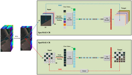
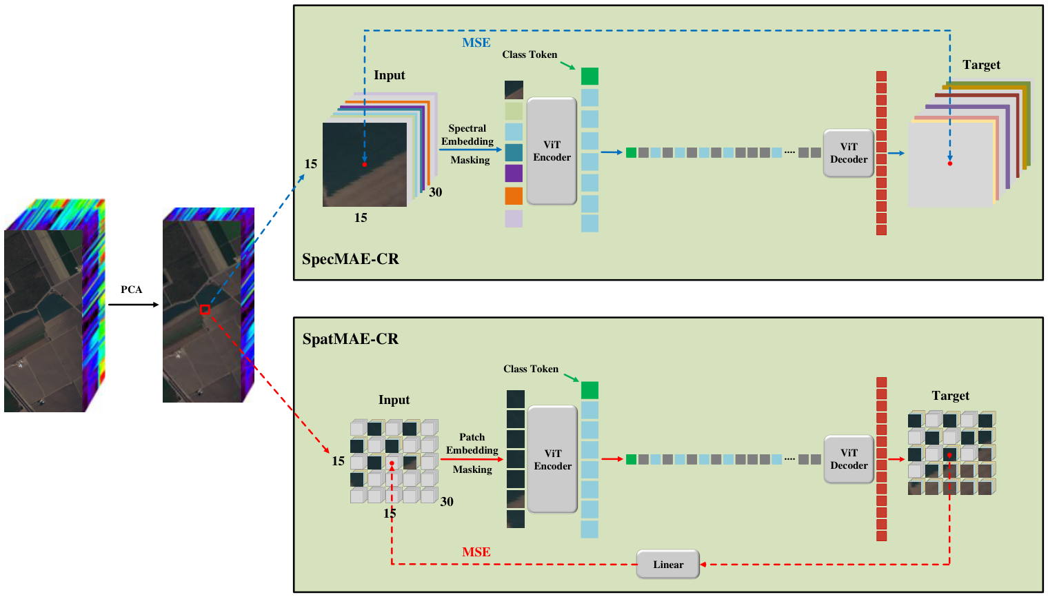
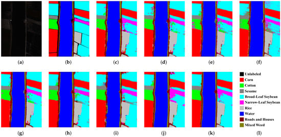
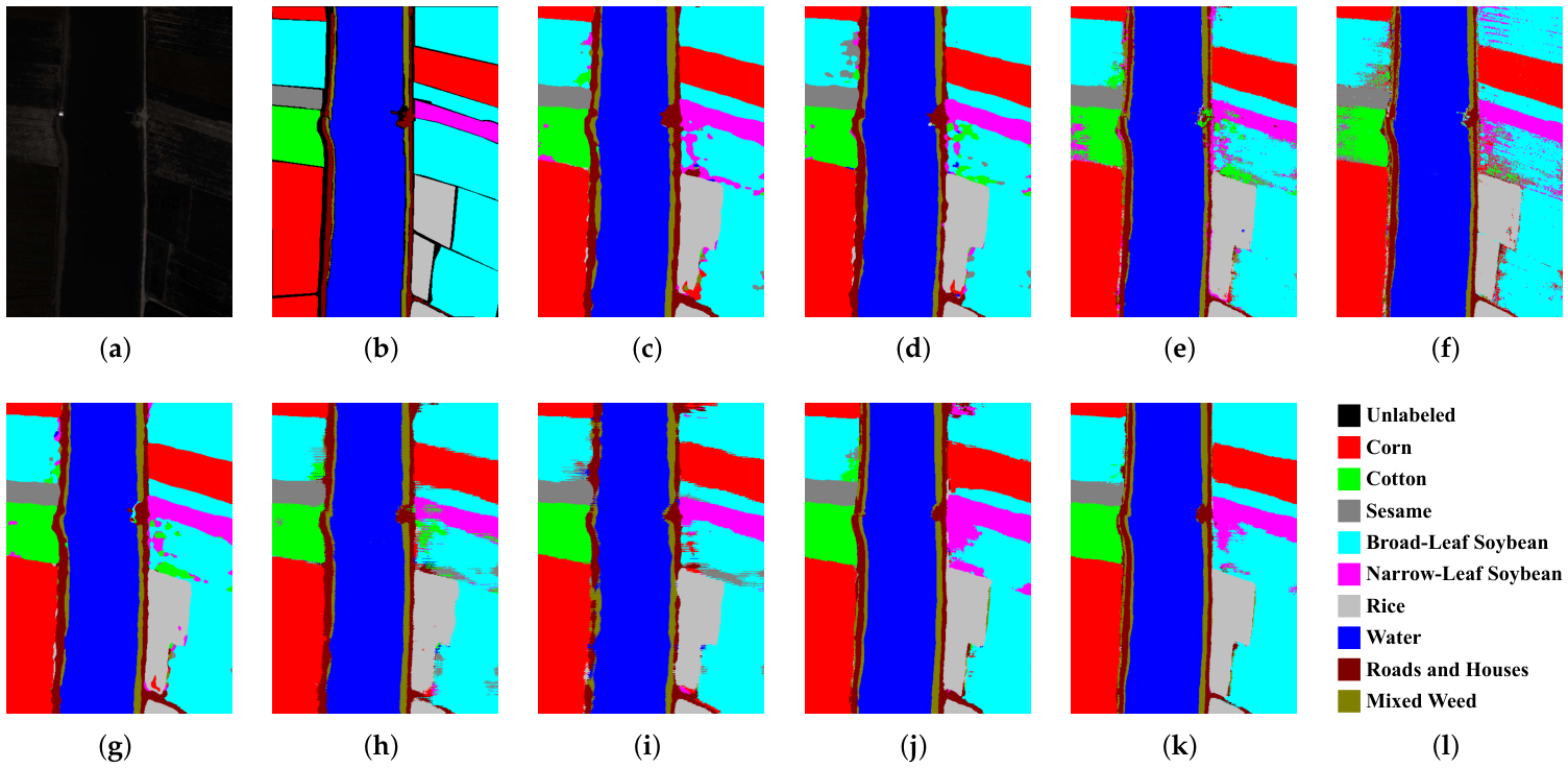
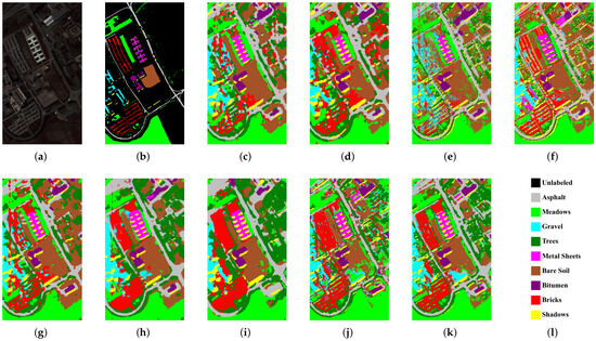
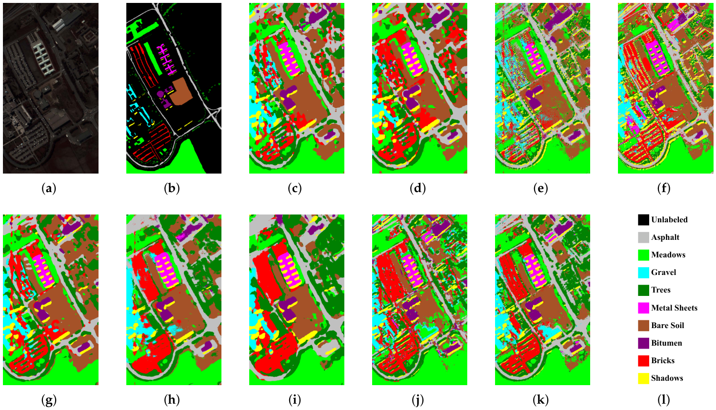
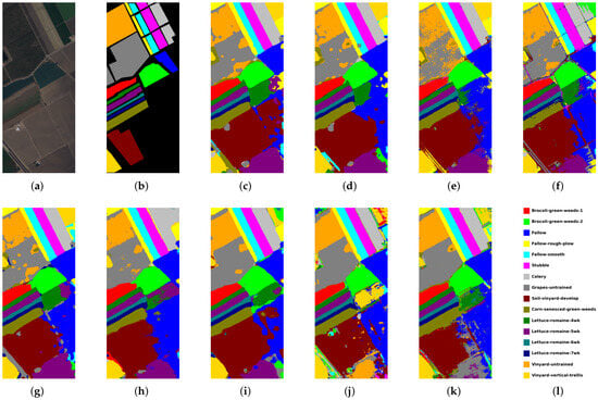
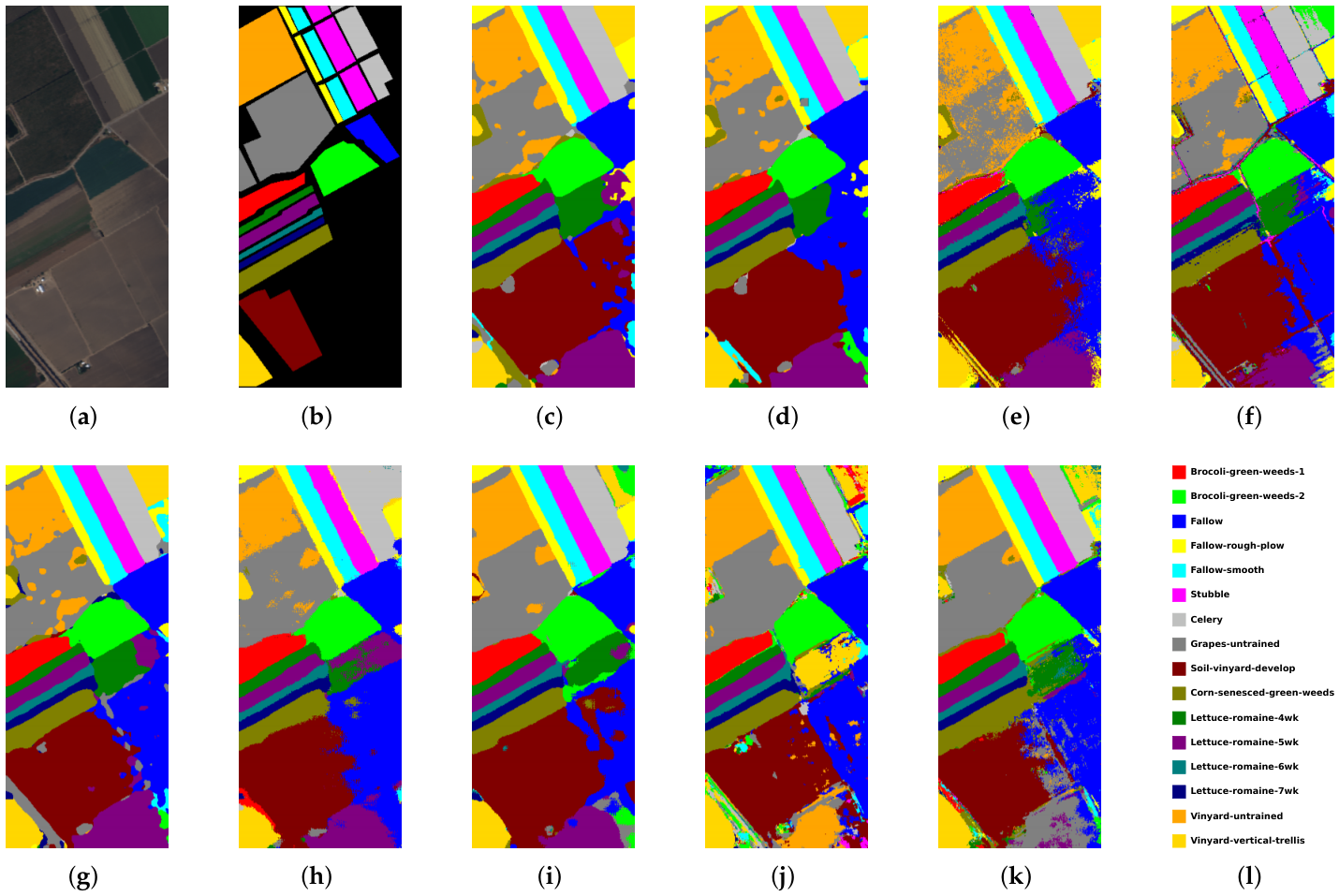
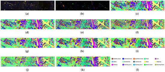
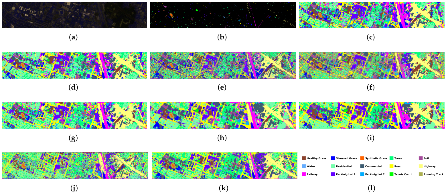
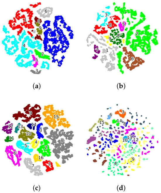
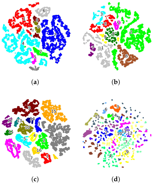
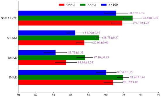
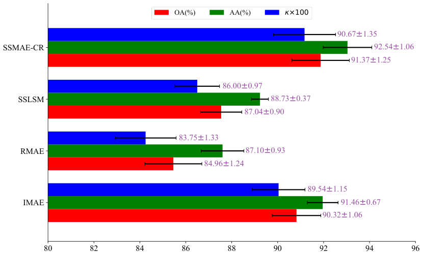
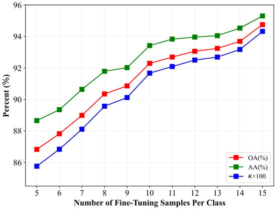
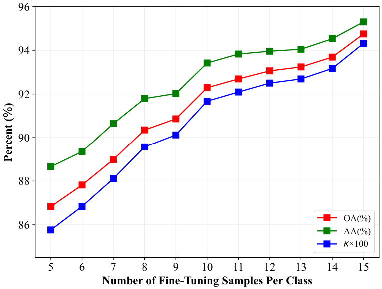
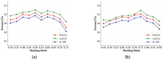
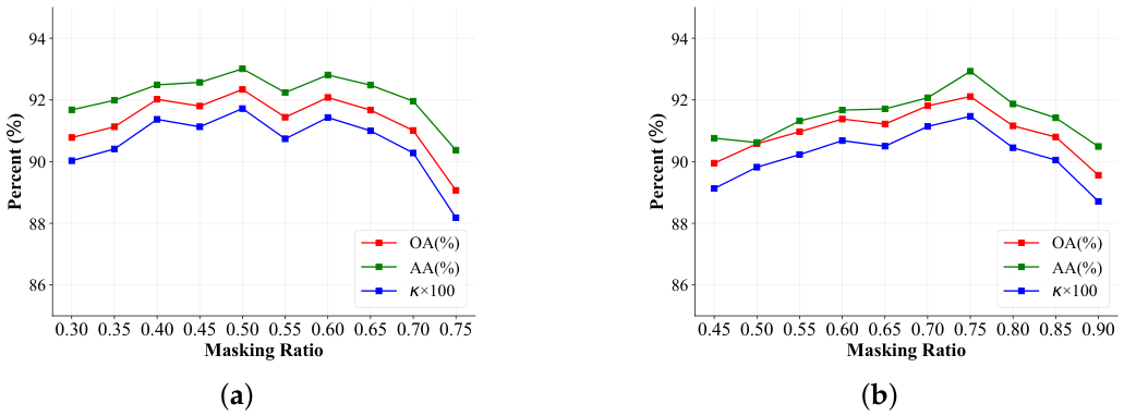

Disclaimer/Publisher’s Note: The statements, opinions and data contained in all publications are solely those of the individual author(s) and contributor(s) and not of MDPI and/or the editor(s). MDPI and/or the editor(s) disclaim responsibility for any injury to people or property resulting from any ideas, methods, instructions or products referred to in the content. |
© 2026 by the authors. Licensee MDPI, Basel, Switzerland. This article is an open access article distributed under the terms and conditions of the Creative Commons Attribution (CC BY) license.