An Image Stabilization Method for Airborne Video SAR Based on a Joint Singer-Random Walk Model

Highlights

What are the main findings?

• Conventional NCC-based registration directly uses frame-by-frame drift estimates for image stabilization, but the estimates still contain systematic bias and random errors, resulting in residual interframe jitter. This work redefines NCC-based drift estimates as drift measurements and establishes a joint state space model for long-duration airborne ViSAR image stabilization, where the true drift is represented by a two-dimensional Singer process and the systematic registration bias by a random walk process.
• Real airborne W-band ViSAR experiments show that the proposed method suppresses both interframe drift and residual jitter more effectively than direct NCC-based registration, reducing the two-dimensional drift RMSE from 3.10 to 1.31 pixels (with an error reduction rate of approximately 58%) while achieving the highest difference image entropy in each frame.

What are the implications of the main findings?

• The proposed method provides an effective solution for high-precision stabilization of long-duration airborne ViSAR image sequences, improving scene consistency and stability in multiframe imaging.
• By explicitly separating true drift from slowly varying systematic bias in NCC-based measurements, this work offers a practical state space estimation framework for enhancing the reliability of subsequent ViSAR applications such as scene surveillance, moving target discrimination, and target tracking.

Abstract

Video synthetic aperture radar (ViSAR) provides continuous multiframe images while maintaining high resolution and has become an important tool for complex scene surveillance and moving target tracking. ViSAR imaging is susceptible to interframe drift caused by motion errors, which severely degrades video stability. When registering long time series of real airborne video SAR images, conventional image registration based on Normalized Cross-Correlation (NCC) is affected by several factors, including platform residual motion errors, approximations in the imaging geometry, interpolation resampling, and SAR speckle noise. As a result, noticeable interframe jitter persists in the registered sequence, and the stabilization accuracy is insufficient to meet high-precision image stabilization requirements. To address these issues, this paper proposes an image stabilization method for airborne video SAR based on a joint Singer-random walk model. Firstly, with the first frame selected as the reference, subpixel drift measurements in the azimuth and range directions are extracted from continuous frames via NCC-based registration. Subsequently, the true drift is modeled as a two-dimensional Singer process and the systematic bias as a random walk process, yielding a joint state space model that comprises displacement, velocity, acceleration, and bias components. On this basis, a Kalman filter and a Rauch–Tung–Striebel (RTS) fixed-interval smoother are applied to perform temporal filtering and trajectory smoothing on the drift measurements, thereby producing smooth two-dimensional drift estimates that closely approximate the actual drift trajectory. Finally, the smoothed drift trajectory is used to perform frame-by-frame subpixel drift correction on the original image sequence, achieving high-precision interframe stabilization of the ViSAR imagery. The results of real data processing demonstrate that the proposed method can effectively improve the consistency and scene stability of ViSAR multi-frame imaging.

1. Introduction

Synthetic aperture radar (SAR) provides all-weather, day-and-night imaging capability and is not constrained by illumination or weather conditions. It can achieve two-dimensional high-resolution imaging of complex scenes and targets. However, conventional SAR typically requires a long synthetic aperture time, resulting in an imaging frame rate much lower than that of infrared or optical systems [1], which makes it difficult to capture dynamic scene changes [2,3]. Video Synthetic Aperture Radar (ViSAR) combines video display technology with SAR imaging technology [4,5]. Compared with conventional SAR, ViSAR can generate image sequences at a higher frame rate while maintaining high resolution, with a typical imaging frame rate of no less than 5 Hz. Based on the above advantages, ViSAR is currently widely used in the field of moving target detection and tracking [6,7].

During real data acquisition, ViSAR is susceptible to motion errors caused by factors such as atmospheric turbulence, platform vibration, and flight attitude variations. The interframe motion error phase can induce drift in multiframe images, causing the positions of stationary targets to change between consecutive frames, thereby interfering with background/moving-target discrimination and degrading the accuracy of moving-target tracking and recognition [8].

Interframe image stabilization is a critical step in ViSAR systems, and substantial research efforts have been devoted to this problem. However, for long-duration ViSAR image sequences, the image stabilization accuracy of existing methods requires further improvement. References [9,10] employ the scale-invariant feature transform (SIFT) algorithm to achieve geometric alignment of two images by matching corresponding feature points. Although this method exhibits good adaptability to translation, rotation, and scale changes, feature mismatches in nonuniform scenes may introduce image distortion during registration. For long-duration image sequences, SIFT relies on refined image feature extraction and matching [11]. Since interframe stabilization in ViSAR requires frame-by-frame registration, the overall computational burden is substantial. References [12,13,14] adopt image registration methods based on normalized cross-correlation (NCC), where the cross-correlation coefficient is used as the similarity metric. By searching for the optimal shift that maximizes the correlation coefficient, translational alignment of the image to be registered with respect to the reference image is achieved. Unlike SIFT-based methods, NCC-based registration estimates the global shift in the whole image on a unified pixel grid and does not involve local affine or nonlinear geometric transformation, thereby avoiding image distortion in nonuniform scenes. In addition, this algorithm has a simple calculation process and a relatively low computational load in long-duration sequence registration. Therefore, based on the NCC registration method, this paper conducts research on the high-precision stabilization of long-duration ViSAR image sequences.

However, in the practical application of spotlight mode airborne video SAR, relying solely on frame-by-frame NCC registration is difficult to satisfy the requirements for high-precision image stabilization. From the perspective of the imaging mechanism, the residual motion error of the platform introduces a defocus effect in the image domain. The local geometric mismatch caused by defocus and imaging geometry approximation breaks the assumption in NCC registration that the same scatterer remains invariant across frames and exhibits only positional shift, thereby causing the cross-correlation main peak position to deviate from the true value of drift. From the perspective of algorithm implementation, subpixel shift is realized through interpolation-based resampling. The interpolation-kernel type and its parameter settings alter the local gray-level fitting method, which in turn changes the peak location of the cross-correlation surface, thus introducing additional systematic bias. Moreover, SAR speckle noise induces random disturbances in the cross-correlation main-peak location, resulting in noticeable fluctuations in the frame-by-frame estimation results around the true value. The above factors cause NCC-based drift estimation to contain both slowly varying systematic bias and random errors. As a result, stationary point targets still exhibit interframe jitter in long-duration ViSAR sequences registered by this method. In this paper, interframe jitter refers to the residual reciprocating positional deviation of stationary point targets between adjacent frames after NCC-based registration. It differs from the drift discussed above, which is caused by motion errors in the echoes and manifests as a positional shift that accumulates with frame number, whereas interframe jitter arises from measurement errors in NCC-based registration and manifests as pixel-level fluctuations of the registered target position around the actual position.

The Singer model is a global statistical model whose parameters can adequately characterize the statistical properties of target motion [15,16]. By modeling acceleration as an independent state, it provides a unified framework that accommodates both maneuvering and nonmaneuvering motion models and has been widely applied to maneuvering target tracking [17]. Analysis of measured ViSAR data indicates that the azimuth and range direction drift trajectories extracted from long time series via NCC registration generally exhibit smooth, slowly varying trends superimposed with random disturbances. These trajectories show random-acceleration characteristics with a finite time constant, and the drift amount accumulates progressively with the frame number. These characteristics are approximately consistent with the Singer model assumption that acceleration follows a zero-mean first-order Markov process with exponentially decaying autocorrelation.

Based on the above analysis, this study introduces the Singer model into the stabilization of long-duration ViSAR image sequences. A two-dimensional Singer motion model is employed to represent the true drift, and an airborne ViSAR image stabilization method based on a joint Singer-random walk model is proposed. Given that systematic bias is present in the drift trajectories, the bias term is modeled as a random walk process to distinguish it from the true drift. Based on this formulation, a joint state space model is then constructed. Furthermore, a Kalman filter and a Rauch–Tung–Striebel (RTS) fixed interval smoother are employed to perform filtering and smoothing-based reconstruction of the drift trajectories over the entire frame sequence. Finally, the smoothed trajectories are used for frame-by-frame drift correction of the original image sequence.

2. NCC-Based Registration and Joint Singer-Random Walk Bias Model

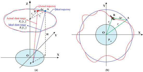
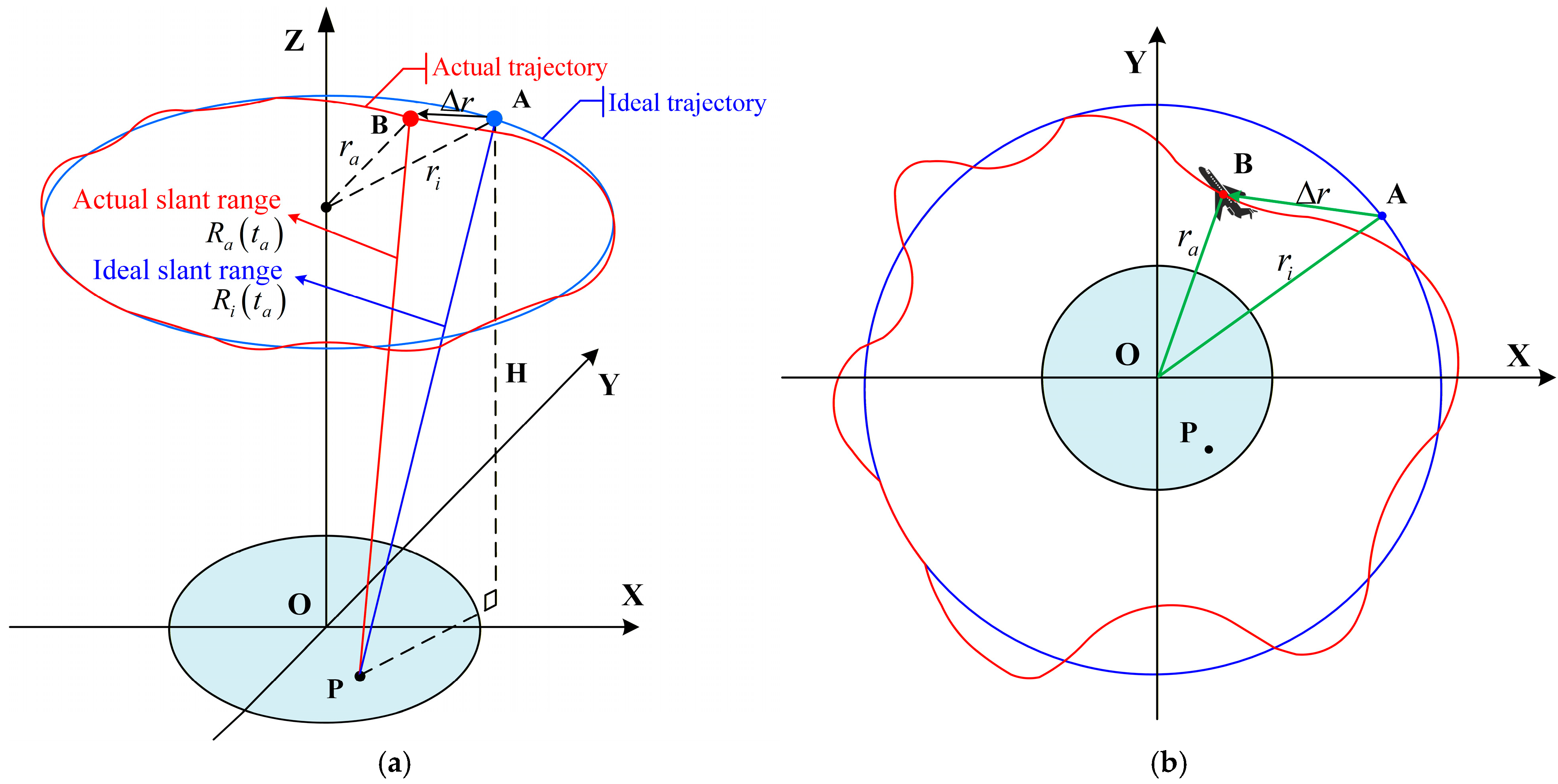
In long time series of video SAR images, even if stationary point targets remain fixed in the observed scene, their imaging positions in different frames still exhibit two-dimensional drift along the azimuth and range directions. The essential reason for this issue is the estimation errors in the platform position and velocity during real data acquisition, which cause the actual slant range $R_a$ between the antenna phase center (APC) and the point target to deviate from the ideal slant range $R_i$ assumed in the imaging model, thereby introducing motion errors into the echo signals [18]. The corresponding geometric model of airborne video SAR in spotlight mode is illustrated in Figure 1. Conventional data-driven motion compensation approaches cannot completely eliminate such errors [19,20]. The residual components exist in the form of interframe phase errors, which are converted into two-dimensional pixel drift after focusing. This drift accumulates as the frame number increases.

Figure 1. Spotlight mode airborne video SAR geometry with motion errors. (a) Geometric model; (b) Top view model.

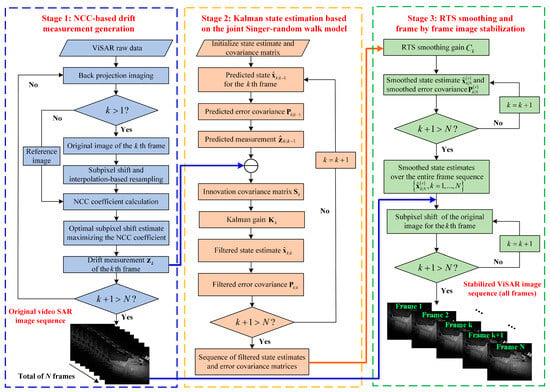
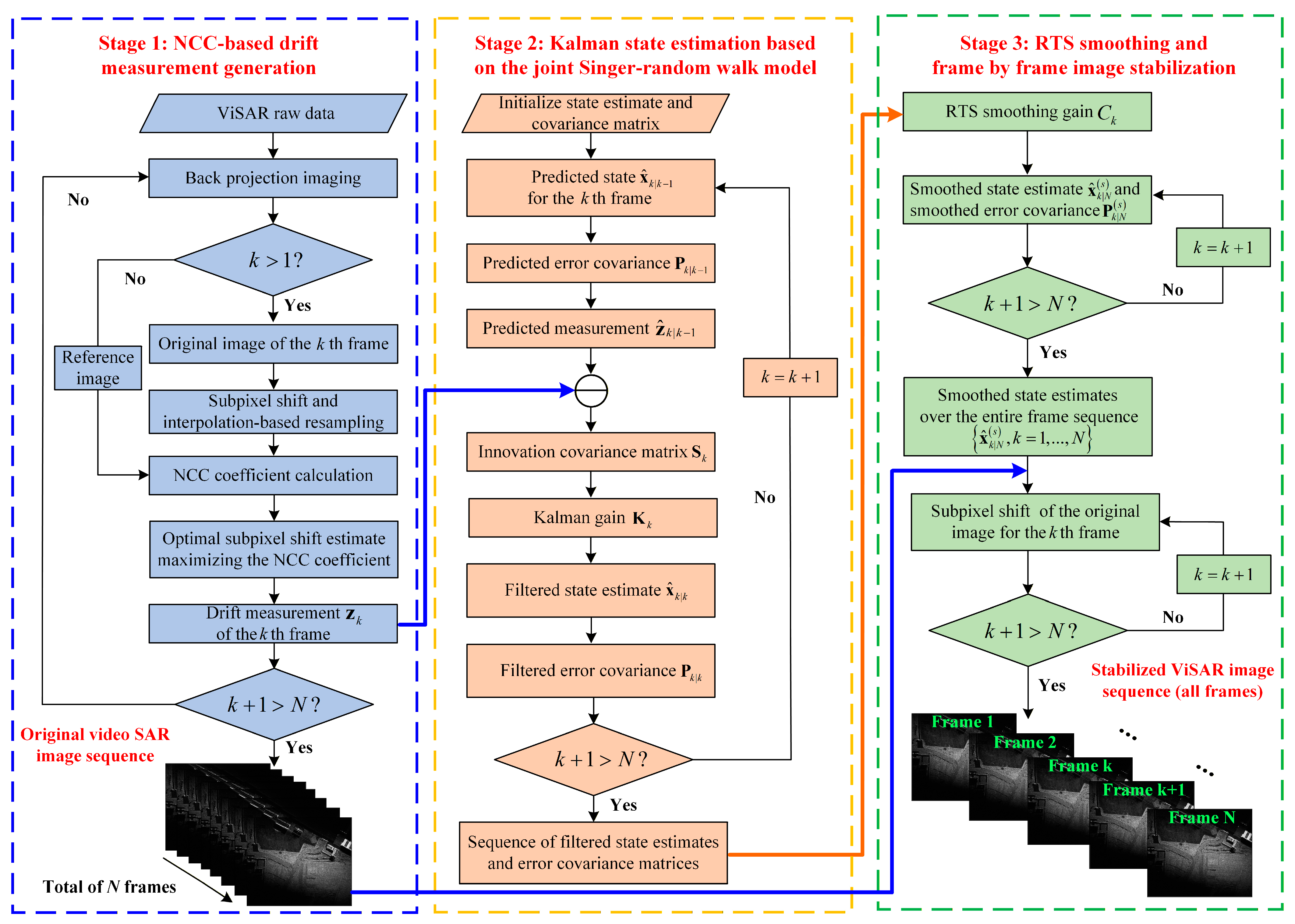
To address the above image drift, this paper proposes an image stabilization method for long-duration ViSAR image sequences. The overall processing flow is illustrated in Figure 2 and consists of three sequential stages: NCC-based drift measurement generation, Kalman filtering based on the joint Singer-random walk model, and RTS smoothing followed by frame-by-frame image stabilization.

Figure 2. Flowchart of the proposed image stabilization algorithm.

In Stage 1, the multiframe ViSAR raw data are taken as input. Frame-by-frame imaging is first performed to generate the original ViSAR images, and NCC-based registration is then applied to extract the corresponding drift measurement for each frame. Since Kalman filtering is performed sequentially, the NCC-based drift measurement of each frame can be directly used for state estimation in the next stage once it becomes available.

In Stage 2, the NCC-based drift measurements obtained in Stage 1 are taken as the input. Based on the established Singer-random walk joint state space model, a Kalman filter is employed to generate the filtered state estimate sequence and the corresponding error covariance matrices. It should be noted that these filtered state estimates are not directly used for drift correction to generate the stabilized image sequence but are instead provided as inputs to the subsequent RTS smoothing stage.

In Stage 3, after the complete filtered state sequence is obtained, the filtered state estimates and error covariance matrices from Stage 2, as well as the original ViSAR image sequence from Stage 1, are used as inputs for subsequent processing. An RTS fixed-interval smoother is applied to perform backward smoothing of the filtered state sequence, yielding the smoothed state estimate sequence. On this basis, frame-by-frame subpixel drift correction is performed on the original images using the smoothed drift estimates, thereby producing a continuous and stabilized ViSAR image sequence.

2.1. NCC-Based Subpixel Registration and Measurement Generation

Since the subsequent state space model takes the NCC-based shift estimates as drift measurements, the subpixel shift estimation procedure is described as follows.

For the ViSAR image sequence, the first frame is taken as the reference frame, and its grayscale image is denoted as $I_1$. The image to be registered at the $k$th frame is denoted as $I_k$. For a given candidate shift $\left(\Delta x,\Delta y\right)$, to avoid the influence of zero-padded regions on the correlation calculation, the normalized cross-correlation coefficient is computed only over the valid overlapping region $\Omega \left(\Delta x,\Delta y\right)$ of the two images. Accordingly, the NCC coefficient of the $k$th frame with respect to the reference frame under the candidate shift $\left(\Delta x,\Delta y\right)$ is defined as:

$${\rho }_k\left(\Delta x,\Delta y\right)={\displaystyle \frac{{\displaystyle \sum _{\left(i,j\right)\in \Omega \left(\Delta x,\Delta y\right)}\left(I_1\left(i,j\right)-{\overline{I}}_1\right)\left(I_k\left(i+\Delta x,j+\Delta y\right)-{\overline{I}}_k\right)}}{\sqrt{{\displaystyle \sum _{\left(i,j\right)\in \Omega \left(\Delta x,\Delta y\right)}{\left(I_1\left(i,j\right)-{\overline{I}}_1\right)}^2}}\sqrt{{\displaystyle \sum _{\left(i,j\right)\in \Omega \left(\Delta x,\Delta y\right)}{\left(I_k\left(i+\Delta x,j+\Delta y\right)-{\overline{I}}_k\right)}^2}}}}$$

(1)

where $i$ and $j$ denote the pixel indices in the azimuth and range directions, $I_1\left(i,j\right)$ and $I_k\left(i+\Delta x,j+\Delta y\right)$ denote the gray values of $I_1$ and $I_k$ at the corresponding pixel coordinates, respectively. ${\overline{I}}_1$ and ${\overline{I}}_k$ denote the mean gray values of the reference image and the shifted image to be registered over the valid overlapping region.

First, a coarse search is performed over the predefined integer pixel search set $S_c$, thereby obtaining the optimal integer pixel shift estimate of the $k$th frame with respect to the reference frame:

$$\left(\Delta {\widehat{x}}_k,\Delta {\widehat{y}}_k\right)=\underset{\left(\Delta x,\Delta y\right)\in S_c}{\arg \max }{\rho }_k\left(\Delta x,\Delta y\right)$$

(2)

where $\Delta {\widehat{x}}_k$ and $\Delta {\widehat{y}}_k$ denote the integer pixel shift estimates in the azimuth and range directions at the $k$th frame, respectively.

After obtaining the optimal integer pixel shift, a finer real-valued search set $S_f$ is constructed around $\left(\Delta {\widehat{x}}_k,\Delta {\widehat{y}}_k\right)$ to further improve the shift estimation accuracy. Subsequently, a subpixel-level fine search is performed over this set. Since the coordinate locations corresponding to the subpixel shifted image generally no longer coincide with the original integer pixel grid, interpolation-based resampling is required to construct the shifted image. Let ${\tilde{I}}_k^{\left(\Delta {\tilde{x}}_k,\Delta {\tilde{y}}_k\right)}\left(i,j\right)$ denote the resampled image of the $k$th frame under the subpixel candidate shift $\left(\Delta {\tilde{x}}_k,\Delta {\tilde{y}}_k\right)$, which can be expressed as:

$$\begin{array}{l}{N}_x\left(i,\Delta {\tilde{x}}_k\right)=\left\{\left.m\right|\varphi \left(i+\Delta {\tilde{x}}_k-m\right)\ne 0\right\},N_y\left(j,\Delta {\tilde{y}}_k\right)=\left\{\left.n\right|\varphi \left(j+\Delta {\tilde{y}}_k-n\right)\ne 0\right\}\\ {\tilde{I}}_k^{\left(\Delta {\tilde{x}}_k,\Delta {\tilde{y}}_k\right)}\left(i,j\right)={\displaystyle \sum _{m\in N_x}{\displaystyle \sum _{n\in N_y}{I}_k\left(m,n\right)}}\cdot \varphi \left(i+\Delta {\tilde{x}}_k-m\right)\cdot \varphi \left(j+\Delta {\tilde{y}}_k-n\right)\end{array}$$

(3)

where $N_x\left(i,\Delta {\tilde{x}}_k\right)$ and $N_y\left(j,\Delta {\tilde{y}}_k\right)$ denote the sets of integer neighborhood indices in the azimuth and range directions determined by the nonzero support of the interpolation kernel, and $\varphi \left(\cdot \right)$ denotes the one-dimensional interpolation kernel. Here, $m$ and $n$ denote the integer indices within the neighborhood of the original image to be registered in the azimuth and range directions, $I_k\left(m,n\right)$ represents the gray value at the integer pixel location $\left(m,n\right)$, and $\varphi \left(i+\Delta {\tilde{x}}_k-m\right)$ and $\varphi \left(j+\Delta {\tilde{y}}_k-n\right)$ denote the interpolation weights of the neighborhood pixel in the azimuth and range directions. As shown in Equation (3), subpixel shifting can be equivalently regarded as an interpolation-based reconstruction process of the original image to be registered. The selection of interpolation kernel alters the local gray-level reconstruction, thereby introducing systematic bias into the shift estimation.

In the fine search stage, the NCC coefficient between the resampled image and the reference image is calculated according to Equation (1). This coefficient is further maximized within the subpixel search set $S_f$, so as to obtain the optimal subpixel shift estimate of the $k$th frame:

$$\left(d_{x,k}^{obs},d_{y,k}^{obs}\right)=\underset{\left(\Delta {\tilde{x}}_k,\Delta {\tilde{y}}_k\right)\in S_f}{\arg \max }{\rho }_k\left(\Delta {\tilde{x}}_k,\Delta {\tilde{y}}_k\right)$$

(4)

where $d_{x,k}^{obs}$ and $d_{y,k}^{obs}$ denote the subpixel shift estimates in the azimuth and range directions at the $k$th frame, respectively. These estimates are taken as the drift measurements in the subsequent state space modeling.

However, the above NCC-based subpixel shift estimates are exactly equal to the true drift only under ideal conditions. In practice, NCC-based registration is affected by several factors, including local geometric mismatch from defocus and imaging geometry approximation, systematic bias introduced by interpolation-based resampling during subpixel shifting, and correlation-peak fluctuation due to SAR speckle noise. Therefore, if $\left(d_{x,k}^{obs},d_{y,k}^{obs}\right)$ is directly used for image stabilization, since the obtained drift estimation still contains non-negligible systematic bias and random errors, it will lead to interframe jitter in the registered image sequence. To uniformly model and estimate these errors, this study employs the Singer model to characterize the true drift trajectories and a random walk model to represent the systematic bias, thereby establishing a two-dimensional joint state equation.

2.2. Discrete-Time One-Dimensional Singer Motion Equation

Consider the true drift component along a given direction. Its continuous-time one-dimensional Singer motion state vector is defined as $x_s\left(t\right)={[d\left(t\right),v\left(t\right),a\left(t\right)]}^T$. Here, $d\left(t\right)$, $v\left(t\right)$, and $a\left(t\right)$ represent the drift displacement, drift velocity, and drift acceleration in continuous time, respectively. In the Singer model, the acceleration is modeled as a first-order Markov process [17], and the corresponding continuous-time state equation can be written as:

$${\dot{x}}_s\left(t\right)=A_s{x}_s\left(t\right)+G_s{w}_a\left(t\right),A_s=\left[\begin{array}{ccc}0& 1& 0\\ 0& 0& 1\\ 0& 0& -\lambda \end{array}\right],G_s=\left[\begin{array}{c}0\\ 0\\ 1\end{array}\right]$$

(5)

where $A_s$ is the continuous-time system matrix of the Singer model, $G_s$ is the continuous-time noise-gain matrix of the Singer model. $\lambda$ denotes the exponential decay rate of the acceleration autoregression and $w_a\left(t\right)$ is the zero-mean Gaussian white noise driving the acceleration stochastic process. When the continuous-time acceleration stochastic process $a\left(t\right)$ reaches the steady state, its steady-state variance is defined as ${\sigma }_a^2$. Accordingly, the relationship between the white-noise intensity of $w_a\left(t\right)$ and ${\sigma }_a^2$ is given by $\mathbb{E}\left[w_a\left(t_1\right)\cdot w_a\left(t_2\right)\right]=2\lambda {\sigma }_a^2\delta \left(t_1-t_2\right)$, where $\mathbb{E}\left[\cdot \right]$ denotes the mathematical expectation and $\delta \left(\cdot \right)$ denotes the Dirac delta function.

Let the interframe interval of the video SAR be $T_f$. The azimuth time of the $k$th frame is given by $t_k=k{T}_f$. By discretizing Equation (5) on the sampling interval $T_f$ and defining $x_{s,k}=x_s\left(t_k\right)==\left[d_k,v_k,a_k\right]$ as the one-dimensional Singer state vector at $k$th frame. Here, $d_k$, $v_k$, and $a_k$ denote the drift displacement, drift velocity, and drift acceleration at the $k$th frame, respectively. The corresponding discrete-time state equation can be obtained as:

$$\begin{array}{c}{x}_{s,k+1}=F_s{x}_{s,k}+{\eta }_{s,k}=e^{A_s{T}_f}{x}_{s,k}+{\displaystyle {\int }_{t_k}^{t_{k+1}}{e}^{A_s\left(t_{k+1}-\tau \right)}}{G}_s{w}_a\left(\tau \right)d\tau \\ F_s=\left[\begin{array}{ccc}1& T_f& {\displaystyle \frac{T_f}{\lambda }}-{\displaystyle \frac{1-e^{-\lambda T_f}}{{\lambda }^2}}\\ 0& 1& {\displaystyle \frac{1-e^{-\lambda T_f}}{\lambda }}\\ 0& 0& e^{-\lambda T_f}\end{array}\right],{\eta }_{s,k}~\mathcal{N}\left(0,Q_s\right)\end{array}$$

(6)

where $F_s$ is the discrete-time state transition matrix of the one-dimensional Singer model. ${\eta }_{s,k}=\left[{\eta }_{d,k},{\eta }_{v,k},{\eta }_{a,k}\right]$ is the Singer process noise vector at the $k$th frame. Here, ${\eta }_{d,k}$, ${\eta }_{v,k}$, and ${\eta }_{a,k}$ denote the discrete-time process noises associated with the displacement, velocity, and acceleration components at the $k$th frame, respectively. $Q_s$ denotes the corresponding process noise covariance matrix.

Moreover, ${\eta }_{s,k}$ is assumed to be Gaussian white noise. Let $\varphi \left(\tau \right)=e^{A_s\left(t_{k+1}-\tau \right)}{G}_s$, and the covariance matrix $Q_s$ of ${\eta }_{s,k}$ can be expressed as follows:

$$\begin{array}{ll}{Q}_s& =\mathbb{E}\left[\left({\eta }_{s,k}\right)\cdot {\left({\eta }_{s,k}\right)}^T\right]={\displaystyle {\int }_{t_k}^{t_{k+1}}{\displaystyle {\int }_{t_k}^{t_{k+1}}\varphi \left({\tau }_1\right)\mathbb{E}\left[w_a\left({\tau }_1\right)\cdot w_a^T\left({\tau }_2\right)\right]{\varphi }^T\left({\tau }_2\right)d{\tau }_1}}d{\tau }_2\\ & =2\lambda {\sigma }_a^2\left[\begin{array}{ccc}\begin{array}{c}{\displaystyle \frac{{\left(T_f\right)}^3}{3{\lambda }^2}}-{\displaystyle \frac{{\left(T_f\right)}^2}{{\lambda }^3}}+{\displaystyle \frac{T_f\left(1-2e^{-\lambda T_f}\right)}{{\lambda }^4}}+{\displaystyle \frac{1-e^{-2\lambda T_f}}{2{\lambda }^5}}\end{array}& \begin{array}{c}{\displaystyle \frac{{\left(T_f\right)}^2}{2{\lambda }^2}}+{\displaystyle \frac{T_f\left(e^{-\lambda T_f}-1\right)}{{\lambda }^3}}+{\displaystyle \frac{{\left(1-e^{-\lambda T_f}\right)}^2}{2{\lambda }^4}}\end{array}& \begin{array}{c}-{\displaystyle \frac{T_f{e}^{-\lambda T_f}}{{\lambda }^2}}+{\displaystyle \frac{1-e^{-2\lambda T_f}}{2{\lambda }^3}}\end{array}\\ \begin{array}{c}{\displaystyle \frac{{\left(T_f\right)}^2}{2{\lambda }^2}}+{\displaystyle \frac{T_f\left(e^{-\lambda T_f}-1\right)}{{\lambda }^3}}+{\displaystyle \frac{{\left(1-e^{-\lambda T_f}\right)}^2}{2{\lambda }^4}}\end{array}& \begin{array}{c}{\displaystyle \frac{T_f}{{\lambda }^2}}-{\displaystyle \frac{2\left(1-e^{-\lambda T_f}\right)}{{\lambda }^3}}+{\displaystyle \frac{1-e^{-2\lambda T_f}}{2{\lambda }^3}}\end{array}& \begin{array}{c}{\displaystyle \frac{{\left(1-e^{-2\lambda T_f}\right)}^2}{2{\lambda }^2}}\end{array}\\ -{\displaystyle \frac{T_f{e}^{-\lambda T_f}}{{\lambda }^2}}+{\displaystyle \frac{1-e^{-2\lambda T_f}}{2{\lambda }^3}}& {\displaystyle \frac{{\left(1-e^{-2\lambda T_f}\right)}^2}{2{\lambda }^2}}& {\displaystyle \frac{1-e^{-2\lambda T_f}}{2\lambda }}\end{array}\right]\end{array}$$

(7)

2.3. Discrete-Time Random Walk Bias Term

To explicitly account for the slowly varying systematic bias in NCC-based registration within the state space model, we extend the Singer model in Section 2.2 by introducing a one-dimensional random walk process:

$$b_{k+1}=b_k+{\eta }_{b,k},{\eta }_{b,k}~\mathcal{N}\left(0,{\sigma }_b^2\right)$$

(8)

where $b_k$ represents the bias term of the NCC-based drift estimation in the $k$th frame (e.g., a systematic bias introduced by imaging geometry approximation or interpolation resampling). ${\eta }_{b,k}$ denotes the bias increment between adjacent frames and can be regarded as an independent and identically distributed zero-mean Gaussian variable. ${\sigma }_b^2$ is the variance of bias increment ${\eta }_{b,k}$. It should be noted that, although ${\sigma }_b^2$ and the aforementioned ${\sigma }_a^2$ have similar forms, they correspond to different statistical quantities at different model levels. Specifically, ${\sigma }_a^2$ denotes the steady-state variance of the Singer acceleration process $a\left(t\right)$, whereas ${\sigma }_b^2$ denotes the variance of the random walk bias increment ${\eta }_{b,k}$. Therefore, the former is a statistical quantity defined on a continuous-time state process, whereas the latter is a statistical quantity defined on a discrete-time noise increment.

2.4. Establishment of the Two-Dimensional Joint State Transition Equation

By jointly modeling the Singer substate and the random walk bias term, the one-dimensional extended state vector along the azimuth (x) direction can be written as $x_k^x$:

$$\begin{array}{l}{x}_{s,k}^x={\left[d_{x,k},v_{x,k},a_{x,k}\right]}^T\\ x_k^x={\left[x_{s,k}^x,b_{x,k}\right]}^T={\left[d_{x,k},v_{x,k},a_{x,k},b_{x,k}\right]}^T\in {ℝ}^4\end{array}$$

(9)

$x_{s,k}^x$ denotes the Singer state vector in the azimuth direction at the $k$th frame, where $d_{x,k}$, $v_{x,k}$, and $a_{x,k}$ represent the corresponding displacement, velocity, and acceleration of the drift, respectively. $b_{x,k}$ denotes the random walk bias in the azimuth direction for the $k$th frame. By rewriting Equations (6) and (8) in matrix form, the one-dimensional discrete time state-transition equation can be expressed as:

$$\begin{array}{l}{x}_{k+1}^x=F_x{x}_k^x+q_k^x,q_k^x~\mathcal{N}\left(0,Q_x\right)\\ q_k^x={[{\eta }_{s,k}^x,{\eta }_{b,k}^x]}^T,{\eta }_{s,k}^x=\left[{\eta }_{d,k}^x,{\eta }_{v,k}^x,{\eta }_{a,k}^x\right]\\ F_x=\left[\begin{array}{cc}{F}_{s,x}& 0_{3\times 1}\\ 0_{1\times 3}& 1\end{array}\right],Q_x=\left[\begin{array}{cc}{Q}_{s,x}& 0_{3\times 1}\\ 0_{1\times 3}& {\sigma }_{b,x}^2\end{array}\right]\end{array}$$

(10)

where $F_x$ denotes the extended state transition matrix in the azimuth direction, and $F_{s,x}$ denotes the discrete-time state transition matrix of the Singer submodel in the azimuth direction. $q_k^x$ denotes the extended process noise vector in the azimuth direction at the $k$th frame. Here, ${\eta }_{s,k}^x$ denotes the Singer process noise vector in the azimuth direction at the $k$th frame, where ${\eta }_{d,k}^x$, ${\eta }_{v,k}^x$, and ${\eta }_{a,k}^x$ denote the discrete-time process noises associated with the displacement, velocity, and acceleration components in the azimuth direction, respectively. Here, $Q_x$ denotes the process noise covariance matrix of the extended state equation in the azimuth direction, and $Q_{s,x}$ denotes the discrete-time process noise covariance matrix of the Singer submodel in the azimuth direction. ${\eta }_{b,k}^x$ is the bias increment in the azimuth direction at the $k$th frame. Assuming that the discrete increments ${\eta }_{s,k}^x$ and ${\eta }_{b,k}^x$ are mutually independent, the process noise $q_k^x$ also follows a zero-mean Gaussian distribution.

Similar to the derivation in the azimuth direction, the drift component of the video SAR in the range (y) direction is then considered. Under a given interframe interval $T_f$, the corresponding discrete-time state-transition equation can be written as:

$$\begin{array}{l}{x}_{s,k}^y={\left[d_{y,k},v_{y,k},a_{y,k}\right]}^T\\ x_k^y={\left[x_{s,k}^y,b_{y,k}\right]}^T={\left[d_{y,k},v_{y,k},a_{y,k},b_{y,k}\right]}^T\\ x_{k+1}^y=F_y{x}_k^y+q_k^y,q_k^y~\mathcal{N}\left(0,Q_y\right)\\ q_k^y={[{\eta }_{s,k}^y,{\eta }_{b,k}^y]}^T,{\eta }_{s,k}^y=\left[{\eta }_{d,k}^y,{\eta }_{v,k}^y,{\eta }_{a,k}^y\right]\end{array}$$

(11)

where $x_k^y$ denotes the extended state vector in the range direction at the $k$th frame. $x_{s,k}^y$ denotes the Singer state vector in the range direction at the $k$th frame, where $d_{y,k}$, $v_{y,k}$, and $a_{y,k}$ represent the corresponding displacement, velocity, and acceleration of the drift, respectively. $b_{y,k}$ denotes the random walk bias in the range direction for the $k$th frame. $F_y$ denotes the extended state transition matrix in the range direction. $q_k^y$ denotes the extended process noise vector in the range direction at the $k$th frame. Here, ${\eta }_{s,k}^y$ denotes the Singer process noise vector in the range direction at the $k$th frame, where ${\eta }_{d,k}^y$, ${\eta }_{v,k}^y$, and ${\eta }_{a,k}^y$ denote the discrete-time process noises associated with the displacement, velocity, and acceleration components in the range direction, respectively. $Q_y$ denotes the process noise covariance matrix of the extended state equation in the range direction. ${\eta }_{b,k}^y$ is the bias increment in the range direction at the $k$th frame.

By comparing Equations (10) and (11), it can be observed that the discrete-time state transition equations in the azimuth and range directions have identical forms. By assigning separate parameters to the two directions, including $\left({\lambda }_x,{\lambda }_y\right)$, $\left({\sigma }_{a,x}^2,{\sigma }_{a,y}^2\right)$, and $\left({\sigma }_{b,x}^2,{\sigma }_{b,y}^2\right)$, the variation trend and statistical differences in the image drift in long-duration sequences can be effectively reflected. Here, ${\lambda }_x$ and ${\lambda }_y$ represent the exponential decay rates of the acceleration autoregression, ${\sigma }_{a,x}^2$ and ${\sigma }_{a,y}^2$ represent the steady-state variances of the acceleration stochastic processes, and ${\sigma }_{b,x}^2$ and ${\sigma }_{b,y}^2$ represent the variances of the random walk bias increments, in the azimuth and range directions, respectively.

Furthermore, to obtain a unified state space representation of the two-dimensional drift process in video SAR images, the one-dimensional state vectors in the azimuth and range directions are stacked component-wise. The resulting joint state vector $x_k$ and joint process noise vector $q_k$ are defined as:

$$\begin{array}{l}{x}_k={\left[x_k^x,x_k^y\right]}^T={\left[d_{x,k},v_{x,k},a_{x,k},b_{x,k},d_{y,k},v_{y,k},a_{y,k},b_{y,k}\right]}^T\in {ℝ}^8\\ q_k={\left[q_k^x,q_k^y\right]}^T={\left[{\eta }_{d,k}^x,{\eta }_{v,k}^x,{\eta }_{a,k}^x,{\eta }_{b,k}^x,{\eta }_{d,k}^y,{\eta }_{v,k}^y,{\eta }_{a,k}^y,{\eta }_{b,k}^y\right]}^T\in {ℝ}^8\end{array}$$

(12)

Based on Equation (12), the one-dimensional state transition equations in the two directions can be combined into a two-dimensional joint form using a block diagonal matrix:

$$\begin{array}{l}{x}_{k+1}=F{x}_k+q_k,q_k~\mathcal{N}\left(0,Q\right)\\ F=\left[\begin{array}{cc}{F}_x& 0_{4\times 4}\\ 0_{4\times 4}& F_y\end{array}\right],Q=\left[\begin{array}{cc}{Q}_x& 0_{4\times 4}\\ 0_{4\times 4}& Q_y\end{array}\right]\end{array}$$

(13)

where $F\in {ℝ}^{8\times 8}$ denotes the two-dimensional joint state-transition matrix and $Q\in {ℝ}^{8\times 8}$ is the covariance matrix of the two-dimensional joint process noise. From Equations (12) and (13), it follows that, for each frame, the joint state vector simultaneously comprises the drift displacement, velocity, acceleration, and their associated random walk biases in both the azimuth and range directions. Through the state-transition equation, these state components collectively reflect the temporal correlation of the drift sequence.

3. Kalman Filtering and RTS Smoothing

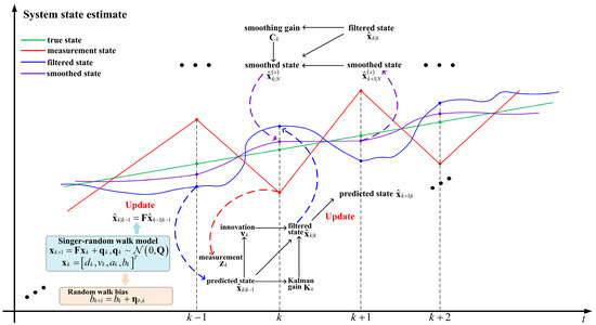
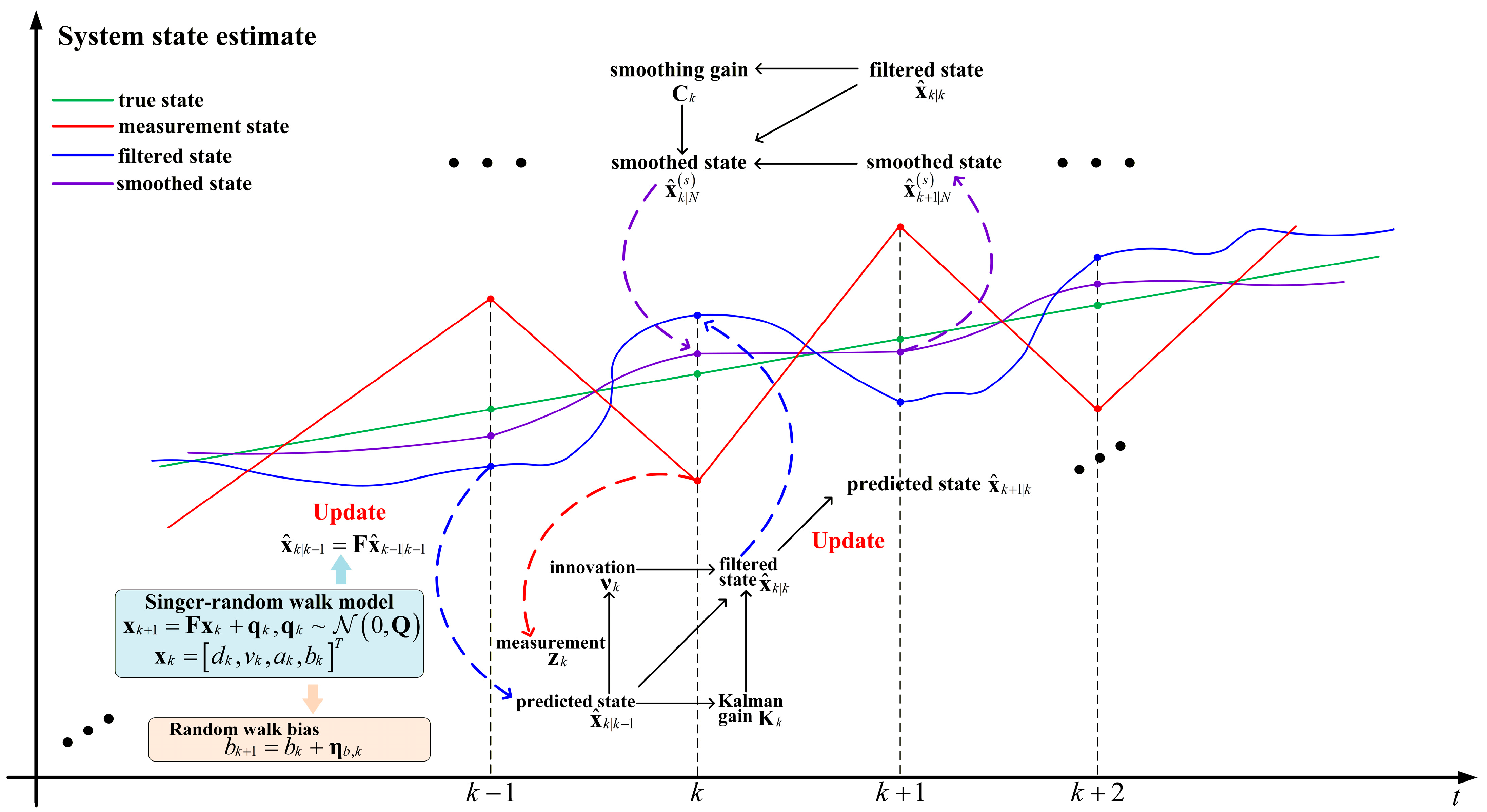
In Section 2, the state transition equation for the interframe drift of ViSAR is established based on the joint Singer-random walk bias model. In this section, the measurement equation is formulated using the drift measurements obtained from NCC registration, thereby completing the state space model used for interframe drift estimation. Sequential state estimation of the two-dimensional drift trajectories is then performed by Kalman filtering, followed by RTS fixed-interval smoothing to reconstruct these trajectories. Finally, the resulting per-frame drift correction values for ViSAR multiframe image stabilization are obtained. The procedure of Kalman filtering and RTS smoothing is illustrated in Figure 3. It should be noted that Figure 3 is only a schematic illustration used to show the recursive relationship between Kalman filtering and RTS smoothing. Although the proposed model is established as a two-dimensional joint state space model in the range and azimuth directions, the filtering and smoothing recursions in the two dimensions have the same form. Therefore, only a one-dimensional trajectory is shown in Figure 3 for clarity.

Figure 3. Schematic illustration of Kalman filtering and RTS smoothing.

3.1. Kalman Filter Model Formulation

Taking the first frame as the reference, the full image NCC registration is performed on the $k$th frame, yielding the corresponding two-dimensional drift measurement vector $z_k={[d_{x,k}^{obs},d_{y,k}^{obs}]}^T$. Under ideal conditions, $d_{x,k}^{obs}$ and $d_{y,k}^{obs}$ would be equal to the true drift components $d_{x,k}$ and $d_{y,k}$. However, as analyzed in the previous section, the practical drift measurements generally contain both systematic bias and measurement noise. Accordingly, the drift measurements obtained from NCC registration can be modeled as:

$$z_k=\left[\begin{array}{l}{d}_{x,k}^{obs}\\ d_{y,k}^{obs}\end{array}\right]=\left[\begin{array}{l}{d}_{x,k}+b_{x,k}+r_{x,k}\\ d_{y,k}+b_{y,k}+r_{y,k}\end{array}\right]$$

(14)

where $r_{x,k}$ and $r_{y,k}$ represent the measurement noise in the azimuth and range directions, respectively. By rewriting Equation (14) in matrix form, the measurement equation corresponding to the joint state vector $x_k$ can be expressed as:

$$\begin{array}{l}{z}_k=H{x}_k+r_k,r_k~\mathcal{N}\left(0,R\right)\\ H=\left[\begin{array}{cccccccc}1& 0& 0& 1& 0& 0& 0& 0\\ 0& 0& 0& 0& 1& 0& 0& 1\end{array}\right]\end{array}$$

(15)

where $H$ denotes the measurement matrix, $r_k$ is the measurement noise vector modeled as zero-mean Gaussian white noise, and $R$ is the covariance matrix of the measurement noise.

By combining the state equation in (13) with the measurement equation in (15), the interframe drift in video SAR can be modeled as a standard linear Gaussian state space model. Let ${\widehat{x}}_{k|k}$ denote the filtered state estimate of the $k$th frame obtained using the measurements up to frame $k$, and ${\widehat{x}}_{k|k-1}$ be the predicted state estimate of the $k$th frame obtained using only the measurements up to frame $k-1$. The corresponding error covariance matrices are denoted by $P_{k|k}$ and $P_{k|k-1}$, respectively. Suppose the total number of frames in the video SAR sequence is $N$, ${\widehat{x}}_{0|0}$ and $P_{0|0}$ are the initial state estimate and its covariance matrix.

Before obtaining the measurement of the $k$th frame, the predicted state estimate and its error covariance matrix are calculated according to the state transition equation:

$${\widehat{x}}_{k|k-1}=F{\widehat{x}}_{k-1|k-1},P_{k|k-1}=F{P}_{k-1|k-1}{F}^T+Q$$

(16)

After acquiring the measurement $z_k$ of the $k$th frame, the innovation ${\nu }_k$ and the innovation covariance matrix $S_k$ are constructed based on the predicted measurement ${\widehat{z}}_{k|k-1}=H{\widehat{x}}_{k|k-1}$ as follows:

$${\nu }_k=z_k-{\widehat{z}}_{k|k-1},S_k=H{P}_{k|k-1}{H}^T+R$$

(17)

where ${\nu }_k$ represents the deviation between the actual measurement and the predicted measurement, and $S_k$ is used to quantify the statistical uncertainty of the deviation.

Based on Equation (17), the Kalman gain is computed, and the filtered state estimate and its error covariance for the $k$th frame are updated as follows:

$$\begin{array}{l}{K}_k=P_{k|k-1}{H}^T{S}_k^{-1}\\ {\widehat{x}}_{k|k}={\widehat{x}}_{k|k-1}+K_k{\nu }_k\\ P_{k|k}=\left(I-K_{k}H\right)P_{k|k-1}\end{array}$$

(18)

It should be noted that, although the measurement equation directly includes only the displacement and bias terms, the velocity and acceleration states remain estimable. Owing to the state transition relationships between displacement, velocity, and acceleration established by the Singer model, the velocity and acceleration states are implicitly reflected in the displacement measurements across multiple frames. Accordingly, in Kalman filtering, the innovation of the current frame can update velocity and acceleration through the cross-covariance terms in the predicted covariance matrix, thereby enabling their recursive estimation [21,22].

According to the recursion from Equation (16) to Equation (18), the filtered state sequence $\left\{{\widehat{x}}_{k|k},k=1,2,\dots ,N\right\}$ is obtained. The components ${\widehat{d}}_x\left(k\right)$ and ${\widehat{d}}_y\left(k\right)$ provide estimates of the drift relative to the reference frame, while ${\widehat{b}}_x\left(k\right)$ and ${\widehat{b}}_y\left(k\right)$ account for the slowly varying systematic bias accumulated in the NCC-based drift measurements. In this way, the true drift and the systematic bias are explicitly separated in the state space model, which forms the basis for subsequent fixed-interval smoothing and multiframe stabilization.

3.2. Rauch–Tung–Striebel Smoothing

The ${\widehat{x}}_{k|k}$ obtained in Section 3.1 are causal state estimates, which are computed using only the first $k$ measurements $\left\{z_1,\dots ,z_k\right\}$. However, from the perspective of the entire measurement sequence $\left\{z_1,\dots ,z_N\right\}$, the subsequent measurements also contain information that can be used to refine the drift state estimates at earlier time instants. Therefore, based on the forward Kalman filtering results, the RTS fixed interval smoother [23] is introduced to perform a backward recursion on the filtered state sequence, enabling the state estimate at each frame to utilize both past and future measurements. The RTS smoothing provides the optimal noncausal state estimate in the mean square error sense, which not only more accurately approximates the true drift state but also improves the smoothness and consistency of the estimated trajectory over long time series.

The initial condition for RTS smoothing is set to ${\widehat{x}}_{N|N}^{\left(s\right)}={\widehat{x}}_{N|N}$,$P_{N|N}^{\left(s\right)}=P_{N|N}$. Subsequently, starting from the filtered state at $k=N-1$, a backward recursion is performed for $k=N-1,N-2,\dots ,1$. The smoothing gain of RTS for the $k$th frame is defined as:

$$C_k=P_{k|k}{F}^T{\left(P_{k+1|k}\right)}^{-1}$$

(19)

Given $C_k$, the smoothed state estimate at the $k$th frame and the corresponding smoothed error covariance matrix can be written as:

$$\begin{array}{l}{\widehat{x}}_{k|N}^{\left(s\right)}={\widehat{x}}_{k|k}+C_k\left({\widehat{x}}_{k+1|N}^{\left(s\right)}-{\widehat{x}}_{k+1|k}\right)\\ P_{k|N}^{\left(s\right)}=P_{k|k}+C_k\left(P_{k+1|N}^{\left(s\right)}-P_{k+1|k}\right)C_k^T\end{array}$$

(20)

After completing the backward recursion as shown in Equations (19) and (20), the smoothed state estimates $\{{\widehat{x}}_{k|N}^{\left(s\right)},P_{k|N}^{\left(s\right)},k=1,\dots ,N\}$ for the entire sequence can be obtained, where $P_{k|N}^{\left(s\right)}$ is used to quantitatively evaluate the uncertainty of the drift estimates of each frame. The state components ${\widehat{d}}_{x.k}^{\left(s\right)}$ and ${\widehat{d}}_{y.k}^{\left(s\right)}$ in ${\widehat{x}}_{k|N}^{\left(s\right)}$ correspond to the smoothed drift estimates in the azimuth and range directions of the $k$th frame, respectively. By applying a two-dimensional shift of $\left(-{\widehat{d}}_{x.k}^{\left(s\right)},-{\widehat{d}}_{y.k}^{\left(s\right)}\right)$ to the original video SAR image of the $k$th frame relative to the reference frame, interframe stabilization is achieved in the image domain. The pseudocode of the proposed image stabilization algorithm is provided in Appendix A.

4. Experimental Validation on Real Data

4.1. Comparison of Stabilization Results

To validate the effectiveness of the proposed method, this section presents the processing and analysis of raw W-band airborne video SAR data. The data are collected by a video SAR system mounted on a Cessna 208B aircraft. The radar operates in spotlight mode, and the platform flies at a velocity and altitude of approximately 69 m/s and 2.5 km, respectively. Considering that higher-order motion errors in the raw echoes can introduce additional defocus, such as elevated sidelobe levels and mainlobe broadening [24,25], the position of the cross-correlation main peak may deviate further from the true drift. This increases the errors in the drift measurements obtained by NCC-based registration and consequently degrades the accuracy of the subsequent image stabilization processing. Therefore, to obtain well-focused SAR images and provide reliable inputs for the NCC registration, the phase gradient autofocus (PGA) [26,27] algorithm is first applied to estimate and compensate for the higher-order phase errors. On this basis, the back projection (BP) algorithm is then used to generate a total of 400 frames of ViSAR imagery. All subsequent processing and analysis in this paper are conducted based on the above BP imaging results. The main parameters of the video SAR system and imaging are shown in Table 1.

Table 1. Main parameter of raw data.

Parameter	Value
Operational band	W
Signal bandwidth	900 MHz
Pulse repetition frequency	10,000 Hz
Platform velocity	69 m/s
Flight altitude	2.5 km
Image grid(range × azimuth)	0.3 m × 0.3 m
Scene size(range × azimuth)	2048 × 2048
Frame rate	5 Hz

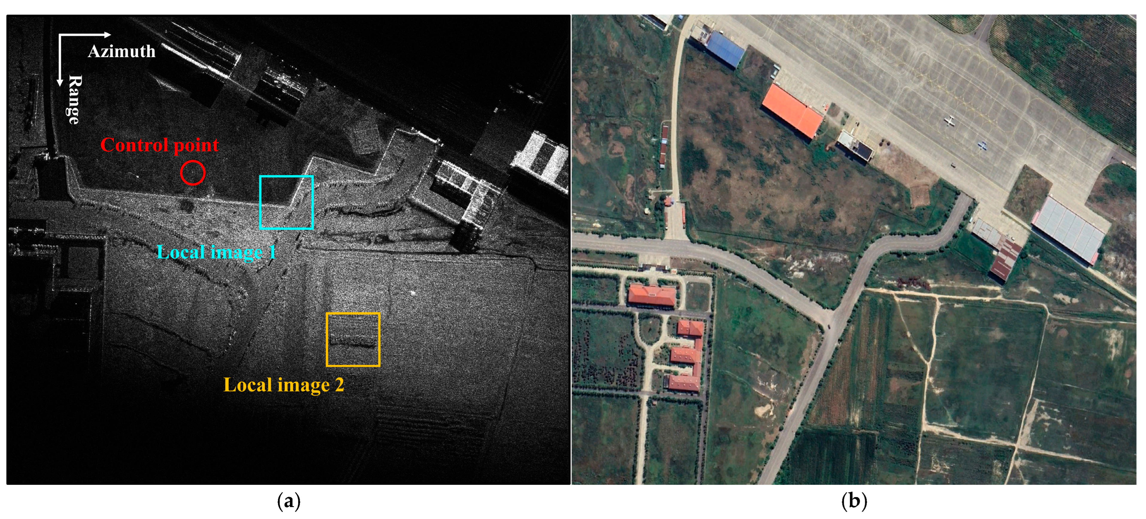
Figure 4 presents the imaging results of the observed scene. A control point is selected from the scene to obtain the true value of the drift trajectory, and two local images are extracted to quantitatively evaluate the image stabilization accuracy of different methods. Each local image has a size of 128 × 128 pixels, with a pixel spacing of 0.3 m × 0.3 m (range × azimuth).

Figure 4. Imaging result of W-band airborne ViSAR. (a) Selection of control points and local images in the scene; (b) Optical image of the scene.

It should be noted that the selected control point is used solely to provide a reference of the true value for image stabilization performance evaluation, so as to carry out quantitative comparison among different methods. Since in practical observation scenarios it is difficult to obtain an ideal calibration point with known position and strong scattering, the true drift cannot be directly derived from a single calibration point and used for frame-by-frame drift correction. Consequently, the processing based on the true drift trajectory is only employed at the algorithm verification stage and does not represent the stabilization procedure in practical applications.

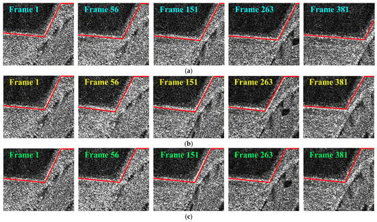
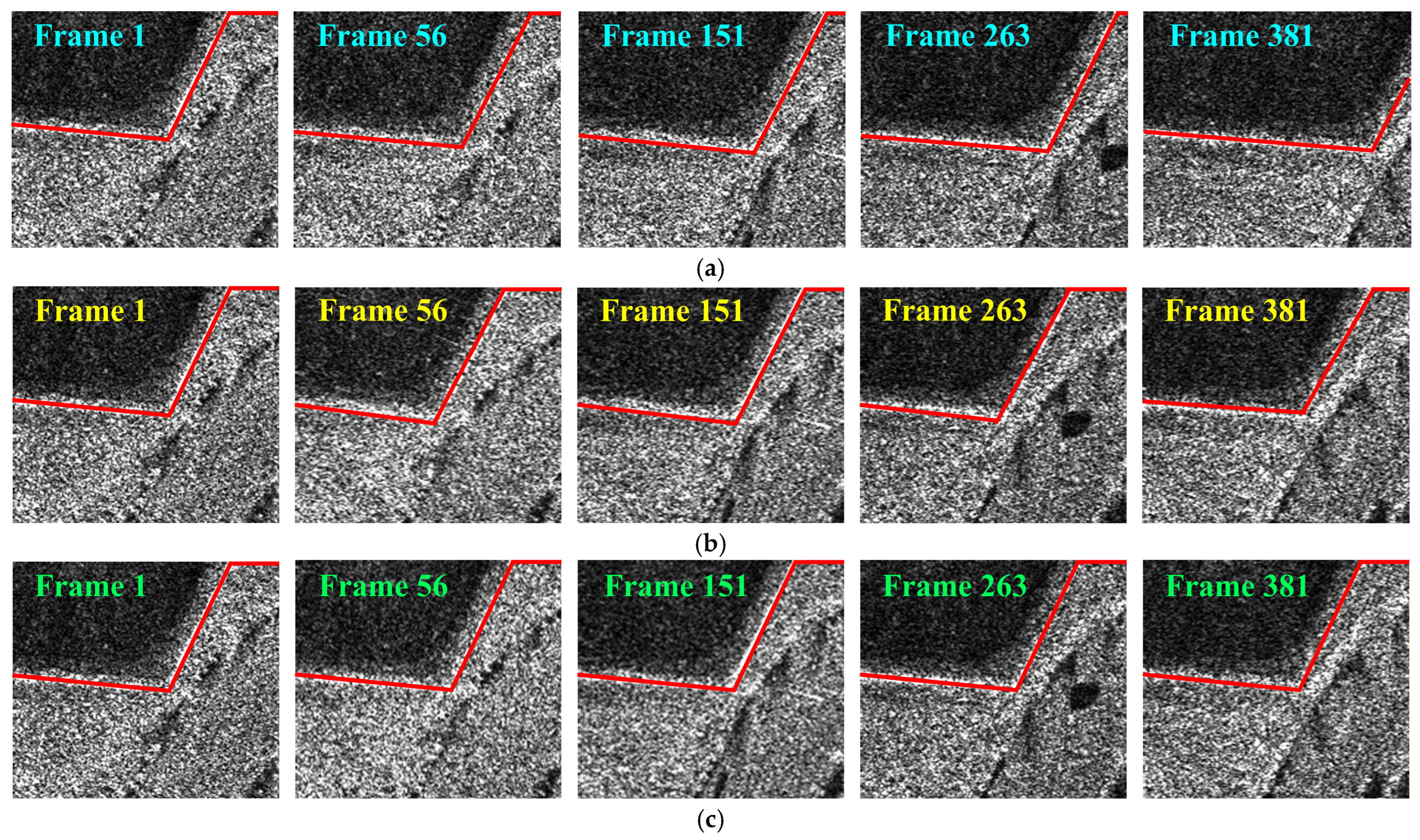
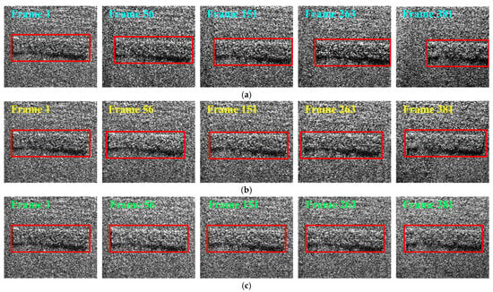
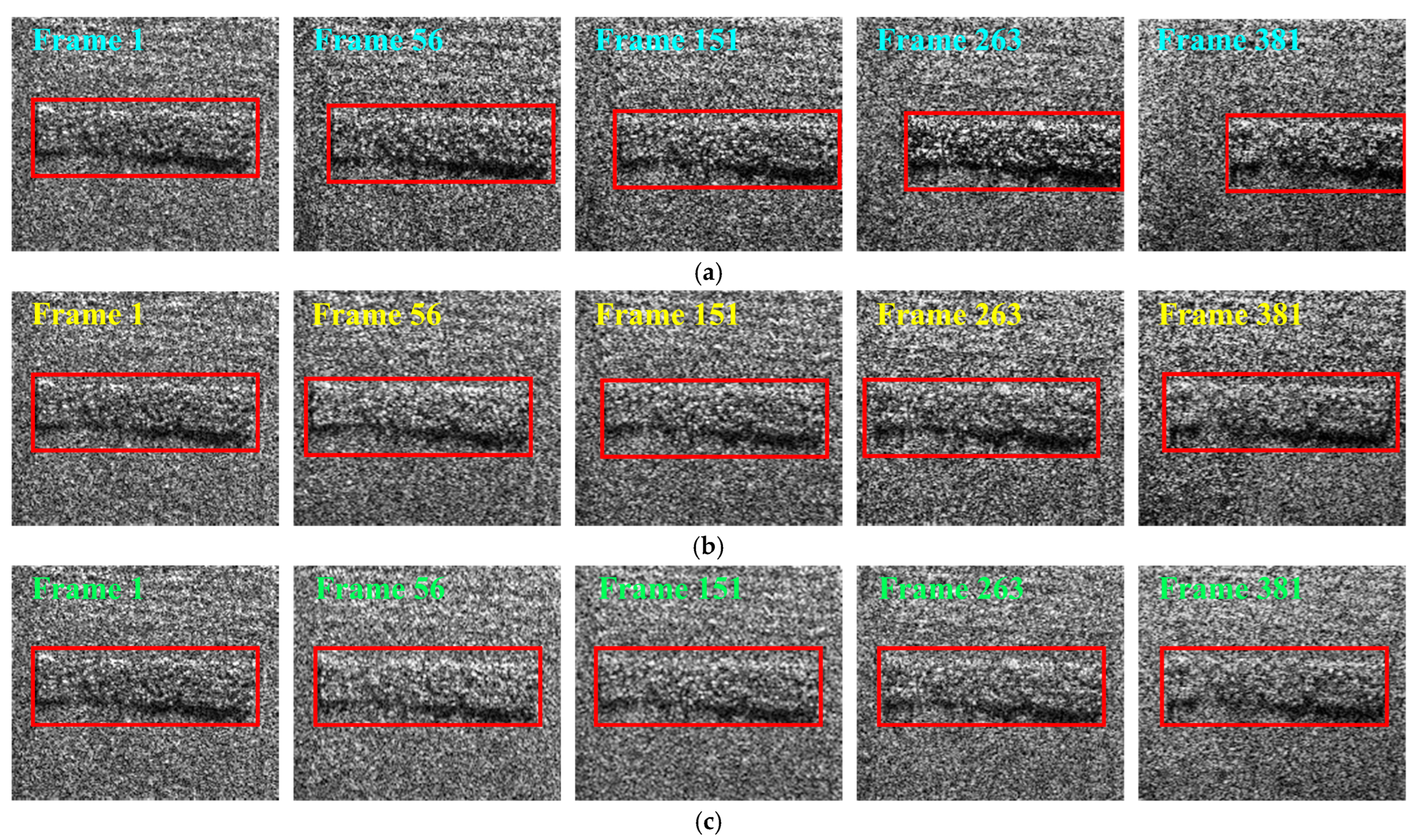
Figure 5a–c and Figure 6a–c show the stabilization results of the two subimages for frames 1, 56, 151, 263, and 381 in the original image sequence, with NCC-based registration, and with the proposed method. The average processing time of the proposed method is approximately 0.75 s per frame, including NCC-based drift measurement generation, Kalman filtering, RTS smoothing, and the final image stabilization of the corresponding original frame. To facilitate visual comparison of the stabilization performance, red polylines and rectangular boxes are used to mark local regions and highlight the detailed position changes in point targets across frames.

Figure 5. Comparison of subimage 1 for different methods. (a) Original; (b) NCC-based registration; (c) Proposed method.

Figure 6. Comparison of subimage 2 for different methods. (a) Original; (b) NCC-based registration; (c) Proposed method.

From the original sequence, it can be observed that the point target exhibits cumulative drift along both the azimuth and range directions as the frame index increases. After NCC-based registration, although the interframe drift is suppressed, there is still a small amplitude of reciprocating positional deviation between frames, i.e., interframe jitter. In contrast, after applying the proposed method, the same point target is corrected to a fixed position in the scene in every frame, and both interframe drift and jitter are effectively eliminated.

4.2. Evaluation of Stabilization Accuracy

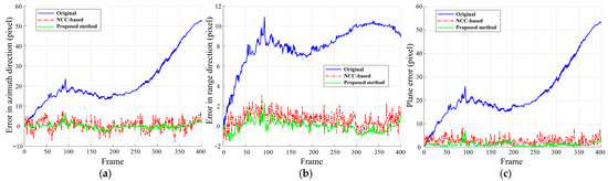
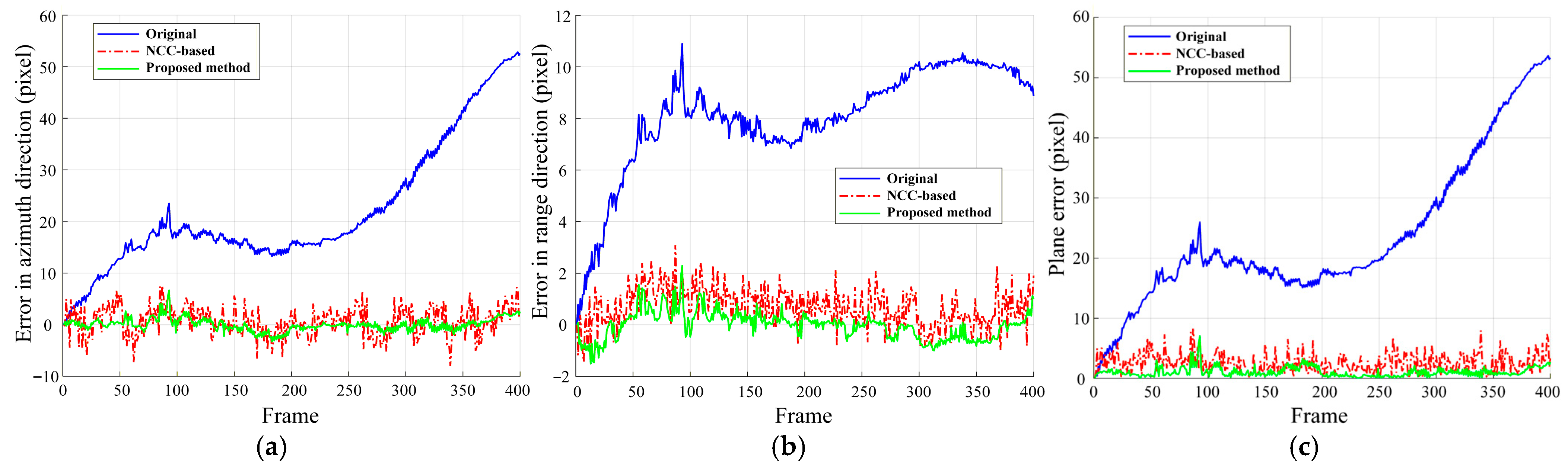
After each method is used to perform frame-by-frame stabilization of the original image sequence, the pixel coordinates of the control point in the first frame are taken as the reference position. The positional deviation of the same control point in each subsequent frame with respect to this reference position is defined as the residual error value. Figure 7 shows the residual drift error curves of subsequent frames in the azimuth and range directions as well as in the two-dimensional image plane for the different methods. The two-dimensional residual error is defined as the Euclidean distance between the azimuth and range error components. Table 2 lists the numerical residual error values of Frames 56, 151, 263, and 381 extracted from the corresponding residual error curves in Figure 7. Therefore, Table 2 and Figure 7 essentially correspond to the same set of quantitative analysis results, with Figure 7 showing the complete error variation trends and Table 2 providing representative numerical comparisons for the selected frames.

Figure 7. Residual drift error under different methods. (a) Error in azimuth direction; (b) Error in range direction; (c) Plane error.

Table 2. Residual error values of the control point for the selected frames in Figure 7.

Frame Index	Azimuth Error (Pixel)			Range Error (Pixel)
	Original Sequence	NCC-Based Registration	Proposed Method	Original Sequence	NCC-Based Registration	Proposed Method
Frame 1 (reference)	0	0	0	0	0	0
Frame 56	15.06	−4.16	−0.02	7.22	1.96	0.37
Frame 151	16.69	5.26	−0.39	7.56	1.72	0.24
Frame 263	20.55	−4.74	0.50	8.98	2.10	0.04
Frame 381	49.76	4.80	0.95	10.01	−0.51	−0.06

As shown in Figure 7 and Table 2, the two-dimensional drift error of the original sequence generally increases with the number of frames, and has reached several tens of pixels in the final frame. After NCC-based registration, the residual error fluctuates around zero and remains at the level of a few pixels per frame. In contrast, the proposed method significantly reduces both the magnitude and fluctuation of the residual error over the entire frame sequence. The residual errors in both the azimuth and range directions are effectively confined within an interval from the subpixel level to approximately one pixel.

Meanwhile, Table 3 summarizes the root mean square error (RMSE) of the drift estimates for each method over the entire frame sequence. It can be observed that the two-dimensional positional RMSE of the drift trajectory obtained with NCC-based registration is 3.10 pixels, whereas that achieved by the proposed method is reduced to 1.31 pixels. Compared with the NCC registration method, the error reduction is approximately 58%.

Table 3. RMSE statistics for different methods.

Direction	RMSE(400 Frames)
	Original Sequence	NCC-Based Registration	Proposed Method
Azimuth	25.3	2.92	1.21
Range	8.31	1.05	0.51
2-D plane	26.7	3.10	1.31

In this paper, the difference image entropy is used to quantitatively evaluate the image stabilization effect. Firstly, the reference image and the stabilized image are normalized to [0, 1] under a unified amplitude scale. Then, the corresponding difference image is obtained by pixel-wise subtraction, which reflects the influence of residual drift error on the amplitude-distribution characteristics of the image. The image entropy of the difference image can be computed using Equation (21).

$$E_p=-{\displaystyle \sum _{j=1}^{N_y}{\displaystyle \sum _{i=1}^{N_x}\left[P\left(i,j\right)\cdot \ln P\left(i,j\right)\right]}}$$

(21)

where $N_x$ and $N_y$ denote the number of pixels in azimuth and range directions, respectively. $P\left(i,j\right)$ represents the image amplitude density of the difference image at pixel $\left(i,j\right)$.

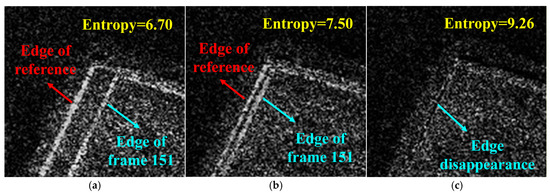
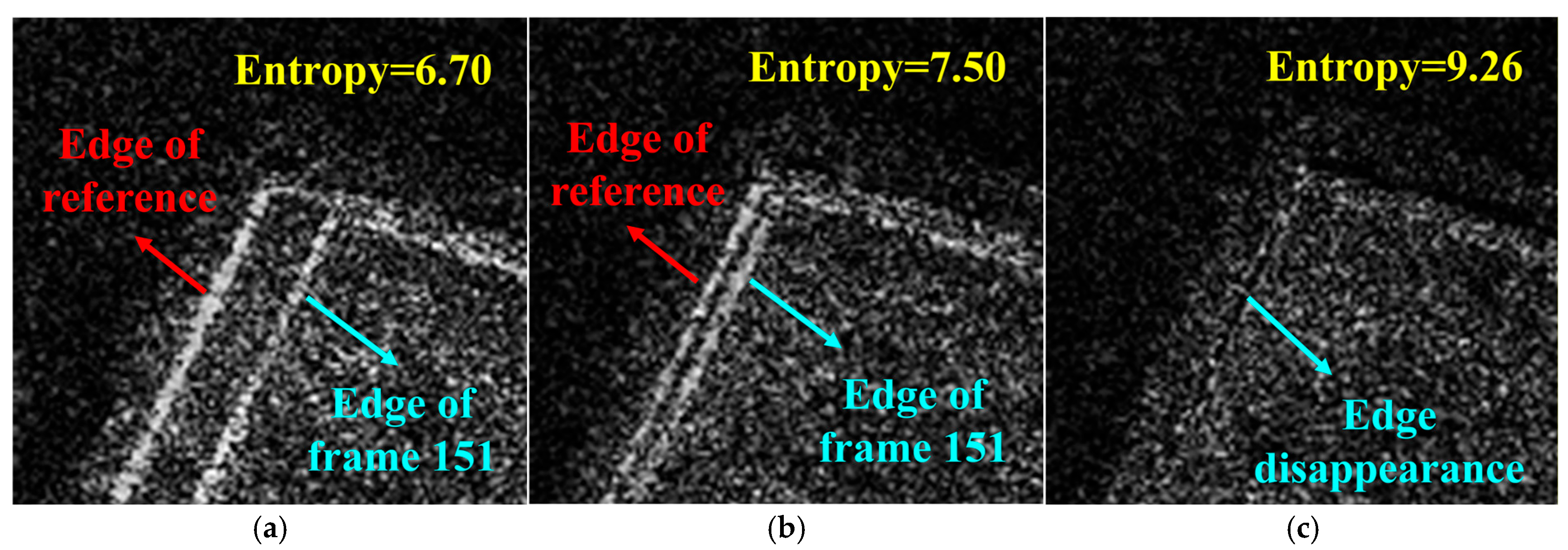
Considering that edge regions contain richer geometric information and are more sensitive to interframe drift, two regions of interest (ROIs) with clear contours and prominent features are selected from the imaging scene in Figure 4 to present the difference results. It should be noted that, if residual drift remains after image stabilization, obvious edge contours or other structural residuals still appear in the difference image, resulting in a more spatially nonuniform pixel amplitude distribution. In contrast, when the image stabilization accuracy is high, such prominent contours are greatly reduced. The difference image is then dominated by image noise, and the pixel amplitude distribution becomes more uniform. Therefore, for the resulting difference images, a larger image entropy indicates a higher ViSAR image stabilization accuracy [28].

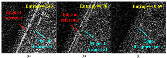
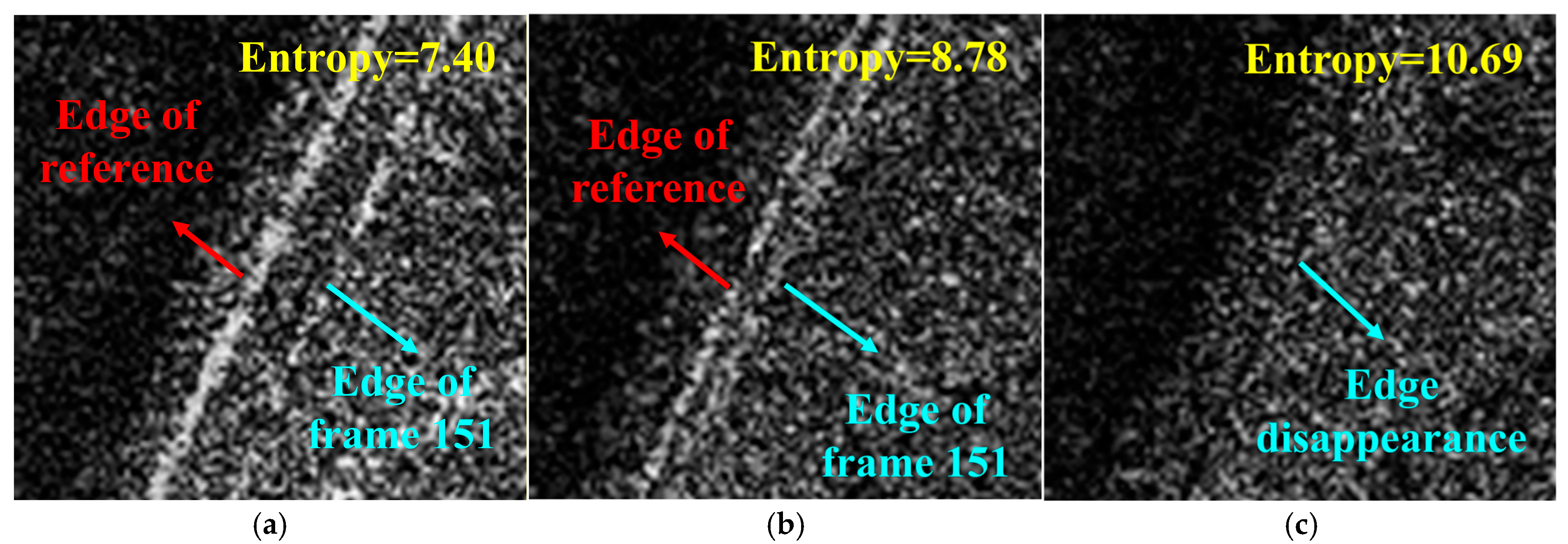
Taking frame 151 as an example, Figure 8a–c and Figure 9a–c present the difference results between the reference image and the registered image in ROI 1 and ROI 2, respectively. It can be seen that the difference images obtained from the original and NCC-registered images still contain many pixels with high amplitudes. The edge contours in these images are clearly visible, and the pixel amplitude variations exhibit a locally concentrated distribution. This indicates that the image to be registered and the reference image are not precisely aligned, causing the edge contours of both images to appear simultaneously in the difference image. In contrast, in the difference image obtained after stabilization with the proposed method, only pixels associated with image noise remain, and the overall pixel amplitude variation is more uniform.

Figure 8. Difference images for frame 151 in ROI 1. (a) Original; (b) NCC-based registration; (c) Proposed method.

Figure 9. Difference images for frame 151 in ROI 2. (a) Original; (b) NCC-based registration; (c) Proposed method.

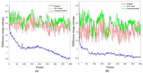
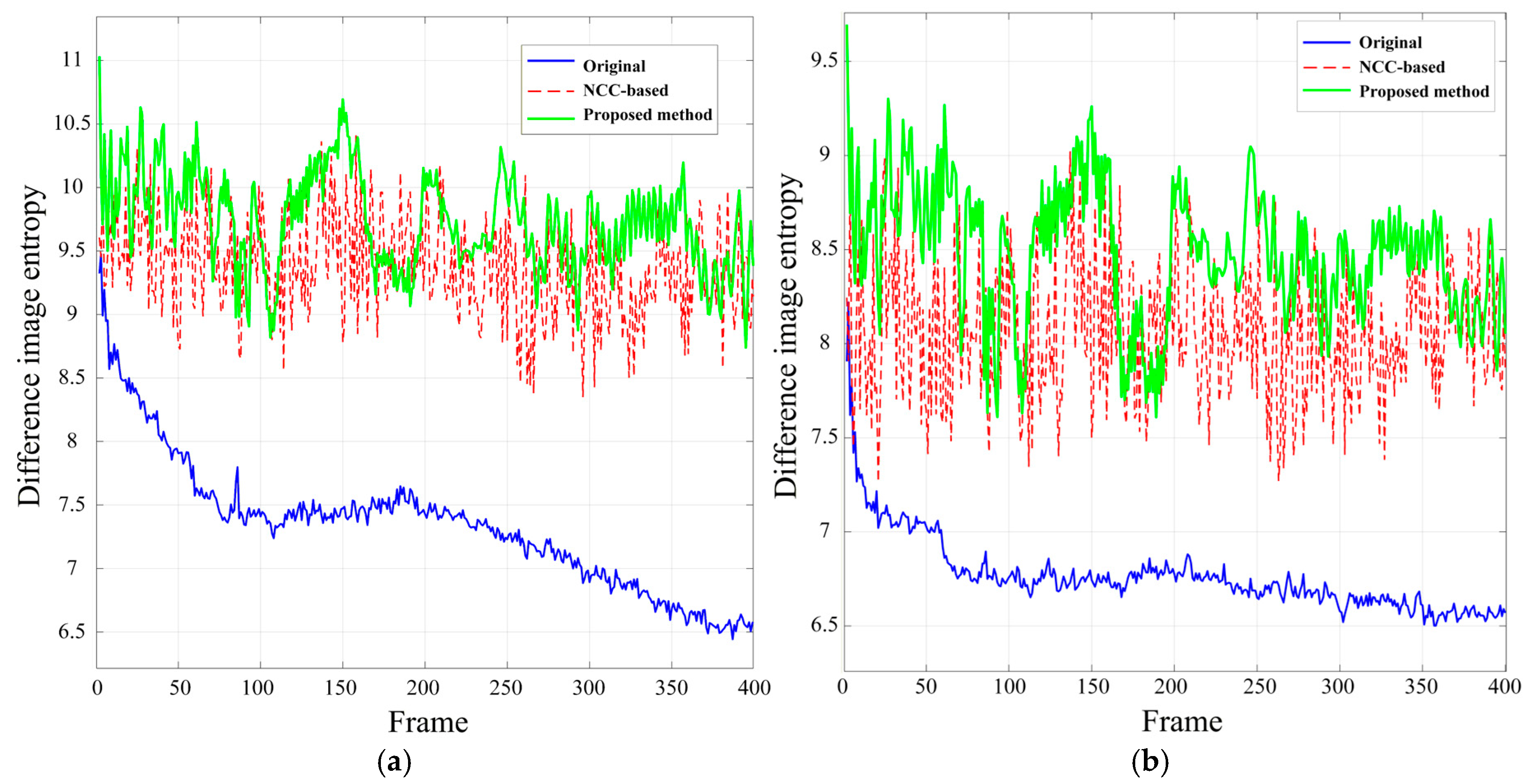
Figure 10 presents the entropy variation curves of the difference image sequences after processing by different methods. Table 4 lists the difference image entropy values of the selected frames corresponding to Figure 10. As shown in Figure 10 and Table 4, the original sequence has the smallest difference image entropy values (e.g., about 7.40 and 6.70 for ROI 1 and ROI 2, respectively, at frame 151). The entropy values increase after NCC-based registration (e.g., about 8.78 and 7.50 for ROI 1 and ROI 2, respectively, at frame 151), whereas the proposed method achieves the largest difference image entropy values in nearly all frames (e.g., about 10.69 and 9.26 for ROI 1 and ROI 2, respectively, at frame 151).

Figure 10. Entropy variation in difference image sequences. (a) ROI 1; (b) ROI 2.

Table 4. Comparison of difference image entropy for different methods.

Frame Index	Difference Image Entropy of ROI 1			Difference Image Entropy of ROI 2
	Original Sequence	NCC-Based Registration	Proposed Method	Original Sequence	NCC-Based Registration	Proposed Method
Frame 56	7.83	9.37	10.30	6.86	8.41	9.27
Frame 151	7.40	8.78	10.69	6.70	7.50	9.26
Frame 263	7.07	8.44	9.55	6.61	7.27	8.48
Frame 381	6.50	8.56	9.43	6.52	7.67	8.25

The experimental results demonstrate that the proposed Kalman filtering and smoothing strategy, based on the joint Singer-random walk model, significantly reduces the drift estimation error. For long-duration ViSAR image sequences, this approach effectively suppresses multiframe image drift and enhances the stabilization precision.

4.3. Ablation Experiments

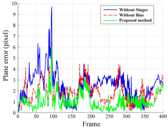
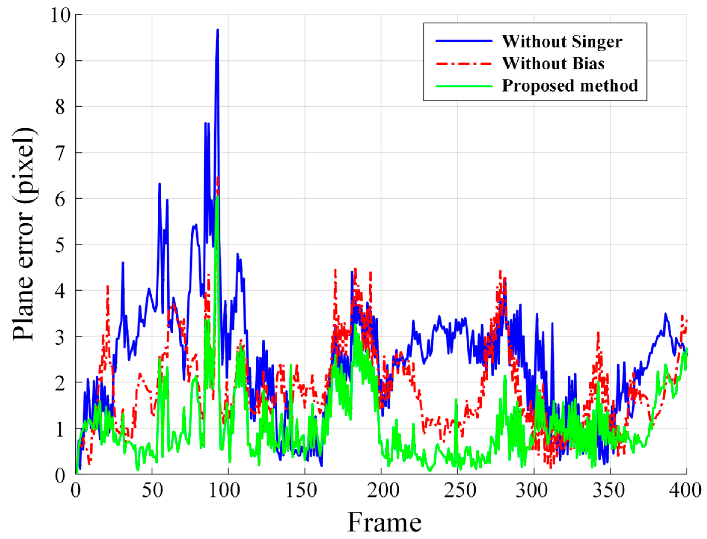
To further validate the roles of the Singer model and the random walk bias model in this paper, two ablation experiments are conducted in Section 4.3. In ablation experiment 1, the Singer model used for true drift modeling is replaced by a constant velocity (CV) model, while the bias term, Kalman filtering, and RTS smoothing are retained. In ablation experiment 2, the Singer model, Kalman filtering, and RTS smoothing are retained, but the slowly varying systematic bias is no longer modeled as a random walk process. By comparing these two ablation settings with the proposed joint model, the effects of true drift modeling and systematic bias modeling on the final stabilization performance can be evaluated.

Figure 11 presents the residual drift error curves in the two-dimensional image plane after stabilization by the three methods. As shown in Figure 11, the residual drift errors of both ablation methods increase to different degrees, whereas the proposed method yields smaller errors for most frames. This indicates that only by jointly modeling the true drift and the systematic bias can the actual drift trajectory be more accurately approximated, thereby achieving high-precision image stabilization.

Figure 11. Residual drift error in the two-dimensional image plane of ablation experiments.

Table 5 shows the RMSEs of the drift estimates for all methods over the entire frame sequence. As shown in Table 5, the two-dimensional planar RMSEs of ablation experiment 1 and ablation experiment 2 are 2.83 and 2.09 pixels, respectively, whereas that of the proposed method is further reduced to 1.31 pixels. In both the azimuth and range directions, the proposed method also achieves the lowest RMSE. These results indicate that, without the Singer model, the true drift cannot be accurately characterized, thereby degrading the final drift estimation accuracy. Moreover, without the random walk bias model, the slowly varying systematic bias contained in the NCC measurements cannot be explicitly separated, which limits the further improvement of the image stabilization accuracy. The ablation results demonstrate that the joint introduction of the Singer model and the random walk bias model is necessary for improving both drift estimation accuracy and stabilization performance.

Table 5. RMSE comparison of ablation experiments.

Direction	RMSE(400 Frames)
	Ablation Experiment 1 (Without Singer)	Ablation Experiment 2 (Without Bias)	Proposed Method
Azimuth	2.68	1.72	1.21
Range	0.90	1.20	0.51
2-D plane	2.83	2.09	1.31

5. Discussion

The comprehensive experimental evaluation reveals several significant insights into video SAR image stabilization. First, the main advantage of the proposed method over NCC-based registration is that the two-dimensional shift maximizing the NCC coefficient in each frame is treated as a drift measurement rather than the true drift. Its error is decomposed into a slowly varying systematic bias and random disturbances, where the former is modeled by a random walk process and the latter is represented as measurement noise. Moreover, NCC-based registration is essentially an independent frame-by-frame process and does not take the temporal correlation of the drift trajectory into account. In contrast, the proposed method exploits such temporal correlation in both modeling and estimation. Specifically, the true drift is represented by a two-dimensional Singer model, Kalman filtering predicts and updates the filtered state using previous frame information and NCC-based drift measurement of the current frame. Furthermore, RTS smoothing performs backward recursion on the complete filtered state sequence, thereby utilizing both past and future measurements to obtain a smoother and more accurate drift trajectory estimate.

Second, the proposed method exhibits more prominent advantages under long-time-series conditions. For short image sequences, the cumulative effect of drift error is usually not obvious. However, in experiments on long-time-series ViSAR images, the two-dimensional drift errors of the original sequence can gradually accumulate to tens of pixels. Although NCC-based registration can suppress the overall drift in long-duration image sequences, the registered sequence still exhibits pronounced interframe jitter due to errors in the NCC-based drift measurements. In contrast, the proposed method not only suppresses the overall drift, but also further reduces the residual image jitter caused by these errors. Consequently, the drift error is further constrained to the subpixel level, and the two-dimensional positional RMSE is significantly reduced. This indicates that the proposed method is particularly suitable for high-precision ViSAR image stabilization in long-duration conditions where cumulative drift and interframe jitter coexist.

Third, from the methodological perspective, the contribution of this work is not to replace NCC registration itself, but to introduce a joint state space modeling framework built upon NCC-based drift measurements. In this context, NCC-based registration is selected as the primary comparison baseline, since it is not only a representative traditional method for ViSAR image stabilization, but also the direct measurement source of the proposed state space estimation framework. Unlike approaches that directly use NCC results for image stabilization, this work focuses on a more fundamental issue: the deviation between the measurements and the true drift in long-duration ViSAR image sequences. The Singer-random walk joint model is adopted to explicitly separate the true drift from the systematic bias. Therefore, the innovation of this paper is not to redesign the image similarity criterion, but to establish a drift estimation framework with physical statistical significance for ViSAR image stabilization.

Fourth, it should be noted that the effectiveness of the proposed method is validated primarily using real W-band airborne ViSAR data. Its applicability to other frequency bands, platform motion conditions, and imaging modes remains to be further assessed. Moreover, the Singer model parameters and noise covariance matrices are currently specified manually. It is necessary to investigate adaptive parameter estimation methods in future work to enhance the generalization capability of the algorithm. Comparisons with more advanced feature-based or learning-based registration methods will also be considered in future work. Furthermore, the proposed method is essentially an image domain approach that performs stabilization after image formation. Future work may consider modeling drift error in the signal domain and conducting drift estimation and compensation during the multiframe imaging process, so as to directly generate continuous and stable ViSAR image sequence. However, drift error in the raw echo data is typically time-varying, and its precise modeling and robust estimation still require further research.

6. Conclusions

To address the issues of interframe drift and insufficient stabilization accuracy in long-duration airborne video SAR image sequences, this paper proposes a ViSAR image stabilization method based on a joint Singer-random walk model. Compared with the conventional image registration algorithm based on NCC, the proposed method models the true drift and systematic bias in the state space separately, and applies Kalman filtering followed by RTS smoothing to the NCC-based drift measurements over the entire frame sequence. This yields a smoother two-dimensional drift estimate that is closer to the real drift trajectory, which is then used to perform frame-by-frame subpixel drift correction of the original ViSAR image sequence. The experimental results based on real airborne ViSAR data demonstrate that the proposed algorithm is significantly superior to the NCC registration method in multiframe image stabilization performance. Local image comparisons show that the stationary point targets can be aligned to the same pixel position across consecutive frames after processing by our method, and interframe drift and jitter are effectively suppressed. Quantitative analyses of the control point residual drift errors and the difference image entropy further confirm that our approach simultaneously reduces both the fluctuation and the RMSE of the drift estimates, while maintaining the largest difference image entropy in each frame, thereby enhancing scene stability and stabilization precision in multiframe ViSAR imaging.

References

- Fan, L.; Wang, H.; Yang, Q.; Deng, B. High-Quality Airborne Terahertz Video SAR Imaging Based on Echo-Driven Robust Motion Compensation. IEEE Trans. Geosci. Remote Sens. 2024, 62, 1–17. [Google Scholar] [CrossRef] [Scilit]
- Gao, A.; Sun, B.; Guo, Y.; Li, J.; Li, C.; Chen, X. A Parameter-Adjusting Auto-Registration Overlapped Subaperture Algorithm for Video Synthetic Aperture Radar Imaging. IEEE Trans. Geosci. Remote Sens. 2023, 61, 1–14. [Google Scholar] [CrossRef] [Scilit]
- Chen, Q.; Liu, Y.; Wang, L.; Yu, Z. W-band airborne video synthetic aperture radar system. J. Terahertz Sci. Electron. Inf. Technol. 2024, 22, 46–53. [Google Scholar]
- Yan, S.; Fu, Y.; Zhang, W.; Yang, W.; Yu, R.; Zhang, F. Review of the development status for ViSAR techniques. Syst. Eng. Electron. 2024, 46, 2650–2666. [Google Scholar]
- Zhang, Y.; Ding, D.Z.; Wang, P.; Leung, H. Video Synthetic Aperture Radar Techniques: A retrospective and prospective overview. IEEE Geosci. Remote Sens. Mag. 2025, 13, 468–495. [Google Scholar] [CrossRef] [Scilit]
- Yan, H.; Liu, H.; Xu, X.; Zhou, Y.; Cheng, L.; Li, Y.; Wu, D.; Zhang, J.; Wang, L.; Zhu, D. A New Method of Video SAR Ground Moving Target Detection and Tracking Based on the Interframe Amplitude Temporal Curve. IEEE Trans. Geosci. Remote Sens. 2023, 61, 1–17. [Google Scholar] [CrossRef] [Scilit]
- Ding, J.; Zhong, C.; Wen, L.; Xu, Z. Joint detection of moving target in video synthetic aperture radar. J. Radars 2022, 11, 313–323. [Google Scholar]
- Linnehan, R.; Miller, J.; Asadi, A. Map-drift autofocus and scene stabilization for video-SAR. In Proceedings of the 2018 IEEE Radar Conference (RadarConf18), Oklahoma City, OK, USA, 23–27 April 2018; pp. 1401–1405. [Google Scholar]
- Etezadifar, P.; Farsi, H. A New Sample Consensus Based on Sparse Coding for Improved Matching of SIFT Features on Remote Sensing Images. IEEE Trans. Geosci. Remote Sens. 2020, 58, 5254–5263. [Google Scholar] [CrossRef] [Scilit]
- Dellinger, F.; Delon, J.; Gousseau, Y.; Michel, J.; Tupin, F. SAR-SIFT: A SIFT-Like Algorithm for SAR Images. IEEE Trans. Geosci. Remote Sens. 2015, 53, 453–466. [Google Scholar] [CrossRef] [Scilit]
- Lowe, D.G. Distinctive Image Features from Scale-Invariant Keypoints. Int. J. Comput. Vis. 2004, 60, 91–110. [Google Scholar] [CrossRef] [Scilit]
- Zhu, Y.; Guo, C. The research of correlation matching algorithm based on correlation coefficient. J. Signal Process. 2003, 19, 531–534. [Google Scholar]
- Wang, Y.; Yu, Q.; Yu, W. An improved Normalized Cross Correlation algorithm for SAR image registration. In Proceedings of the 2012 IEEE International Geoscience and Remote Sensing Symposium, Munich, Germany, 22–27 July 2012; pp. 2086–2089. [Google Scholar]
- Pallotta, L.; Giunta, G.; Clemente, C. Subpixel SAR Image Registration Through Parabolic Interpolation of the 2-D Cross Correlation. IEEE Trans. Geosci. Remote Sens. 2020, 58, 4132–4144. [Google Scholar] [CrossRef] [Scilit]
- Singer, R.A. Estimating Optimal Tracking Filter Performance for Manned Maneuvering Targets. IEEE Trans. Aerosp. Electron. Syst. 1970, AES-6, 473–483. [Google Scholar] [CrossRef] [Scilit]
- Li, Y.; Zhang, J. Real-time error registration algorithm and analysis based on the SINGER model. Syst. Eng. Electron. 2015, 37, 1255–1258. [Google Scholar]
- Zhang, T. Research on Maneuvering Multi-Target Tracking Based on Stationary Singer Motion Model. Master’s Thesis, Xidian University, Xi’an, China, 2023. [Google Scholar]
- Ren, Y.; Tang, S.; Guo, P.; Zhang, L.; So, H.C. 2-D Spatially Variant Motion Error Compensation for High-Resolution Airborne SAR Based on Range-Doppler Expansion Approach. IEEE Trans. Geosci. Remote Sens. 2022, 60, 5201413. [Google Scholar] [CrossRef] [Scilit]
- Zeng, L.; Liang, Y.; Xing, M.; Huai, Y.; Li, Z. A Novel Motion Compensation Approach for Airborne Spotlight SAR of High-Resolution and High-Squint Mode. IEEE Geosci. Remote Sens. Lett. 2016, 13, 429–433. [Google Scholar] [CrossRef] [Scilit]
- Huang, Y.; Liu, F.; Chen, Z.; Li, J.; Hong, W. An Improved Map-Drift Algorithm for Unmanned Aerial Vehicle SAR Imaging. IEEE Geosci. Remote Sens. Lett. 2021, 18, 1–5. [Google Scholar] [CrossRef] [Scilit]
- Wei, S.; Zhang, L.; Liu, H. Integrated Kalman Filter of Accurate Ranging and Tracking With Wideband Radar. IEEE Trans. Geosci. Remote Sens. 2020, 58, 8395–8411. [Google Scholar] [CrossRef] [Scilit]
- Joshi, S.K.; Baumgartner, S.V.; Krieger, G. Tracking and Track Management of Extended Targets in Range-Doppler Using Range-Compressed Airborne Radar Data. IEEE Trans. Geosci. Remote Sens. 2022, 60, 5102720. [Google Scholar] [CrossRef] [Scilit]
- Lai, F. Research on Maneuvering Target Tracking Methods. Master’s Thesis, Xidian University, Xi’an, China, 2020. [Google Scholar]
- Liang, Y.; Li, Z.; Zeng, L.; Xing, M.; Bao, Z. A High-Order Phase Correction Approach for Focusing HS-SAR Small-Aperture Data of High-Speed Moving Platforms. IEEE J. Sel. Top. Appl. Earth Obs. Remote Sens. 2015, 8, 4551–4561. [Google Scholar] [CrossRef] [Scilit]
- Brown, W.M. SAR resolution in the presence of phase errors. IEEE Trans. Aerosp. Electron. Syst. 1988, 24, 808–814. [Google Scholar] [CrossRef] [Scilit] [PubMed]
- Wahl, D.E.; Eichel, F.H.; Ghiglia, D.C.; Jakowatz, C.V. Phase gradient autofocus-a robust tool for high resolution SAR phase correction. IEEE Trans. Aerosp. Electron. Syst. 1994, 30, 827–835. [Google Scholar] [CrossRef] [Scilit]
- Wang, L.; Xiang, W.; Song, H.; Zhang, H.; Zheng, M.; Wang, J.; Xue, F.; Ai, Z.; Deng, Y. A Novel Phase Calibration Method for Airborne P-, L-, and S-Band SAR Tomography Based on Weighted Phase Gradient Autofocus. IEEE Trans. Geosci. Remote Sens. 2025, 63, 5223920. [Google Scholar] [CrossRef] [Scilit]
- Zhang, Q.; Li, S.; Cheng, L.; Shang, S.; Teng, F.; Sun, J. A Novel Circular SAR Subaperture Image Registration Method Based on Accelerated-KAZE. In Proceedings of the 2025 IEEE 8th International Conference on Computer and Communication Engineering Technology (CCET), Beijing, China, 15–17 August 2025; pp. 207–212. [Google Scholar]
Disclaimer/Publisher’s Note: The statements, opinions and data contained in all publications are solely those of the individual author(s) and contributor(s) and not of MDPI and/or the editor(s). MDPI and/or the editor(s) disclaim responsibility for any injury to people or property resulting from any ideas, methods, instructions or products referred to in the content. |
© 2026 by the authors. Licensee MDPI, Basel, Switzerland. This article is an open access article distributed under the terms and conditions of the Creative Commons Attribution (CC BY) license.