Fast Low-Artifact Image Generation for Staggered SAR: A Preview-Oriented Method

Highlights

What are the main findings?

• A three-stage processing framework is proposed to efficiently suppress azimuth artifacts in low-oversampled staggered SAR.
• The method achieves imaging quality comparable to precise reconstruction approaches while significantly reducing computational cost.

What are the implications of the main findings?

• Enables fast generation of low-artifact images for wide-area staggered SAR scene screening.
• Provides an efficient front-end imaging solution that supports early decision-making.

Abstract

Staggered synthetic aperture radar (SAR) is an innovative concept capable of achieving an ultrawide continuous swath with fine azimuth resolution by variable pulse repetition interval. However, the inherent data gaps and nonuniform sampling introduce severe azimuth artifacts, degrading image quality. Existing methods can mitigate these artifacts but struggle to effectively balance imaging quality and computational cost, especially under low oversampling conditions. To address this challenge, this paper proposes a low-artifact preview image generation method for staggered SAR. First, the artifact characteristics are analyzed through the derivation of a staggered SAR signal model. Then, a three-stage processing framework is introduced, consisting of constant-gradient phase extrapolation, artifact-based inverse filtering, and result fusion. Additionally, data nonuniformity is addressed using a weighted nonuniform fast Fourier transform. Simulation results demonstrate that the proposed method significantly improves processing speed compared to existing techniques while maintaining good imaging quality, making it suitable for rapid scene screening in wide-area SAR applications.

1. Introduction

Synthetic aperture radar (SAR) is a powerful tool for Earth observation that is unaffected by extreme weather conditions [1]. It supports a wide range of applications across multiple scales, from large-area environmental monitoring to fine-resolution target analysis, and from population-level observations to individual object detection, demonstrating its broad versatility [2,3,4]. Achieving simultaneously high resolution and wide swath (HRWS) has long been regarded as a key development direction in SAR [5]. This capability makes HRWS SAR particularly suitable for marine applications, where wide-area situational awareness and fine-scale target characterization are both required. Recent studies have shown that HRWS SAR data can effectively support maritime tasks such as ship detection, classification, and large-scale ocean monitoring. Representative works include balance-learning-based ship detection methods, polarization-fusion frameworks for robust ship classification, and high-performance models such as HyperLi-Net, highlighting the practical value of HRWS SAR in operational marine scenarios [6,7,8].

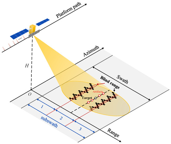
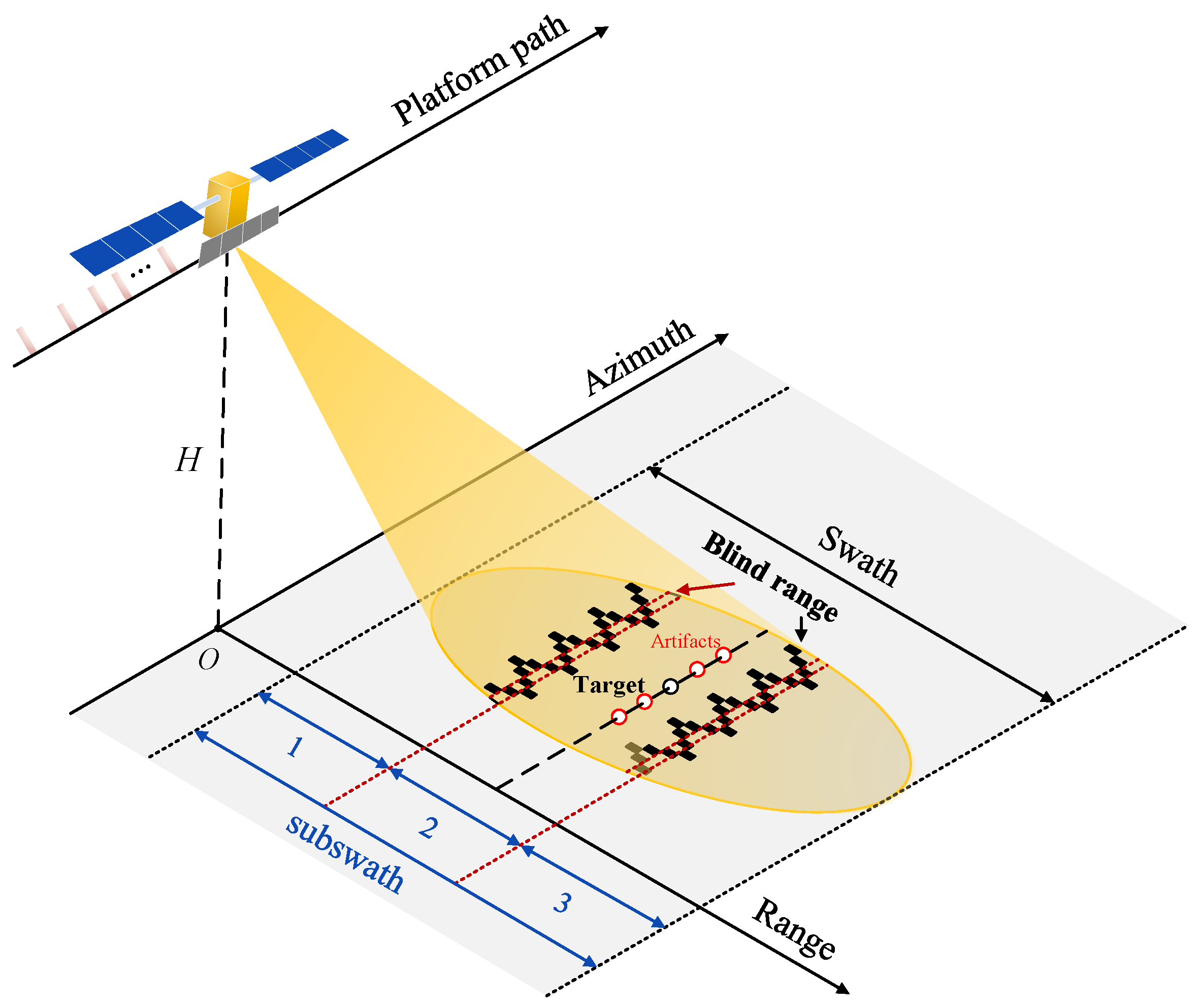
In particular, ultrawide-swath imaging enables simultaneous coverage of multiple regions, increasing the revisit frequency for specific areas and facilitating rapid response to unforeseen events [9,10]. Traditional wide-swath modes, including ScanSAR and terrain observation by progressive scans (TOPS), inevitably sacrifice azimuth resolution [11,12,13]. The application of azimuth multichannel techniques for ScanSAR and TOPS partially alleviates this limitation but suffers from Doppler centroid diversity across channels [14,15]. Alternatively, digital beamforming (DBF) in elevation provides wide-swath coverage by simultaneously imaging multiple subswaths, but blind ranges arise from transmit-receive conflicts [16]. To overcome these drawbacks, staggered SAR was introduced, exploiting variable pulse repetition interval (PRI) to address the fixed blind range problem and achieve a continuous ultrawide swath [17,18].

While staggered acquisition enables continuous imaging, it also introduces data nonuniformity and gaps along the swath. If not properly addressed, these factors lead to pronounced azimuth artifacts on the staggered SAR image and make image quality highly dependent on the signal processing scheme. Early studies proposed one-step approaches, such as two-point linear interpolation, multichannel reconstruction (MCR), and best linear unbiased (BLU) interpolation [18]. These methods directly resample the data on a uniform grid, resulting in a low computational burden, and are therefore referred to as fast methods. However, they require a high oversampling ratio, typically around 2 [18,19,20], to effectively suppress azimuth artifacts. Here, the oversampling ratio refers to the ratio between the average pulse repetition frequency (PRF) and the Doppler bandwidth. Excessively high PRF can degrade the range ambiguity performance and increase the system data burden, making them impractical in real systems. Despite this, staggered SAR is considered the baseline acquisition mode for Tandem-L [20]. Due to data rate limitations, the NASA-ISRO SAR (NISAR) operates at a relatively low PRF, which sparked extensive discussions on low oversampling conditions, typically with oversampling ratios of about 1.1 to 1.3 [21,22,23,24,25].

To address the performance degradation of fast methods in low-oversampled staggered SAR, more advanced approaches have been explored. For instance, ref. [26] proposed a two-step framework, in which data gaps are first recovered using the missing data iterative adaptive approach (MIAA). In the second step, resampling is performed using MCR [18,27] or BLU [28,29], achieving improved imaging quality at the cost of increased signal processing complexity. Further studies within the two-step framework have focused on continuous improvements in gap recovery. For example, linear Bayesian estimation (LBE) and its improved version (ILBE) exploit autocorrelation-based linear prediction [30], while matrix completion (MC) uses nuclear norm minimization to reconstruct missing data [31]. The common limitation of these approaches is their highly complex matrix operations, which lead to excessive time consumption in data recovery. The aforementioned approaches can all be classified as precise methods. In parallel, methods based on compressive sensing (CS) imaging have been widely applied to image reconstruction in low-oversampled staggered SAR [32,33,34]. However, such CS-based approaches, which rely on sparsity priors, are also hindered by prolonged reconstruction time.

Overall, the central challenge remains the trade-off between imaging quality and computational cost: fast methods offer low computational complexity but result in poor image quality under low-oversampled conditions, whereas precise methods achieve high-quality recovery at the cost of extended processing times, while staggered SAR can acquire ultrawide-swath images in a single pass, enabling large-area coverage and rapid response, this trade-off limits its effectiveness for time-critical applications requiring artifact-free or low-artifact images, such as disaster monitoring and emergency response. Consequently, developing a processing framework that balances quality and efficiency is still an issue for low-oversampled staggered SAR.

To address this challenge, this paper proposes a low-artifact preview image generation method for low-oversampled staggered SAR, aiming to support rapid scene interpretation and screening at a low computational cost. The proposed method consists of three processing stages in total. The main contributions of this paper are as follows.

• The characteristics of azimuth artifacts are analyzed by establishing a staggered SAR signal model that accounts for data gaps and nonuniformity, providing a foundation for subsequent signal processing.
• A low-artifact preview image generation method is proposed for low-oversampled staggered SAR, employing a three-stage processing framework. In the first two stages, data gaps are recovered via constant-gradient phase extrapolation (CGPE) and artifact-based inverse filtering (ABIF), each producing an independent imaging result. The data nonuniformity in both stages is addressed using the weighted nonuniform fast Fourier transform (NUFFT) technique. The final stage fuses the two results to achieve comprehensive artifact suppression across the entire scene.
• The performance of the method is validated through simulations of the point and distributed target. Experimental results demonstrate that the proposed method not only excels among fast methods but also achieves the fastest speed among precise methods with better imaging quality, making it well-suited for preview applications.

The rest of the paper is organized as follows. Section 2 analyzes the characteristics of azimuth artifacts and introduces the basic principles of the data recovery method, including CGPE and ABIF. Section 3 provides the three-stage processing framework for generating low-artifact preview images. In Section 4, simulations with different scenarios are concerned to validate the effectiveness of the proposed method. The computational complexity of the proposed method is analyzed in Section 5. Finally, Section 6 draws conclusions based on the findings.

2. Data Recovery Principle

In this section, we establish a model for staggered SAR to examine the characteristics of azimuth artifacts. The two key components of the proposed method, CGPE and ABIF, are then explored in detail. Both aim to recover data gaps but operate on different principles. The CGPE achieves signal estimation by focusing on specific signal characteristics, while the ABIF accomplishes data recovery via inverse-matched filtering.

2.1. Azimuth Artifact Analysis

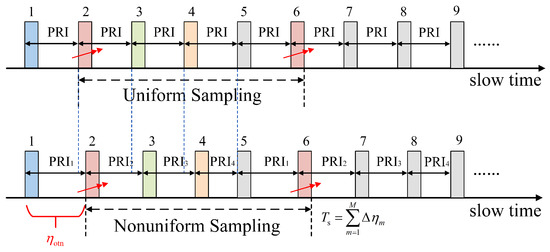
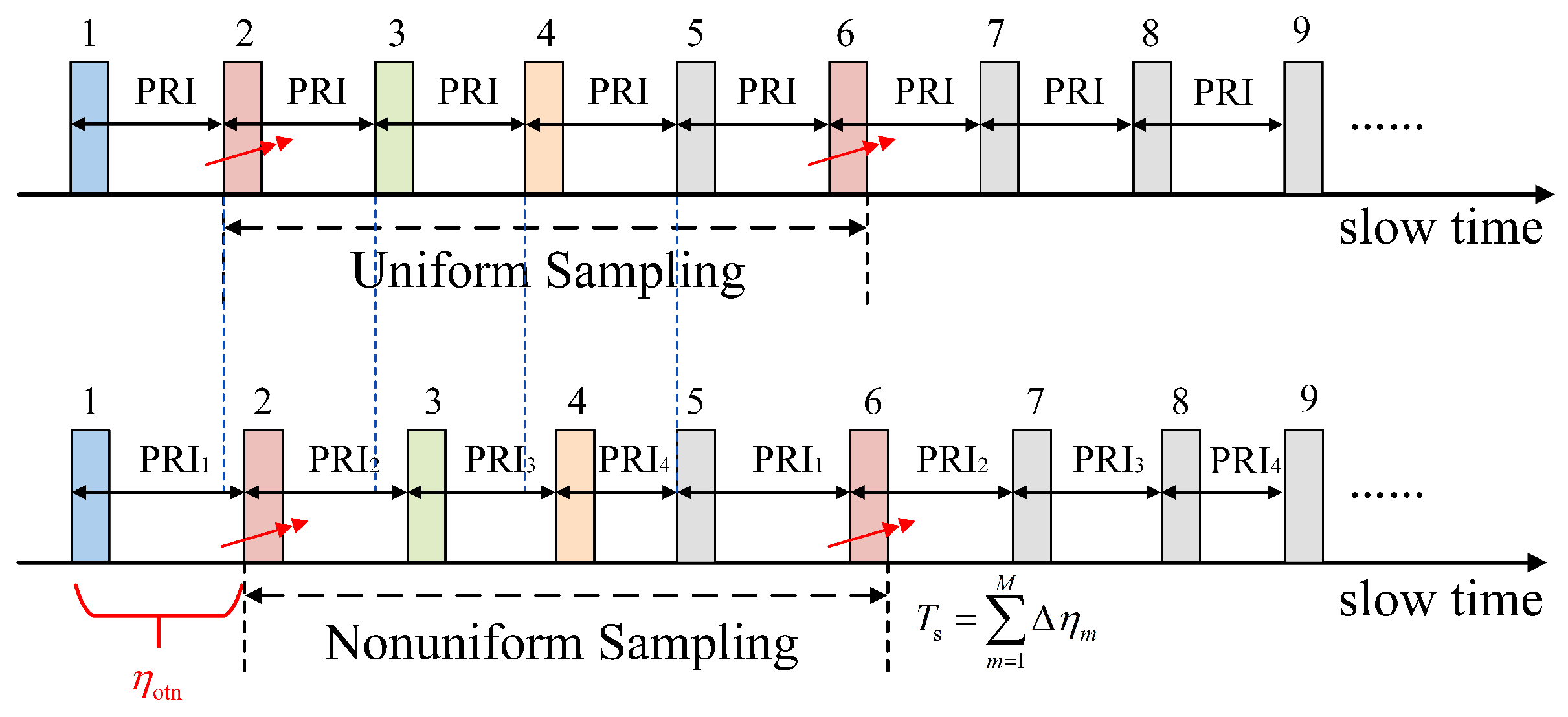
The staggered SAR systems transmit linear frequency modulation (LFM) signals at nonuniform time intervals determined by a designed PRI sequence. The corresponding operation mode is illustrated in Figure 1. Suppose the PRI sequence is periodic with a period of M and the PRI values within one period are denoted as $\mathrm{PR}{\mathrm{I}}_1,\mathrm{PR}{\mathrm{I}}_2,\dots ,\mathrm{PR}{\mathrm{I}}_M$ (abbreviated as $\Delta {\eta }_1,\dots ,\Delta {\eta }_M$).

Figure 1. Schematic diagram of staggered SAR operation mode.

Given that the primary distinction of staggered SAR lies in its azimuth sampling structure, the analysis is conducted using one-dimensional (1-D) azimuth signals for clarity. Assume the antenna is weighed via a rectangular window for ease of derivation. Consequently, the signal backscattered from the target is obtained by

$$s\left(\eta \right)=\sigma ·\mathrm{rect}\left[{\displaystyle \frac{\eta -{\eta }_{\mathrm{c}}}{T_{\mathrm{a}}}}\right]·exp\left(-j{\displaystyle \frac{4\pi R_0}{\lambda }}-j\pi K_{\mathrm{a}}{\eta }^2\right)$$

(1)

where $\sigma$ is the backscattering coefficient, $\eta$ and ${\eta }_c$, respectively, represent slow time in azimuth and the beam center time. $T_{\mathrm{a}}$ is the synthetic aperture time, $R_0$ denotes the minimum slant range, j is the imaginary unit, $\lambda$ is the carrier wavelength. $K_{\mathrm{a}}$ represents the azimuth chirp rate, which approximately satisfies $K_{\mathrm{a}}\approx 2V_{\mathrm{r}}^2/\phantom{2V_{\mathrm{r}}^2\lambda R_0}\lambda R_0$, and $V_{\mathrm{r}}$ is the equivalent radar speed.

First, the impact of nonuniform transmission timing on the staggered SAR system will be analyzed. Define a nonuniform sampling function [24] as

$$\begin{array}{cc}\hfill p_{\mathrm{non}}\left(\eta \right)=& \sum _{n=-N/2}^{N/2-1}\delta \left(\eta -n{T}_{\mathrm{u}}\right)+\delta \left(\eta -n{T}_{\mathrm{u}}-\Delta {\eta }_1\right)+\hfill \\ \hfill & \dots +\delta \left(\eta -n{T}_{\mathrm{u}}-\left(\Delta {\eta }_1+\dots +\Delta {\eta }_{M-1}\right)\right).\hfill \end{array}$$

(2)

Among them, N is the ratio of the total azimuth samples $N_{\mathrm{a}}$ to the PRI period, that is, $N=⌊N_{\mathrm{a}}/\phantom{N_{a}M}M⌋$, where $⌊·⌋$ denotes the floor function. $T_{\mathrm{u}}$ represents the period of the nonuniform sampling function, satisfying $T_{\mathrm{u}}={\sum }_{m=1}^M\Delta {\eta }_m$. If the data gaps are disregarded firstly, the nonuniform signal $s_{\mathrm{non}}\left(\eta \right)$ can be considered as the result of sampling the continuous signal $s\left(\eta \right)$ using this function, that is $s_{\mathrm{non}}\left(\eta \right)=s\left(\eta \right)·p_{\mathrm{non}}\left(\eta \right)$. The frequency domain form of $s_{\mathrm{non}}\left(\eta \right)$ is

$$\begin{array}{cc}\hfill S_{\mathrm{non}}\left(f_{\eta }\right)& =S\left(f_{\eta }\right)\otimes P_{\mathrm{non}}\left(f_{\eta }\right)\hfill \\ \hfill & =S\left(f_{\eta }\right)\otimes \sum _{n=-N/2}^{N/2-1}{M}_n·\delta \left(f_{\eta }-n{f}_{\mathrm{u}}\right)\hfill \\ \hfill & =\sum _{n=-N/2}^{N/2-1}{M}_n·S\left(f_{\eta }-n{f}_{\mathrm{u}}\right)\hfill \end{array}$$

(3)

where ⊗ is a convolution operation. $f_{\eta }$ is the Doppler frequency, $f_{\mathrm{u}}$ is the frequency of the nonuniform sampling function, satisfying $f_{\mathrm{u}}=1/\phantom{1T_{\mathrm{u}}}{T}_{\mathrm{u}}=\mathrm{PR}{\mathrm{I}}_{\mathrm{mean}}/\phantom{\mathrm{PR}{\mathrm{I}}_{\mathrm{mean}}M}M$, where $\mathrm{PR}{\mathrm{I}}_{\mathrm{mean}}$ denotes the mean PRI over one period. The expression of $M_n$ is

$$\begin{array}{cc}\hfill M_n=f_{\mathrm{u}}·& [1+e^{-j2\pi n{f}_{\mathrm{u}}\Delta {\eta }_1}+e^{-j2\pi n{f}_{\mathrm{u}}\left(\Delta {\eta }_1+\Delta {\eta }_2\right)}+\dots \hfill \\ & +e^{-j2\pi n{f}_{\mathrm{u}}\left(\Delta {\eta }_1+\dots +\Delta {\eta }_{M-1}\right)}].\hfill \end{array}$$

(4)

Now, take data gaps into consideration, whose distribution characteristics are determined by the PRI sequence design criteria. Existing PRI sequences include slow PRI variation [17], fast PRI variation [18], stepped PRI variation [30], elaborated PRI variation [18], and nonlinear PRI variation [33]. Among these designs, the slow PRI variation tends to produce continuous data gaps, which significantly degrade image quality [35,36]. In contrast, other PRI designs are generally formulated to avoid consecutive azimuth sample losses within each period, thereby facilitating efficient data recovery. Suppose one out of every M signal samples is missing. Analogous to the nonuniform sampling function, a missing sampling function is introduced and can be expressed

$$p_{\mathrm{b}}\left(\eta \right)=\mathrm{rect}\left[{\displaystyle \frac{\eta }{T}}\right]\otimes \sum _{n=-N/2}^{N/2-1}\delta \left(\eta -{\eta }_{\mathrm{otn}}-n{T}_{\mathrm{s}}\right)$$

(5)

where T and $T_{\mathrm{s}}$ correspond to the pulse width and the period of the missing sampling function. Whether it is the nonuniform sampling function or the missing sampling function, both share the same period equal to the sum of one PRI period, satisfying $T_{\mathrm{u}}=T_{\mathrm{s}}$. ${\eta }_{\mathrm{otn}}$ denotes the missing sampling offset time, which satisfies ${\eta }_{\mathrm{otn},i}={\sum }_{m=0}^{i-1}\Delta {\eta }_m$ (suppose that $\Delta {\eta }_0=0$), where $i=1,\dots ,M$ is the index of the missing pulse within the PRI period. It denotes the time offset of the missing data within a PRI period relative to the start of that period. As illustrated in Figure 2, taking the PRIs with period $M=4$ (with larger values in practice) as an example, the 2nd sample is missing in each period, satisfying ${\eta }_{\mathrm{otn}}=\Delta {\eta }_1$.

Figure 2. Diagram of missing sampling offset time in nonuniform data, where pulses marked with red double arrows indicate the presence of data gaps.

Although signal lost in staggered SAR occur on a nonuniform sampling basis, the missing data (i.e., data gaps) $s_{\mathrm{b}}\left(\eta \right)$ itself can be treated as uniformly sampled. Assume ${\eta }_{\mathrm{otn}}=0$, which means the first sample missed within each PRI period. Thus, the missing data can be expressed as

$$\begin{array}{cc}\hfill s_{\mathrm{b}}\left(\eta \right)=& s\left(\eta \right)·p_{\mathrm{non}}\left(\eta \right)·p_{\mathrm{b}}\left(\eta \right)=s\left(\eta \right)·p_{\mathrm{b}}\left(\eta \right)\hfill \\ \hfill =& s\left(\eta \right)·\left\{\mathrm{rect}\left[{\displaystyle \frac{\eta }{T}}\right]\otimes \sum _{n=-N/2}^{N/2-1}\delta \left(\eta -n{T}_{\mathrm{s}}\right)\right\}.\hfill \end{array}$$

(6)

The frequency domain form of $s_{\mathrm{b}}\left(\eta \right)$ is

$$\begin{array}{cc}\hfill S_{\mathrm{b}}\left(f_{\eta }\right)=& S\left(f_{\eta }\right)\otimes P_{\mathrm{b}}\left(f_{\eta }\right)\hfill \\ \hfill =& S\left(f_{\eta }\right)\otimes \sum _{n=-N/\phantom{N2}2}^{N/\phantom{N2-1}2-1}{b}_n·\delta \left(f-n{f}_{\mathrm{s}}\right)\hfill \\ \hfill =& \sum _{n=-N/\phantom{N2}2}^{N/\phantom{N2-1}2-1}{b}_n·S\left(f-n{f}_{\mathrm{s}}\right)\hfill \end{array}$$

(7)

where $b_n=T{f}_{\mathrm{s}}\mathrm{sinc}\left(n{f}_{\mathrm{s}}T\right)$, $f_{\mathrm{s}}$ is the frequency of the missing sampling function fulfilling $f_{\mathrm{s}}=1/T_{\mathrm{s}}=1/T_{\mathrm{u}}=f_{\mathrm{u}}$.

Therefore, the time-domain signal model of staggered SAR is $s_{\mathrm{non},\mathrm{m}}\left(\eta \right)=s_{\mathrm{non}}\left(\eta \right)+\left[-s_{\mathrm{b}}\left(\eta \right)\right]$. The uniformly sampled signal without data gaps is defined as the reference signal, and the image obtained by compressing this reference signal is referred to as the main image. However, the signal of staggered SAR does not match the matching filter of the reference signal. Therefore, we obtain

$$\begin{array}{cc}\hfill & y_{\mathrm{non},\mathrm{m}}\left(\eta \right)=\sigma ·exp\left(-j{\displaystyle \frac{4\pi R_0}{\lambda }}\right)exp\left(j2\pi f_{{\eta }_{\mathrm{c}}}\eta \right)\hfill \\ \hfill & ·\left\{\sum _{n=-N/2}^{N/2-1}\left(M_n+b_n\right)E_n{B}_{\mathrm{a}}\mathrm{sinc}\left[\left(\eta -{\displaystyle \frac{n{f}_{\mathrm{s}}}{K_{\mathrm{a}}}}\right)B_{\mathrm{a}}\right]\right\}\hfill \end{array}$$

(8)

with

$$E_n=exp\left[j\pi {\displaystyle \frac{{\left(n{f}_{\mathrm{s}}\right)}^2}{K_{\mathrm{a}}}}\right]·exp\left(-j2\pi f_{{\eta }_c}{\displaystyle \frac{n{f}_{\mathrm{s}}}{K_{\mathrm{a}}}}\right).$$

(9)

Among them, $f_{{\eta }_{\mathrm{c}}}$ is the Doppler center frequency, $B_{\mathrm{a}}$ is the Doppler bandwidth. The above analysis indicates that staggered SAR signals produce multiple pairs of azimuth artifacts after compression, with their intensity proportional to the target backscattering coefficient. These artifacts are uniformly spaced, with the interval determined by the ratio of the missing (or nonuniform) sampling frequency to the azimuth chirp rate, given by $f_{\mathrm{s}}/\phantom{n{f}_{\mathrm{s}}{K}_a}{K}_{\mathrm{a}}$.

2.2. Constant-Gradient Phase Extrapolation (CGPE)

The most visually prominent artifacts in images of staggered SAR typically arise from strong-scattering structures, such as dihedral or trihedral configurations. These structures appear as point-like targets with high backscattering coefficients, which markedly influence image interpretation. As shown in (8), the artifact intensity increases with the target’s backscattering coefficient. Consequently, artifacts caused by such targets are not only intense but also spread over a broad azimuth range, making them particularly conspicuous in high-contrast regions [29]. In these scenarios, strong point-like targets dominate the artifact pattern, while artifacts from weaker scatterers are often masked by noise.

To address the data gaps that give rise to such artifacts, the CGPE method is employed. CGPE assumes that the phase of SAR signals within a local region exhibits a constant gradient, i.e., the phase behaves as a locally linear feature. The method estimates the local phase gradient from adjacent valid samples and linearly extrapolates the phase into the gap. The amplitude at the missing positions is approximated by averaging the adjacent values on either side of the gap.

Unlike the two-point linear interpolation that directly interpolates the complex signal, the CGPE method separately recovers the phase and amplitude based on the signal characteristics. In cases dominated by isolated strong point-like targets, the local phase remains approximately linear, and CGPE can achieve nearly perfect recovery with low computational cost. However, in scenes containing complex distributed targets, the phase may deviate from local linearity, reducing the effectiveness of CGPE. Therefore, further processing is required to suppress artifacts resulting from targets that do not conform to local linear phase characteristics.

2.3. Artifact-Based Inverse Filtering (ABIF)

The traditional methods, such as those based on spectral sparsity or low-rank priors, achieve data recovery by exploiting inherent signal structures. However, they typically require multiple iterations, leading to relatively high computational costs and prolonged recovery times. In contrast, the proposed ABIF method capitalizes on the structural characteristics of the artifacts themselves to complete data recovery. This subsection provides a detailed analysis of the ABIF principle.

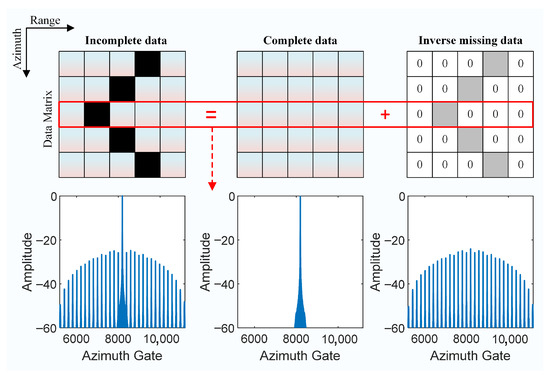
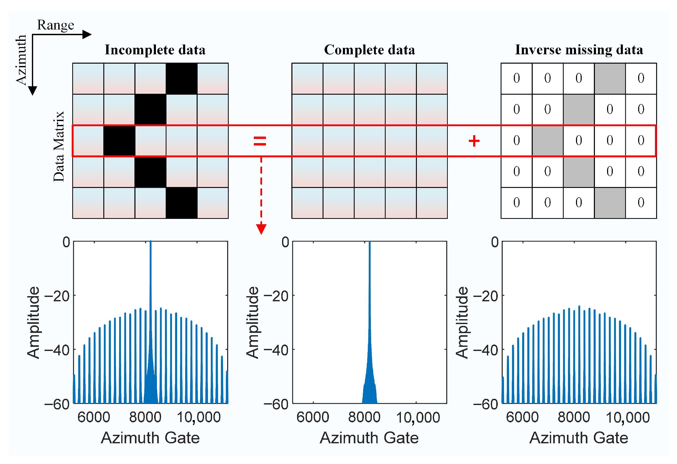
In this approach, the staggered SAR signal can be modeled as the superposition of two parts, including the complete data and the negative counterpart of the missing data, hereafter referred to as the inverse missing data. These inverse components are the primary contributors to artifact generation, as illustrated in Figure 3. Accordingly, filtering out this component would allow recovery of the complete data. However, directly filtering it in the time domain is impractical since the inverse missing data partially cancels with the blind range, making separation difficult. In the frequency domain, both components share the same Doppler bandwidth, further complicating filtering. Therefore, alternative approaches must be considered in other domains to address this issue effectively.

Figure 3. Schematic of (top) incomplete data and (bottom) corresponding 1-D azimuth compression result, where artifacts are attributed to inverse missing data, assuming nonuniformity correction.

Fortunately, the distribution characteristics of artifacts in staggered SAR, derived from (8), reveal that except for the zero-order ($n=0$) artifact, the remaining artifacts are equally spaced at distinct positions relative to the main image, exhibiting spatial separability. This property provides a novel approach for subsequent processing. By isolating these artifacts from the main image using a spatial domain filter and applying inverse-matched filtering, ABIF effectively filters out the inverse component and reconstructs the complete signal. The necessity of ABIF arises from two main points. First, the assumption behind CGPE breaks down when the signal phase does not satisfy local linear characteristics, which is often difficult to achieve in real scenarios. Second, the regular distribution characteristics of artifacts provide an opportunity to separate artifacts from the main image in the spatial domain, thereby enabling the approximation of inverse missing data filtering and ultimately completing data recovery.

Assume that the azimuth compression result is divided into multiple subblocks through a spatial domain filter. Each subblock excludes the first- and higher-order artifacts generated by the inverse missing data in the current subblock. Assume that there are P targets within the kth subblock, then we obtain

$$\begin{array}{cc}\hfill & {\mathrm{y}}_k\left(\eta \right)=w_k\left(\eta \right)·\sum _{i=1}^P{y}_{\mathrm{non},\mathrm{m},i}\left(\eta \right)\hfill \\ \hfill & =w_k\left(\eta \right)·\sum _{i=1}^P{\sigma }_i·E_{\mathrm{c}}\left\{\sum _{n=-N/2}^{N/2-1}{C}_{n,i}\mathrm{sinc}\left[\left(\eta -{\displaystyle \frac{n{f}_{\mathrm{s}}}{K_{\mathrm{a}}}}\right)B_{\mathrm{a}}\right]\right\}\hfill \\ \hfill & \approx \sum _{i=1}^P{\sigma }_i·E_{\mathrm{c}}\left\{C_{0,i}\mathrm{sinc}\left[\eta B_{\mathrm{a}}\right]\right\}+n_{\mathrm{a}}\left(\eta \right).\hfill \end{array}$$

(10)

Among them, $w_k\left(\eta \right)$ is the azimuth spatial domain filter window, which is essentially a time-domain truncation function varying with slow time. $y_{\mathrm{non},\mathrm{m},i}\left(\eta \right)$ is the matched filtering result of ith target. $E_{\mathrm{c}}=exp\left(-j4\pi R_0/\phantom{4\pi R_0\lambda }\lambda \right)exp\left(j2\pi f_{{\eta }_{\mathrm{c}}}\eta \right)$, $C_{n,i}=E_{n,i}{B}_{\mathrm{a}}\left(M_{n,i}+b_{n,i}\right)$, where the subscript i denotes the coefficient corresponding to the ith target. $n_{\mathrm{a}}\left(\eta \right)$ is the artifact energy from other subblocks superimposed onto the processed subblock, and its value is relatively small. Then, the azimuth subblock signal ${\mathrm{y}}_k\left(\eta \right)$ is inverse matched filtered to obtain $s_{\mathrm{inv},k}\left(\eta \right)$, that is

$$\begin{array}{cc}\hfill s_{\mathrm{inv},k}\left(\eta \right)& ={\mathrm{y}}_k\left(\eta \right)\otimes h^{*}\left(\eta \right)\hfill \\ \hfill & ={\widehat{E}}_{\mathrm{c}}·\sum _{i=1}^P{\sigma }_i·{\widehat{C}}_{0,i}\mathrm{rect}\left[{\displaystyle \frac{\eta -{\eta }_{c,i}}{T_{\mathrm{a}}}}\right]+n_{\mathrm{a}}\left(\eta \right)\hfill \\ \hfill & \approx {\widehat{E}}_{\mathrm{c}}·\sum _{i=1}^P{\sigma }_i·\mathrm{rect}\left[{\displaystyle \frac{\eta -{\eta }_{c,i}}{T_{\mathrm{a}}}}\right]\hfill \\ \hfill & =s_{\mathrm{ori},k}\left(\eta \right)\hfill \end{array}$$

(11)

where $h\left(\eta \right)$ is the matched filter in the time domain, the symbol ∗ denotes the conjugate, and $s_{\mathrm{ori},k}\left(\eta \right)$ is the original signal without data gaps. ${\widehat{E}}_{\mathrm{c}}=exp\left(-j4\pi R_0/\phantom{4\pi R_0\lambda }\lambda \right)exp\left(-j\pi K_{\mathrm{a}}{\eta }^2\right)$, ${\widehat{C}}_{0,i}=M_{0,i}+b_{0,i}$.

At this time, the decompressed signal $s_{\mathrm{inv},k}\left(\eta \right)$ no longer contains inverse missing data. However, artifacts caused by data nonuniform overlap with those induced by inverse missing data, so the outcome can only approximate the ideal case of perfect removal. Nevertheless, back-propagating the decompressed signal to the missing positions enables an effective approximated data recovery from an alternative perspective.

3. Proposed Method

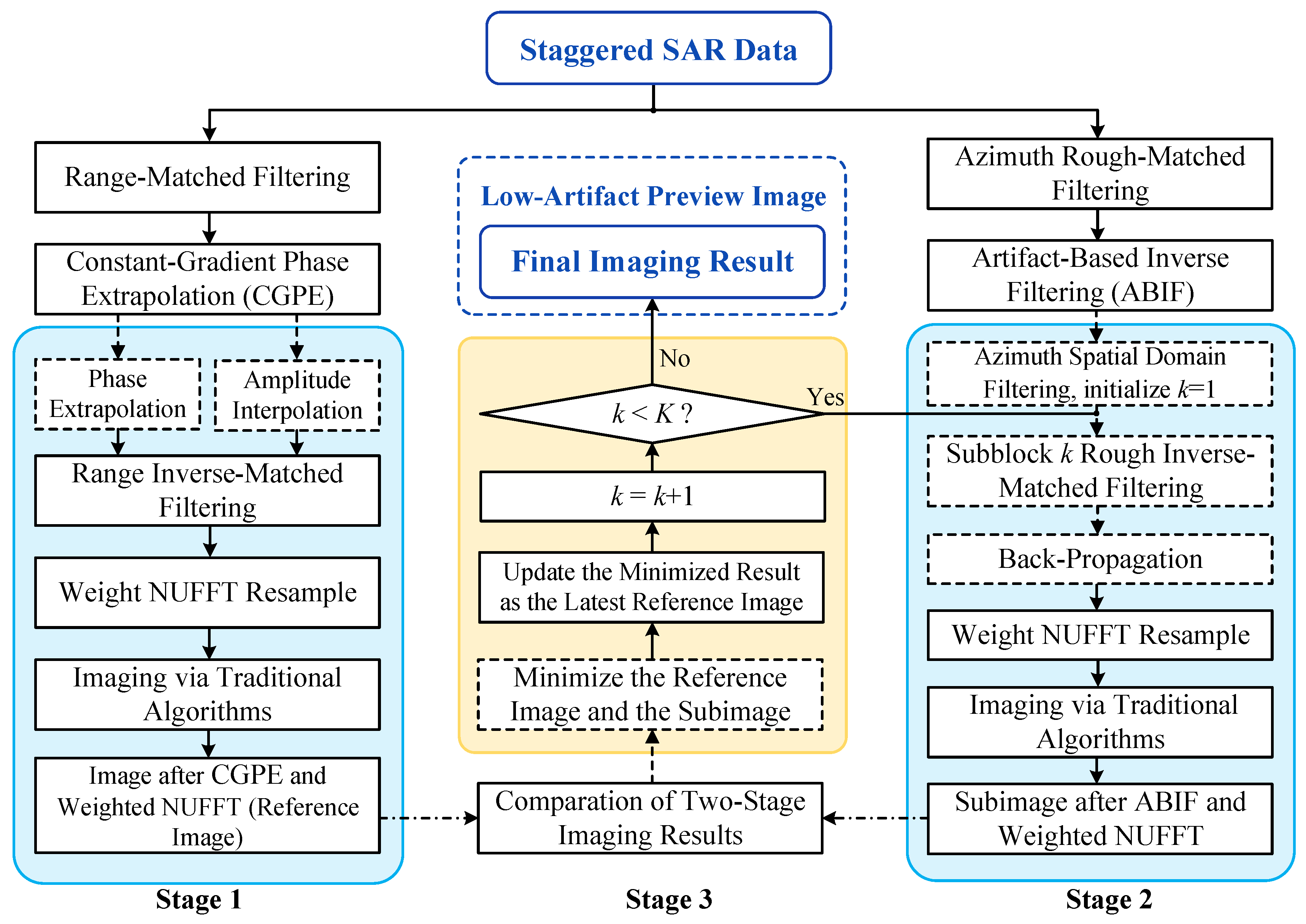
This section presents a low-artifact preview image generation method based on a three-stage processing framework. The first two stages perform data recovery, resampling, and conventional imaging operations to produce intermediate images. The final stage fuses the outputs of the previous stages to generate a complete image with significantly reduced artifacts or nearly artifact-free quality.

3.1. Stage 1: Imaging Based on CGPE and Weighted NUFFT

The first stage is an imaging operation based on CGPE and weighted NUFFT. This processing effectively suppresses high-intensity artifacts generated by targets with locally linear phase characteristics, making it particularly suitable for isolated strong point-like targets in high-contrast scenes. Moreover, it reduces the distribution range of artifacts arising from other types of targets, thereby facilitating subsequent processing.

Firstly, data recovery is completed via CGPE, and the recovered data after CGPE is denoted as $s_{\mathrm{CGPE}}\left(\eta \right)$. Specifically, the phase and amplitude estimation of the signal at the missing position are

$$\begin{array}{cc}\hfill \theta \left({\eta }_{\mathrm{int}}\right)=& {\displaystyle \frac{\theta \left[{\eta }_{\mathrm{int}}-\Delta {\eta }_a\right]-\theta \left[{\eta }_{\mathrm{int}}-\Delta {\eta }_{a-1}\right]}{\Delta {\eta }_a-\Delta {\eta }_{a-1}}}·\Delta {\eta }_a\hfill \\ \hfill & +\theta \left[{\eta }_{\mathrm{int}}-\Delta {\eta }_a\right]\hfill \end{array}$$

(12)

$$\begin{array}{cc}\hfill A\left({\eta }_{\mathrm{int}}\right)=& {\displaystyle \frac{A\left[{\eta }_{\mathrm{int}}+\Delta {\eta }_{a+1}\right]-A\left[{\eta }_{\mathrm{int}}-\Delta {\eta }_a\right]}{\Delta {\eta }_{a+1}+\Delta {\eta }_a}}·\Delta {\eta }_a\hfill \\ \hfill & +A\left[{\eta }_{\mathrm{int}}-\Delta {\eta }_a\right]\hfill \end{array}$$

(13)

where ${\eta }_{\mathrm{int}}$ is the slow time corresponding to the missing position, $\Delta {\eta }_a$ and $\Delta {\eta }_{a-1}$ represent the time intervals between ${\eta }_{\mathrm{int}}$ and its preceding and its two preceding sampling times, respectively. $\Delta {\eta }_{a+1}$ denotes the interval between ${\eta }_{\mathrm{int}}$ and its subsequent sampling time.

However, due to the nonuniform nature of the data, a resampling operation is essential to follow. Azimuth resampling employs the weighted NUFFT method [37]. In contrast to uniform sampling, where energy is distributed uniformly in the time domain, nonuniform sampling exhibits uneven energy distribution. Therefore, the key idea of the weighted NUFFT is to apply weighting to the time-domain signal, where the weighting coefficient for the lth sample is given by

$${\omega }_l={\displaystyle \frac{1}{\mathrm{PR}{\mathrm{I}}_{\mathrm{mean}}}}·\left({\displaystyle \frac{{\eta }_{l+1}-{\eta }_{l-1}}{2}}\right)$$

(14)

where ${\eta }_{l-1}$ and ${\eta }_{l+1}$ are the slow times of the $\left(l-1\right)$th and $\left(l+1\right)$th samples, respectively.

The three classical resampling methods: BLU [18], the primitive NUFFT [38], and the weighted NUFFT [37], are compared, and the compression results after resampling are illustrated in Figure 4. The comparison only evaluates the resampling effects without considering data gaps. By compensating for the energy imbalance caused by nonuniform sampling, the weighted NUFFT achieves superior compression results than the primitive one. Compared to the BLU method, the weighted NUFFT eliminates pairs of high lobes in the azimuth center. Consequently, adopting the weighted NUFFT method is a feasible approach for resampling. Therefore, the imaging result $I_{a,\mathrm{CGPE}}\left(\eta \right)$ after CGPE recovery and weighted NUFFT resampling is

$$I_{\mathrm{a},\mathrm{CGPE}}\left(\eta \right)={{\mathcal{F}}_{\mathrm{a}}}^{-1}\left\{{\mathcal{F}}_{\mathrm{a},\mathrm{wn}}\left[s_{\mathrm{CGPE}}\left(\eta \right)\right]·H_{\mathrm{a}}\left(f_{\eta }\right)\right\}$$

(15)

where ${{\mathcal{F}}_a}^{-1}\left(·\right)$ and ${\mathcal{F}}_{\mathrm{a},\mathrm{wn}}\left(·\right)$ represent the inverse Fourier transform and the weighted nonuniform Fourier transform in azimuth, $H_{\mathrm{a}}\left(f_{\eta }\right)$ corresponds to the matched filter in the azimuth frequency domain.

Figure 4. Comparison of compression results for different resampling methods. From left to right are the results of BLU, the primitive NUFFT, and the weighted NUFFT. The simulation parameter is shown in Table 1.

Figure 4. Comparison of compression results for different resampling methods. From left to right are the results of BLU, the primitive NUFFT, and the weighted NUFFT. The simulation parameter is shown in Table 1.

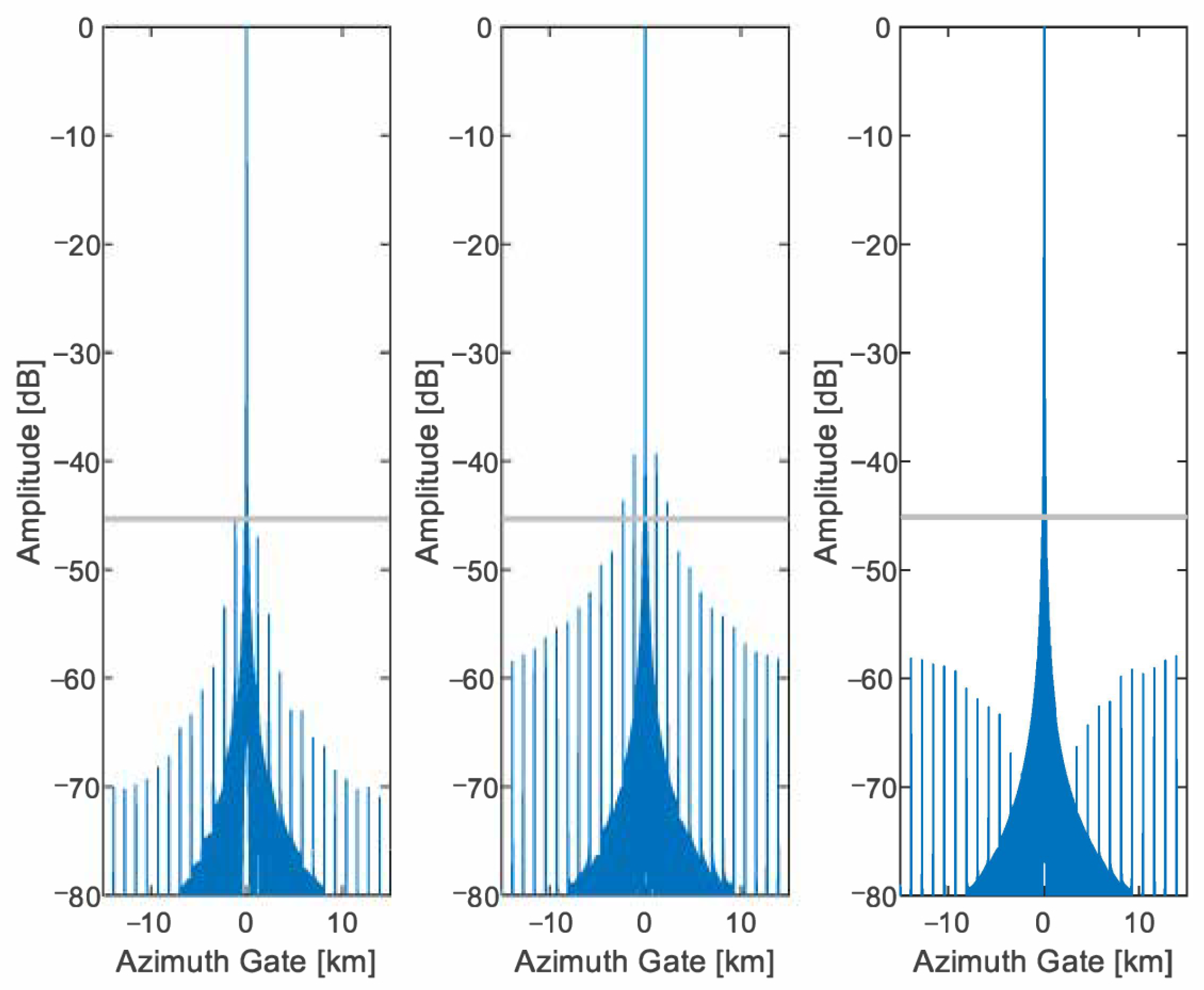
Table 1. System simulation parameters.

Parameter	Value
System Carrier Frequency	1.25 GHz
Orbit Height	760 km
Platform Velocity	7473 m/s
Imaging Slant Range	868∼1097 km
Pulse Duration	20 $\mathsf{\mu }$s
Pulse Bandwidth	60 MHz
Range Sampling Frequency	64 MHz
Processed Doppler Bandwidth	1495 Hz
Mean PRF	1816 Hz

Table 1. System simulation parameters.

Parameter	Value
System Carrier Frequency	1.25 GHz
Orbit Height	760 km
Platform Velocity	7473 m/s
Imaging Slant Range	868∼1097 km
Pulse Duration	20 $\mathsf{\mu }$s
Pulse Bandwidth	60 MHz
Range Sampling Frequency	64 MHz
Processed Doppler Bandwidth	1495 Hz
Mean PRF	1816 Hz

3.2. Stage 2: Imaging Based on ABIF and Weighted NUFFT

The second stage performs imaging based on ABIF and weighted NUFFT, aiming to correct the estimation errors from the first stage. Unlike the first stage, which processes the entire scene, this stage operates an imaging operation on multiple azimuthal subblocks. This approach imposes no assumptions on target characteristics, allowing for more flexible data recovery and robust artifact suppression.

To mitigate estimation errors introduced by CGPE processing, the imaging result of the original missing signal $s_{\mathrm{non},\mathrm{m}}\left(\eta \right)$ is selected as the ABIF object, denoted as $I_{\mathrm{a}}\left(\eta \right)$, which can be obtained by

$$I_{\mathrm{a}}\left(\eta \right)={{\mathcal{F}}_{\mathrm{a}}}^{-1}\left\{{\mathcal{F}}_{\mathrm{a}}\left[s_{\mathrm{non},\mathrm{m}}\left(\eta \right)\right]·H_{\mathrm{a}}\left(f_{\eta }\right)\right\}$$

(16)

where ${\mathcal{F}}_{\mathrm{a}}\left(·\right)$ is the Fourier transform in azimuth. The kth subblock $I_{\mathrm{a},k}\left(\eta \right)$ under the effect of the azimuth spatial domain filter window is obtained by

$$\begin{array}{cc}\hfill I_{\mathrm{a},k}\left(\eta \right)& =w_k\left(\eta \right)·I_{\mathrm{a}}\left(\eta \right)\hfill \\ & =w_{k1}\left(\eta \right)·w_{k2}\left(\eta \right)·I_{\mathrm{a}}\left(\eta \right)\hfill \\ & =w_{k2}\left(\eta \right)·I_{\mathrm{a}}\left[\eta +\left(k-1\right){\Delta }_{\mathrm{s}}\right],\eta \in \left[1,N_{\mathrm{s}}\right]\hfill \\ & =\left\{\begin{array}{c}{I}_{\mathrm{a}}\left[\eta +\left(k-1\right){\Delta }_{\mathrm{s}}+{\displaystyle \frac{{\Delta }_{\mathrm{N}}}{2}}\right],\eta \in \left[1,N_{\mathrm{t}}\right]\hfill \\ 0,\mathrm{otherwise}\hfill \end{array}\right.\hfill \end{array}$$

(17)

where $k=1,2,\dots ,K$ and K is the number of subblocks, $N_{\mathrm{s}}$ is the subblock size, $N_{\mathrm{t}}$ is the retained sample size of each subblock, ${\Delta }_{\mathrm{s}}$ denotes the step size of the subblock, ${\Delta }_{\mathrm{N}}=N_{\mathrm{s}}-N_{\mathrm{t}}$.

Firstly, the selection of $N_{\mathrm{s}}$ is critical, and it must exceed the artifact span of the target following the first stage. The $N_{\mathrm{t}}$ should be less than $\Delta =f_{\mathrm{s}}/\phantom{f_{\mathrm{s}}\left(K_{\mathrm{a}}·\mathrm{PR}{\mathrm{I}}_{\mathrm{mean}}\right)}\left(K_{\mathrm{a}}·\mathrm{PR}{\mathrm{I}}_{\mathrm{mean}}\right)$, which prevents the inclusion of artifacts from the target in the retained samples of the current subblock. Additionally, $N_{\mathrm{t}}$ should exceed the 3 dB width of a target to ensure comprehensive information capture. Ideally, a smaller $N_{\mathrm{t}}$ minimizes the energy of artifacts from targets within adjacent subblocks, although it increases the computational burden. Furthermore, ${\Delta }_{\mathrm{s}}$ should be slightly smaller than $N_{\mathrm{t}}$.

Then, the inverse-matched filtering is applied to $I_{\mathrm{a},k}\left(\eta \right)$ in turn. The decompressed signal of subblock k is obtained by

$$s_{\mathrm{d},k}\left(\eta \right)={{\mathcal{F}}_{\mathrm{a}}}^{-1}\left\{{\mathcal{F}}_{\mathrm{a}}\left[I_{\mathrm{a},k}\left(\eta \right)\right]·{H_{\mathrm{a},\mathrm{sub}}}^{-1}\left(f_{\eta }\right)\right\}$$

(18)

where $H_{\mathrm{a},\mathrm{sub}}^{-1}\left(f_{\eta }\right)$ is the azimuth inverse matched filter of the subblock signal.

Furthermore, original data missing causes energy dispersion into artifacts, thus leading to energy loss in the decompressed signal. To compensate for this, $s_{\mathrm{d},k}\left(\eta \right)$ must be multiplied by a coefficient $\beta =M/\phantom{M{M}_{\mathrm{e}}}{M}_{\mathrm{e}}$, where $M_{\mathrm{e}}$ is the number of non-missing samples in a PRI period. In addition, the decompressed signal will exhibit Gibbs effects due to the truncation of the time-domain impulse response. This effect becomes more pronounced as $N_{\mathrm{t}}$ decreases and can be mitigated by incorporating smoothing windows.

At this point, the decompressed signal for each subblock no longer contains gaps at the originally missing positions. This enables back-propagation of the decompressed signal values to those positions, thereby completing the data recovery process. The recovered data for subblock k is given by

$$s_{\mathrm{re},k}\left(\eta \right)=w_{k1}\left(\eta \right)·s_{\mathrm{non},\mathrm{m}}\left(\eta \right)+\beta ·s_{\mathrm{d},k}\left(\eta \right)·{\tilde{B}}_k\left(\eta \right).$$

(19)

Among them, ${\tilde{B}}_k\left(\eta \right)=w_{k1}\left(\eta \right)·\left[1-B\left(\eta \right)\right]$, where $B\left(\eta \right)$ represents a 1-D missing vector derived from a two-dimensional (2-D) missing matrix. The elements of 0 or 1 indicate the presence or absence of data gaps, respectively.

Next, data resampling is also performed using the weighted NUFFT. Therefore, the imaging result of the subblock k after the second stage is

$$I_{\mathrm{re},k}\left(\eta \right)={{\mathcal{F}}_{\mathrm{a}}}^{-1}\left\{{\mathcal{F}}_{\mathrm{a},\mathrm{wn}}\left[s_{\mathrm{re},k}\left(\eta \right)\right]·H_{\mathrm{a},\mathrm{sub}}\left(f_{\eta }\right)\right\}$$

(20)

where $H_{\mathrm{a},\mathrm{sub}}\left(f_{\eta }\right)$ corresponds to the azimuth matched filter of the subblock signal.

3.3. Stage 3: Fusion of Two-Stage Images

At this stage, the processed images from the first two stages have been obtained. However, the image from the first stage can only suppress artifacts caused by isolated strong point-like targets, while each subimage from the second stage is limited to mitigating artifacts within its corresponding subblock. Therefore, a final fusion of these images is required to achieve comprehensive artifact suppression across the entire scene.

The fusion process operates on two levels: between the images from the first and second stages and among the subimages within the second stage. Specifically, the image from the first stage serves as the initial reference. For each subimage, the pixel-wise minimum amplitude between the subimage and the current reference is selected to update the reference image. This process is repeated until all subimages have been fused. In this way, artifacts present in the current subimage are suppressed without reintroducing those removed by previously fused subimages. Furthermore, this strategy ensures that the final image quality is no worse than that of the initial reference image. The complementary strengths of the first two stages, combined with the image fusion in the final stage, collectively enable effective and efficient artifact suppression across the entire scene.

3.4. Implementation Process of 2-D Case

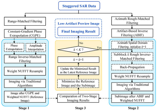
Previously, the 1-D situation has been discussed. Now, we extend the discussion to the 2-D case, with the overall processing flow illustrated in Figure 5. Firstly, the CGPE is performed after range-matched filtering to improve the range signal-to-noise ratio. However, this operation increases the extent of the blind range. Each blind range is extended by half a pulse width outward to acquire the new distribution. The new blind range includes incompletely compressed regions, which have a small impact on azimuth phase estimation but a significant effect on amplitude estimate. To mitigate this, the bilateral averaging used for amplitude recovery at missing positions can, if necessary, be simplified to a unilateral approach, thereby avoiding reliance on incomplete data. In addition, ABIF does not need to be performed in the 2-D image domain. It only requires transformation into the azimuth image domain via direct azimuth-matched filtering. As no operations are conducted in the range dimension, this process is referred to as azimuth rough-matched filtering. The subsequent steps, consistent with those described in the 1-D case, are omitted here for brevity.

Figure 5. Flowchart of proposed method for staggered SAR data.

Finally, it is important to emphasize the indispensable roles of the first two stages, which constitute the core foundation of the proposed method. The first stage effectively suppresses artifacts induced by isolated strong point-like targets that severely degrade image quality. The second stage, operating without any assumptions on target characteristics, is capable of mitigating artifacts generated by various types of scatterers. However, relying on the second stage alone is insufficient, as the subblock size $N_{\mathrm{s}}$ must exceed the spatial extent of the artifacts to achieve effective suppression. In this regard, the preceding CGPE step reduces the extent of artifact, thereby allowing the use of smaller subblocks and improving overall processing efficiency.

4. Experimental Results

In this section, a series of simulations for point and distributed targets are conducted to verify the efficiency of the proposed method. The experiments are implemented using MATLAB R2025a on a computer with a 16-core 2.4 GHz CPU and 64 GB of memory.

4.1. Point Target Simulation

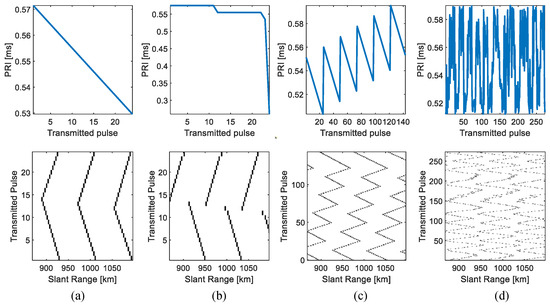
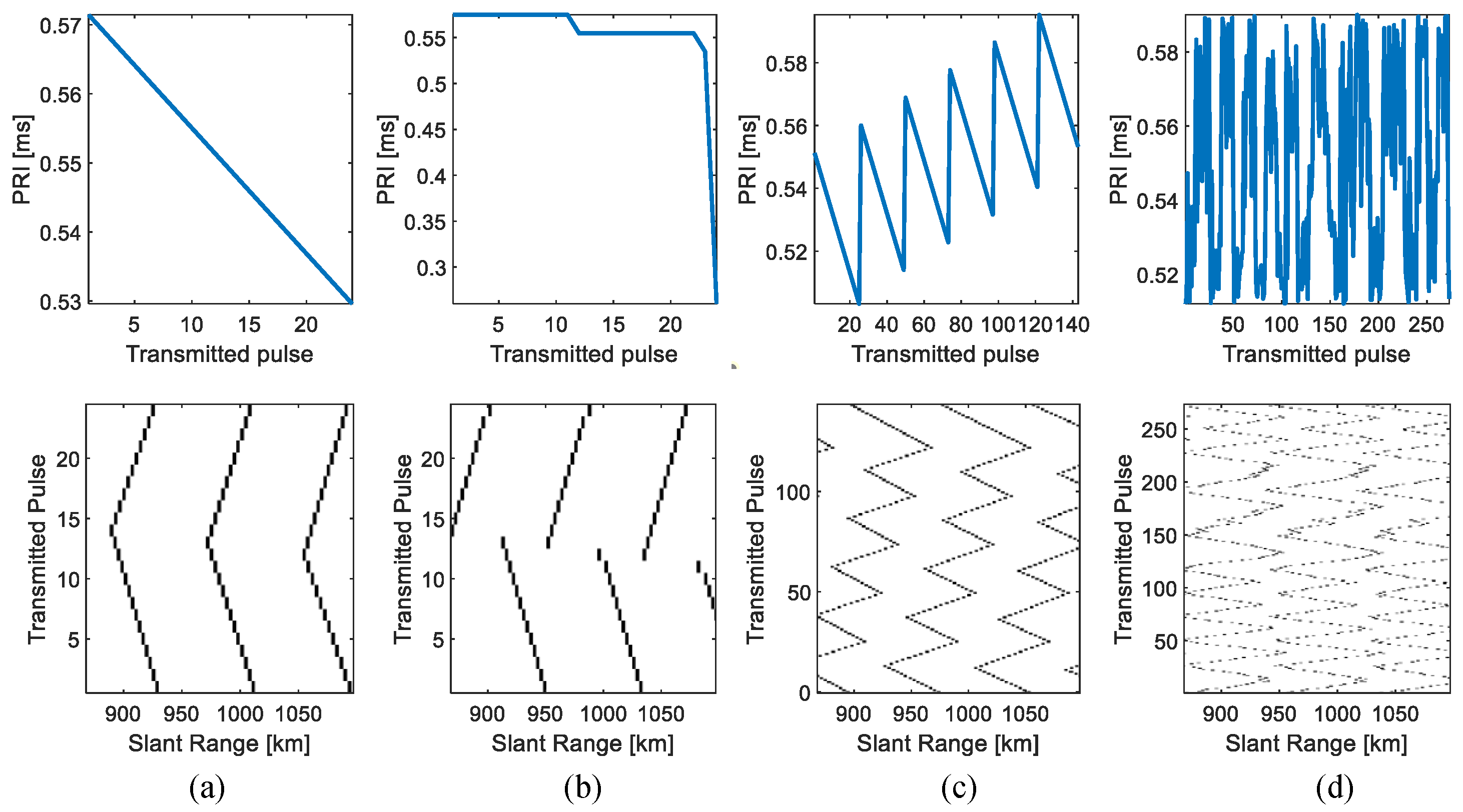
In this subsection, simulations for point targets are conducted using the parameters listed in Table 1. Four types of PRI sequences are considered: fast PRI variation [18], stepped PRI variation [30], elaborated PRI variation [18], and nonlinear PRI variation [33]. Among them, the fast and stepped PRI variations are categorized as short-period sequences due to smaller periods, while elaborated and nonlinear PRI variations are classified as long-period sequences. All sequences maintain an average PRF of approximately 1816 Hz, corresponding to the same azimuth oversampling ratio. Further details about PRIs are provided in Figure 6.

Figure 6. Illustration of the different PRI sequences used in the simulations. From left to right are the PRI values within one period and the blind range distribution. (a) Fast PRI variation ($\mathrm{PR}{\mathrm{I}}_1=0.571\mathrm{ms},\mathrm{M}=24$). (b) Stepped PRI variation ($\mathrm{PR}{\mathrm{I}}_1=0.574\mathrm{ms},\mathrm{M}=24$). (c) Elaborated PRI variation ($S=6,\mathrm{PR}{\mathrm{I}}_1\left(S\right)=0.595\mathrm{ms},\mathrm{M}=143$). (d) Nonlinear PRI variation ($\mathrm{PR}{\mathrm{I}}_{max}=0.590\mathrm{ms},\mathrm{PR}{\mathrm{I}}_{min}=0.512\mathrm{ms},\mathrm{M}=273$).

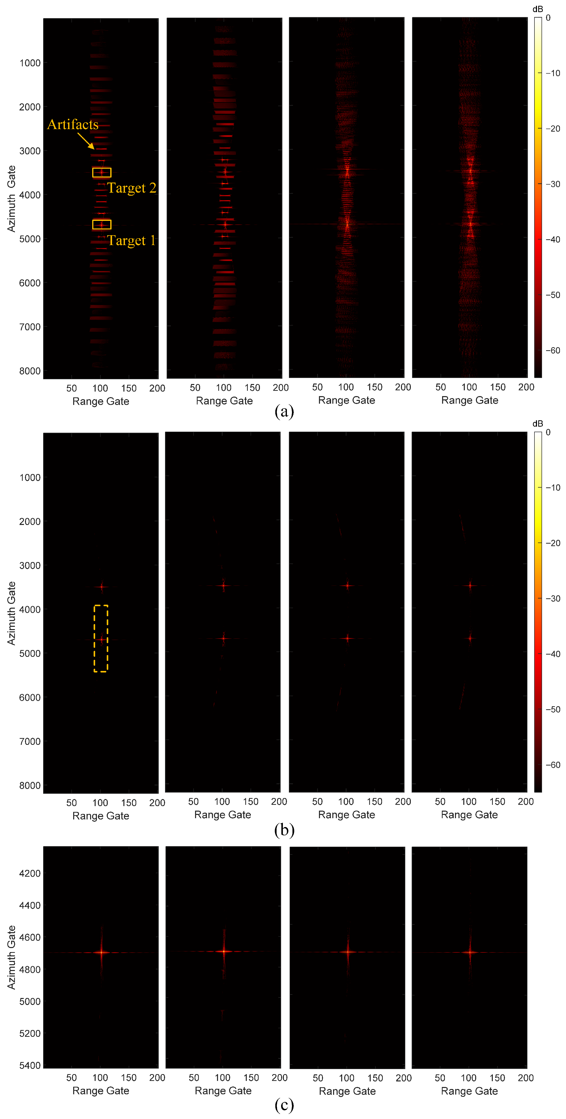
Now, 2-D simulation is conducted to demonstrate the effectiveness of the proposed method for different types of PRIs. The simulation involves two targets at the same slant range but with different azimuth positions, separated by 1200 samples. The reason for not using a single point target in the simulation is that such a target fully satisfies the local phase linearity, allowing perfect recovery with only the first stage processing. As a result, the effectiveness of the proposed method cannot be demonstrated.

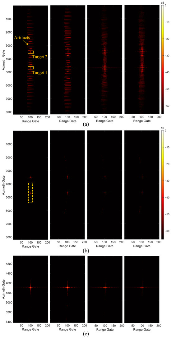
The imaging results are shown in Figure 7, and from left to right, are the results under fast, stepped, elaborated, and nonlinear PRI variation sequences. The direct imaging result is shown in Figure 7a. Specifically, the average PRI is obtained by calculating the average value of the employed PRI sequence first. Based on this average PRI, conventional SAR imaging methods, such as the chirp scaling algorithm (CSA), are then applied to the raw data to obtain the direct imaging results. For short-period sequences, adjacent artifacts are farther apart, yet the intensity of individual artifacts remains high. Conversely, for long-period sequences, artifact energy is dispersed over the entire synthetic aperture time. Except for the first few order artifacts, which are higher due to strong nonuniformity, the intensity of the remaining individual artifacts has decreased.

Figure 7. 2-D staggered SAR imaging results using fast, stepped, elaborated, and nonlinear PRI variation sequences (from left to right). (a) Direct imaging via CSA. (b) Imaging results after the proposed method. (c) Zoom-in on Target 1 (yellow dashed box in (b)).

After adopting the proposed method, the high-intensity artifacts around the target almost disappear, as shown in Figure 7b. The parameters of the proposed method are set as $N_{\mathrm{s}}=6500$, $N_{\mathrm{t}}=140$, ${\Delta }_{\mathrm{s}}=120$. Notably, under long-period PRI sequences, the subblock sample size $N_{\mathrm{t}}$ used for ABIF remains consistent with that used in short-period cases. To better visualize the artifact suppression performance, a magnified view of Target 1 is provided in Figure 7c. The simulation scene consists of 8192 × 8192 samples (azimuth × range), and the total running time of the proposed method is approximately 2 min for all PRI sequences. As a result, the proposed method demonstrates good performance under various PRI strategies, significantly suppressing artifacts with a short execution time.

4.2. Distributed Target Simulation

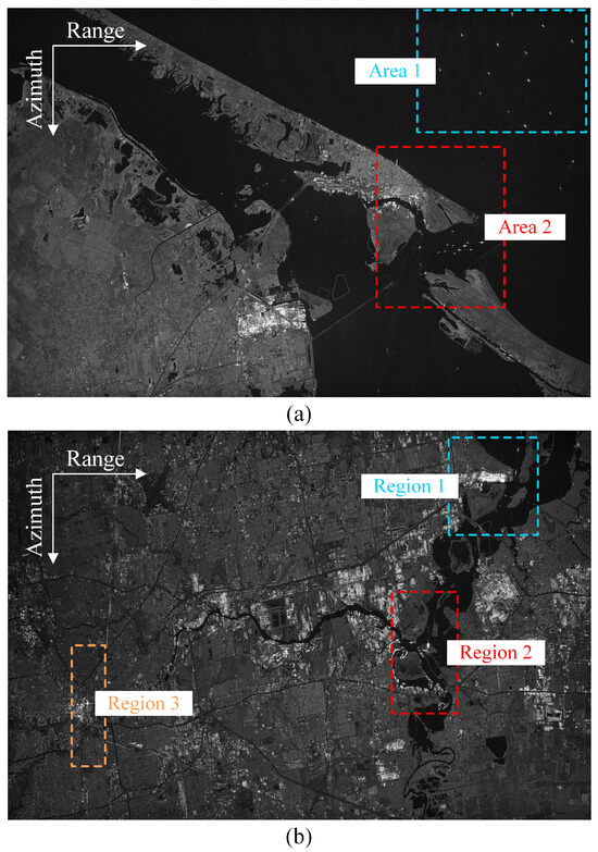
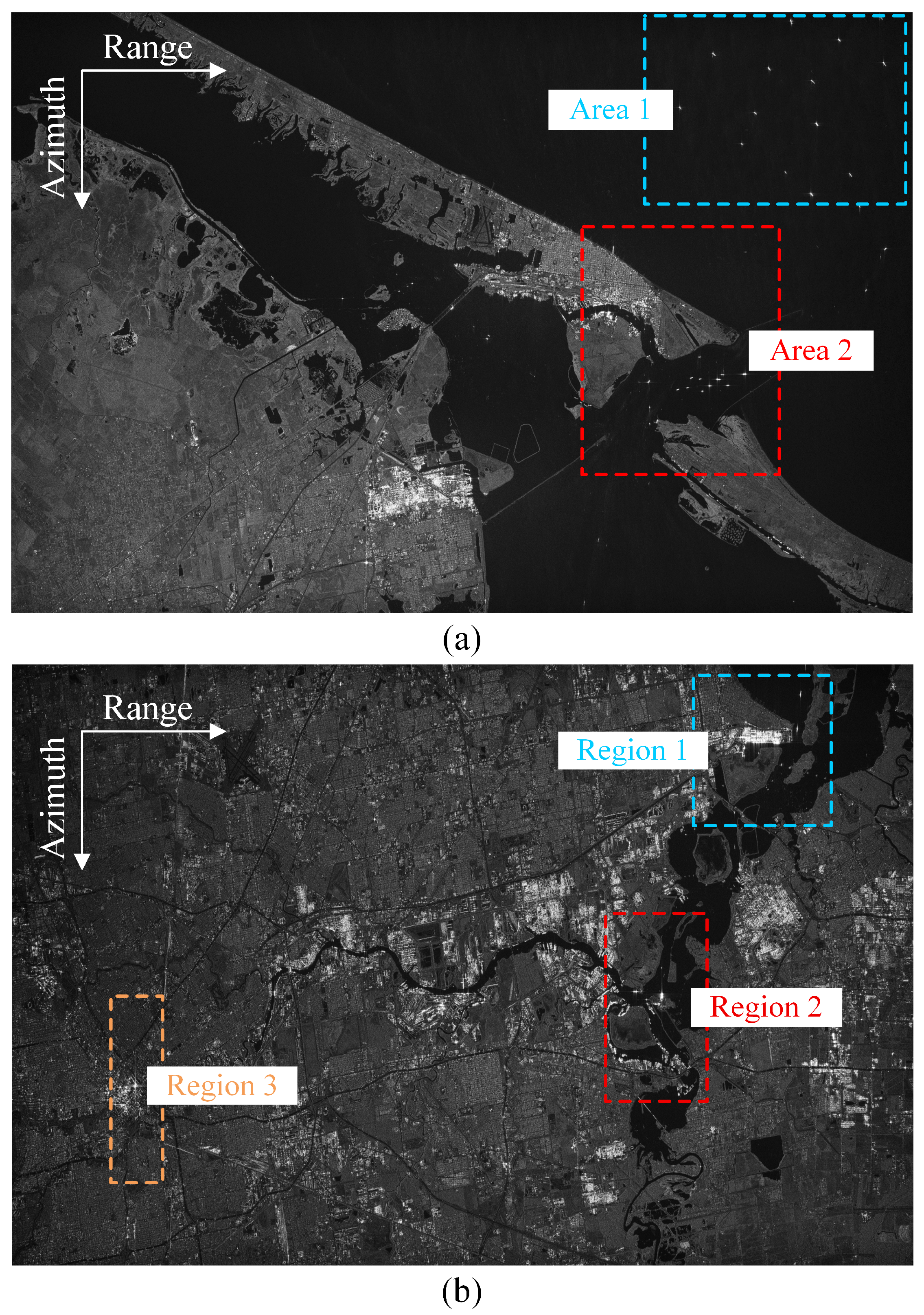
In this subsection, spaceborne SAR data is employed to verify the feasibility of the proposed method for distributed targets. Sentinel-1 raw data (stripmap mode), acquired in the Houston Bay area, is selected as the experimental data. The imaged scene covers an area of approximately 30 km × 35 km (azimuth × range). The image of Sentinel-1 raw data is used as the reference image and acts as the baseline for comparison, as shown in Figure 8. To simulate staggered SAR data, the raw signal is resampled based on various PRIs with corresponding blind ranges set. All subsequent processing is performed on this equivalent dataset. The parameters of the proposed method are set as $N_{\mathrm{s}}=2048$, $N_{\mathrm{t}}=120$, ${\Delta }_{\mathrm{s}}=80$.

Figure 8. (a) Reference image of the distributed targets in sea areas. (b) Reference image of the distributed targets in complex urban areas. The dotted boxes in the figure indicate several areas containing strong-scattering targets.

First, a scene with a relatively clean background is selected, as shown in Figure 8a. The analysis focuses on the two areas indicated by the dashed boxes. Specifically, Area 1 is relatively simple and contains only ships, while Area 2 is more complex, including sea surface, islands, and other features.

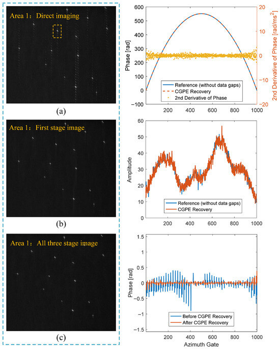
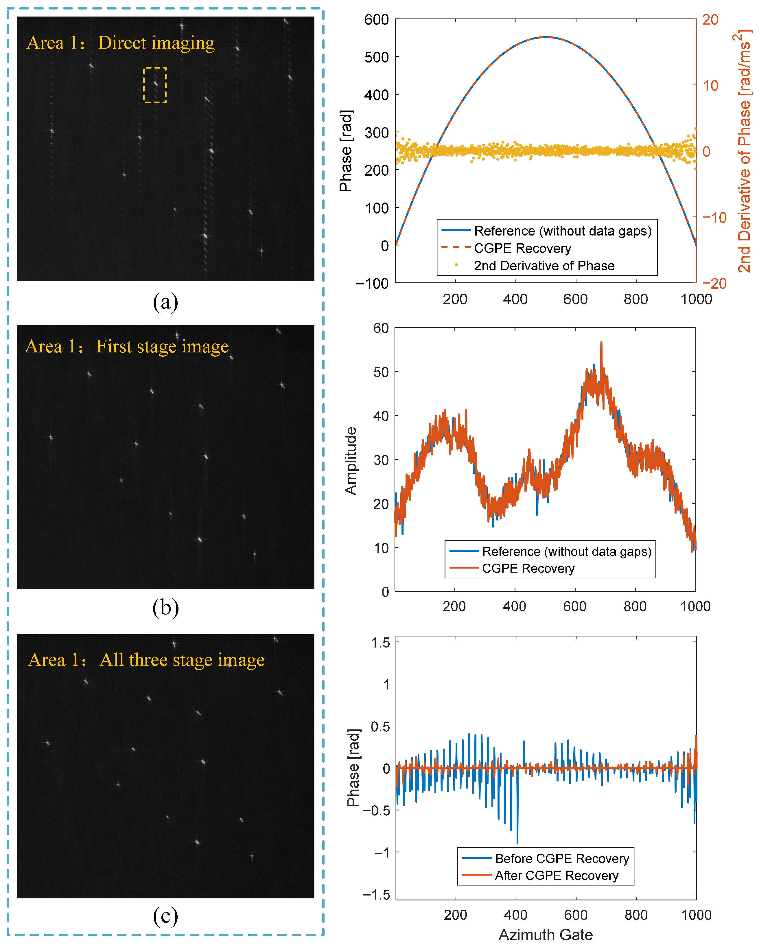
In Figure 9, the imaging results of Area 1 under the equivalent staggered SAR system parameters are presented, with the data resampled according to fast PRI variation sequence ($\mathrm{PR}{\mathrm{I}}_1=0.746\mathrm{ms},\mathrm{M}=18$). From top to bottom, the images show the direct imaging result, the first-stage image, and the result using the complete method. The weak sea surface background and independently strong point-like targets, such as ships in Area 1, cause the signal phase to exhibit local linear characteristics. On the right side of Figure 9, the phase and amplitude of the target enclosed by the dashed box in Figure 9a are displayed from top to bottom, along with the phase error before and after CGPE processing. The second derivative of the signal phase is observed to be approximately zero, confirming the validity of the local linear phase assumption. In addition, the amplitude variation between adjacent samples is minimal, indicating that bilateral averaging does not significantly distort the amplitude characteristics. Thus, the high artifacts near the ship targets after applying CGPE are almost suppressed, with only a small amount of artifact energy remaining. Moreover, the running time is very short. Following the application of ABIF and image fusion in the final stage, the artifacts in Area 1 are effectively eliminated, yielding a clean imaging result.

Figure 9. Imaging results of Area 1, where (a) is the direct imaging result, (b) is the first-stage image, and (c) is the result using the complete method. On the right side of the figure, from top to bottom, are the phase and amplitude of the target enclosed by the dashed box in (a), along with the phase error before and after CGPE processing.

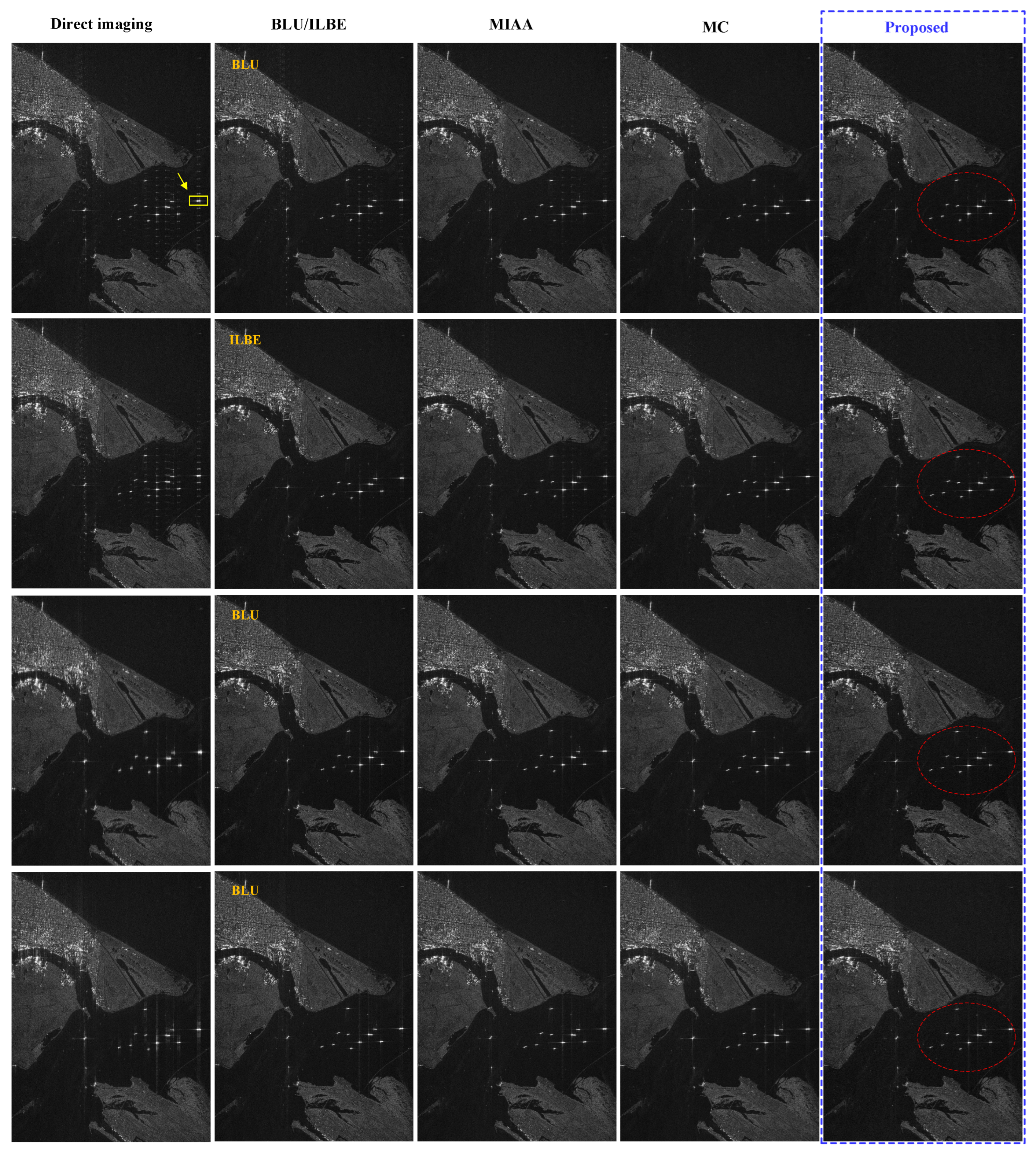
Additionally, further comparative simulations are conducted to evaluate the artifact suppression performance of the proposed method across different PRI sequences. As in the point target simulations, the average PRF is maintained consistently across all types of PRI sequences. The results for Area 2 are shown in Figure 10. From top to bottom, the images correspond to fast, stepped, elaborated, and nonlinear PRI variation sequences. From left to right, the columns display the imaging results obtained using CSA, BLU/ILBE [18,30], MIAA [26], MC [31], and the proposed method, respectively. In the BLU method, BLU is first applied for data recovery and then used for resampling to mitigate performance degradation caused by data gaps. For the case of stepped PRI variation, comparisons are made with the ILBE method [30], an enhancement of the BLU method, which is specifically designed to address the blind range distribution characteristic of stepped PRI variation.

Figure 10. Magnified images of imaging results for Area 2. From top to bottom, the images correspond to fast, stepped, elaborated, and nonlinear PRI variation sequences. Different columns show the results of different methods, as shown at the top of the figure.

The artifact intensity is reduced to varying degrees after BLU processing, when, in the case of fast PRI variation, suppression is limited due to the high energy concentrated in individual artifacts. In contrast, for long-period PRI sequences, artifacts become more dispersed, and BLU can effectively eliminate most of their energy. The ILBE method performs comparatively well for stepped PRI variation, leaving only minimal residual artifact energy. The MIAA and MC methods achieve better artifact suppression but at the expense of significantly longer computation times. In comparison, the proposed method effectively suppresses artifacts within a relatively short running time and maintains acceptable imaging quality across various PRI types. It is worth noting that for long-period PRI sequences, the proposed method cannot eliminate the energy of the first few orders of artifacts fully during ABIF processing, resulting in some residual artifacts. Nevertheless, it still outperforms fast methods like BLU in terms of imaging quality, while offering a substantial reduction in computational time compared to high-precision but computationally intensive methods such as MIAA.

To quantitatively assess the effectiveness of artifact suppression, the azimuth ambiguity-to-signal ratio (AASR) for each method is calculated, as shown in Table 2. To ensure accurate AASR evaluation, we selected a strong scatterer located in a clean background region for the calculation, specifically the ship target indicated by the yellow arrow in Figure 10. In addition, the total running time required to process the entire scene is listed to provide a fair evaluation of computational efficiency. Among these methods, the proposed method demonstrates a lower AASR and relatively short running time. These results indicate that the proposed method not only offers robust imaging performance under various PRI configurations but also enables the generation of preview images within a short time, thereby satisfying the practical requirements for rapid scene interpretation and target screening.

Table 2. Comparison of AASR and running times of different methods under different PRI sequence settings.

PRI Type	Method	AASR [dB]	Running Time [min]
	Direct imaging via CSA	−15.58	0.06
	BLU	−20.95	1.28
Fast PRI Variation	MIAA	−24.45	158.28
	MC	−28.24	131.25
	Proposed method	−29.81	2.79
	Direct imaging via CSA	−13.06	0.06
	ILBE	−24.92	83.18
Stepped PRI Variation	MIAA	−23.98	158.75
	MC	−26.36	140.85
	Proposed method	−27.96	2.98
	Direct imaging via CSA	−15.39	0.07
	BLU	−25.53	1.39
Elaborated PRI Variation	MIAA	−27.75	163.02
	MC	−27.76	128.73
	Proposed method	−27.13	3.07
	Direct imaging via CSA	−14.97	0.06
	BLU	−23.14	1.47
Nonlinear PRI Variation	MIAA	−23.68	162.85
	MC	−24.15	141.78
	Proposed method	−24.10	3.12

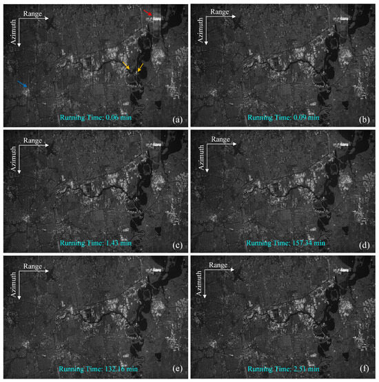
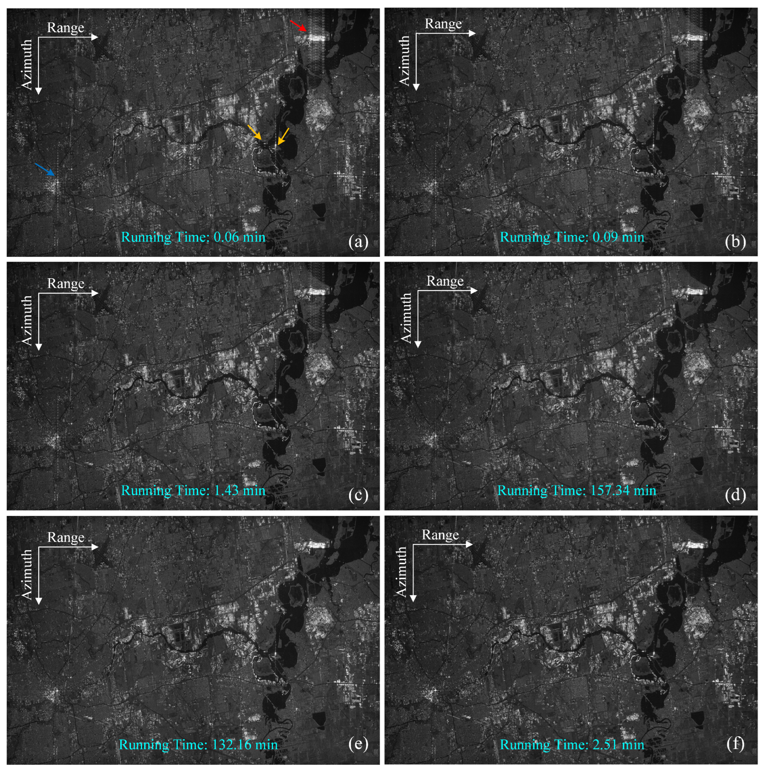
Furthermore, a scene featuring densely urban areas with numerous strong point-like targets is selected for simulation, as shown in Figure 8b. The data is resampled using a fast PRI variation sequence, consistent with the PRI setting used in the previous sea areas. The imaging result obtained directly using CSA is shown in Figure 11a, where the influence of strong point-like targets is visible, especially in Regions 1, 2, and 3. The artifacts generated by such targets are more pronounced in low-intensity background areas, where they are easily observable. In contrast, uniformly distributed targets with low backscattering coefficients, such as farmland and water surfaces, have a much less noticeable impact on the image. The imaging results of two-point linear interpolation [18], BLU, MIAA, MC, and the proposed method are shown in Figure 11b–f, respectively. In addition, the running time for each method is listed below the corresponding image. For the linear interpolation, MATLAB’s built-in function interp1 was used to ensure a standard and efficient implementation.

Figure 11. Large-scale distributed target simulation results of staggered SAR in urban areas. (a) Direct imaging by CSA. (b) Two-point linear interpolation method. (c) BLU method. (d) MIAA method. (e) MC method. (f) Proposed method.

Among the evaluated methods, two-point linear interpolation yields the shortest running time but delivers the poorest imaging performance, with prominent artifacts remaining. The BLU method offers improved image quality compared to interpolation, notably reducing artifacts around Region 1 and the left side of Region 2. However, limited data oversampling prevents complete suppression, and the image quality still falls short of the reference. The MIAA and MC methods further enhance imaging quality by effectively mitigating artifacts in all three regions, albeit at the cost of increased running time. In contrast, the proposed method achieves high-quality imaging across all three regions with a running time of approximately 3 min, significantly faster than both the MIAA and MC methods.

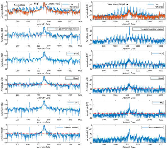
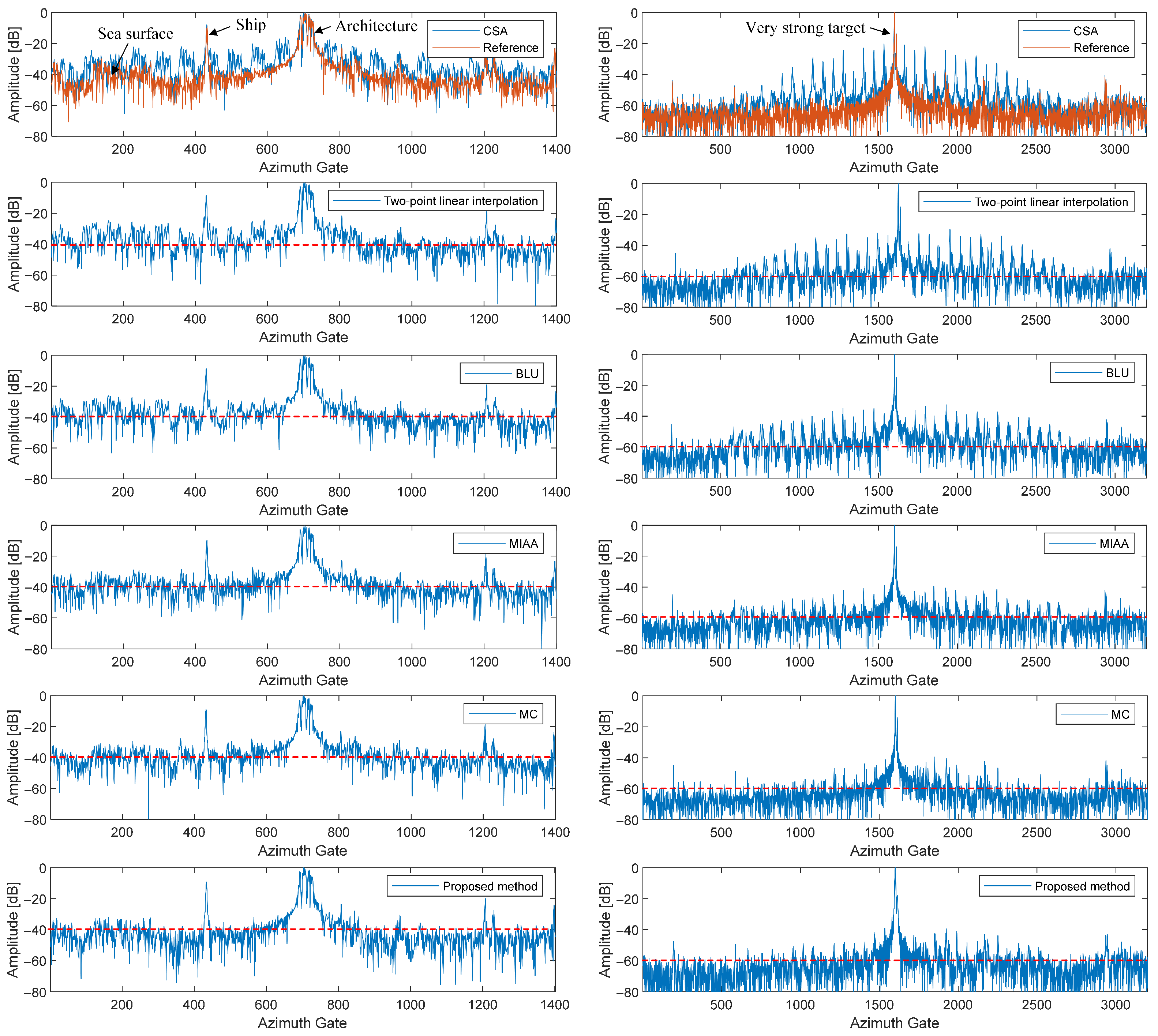
To enable a more detailed comparison, azimuth profiles of strong point-like targets on the right side of Region 2 and Region 3 are analyzed, as shown in Figure 12. The first row compares the reference image with the azimuth profile obtained from direct imaging, revealing that the artifact intensity is significantly higher than that of surrounding targets. The artifact levels are slightly reduced when using two-point linear interpolation and the BLU method. In contrast, the proposed method achieves artifact suppression comparable to that of the MIAA and MC methods while requiring substantially less time. These results indicate that the proposed method enables the efficient generation of staggered SAR preview images, even for complex scenes, while achieving substantial artifact suppression.

Figure 12. Azimuth profile analysis for (left) Region 2 and (right) Region 3 in Figure 11, from top to bottom, are direct imaging via CSA, two-point linear interpolation method, BLU method, MIAA method, MC method and the proposed method.

5. Discussion

In this section, the computational complexity is analyzed at the algorithmic level in terms of operation counts. The proposed method comprises three stages of processing, with computational complexity primarily concentrated in the first two stages.

Assuming that the number of range samples is $N_{\mathrm{r}}$. The computational complexity of CGPE in the first stage is minimal and can be effectively disregarded. Consequently, the computational burden of the first stage mainly arises from the NUFFT operations and traditional frequency domain imaging processing. The computational complexity of first stage [39,40] is

$$\mathrm{O}\left(2N_{\mathrm{r}}{N}_{\mathrm{a}}{log}_2{N}_{\mathrm{a}}+N_{\mathrm{r}}{N}_{\mathrm{a}}{log}_2{\displaystyle \frac{1}{\epsilon }}\right)+\mathrm{O}\left(N_{\mathrm{r}}{N}_{\mathrm{a}}{log}_{2}N\right)$$

(21)

where $N_{\mathrm{a}}$ is the number of azimuth samples, which has been defined before. $N=max\left(N_{\mathrm{r}},N_{\mathrm{a}}\right)$, $\epsilon$ represents the desired accuracy for NUFFT. Since the desired accuracy selected for the simulation is approximately ${10}^{-1}$, and $N_a$ is typically much larger than this value, this term can be considered negligible. Therefore, (21) can be simplified as

$$\mathrm{O}\left(2N_{\mathrm{r}}{N}_{\mathrm{a}}{log}_2{N}_{\mathrm{a}}\right)+\mathrm{O}\left(N_{\mathrm{r}}{N}_{\mathrm{a}}{log}_{2}N\right)$$

(22)

Similarly, the computational burden of the second stage primarily comes from the NUFFT operations and traditional frequency domain imaging processing of the K azimuth subblocks. The computational complexity of the second stage is

$$\mathrm{O}\left(2K{N}_{\mathrm{r}}{N}_{\mathrm{s}}{log}_2{N}_{\mathrm{s}}\right)+\mathrm{O}\left(K{N}_{\mathrm{r}}{N}_{\mathrm{s}}{log}_2{N}_{\mathrm{k}}\right)$$

(23)

where $N_{\mathrm{k}}=max\left(N_{\mathrm{r}},N_{\mathrm{s}}\right)$.

Therefore, the overall computational complexity of the proposed method is

$$\mathrm{O}\left(2K{N}_{\mathrm{r}}{N}_{\mathrm{s}}{log}_2{N}_{\mathrm{s}}\right)+\mathrm{O}\left(K{N}_{\mathrm{r}}{N}_{\mathrm{s}}{log}_2{N}_{\mathrm{k}}\right)$$

(24)

For the sake of comparison, the computational complexity of the methods is listed below.

Two-point linear interpolation [18]: The two-point linear interpolation only involves simple addition, subtraction, multiplication, and division operations. Thus, when imaging is using two-point linear interpolation, the computational complexity is

$$\mathrm{O}\left(1\right)+\mathrm{O}\left(N_{\mathrm{r}}{N}_{\mathrm{a}}{log}_{2}N\right)$$

(25)

BLU [18,20]: The BLU method demands multiple matrix inversions to solve for the optimal coefficients. However, due to the periodicity of PRI, the required coefficients can be obtained via table lookup [20]. Consequently, BLU only requires simple subtraction, multiplication, and division operations. Therefore, when imaging is using BLU method, the computational complexity is

$$\mathrm{O}\left(1\right)+\mathrm{O}\left(N_{\mathrm{r}}{N}_{\mathrm{a}}{log}_{2}N\right)$$

(26)

ILBE [30]: The computational complexity of the ILBE method mainly contains two aspects. First, the autocorrelation function must be computed from the actual data using Fourier and inverse Fourier transforms. Second, the optimal coefficients are obtained through matrix inversion. Therefore, when imaging is using ILBE method, the computational complexity is

$$\mathrm{O}\left(N_{\mathrm{r}}{N}_{\mathrm{z}}{log}_2{N}_{\mathrm{z}}\right)+\mathrm{O}\left(8N_{\mathrm{r}}{N}_{\mathrm{a}}{M}^2\right)+\mathrm{O}\left(N_{\mathrm{r}}{N}_{\mathrm{a}}{log}_{2}N\right)$$

(27)

where $N_{\mathrm{z}}$ is the number of azimuth samples after zero-padding, which is much greater than $N_{\mathrm{a}}$. M is the number of sequence periods, as previously mentioned.

MIAA [26]: In the MIAA method, each iteration involves complex matrix operations, including matrix inversion and multiplication. Therefore, when imaging is using MIAA method, the computational complexity is

$$\mathrm{O}\left({\displaystyle \frac{D_{\mathrm{M}}\left(1+{\gamma }^2\right)}{K^2}}{N}_{\mathrm{r}}{N}_{\mathrm{a}}^3\right)+\mathrm{O}\left(N_{\mathrm{r}}{N}_{\mathrm{a}}{log}_{2}N\right)$$

(28)

where $D_{\mathrm{M}}$ is number of iterations, K is also the number of subblocks. $\gamma >1$ is the coefficient of the number of selected frequency points and the number of subblock samples.

MC [31]: In the MC method, the computational burden mainly comes from the SVD process. Therefore, when imaging is using MC method, the computational complexity is

$$\mathrm{O}\left(D_{\mathrm{A}}·r{N}_{\mathrm{r}}{N}_{\mathrm{a}}^2\right)+\mathrm{O}\left(N_{\mathrm{r}}{N}_{\mathrm{a}}{log}_{2}N\right)$$

(29)

where $D_{\mathrm{A}}$ is the number of iterations, r is the matrix rank.

Finally, a comparison of the different methods is summarized in Table 3 and Table 4. The computational complexity derived from theoretical analysis is consistent with the measured running times in the simulations. Overall, the proposed method not only outperforms existing fast techniques, but also achieves the lowest computational cost while maintaining favorable imaging quality. This advantage is particularly evident under short-period PRI sequences, where artifact suppression is more challenging.

Table 3. Algorithm Complexity of Different Methods.

Method	Algorithm Complexity
Two-point linear interpolation	$\mathrm{O}\left(1\right)+\mathrm{O}\left(N_{\mathrm{r}}{N}_{\mathrm{a}}{log}_{2}N\right)$
BLU	$\mathrm{O}\left(1\right)+\mathrm{O}\left(N_{\mathrm{r}}{N}_{\mathrm{a}}{log}_{2}N\right)$
ILBE	$\mathrm{O}\left(N_{\mathrm{r}}{N}_{\mathrm{z}}{log}_2{N}_{\mathrm{z}}\right)+\mathrm{O}\left(8N_{\mathrm{r}}{N}_{\mathrm{a}}{M}^2\right)+\mathrm{O}\left(N_{\mathrm{r}}{N}_{\mathrm{a}}{log}_{2}N\right)$
MIAA	$\mathrm{O}\left({\displaystyle \frac{D_{\mathrm{M}}\left(1+{\gamma }^2\right)}{K^2}}{N}_{\mathrm{r}}{N}_{\mathrm{a}}^3\right)+\mathrm{O}\left(N_{\mathrm{r}}{N}_{\mathrm{a}}{log}_{2}N\right)$
MC	$\mathrm{O}\left(D_{\mathrm{A}}·r{N}_{\mathrm{r}}{N}_{\mathrm{a}}^2\right)+\mathrm{O}\left(N_{\mathrm{r}}{N}_{\mathrm{a}}{log}_{2}N\right)$
Proposed method	$\mathrm{O}\left(2K{N}_{\mathrm{r}}{N}_{\mathrm{s}}{log}_2{N}_{\mathrm{s}}\right)+\mathrm{O}\left(K{N}_{\mathrm{r}}{N}_{\mathrm{s}}{log}_2{N}_{\mathrm{k}}\right)$

Table 4. Performance Comparison of Different Methods.

Method	Performance
Two-point linear interpolation	Fast/Low-quality
BLU	Fast/Low-quality
ILBE	Relatively slow/Relatively high-quality
MIAA	Slow/High-quality
MC	Slow/High-quality
Proposed method	Relatively fast/Acceptable

6. Conclusions

This paper proposes a low-artifact preview image generation method for staggered SAR data, which effectively mitigates the trade-off between imaging performance and efficiency in existing methods. The proposed method follows a three-stage framework, in which the first two stages address gap recovery via CGPE and ABIF, while the last stage conducts result fusion. A weighted NUFFT is employed to complete the resampling of nonuniform data. Through their joint operation, the stages achieve efficient artifact suppression. Experimental results validate the effectiveness of the proposed method for both point and distributed targets. Among precise algorithms that ensure high image quality, the proposed method achieves the fastest processing speed. It also adapts well to different PRI sequence design criteria, demonstrating a certain degree of generality. Designed for fast generation of low-artifact preview images, the method balances processing efficiency and acceptable image quality, making it suitable for rapid scene screening and early decision-making. This makes it a practical tool for improving the responsiveness and flexibility of staggered SAR missions.

Nonetheless, a limitation of the proposed method is its inability to retain phase information, which affects coherence performance. For subsequent high-precision applications such as interferometry, more accurate methods, such as MIAA or MC, can be employed. Future research will thus focus on developing more advanced yet computationally efficient data recovery methods, including deep learning–based recovery approaches.

References

- Wiley, C.A. Synthetic Aperture Radars. IEEE Trans. Aerosp. Electron. Syst. 2007, 3, 440–443. [Google Scholar] [CrossRef] [Scilit]
- Moreira, A.; Prats-Iraola, P.; Younis, M.; Krieger, G.; Hajnsek, I.; Papathanassiou, K.P. A tutorial on synthetic aperture radar. IEEE Geosci. Remote Sens. Mag. 2013, 1, 6–43. [Google Scholar] [CrossRef] [Scilit]
- Krieger, G.; Moreira, A.; Fiedler, H.; Hajnsek, I.; Werner, M.; Younis, M.; Zink, M. TanDEM-X: A Satellite Formation for High-Resolution SAR Interferometry. IEEE Trans. Geosci. Remote Sens. 2007, 45, 3317–3341. [Google Scholar] [CrossRef] [Scilit]
- Rosenqvist, A.; Shimada, M.; Ito, N.; Watanabe, M. ALOS PALSAR: A Pathfinder Mission for Global-Scale Monitoring of the Environment. IEEE Trans. Geosci. Remote Sens. 2007, 45, 3307–3316. [Google Scholar] [CrossRef] [Scilit]
- Adamiuk, G.; Gabele, M.; Loinger, A.; Heer, C.; Ludwig, M. Technology demonstration for future DBF based spaceborne SAR missions. In Proceedings of the EUSAR, Aachen, Germany, 4–7 June 2018; pp. 1–6. [Google Scholar]
- Tao, D.; Anfinsen, S.N.; Brekke, C. Robust CFAR Detector Based on Truncated Statistics in Multiple-Target Situations. IEEE Trans. Geosci. Remote Sens. 2016, 54, 117–134. [Google Scholar] [CrossRef] [Scilit]
- Chen, J.; Wu, Y.; Gao, X.; Dai, W.; Zeng, X.; Diao, W.; Sun, X. DPFF-Net: Dual-Polarization Image Feature Fusion Network for SAR Ship Detection. IEEE Trans. Geosci. Remote Sens. 2023, 61, 5216514. [Google Scholar] [CrossRef] [Scilit]
- Zhang, T.; Zhang, X.; Shi, J.; Wei, S. HyperLi-Net: A hyper-light deep learning network for high-accurate and high-speed ship detection from synthetic aperture radar imagery. ISPRS J. Photogramm. Remote Sens. 2020, 167, 123–153. [Google Scholar] [CrossRef] [Scilit]
- Tomiyasu, K. Conceptual Performance of a Satellite Borne, Wide Swath Synthetic Aperture Radar. IEEE Trans. Geosci. Remote Sens. 1981, GE-19, 108–116. [Google Scholar] [CrossRef] [Scilit]
- Currie, A.; Brown, M.A. Wide-swath SAR. IEE Proc. F Radar Signal Process. 1992, 139, 122–135. [Google Scholar] [CrossRef] [Scilit]
- Li, N.; Wang, R.; Deng, Y.; Chen, J.; Zhang, Z.; Liu, Y.; Xu, Z.; Zhao, F. Improved Full-Aperture ScanSAR Imaging Algorithm Based on Aperture Interpolation. IEEE Geosci. Remote Sens. Lett. 2015, 12, 1101–1105. [Google Scholar] [CrossRef] [Scilit]
- Iqbal, M.; Chen, J. Removal of scalloping in ScanSAR images using Kalman filter. In Proceedings of the IEEE International Geoscience and Remote Sensing Symposium, Munich, Germany, 22–27 July 2012; pp. 260–263. [Google Scholar] [CrossRef] [Scilit]
- Prats, P.; Scheiber, R.; Mittermayer, J.; Meta, A.; Moreira, A. Processing of Sliding Spotlight and TOPS SAR Data Using Baseband Azimuth Scaling. IEEE Trans. Geosci. Remote Sens. 2010, 48, 770–780. [Google Scholar] [CrossRef] [Scilit]
- Gebert, N.; Krieger, G.; Moreira, A. Multi-channel ScanSAR for high-resolution ultra-wide-swath imaging. In Proceedings of the EUSAR, Friedrichshafen, Germany, 2–5 June 2008; pp. 1–4. [Google Scholar]
- Prats-Iraola, P.; Scheiber, R.; Marotti, L.; Wollstadt, S.; Reigber, A. TOPS Interferometry with TerraSAR-X. IEEE Trans. Geosci. Remote Sens. 2012, 50, 3179–3188. [Google Scholar] [CrossRef] [Scilit]
- Gebert, N.; Krieger, G.; Moreira, A. Digital Beamforming on Receive: Techniques and Optimization Strategies for High-Resolution Wide-Swath SAR Imaging. IEEE Trans. Aerosp. Electron. Syst. 2009, 45, 564–592. [Google Scholar] [CrossRef] [Scilit]
- Gebert, N.; Krieger, G. Ultra-wide swath SAR imaging with continuous PRF variation. In Proceedings of the EUSAR, Aachen, Germany, 7–10 June 2010; pp. 1–4. [Google Scholar]
- Villano, M.; Krieger, G.; Moreira, A. Staggered SAR: High-Resolution Wide-Swath Imaging by Continuous PRI Variation. IEEE Trans. Geosci. Remote Sens. 2014, 52, 4462–4479. [Google Scholar] [CrossRef] [Scilit]
- Villano, M.; Krieger, G.; Jäger, M.; Moreira, A. Staggered SAR: Performance Analysis and Experiments with Real Data. IEEE Trans. Geosci. Remote Sens. 2017, 55, 6617–6638. [Google Scholar] [CrossRef] [Scilit]
- Huber, S.; de Almeida, F.Q.; Villano, M.; Younis, M.; Krieger, G.; Moreira, A. Tandem-L: A Technical Perspective on Future Spaceborne SAR Sensors for Earth Observation. IEEE Trans. Geosci. Remote Sens. 2018, 56, 4792–4807. [Google Scholar] [CrossRef] [Scilit]
- Rosen, P.A.; Hensley, S.; Agram, P.; Gurrola, E.; Harcke, L.; Shaffer, S.; Veeramachaneni, C. Impact of Gaps in the NASA-ISRO SAR Mission Swath. In Proceedings of the EUSAR, Aachen, Germany, 4–7 June 2018; pp. 1–5. [Google Scholar]
- Villano, M.; Pinheiro, M.; Krieger, G.; Moreira, A.; Rosen, P.A.; Hensley, S.; Veeramachaneni, C. Gapless Imaging with the NASA-ISRO SAR (NISAR) Mission: Challenges and Opportunities of Staggered SAR. In Proceedings of the EUSAR, Aachen, Germany, 4–7 June 2018; pp. 1–6. [Google Scholar]
- Pinheiro, M.; Prats, P.; Villano, M.; Rodriguez-Cassola, M.; Rosen, P.A.; Hawkins, B.; Agram, P. Processing and performance analysis of NASA-ISRO SAR (NISAR) staggered data. In Proceedings of the IEEE International Geoscience and Remote Sensing Symposium (IGARSS), Yokohama, Japan, 28 July–2 August 2019; pp. 8374–8377. [Google Scholar] [CrossRef] [Scilit]
- Liao, X.; Liu, Z.; Wu, J. Azimuth unambiguity suppression for low-oversampled Staggered SAR images. J. Radars 2021, 10, 874–884. [Google Scholar] [CrossRef]
- Huang, H.; Huang, P.; Liu, Y.; Fan, H.; Deng, Y.; Liu, X.; Liao, G. A Novel Method for Staggered SAR Imaging in an Elevation Multichannel System. IEEE Trans. Geosci. Remote Sens. 2023, 61, 5100919. [Google Scholar] [CrossRef] [Scilit]
- Wang, X.; Wang, R.; Deng, Y.; Wang, W.; Li, N. SAR Signal Recovery and Reconstruction in Staggered Mode With Low Oversampling Factors. IEEE Geosci. Remote Sensing Lett. 2018, 15, 704–708. [Google Scholar] [CrossRef] [Scilit]
- Luo, X.; Wang, R.; Xu, W.; Deng, Y.; Guo, L. Modification of multichannel reconstruction algorithm on the SAR with linear variation of PRI. IEEE J. Sel. Top. Appl. Earth Observ. Remote Sens. 2014, 7, 3050–3059. [Google Scholar] [CrossRef] [Scilit]
- Pinheiro, M.; Prats-Iraola, P.; Rodriguez-Cassola, M.; Villano, M. Combining spectral estimation and BLU interpolation for the reconstruction of low-oversampled staggered SAR data. In Proceedings of the EUSAR, Aachen, Germany, 4–7 June 2018; pp. 1–6. [Google Scholar]
- Pinheiro, M.; Prats-Iraola, P.; Rodriguez-Cassola, M.; Villano, M. Analysis of low-oversampled staggered SAR data. IEEE J. Sel. Top. Appl. Earth Observ. Remote Sens. 2020, 13, 241–255. [Google Scholar] [CrossRef] [Scilit]
- Zhou, Z.-X.; Deng, Y.; Wang, W.; Jia, X.; Wang, R. Linear Bayesian Approaches for Low-Oversampled Stepwise Staggered SAR Data. IEEE Trans. Geosci. Remote Sens. 2022, 60, 5206123. [Google Scholar] [CrossRef] [Scilit]
- Liu, Z.; Wu, J.; Yang, J. Recovery of SAR Missing Data via Structured Matrix and Augmented Lagrangian Multiplier. IEEE Trans. Geosci. Remote Sens. 2024, 62, 5201315. [Google Scholar] [CrossRef] [Scilit]
- Liu, Z.; Liao, X.; Wu, J. Image Reconstruction for Low-Oversampled Staggered SAR via HDM-FISTA. IEEE Trans. Geosci. Remote Sens. 2022, 60, 5204514. [Google Scholar] [CrossRef] [Scilit]
- Zhang, Y.; Qi, X.; Jiang, Y.; Li, H.; Liu, Z. Image Reconstruction for Low-Oversampled Staggered SAR Based on Sparsity Bayesian Learning in the Presence of a Nonlinear PRI Variation Strategy. IEEE Trans. Geosci. Remote Sens. 2022, 60, 5229824. [Google Scholar] [CrossRef] [Scilit]
- Liu, M.; Pan, J.; Zhu, J.; Chen, Z.; Zhang, B.; Wu, Y. A Sparse SAR Imaging Method for Low-Oversampled Staggered Mode via Compound Regularization. Remote Sens. 2024, 16, 1459. [Google Scholar] [CrossRef] [Scilit]
- Salzman, J.; Akamine, D.; Lefevre, R.; Kirk, J.C. Interrupted synthetic aperture radar (SAR). IEEE Aerosp. Electron. Syst. Mag. 2002, 17, 33–39. [Google Scholar] [CrossRef]
- Pinheiro, M.; Rodriguez-Cassola, M.; Prats-Iraola, P.; Reigber, A.; Krieger, G.; Moreira, A. Reconstruction of Coherent Pairs of Synthetic Aperture Radar Data Acquired in Interrupted Mode. IEEE Trans. Geosci. Remote Sens. 2015, 53, 1876–1893. [Google Scholar] [CrossRef] [Scilit]
- Jackson, J.I.; Meyer, C.H.; Nishimura, D.G.; Macovski, A. Selection of a convolution function for Fourier inversion using gridding (computerised tomography application). IEEE Trans. Med. Imaging 1991, 10, 473–478. [Google Scholar] [CrossRef] [Scilit]
- Fessler, J.A.; Sutton, B.P. Nonuniform fast Fourier transforms using min-max interpolation. IEEE Trans. Signal Process. 2003, 51, 560–574. [Google Scholar] [CrossRef] [Scilit]
- Dutt, A.; Rokhlin, V. Fast Fourier Transforms for Nonequispaced Data. SIAM J. Sci. Comput. 1993, 14, 1368–1393. [Google Scholar] [CrossRef] [Scilit]
- Cumming, I.G.; Wong, F.H. Digital Signal Processing of Synthetic Aperture Radar Data: Algorithms and Implementation; Artech House: Norwood, MA, USA, 2005. [Google Scholar]
Disclaimer/Publisher’s Note: The statements, opinions and data contained in all publications are solely those of the individual author(s) and contributor(s) and not of MDPI and/or the editor(s). MDPI and/or the editor(s) disclaim responsibility for any injury to people or property resulting from any ideas, methods, instructions or products referred to in the content. |
© 2025 by the authors. Licensee MDPI, Basel, Switzerland. This article is an open access article distributed under the terms and conditions of the Creative Commons Attribution (CC BY) license.