


Highlights
What are the main findings?
- The reliability of a purely remote sensing-driven dynamic prediction framework is demonstrated. This study confirms the feasibility of a remote sensing-driven framework in data-scarce, un-gauged alpine regions. This framework is enabled by three key innovations: (1) an innovative IWCI to resolve the challenge of automatic separation under mixed ice-water conditions; (2) an autonomous GF-7 DEM to achieve high-fidelity bathymetric mapping of the drained lake basin, resolving a key bottleneck for volume retrieval without precise bathymetry; and (3) an RF machine learning algorithm to establish a non-linear process-response model, successfully achieving dynamic simulation of lake volume (R2 = 0.80).
- The dominant physical mechanism for glacial lake filling is quantitatively identified. From a data-driven perspective, feature importance ranking quantitatively confirms that Positive Accumulated Temperature (PAT) is the dominant physical mechanism controlling the cyclical filling of Lake Merzbacher (importance: 0.30), while the contribution from precipitation factors is limited (importance: 0.04). This finding clearly defines the roles of different physical factors in the risk accumulation process, providing robust quantitative evidence that Lake Merzbacher is a typical hazard source driven primarily by energy inputs.
What are the implications of the main findings?
- A new paradigm for GLOF hazard research is explored. Building upon traditional static hazard cataloging, this study provides a new approach and methodological trial for dynamic process warnings in GLOF research. This demonstrates the unique advantages and immense potential of combining remote sensing and machine learning to solve complex hazard warning problems in data-scarce alpine regions.
- A complementary reference for early warning of similar glacial lakes is provided. This work offers a new technical reference and scientific approach for the monitoring and warning of Lake Merzbacher and other similar meltwater-dominated glacial lakes globally. Monitoring systems can be supplemented by shifting focus from tracking downstream hydrological responses to monitoring upstream temperature variations and their derivatives (e.g., PAT, snow cover), providing a more prognostic technical reference for related work.
Abstract
The increasing threat of Glacial Lake Outburst Floods (GLOFs), intensified by climate change, underscores the urgency for developing advanced early warning systems. The near-annual, cyclical outbursts of Lake Merzbacher in the Tien Shan mountains present a severe downstream threat, yet its remote location and lack of instrumentation pose a significant challenge to traditional monitoring. To bridge this gap, we develop and validate a dynamic risk assessment framework driven entirely by remote sensing data. Methodologically, the framework introduces an innovative Ice-Water Composite Index (IWCI) to resolve the challenge of lake area extraction under mixed ice-water conditions. This is coupled with a high-fidelity 5 m resolution Digital Elevation Model (DEM) of the lake basin, autonomously generated from GF-7 Dual-Line Camera (DLC) imagery, which enables accurate daily volume retrieval. Through systematic feature engineering, nine key hydro-thermal drivers are quantified from MODIS and other products to train a Random Forest (RF) machine learning model, establishing the non-linear relationship between catchment processes and lake volume. The model demonstrates robust predictive performance on an independent validation set (2023–2024) (R2 = 0.80, RMSE = 5.15 × 10⁶ m3), accurately captures the complete lake-filling cycle from initiation to near-peak stage. Furthermore, feature importance analysis quantitatively confirms that Positive Accumulated Temperature (PAT) is the dominant physical mechanism governing the lake’s storage dynamics. This end-to-end framework offers a transferable paradigm for GLOF hazard management, enabling a critical shift from static, regional assessments to dynamic, site-specific early warning in data-scarce alpine regions.
1. Introduction
Glacier-dammed lakes, formed when river valleys are blocked by natural phenomena such as landslides, are becoming increasingly hazardous. Driven by global climate warming, glaciers and snowpack in high-mountain regions are melting at an unprecedented rate. This trend is not only leading to the formation of new glacial lakes but also causing existing ones to expand rapidly and their volumes to increase sharply, resulting in a higher frequency of glacial lake outburst floods (GLOFs) [1,2,3,4].
However, systematic research and early warning for GLOFs in data-scarce, high-mountain regions face immense challenges. These glacial lakes are often situated in remote and harsh environments, making in situ surveys difficult to conduct. Remote sensing technology, with its wide-area coverage and high revisit frequency, provides a continuous stream of observational data for these data-poor areas: optical satellite imagery can be used for precisely monitoring the dynamic changes in glacial lake area [5,6,7]; datasets such as MODIS Land Surface Temperature (LST) [8] and snow cover products [9] allow for the quantitative analysis of the thermal and material sources driving meltwater; and satellite precipitation products like GPM IMERG can capture intense rainfall events that may trigger outbursts [10,11].
International research on GLOFs began early, with initial studies focusing on detailed investigations and causal analyses of specific outburst events. The classic study by Vuichard et al. [12] on the 1985 Dig Tsho GLOF in the Khumbu region of Nepal analyzed the event’s causes and consequences. With the advancement of remote sensing and GIS technologies, the research focus gradually shifted towards regional-scale risk assessment. Huggel et al. [13], for instance, established a methodology for quantifying and mapping GLOF hazards by conducting a GIS-based regional hazard assessment in the Swiss Alps. In recent years, against the macroscopic backdrop of global climate change, scholars have become more dedicated to uncovering the global patterns of glacial lake expansion and GLOF risk [14,15], with Harrison et al. [2] systematically analyzing the spatiotemporal distribution patterns of glacier-dammed lake outbursts worldwide in relation to climate change. These studies, from case-specific analyses to regional risk assessments and the exploration of global patterns, collectively form the primary framework of current international GLOF research.
This research framework was further deepened and expanded after 2020. With enhanced computational power and the emergence of massive earth observation data, the international research focus has shifted more towards using multi-source data and machine learning models for more comprehensive and refined quantitative assessments of glacial lake hazards [16,17]. Veh et al. [18], through a systematic analysis of thousands of glacial lakes in the Himalayan region, identified hundreds of potentially dangerous lakes and pointed out future risk hotspots. Concurrently, the research community has dedicated efforts to building standardized, globally accessible glacial lake inventory datasets. Chen et al. [19] released a 30 m resolution annual glacial lake dataset covering the entire High Mountain Asia region for a decade, providing a solid data foundation for regional and even global-scale studies of glacial lake changes. Furthermore, fine-grained risk assessments for specific basins have continued to deepen, with Dubey et al. [20] conducting a systematic assessment of the hazard, downstream impact, and integrated risk of 329 glacial lakes in the Indian Himalayas, precisely identifying the vulnerable links in the disaster chain.
The research achievements on GLOFs reviewed above signify that the study of glacial lake hazards is evolving from case analysis and qualitative assessment towards more systematic, data-driven, and quantitative risk assessment and prediction. Recent studies corroborate this trend, increasingly emphasizing the need to establish holistic risk management frameworks that integrate monitoring, assessment, and mitigation measures [21], and calling for the development of more effective Early Warning Systems (EWS) to address persistent disaster threats [22]. However, effectively translating macro-level risk awareness into practical, site-specific early warning capabilities, particularly at the community level, remains a key challenge. This challenge also underscores that the aforementioned studies predominantly focus on regional-scale hazard cataloging and the exploration of macroscopic patterns; their methodologies fall short of meeting the need for fine-grained, dynamic prediction based on a ‘process-response’ relationship for a single, highly dynamic lake like Lake Merzbacher.
Based on the above context, this study takes Lake Merzbacher, a classic example located in the Tien Shan mountains of Central Asia characterized by near-annual fill-and-drain cycles that pose a persistent and significant hazard to downstream regions [23,24], as the research subject to propose and construct a remote sensing-driven dynamic risk assessment model framework. The specific approach of this framework is as follows: first, by combining multi-source optical remote sensing imagery, an innovative Ice-Water Composite Index (IWCI) is developed to accurately extract the lake area and distinguish between ice and water for the period 2018–2024. Second, satellite photogrammetry is employed, using GF-7 Dual-Line Camera (DLC) imagery acquired during the low-water season, to autonomously generate a high-fidelity 5 m resolution DEM, thereby establishing the lake’s area-volume curve. Subsequently, the extracted lake areas are used with the volume curve to obtain a time series of the lake’s volume. In conjunction with multi-source remote sensing products, nine driving factor features—covering the three aspects of heat accumulation, material supply, and external triggers—are prepared through systematic feature engineering. Finally, using the Random Forest (RF) regression algorithm, a dynamic model is constructed with these features as input and the lake volume as the prediction target, ultimately enabling the prediction of Lake Merzbacher’s water storage and the dynamic assessment of its risk status.
2. Study Area, Data and Methods
2.1. Study Area
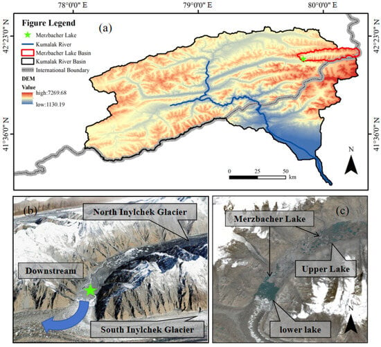
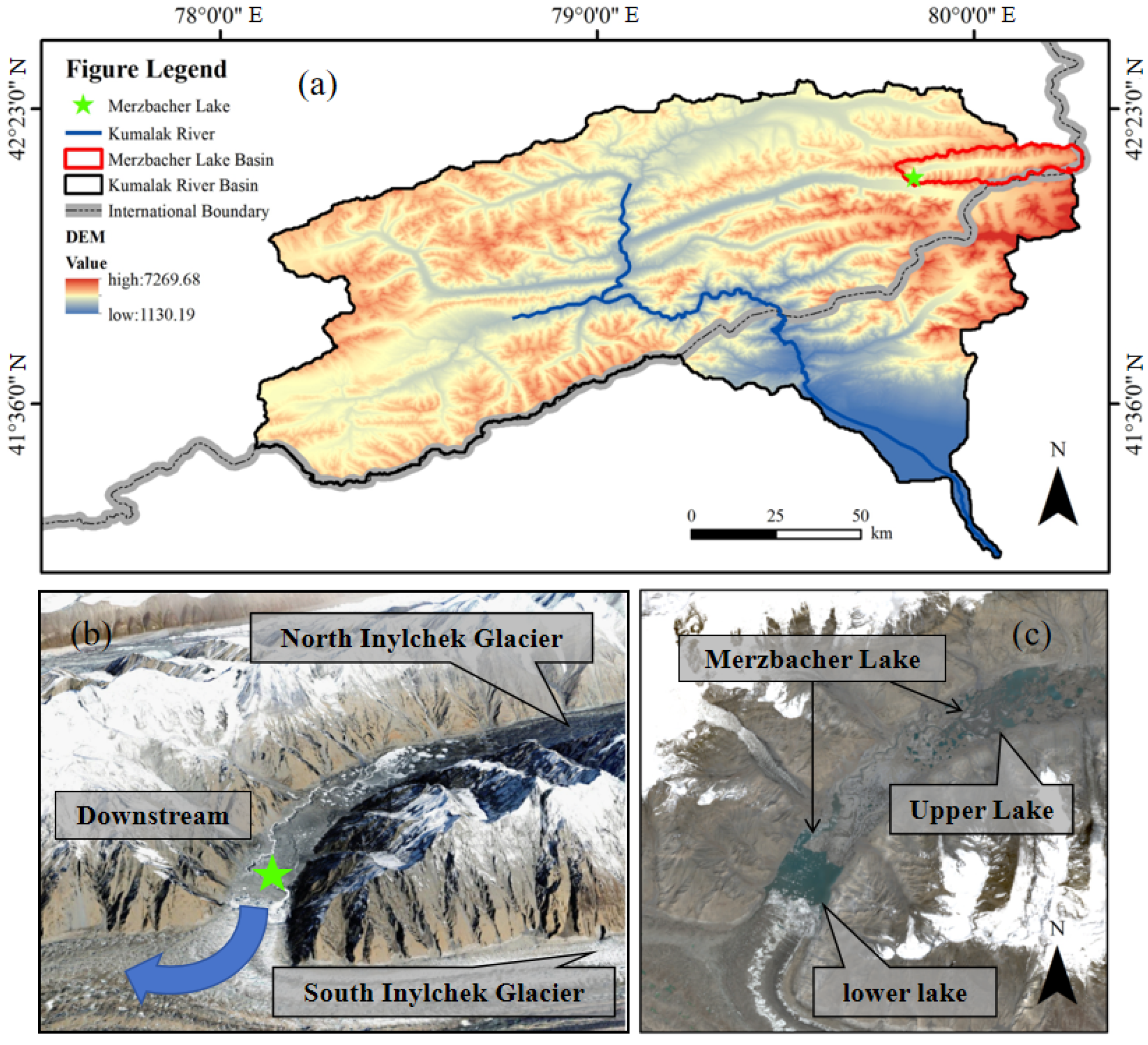
The Kumaraka River basin, located in the remote and topographically complex Tien Shan mountains of Central Asia, is a typical area prone to frequent glacial lake outburst floods [25,26], as shown in Figure 1a. Lake Merzbacher is situated on the border between Kyrgyzstan and the Xinjiang Uygur Autonomous Region of China, at approximately 42°12′02″N, 79°50′32″E. Its basin, the Kumaraka River basin, is a major tributary of the Aksu River. The drainage system of the basin exhibits a fan-shaped pattern, and the river channels are characterized by short courses and steep longitudinal gradients.
Figure 1.
Overview of the study area. (a) The Kumaraka River basin. (b) A 3D visualization of the lake and surrounding glaciers. (c) The Merzbacher Lake.
The 3D visualization in Figure 1b clearly illustrates the unique geomorphological setting that facilitates the lake’s formation: the advancing South Inylchek Glacier acts as a massive natural dam blocking the valley, while the retreat of the North Inylchek Glacier has created a large depression, providing the necessary accommodation space for meltwater accumulation [27]. Consequently, any outburst flood resulting from the lake’s instability would be characterized by high velocity, large volume, and significant destructive power, posing a severe threat to downstream areas. Figure 1c details the morphological characteristics of the lake itself, which appears as a dual-lake system composed of Upper Lake Merzbacher and Lower Lake Merzbacher, connected by a narrow channel. Lake Merzbacher exhibits a distinct cyclical outburst pattern: typically in late spring and early summer, as temperatures rise and snow and ice melt intensifies, the lake begins to fill. By around mid-July, the lake reaches its annual maximum area and volume, exerting peak pressure on the ice dam. Subsequently, within a period of a few days to a week, the lake water drains suddenly through subglacial channels or other mechanisms, generating an outburst flood.
To clearly define the scope of this study, any subsequent mention of Lake Merzbacher in this paper refers specifically to its lower basin (Lower Lake Merzbacher). The Lower Lake serves as the primary water storage body. During peak storage periods, it typically reaches a maximum surface area of approximately 2.5 km2, with a length of about 2.0 km and a width of roughly 1.0 km. All targeted remote sensing monitoring and risk assessment activities are focused exclusively on this one.
2.2. Data
2.2.1. GF-7 DLC
GF-7 is a sub-meter high-resolution optical stereo mapping satellite. The stereo imagery products acquired by its onboard Dual-Line Camera (DLC) serve as the foundation for the autonomous generation of the Digital Elevation Model (DEM) in this study. These products provide the high-quality, high-resolution stereo pairs essential for photogrammetric analysis, serving as the fundamental prerequisite and critical data foundation for generating a high-precision, high-timeliness 5 m resolution DEM of the lake basin.
2.2.2. Landsat
The Landsat series of satellites is an Earth observation program jointly managed by NASA (National Aeronautics and Space Administration) and the USGS (United States Geological Survey). Since 1972, it has continuously provided moderate-resolution imagery of the Earth’s surface, making it the longest-running and most widely used data source for global change research. For the time frame of this study, from 2018 to 2025, two satellites were primarily in operation: Landsat 8 and Landsat 9, both of which are equipped with the Operational Land Imager (OLI) and the Thermal Infrared Sensor (TIRS) [28]. This study utilizes the Level-2 Surface Reflectance products (Collection 2, Tier 1) acquired by these two satellites. These data provide multispectral bands at a 30 m spatial resolution, and the configuration of their key bands (e.g., green, near-infrared, shortwave infrared) enables the effective calculation of indices such as the NDWI and NDSI, which are fundamental for constructing the IWCI.
2.2.3. Sentinel-2
Sentinel-2 is a key representative of the high-resolution multispectral imaging mission under the European Space Agency’s (ESA) Copernicus Programme, comprising a constellation of two satellites (Sentinel-2A and Sentinel-2B). The mission is characterized by its high spatial resolution (up to 10 m), a high revisit frequency (approximately 2–3 days at the equator with the combined constellation), and a free and open data access policy. This study utilizes its Level-2A surface reflectance products.
2.2.4. Model Driving Data
This study selected four core physical variables: land surface temperature, snow cover, surface albedo, and precipitation. The data sources are detailed in Table 1.
Table 1.
Core Physical Variables and Sources.
- (1)
- LST (Land Surface Temperature)
This study uses the MODIS/Terra Daily Land Surface Temperature product (MOD11A1) as the foundational data for the thermal driving factors. This dataset provides daily daytime land surface temperatures with global coverage. LST directly reflects the temperature conditions of the ice and snow surface and is the most direct thermodynamic parameter driving its ablation, making it suitable for calculating key indicators such as Positive Accumulated Temperature (PAT). However, its validity is limited by cloud cover. Therefore, this study utilizes the product’s built-in Quality Assessment (QA) band for pixel-level quality control of the daily imagery, retaining only pixels flagged as ‘high quality’ or ‘clear sky’ for subsequent calculations.
- (2)
- SCA (Snow Cover Area)
This study employs the MODIS Daily Snow Cover product Version 6.1 (MOD10A1.061). The NDSI_Snow_Cover band is primarily used to retrieve the daily Snow Cover Area (SCA) and its rate of change over time within the upstream catchment of Lake Merzbacher. To ensure data reliability, an effective pixel mask was created using the QA information built into this band to exclude pixels contaminated by clouds, water bodies, sensor saturation, and other factors. Ultimately, only the total area of pixels clearly identified as ‘snow’ was calculated, thereby quantitatively assessing the intensity and dynamics of the snowmelt process.
- (3)
- Surface Albedo
This study utilizes the MODIS Daily Albedo product Version 6.1 (MCD43A3.061). The BRDF_Albedo_Band_Mandatory_Quality band is primarily used for quality control, and the White Sky Albedo (WSA) represented by the Albedo_WSA_shortwave band is extracted for analysis. By monitoring the decrease in the average catchment albedo, it is possible to determine whether the snowmelt process has entered an accelerated phase due to snow aging, metamorphosis, or dust contamination [29]. Similarly to the LST product, this study uses the product’s built-in QA information to perform pixel-level screening on the daily imagery, retaining only high-quality, cloud-free observations for subsequent statistical analysis, thereby providing the model with a reliable indicator of energy absorption efficiency.
- (4)
- Precipitation
To overcome the limitations of direct satellite precipitation observation due to cloud cover and to obtain spatiotemporally continuous precipitation information, this study uses NASA’s Global Land Data Assimilation System (GLDAS) as the precipitation data source. Specifically, the GLDAS Version 2.1 product driven by the Noah land surface model is selected. Through data assimilation techniques, this system integrates a variety of satellite and in situ observational data to generate a spatiotemporally seamless daily gridded precipitation dataset at a spatial resolution of 0.25 degrees [30]. This study extracts its total daily precipitation variable to accurately quantify the precipitation process, which acts as a direct input to the catchment’s water balance and a potential trigger for outbursts.
3. Methods
3.1. IWCI Construction and Glacial Lake Area Extraction
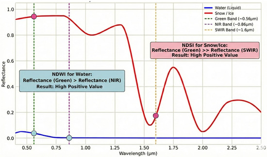
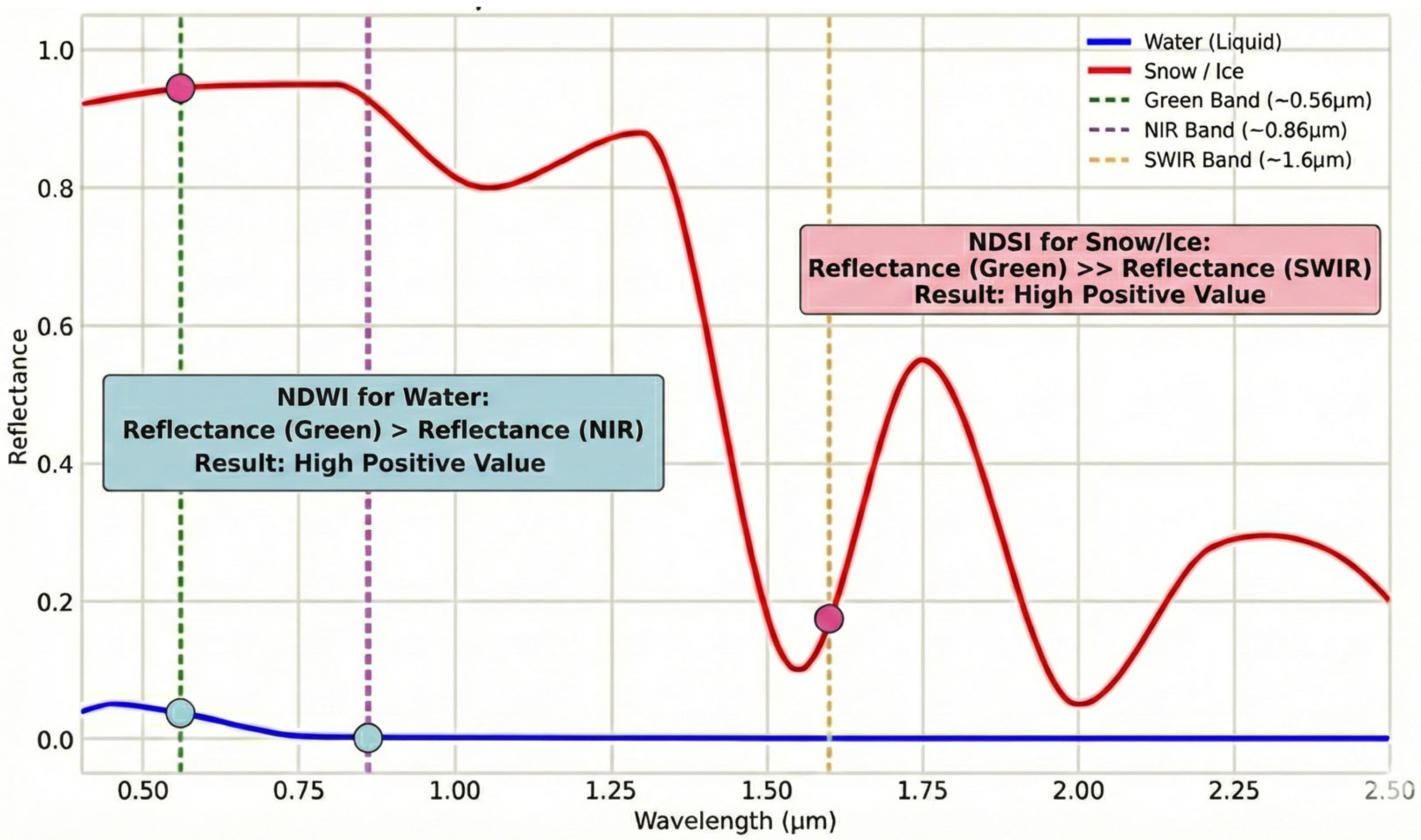
The differential spectral response of water and ice/snow across various bands provides the physical basis for constructing the remote sensing index. The spectral reflectance curves for water and ice/snow, along with the mechanism of the index, are illustrated in Figure 2, which was plotted using data from the United States Geological Survey (USGS) spectral library [31].
Figure 2.
Spectral reflectance curves of typical water and ice/snow. The blue and red curves represent water and ice, respectively, illustrating the construction logic of NDWI and NDSI.
The Normalized Difference Water Index (NDWI), as shown in Equation (1) (Green represents the surface reflectance in the Green band, and NIR represents the surface reflectance in the Near-Infrared band) [32], identifies water bodies by leveraging the strong absorption of liquid water in the Near-Infrared (NIR) band and its relatively high reflectance in the Green band. The Normalized Difference Snow Index (NDSI), as shown in Equation (2) (Green represents the surface reflectance in the Green band, and SWIR represents the surface reflectance in the Shortwave Infrared band.) [33], identifies ice and snow based on their strong absorption in the Shortwave Infrared (SWIR) band and high reflectance in the Green band.
During its cyclical filling process, the surface of Lake Merzbacher often exhibits a ‘mixed ice-water’ state, characterized by the coexistence of open water and disintegrated floating ice. This poses a significant limitation to methods that directly apply the NDWI for water body area extraction. When confronted with large areas of floating ice, the NDWI misclassifies them as non-water, resulting in a severe underestimation of the extracted water area. To address this challenge, this study innovatively develops the Ice-Water Composite Index (IWCI), as shown in Equation (3).
The IWCI, through a ratiometric operation, is designed to enhance the water signal using the NDWI while being normalized by the NDSI signal. This approach aims to generate a consistently high response over both ice and water pixels, thereby enabling the precise extraction of the total area of mixed-type glacial lakes.
Following the removal of negative values and normalization to a 0–1 range, the Otsu method [34] is applied to the IWCI result for threshold segmentation. This yields a global threshold T that optimally separates the glacial lake pixels (including both ice and water) from the non-lake background pixels. Once the overall lake extent is extracted, a DEM-based dynamic thresholding approach is employed for the fine-scale classification of ice and water. First, the DEM data are resampled to match the IWCI grid using cubic interpolation. Subsequently, within the lake mask, elevation values are stratified using the Jenks Natural Breaks algorithm [35]. For each elevation stratum, the corresponding IWCI values are grouped into two clusters (ice and water) using K-means clustering [36], which determines a locally optimal ice-water classification threshold.
Based on these discrete elevation-threshold pairs, a Support Vector Regression (SVR) model [37] is trained to construct a mapping function that accurately captures the complex non-linear relationship between elevation (h) and the classification threshold (T). Finally, a pixel-by-pixel classification is performed within the lake extent: for each pixel, its elevation is extracted and input into the mapping function to derive a unique dynamic threshold. This threshold is then compared with the pixel’s own IWCI value to classify it as either ice surface or water surface.
3.2. Glacial Lake Volume Curve Construction
An accurate digital model of the lake basin’s topography is a prerequisite for precisely estimating the effective water volume of Lake Merzbacher. Approaches for autonomously generating high-resolution DEMs primarily include Unmanned Aerial Vehicle (UAV) photogrammetry [38], Deep Learning (DL)-based stereo matching [39], and satellite stereo photogrammetry using the Semi-Global Matching (SGM) algorithm [40]. However, given that the Merzbacher basin is located in a complex, inaccessible alpine border zone lacking ground truth samples, UAV operations are logistically impossible and DL methods face high uncertainty. Consequently, this study adopts satellite stereo photogrammetry using GF-7 DLC imagery processed via the SGM algorithm. This method features the specific advantage of robust dense matching in low-contrast regions, which effectively overcomes texture homogeneity on ice and snow surfaces, thereby satisfying the rigorous requirement for reconstructing high-fidelity lakebed micro-topography in the absence of in situ data.
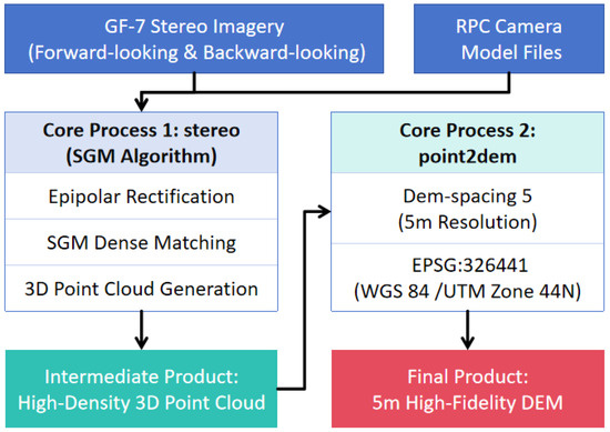
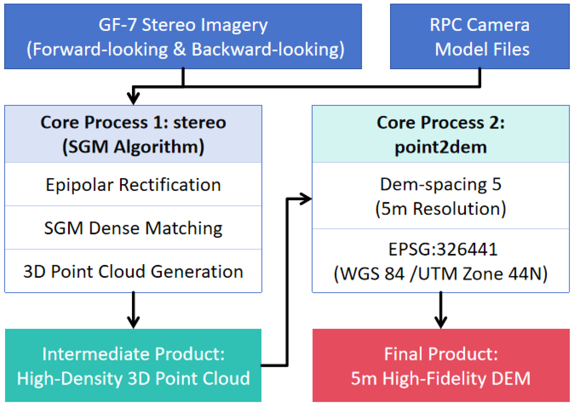
This study selected a GF-7 DLC stereo pair acquired on 23 November 2023, as the data source. This timing corresponds to Lake Merzbacher’s typical post-outburst empty phase, ensuring that the sensor could directly capture the exposed lakebed topography, providing an ideal data foundation for generating a high-fidelity bathymetric model. The DEM generation follows a standard satellite photogrammetry workflow: first, the initial imaging geometry model of the sensor is constructed using the RPC files provided with the imagery; second, the stereo pair is epipolar-rectified to facilitate stereo matching; third, the SGM algorithm is applied for high-density stereo matching [41] to generate a high-precision disparity map; fourth, a dense 3D point cloud is derived through space intersection, which is then interpolated to produce a regular-gridded 5 m resolution DEM. The aforementioned operations were all executed using the open-source toolkit ASP (Ames Stereo Pipeline) developed by NASA [42], with the workflow illustrated in Figure 3.
Figure 3.
Workflow of DEM generation. The workflow integrates SGM and point cloud interpolation to generate a 5 m DEM.
Based on the generated 5 m DEM, a Hypsometric Analysis was further employed to establish the lake’s area-volume relationship curve. The core of this method involves starting from the lowest point of the DEM and incrementally raising a virtual water level (i.e., elevation). At each level, the total area of the inundated pixels is calculated, and the corresponding water volume (storage) is computed through integration, thereby establishing a precise functional relationship between elevation, area, and volume.
3.3. Remote Sensing Time-Series Quantification of Driving Factors for Glacial Lake Outbursts
The cyclical outburst behavior of Lake Merzbacher is inherently linked to the hydro-thermal dynamics of its upstream catchment. Therefore, it is essential to extract key hydro-thermal driving factors from appropriate remote sensing data. The primary methods employed are detailed below.
3.3.1. Zonal Statistics and Raw Time-Series Generation
Following pixel-level quality control and masking of the daily raw remote sensing imagery, the two-dimensional raster data are converted into a numerical time series. This is achieved in a GIS environment by applying zonal statistics within the catchment boundary, which serves as the analysis mask. Different statistical operators are used according to the characteristics of the physical variables: for LST and Albedo, their spatial mean is calculated to reflect the overall thermodynamic and energy balance conditions of the catchment; for SCA and precipitation, their spatial sum is calculated to quantify the total material input to the basin.
3.3.2. Time-Series Smoothing and Reconstruction
To address the issues of “gaps” and “jitter” in the raw time series caused by factors such as cloud contamination, this study employs specific filtering and smoothing methods to interpolate and reconstruct the time series, generating complete, continuous curves that better represent the underlying physical processes. For LST and Albedo, the Savitzky–Golay (S-G) filtering method [43] is used for denoising and smooth reconstruction. For SCA, a combined approach of time-series smoothing and logical constraints is applied. After an initial smoothing with an S-G filter, the following logical constraint is imposed: during the primary melt season, if the snow cover area on a given day is greater than that of the previous day, it is forcibly corrected to be equal to the previous day’s value. This process generates a snow ablation curve that is both smooth and conforms to the monotonically decreasing physical process of snowmelt. For the precipitation time series, a 5-day moving average is applied to filter out single-day random noise and better reflect the actual cumulative contribution of a precipitation event to the catchment’s water budget.
3.3.3. Model Feature Engineering
To transform instantaneous daily scale observations into comprehensive physical indicators that reflect cumulative effects and time-lag dependencies, further feature extraction was performed on the daily data. These features can be categorized into three main types, representing heat accumulation that drives the melt process, indicating material supply and surface state changes, and identifying potential external event triggers. The final nine features are detailed in Table 2.
Table 2.
Model Driving Data Description.
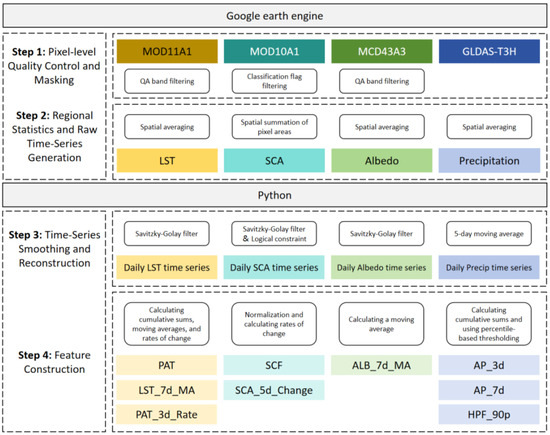
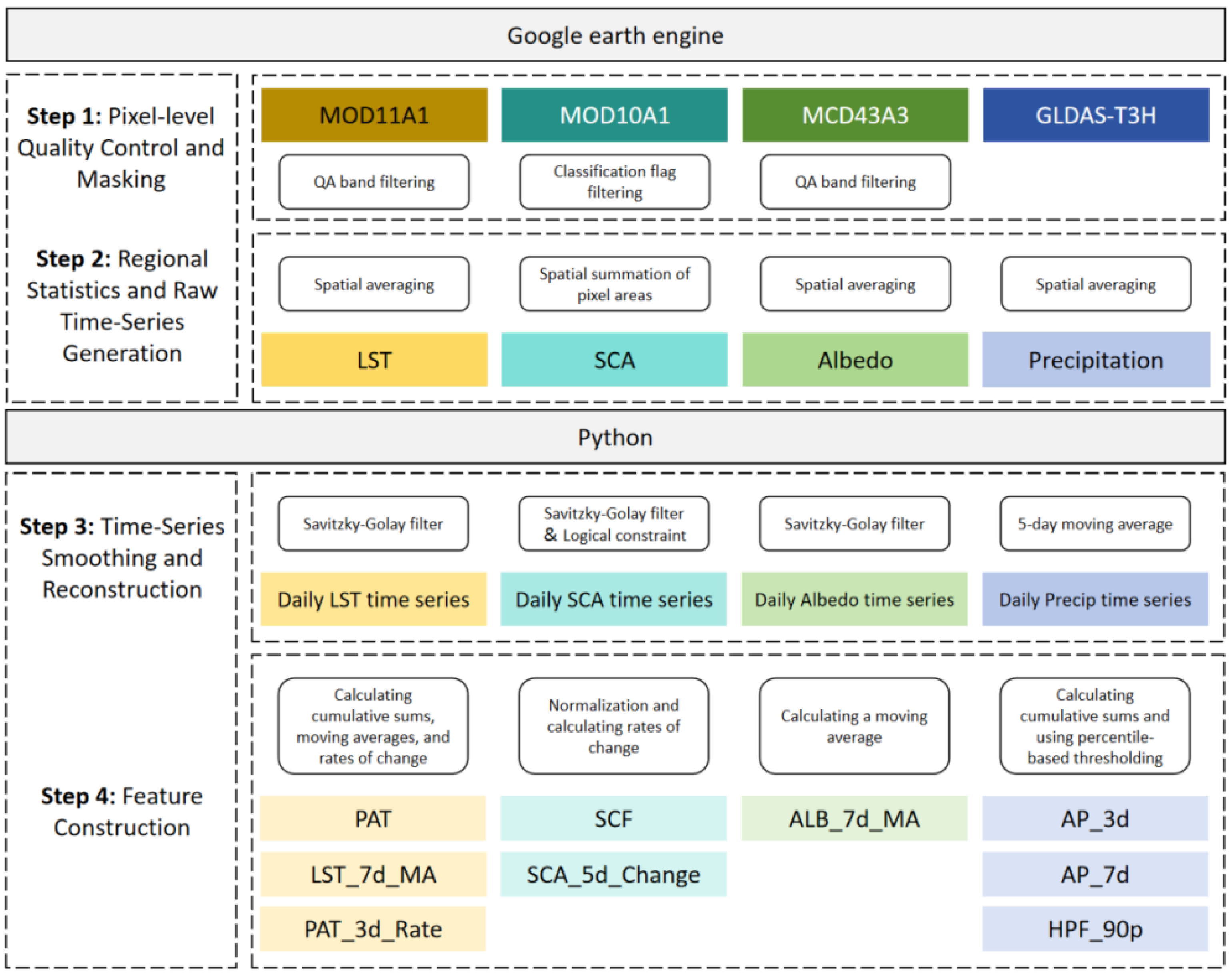
Google Earth Engine (GEE) is a geospatial analysis cloud platform that integrates a massive archive of multi-source remote sensing data with planetary-scale parallel computing capabilities, greatly simplifying the processing of large-scale, long-term time-series data. This study utilized GEE for processing the model driving data, with further optimization performed using Python3.9, as detailed in Figure 4.
Figure 4.
Model driving data preparation workflow. The process includes quality control, time-series reconstruction, and the calculation of nine hydro-thermal features.
3.4. Construction of the Dynamic Risk Assessment Model
This study develops and constructs a “remote sensing-driven empirical analysis framework.” The four pre-defined risk levels are shown in Table 3.
Table 3.
Risk Level Definitions.
Random Forest (RF) is an ensemble learning method particularly well-suited for this task. It can effectively handle the diverse, noisy, and highly non-linear remote sensing driver data involved in this study [44]. Furthermore, RF automatically captures complex interactions between factors. Crucially, while providing high prediction accuracy, its unique “feature importance” ranking function offers a means to objectively interpret the key physical mechanisms of glacial lake outbursts from a data-driven perspective. This study constructs the final modeling dataset by matching the nine features prepared in Section 3.3 (as independent variables) with the calculated water volumes from Section 3.2 (as the dependent variable) on a daily basis. To ensure the model focuses specifically on the lake-filling process under stable ice-dam conditions, the outburst day was defined as the date when water volume peaked and subsequently began a sharp decline. All data following this date until October 1st were excluded. This cut-off date was empirically determined based on historical records, indicating that the rapid drainage process typically concludes by this time as the lake transitions into the initial accumulation phase of the subsequent cycle. This data exclusion is critical because the accumulation phase is driven by hydro-thermal factors that increase volume, whereas the drainage phase is governed by the structural instability of the ice dam that causes rapid volume loss. Including data from the drainage phase would introduce conflicting training signals where high temperatures coincide with volume loss rather than gain, thereby preventing the algorithm from establishing a robust mapping for the risk incubation period. To objectively assess the model’s generalization ability, a time-series cross-validation method based on year splits is employed: data from 2018–2022 are used as the training set, while the datasets from 2023–2024 serve as the test set. The training set (2018–2022) comprises a total of 75 valid observational samples derived from cloud-free satellite imagery, with an annual distribution of 13 to 18 samples. To prevent model overfitting and optimize its performance, the Grid Search with K-Fold Cross-Validation method [45] is used to tune the model’s key hyperparameters. Referencing relevant research in hydrological and geological hazard prediction, this study focuses on systematically iterating through and optimizing four core hyperparameters, as detailed in Table 4.
Table 4.
Key Random Forest Hyperparameters.
The performance of different parameter combinations is evaluated through cross-validation, ultimately selecting the set of optimal hyperparameters that yields the strongest generalization capability for constructing the final predictive model. The final performance of the model is assessed by validation on the independent test set. The driver features from the test set are input into the optimally trained and tuned model to obtain daily predicted volume values. These predicted values are then compared against the actual lake volumes retrieved from remote sensing in the test set, and the accuracy is evaluated using three metrics: R2, RMSE, and MAE.
4. Results
4.1. Lake Merzbacher Area Extraction Results Based on the IWCI
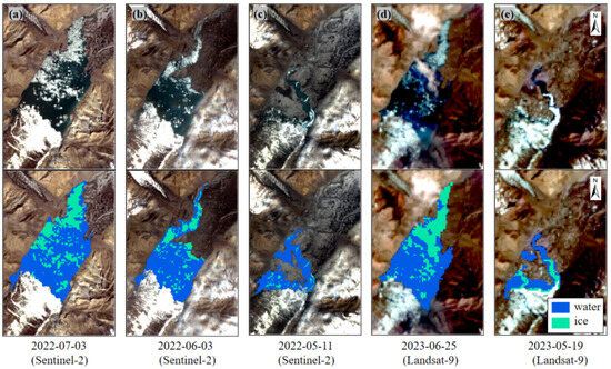
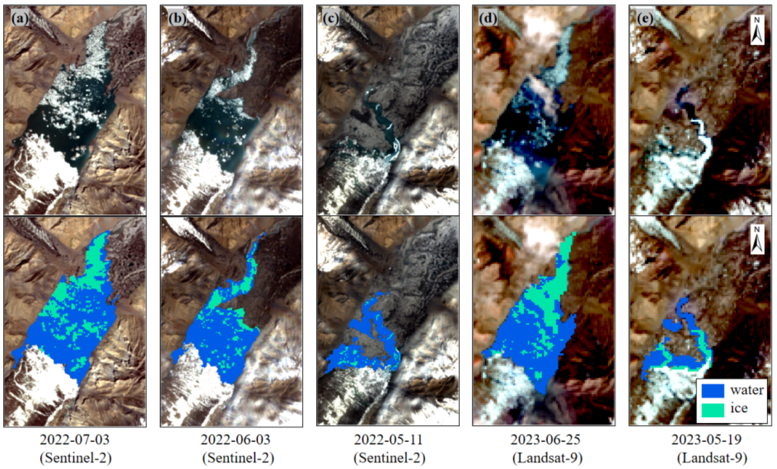
Five scenes of remote sensing imagery from different periods between 2022 and 2023 were selected. The IWCI was used to extract the glacial lake boundary and to classify ice and water. To quantitatively validate the extraction accuracy, we performed a random sampling of 25% of the classified pixels and cross-referenced them with the original RGB true-color imagery, where the distinction between ice, water, and land is visually evident. The validation yielded classification accuracies of 94.3% for water and 91.1% for ice, confirming the reliability of the proposed method.
Figure 5 illustrates the performance of the proposed IWCI ice-water extraction method across five different time phases. Subplots (a) through (e), respectively, show a comparison between the original remote sensing imagery (upper half) and the corresponding glacial lake extraction results (lower half) for different dates. From the perspective of multi-source data adaptability, the proposed IWCI method demonstrates consistent robustness when applied to different sensors (Sentinel-2 and Landsat 8/9). While Sentinel-2 imagery naturally offers finer boundary details due to its higher spatial resolution (10 m), the primary objective of integrating these diverse datasets is to construct a dense time-series. This synergy allows us to overcome the limitations of individual sensor revisit cycles and cloud cover, ensuring continuous monitoring of the rapid lake dynamics which is critical for dynamic risk assessment.
Figure 5.
Lake Merzbacher area extraction results based on the IWCI. (a–c) Extraction results from Sentinel-2. (d,e) Extraction results from Landsat-9. Blue and cyan represent water and ice, respectively.
Regarding the extraction performance at different filling stages, when the lake is near or at its full-storage period (as shown in Figure 5a,b,d), the boundary between the water body and the shoreline is distinct, and the distribution of ice and water within the lake is clear. In these cases, the method achieves high-precision boundary extraction and ice-water classification. However, during the initial filling stage (as shown in Figure 5c,e), the lower water level exposes extensive mudflats and bedrock, leading to more complex mixed-pixel phenomena along the water’s edge. Although the method can still effectively identify the main ice and water extents, its extraction accuracy is somewhat reduced compared to the full-storage period.
Notably, the South Inylchek Glacier, visible at the southern end of the lake, acts as a perennial ice dam. As its physical properties are stable and it is not the subject of this study, it was masked out in advance and excluded from the water body extraction calculations to ensure the accuracy of the analysis.
4.2. Storage Curve Development and Volume Calculation
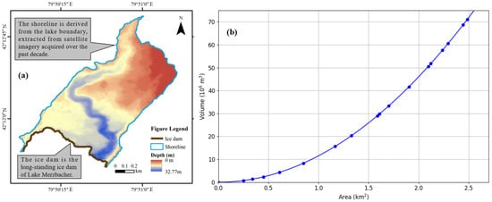
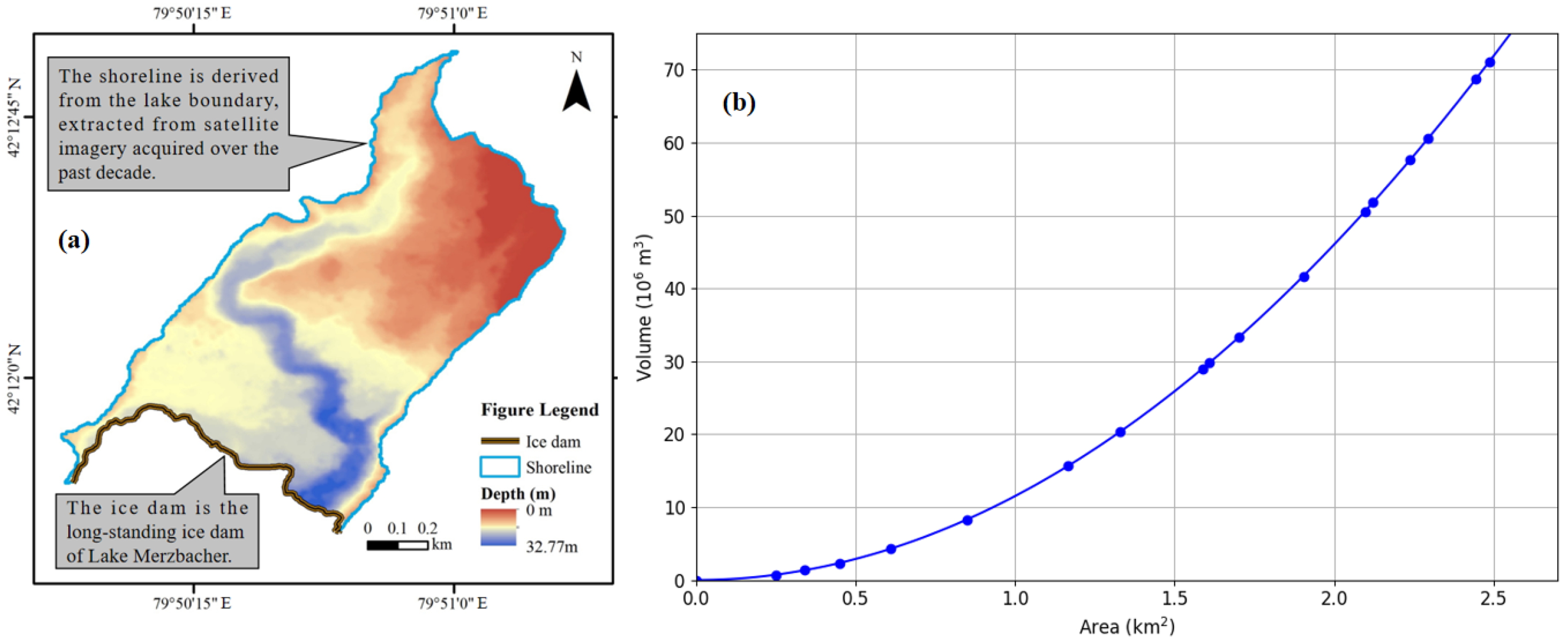
Utilizing a Gaofen-7 (GF-7) stereo pair acquired on 23 November 2023, this study successfully generated a 5 m resolution DEM of the Lake Merzbacher basin through ASP processing. This DEM was used to map the lake’s bathymetry, as shown in Figure 6a. Concurrently, the lake’s area-volume relationship curve was constructed using Hypsometric Analysis, as presented in Figure 6b.
Figure 6.
(a) Bathymetry of Lake Merzbacher. (b) The Area-Volume relationship curve.
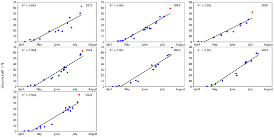
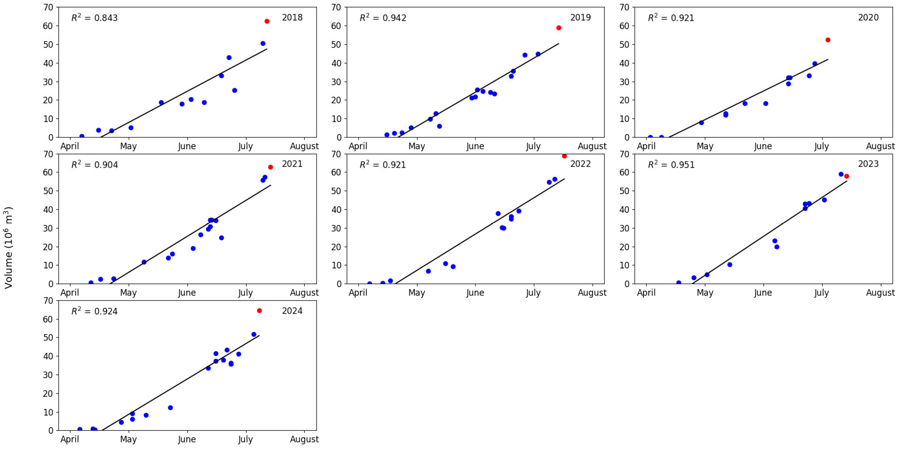
Analysis of the figure reveals that the morphology of the lower Lake Merzbacher basin is highly irregular, exhibiting a narrow, elongated shape oriented north–south, a form closely related to glacial erosion and damming processes. The lakebed is not flat but features multiple depressions and subglacial terraces of varying depths. The deepest region is located in the south-central part of the basin, near the front of the South Inylchek Glacier which acts as the ice dam; the legend indicates that the maximum water depth in this area can exceed 30 m. From this deepest point, the lakebed elevation gradually rises towards the north, east, and west, with complex slope variations. This “south-deep, north-shallow, centrally-depressed” topographic profile dictates that during the initial filling stage, water first accumulates in the southern trough before gradually inundating the shallower areas to the north as the water level rises. The extent of this DEM is defined by a perimeter shoreline that represents the lake’s maximum extent near full storage, determined from a multi-temporal analysis of satellite imagery over the past decade. Its southern boundary is sealed by a robust moraine dam, a perennial feature that not only provides the natural barrier for water accumulation but is also the critical section subject to localized instability and erosion during outburst events. By combining the derived storage curve with the area extraction results, a time series of the lake’s water storage for select dates between 2018 and 2024 was calculated (Figure 7). This dataset serves as the foundational ground truth for the subsequent development and validation of the predictive model.
Figure 7.
Scatter Plot of Simulated Water Storage Results (2018–2024). (Blue dots: observed volumes; Red dots: maximum observable water storage).
4.3. Quantitative Results of Remote Sensing Datasets
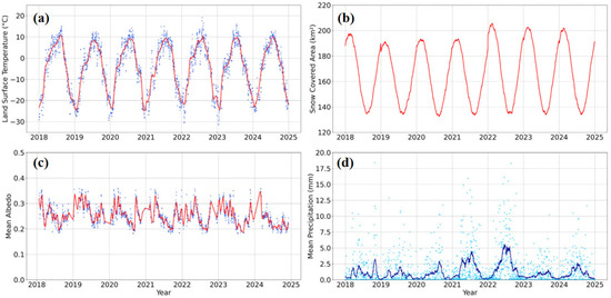
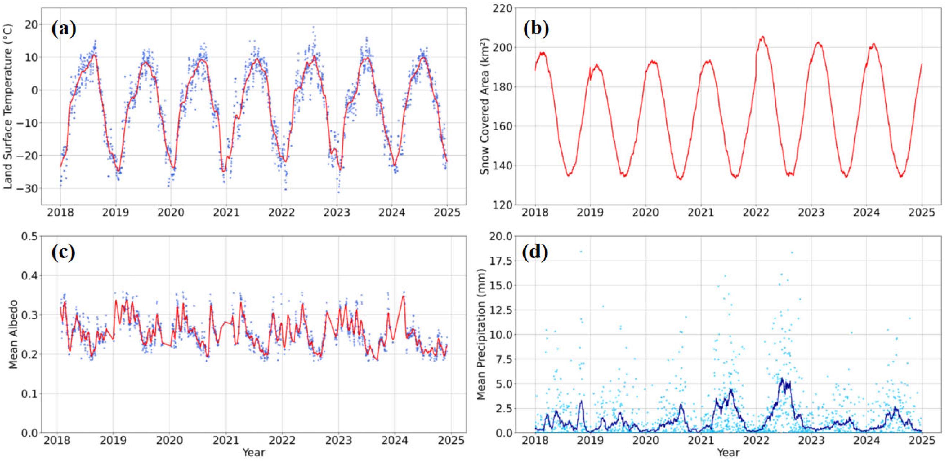
The time-series analysis of the four key physical variables—Land Surface Temperature (LST), Snow Cover Area (SCA), Surface Albedo, and precipitation—systematically demonstrates the feasibility of reconstructing the chain of core drivers for the Lake Merzbacher outburst cycle using publicly available remote sensing products, as illustrated in Figure 8.
Figure 8.
Time series plots of quantified remote sensing datasets. (a) Land Surface Temperature. (b) Snow Cover Area. (c) Mean Albedo. (d) Precipitation. (Blue dots: raw observations; Solid lines: reconstructed series).
The seasonal warming cycle of LST and the U-shaped ablation curve of SCA exhibit a distinctly coupled relationship, quantitatively revealing that heat accumulation is the fundamental force driving the filling of the glacial lake. More critically, the inverted U-shaped annual cycle of surface albedo, which is synchronized with the reduction in snow cover, intuitively demonstrates the positive feedback mechanism inherent in the glacial melt process: namely, that snow aging and bare ice exposure lead to a decrease in albedo, which enhances the surface’s absorption of solar radiation and thus accelerates meltwater runoff. Concurrently, the processed precipitation sequence successfully identifies the annual periods of concentrated rainfall, which can serve as potential external triggers.
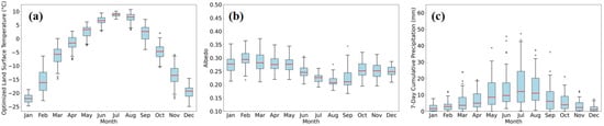
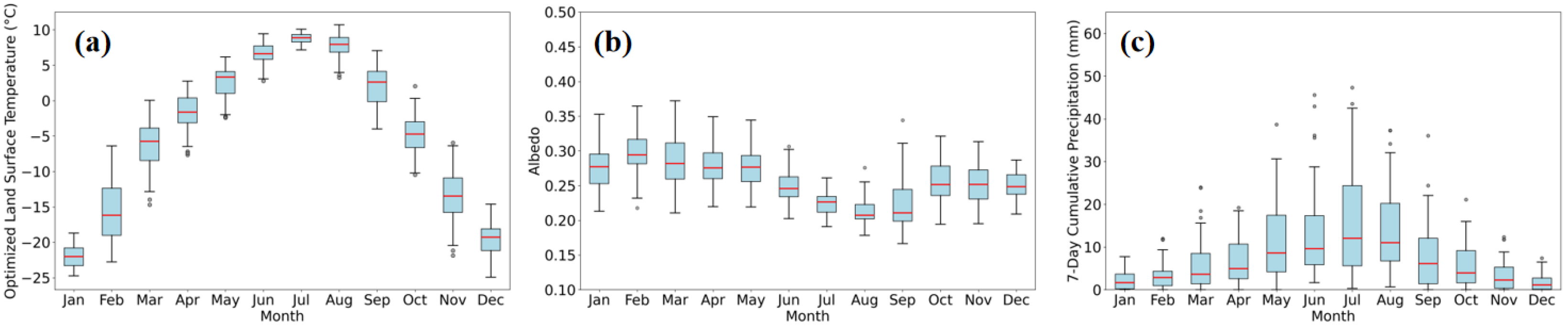
An analysis of the monthly statistical distributions for LST, Albedo, and 7-day cumulative precipitation further confirms the stability and viability of these remote sensing-derived datasets as inputs for the model. The box plot results presented in Figure 9 distill multi-year daily observations into monthly distribution characteristics with clear statistical significance. By representing the central tendency through multi-year medians and capturing variability via the interquartile range, this statistical aggregation effectively filters out inter-annual random fluctuations. This process minimizes the impact of anomalies from specific years such as extreme weather events, thereby highlighting the stable and long-term seasonal climatology that is essential for robust model training. Each key driving factor exhibits a prominent and stable seasonal cycle: the monthly distribution of LST clearly delineates the transition from the low-temperature frozen period to the high-temperature ablation period; the variation in the monthly medians and interquartile ranges of Albedo quantifies the seasonal shift in the surface energy balance state; and the statistical distribution of 7-day cumulative precipitation reveals a trend of increased heavy rainfall events later in the melt season. These stable and distinguishable monthly statistical features demonstrate the potential of the extracted remote sensing factors as predictive variables, capable of providing effective discriminatory information for the machine learning model to differentiate between the various risk stages of the glacial lake. Therefore, this analysis goes beyond merely demonstrating the efficacy of the data processing methods; it provides critical statistical validation of feature suitability for machine learning. The box plots reveal two key characteristics: first, the high inter-annual stability confirms that the driver sequences are not dominated by random noise or artifacts; second, the distinct seasonal separability indicates that the features possess strong discriminative power regarding the lake’s hydro-thermal status. These statistical properties are essential for the model to effectively learn the underlying physical patterns. Consequently, we conclude that these driver sequences, derived from public remote sensing products, are sufficiently robust and informative for building a reliable, data-driven dynamic risk assessment model for glacial lake outbursts.
Figure 9.
Box plots of key driving factors. (a) Land Surface Temperature. (b) Mean Albedo. (c) 7-day Cumulative Precipitation. (Red lines: medians; Boxes: interquartile ranges; Dots: outliers).
4.4. Model Results
To construct a model with optimal predictive performance and robust generalization capability, this study first employed a K-fold cross-validation with a grid search to systematically optimize the four key hyperparameters of the Random Forest model. These parameters (NE, MD, MSP, and MSL) collectively govern the model’s complexity, learning behavior, and resilience to overfitting. The optimization process determined that the model achieved its best-performing and most stable configuration when NE was 200, MD was 15, MSP was 5, and MSL was 2.
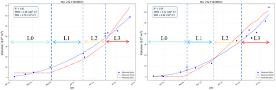
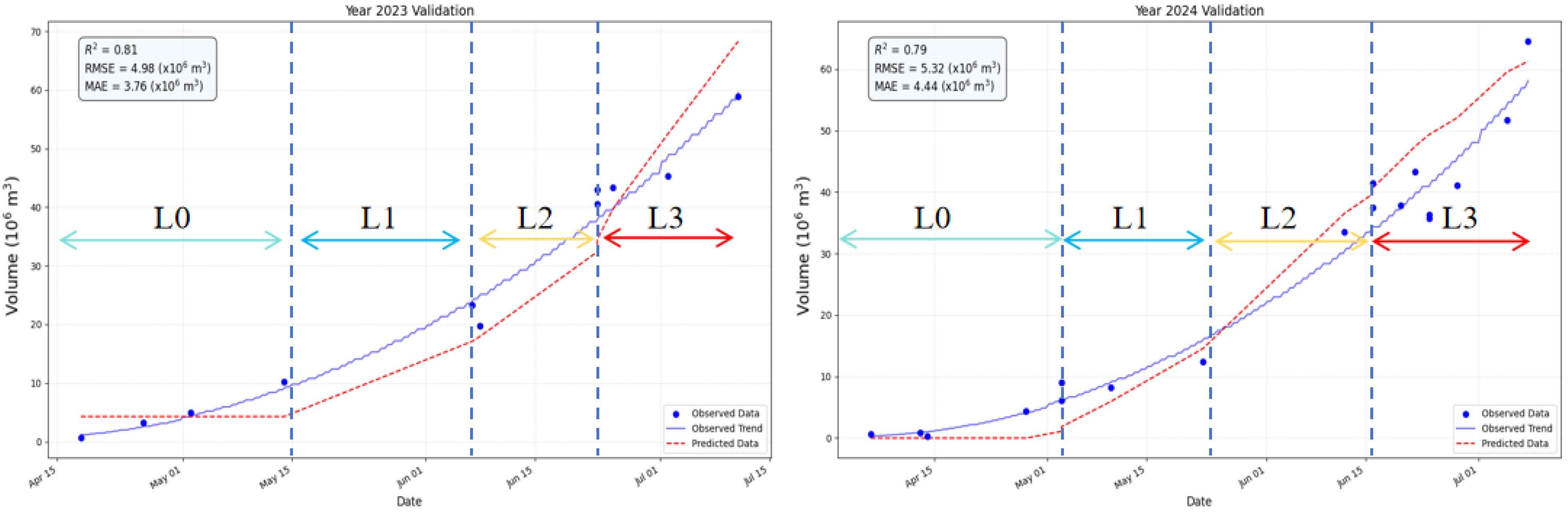
The final model was subsequently constructed using these optimal parameters, trained on data from 2018–2022, and validated against independent datasets from 2023 and 2024. The validation results and corresponding predicted storage curves are presented in Figure 10.
Figure 10.
Model validation results for 2023 and 2024. (Blue dots: observed data; Red dashed lines: model predictions; L0–L3: risk levels representing Routine Monitoring, Risk Incubation, High-Risk Alert, and Impending-Failure).
Considering the lake’s maximum volume of approximately 60 × 106 m3, this level of error provides a reliable quantitative foundation for the subsequent dynamic risk level classification. The model’s core value extends beyond these aggregate statistics, demonstrating a strong capability for dynamically simulating the water-filling process for specific years and enabling automated risk level classification.
Both 2023 and 2024 demonstrated consistent risk level progressions. From April to early May, the model’s predicted volume accurately corresponds to the “Normal Monitoring Period” (L0), when the lake basin is essentially empty. From mid-May onward, the predicted volume exhibits a continuous upward trend, closely tracking the energy-driven “Risk Incubation Period” (L1). More critically, the model demonstrates significant application value by automatically identifying the transition into the “High-Risk Warning Period” (L2) when the predicted volume surpasses the predefined danger threshold in early July. This capability provides crucial warning information for downstream disaster prevention and mitigation. The model’s accurate prediction of the peak volume and its timing also provides a key decision-making benchmark for identifying the “Impending Outburst State” (L3).
To gain deeper insight into the model’s internal decision-making mechanisms and its correlation with physical processes, this study further evaluated the model’s driving factors (Table 5). The importance of each input feature varies significantly, allowing them to be clearly stratified into three echelons.
Table 5.
Driving Factor Importance Scores.
The first echelon, acting as the core drivers, consists of PAT, SCA_5d_Change, and LST_7d_MA. PAT, as the most important factor, confirms from a data-driven perspective that the total heat accumulation over the entire melt season is the fundamental and controlling factor determining the annual meltwater total and the final lake volume. Meanwhile, SCA_5d_Change and LST_7d_MA represent the recent melt intensity and thermal conditions, respectively, which determine the daily “increment” of the lake volume. The model’s ability to capture this combined pattern of “long-period control” dominated by PAT and “short-term response” determined by immediate factors is key to its precise simulation of daily scale volume changes.
The second echelon, comprising state regulators, includes SCF, ALB_7d_MA, and PAT_3d_Rate. These factors do not directly generate meltwater themselves; rather, they describe the physical state of the catchment, thereby regulating the efficiency and potential of meltwater production. For example, SCF represents the available “material storage” for melting, while ALB_7d_MA reflects the surface’s efficiency in absorbing solar radiation, which aligns with the snowmelt positive feedback mechanism revealed in Section 4.3.
The third echelon consists of the three precipitation-related factors (AP_7d, AP_3d, HPF_90p), all of which have importance scores between 0.04 and 0.05. This result indicates that during the filling process of Lake Merzbacher, the contribution of direct liquid precipitation to the total lake volume is limited. The analysis suggests that the role of precipitation events is likely not as a major contributor to the lake’s volume. Instead, it is more plausible that they act as an external trigger when the lake is already at a high water level, inducing instability by altering the internal physical state of the ice dam.
5. Discussion
The core contribution of this study is the development of a GLOF prediction framework, driven entirely by multi-source remote sensing data and capable of dynamic risk assessment. The framework’s innovation is threefold: first, it resolves the challenge of lake area extraction under mixed ice-water conditions through the novel Ice-Water Composite Index (IWCI). Second, it overcomes the dependency on generic DEMs (which often lack timeliness and precision) by autonomously generating a high-fidelity lake basin DEM from GF-7 DLC data. Finally, it establishes an end-to-end non-linear response model using machine learning, linking remotely sensed daily lake volumes to quantified upstream hydro-thermal drivers. Importantly, the quantitative analysis results indicate that, despite the typically data-scarce alpine setting of Lake Merzbacher, the results obtained from zonal statistics based on remote sensing products within the upstream catchment are relatively reliable. These results represent key parameters that have a strong correlation with GLOF physical processes, making it feasible to construct a machine learning-based disaster assessment model based on them. This finding not only validates the feasibility of our methodology but also lays a solid data foundation for the model, thereby providing a complete technical paradigm for dynamic early warning in un-gauged, data-scarce regions.
This study builds upon the extensive foundation of previous research on Lake Merzbacher, attempting to provide a complementary solution from a different perspective. Prior studies have offered several key perspectives for understanding this complex system. One line of research has focused on simplifying complex physical processes into macro-indicators correlated with the final disaster; for example, Xie et al. [46] developed a comprehensive ‘hazard index’ by monitoring lake area and floating ice cover, while Kingslake et al. [47] established quantitative relationships between meteorological factors and the annual outburst timing using statistical models. Another line of research has concentrated on the fine-scale monitoring of the lake system’s physical state. Yan et al. [48] analyzed the influence of glacier velocity on the lake, focusing on the ice dam itself. The work of Gu et al. [49] is particularly notable, as they utilized multi-source, high-resolution satellite data for highly detailed monitoring of lake area and ice crevasse evolution, providing an invaluable, high-precision observational baseline for subsequent research.
Although these studies achieved significant progress in their respective directions and commonly point to thermal conditions as a key control factor, they remain essentially descriptive, correlational, or based on single-indicator macro-prediction. They did not culminate in a comprehensive model framework capable of ex-ante dynamic prediction of the core risk indicator: lake volume. The framework of this study is positioned to be complementary to this body of work. In contrast to the approaches of Xie et al. [46] and Kingslake et al. [47], which focused on predicting an abstract index or a final outburst date, our study directly predicts the daily evolution of lake volume—the physical quantity at the core of the hazard’s potential energy—providing a more direct and quantitative basis for risk assessment. In contrast to the approaches of Yan et al. [48] and Gu et al. [49], which centered on fine-scale monitoring of the physical state, our study shifts the scientific question from descriptive to predictive. The aforementioned studies provide a crucial, high-fidelity characterization of the lake system’s status quo, with a scientific focus on diagnostic analysis; our study, conversely, aims to establish a prognostic capability to simulate the future evolution of this state under specific hydro-thermal drivers. In this light, our research attempts to utilize a machine learning model as a non-linear transfer function, linking detailed remote sensing ‘observations’ with an understanding of the intrinsic physical ‘mechanisms,’ thereby aiming to explore a systematic and operable data-driven pathway for dynamic early warning for this specific lake.
Although this framework has been demonstrated to be effective, as an empirical model driven purely by remote sensing, it possesses inherent limitations that also define clear directions for future research. The model’s current prediction accuracy is constrained by the spatial resolution of its input driving factors, and its extrapolation capability when encountering extreme climatic events beyond the historical record remains untested. Therefore, future research will be dedicated to deepening this work in three primary areas: First, the core objective is to integrate this predictive framework with Numerical Weather Prediction (NWP) models, facilitating a shift from the current ‘simulation’ to true ‘forecasting’ and thus greatly extending the effective early warning time window. Second, we will further explore multi-source data fusion and downscaling techniques to acquire driver fields at higher spatiotemporal resolutions, aiming to enhance model precision. Finally, future work will prioritize applying this framework to glacial lakes equipped with in situ hydrological stations. This will allow for rigorous cross-validation against ground truth data, thereby solidifying the model’s reliability and paving the way for a regional dynamic early warning network.
6. Conclusions
Addressing the significant risk posed by the cyclical outbursts of Lake Merzbacher in the Central Asian Tien Shan and the limitations of traditional in situ monitoring in this region, this study developed and validated a dynamic glacial lake risk assessment model framework driven entirely by multi-source remote sensing data. This framework aims to transform glacial lake risk assessment from static hazard cataloging into a fine-grained, dynamically updatable process of simulation and prediction.
The framework first overcomes the challenges of inaccurate area extraction in mixed ice-water regions and the lack of high-precision basin topography by utilizing an innovative Ice-Water Composite Index (IWCI) and stereo imagery from China’s Gaofen-7 (GF-7) satellite. This enables the precise retrieval of daily glacial lake volume. Subsequently, through systematic feature engineering, nine key hydro-thermal driving factors were quantified from multi-source remote sensing products. A non-linear response model between these drivers and the lake volume was then established using the Random Forest (RF) machine learning algorithm.
The model results demonstrate that the framework possesses good predictive performance and reliability. On an independent validation set, the model achieved an R2 of 0.8 for lake volume prediction, accurately capturing the complete dynamic process from the initial filling stage to the near-peak stage. More importantly, the model’s feature importance analysis reveals from a data-driven perspective that Positive Accumulated Temperature (PAT) is the dominant factor controlling the lake’s filling cycle, while the contribution of precipitation is minimal, providing key quantitative evidence for understanding the lake’s physical mechanisms.
In conclusion, this study not only proposes an effective set of technical methods but also constructs a complete application framework, from data acquisition to risk level determination. This framework directly links high-precision volume prediction capabilities with pre-defined risk levels, achieving dynamic risk assessment. It circumvents the reliance on in situ observations and has the advantages of being low-cost and highly transferable. It provides a reference case for shifting from ‘static assessment’ to ‘dynamic early warning’ for GLOF disaster management in other data-scarce, high-risk glacial lake regions globally.
Author Contributions
Conceptualization, T.F. and X.L.; Methodology, T.F. and K.X.; Software, T.F., K.X., S.L. and L.C.; Validation, S.L.; Investigation, K.X. and L.C.; Resources, H.L.; Data curation, T.F. and H.L.; Writing—original draft, T.F. and X.L.; Writing—review & editing, T.F., X.L. and K.X.; Supervision, W.S., X.L. and K.X.; Project administration, W.S., X.L. and Y.L.; Funding acquisition, W.S., X.L. and Y.L. All authors have read and agreed to the published version of the manuscript.
Funding
Supported by the Special Project on Basic Scientific Research Funds of China Institute of Water Resources and Hydropower Research (Open bidding for selecting the best candidates) (JZ110145B0062025).
Data Availability Statement
All satellite remote sensing and field measured data used in this study are openly and freely available.
Conflicts of Interest
The authors declare that they have no known competing financial interests or personal relationships that could have appeared to influence the work reported in this paper.
References
- Zemp, M.; Huss, M.; Thibert, E.; Eckert, N.; McNabb, R.; Huber, J.; Barandun, M.; Machguth, H.; Nussbaumer, S.U.; Gärtner-Roer, I.; et al. Global glacier mass changes and their contributions to sea-level rise from 1961 to 2016. Nature 2019, 568, 382–386. [Google Scholar] [CrossRef] [Scilit]
- Harrison, S.; Kargel, J.S.; Huggel, C.; Reynolds, J.M.; Shugar, D.H.; Betts, R.A.; Emmer, A.; Glasser, N.; Haritashya, U.K.; Klimeš, J.; et al. Climate change and the global pattern of moraine-dammed glacial lake outburst floods. Cryosphere 2018, 12, 1195–1209. [Google Scholar] [CrossRef] [Scilit]
- Carrivick, J.L.; Tweed, F.S. A global assessment of the societal impacts of glacier outburst floods. Glob. Planet. Change 2016, 144, 1–16. [Google Scholar] [CrossRef] [Scilit]
- Taylor, C.; Allen, S.; Carrivick, J.L.; Quincey, D.J.; Mergili, M.; Shugar, D.H.; Haritashya, U.K.; Kargel, J.S.; Vilímek, V.; Watson, C.S.; et al. Glacial lake outburst floods threaten millions globally. Nat. Commun. 2023, 14, 1985. [Google Scholar] [CrossRef] [Scilit] [PubMed]
- Xu, H. Modification of normalised difference water index (NDWI) to enhance open water features in remotely sensed imagery. Int. J. Remote Sens. 2006, 27, 3025–3033. [Google Scholar] [CrossRef] [Scilit]
- Dozier, J. Spectral signature of alpine snow cover from the Landsat Thematic Mapper. Remote Sens. Environ. 1989, 28, 9–22. [Google Scholar] [CrossRef] [Scilit]
- Huggel, C.; Kääb, A.; Haeberli, W.; Teysseire, P.; Paul, F. Remote sensing based assessment of hazards from glacier lake outbursts: A case study in the Swiss Alps. Can. Geotech. J. 2002, 39, 316–330. [Google Scholar] [CrossRef] [Scilit]
- Vancutsem, C.; Ceccato, P.; Dinku, T.; Connor, S.J. Evaluation of MODIS land surface temperature data to estimate air temperature in different ecosystems over Africa. Remote Sens. Environ. 2010, 114, 449–465. [Google Scholar] [CrossRef] [Scilit]
- Hall, D.K.; Riggs, G.A.; Salomonson, V.V.; DiGirolamo, N.E.; Bayr, K.J. MODIS snow-cover products. Remote Sens. Environ. 2002, 83, 181–194. [Google Scholar] [CrossRef] [Scilit]
- Pradhan, R.K.; Markonis, Y.; Vaca Godoy, M.R.; Villalba-Pradas, A.; Mastrotheodoros, T.; Posadas, A.N.; Papa, F.; Kumar, R.; Lakshmi, A.K.; Felsch, P.; et al. Review of GPM IMERG performance: A global perspective. Remote Sens. Environ. 2022, 268, 112754. [Google Scholar] [CrossRef] [Scilit]
- Wang, Z.; Zhong, R.; Lai, C.; Chen, J. Evaluation of the GPM IMERG satellite-based precipitation products and the hydrological utility. Atmos. Res. 2017, 196, 151–163. [Google Scholar]
- Vuichard, D.; Zimmermann, M. The 1985 catastrophic drainage of a moraine-dammed lake, Khumbu Himal, Nepal: Cause and consequences. Mt. Res. Dev. 1987, 7, 91–110. [Google Scholar] [CrossRef] [Scilit]
- Huggel, C.; Kääb, A.; Haeberli, W.; Teysseire, P.; Paul, F. Regional-scale GIS-models for assessment of hazards from glacier lake outbursts: Evaluation and application in the Swiss Alps. Nat. Hazards Earth Syst. Sci. 2003, 3, 647–662. [Google Scholar] [CrossRef] [Scilit]
- Emmer, A. GLOFs in the WOS: Bibliometrics, geographies and global trends of research on glacial lake outburst floods (Web of Science, 1979–2016). Nat. Hazards Earth Syst. Sci. 2018, 18, 813–827. [Google Scholar] [CrossRef] [Scilit]
- Abdul Hakeem, K.; Abirami, S.; Rao, V.V.; Diwakar, P.G.; Dadhwal, V.K. Updated inventory of Glacial Lakes in Teesta Basin using remote sensing data for use in GLOF risk assessment. J. Indian Soc. Remote Sens. 2018, 46, 463–470. [Google Scholar] [CrossRef] [Scilit]
- Liu, H.; Wang, Z.; Wen, H.; Wang, G.; Zhang, T.; Li, J. Predicting glacial lake outburst susceptibility on the southern Tibetan Plateau with historical events and machine learning methods. Nat. Hazards 2025, 121, 17677–17705. [Google Scholar] [CrossRef] [Scilit]
- Zhou, B.; Zou, Q.; Jiang, H.; Liu, W.; Hu, G.; Liu, J.; Wang, J.; Yao, T. A novel framework for predicting glacial lake outburst debris flows in the Himalayas amidst climate change. Sci. Total Environ. 2024, 946, 174435. [Google Scholar] [PubMed]
- Veh, G.; Korup, O.; Walz, A. Hazard from Himalayan glacier lake outburst floods. Proc. Natl. Acad. USA 2020, 117, 907–912. [Google Scholar] [CrossRef] [Scilit]
- Chen, F.; Zhang, M.; Guo, H.; Allen, S.; Kropáček, J.; Ran, Y.H. Annual 30-meter dataset for glacial lakes in high mountain Asia from 2008 to 2017. Earth Syst. Sci. Data 2021, 13, 741–766. [Google Scholar] [CrossRef] [Scilit]
- Dubey, S.; Goyal, M.K. Glacial lake outburst flood hazard, downstream impact, and risk over the Indian Himalayas. Water Resour. Res. 2020, 56, e2019WR026533. [Google Scholar] [CrossRef] [Scilit]
- Ahmed, R. Glacial lake outburst flood (GLOF) hazard and risk management strategies: A global overview. Water Resour. Manag. 2025, 39, 1–16. [Google Scholar]
- Ahmed, R.; Sam, L.; Bhardwaj, A. It is time to build GLOF-resilient communities globally before another GLOF disaster strikes. NPJ Nat. Hazards 2025, 2, 41. [Google Scholar] [CrossRef] [Scilit]
- Narama, C.; Duishonakunov, M.; Kääb, A.; Daiyrov, M.; Abdrakhmatov, K. The 24 July 2008 outburst flood at the western Zyndan glacier lake and recent regional changes in glacier lakes of the Teskey Ala-Too Range, Tien Shan, Kyrgyzstan. Nat. Hazards Earth Syst. Sci. 2010, 10, 647–659. [Google Scholar] [CrossRef] [Scilit]
- Liu, J.; Li, Z.; Liu, Y. Glacier dammed lake outburst flood in cold season in the Tien Shan, China and Kyrgyzstan. arXiv 2023. [Google Scholar] [CrossRef] [Scilit]
- Shrestha, F.; Steiner, J.F.; Shrestha, R.B.; Huggel, C.; Frey, H.; Azam, M.F.; Quincey, D.J.; Miles, E.S.; Jackson, M.; Racoviteanu, A.; et al. A comprehensive and version-controlled database of glacial lake outburst floods in High Mountain Asia. Earth Syst. Sci. Data 2023, 15, 3941–3961. [Google Scholar] [CrossRef] [Scilit]
- Ye, Q.; Wang, Y.; Liu, L.; Liu, S.; Li, S.; Che, T.; Yang, T.; Zhang, X. Remote sensing and modeling of the cryosphere in high mountain Asia: A multidisciplinary review. Remote Sens. 2024, 16, 1709. [Google Scholar]
- Li, J.; Li, Z.W.; Wang, C.C.; Zhu, J.J.; Ding, X. Using SAR offset-tracking approach to estimate surface motion of the South Inylchek Glacier in Tianshan. Acta Geophys. Sin. 2013, 56, 1226–1236. [Google Scholar]
- Choate, M.J.; Rengarajan, R.; Hasan, M.N.; Barsi, J.; Chander, G.; Morfitt, R.; Arvidson, T. Operational aspects of Landsat 8 and 9 geometry. Remote Sens. 2023, 16, 133. [Google Scholar]
- Schaaf, C.; Wang, Z. MODIS/Terra+ Aqua BRDF/Albedo Daily L3 Global-500m V061. NASA EOSDIS Land Processes Distributed Active Archive Center (DAAC) Data Set, 2021: MCD43A3. 061. Available online: https://www.earthdata.nasa.gov/data/catalog/lpcloud-mcd43a3-061 (accessed on 20 December 2025).
- Wu, Z.; Feng, H.; He, H.; Zhou, J.; Zhang, Y. Evaluation of soil moisture climatology and anomaly components derived from ERA5-land and GLDAS-2.1 in China. Water Resour. Manag. 2021, 35, 629–643. [Google Scholar] [CrossRef] [Scilit]
- Kokaly, R.F.; Clark, R.N.; Swayze, G.A.; Livo, K.E.; Hoefen, T.M.; Pearson, N.C.; Wise, R.A.; Benzel, W.; Lowers, H.A.; Driscoll, R.L.; et al. USGS Spectral Library; version 7; US Geological Survey: Reston, VA, USA, 2017.
- Gao, B.C. NDWI—A normalized difference water index for remote sensing of vegetation liquid water from space. Remote Sens. Environ. 1996, 58, 257–266. [Google Scholar]
- Salomonson, V.V.; Appel, I. Development of the Aqua MODIS NDSI fractional snow cover algorithm and validation results. IEEE Trans. Geosci. Remote Sens. 2006, 44, 1747–1756. [Google Scholar] [CrossRef] [Scilit]
- Liu, D.; Yu, J. Otsu method and K-means. In Proceedings of the 2009 Ninth International Conference on Hybrid Intelligent Systems, Shenyang, China, 12–14 August 2009; Volume 1, pp. 344–349. [Google Scholar]
- Chen, J.; Yang, S.T.; Li, H.W.; Zhang, B.; Lv, J.R. Research on geographical environment unit division based on the method of natural breaks (Jenks). Int. Arch. Photogramm. Remote Sens. Spat. Inf. Sci. 2013, 40, 47–50. [Google Scholar] [CrossRef] [Scilit]
- Kodinariya, T.M.; Makwana, P.R. Review on determining number of Cluster in K-Means Clustering. Int. J. 2013, 1, 90–95. [Google Scholar]
- Awad, M.; Khanna, R. Support vector regression. In Efficient Learning Machines: Theories, Concepts, and Applications for Engineers and System Designers; Apress: Berkeley, CA, USA, 2015; pp. 67–80. [Google Scholar]
- Deliry, S.I.; Avdan, U. Accuracy of unmanned aerial systems photogrammetry and structure from motion in surveying and mapping: A review. J. Indian Soc. Remote Sens. 2021, 49, 1997–2017. [Google Scholar] [CrossRef] [Scilit]
- Yang, J.; Xu, J.; Lv, Y.; Zhou, C.; Zhu, Y.; Cheng, W. Deep learning-based automated terrain classification using high-resolution DEM data. Int. J. Appl. Earth Obs. Geoinf. 2023, 118, 103249. [Google Scholar] [CrossRef] [Scilit]
- Gehrke, S.; Morin, K.; Downey, M.; Newby, M.; Boehm, J. Semi-global matching: An alternative to LIDAR for DSM generation. In Proceedings of the 2010 Canadian Geomatics Conference and Symposium of Commission I, Calgary, AL, Canada, 15–18 June 2010; Volume 2. [Google Scholar]
- Tatar, N.; Arefi, H.; Hahn, M. High-resolution satellite stereo matching by object-based semiglobal matching and iterative guided edge-preserving filter. IEEE Geosci. Remote Sens. Lett. 2020, 18, 1841–1845. [Google Scholar] [CrossRef] [Scilit]
- Beyer, R.A.; Alexandrov, O.; McMichael, S. The Ames Stereo Pipeline: NASA’s open source software for deriving and processing terrain data. Earth Space Sci. 2018, 5, 537–548. [Google Scholar] [CrossRef] [Scilit]
- Schafer, R.W. What is a savitzky-golay filter? [lecture notes]. IEEE Signal Process. Mag. 2011, 28, 111–117. [Google Scholar] [CrossRef] [Scilit]
- Rigatti, S.J. Random forest. J. Insur. Med. 2017, 47, 31–39. [Google Scholar] [CrossRef] [Scilit]
- Yan, T.; Shen, S.L.; Zhou, A.N.; Chen, J.J.; Lyu, H.M.; Wu, H.N. Prediction of geological characteristics from shield operational parameters by integrating grid search and K-fold cross validation into stacking classification algorithm. J. Rock Mech. Geotech. Eng. 2022, 14, 1292–1303. [Google Scholar] [CrossRef] [Scilit]
- Xie, Z.; Shangguan, D.; Zhang, S.; Wu, P.; Zhang, X.; Li, H. Index for hazard of Glacier Lake Outburst flood of Lake Merzbacher by satellite-based monitoring of lake area and ice cover. Glob. Planet. Change 2013, 107, 229–237. [Google Scholar]
- Kingslake, J.; Ng, F. Quantifying the predictability of the timing of jökulhlaups from Merzbacher Lake, Kyrgyzstan. J. Glaciol. 2013, 59, 805–818. [Google Scholar] [CrossRef] [Scilit]
- Yan, S.; Li, Y.; Li, Z.; Liu, J.; Hu, X. An insight into the surface velocity of Inylchek Glacier and its effect on Lake Merzbacher during 2006–2016 with Landsat time-series imagery. Environ. Earth Sci. 2018, 77, 773. [Google Scholar] [CrossRef] [Scilit]
- Gu, C.; Li, S.; Liu, M.; Wang, Z.; Lei, X.; Zhou, J.; Liu, F.; Wang, D.; Du, G. Monitoring glacier lake outburst flood (GLOF) of lake Merzbacher using dense Chinese high-resolution satellite images. Remote Sens. 2023, 15, 1941. [Google Scholar]

Disclaimer/Publisher’s Note: The statements, opinions and data contained in all publications are solely those of the individual author(s) and contributor(s) and not of MDPI and/or the editor(s). MDPI and/or the editor(s) disclaim responsibility for any injury to people or property resulting from any ideas, methods, instructions or products referred to in the content. |
© 2025 by the authors. Licensee MDPI, Basel, Switzerland. This article is an open access article distributed under the terms and conditions of the Creative Commons Attribution (CC BY) license.