Article

Comparison of Classic Classifiers, Metaheuristic Algorithms and Convolutional Neural Networks in Hyperspectral Classification of Nitrogen Treatment in Tomato Leaves

by
Brahim Benmouna
1,
Raziyeh Pourdarbani
2,
Sajad Sabzi
3,
Ruben Fernandez-Beltran
1,
Ginés García-Mateos
1,* and
José Miguel Molina-Martínez
4
1
Computer Science and Systems Department, University of Murcia, 30100 Murcia, Spain
2
Department of Biosystems Engineering, College of Agriculture, University of Mohaghegh Ardabili, Ardabil 56199-11367, Iran
3
Computer Engineering Department, Sharif University of Technology, Tehran 11155-1639, Iran
4
Food Engineering and Agricultural Equipment Department, Technical University of Cartagena, 30203 Cartagena, Spain
*
Author to whom correspondence should be addressed.
Remote Sens. 2022, 14(24), 6366; https://doi.org/10.3390/rs14246366
Submission received: 27 October 2022 / Revised: 27 November 2022 / Accepted: 13 December 2022 / Published: 16 December 2022
(This article belongs to the Special Issue Computer Vision and Machine Learning Application on Earth Observation)

Abstract

:
Tomato is an agricultural product of great economic importance because it is one of the most consumed vegetables in the world. The most crucial chemical element for the growth and development of tomato is nitrogen (N). However, incorrect nitrogen usage can alter the quality of tomato fruit, rendering it undesirable to customers. Therefore, the goal of the current study is to investigate the early detection of excess nitrogen application in the leaves of the Royal tomato variety using a non-destructive hyperspectral imaging system. Hyperspectral information in the leaf images at different wavelengths of 400–1100 nm was studied; they were taken from different treatments with normal nitrogen application (A), and at the first (B), second (C) and third (D) day after the application of excess nitrogen. We investigated the performance of nine machine learning classifiers, including two classic supervised classifiers, i.e., linear discriminant analysis (LDA) and support vector machines (SVMs), three hybrid artificial neural network classifiers, namely, hybrid artificial neural networks and independent component analysis (ANN-ICA), harmony search (ANN-HS) and bees algorithm (ANN-BA) and four classifiers based on deep learning algorithms by convolutional neural networks (CNNs). The results showed that the best classifier was a CNN method, with a correct classification rate (CCR) of 91.6%, compared with an average of 85.5%, 68.5%, 90.8%, 88.8% and 89.2% for LDA, SVM, ANN-ICA, ANN-HS and ANN-BA, respectively. This shows that modern CNN methods should be preferred for spectral analysis over other classical techniques. These CNN architectures can be used in remote sensing for the precise detection of the excessive use of nitrogen fertilizers in large extensions.

1. Introduction

A proper balance of chemical fertilizers is necessary to increase crop yield, enhance fruit quality, and provide plant disease resistance, in general. This is especially true in horticultural production, such as the focus of this study, which deals with tomato (Solanum lycopersicum L. var Royal) fields. This can be achieved by increasing organic matter in the soil, thereby providing the plants with the necessary nutrients. The main nutrients consumed by tomatoes are potassium (K), nitrogen (N2) and calcium (Ca), among others [1]. A shortage in any one of these three macro-nutrients could weaken the plant and lower tomato fruit quality. Due to excessive nitrogen consumption, the tomato taste and soluble solid content may also decrease, and its acidity may rise [2]. Overall, a high amount of nitrogen decreases plant resistance to many diseases. High nitrogen levels, particularly those in the form of ammonium, will cause blossom end rot disease. An excessive amount of nitrogen can also result in leaf curling, excessive flowering with falling flowers, excessive vegetative growth, poor fruit production and, eventually, decreased yield [3].
In the area of crop monitoring, automatic physiological abnormality detection in products is a key topic. Additionally, as millions of kilograms of toxic solution are applied annually to treat diseases, efforts should be taken to limit the use of toxics that are harmful for both human health and the environment. For this purpose, the agricultural applications of remote sensing using satellites and drones can be a powerful tool, especially those based on hyperspectral remote imaging [4].
For several years, image processing has been used to diagnose crop diseases, including leaf diseases and others [5,6,7,8,9]. For example, Agarwal et al. [6] proposed a shortened CNN system including eight hidden layers. The authors concluded that the model outperformed previously pre-trained models. A precision of 98.4% was achieved. Additionally, they developed an approach based on convolutional neural networks to identify cucumber disease. Their suggested algorithm achieved an accuracy of 93.75% after being trained using different sets of hyperparameters [7]. In the majority of cases, early detection could not be achieved. The development of spectroscopy made it possible to extract a product’s internal features. In essence, spectroscopic methods use the physical characteristics of electromagnetic field and wave interactions with materials, such as absorption, transmission, reflection, phosphorescence, radioactive decay and fluorescence, to offer fingerprint details of the biological sample [8,9].
Healthy and diseased plants can also be distinguished by near infrared (NIR) spectroscopy [10,11,12]. Even if spectroscopy alone offers good spectral resolution in the Vis-NIR range of wavelengths, it does not contain spatial information. On the other hand, hyperspectral images give both spatial and spectral information of imaging objects. In effect, hyperspectral images can be viewed as a combination of spectroscopy and computer vision techniques [13,14]. These techniques that combine artificial intelligence and hyperspectral images have had many applications in agriculture, some of which are summarized next. Hyperspectral imaging was applied by Pan et al. [14] to study the early identification of pear fruit blight due to Alternaria alternata fungus. Spectral mapping was conducted to segment the infected region and to analyze the pathogenicity of the disease. The ability to diagnose disease using support vector machine (SVM), k-nearest neighbor (KNN) and partial least squares regression (PLSR) models has been developed and tested. The accuracy of the SVM model was 97.5% according to the results. Yu et al. [15] examined the use of hyperspectral imaging and machine learning techniques to detect mercury stress in tobacco. Features regarding the texture and appearance of the tobacco plant were analyzed. The status of mercury-stressed plants was estimated using partial least squares discriminant analysis (PLS-DA) and support vector machines (SVMs). Confusion matrices and receiving operating curve (ROC) were used to assess the performance of the models. The results demonstrated a great success in the detection of stressed tobacco plants by heavy mercury when hyperspectral imaging and machine learning techniques were combined.
Xia et al. [16] used hyperspectral images to detect the waterlogging stress in rapeseed. The result demonstrated that the deep learning neural network classification was more precise than the RGB image. They suggested creating a spectroscopic monitoring process with a high-performance efficient spectrum sensor. Although most of the recent deep learning classifiers on hyperspectral images are commonly based on patch-wise classification, they can be inefficient because of the redundant computations between adjacent patches. For this purpose, Xu et al. [17] proposed a spectral–spatial fully convolutional network, which is able to process a hyperspectral image at pixel level. This architecture avoids the extraction of patches, but it can obtain similar results to other patch-wise methods.
Jun et al. [13] examined cadmium deposits in the leaves of tomato based on Vis-NIR spectral images. The authors came to the conclusion that Vis-NIR hyperspectral imaging had great potential for identifying the content of heavy elements in tomato leaves under various levels of cadmium stress. Qing et al. [18] discovered tomato spotted wilt virus (TSWV) also applying hyperspectral images and artificial intelligence algorithms. Three techniques—boosted regression tree (BRT), genetic algorithm (GA) and support vector machine (SVM)—were examined in the range from 400 to 1000 nm with 128 bands of infected and healthy plants. According to the obtained results, the models created using the BRT algorithm achieved the best accuracy, reaching 85.2%. Anthracnose was identified in tea plants by [19]. The detection rate for the disease-sensitive bands at 754, 686 and 542 nm was 98%. A challenge that research on hyperspectral images must address is the availability of large databases of labeled images. The process of the pixel-level labelling of images is costly and time-consuming, so some approaches have been proposed to use semi-supervised methods in deep learning applications. For example, Xu et al. [20] developed a robust self-ensembling network (RSEN), which consists in two deep subnetworks working together with both labeled and unlabeled hyperspectral images, achieving state-of-the-art results in remote sensing datasets.
As mentioned above, the control of abnormalities and diseases of agricultural goods is made possible through the early detection of nutritional disorders. The present work aims to study the early detection of nitrogen excess using a non-destructive hyperspectral imaging approach. The main difference between the present study and other similar ones is the use of pixel-by-pixel information of hyperspectral images. For this purpose, a set of varied classifiers is applied, ranging from classic supervised methods (linear discriminant analysis (LDA) and support vector machines (SVMs)), hybrid approaches that combine artificial neural networks (ANNs) and metaheuristic algorithms (independent component analysis (ICA), harmony search (HS) and the bees algorithm (BA)) and four different structures of convolutional neural networks (CNNs), always using images at different wavelengths from 400 to 1100 nm. Since the proposed method works at pixel-level, it can be applied to remote sensing hyperspectral imaging.

2. Materials and Methods

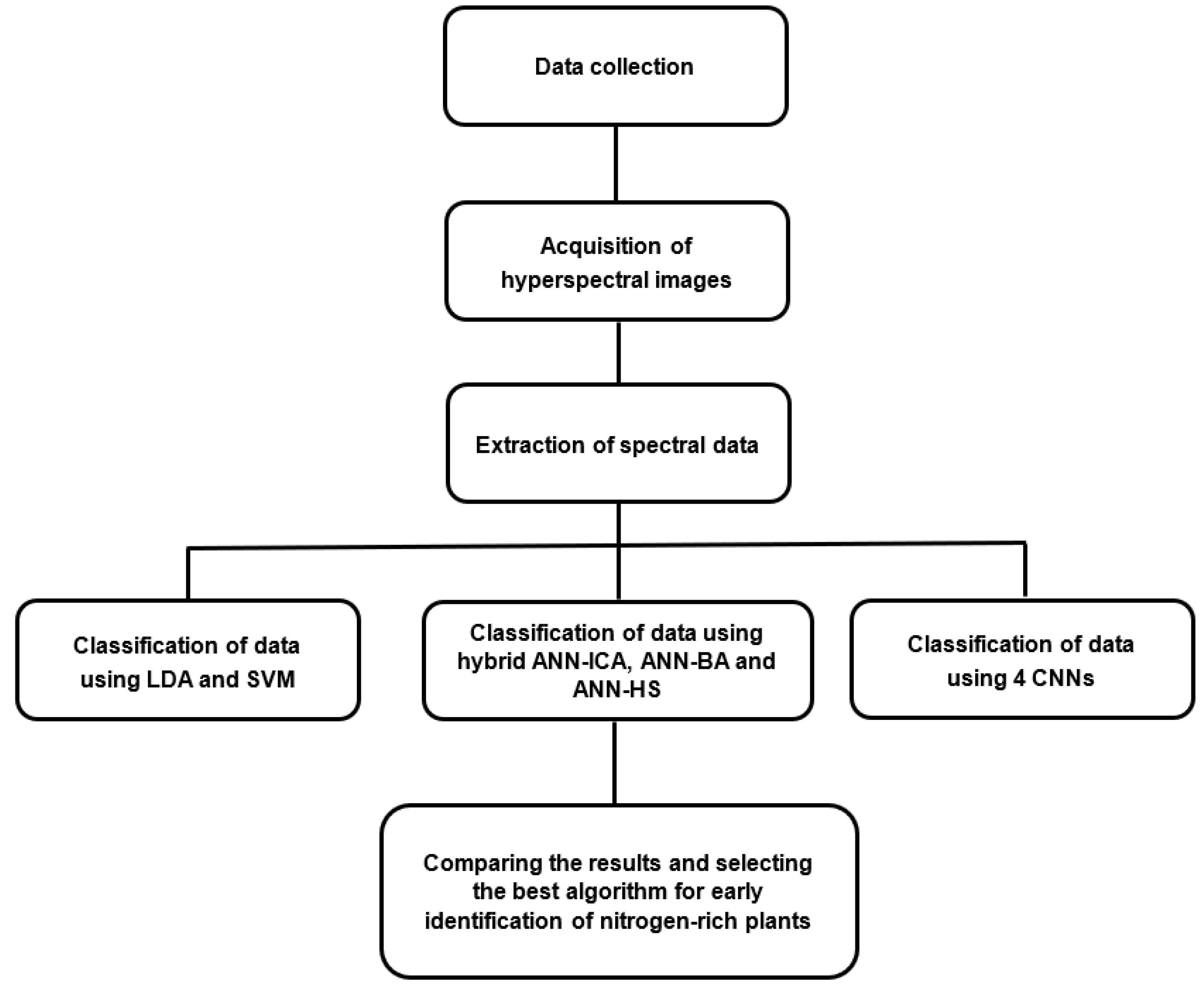
Figure 1 depicts the flowchart of the different stages of the research methodology applied in the present work for the detection of excess nitrogen in tomato plants. These stages are described in detail in the following subsections.

2.1. Data Collection by Planting Tomato in Pots

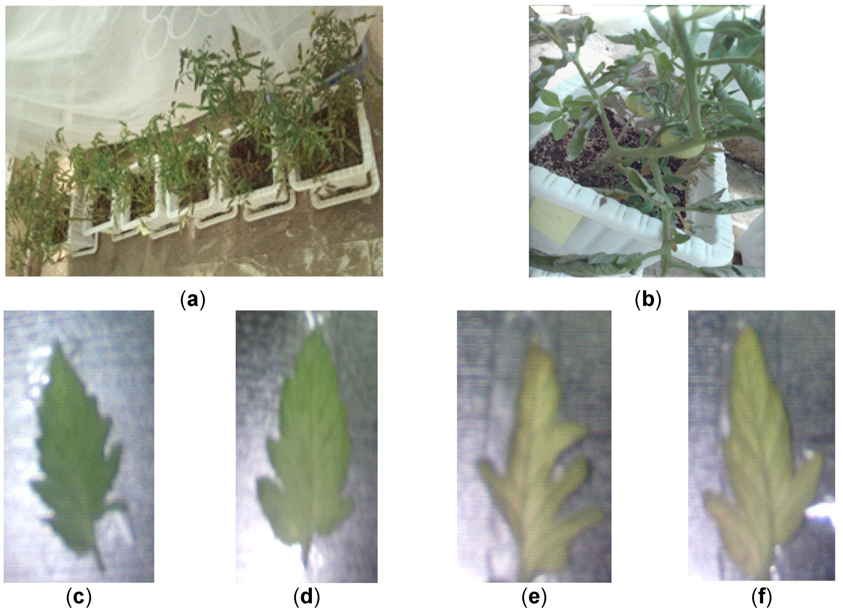
Tomato seeds of Royal variety were initially placed in each of the 20 prepared pots (Figure 2). All the pots received the same amounts of water and fertilizers until the leaves of the plant grew (after about three months of planting). After that, an overdose of nitrogen by 30% (2.6 g per pot, in the form of ammonium nitrate dissolved in irrigation water) was applied to half of the pots; the other half were the control pots. Then, a hyperspectral camera VIRA1000 (described in the following subsection) in the range of visible and near-infrared spectrum was used to capture images of 10 randomly selected leaves from each pot each day. This sampling process continued until there were visible signs of nitrogen-excess on the leaves. Due to the fact that the leaves were pale and twisted after 3 days (72 h), sampling was conducted over the course of 3 days.
This process resulted in 4 classes, with the names of A for the control pots (normal nitrogen fertilizer), and B, C and D for the treatment pots after 1, 2 and 3 days of nitrogen over-dose, respectively. To identify which day the algorithm would be able to detect more precisely the nitrogen-rich leaves, the classification algorithm was categorized by these sampling days. In total, we obtained hyperspectral images of 100 leaves for each class.
It can be seen in the samples of Figure 2 that the effect of nitrogen excess was not visually evident after only 1 day of treatment (Figure 2d), while the decoloring of the leaves was clear after 3 days (Figure 2f). The symptoms could be observed in some leaves after 2 days (Figure 2e) but not in all the cases. Since the objective was to detect fertilizer over-application as early as possible, spectral information could be used for this purpose. There are two more reasons to use hyperspectral information instead of RGB data. First, the effect of decoloring in RGB images would not be able to distinguish between different types of pathologies in the plants, while spectral data could be used to obtain a spectral signature to detect nitrogen in the leaves. Second, since the ultimate objective was to apply these techniques with remote sensing data, this spectral signature can be used even if the leaves are not seen in detail in the images, which would not be possible for RGB images.

2.2. Hyperspectral Imaging and Extraction of Spectral Information

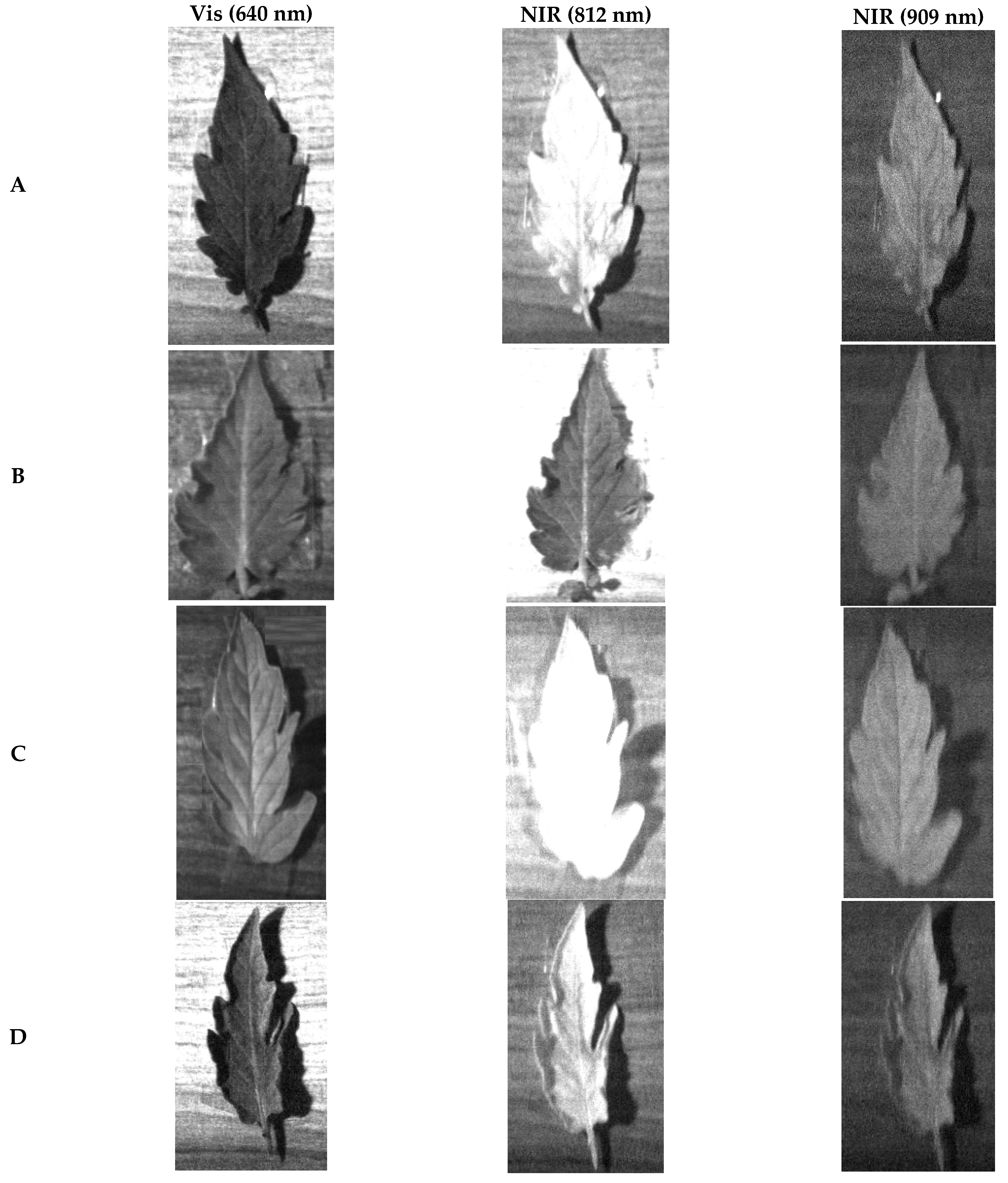
The hyperspectral camera used to capture hyperspectral images from the leaves was a model VIRA1000 (Noor Imen Tajhiz Co., www.hyperspectralimaging.ir, last accessed on 26 October 2022, Iran), specifically designed for research purposes. This camera was an angular scan-type, with a spectral range from 400 to 1100 nm. The spectral resolution of the camera was 2.5 nm, and the spatial resolution for an object at a distance of 1 m was 250 microns. Overall, the configuration of the hardware system to produce the images consisted of (1) the hyperspectral camera; (2) a laptop with an Intel Core i5-330M processor operating at a frequency of 2.13 GHz, 4 GB of RAM, Microsoft Windows 10; (3) a pair of tungsten halogen lights, SLI-CAL model (StellarNet, Tampa, FL, USA); and (4) a lighting chamber to remove noise caused by ambient light. The background of the capture chamber was dark wood (it is not the background shown in Figure 2). Some samples of the hyperspectral images captured are shown in Figure 3. For each leaf, the system captured 327 spectral images evenly spaced in the range of wavelengths from 400 to 1100 nm, including visible (Vis) and near-infrared (NIR) spectrum.

2.3. Pre-Processing of the Spectral Data

The obtained raw digital values were normalized using two calibration patterns named black body (an object with maximum absorption) and white body (an object with maximum reflection). The spectra of these bodies were measured with the hyperspectral camera. Then, the spectra of the samples for each band were normalized with respect to these calibration bodies, using Equation (1):
N o r m a l i z e d   s a m p l e   r e f l e c t a n c e = R a w   s a m p l e   r e f l e c t a n c e R a w   b l a c k   b o d y   r e f l e c t a n c e   R a w   w h i t e   b o d y   r e f l e c t a n c e R a w   b l a c k   b o d y   r e f l e n c a n t e
This process was repeated for each of the 327 spectral bands captured by the camera.
After calibration, the obtained normalized spectral values needed a pre-processing step to reduce the effects of noise such as ambient light. Therefore, Equation (2) was used to transform reflection spectral data into absorption one:
A b s o r p t i o n   s p e c t r a = l o g ( 1 R e f l e c t a n c e   s p e c t r a )
Light scattering was corrected using a standard normal variate with a wavelet modification. Smoothing was improved with the Savitzki–Golay filter [19]. These processes were carried out by Parles software, a popular chemistry software used for multivariate modeling [21].

2.4. Data Augmentation and Dataset Generation

Data augmentation is a logical technique to increase the dataset size by adding modified copies of formerly existing train data or newly created data from existing data [22]. It is a way to decrease overfitting when training a classification model. In fact, data augmentation is a strategy that enables dealing with the problem of limited data since much information is required by CNN methods to work properly. However, it must be clarified that data augmentation should be applied to the training and verification sets, not to the test set.
For this purpose, first, from the 100 leaves of each class, 70 leaves were randomly selected for training and validation and the remaining 30 leaves for testing. From each leaf, different patches of pixels were manually selected (about 3 patches per image). Then, from each patch a tuple of 327 values (the spectral bands) was computed. More specifically, we obtained 1144 patches for training and 489 for the test dataset.
Data augmentation was applied only on the training set, thus, producing 4842 samples. From them, we randomly selected 80% for training (3871) and 20% for validation (971). The data augmentation technique consisted of computing the weighted averages of two random samples of the same class. That is, for each class, we randomly took 2 of the original 327-valued tuples and computed a weighted average of both tuples; the new resulting tuple was added to the training set. This process was repeated until generating a proportion of about 3 synthetic samples for 1 original sample. So, for all the classification algorithms described in the following sections, the same training (3871 samples), validation (971 samples) and test (489 samples) sets were used.

2.5. Algorithms for Early Detection of Nitrogen-Rich Plants

In our proposed methodology, the problem of detecting nitrogen over-application was considered as a classification problem. The input to the system was the spectral data of the leaves. More specifically, the input was a 327-tuple of spectral values from the hyperspectral images taken by image patches after the application of the pre-processing and data augmentation process described in the previous sections. The output of the classifier was the treatment class—A, B, C and D—representing the number of days after nitrogen overdose, from 0 to 3, respectively.
In order to have a wide variety of methods to compare, nine different classifiers were tested. These methods include two classic machine learning classifiers, three hybrid approaches of neural networks and metaheuristic algorithms and four structures of convolutional neural networks. These methods are described in detail in the following sections.

2.5.1. Support Vector Machines (SVMs) Classifier

Support vector machines are a common supervised learning technique in the field of classification and regression. In the last decades, they were very popular as an alternative to perceptron neural networks, being applied in many different domains, such as classification problems in remote sensing [23]. The basis of the SVM classifier is the linear classification of data, in which the optimal hyperplane equation for the training data is computed by quadratic programming methods [24].
SVM uses a technique called kernel trick to convert the data and then finds the optimal boundary between possible outputs. In other words, it performs very complex conversions and then specifies how to separate your data based on the tags or outputs you define. In the experiments, the best selection of parameters for the SVM was selected by a process of trial and error. The linear kernel function was selected for the kernel of the system, and the C parameter (also known as the penalty parameter) was set to 1.

2.5.2. Linear Discriminant Analysis (LDA) Classifier

Linear discriminant analysis is one of the most powerful algorithms for reducing the size of information. In many cases, the amount of information and features is so large that it challenges classifiers that even if classification is possible, high accuracy is not achieved. LDA is closely related to principal components analysis (PCA). The two techniques search for a linear combination of variables that are able to describe the data. Additionally, LDA attempts to model differences between different data classes. LDA is used when the observations are continuous values [25,26]. For this purpose, two matrices are defined. The first matrix is for the samples of each class so that the average of each class is calculated, and then, the distance of all the samples with the average of the class is calculated and placed in the matrix. Now, the eigenvalues and eigenvectors are calculated in such a way that there is a minimum distance between the samples of each class and a maximum distance between the classes. Finally, each new sample is transferred to the reduced dimension by multiplying the transfer matrix.

2.5.3. Hybrid Artificial Neural Networks–Harmony Search (ANN-HS)

Three hybrid classification methods were added to the experiments. These methods rely on an artificial neural network (ANN) classifier, which takes the 327-tuple as input and produces the output class. However, it is well known that the structure of the ANN can greatly affect the obtained results [27]. The purpose of hybrid approaches is to select the best structure of layers for the ANN. In general, these methods consider the structure of the network as a tuple of values containing the number of hidden layers, the number of neurons per layer, the activation function of the layers, the backpropagation and the training functions. The hybrid method consists of a metaheuristic algorithm that selects different tuples (i.e., network configurations) and performs a training/test process with each configuration. The configuration that obtains the least mean squared error is selected as the optimal ANN for the classification. The difference between the proposed methods resides in the metaheuristic algorithms, which are responsible for deciding the configurations that are tested, following distinct evolutionary strategies. Three methods have been considered: harmony search, the bees algorithm, and the imperialist competitive algorithm.
The harmony search (HS) algorithm is a method inspired by music with the aim of coordination and harmony to achieve the best answer. Trying to find the harmony in music is like finding the optimal conditions in the optimization process. In fact, the HS process is the finest strategy for qualitatively transforming examined processes into tangible and quantitative optimization processes. A process with some ideal rules that will result in the transformation of a beautiful gamut of music into a suitable solution for solving various optimization problems [5].
In the HS algorithm, each solution is called a harmony and it is represented as an n-dimensional vector. An original population is first randomly generated and algorithmized in harmony memory (HM). Then, a response is selected based on memory rule consideration, pitch adjustment and random selection. Then, the obtained answer vector is compared with the worst harmony in the HM vector; if it is better, it will be replaced with the worst answer vector and will be updated. This process continues until the stop condition is met.
After the application of the hybrid ANN-HS method to the spectral training data of the tomato leaves, the obtained ANN structure is the one presented in Table 1. In all the ANN-based methods, the number of epochs was 200 and the learning rate 0.001.

2.5.4. Hybrid Artificial Neural Networks–Bees Algorithm (ANN-BA)

The bees algorithm (BA) was developed by Pham et al. [28]. The BA method mimics the food search behavior of a group of bees. In this model, the algorithm performs a type of neighborhood search combined with random search, and it can be used for either hybrid optimization or functional optimization.
Insects, called real bees, are social insects that live in hives. In a beehive, a specialized organization is assigned to bees to perform certain tasks for them. This organization objective is to maximize the amount of nectar in the colony to obtain the maximum food sources. Three different kinds of bees are represented in the model of food seeking by intelligent bee groups in a colony, including worker bees, observer bees and scout bees.
Worker bees are in charge of exploiting the nectar sources that have already been discovered, as well as giving information to the waiting bees (observer bees) in the hive about the food quality. Supervising bees stay in the hive and choose a food source to be exploited based on the information given by workers. On the other hand, scouts search randomly in the environment to find a new food source based on their intrinsic motivation or external or random evidence. So, the key steps of the BA algorithm are the following:
  • Initialize the location of food resources.
  • Each worker bee produces a new food source in its food source position and extracts a better source.
  • Each observer bee selects a source depending on the quality of its solution and produces a new food source at the position of the selected food source and selects a better source.
  • Determine the source that should be abandoned and allocate its workers as observers in search of new sources of food.
  • Remember the best source of food found up to now.
  • Repeat the steps from 2 to 5 until the stop criterion is appropriate.
The optimal network structure obtained by the application of the hybrid ANN-BA method is shown in Table 2.

2.5.5. Hybrid Artificial Neural Networks–Imperialist Competitive Algorithm (ANN-ICA)

The imperialist competitive algorithm (ICA) is based on machine intelligence that simulates human communities and tracks the optimal point to have a response for an optimization problem [29]. The method creates a mathematical model to solve the problem with a number of random elements, which are called country. The best of these countries (called elites) are designated as colonizers. The colonizers attract other elements called colonies towards them. The supremacy of an empire depends on the status of colonies. If the empire does not succeed in the colonial competition, it will be removed from the competition. So, the empire has to attract the colonies of other competing empires to assure its survival.
Table 3 contains the parameters of the optimal ANN selected by this hybrid ANN-ICA algorithm for the detection of nitrogen excess in the leaves. In this case, unlike the previous ones, the selected ANN only has 2 hidden layers.

2.5.6. Convolutional Neural Network Classifiers

Convolutional neural networks (CNNs) are a special type of neural network that consist of 3 main types of layers: convolution layers, pooling layers and fully connected layers. CNNs use less pre-processing than other image classification approaches, which means the network adopts criteria that were learned manually in previous approaches. This independence of CNNs from human manipulation and prior knowledge is an essential benefit of this technique [30]. In the present paper, four different structures of CNN were compared. All of them had a typical funnel structure, where the input tuple was successively reduced to a smaller size but with a greater number of features. Then, the values were flattened and a dense layer was applied to obtain the resulting classification. This idea corresponds to well-known existing models, such as LeNet, AlexNet and VGG-16 [31,32,33], although they were originally applied to images, not to spectral data.
In the architectures proposed in this paper, the number of convolution layers and the features per layer were varied in order to analyze their effect in the classification accuracy. Specifically, four structures were defined and tested: (1) the first structure (CNN1) consisted of 3 convolution layers, 2 pooling layers and 1 flatten and dense layer; (2) the second structure (CNN2) consisted of 5 convolutional layers, 4 pooling layers and 1 flatten and dense layer; (3) the third structure (CNN3) consisted of 6 convolution layers, 4 pooling layers and 1 flatten and dense layer; and (4) the fourth structure (CNN4) consisted of 7 convolutional layers, 4 pooling layers and 1 flatten and dense layer. In all the convolutional layers, the activation function was an ReLU (rectified linear unit), while in the dense layers the activation function was a softmax.
Table 4, Table 5, Table 6 and Table 7 contain a detailed description of the four CNN classifiers designed. Observe that, since there are 4 classes, the output of the CNNs is always a tuple of 4 values indicating the predicted class.
For all these architectures, the same training parameters were used. The validation set was selected in all cases as 10% of the training data. Using this subset, we monitored the loss curves of the training and validation sets, ensuring that the problems of overfitting and underfitting did not appear. That is, we observed that both curves converge to 0 with the number of epochs. The loss function used in training was the categorical crossentropy, i.e., the crossentropy between the labels and predictions. The optimization function was Adam optimizer, with a learning rate of 0.001. The batch size was always 12, and the maximum number of epochs was 200. Moreover, we used an early stop criterion: the training process stopped when the loss did not improve after 7 epochs.

3. Results and Discussion

In this section, the results of the different classification methods for the detection of excess nitrogen are presented and compared. The main result of each classifier is given by the confusion matrix, which indicates the number of test samples in terms of the expected class and the predicted class. From this matrix, the misclassification error by class and the correct classification rate (CCR) are obtained. Other performance measures that are extracted from the confusion matrix are the recall, accuracy, specificity, FP-rate, precision and F-score [34]. Specifically, the F-score used is the F1 score, which is given by the harmonic mean of precision and recall. Finally, the area under the receiver operating characteristic curves (AUC) are also shown for each class.

3.1. Performance Evaluation of the Proposed Algorithms

3.1.1. Results for the SVM Classifier

Table 8 contains the performance of the SVM classifier using the obtained confusion matrix and the correct and incorrect classification rates. According to this confusion matrix, 154 of 489 samples were incorrectly classified in a class other than the expected class. As a result, the CCR of the SVM classifier was only 68.50%. This shows that this method was not able to achieve good predictions for the nitrogen content in the leaves. As an alternative, the application of principal component analysis (PCA) to the input spectra could result in a reduced number of projected features, which could then be used by the SVM. In any case, the linear separability of the data will be assessed by the LDA classifier in the following subsection.
Six criteria are used to assess the effectiveness of the classifier SVM in identifying nitrogen-rich tomato plants, including recall, accuracy, precision, specificity, FP-rate and F-score. Table 9 shows the performance evaluation of the SVM classifier for classes A, B, C and D using these criteria. Compared to the other classes, class B has a recall rate of 94.21%, meaning that few samples from the other classes were misclassified as belonging to class B. The greatest accuracy value in the B class suggests that more samples are successfully categorized. Given that class D has the highest specificity, there are less samples in that class that are misclassified in comparison to other classes. The best precision is found in class D, which indicates that many samples of this class are accurately identified. However, globally, this method is not able to produce precise classification results.

3.1.2. Results for the LDA Classifier

Table 10 presents the confusion matrix of the LDA classifier and the correct and incorrect classification rates. In this case, 71 of 489 samples were incorrectly classified. As a result, the classifier’s CCR was 85.48%, which is 27% higher than that of the CCR of SVM.
Table 11 evaluates the effectiveness of the classifier LDA to identify nitrogen-rich tomato plants using the six criteria mentioned above. It can be observed that the classifier was able to identify nitrogen-rich plants early, even after the first 24 h, since the value of every criterion in class B is greater than that of the other classes.

3.1.3. Results for the Hybrid ANN-ICA Classifier

The performance of the ANN-ICA classifier using the confusion matrix and the derived rates is shown in Table 12. According to the results, only 45 of 489 samples were incorrectly classified in an incorrect class. Therefore, the CCR of this classifier was 90.79%, which is more than 5% better than the LDA classifier.
Table 13 presents the performance of the hybrid ANN-ICA classifier for the detection of nitrogen-rich tomato leaves using the six criteria, recall, accuracy, precision, specificity, FP-rate and F-score. In the view of all criteria, the results of classes D and B are higher than the other classes. Thus, the classifier was able to detect nitrogen-rich plants early, even after the first 24 h. This result is consistent with the LDA classifier, where the best results were obtained for classes B and D. However, in ANN-ICA, even the worst classes—A and C—only have a classification error of 12.5% and 14.4%, respectively, compared to 51.4% and 12.1% for the LDA method.

3.1.4. Results for the Hybrid ANN-BA Classifier

The results obtained for the ANN-BA classifier are shown in Table 14. According to the confusion matrix, 53 of 489 samples were incorrectly classified. This represents a CCR of 89.2%, which is very close to the precision obtained by the ANN-ICA method.
Table 15 presents the six performance criteria derived from the confusion matrix for the hybrid ANN-BA classifier. According to this table, the recall of class B (96.69%) is greater than that of the other classes, indicating that fewer samples from other classes were misclassified in class B. Class D has the greatest accuracy value, which means more samples are successfully classified. Class D has the highest specificity value; therefore, it contains fewer samples that are misclassified into other classes. The highest precision belongs to class D, which indicates that most samples are correctly classified in this class.

3.1.5. Results for the Hybrid ANN-HS Classifier

Table 16 contains the performance of the ANN-HS classifier using its confusion matrix. In this case, 55 of 489 samples were incorrectly classified in a class other than the given class. Thus, the CCR of the classifier was 88.8%. Although this value is better than the accuracy obtained for the classic classifiers, based on SVM and LDA, it is the worst result of the hybrid approaches compared to the 90.8% CCR for ANN-ICA and 89.2% for ANN-BA. The three classifiers achieve very similar results, producing larger errors for classes A and C, while classes B and D are classified very precisely. Since the classification is performed by an ANN, the results indicate that a network with three hidden layers (ANN-ICA and ANN-BA) is able to produce better results than a network with only two hidden layers (ANN-HS) in this problem.
According to Table 17, in the view of all the performance criteria, the values for classes D and B are higher than the other classes. Thus, the classifier was able to detect nitrogen-rich plants early also in this method.

3.1.6. Results for the CNN Classifiers

The last set of classification methods compared in this research is based on convolutional neural networks (CNN). Recall that four different architectures were tested, CNN1, CNN2, CNN3 and CNN4, with an increasing number of convolution layers. The obtained performance of the CNN classifiers using the confusion matrix and the correct and incorrect classification rates are shown in Table 18.
It can be observed that all the proposed architectures obtain very similar results, ranging from a CCR of 88.95% for CNN1 to 91.61% for CNN3. The accuracy of all the CNN methods is very similar to those obtained for the hybrid methods based on metaheuristic algorithms. However, the CNN3 network stands out from the others for its greater precision, which is 0.82% better than its competitors, CNN2 and ANN-ICA. Observe that CNN3 consisted of six convolution layers, four pooling layers and one flatten and dense layer, while CNN4 had seven convolution layers. The performance criteria computed from the confusion matrix are presented in Table 19.
Again, it can be seen that CNN3 is consistently able to achieve better results in most of the performance criteria. However, the error remains to be high for class A, which has a recall of only 85.7%.

3.2. Discussion of the Results

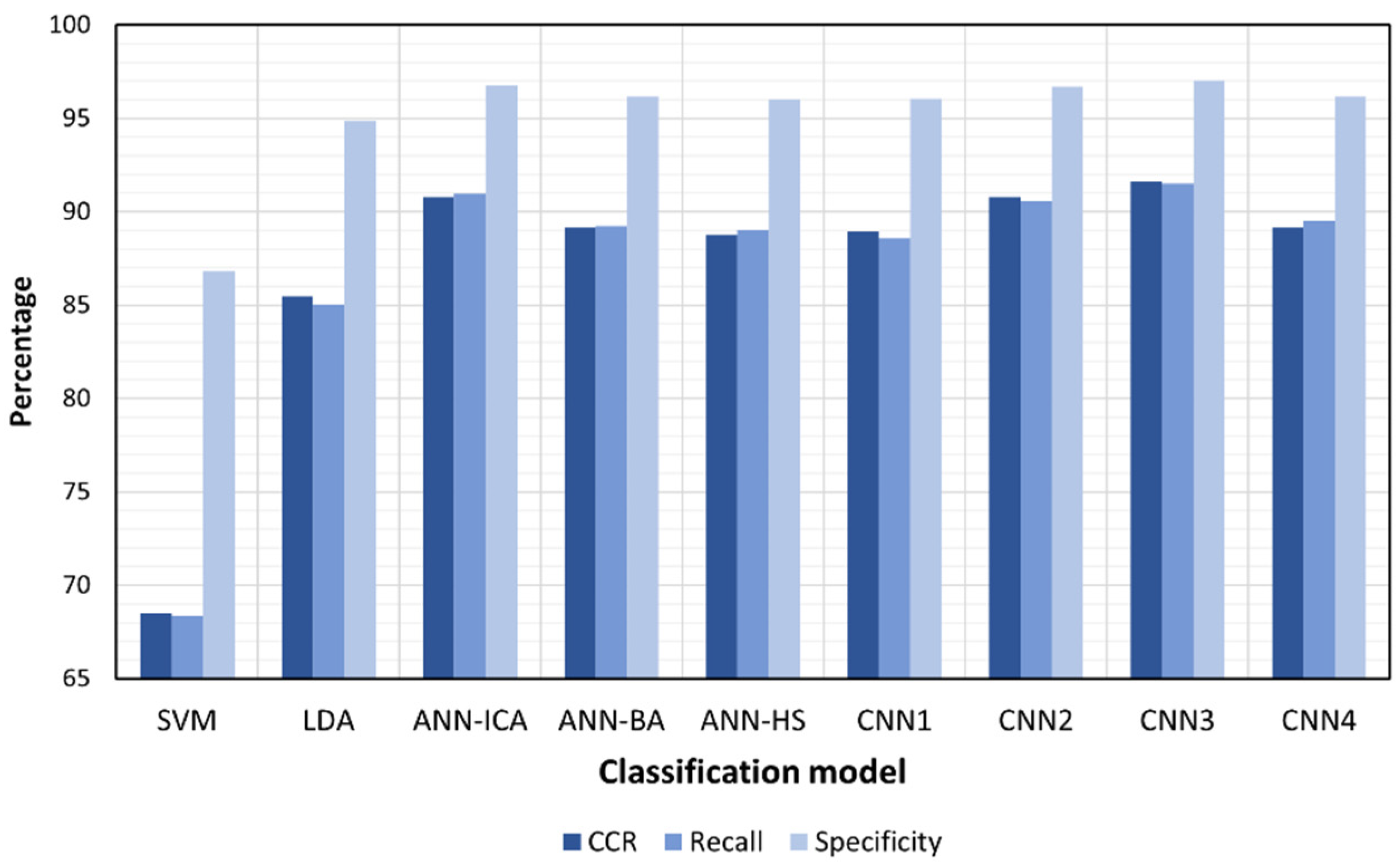
For a better comparison of the classifiers, Figure 4 presents the correct classification rate (CCR) and the average recall and specificity of all the studied classifiers.
In general, the experimental results of this study show that hyperspectral imaging is a feasible technique to detect the excessive use of nitrogen in tomato leaves at an early stage. The best methods are able to achieve an average classification accuracy for the four classes above 90%. Still, there is room for improvement and future research should be applied before the practical application of these techniques under outdoor and remote sensing conditions. The main findings of the present research are the following:
  • Three diverse classification approaches were compared in the present study using classic machine learning methods, hybrid combinations of artificial neural networks and metaheuristic algorithms and convolutional neural networks. The last two approaches have clearly shown their superiority over the classic methods, which only achieved below 86% classification accuracy. However, the correct design of the structure of the neural networks (both in ANN and in CNN) is essential to obtain precise results. The differences between structures can produce changes around 3% in the classification rate, for example, from 88.9% for CNN1 to 91.6% for CNN3. Therefore, our experiments show that recent approaches based on deep learning, and especially CNNs, should be preferred for similar problems of hyperspectral image analysis. However, future research should pay special attention to the correct design of the networks since an inadequate architecture could produce poor results. In any case, other machine learning techniques based on ANN would be preferred in applications that require low computational cost, such as the implementation of the system in mobile devices or embedded systems.
  • Regarding the comparison of the four CNN structures designed, it can be observed that as the number of convolution layers increases (CNN1, CNN2 and CNN3) the accuracy of the system also increases (88.9%, 90.8% and 91.6%, respectively). However, after the limit of six layers, the result of the classifier drops to 89.2% for CNN4. It can be deduced that a higher number of layers is not always better to obtain a better classification accuracy. Moreover, the number of parameters for this network is near two million, which requires more computational cost and more information to correctly train the network parameters.
  • The obtained results show that it is feasible to detect the application of nitrogen overdose even after the first day. This would enable the farmers to apply early corrective measures to avoid future problems in the plants. Moreover, the detection of excess nitrogen is very high for the first day (class B) with only a 2.5% error for CNN3. Since the fertilizer is applied with irrigation water, it is quickly absorbed by the plants, allowing an early detection on the leaves. In the CNN3 classifier, only one sample of class A was misclassified as class D, and the specificity of class D was 100%, which means that when the system predicted D, it was always correct. Additionally, if we considered a binary classification problem, i.e., normal (class A)/excessive nitrogen (classes B, C and D), the accuracy of CNN3 would be 95.3%. These are very promising values for the practical feasibility of the method. In order to improve the precision, a real use of the system could involve testing several leaves for each plant, making the method more robust to individual misclassifications.
  • Although we can find in the literature many works related to the estimation of nitrogen content in plant leaves using hyperspectral images and machine learning methods, almost all of them deal with regression problems. For example, Yu et al. [35] proposed stacked auto-encoders and fully connected neural networks on oilseed rape leaf, achieving a coefficient of determination (R2) of 0.903; Corti et al. [36] applied partial least square regression models on a spinach canopy with an R2 of 0.83; Zhang et al. [37] used a multivariate linear regression model on corn leaves obtaining an R2 of 0.750; Miphokasap and Wannasiri [38] analyzed the application of support vector regression on a sugarcane canopy, resulting in an R2 of 0.78; and Ye et al. [39] achieved R2 values between 0.772 and 0.784 with partial least squares regression and multiple linear regression on apple leaves. All these cases estimated the nitrogen content with hyperspectral images. However, in our case, the purpose is not directly to produce an estimation of the amount of nitrogen but to detect an incorrect application of nitrogen fertilizer in the plants. For this reason, we deal with a classification problem of nitrogen treatment, instead of a regression case. In general, it can be observed that the most advanced models based on deep learning and convolutional neural networks are able to obtain the best results. Nevertheless, these results cannot be directly compared since they use different types of plants, capturing devices, experimental conditions and, ultimately, different datasets.
  • Finally, as already mentioned, there are several aspects that should be considered in future research for the application of this technique in a remote sensing scenario when the images are captured by drones or satellites. First, the system should include a leaf detection algorithm to obtain the information only from the leaves or from the areas of large vegetative content. Second, the effect of natural illumination, clouds, shadows, etc., on the spectra should also be studied for the wavelengths of interest in the visible and near-infrared ranges. Alternatively, a new structure of 3D CNN could be used considering two spatial dimensions and one spectral dimension, which would be able to learn the spatial and spectral relations. This model should be able to jointly detect the leaves and the nitrogen excess, although this would require new field work and experiments. For example, attention mechanisms could be used to center the attention of the network in the space and the spectra of interest.

4. Conclusions

In this study, a new method for the detection of nitrogen excess in the leaves of Royal tomato variety using a non-destructive hyperspectral imaging technique was presented. We evaluated and compared the performance of nine machine learning classifiers in classifying the hyperspectral information of leaf images at different wavelengths from 400 to 1100 nm, which were taken from different treatments with normal nitrogen content, and after 1, 2 and 3 days of 30% nitrogen fertilizer overdose.
The methods used for comparison included two classic machine learning techniques, namely, linear discriminant analysis (LDA) and support vector machines (SVMs), three hybrid approaches of artificial neural networks and independent component analysis (ANN-ICA), harmony search (ANN-HS) and bees algorithm (ANN-BA) and four architectures of convolutional neural networks (CNNs) with an increasing number of convolutional layers. The results indicated that the best average prediction accuracy with a correct classification rate (CCR) of 91.6% was achieved by the proposed CNN classifier with six convolutional layers. The worst results correspond to the classic methods, LDA and SVM, with a CCR of only 85.5% and 68.5%, respectively. The rest of the methods (ANN-ICA, ANN-HS, ANN-BA and the other CNNs) reached similar results ranging from 88.8% to 90.8%.
These results can be used in the development of new systems for the detection of the excessive use of fertilizers using remote sensing technology. For this purpose, new challenges should be faced in future research, such as the segmentation of leaf areas in the images and studying the effect of natural light when the images are captured by remote hyperspectral imaging technology.

Author Contributions

Conceptualization, B.B., R.P. and S.S.; methodology, R.P., S.S., R.F.-B. and G.G.-M.; software, B.B. and S.S.; validation, R.P., S.S., R.F.-B. and G.G.-M.; investigation, B.B., R.P., S.S., R.F.-B., G.G.-M. and J.M.M.-M.; resources, R.P. and S.S.; data curation, B.B., R.P. and S.S.; writing—original draft preparation, B.B. and S.S.; writing—review and editing, R.P., S.S. and G.G.-M.; visualization, R.F-B.; supervision, R.F.-B., G.G.-M. and J.M.M.-M. All authors have read and agreed to the published version of the manuscript.

Funding

This research received no external funding.

Data Availability Statement

Data used in this study are available upon reasonable request to the authors.

Conflicts of Interest

The authors declare no conflict of interest.

References

  1. Sainju, U.M.; Dris, R.; Singh, B. Mineral nutrition of tomato. Food Agric. Environ 2003, 1, 176–183. [Google Scholar]
  2. Di Cesare, L.F.; Migliori, C.; Viscardi, D.; Parisi, M. Quality of tomato fertilized with nitrogen and phosphorous. Ital. J. Food Sci. 2010, 22, 186–191. [Google Scholar]
  3. Zheng, Y.; Ma, Y.; Liu, W.; Qiu, F. Chapter 4—Plant nutrition and physiological disorders in fruit crops. In Fruit Crops; Srivastava, A.K., Hu, C., Eds.; Elsevier: Amsterdam, Netherlands, 2020; pp. 47–58. [Google Scholar] [CrossRef]
  4. García-Berná, J.A.; Ouhbi, S.; Benmouna, B.; García-Mateos, G.; Fernández-Alemán, J.L.; Molina-Martínez, J.M. Systematic mapping study on remote sensing in agriculture. Appl. Sci. 2020, 10, 3456. [Google Scholar] [CrossRef]
  5. Pantazi, X.E.; Moshou, D.; Tamouridou, A. Automated leaf disease detection in different crop species through image features analysis and One Class Classifiers. Comput. Electron. Agric. 2019, 156, 96–104. [Google Scholar] [CrossRef]
  6. Agarwal, M.; Gupta, S.; Biswas, K. A new Conv2D model with modified ReLU activation function for identification of disease type and severity in cucumber plant. Sustain. Comput. Inform. Syst. 2021, 30, 100473. [Google Scholar] [CrossRef]
  7. Agarwal, M.; Gupta, S.; Biswas, K. Development of Efficient CNN model for Tomato crop disease identification. Sustain. Comput. Inform. Syst. 2020, 28, 100407. [Google Scholar] [CrossRef]
  8. Omran, E. Early sensing of peanut leaf spot using spectroscopy and thermal imaging. Arch. Agron. Soil Sci. 2017, 63, 883–896. [Google Scholar] [CrossRef]
  9. Pourdarbani, P.; Sabzi, S.; Kalantari, D.; Arribas, J. Non-destructive visible and short-wave near-infrared spectroscopic data estimation of various physicochemical properties of Fuji apple (Malus pumila) fruits at different maturation stages. Chemom. Intell. Lab. Syst. 2020, 206, 104147. [Google Scholar] [CrossRef]
  10. Pantazi, X.E.; Moshou, D.; Oberti, R.; West, J.; Mouazen, A.M.; Bochtis, D. Detection of biotic and abiotic stresses in crops by using hierarchical self-organizing classifiers. Precis. Agric. 2017, 18, 383–393. [Google Scholar] [CrossRef]
  11. Gamon, J.A.; Somers, B.; Malenovský, Z.; Middleton, E.M.; Rascher, U.; Schaepman, M. Assessing Vegetation Function with Imaging Spectroscopy. Surv. Geophys. 2019, 40, 489–513. [Google Scholar] [CrossRef] [Green Version]
  12. Pätzold, S.; Leenen, M.; Frizen, P.; Heggemann, T.; Wagner, P.; Rodionov, A. Predicting plant available phosphorus using infrared spectroscopy with consideration for future mobile sensing applications in precision farming. Precis. Agric. 2020, 21, 737–761. [Google Scholar] [CrossRef]
  13. Jun, S.; Xin, Z.; Xiaohong, W.; Bing, L.; Chunxia, D.; Jifeng, S. Research and analysis of cadmium residue in tomato leaves based on WT-LSSVR and Vis-NIR hyperspectral imaging. Spectrochim. Acta Part A Mol. Biomol. Spectrosc. 2019, 212, 215–221. [Google Scholar] [CrossRef] [PubMed]
  14. Pan, T.T.; Chyngyz, E.; Sun, D.W.; Paliwal, J.; Pu, H. Pathogenetic process monitoring and early detection of pear black spot disease caused by Alternaria alternata using hyperspectral imaging. Postharvest Biol. Technol. 2019, 154, 96–104. [Google Scholar] [CrossRef]
  15. Yu, K.; Fang, S.; Zhao, Y. Heavy metal Hg stress detection in tobacco plant using hyperspectral sensing and data-driven machine learning methods. Spectrochim. Acta Part A Mol. Biomol. Spectrosc. 2021, 245, 118917. [Google Scholar] [CrossRef] [PubMed]
  16. Xia, J.A.; Cao, H.; Yang, Y.; Zhang, W.; Wan, Q.; Xu, L.; Ge, D.; Zhang, W.; Ke, Y.; Huang, B. Detection of waterlogging stress based on hyperspectral images of oilseed rape leaves (Brassica napus L.). Comput. Electron. Agric. 2019, 159, 59–68. [Google Scholar] [CrossRef]
  17. Xu, Y.; Du, B.; Zhang, L. Beyond the patchwise classification: Spectral-spatial fully convolutional networks for hyperspectral image classification. IEEE Trans. Big Data 2019, 6, 492–506. [Google Scholar] [CrossRef]
  18. Gu, Q.; Sheng, L.; Zhang, T.; Lu, Y.; Zhang, Z.; Zheng, K.; Hu, H.; Zhou, H. Early detection of tomato spotted wilt virus infection in tobacco using the hyperspectral imaging technique and machine learning algorithms. Comput. Electron. Agric. 2019, 167, 105066. [Google Scholar] [CrossRef]
  19. Yuan, L.; Yan, P.; Han, W.; Huang, Y.; Wang, B.; Zhang, J.; Zhang, H.; Bao, Z. Detection of anthracnose in tea plants based on hyperspectral imaging. Comput. Electron. Agric. 2019, 167, 105039. [Google Scholar] [CrossRef]
  20. Xu, Y.; Du, B.; Zhang, L. Robust Self-Ensembling Network for Hyperspectral Image Classification; IEEE Transactions on Neural Networks and Learning Systems; IEEE: Manhattan, NY, USA, 2022. [Google Scholar] [CrossRef]
  21. Rossel, R.A.V. Software for chemometric analysis of spectroscopic data. Chemom. Intell. Lab. Syst. 2018, 90, 72–83. [Google Scholar] [CrossRef]
  22. Shorten, C.; Khoshgoftaar, T.M. A survey on image data augmentation for deep learning. J. Big Data 2019, 6, 1–48. [Google Scholar] [CrossRef]
  23. Majumdar, P.; Dey, S.; Bardhan, S.; Mitra, S. Support Vector Machines for the Classification of Remote Sensing Images: A Review. In Synergistic Interaction of Big Data with Cloud Computing for Industry 4.0; CRC Press: Boca Raton, FL, USA, 2022; pp. 175–180. [Google Scholar]
  24. Fradkin, D.; Muchnik, I. Support Vector Machines for Classification. DIMACS Ser. Discret. Math. Theor. Comput. Sci. 2006, 70, 13–20. [Google Scholar]
  25. Abdi, H. Discriminant Correspondence Analysis; SAGE: Thousand Oaks, CA, USA, 2007; pp. 270–275. [Google Scholar]
  26. Sabzi, S.; Pourdarbani, R.; Arribas, J.I. A Computer Vision System for the Automatic Classification of Five Varieties of Tree Leaf Images. Computers 2020, 9, 6. [Google Scholar] [CrossRef] [Green Version]
  27. Pourdarbani, R.; Sabzi, S.; García-Amicis, V.M.; García-Mateos, G.; Molina-Martínez, J.M.; Ruiz-Canales, A. Automatic classification of chickpea varieties using computer vision techniques. Agronomy 2019, 9, 672. [Google Scholar] [CrossRef] [Green Version]
  28. Pham, D.T.; Castellani, M. The bees algorithm: Modelling foraging behaviour to solve continuous optimization problems. Proc. Inst. Mech. Eng. Part C J. Mech. Eng. Sci. 2009, 223, 2919–2938. [Google Scholar] [CrossRef]
  29. Atashpaz-Gargari, E.; Lucas, C. Imperialist Competitive Algorithm: An Algorithm for Optimization Inspired by Imperialistic Competition. In Proceedings of the 2007 IEEE Congress on Evolutionary Computation, Singapore, 25–28 September 2007; pp. 4661–4667. [Google Scholar]
  30. Ragav, V.; Li, B. Convolutional Neural Networks in Visual Computing: A Concise Guide; CRC Press: Boca Raton, FL, USA, 2017; ISBN 978-1-351-65032-8. [Google Scholar]
  31. LeCun, Y.; Bottou, L.; Bengio, Y.; Haffner, P. Gradient-based learning applied to document recognition. Proc. IEEE 1998, 86, 2278–2324. [Google Scholar] [CrossRef] [Green Version]
  32. Krizhevsky, A.; Sutskever, I.; Hinton, G.E. Imagenet classification with deep convolutional neural networks. Commun. ACM 2017, 60, 84–90. [Google Scholar] [CrossRef] [Green Version]
  33. Simonyan, K.; Zisserman, A. Very deep convolutional networks for large-scale image recognition. arXiv 2014, arXiv:1409.1556. [Google Scholar]
  34. Sabzi, S.; Pourdarbani, R.; Rohban, M.H.; García-Mateos, G.; Paliwal, J.; Molina-Martínez, J.M. Early detection of excess nitrogen consumption in cucumber plants using hyperspectral imaging based on hybrid neural networks and the imperialist competitive algorithm. Agronomy 2021, 11, 575. [Google Scholar] [CrossRef]
  35. Yu, X.; Lu, H.; Liu, Q. Deep-learning-based regression model and hyperspectral imaging for rapid detection of nitrogen concentration in oilseed rape (Brassica napus L.) leaf. Chemom. Intell. Lab. Syst. 2018, 172, 188–193. [Google Scholar] [CrossRef]
  36. Corti, M.; Gallina, P.M.; Cavalli, D.; Cabassi, G. Hyperspectral imaging of spinach canopy under combined water and nitrogen stress to estimate biomass, water, and nitrogen content. Biosyst. Eng. 2017, 158, 38–50. [Google Scholar] [CrossRef]
  37. Zhang, N.; Li, P.C.; Liu, H.; Huang, T.C.; Liu, H.; Kong, Y.; Dong, Z.C.; Yuan, Y.H.; Zhao, L.L.; Li, J.H. Water and nitrogen in-situ imaging detection in live corn leaves using near-infrared camera and interference filter. Plant Methods 2021, 17, 1–11. [Google Scholar] [CrossRef] [PubMed]
  38. Miphokasap, P.; Wannasiri, W. Estimations of Nitrogen Concentration in Sugarcane Using Hyperspectral Imagery. Sustainability 2018, 10, 1266. [Google Scholar] [CrossRef]
  39. Ye, X.; Abe, S.; Zhang, S. Estimation and mapping of nitrogen content in apple trees at leaf and canopy levels using hyperspectral imaging. Precis. Agric. 2020, 21, 198–225. [Google Scholar] [CrossRef]
Figure 1. System description showing the different stages in early identification of nitrogen-rich tomato plants by hyperspectral imaging.
Remotesensing 14 06366 g001
Figure 2. Some examples of RGB images of the tomato plants prepared for hyperspectral imaging. (a,b) Sample views of the tomato pots. (cf) Sample tomato leaves after 0 (class A), 1 (class B), 2 (class C) and 3 (class D) days in nitrogen overdose treatment, respectively.
Remotesensing 14 06366 g002
Figure 3. Images of some tomato leaves captured using hyperspectral imaging on days (AD), at different wavelengths.
Remotesensing 14 06366 g003
Figure 4. Comparison of the correct classification rate (CCR), and the average recall and specificity for the four classes obtained by the nine methods for nitrogen treatment classification.
Remotesensing 14 06366 g004
Table 1. Optimal configuration of the neural network parameters set by ANN-HS. Satlins: symmetric saturating linear transfer function. Radbas: radial basis transfer function. Softmax: softmax transfer function. Trainlm: Levenberg–Marquardt backpropagation. Learnwh: Widrow–Hoff weight/bias learning function.
DescriptionOptimal Values
Number of hidden layers3
Number of neurons per layer1st layer: 9; 2nd layer: 17; 3rd layer: 23
Transfer functions per layerSatlins, radbas, softmax
Backpropagation network training functionTrainlm
Weight/bias learning functionLearnwh
Table 2. Optimal configuration of the neural network parameters set by ANN-BA. Purelin: linear transfer function. Tansig: hyperbolic tangent sigmoid transfer function. Logsig: log-sigmoid transfer function. Trainscg: scaled conjugate gradient backpropagation. Learnk: Kohonen weight learning function.
DescriptionOptimal Values
Number of hidden layers3
Number of neurons per layer1st layer: 13; 2nd layer: 21; 3rd layer: 25
Transfer functions per layerPurelin, tansig, logsig
Backpropagation network training functionTrainscg
Weight/bias learning functionLearnk
Table 3. Optimal configuration of the neural network parameters set by ANN-ICA. Radbas: radial basis transfer function. Tansig: hyperbolic tangent sigmoid transfer function. Trainrp: resilient backpropagation. Learngd: gradient descent weight and bias learning function.
DescriptionOptimal Values
Number of hidden layers2
Number of neurons per layer1st layer: 19; 2nd layer: 12
Transfer functions per layerRadbas, tansig
Backpropagation network training functionTrainrp
Weight/bias learning functionLearngd
Table 4. Description of the first convolutional neural network (CNN1) for the classification of the nitrogen excess class in tomato leaves.
Layer (Type)Output ShapeNumber of Parameters
conv1d_1 (Conv1D)(316, 32)256
max_pooling1d (MaxPooling)(158, 32)0
conv1d_2 (Conv1D)(156, 64)6208
max_pooling1d_1 (MaxPooling)(78, 64)0
conv1d_3 (Conv1D)(76, 128)24,704
flatten (Flatten)(9728)0
dense (Dense)(4)38,916
Total params: 70,084, trainable params: 70,084 and non-trainable params: 0.
Table 5. Description of the second convolutional neural network (CNN2) for the classification of the nitrogen excess class in tomato leaves.
Layer (Type)Output ShapeNumber of Parameters
conv1d_1 (Conv1D)(316, 32)256
max_pooling1d_1 (MaxPooling)(158, 32)0
conv1d_2 (Conv1D)(154, 64)10,304
max_pooling1d_2 (MaxPooling)(77, 64)0
conv1d_3 (Conv1D)(73, 128)41,088
max_pooling1d_3 (MaxPooling)(36, 128)0
conv1d_4 (Conv1D)(34, 256)98,560
max_pooling1d_4 (MaxPooling)(17, 256)0
conv1d_5 (Conv1D)(15, 512)393,728
flatten (Flatten)(7680)0
dense (Dense)(4)30,724
Total params: 574,660, trainable params: 574,660 and non-trainable params: 0.
Table 6. Description of the third convolutional neural network (CNN3) for the classification of the nitrogen excess class in tomato leaves.
Layer (Type)Output ShapeNumber of Parameters
conv1d_1 (Conv1D)(316, 64)512
max_pooling1d_1 (MaxPooling)(158, 64)0
conv1d_2 (Conv1D)(154, 128)41,088
conv1d_3 (Conv1D)(150, 128)82,048
max_pooling1d_1 (MaxPooling)(75, 128)0
conv1d_4(Conv1D)(71, 256)164,096
max_pooling1d_2 (MaxPooling)(35, 256)0
conv1d_5 (Conv1D)(31, 256)327,936
max_pooling1d_3 (MaxPooling)(15, 256)0
conv1d_6 (Conv1D)(13, 512)393,728
flatten_10 (Flatten)(6656)0
dense_10 (Dense)(4)26,628
Total params: 1,036,036, trainable params: 1,036,036 and non-trainable params: 0.
Table 7. Description of the fourth convolutional neural network (CNN4) for the classification of the nitrogen excess class in tomato leaves.
Layer (Type)Output ShapeNumber of Parameters
conv1d_1 (Conv1D)(316, 64)512
max_pooling1d_1 (MaxPooling)(158, 64)0
conv1d_2 (Conv1D)(154, 128)41,088
conv1d_3 (Conv1D)(150, 128)82,048
max_pooling1d_1 (MaxPooling)(75, 128)0
conv1d_4 (Conv1D)(71, 256)164,096
conv1d_5 (Conv1D)(67, 256)327,936
max_pooling1d_2 (MaxPooling)(33, 256)0
conv1d_6 (Conv1D)(31, 512)393,728
max_pooling1d_3 (MaxPooling)(15, 512)0
conv1d_7 (Conv1D)(13, 512)786,944
flatten (Flatten)(6656)0
dense (Dense)(4)26,628
Total params: 1,822,980, trainable params: 1,822,980 and non-trainable params: 0.
Table 8. SVM classifier performance using the confusion matrix, the classification error per class, the area under the ROC curve (AUC) and the correct classification rate (CCR).
ClassABCDTotal DataMisclassified (%)AUCCCR (%)
A59737911289.830.71968.50
B1114511216.140.919
C202288913957.950.725
D129227411758.110.790
Table 9. Performance evaluation of SVM classifier for classes A, B, C and D using different criteria.
ClassRecallAccuracySpecificityFP-RatePrecisionF-Score
A52.6779.5789.3210.6764.1357.84
B94.2188.1585.3214.677583.51
C63.3074.4479.4220.5757.8960.48
D63.2484.3893.216.7979.5670.47
Table 10. LDA classifier performance using the confusion matrix, the classification error per class, the area under the ROC curve (AUC) and the correct classification rate (CCR).
ClassABCDTotal DataMisclassified (%)AUCCCR (%)
A74034411251.350.92085.48
B1112801218.040.995
C150124013912.100.942
D5041081178.330.977
Table 11. Performance evaluation of LDA classifier for classes A, B, C and D using different criteria.
ClassRecallAccuracySpecificityFP-RatePrecisionF-Score
A66.0787.6394.245.7577.8971.49
B92.5697.89100010096.13
C89.2087.2686.4713.5272.9480.25
D92.3096.9898.721.2796.4294.32
Table 12. ANN-ICA classifier performance using the confusion matrix, the classification error per class, the area under the ROC curve (AUC) and the correct classification rate (CCR).
ClassABCDTotal DataMisclassified (%)AUCCCR (%)
A98013111212.500.96690.79
B3113501216.610.992
C146119013914.390.972
D1201141172.560.999
Table 13. Performance evaluation of ANN-ICA classifier for classes A, B, C and D using different criteria.
ClassRecallAccuracySpecificityFP-RatePrecisionF-Score
A87.5093.2795.054.9484.4885.96
B93.3896.5297.642.3593.3893.38
C85.6192.1194.755.2486.8686.23
D97.4399.1099.690.3099.1398.27
Table 14. ANN-BA classifier performance using the confusion matrix, the classification error per class, the area under the ROC curve (AUC) and the correct classification rate (CCR).
ClassesABCDTotal DataMisclassified (%)AUCCCR (%)
A91020111223.080.95989.16
B0117401213.420.994
C148117013918.800.963
D1501111175.410.999
Table 15. Performance evaluation of ANN-BA classifier for classes A, B, C and D using different criteria.
ClassRecallAccuracySpecificityFP-RatePrecisionF-Score
A81.2592.3795.834.1685.8483.40
B96.6996.2496.083.9290.0093.22
C84.1790.4593.006.9982.9783.57
D94.8798.4199.690.3099.1096.94
Table 16. ANN-HS classifier performance using the confusion matrix, the classification error per class, the area under the ROC curve (AUC) and the correct classification rate (CCR).
ClassABCDTotal DataMisclassified (%)AUCCCR (%)
A94116111219.150.97488.75
B1112711218.040.992
C1511113013923.010.950
D1011151171.740.999
Table 17. Performance evaluation of ANN-HS classifier for classes A, B, C and D using different criteria.
ClassRecallAccuracySpecificityFP-RatePrecisionF-Score
A83.9292.5395.234.7684.6884.30
B92.5695.3896.403.5990.3291.42
C81.2989.6693.046.9582.4881.88
D98.2999.0899.370.6298.2998.29
Table 18. CNN classifiers performance using the confusion matrix, the classification error per class, the area under the ROC curve (AUC) and the correct classification rate (CCR).
StructureClassABCDTotal DataMisclassified
(%)
AUCCCR
(%)
A82426011236.590.965
1B1115501215.220.99488.95
C6512801398.590.969
D2231101176.360.999
A87915111228.740.985
2B0117401213.420.98290.79
C3912701399.450.981
D1211131173.540.999
A96412011216.700.981
3B0118301212.540.98991.61
C6612701399.450.977
D1541071179.350.995
A10036311212.000.985
4B31099012111.010.99289.16
C215113013923.010.978
D0121141172.630.996
Table 19. Performance evaluation of the four CNN classifiers for classes A, B, C and D using different criteria.
StructureClassRecallAccuracySpecificityFP-RatePrecisionF-Score
A73.2191.7797.512.4890.1080.78
1B95.0496.2396.673.3291.2693.11
C92.0890.6290.029.9779.0185.04
D94.0198.41100010096.91
A77.6793.8698.891.1095.60485.71
2B96.6994.8794.235.7685.4090.69
C91.3693.2794.065.9386.3988.81
D96.5898.8899.690.3099.1297.83
A85.7195.1198.051.9493.2089.30
3B97.5296.1395.654.3488.7292.91
C91.3693.5294.415.5886.9889.12
D91.4597.81100010095.53
A89.2892.3793.336.6080.6484.74
4B90.0895.4097.322.6792.3791.21
C81.2991.0295.005.0086.9284.01
D97.4398.6499.070.9097.4397.43
Publisher’s Note: MDPI stays neutral with regard to jurisdictional claims in published maps and institutional affiliations.