
A Method for Retrieving Cloud-Top Height Based on a Machine Learning Model Using the Himawari-8 Combined with Near Infrared Data


Abstract
:1. Introduction
2. Method
2.1. Data
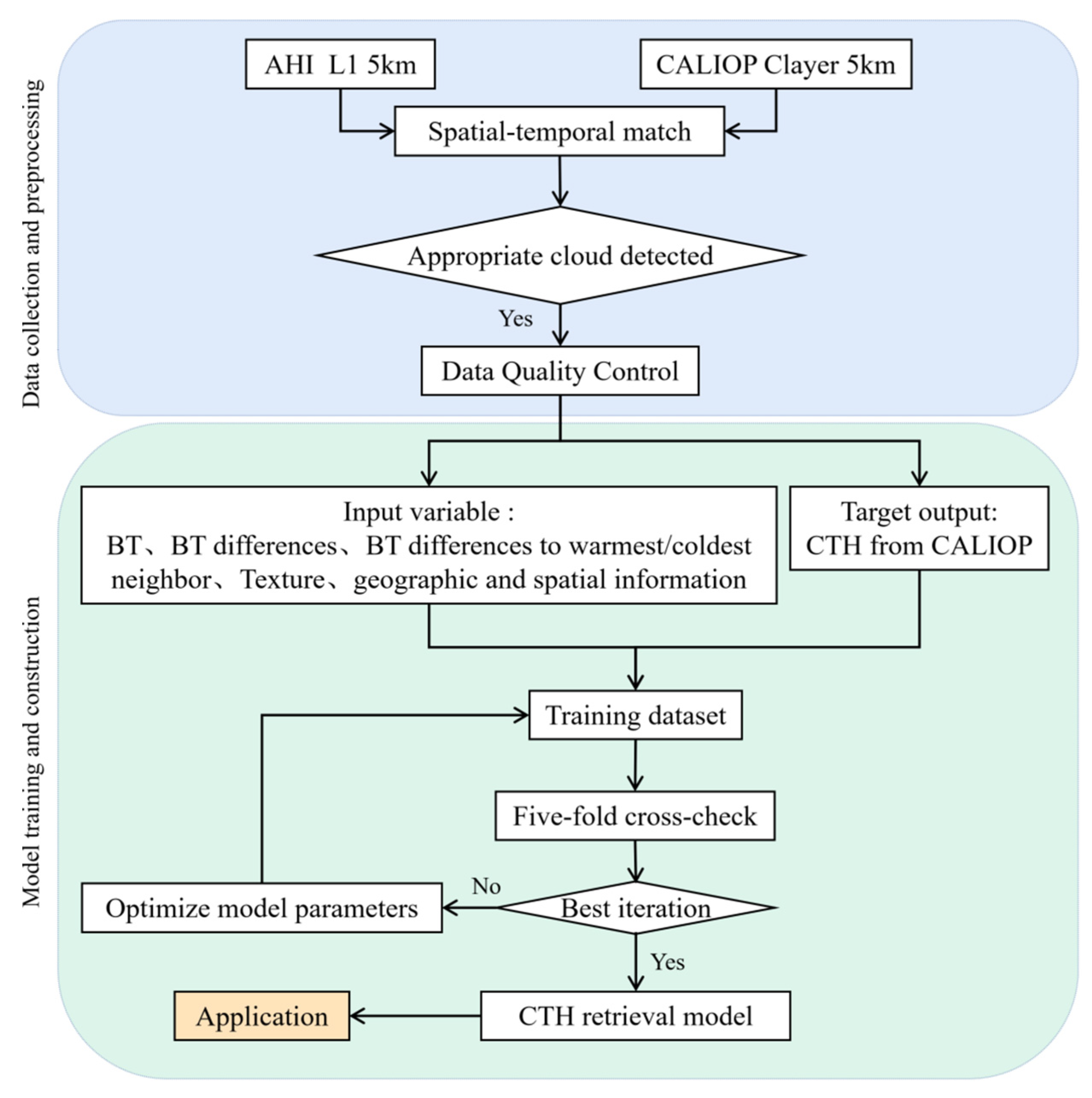
2.2. Retrieval Algorithm
2.3. Model Input Parameters
2.4. Model Training Method
3. Result
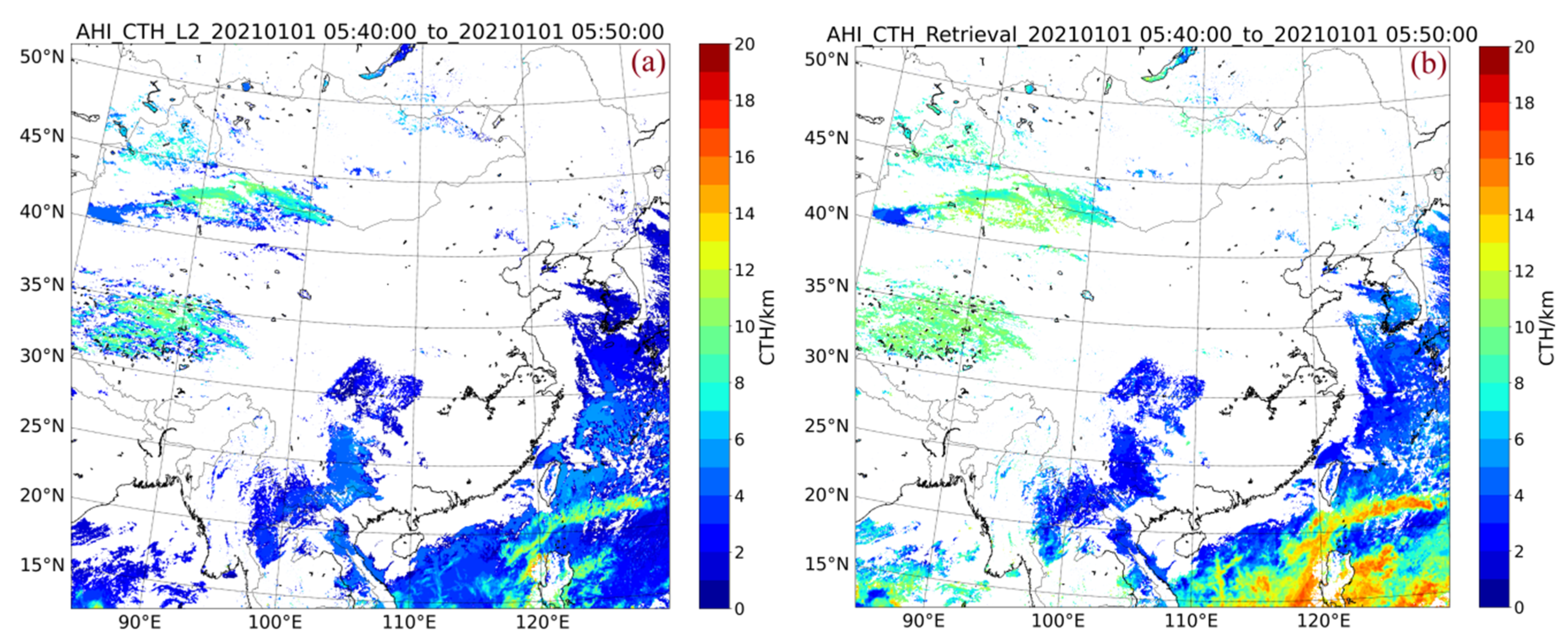
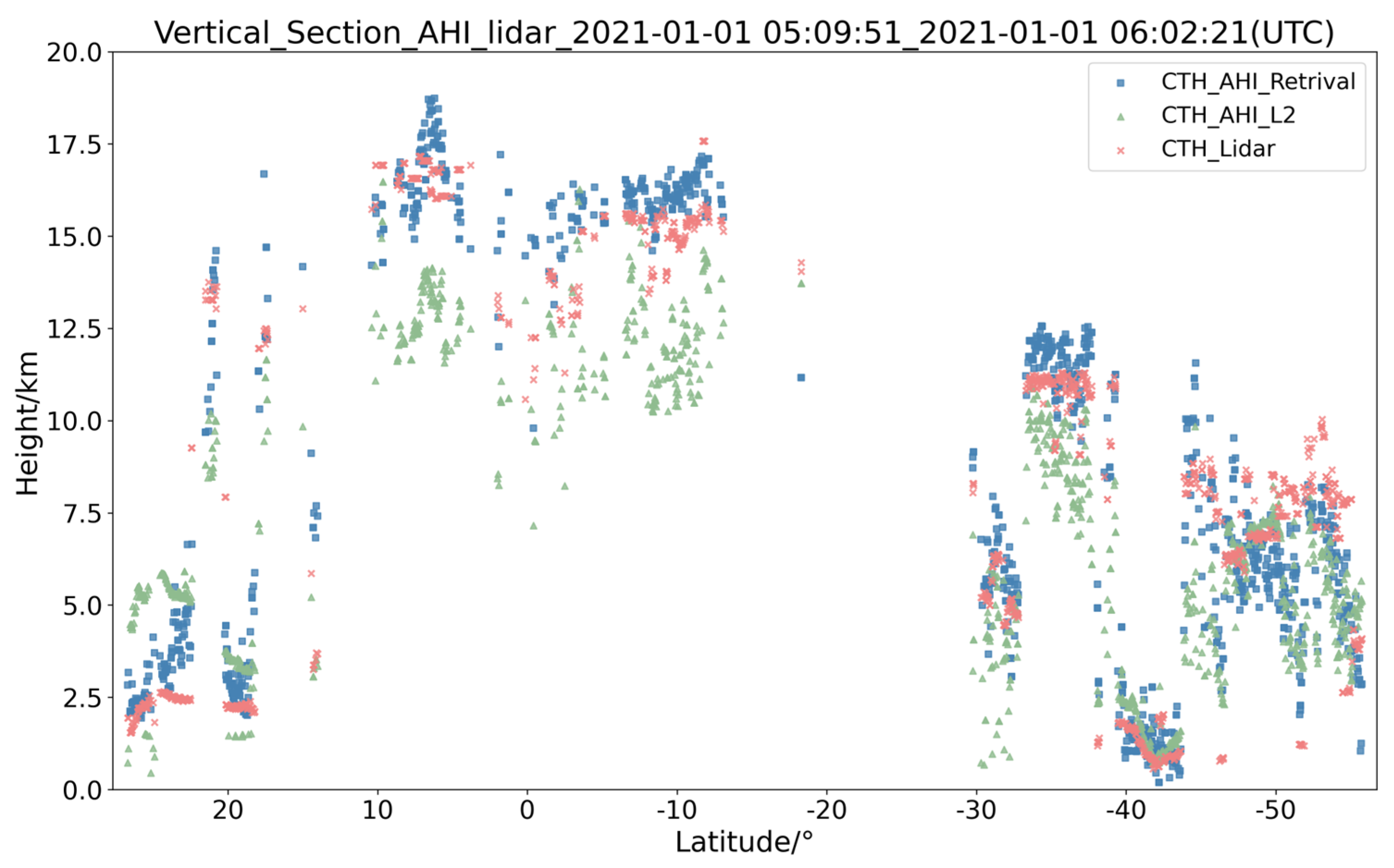
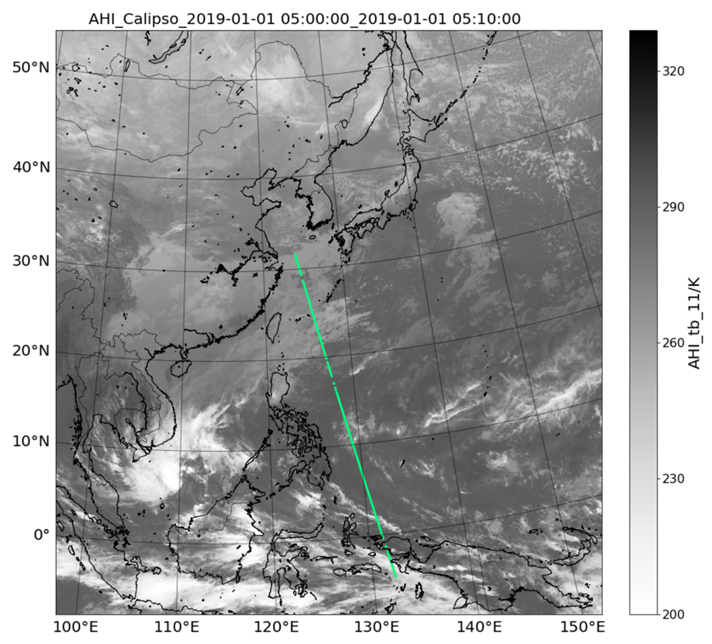
3.1. Case Analysis
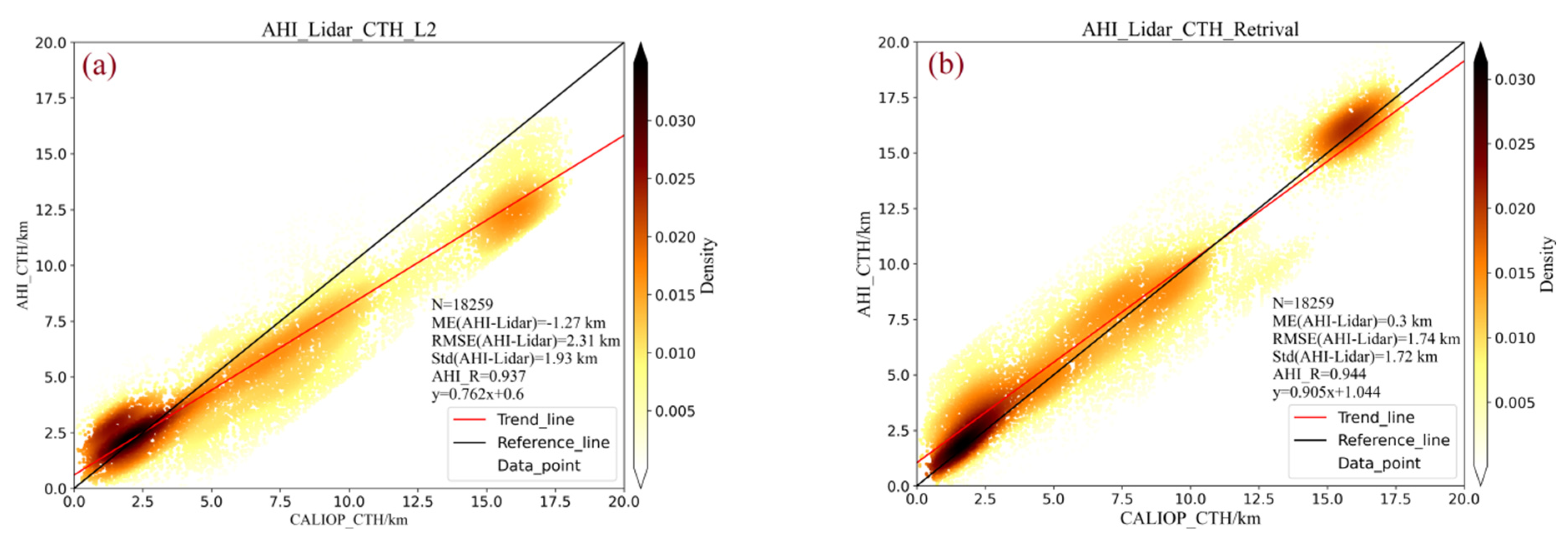
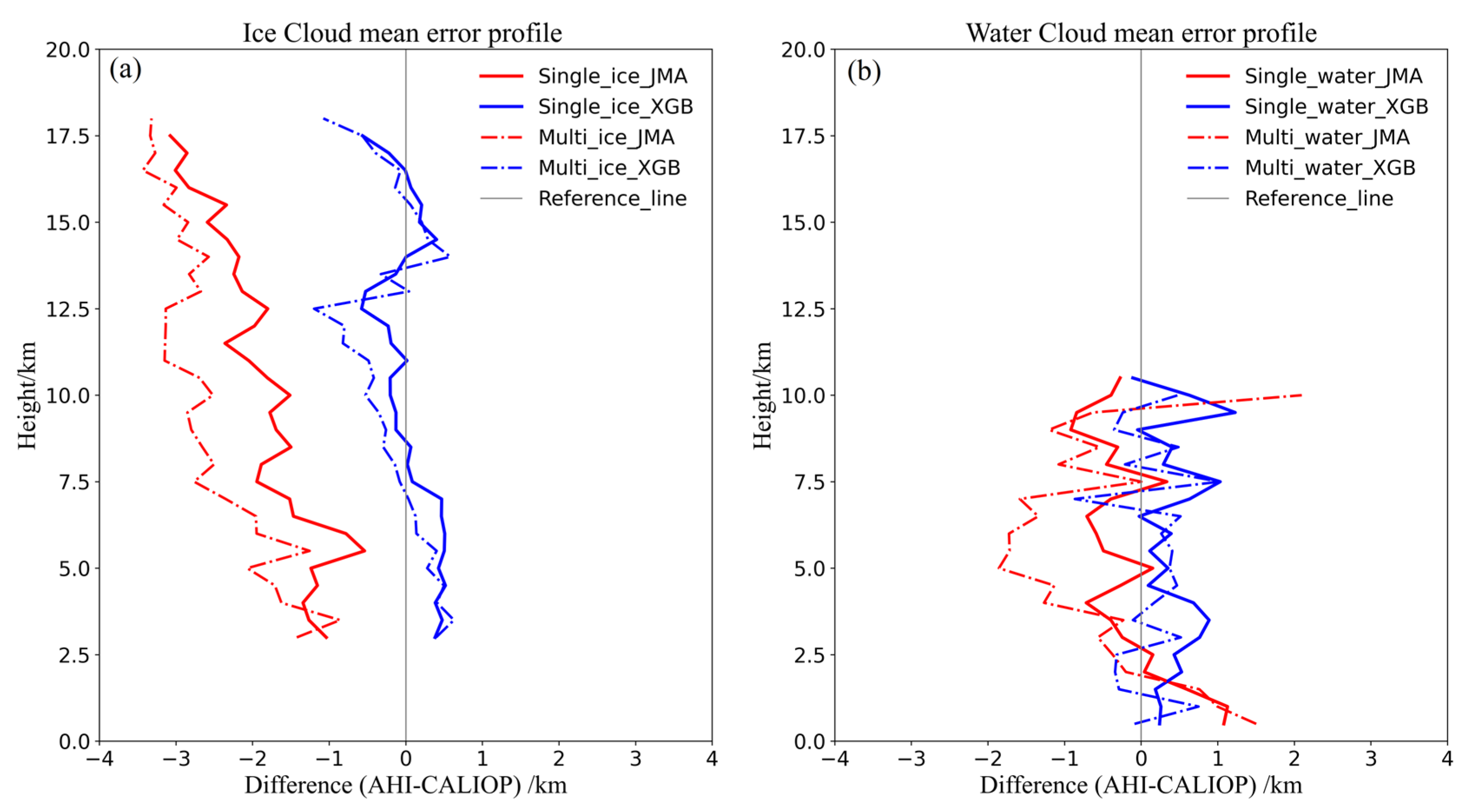
3.2. Statistic Analysis
4. Discussion
5. Conclusions
Author Contributions
Funding
Data Availability Statement
Acknowledgments
Conflicts of Interest
References
- Stephens, G.L.; Webster, P.J. Clouds and climate: Sensitivity of simple systems. J. Atmos. Sci. 1981, 38, 235–247. [Google Scholar] [CrossRef]
- Sassen, K.; Wang, Z.; Liu, D. Global distribution of cirrus clouds from CloudSat/Cloud-Aerosol lidar and infrared pathfinder satellite observations (CALIPSO) measurements. J. Geophys. Res. Atmos. 2008, 113. [Google Scholar] [CrossRef]
- Wang, H.; Su, W. Evaluating and understanding top of the atmosphere cloud radiative effects in Intergovernmental Panel on Climate Change (IPCC) Fifth Assessment Report (AR5) Coupled Model Intercomparison Project Phase 5 (CMIP5) models using satellite observations. J. Geophys. Res. Atmos. 2013, 118, 683–699. [Google Scholar] [CrossRef] [Green Version]
- Li, J.; Yi, Y.; Minnis, P.; Huang, J.; Yan, H.; Ma, Y.; Wang, W.; Ayers, J.K. Radiative Effect Differences between Multi-layered and Single-layer Clouds Derived from CERES.CALIPSO, and CloudSat Data. J. Quant. Spectrosc. Radiat. Transfer. 2011, 112, 361–375. [Google Scholar] [CrossRef]
- Boucher, O.; Randall, D.; Artaxo, P.; Bretherton, C.; Feingold, G.; Forster, P.; Zhang, X.Y. Clouds and Aerosols. In Climate Change 2013: The Physical Science Basis. Contribution of Working Group I to the Fifth Assessment Report of the Intergovernmental Panel on Climate Change; Cambridge University Press: Cambridge, UK, 2013. [Google Scholar]
- Holz, R.E.; Ackerman, S.A.; Nagle, F.W.; Frey, R.; Dutcher, S.; Kuehn, R.E.; Vaughan, M.; Baum, B.A. Global Moderate resolution Imaging Spectroradiometer (MODIS)cloud detection and height evaluation using CALIOP. J. Geophys. Res. Atmos. 2008, 113, 1–17. [Google Scholar] [CrossRef] [Green Version]
- Miller, S.D.; Forsythe, J.M.; Partain, P.T.; Haynes, J.M.; Bankert, R.L.; Sengupta, M.; Mitrescu, C.; Hawkins, J.D.; Vonder, H.; Thomas, H. Estimating Three-dimensional Cloud Structure via Statistically Blended Satellite Observations. J. Appl. Meteorol. Clim. 2014, 53, 437–455. [Google Scholar] [CrossRef] [Green Version]
- Hollars, S.; Qiang, F.; Comstock, J.; Ackerman, T. Comparison of cloud-top height retrievals from ground-based 35 GHz MMCR and GMS-5 satellite observations at ARM TWP Manus site. Atmos. Res. 2004, 72, 169–186. [Google Scholar] [CrossRef]
- Platnick, S.; King, M.D.; Ackerman, S.A.; Menzel, W.P.; Baum, B.A.; Riédi, J.C.; Frey, R.A. The MODIS cloud products: Algorithms and examples from Terra. IEEE Trans Geosci Remote Sens. 2003, 41, 459–473. [Google Scholar] [CrossRef] [Green Version]
- Minnis, P.; Sun-Mack, S.; Young, D.F.; Heck, P.W.; Garber, D.P.; Chen, Y.; Spangenberg, D.A.; Arduini, R.F.; Trepte, Q.Z.; Smith, W.L.; et al. CERES Edition-2 Cloud Property Retrievals Using TRMM VIRS and Terra and Aqua MODIS Data—Part I: Algorithms. IEEE Trans. Geosci. Remote Sens. 2011, 49, 4374–4400. [Google Scholar] [CrossRef]
- Campbell, J.R.; Dolinar, E.K.; Lolli, S.; Fochesatto, G.J.; Gu, Y.; Lewis, J.R.; Marquis, J.W.; McHardy, T.M.; Ryglicki, D.R.; Welton, E.J. Cirrus Cloud Top-of-the-Atmosphere Net Daytime Forcing in the Alaskan Subarctic from Ground-Based MPLNET Monitoring. J. Appl. Meteorol. Clim. 2020, 60, 51–63. [Google Scholar] [CrossRef]
- Da, C. Preliminary assessment of the Advanced Himawari Imager (AHI) measurement onboard Himawari-8 geostationary satellite. Remote Sens. Lett. 2015, 6, 637–646. [Google Scholar] [CrossRef]
- Liu, Q.; Li, Y.; Yu, M.; Long, S.C.; Yang, C. Daytime Rainy Cloud Detection and Convective Precipitation Delineation Based on a Deep Neural Network Method Using GOES-16 ABI Images. Remote Sens. 2019, 11, 2555. [Google Scholar] [CrossRef] [Green Version]
- Min, M.; Wu, C.; Li, C.; Liu, H.; Xu, N.; Wu, X.; Chen, L.; Wang, F.; Sun, F.; Qin, D.; et al. Developing the Science Product Algorithm Testbed for Chinese Next-Generation Geostationary Meteorological Satellites: Fengyun-4 Series. J. Meteorol. Res. 2017, 31, 708–719. [Google Scholar] [CrossRef]
- Heidinger, A.K.; Bearson, N.; Foster, M.J.; Li, Y.; Wanzong, S.; Ackerman, S.; Holz, R.E.; Platnick, S.; Meyer, K. Using Sounder Data to Improve Cirrus Cloud Height Estimation from Satellite Imagers. J. Atmos. Ocean. Technol. 2019, 36, 1331–1342. [Google Scholar] [CrossRef]
- Heidinger, A.K.; Pavolonis, M.J. Gazing at Cirrus Clouds for 25 Years through a Split Window. Part I: Methodology. J. Appl. Meteorol. Clim. 2009, 48, 6. [Google Scholar] [CrossRef]
- Li, J.; Menzel, W.P.; Schreiner, A.J. Variational Retrieval of Cloud Parameters from GOES Sounder Longwave Cloudy Radiance Measurements. J. Appl. Meteorol. 2001, 40, 312–330. [Google Scholar] [CrossRef]
- Tan, Z.; Ma, S.; Zhao, X.; Yan, W.; Lu, W. Evaluation of Cloud Top Height Retrievals from China’s Next-Generation Geostationary Meteorological Satellite FY-4A. J. Meteorol. Res. 2019, 33, 553–562. [Google Scholar] [CrossRef]
- Iwabuchi, H.; Putri, N.S.; Saito, M.; Tokoro, Y.; Sekiguchi, M.; Yang, P.; Baum, B.A. Cloud property retrieval from multiband infrared measurements by Himawari-8. J. Meteorol. Soc. Jpn. 2018, 96B, 27–42. [Google Scholar] [CrossRef] [Green Version]
- Heidinger, A. ABI cloud height. In NOAA/NESDIS/STAR, GOES-R Algorithm Theoretical Basis Document (ATBD); NOAA NESDIS Center for Satellite Applications and Research: College Park, MD, USA, 2012; pp. 1–77. [Google Scholar]
- Schmit, T.J.; Gunshor, M.M.; Menzel, W.P.; Gurka, J.J.; Li, J.; Bachmeier, A.S. Introducing the next generation Advanced Baseline Imager on GOES-R. Bull. Am. Meteorol. Soc. 2005, 86, 1079–1096. [Google Scholar] [CrossRef]
- Menzel, W.P.; Frey, R.A.; Zhang, H.; Wylie, D.P.; Moeller, C.C.; Holz, R.; Maddux, B.; Baum, B.A.; Strabala, K.I.; Gumley, L.E. MODIS global cloud-top pressure andamountestimation: Algorithm description and results. J. Appl. Meteorol. Clim. 2008, 47, 1175–1198. [Google Scholar] [CrossRef]
- Li, J.; Yi, Y.H.; Stamnes, K.; Ding, X.D.; Wang, T.H.; Jin, H.C.; Wang, S.S. A new approach to retrieve cloud base height of marine boundary layer clouds. Geophys. Res. Lett. 2013, 40, 4448–4453. [Google Scholar] [CrossRef]
- Li, J.; Li, Z.; Wang, P.; Schmit, T.J.; Bai, W.; Atlas, R. An efficient radiative transfermodel for hyperspectral IR radiance simulation and applications under cloudy skyconditions. J. Geophys. Res. Atmos. 2017, 122, 7600–7613. [Google Scholar] [CrossRef]
- Baum, B.; Menzel, W.P.; Frey, R.; Tobin, D.; Holz, R.; Ackerman, S. MODIS cloudtop property refinements for Collection 6. J. Appl. Meteorol. Clim. 2012, 51, 1145–1163. [Google Scholar] [CrossRef]
- Weisz, E.; Li, J.; Menzel, W.P.; Heidinger, A.K.; Kahn, B.H.; Liu, C.Y. Comparison ofAIRS.MODIS.CloudSat and CALIPSO cloud top height retrievals. Geophys. Res. Lett. 2007, 34, 1–5. [Google Scholar] [CrossRef]
- Sherwood, S.C.; Chae, J.-H.; Minnis, P.; McGill, M. Underestimation of deep convective cloud tops by thermal imagery. Geophys. Res. Lett. 2004, 31, 11. [Google Scholar] [CrossRef] [Green Version]
- Min, M.; Li, J.; Wang, F.; Liu, Z.J.; Menzel, W.P. Retrieval of cloud top properties from advanced geostationary satellite imager measurements based on machine learning algorithms. Remote Sens. Environ. 2019, 239, 111616. [Google Scholar] [CrossRef]
- Chang, F.L.; Minnis, P.; Ayers, J.K.; McGill, M.J.; Palikonda, R.; Spangenberg, D.A.; Smith, W.L., Jr.; Yost, C.R. Evaluation of satellite-based upper troposphere cloud top height retrievals in multilayer cloud conditions during TC4. J. Geophys. Res. Atmos. 2010, 10, 11–15. [Google Scholar] [CrossRef]
- Chang, F.L.; Minnis, P.; Bing, L.; Khaiyer, M.M.; Palikonda, R.; Spangenberg, D.A. A modified method for inferring upper troposphere cloud top height using the GOES 12 imager 10.7 and 13.3 μm data. J. Geophys. Res. Atmos. 2010, 115, 1–13. [Google Scholar] [CrossRef] [Green Version]
- Key, J.R.; Intrieri, J.M. Cloud Particle Phase Determination with the AVHRR. J. Appl. Meteorol. 2000, 39, 1797–1804. [Google Scholar] [CrossRef]
- Daniel, J.S. Cloud liquid water and ice measurements from spectrally resolved near-infrared observations: A new technique. J. Geophys. Res. Atmos. 2002, 107, 1–16. [Google Scholar] [CrossRef]
- Palmer, K.F.; Williams, D. Optical properties of water in the near infrared*. J. Opt. Soc. Am. B (1917-1983) 1974, 64, 1107–1110. [Google Scholar] [CrossRef]
- Pilewskie, P.; Twomey, S. Cloud Phase Discrimination by Reflectance Measurements near 1.6 and 2.2 µm. J. Atmos. Sci. 1987, 44, 3419–3420. [Google Scholar] [CrossRef]
- Min, M.; Bai, C.; Guo, J.; Sun, F.; Liu, C.; Wang, F.; Xu, H.; Tang, S.; Li, B.; Di, D.; et al. Estimating summertime precipitation from Himawari-8 and global forecast system based on machine learning. IEEE Trans. Geosci. Remote Sens. 2019, 57, 2557–2570. [Google Scholar] [CrossRef]
- Tan, Z.; Huo, J.; Shuo, M.; Han, D.; Wang, X.; Hu, S.; Yan, W. Estimating cloud base height from Himawari-8 based on a random forest algorithm. Int. J. Remote Sens. 2021, 42, 2485–2501. [Google Scholar] [CrossRef]
- Håkansson, N.; Adok, C.; Thoss, A.; Scheirer, R.; Hörnquist, S. Neural network cloud top pressure and height for MODIS. Atmos. Meas. Tech. 2018, 11, 3177–3196. [Google Scholar] [CrossRef] [Green Version]
- Wang, X.; Iwabuchi, H.; Takaya, Y. Cloud identification and property retrieval from Himawari-8 infrared measurements via a deep neural network. Remote Sens. Environ. 2022, 275, 113026. [Google Scholar] [CrossRef]
- Husi, L.; Nagao, T.M.; Nakajima, T.Y.; Riedi, J.; Ishimoto, H.; Baran, A.J.; Shang, H.; Sekiguchi, M.; Kikuchi, M. Ice cloud properties from Himawari-8/AHI nextgeneration geostationary satellite: Capability of the AHI to monitor the DC cloud generation process. IEEE Trans Geosci Remote Sens. 2019, 57, 3229–3239. [Google Scholar]
- Iwabuchi, H.; Saito, M.; Tokoro, Y.; Putri, N.S.; Sekiguchi, M. Retrieval of radiative and microphysical properties of clouds from multispectral infrared measurements. Prog. Earth Planet. Sci. 2016, 3, 32. [Google Scholar] [CrossRef] [Green Version]
- Hostetler, C.A.; Liu, Z.; Reagan, J.; Vaughan, M.; Winker, D.; Osborn, M.; Hunt, W.H.; Powell, K.A.; Trepte, C. CALIOP Algorithm Theoretical Basis Document, Calibration and Level 1 Data Products. Available online: https://www-calipso.larc.nasa.gov/resources/pdfs/PC-SCI-201v1.0.pdf (accessed on 10 January 2022).
- Winker, D.M.; Vaughan, M.A.; Omar, A.; Hu, Y.; Powell, K.A.; Liu, Z.; Hunt, W.H.; Young, S.A. Overview of the CALIPSO mission and CALIOP data processing algorithms. J Atoms. Ocean. Technol. 2009, 26, 2310–2323. [Google Scholar] [CrossRef]
- Friedman, J.H. Stochastic gradient boosting. Comput. Stat. Data. An. 2002, 38, 367–378. [Google Scholar] [CrossRef]
- Chen, T.; Guestrin, C. XGBoost: A Scalable Tree Boosting System. ACM 2016, 785–794. [Google Scholar] [CrossRef]
- Romeo, L.; Frontoni, E. A Unified Hierarchical XGBoost Model for Classifying Priorities for COVID-19 Vaccination Campaign. Pattern Recogn. 2021, 121, 108197. [Google Scholar] [CrossRef] [PubMed]
- Inoue, T. On the Temperature and Effective Emissivity Determination of Semi-Transparent Cirrus Clouds by Bi-Spectral Measurements in the 10 µm Window Region. J. Meteorol. Soc. Jpn. 1985, 63, 88–99. [Google Scholar] [CrossRef] [Green Version]
- Derrien, M.; Lavanant, L.; Le, H.; Gleau. Retrieval of the cloud top temperature of semi-transparent clouds with AVHRR. In Proceedings of the IRS’88, Deepak Publ., Hampton, Lille, France, 8–24 August 1988; pp. 199–202.
- Hamada, A.; Nishi, N. Development of a Cloud-Top Height Estimation Method by Geostationary Satellite Split-Window Measurements Trained with CloudSat Data. J. Appl. Meteorol. Clim. 2010, 49, 2035–2049. [Google Scholar] [CrossRef]


| Number of Channels | Center Wavelength of the Channel | Channel Characteristics |
|---|---|---|
| Channel 05 | 1.6 µm | Low water vapor absorption channel |
| Channel 07 | 3.9 µm | Different cloud phase states have absorption differences |
| Channel 10 | 7.3 µm | Water vapor absorption channel |
| Channel 11 | 8.6 µm | |
| Channel 14 | 11.2 µm | Split window channel |
| Channel 15 | 12.3 µm | |
| Channel 16 | 13.3 µm | CO2 absorption channel |
| Variable Type | Variable | Note |
|---|---|---|
| Reflectivity | R1.6 | Sensitive to the phase state of cloud |
| Bright Temperature | BT11.2 | Temperatures close to opaque cloud |
| BT7.3 | It is important to identify high optical thin cloud | |
| BT13.3 | It is important to identify high optical thin cloud | |
| BT difference between channels | BT11.2-BT12.3, BT8.6-BT12.3, BT7.3-BT12.3, BT13.3-BT12.3 | Holds information about whether the cloud is opaque and how transparent it is |
| Texture parameters | (BT11.2)text, (BT3.9)text, (R1.6)text (BT11.2-BT12.3)text, (BT11.2-BT3.9)text | Save information about the opacity, translucency, or edges of cloud |
| BT differences to warmest/coldest neighbor | BT11.2-BT11.2 W, BT11.2-BT11.2 C, BT12.3 W-BT11.2 W, BT12.3 C-BT11.2 C, BT11.2 W-BT3.9 W, BT11.2 C-BT3.9 C | Cloud Optical Thickness |
| Geographic and spatial information | Latitude, Longitude, SZA, VZA | Eliminate some uncertainties caused by geographic location and space |
| Cloud Scene | ME/km | RMSE/km | Std/km | |||
|---|---|---|---|---|---|---|
| CTHJMA | CTHXGB | CTHJMA | CTHXGB | CTHJMA | CTHXGB | |
| Ice | −2.34 | −0.05 | 2.80 | 1.75 | 1.70 | 1.54 |
| Water | 0.82 | 0.73 | 1.67 | 1.44 | 1.51 | 1.43 |
| Mix | −1.23 | 0.34 | 2.46 | 2.00 | 2.13 | 1.97 |
| Single-layer | −0.73 | 0.56 | 1.95 | 1.72 | 1.80 | 1.62 |
| Multi-layer | −2.22 | −0.17 | 2.84 | 1.78 | 1.78 | 1.67 |
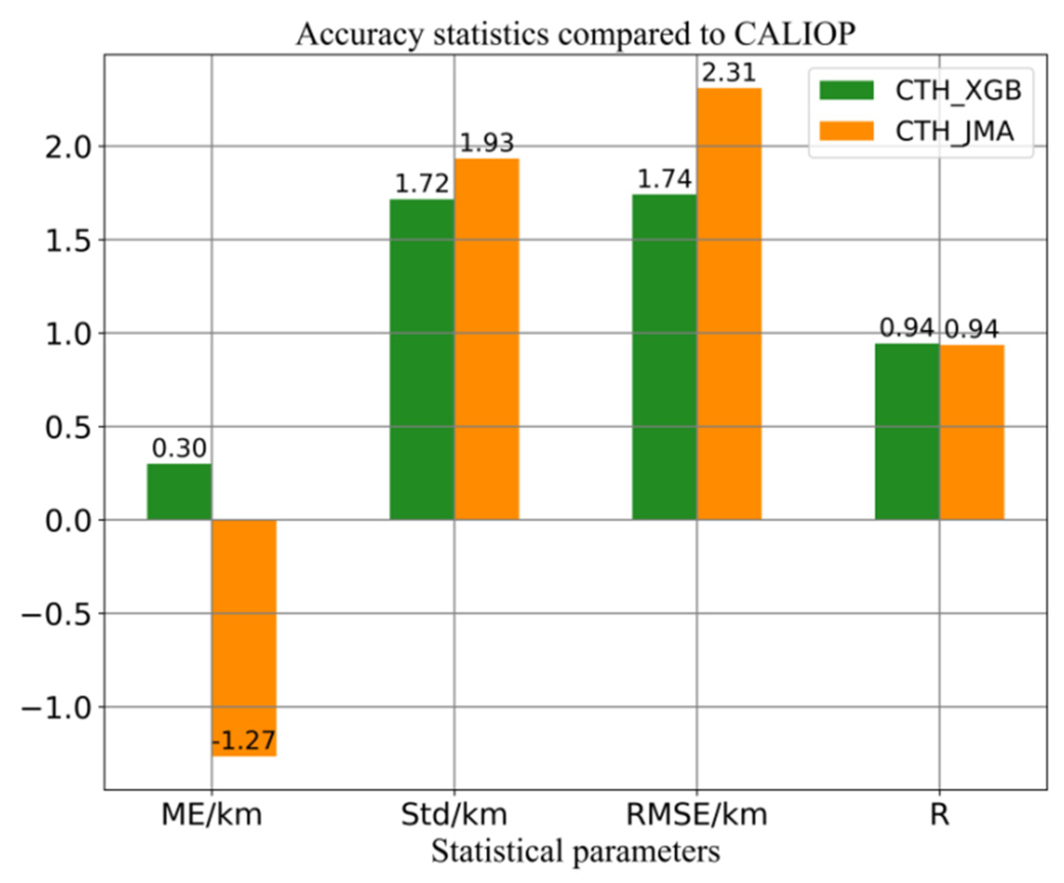
| All | −1.27 | 0.30 | 2.31 | 1.74 | 1.93 | 1.72 |
Publisher’s Note: MDPI stays neutral with regard to jurisdictional claims in published maps and institutional affiliations. |
© 2022 by the authors. Licensee MDPI, Basel, Switzerland. This article is an open access article distributed under the terms and conditions of the Creative Commons Attribution (CC BY) license (https://creativecommons.org/licenses/by/4.0/).
Share and Cite
Dong, Y.; Sun, X.; Li, Q. A Method for Retrieving Cloud-Top Height Based on a Machine Learning Model Using the Himawari-8 Combined with Near Infrared Data. Remote Sens. 2022, 14, 6367. https://doi.org/10.3390/rs14246367
Dong Y, Sun X, Li Q. A Method for Retrieving Cloud-Top Height Based on a Machine Learning Model Using the Himawari-8 Combined with Near Infrared Data. Remote Sensing. 2022; 14(24):6367. https://doi.org/10.3390/rs14246367
Chicago/Turabian StyleDong, Yan, Xuejin Sun, and Qinghui Li. 2022. "A Method for Retrieving Cloud-Top Height Based on a Machine Learning Model Using the Himawari-8 Combined with Near Infrared Data" Remote Sensing 14, no. 24: 6367. https://doi.org/10.3390/rs14246367
APA StyleDong, Y., Sun, X., & Li, Q. (2022). A Method for Retrieving Cloud-Top Height Based on a Machine Learning Model Using the Himawari-8 Combined with Near Infrared Data. Remote Sensing, 14(24), 6367. https://doi.org/10.3390/rs14246367