Global Ionospheric Total Electron Content Completion with a GAN-Based Deep Learning Framework

Abstract

The ionosphere serves as a critical medium for radio signal propagation in outer space. A good morphology of the global TEC distribution is very useful for both ionospheric studies and their relative applications. In this work, a deep learning framework was constructed for better spatial estimation in ionospheric TEC. Both the DCGAN and WGAN-GP were considered, and their performances were evaluated with spatial completion for a regional TEC. The performances were evaluated using the correlation coefficient, RMSE, and MAE. Moreover, the IAAC rapid products were used to make comparisons. The results show that both the DCGAN and WGAN-GP outperformed the IAAC CORG rapid products. The spatial TEC estimation clearly goes well with the solar activity trend. The RMSE differences had a maximum of 0.5035 TECu between the results of 2009 and 2014 for the DCGAN and a maximum of 0.9096 TECu between the results of 2009 and 2014 for the WGAN-GP. Similarly, the MAE differences had a maximum of 0.2606 TECu between the results of 2009 and 2014 for DCGAN and a maximum of 0.3683 TECu between the results of 2009 and 2014 for WGAN-GP. The performances of the CORG, DCGAN, and WGAN-GP were also verified for two selected strong geomagnetic storms in 2014 and 2017. The maximum RMSEs were 1.8354 TECu and 2.2437 TECu for the DCGAN and WGAN-GP in the geomagnetic storm on 18 February 2014, respectively, and the maximum RMSEs were 1.3282 TECu and 1.4814 TECu in the geomagnetic storm on 7 September 2017. The GAN-based framework can extract the detailed features of spatial TEC daily morphologies and the responses during geomagnetic storms.

1. Introduction

The ionosphere serves as a critical medium for radio signal propagation in outer space. In the ionosphere, there are many free electrons due to soft X-ray and far ultraviolet (UV) solar radiation as well as solar energetic particle precipitation. The coexistence of ions and electrons can lead to radio signal delay and distortion. For instance, ionospheric delay is one of the major causes of satellite navigation system error [1,2,3]. Ionization intensity is described by the total electron content (TEC) in the ionosphere. The variability in TEC can efficiently reflect the status of the ionosphere, especially during geomagnetic disturbances, and ionospheric responses can be investigated from the features of TEC. Therefore, a good morphology of the global TEC distribution is very useful for both ionospheric studies and their relative applications.

The development of global satellite navigation systems provides a good opportunity to accurately derive the TEC with dual-frequency navigation signal observables. Based on this idea, the International Global GNSS Service (IGS) has established a global TEC distribution map with a spatial resolution of 2.5° in latitude and 5° in longitude. The global TEC map is updated every two hours [4]. Currently, there are seven data analysis centers authorized by the IGS to provide global TEC products [5]. These data have a temporal span of more than twenty years, which is sufficient and solid for ionospheric studies. Compared to traditional empirical models, such as the international reference ionosphere (IRI) [6] and Nequick [7], the global TEC map is derived from global observations of more than 400 ground-based stations, and it can better reflect the real variation in the ionosphere. With this gridded map, the TEC of any location in the assumed spherical face can be interpolated. The global morphology of the ionosphere can be investigated at more detailed scales.

Short-term TEC prediction is useful for predicting the spatial–temporal variability of the ionosphere, and accurate TEC prediction can also help with the precise positioning of satellites. The Klobuchar model was widely adopted to predict short-term TEC values in the early stage, and it is the main TEC estimation and prediction tool for single-frequency GPS signals [1]. Recently, based on a well-produced global TEC map, TEC prediction has been thought to occur directly from historical time series. A few studies have revealed the feasibility of short-term TEC prediction using machine learning approaches, [8]. Recently, deep learning has been widely used for time series prediction, and given its more complicated neural network structures, it can help to increase the usage of observations with better performance [9,10,11,12,13,14]. Chen et al. (2019) constructed an R-DCGAN network to generate satisfactory ionospheric peak features with some existing ionospheric maps as additional references [15]. Chen et al. (2019) established an improved GAN structure, the regional deep convolutional GAN, to efficiently estimate the unknown part of the MIT global TEC map [16]. Ji et al. (2020) further used generative adversarial networks (GANs) to improve the IRI model for one-day regional TEC prediction [17]. Pan et al. (2020, 2021) constructed both DCGAN and SNP-GAN (spectral normalized patch GAN) frameworks to complete the MIT global TEC map, and the performance error was within 6 TECu [18,19].

These works, which are very enlightening, provide better descriptions of ionospheric TECs at different spatial scales. Considering that the current derivation of global TEC maps is entirely based on ground GNSS observations, the real accuracy is not good in those spaces above the oceans. To address this problem, spatial interpolation and estimation have been adopted to improve the TEC estimation accuracy for the ionosphere above ocean regions.

To address this problem, in this work, a deep learning framework was constructed for better spatial estimation in ionospheric TEC. Both DCGAN and WGAN-GP were considered, and the performance was evaluated with spatial completion for a regional TEC. The performance of the IGS CODR rapid product was compared with DCGAN and WGAN-GP for geomagnetically quiet and disturbed conditions.

2. Data and Methodology

2.1. Data Presentation

The original data came from the global ionosphere map (GIM) provided by the IGS final product, with a spatial resolution of 2.5° in latitude and 5° in longitude. The GIM has a total of 71 × 73 grid points. For convenient GAN framework construction, the original data were transferred to a 72 × 72 square grid. During the reformation, the data at 180°E remained in the 72nd column, and the data at 87.5°S were copied as the 72nd index. The data from 2001 to 2017 were all considered to build the corresponding training data set, and the years 2009, 2014, and 2017 were selected as test candidates. When the data in these three years were used for a test data set, they were excluded from the training data set.

IGS Ionosphere Associate Analysis Centers (IAACs) also provide a rapid GIM product for short-term GIM prediction; the prediction interval is less than 24 h. However, these rapid products generally have an average delay of 11 days. In this work, rapid GIM products from the CODE IGS data analysis center (CODR) were used to compare the performance of DCGAN and WGAN-GP. The CODR data began in 2004. In the past, the data interval was every two hours; moreover, since November 2014, the data interval was further shortened to every hour. The CODR data from 2009, 2014, and 2017 were processed in this work for the performance comparison.

2.2. Proposed Methodology

2.2.1. Construction of the DCGAN Framework

The GAN framework was first proposed by Goodfellow et al. in 2014 [20]. It is composed of two parts: the generator and discriminator. The framework trains both the generator and the discriminator. The theoretical basis of the GAN is game theory. The model training process is a competition between the generator and the discriminator. The generator uses random data to generate target data to deceive the discriminator. The discriminator improves its discrimination ability by judging the authenticity of the data generated by the generator and the real data. The two will eventually reach a state of balance. The ideal state occurs when the data generated by the generator can be confused with the real data, and the discrimination probability of the discriminator for the input real data and false data is 50%.

The training process of GAN is performed as follows: First, the generator receives random noise as input and generates false data corresponding with the size and distribution of the real data. The purpose of the generator is to generate data that cannot be distinguished by the discriminator. If the real data are represented as 1 and the false data are represented as 0, the most ideal state of the data generated occurs when the probability of the discriminator’s output is 50% false and 50% true. The discriminator is designed to discriminate the real data with an output of 1 and false data with an output of 0. During the training process, both the generator and discriminator oppose each other and are optimized; this cycle continues until the present goal is reached.

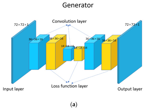
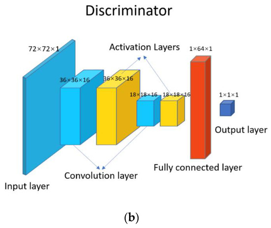
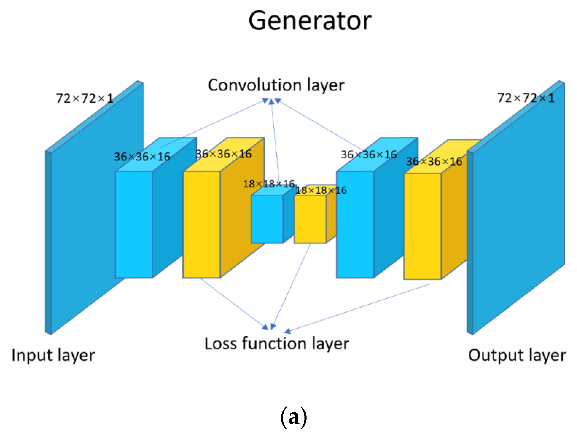
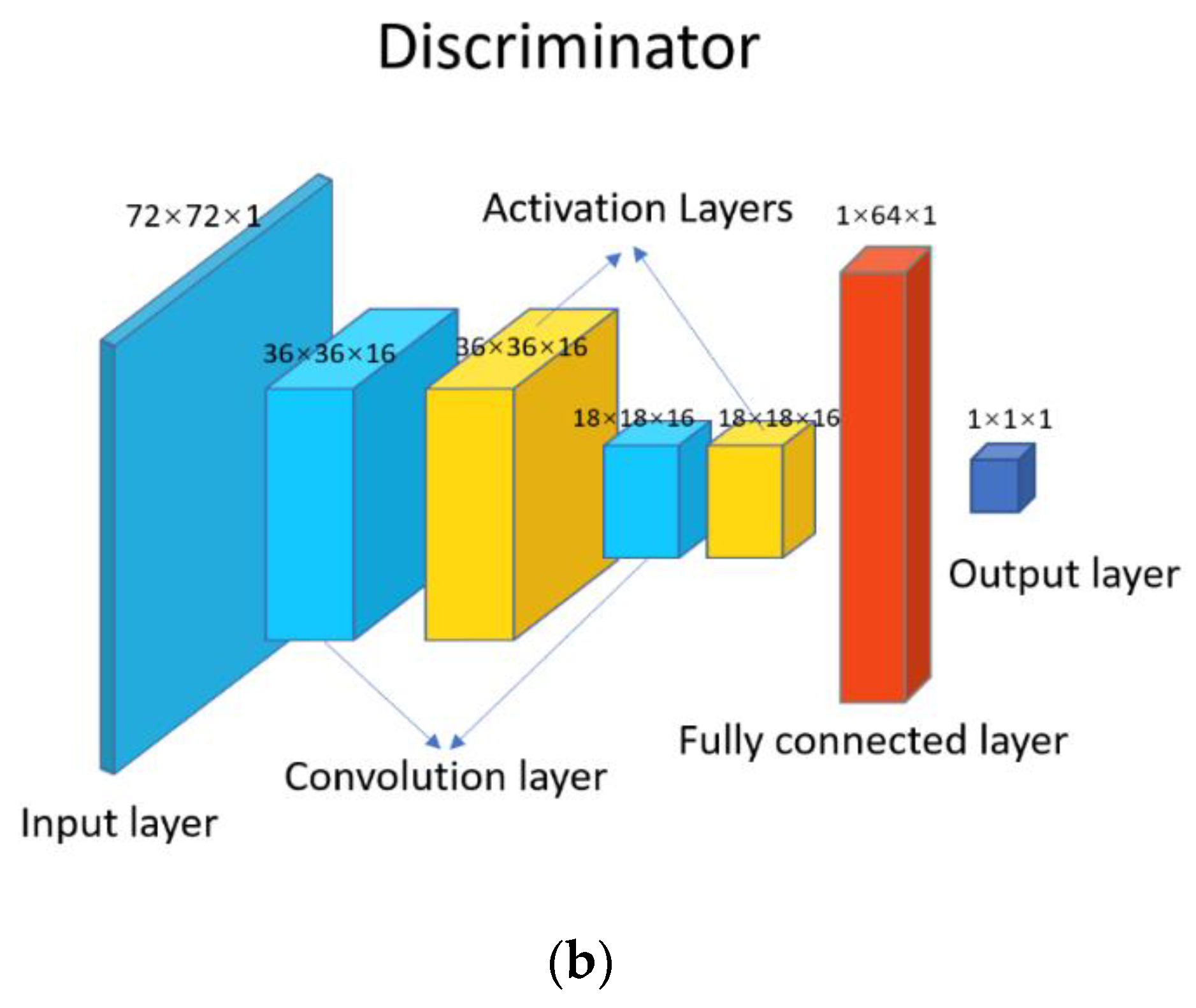
Alec Radford proposed a modified version of the GAN called the deep convolutional GAN (DCGAN) [21]. The DCGAN solves the disadvantages of unstable training and modeling in a traditional GAN, as Figure 1 demonstrated. A series of convolution and up-sampling operations are used in the generator of the DCGAN to abstract the information from random data, and new data are constructed with a false label. The discriminator in the DCGAN receives the false data from the generator and the real data and then outputs the labels for them. The loss is passed through the network of the generator to adjust the parameters for accuracy improvement. Compared to the traditional GAN, in the DCGAN, the pooling layer is replaced by step convolution to avoid information feature loss during the training process. The activation function of the generator is also modified. In addition to using $tanh\left(·\right)$ in the output layer, the ReLU function is adopted for the remaining layers. The leaky ReLU function is used for the discriminator. Meanwhile, the DCGAN improves the training speed and reduces the problem of poor initialization.

Figure 1. The proposed generator and discriminator of the DCGAN in this work.

For the generator structure of the DCGAN designed in this work, the input dimension was $18\times 18\times 1$ after the normalization process, the output dimension was $72\times 72\times 1$, and $tanh\left(·\right)$ was used as the activation function. The mechanism of the generator is to recover the global grid points in a dimension of $72\times 72$, the same dimension as the original input before downsampling. The dimension input in the discriminator was $72\times 72\times 1$, and the discriminator had two inputs: fake data from the generator and the original GIM TEC. It had one binary output to represent true or false, where 1 represented output data that were real, and 0 represented output data that were fake. Through the training process, the abilities of the generator and discriminator were both enhanced, finally making the generator infinitely output approximately real data.

2.2.2. Construction of the WGAN-GP Framework

When the traditional GAN uses Kullback–Leibler (KL) divergence and Jensen–Shannon (JS) divergence, if the generated sample distribution has no overlap with the real sample distribution, then the KL divergence is meaningless, and JS divergence becomes a constant of $log2$, which can lead to unstable generator loss when using KL divergence as the loss function of the generator. Moreover, even the gradient disappears when using JS divergence as the loss function. To solve this problem, the Wasserstein distance is used as the loss function of the discriminator [22].

The cross-entropy error is considered a loss function for the generator and discriminator in the DCGAN, while the proposed Wasserstein distance outperforms the cross-entropy error and can achieve better performance during training and testing.

The Wasserstein distance is defined as

$$W\left(P_1,P_2\right)=in{f}_{\gamma ~\prod \left(P_1,P_2\right)}{\mathsf{{\rm E}}}_{\left(x,y\right)~\gamma }\left[\Vert x-y\Vert \right]$$

(1)

where $\prod \left(P_1,P_2\right)$ is the joint distribution unit for all $P_1$ and $P_2$; for each $\gamma$, $\left(x,y\right)$ is sampled, and the distance $\Vert x-y\Vert$ under the joint distribution $\gamma$ is computed. The Wasserstein distance is defined as the bottom boundary $inf$ for the distance expectation of the samples.

Compared to KL divergence and JS divergence, the Wasserstein distance is very smooth. It can reflect the distance of two statistical distributions even if no overlap exists between the generated samples and the real samples. It can consistently provide a valuable gradient during the training process. The WGAN clips the weightings of the discriminator to satisfy the efficient computation of the Wasserstein distance, and the training performance is then constrained. To overcome this disadvantage, the modified WGAN-GP algorithm is adopted. The WGAN-GP improves the original framework of the WGAN; it retains the Wasserstein distance as part of the discriminator loss function and replaces weighting clipping with the gradient penalty. The discriminator loss function of the WGAN-GP is given as

$$L={\mathsf{{\rm E}}}_{\tilde{x}~{\mathsf{{\rm P}}}_g}\left[D\left(\tilde{x}\right)\right]-{\mathsf{{\rm E}}}_{\tilde{x}~{\mathsf{{\rm P}}}_r}\left[D\left(\tilde{x}\right)\right]+\lambda {\mathsf{{\rm E}}}_{\widehat{x}~{\mathsf{{\rm P}}}_{\widehat{x}}}\left[{\left(\Vert {\nabla }_{\widehat{x}}D{\left(\widehat{x}\right)\Vert }_2-1\right)}^2\right]$$

(2)

where $\widehat{x}$ is the interpolation between the real data and the generated data, ${\nabla }_{\widehat{x}}D\left(\widehat{x}\right)$ is the gradient for interpolation by the discriminator output, the L2 norm of ${\nabla }_{\widehat{x}}D\left(\widehat{x}\right)$ is computed, and the gradient penalty is the average difference between $\Vert {\nabla }_{\widehat{x}}D{\left(\widehat{x}\right)\Vert }_2$ and 1. The closer the gradient norm is to 1, the closer the gradient penalty and the loss of the discriminator are to 0. When the loss of the discriminator is approximately 0, it indicates equilibrium between the generator and the discriminator. In the framework of the WGAN-GP, the generator and discriminator networks are the same as those in the framework of the DCGAN.

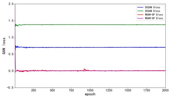
The loss variations of the generator and discriminator during the training process are presented in Figure 2. In this figure, it is shown that the losses quickly converged and tended to equilibrium; then, the game status between the generator and discriminator, which have slight fluctuations in their loss functions, was observed. In general, with increasing training epochs, the framework reached a stable state, as expected.

Figure 2. The losses of the generator and discriminator of the proposed DCGAN with increasing training epochs.

2.3. Performance Evaluation Metrics

To evaluate the performance of the proposed network, the correlation between the predicted TEC and benchmark TEC of the GIM was computed, and the root mean square error (RMSE) was used together with the correlation coefficient and mean average error (MAE) to make comparisons between different TEC prediction methods.

The computation of RMSE is given as

$$RMSE={\left\{\frac{1}{N}{\displaystyle \sum }_{n=1}^N{\left[TE{C}_{pre}-TE{C}_{gim}\right]}^2\right\}}^{1/2}$$

(3)

where $TE{C}_{pre}$ denotes the TEC prediction and the average value of the TEC prediction series, and $TE{C}_{gim}$ denotes the TEC from GIM and the average value of TEC from the GIM.

The computation of MAE is given as

$$MAE=\frac{1}{N}{\displaystyle \sum }_{n=1}^N\left|TE{C}_{pre}-TE{C}_{gim}\right|$$

(4)

The calculation of the correlation coefficient is given as

$$r\left(X,Y\right)=\frac{Cov\left(X,Y\right)}{{\sigma }_X{\sigma }_Y}$$

(5)

where $X$ and $Y$ denote the variable series for correlation, ${\sigma }_X$ and ${\sigma }_Y$ are the standard deviations of $X$ and $Y$, respectively, and $Cov\left(X,Y\right)$ denotes the covariance between $X$ and $Y$. It is also referred to as the Pearson correlation coefficient.

3. Experimental Results

In this section, the performance of the ionospheric TEC spatial estimation with the DCGAN and WGAN-GP was tested. To make a better comparison, both the solar activity and geomagnetic perturbances were considered. The data from 2001 to 2017 were selected as the training data, and the data from 2009, 2014, and 2017 were selected as the testing data. Ionospheric spatial estimation was conducted for regional verification. In particular, the value of TEC in the target region was first set to zero; then, with DCGAN and WGAN-GP, the missing TEC values, which were represented by zeros, were estimated and compared. The results were also compared with the IGS CODE rapid products (CORG).

3.1. TEC Spatial Estimation for Entire Years

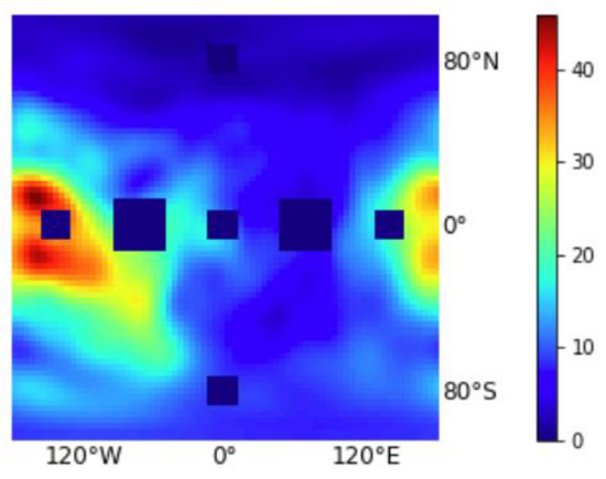
In this part, the IGS TEC values were set to zero in some selected local regions, for instance, in the ocean, where ground TEC observations are difficult to acquire. The missing TEC values were then estimated by the DCGAN and WGAN-GP. The darkened squares represent the selected regions with missing TEC values. Seven separate regions, covering high-latitude regions and the equatorial ionization anomaly region, were selected, as shown in Figure 3. These regions are located at (155°W–135°W, 5°S–5°N), (10°W–10°E, 67.5°N–77.5°N), (10°W–10°E, 5°S–5°N), (10°W–10°E, 67.5°S–77.5°S), (135°E–155°E, 5°S–5°N), (95°W–55°W, 10°S–10°N), and (45°E–85°E, 10°S–10°N). For the DCGAN and WGAN-GP, the data from 2001 to 2017 were considered as the training data and testing data. Here, three years were selected for the result presentation: testing data from 2009 (training data 2001–2008 plus 2010–2017), testing data from 2014 (training data 2001–2013 plus 2015–2017), and testing data from 2017 (training data 2001–2016).

Figure 3. Selected patterns for spatial TEC estimation.

The network frameworks for the DCGAN and WGAN-GP remained the same as above; the input dimension was $72\times 72\times 1$, and two additional convolution structures were added for the generator to maintain consistency in the dimensions during the training procedure. The well-trained models were then used to test the data from 2009, 2014, and 2017.

The correlation coefficient, root mean square error (RMSE), and mean average error between the testing methods (CODE rapid product, DCGAN, and WGAN-GP) and IGS final product were compared and demonstrated.

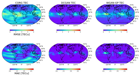
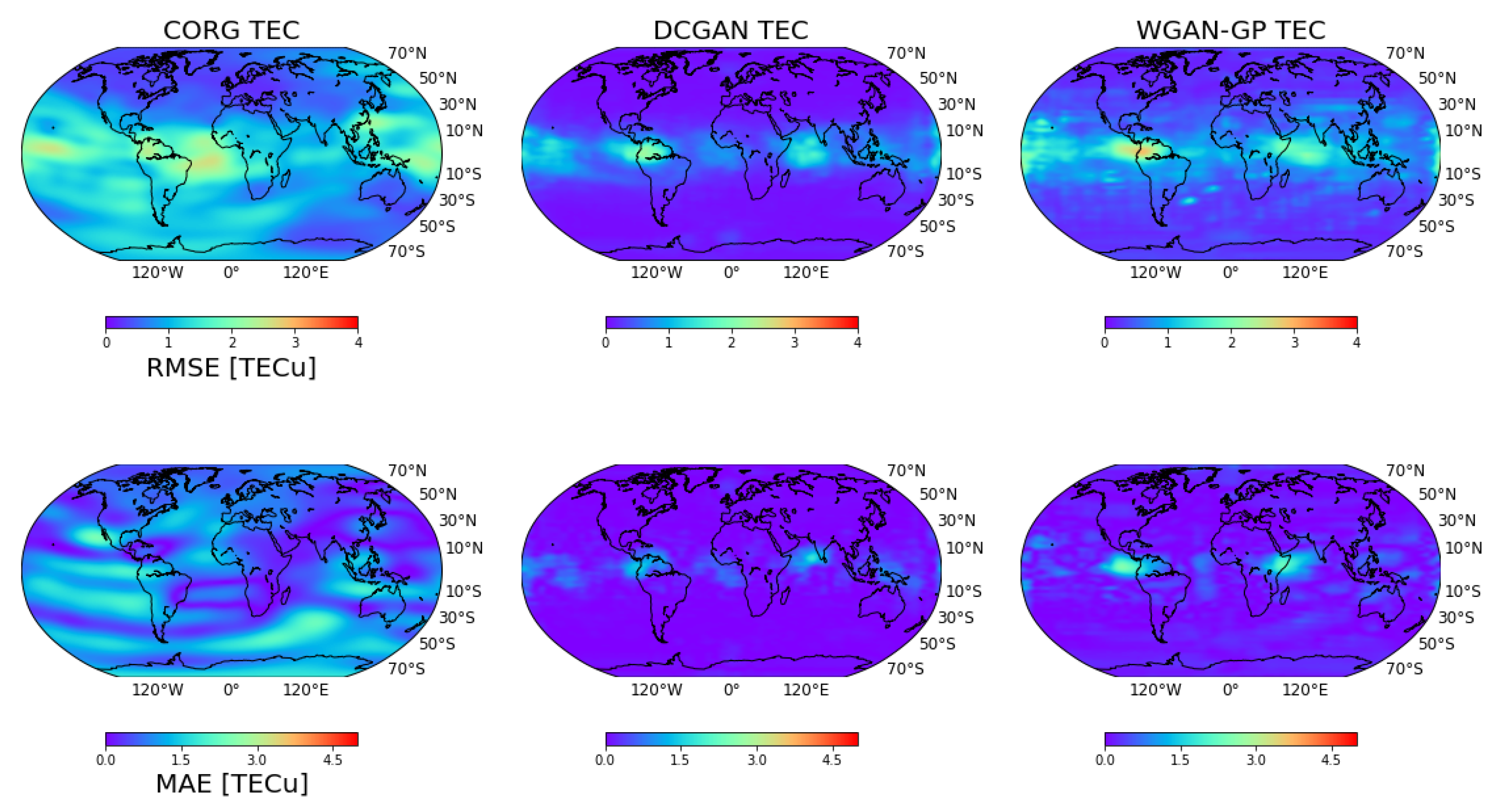
Figure 4 shows the correlation coefficient, RMSE, and MAE for the results from 2009. It is shown that both the DCGAN and WGAN-GP outperformed the CORG. For the correlation coefficient, all the results of the DCGAN and WGAN-GP exceeded 0.95; for the DCGAN, only some small parts in the equatorial ionization anomaly region were between 0.98 and 0.99; and for the remaining regions, the correlation coefficients exceeded 0.99. In the case of the WGAN-GP, in addition to some parts of the EIA region, there were small patterns in the midlatitude regions with correlation coefficients between 0.98 and 0.99. In the case of the CORG, the IGS rapid product, 82.96% correlation coefficients were larger than 0.95 in the global range. Similarly, in terms of the RMSE and MAE, the DCGAN and WGAN-GP outperformed the CORG. The DCGAN achieved better prediction accuracy than the WGAN-GP in the EIA region; the details are shown in Table 1.

Figure 4. The RMSE and MAE for spatial TEC estimation in 2009. The $71\times 73$ grids are interpolated with a spline to demonstrate a finer global feature of ionospheric TEC.

Table 1. The mean values for RMSE and MAE in 2009.

		CORG	DCGAN	WGAN-GP
RMSE (TECu)	Low	1.0672	0.5397	0.7350
	Middle	0.8803	0.1092	0.2622
	High	0.9331	0.1248	0.2426
	Global	0.9561	0.2660	0.4221
	<1 TECu	57.71%	96.70%	93.98%
MAE (TECu)	Low	0.6608	0.2641	0.2822
	Middle	0.9436	0.0529	0.0990
	High	0.9695	0.0746	0.1795
	Global	0.8528	0.1346	0.1907
	<1 TECu	64.58%	99.46%	98.38%

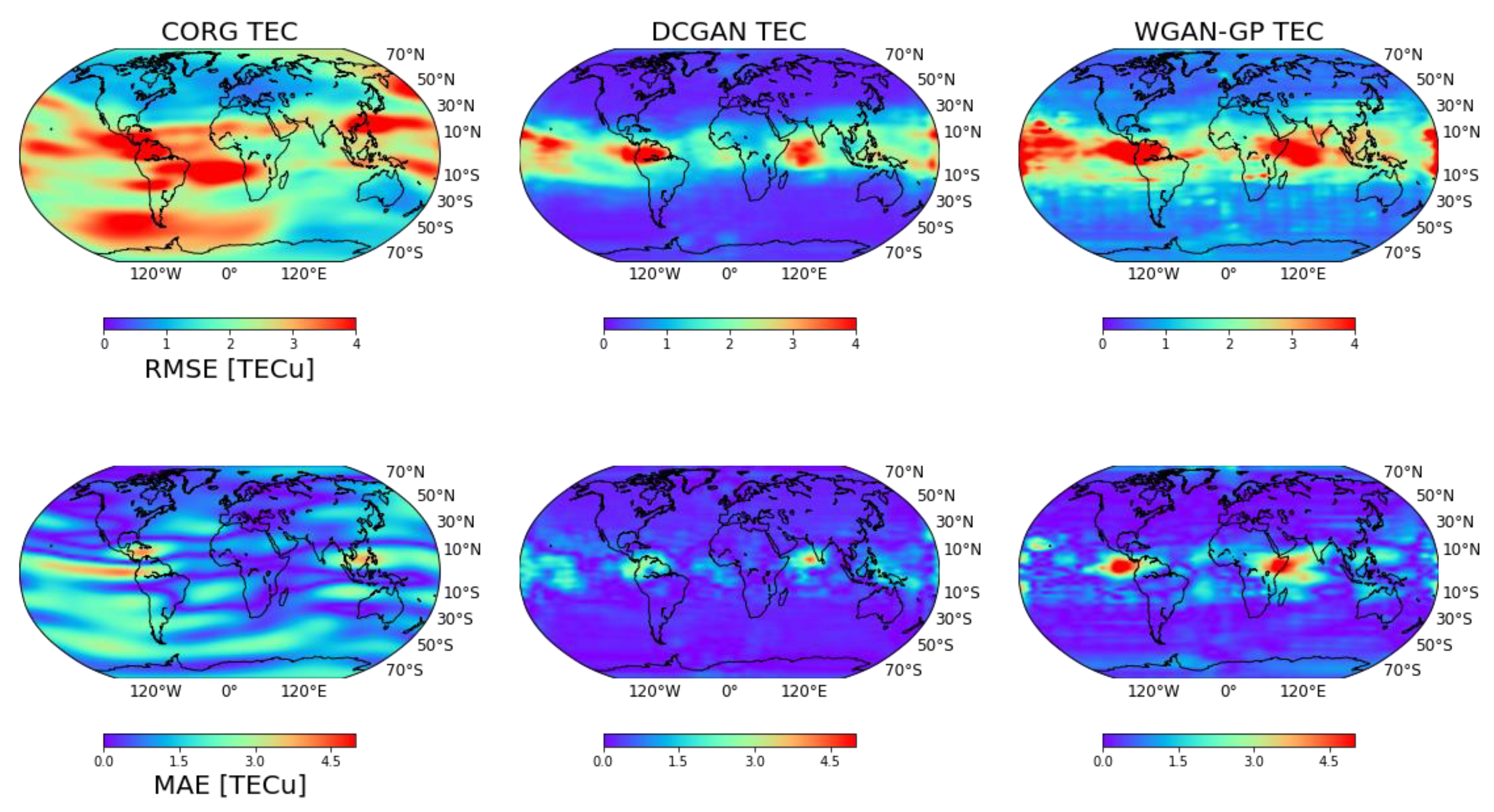
Figure 5 shows the correlation coefficient, RMSE, and MAE for the results from 2014, the solar cycle maximum in solar cycle 24. It is shown that the results of the DCGAN and WGAN-GP still outperformed those of the CORG rapid products. For the correlation coefficient, the CORG demonstrated worse performance compared to the results from 2009, as 25.39% of the regions had coefficients of less than 0.98. The performance of the DCGAN and WGAN-GP remained similar to that in 2009. For the RMSE and MAE, the DCGAN presented better accuracy compared to the WGAN-GP, but both the RMSE and MAE were larger in the EIA region compared to the results from 2009. The performance of the WGAN-GP in terms of the RMSE and MAE was less than that of the DCGAN but much better than that of the CORG, as demonstrated in Table 2.

Figure 5. The RMSE and MAE for spatial TEC estimation in 2014. The $71\times 73$ grids are interpolated with a spline to demonstrate a finer global feature of ionospheric TEC.

Table 2. The mean values for RMSE and MAE in 2014.

		CORG	DCGAN	WGAN-GP
RMSE (TECu)	Low	2.8142	1.6235	2.3564
	Middle	1.9774	0.3272	0.8638
	High	1.8438	0.2853	0.6931
	Global	2.2215	0.7695	1.3317
	<1 TECu	7.00%	74.26%	56.47%
MAE (TECu)	Low	1.2212	0.6303	0.9772
	Middle	1.1457	0.2942	0.2290
	High	1.0219	0.2429	0.4258
	Global	1.1304	0.3952	0.5590
	<1 TECu	50.07%	92.94%	85.61%

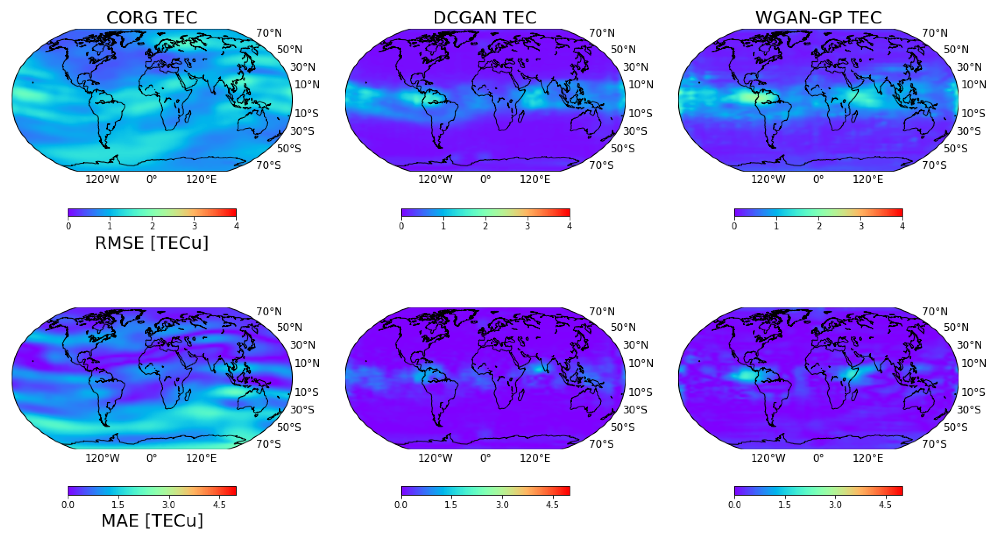
Figure 6 shows the correlation coefficient, RMSE and MAE for the results from 2017, the solar descending year of solar cycle 24. Drastic improvements in the correlation coefficients of the RMSE and MAE were observed with respect to the performance of the CORG. The correlation coefficient in 64.56% of the regions exceeded 0.98, and the global average RMSE and MAE were 1.0004 TECu and 0.8615 TECu, respectively. The RMSE was less than 1 TECu in 50.64% of the global regions, and the MAE was less than 1 TECu in 62.92% of the global regions. The performance of the DCGAN and WGAN-GP was still better than that of the CORG, as indicated in Table 3.

Figure 6. The RMSE and MAE for spatial TEC estimation in 2017. The $71\times 73$ grids are interpolated with a spline to demonstrate a finer global feature of ionospheric TEC.

Table 3. The mean values for RMSE and MAE in 2017.

		CORG	DCGAN	WGAN-GP
RMSE (TECu)	Low	1.3919	0.5501	0.8775
	Middle	0.9632	0.1214	0.3761
	High	0.7599	0.1157	0.2628
	Global	1.0004	0.2704	0.5143
	<1 TECu	50.64%	95.72%	89.81%
MAE (TECu)	Low	0.7957	0.2381	0.3276
	Middle	0.8201	0.0603	0.1243
	High	0.9690	0.0686	0.1777
	Global	0.8615	0.1257	0.2139
	<1 TECu	62.92%	99.19%	97.99%

3.2. TEC Spatial Estimation during Geomagnetic Storms

Two geomagnetic storms in 2014 and 2017 were selected to further verify the DCGAN and WGAN-GP performances. One storm occurred on 18 February 2014, and the other storm occurred on 7 September 2017.

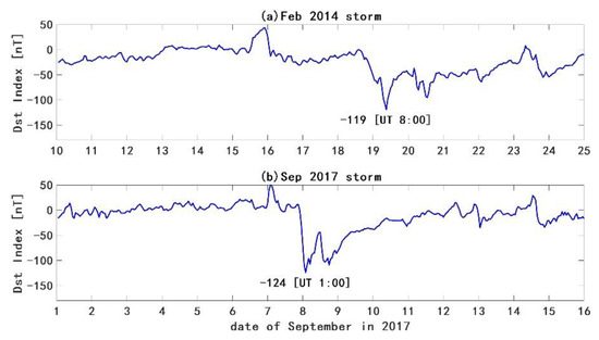
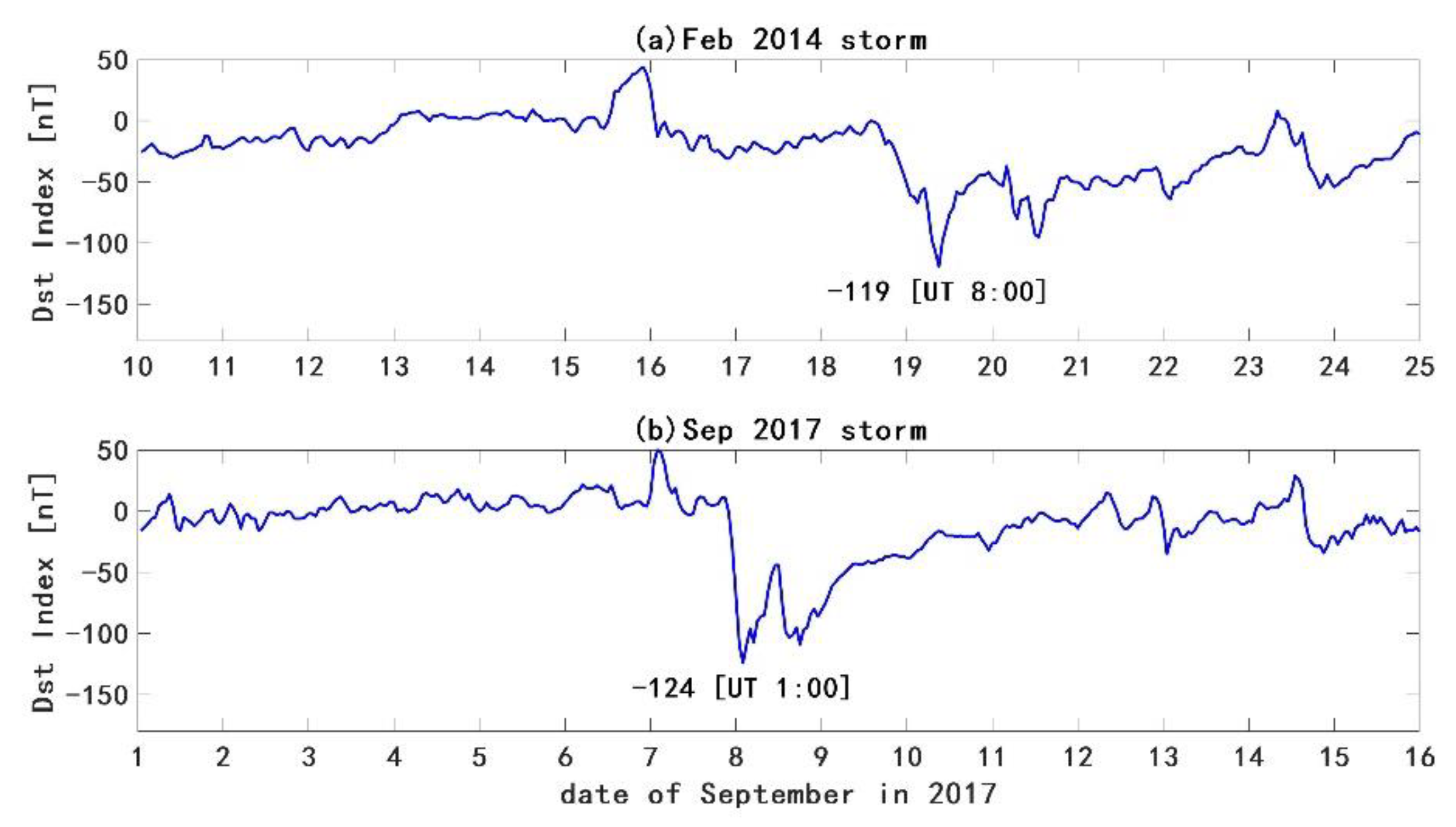
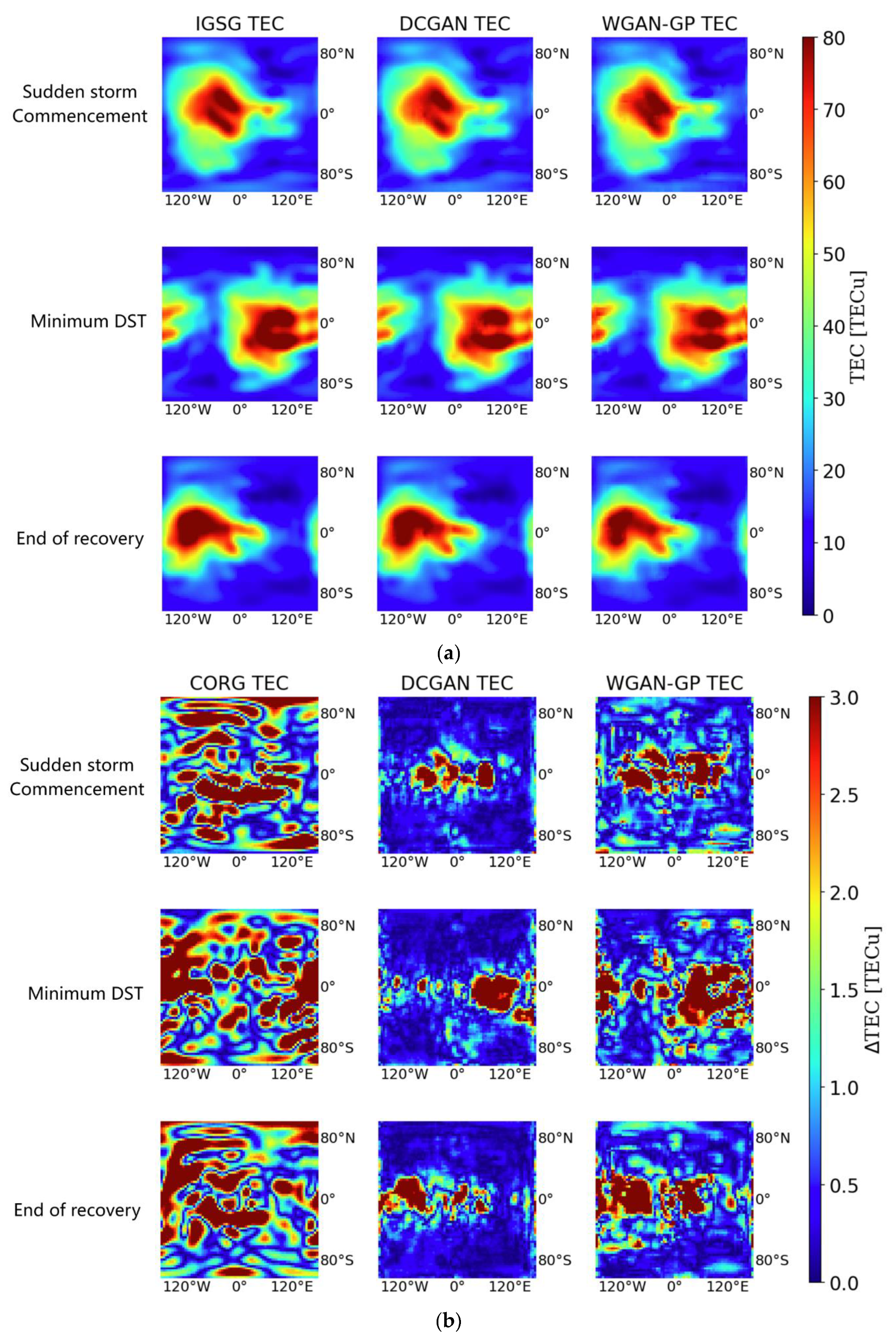
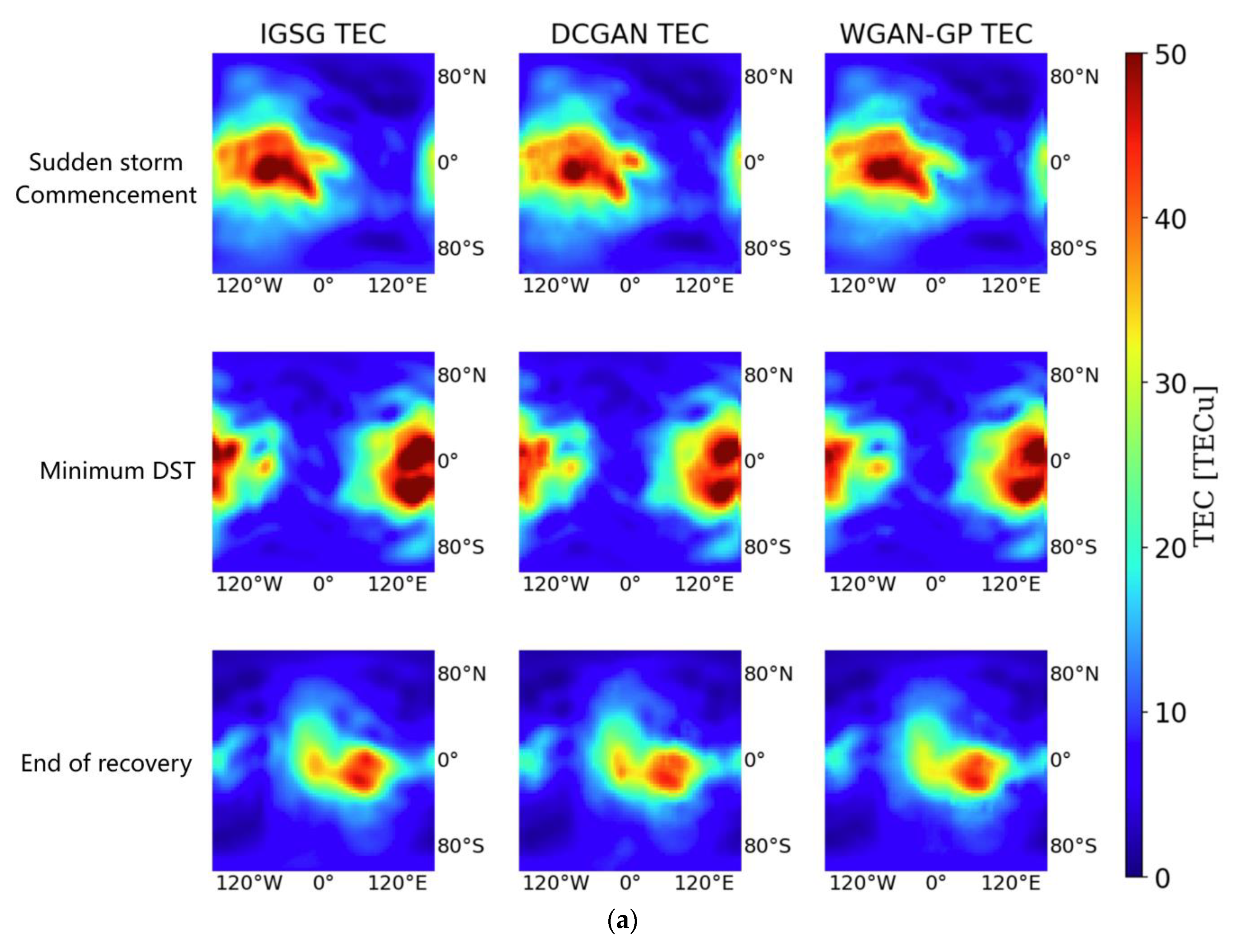
The selected geomagnetic storm in 2014 started at 15:00 UT on February 18 and reached a minimum Dst value of −119 nT at 8:00 UT on 19 February; then, the recovery phase ended at 17:00 UT on 19 February. This strong geomagnetic storm in the solar maximum has not been extensively studied before. Figure 7a shows the Dst disturbances during the storm. The global TECs estimated by the DCGAN and WGAN-GP during the geomagnetic storms were captured and demonstrated at three points: the sudden storm commencement (SSC) at 15:00 UT, 18 February, the time for the minimum Dst point (MDP) at 8:00 UT, 19 February, and the end of the recovery phase (EOR) on 17:00 UT, 19 February.

Figure 7. Temporal variation in Dst indices during the two geomagnetic storms.

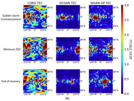
In Figure 7b, the selected geomagnetic storm in 2017 started at 20:00 UT on 7 September and reached a minimum Dst value of −124 nT at 1:00 UT on September 8; then, the recovery phase ended at 3:00 UT on 10 September. This event lasted for a long time and was attributed to CME. Figure 7b shows the Dst disturbances during the storm. The global TECs estimated by the DCGAN and WGAN-GP during the geomagnetic storms were captured and demonstrated at three points: the sudden storm commencement (SSC) at 20:00 UT, 7 September, the time for the minimum Dst point (MDP) at 1:00 UT, 8 September, and the end of the recovery phase (EOR) at 3:00 UT, 10 September.

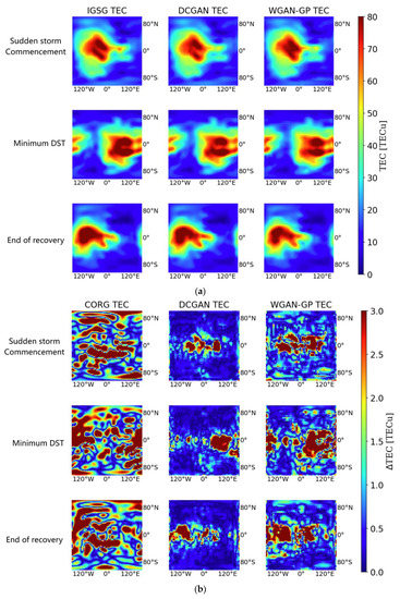
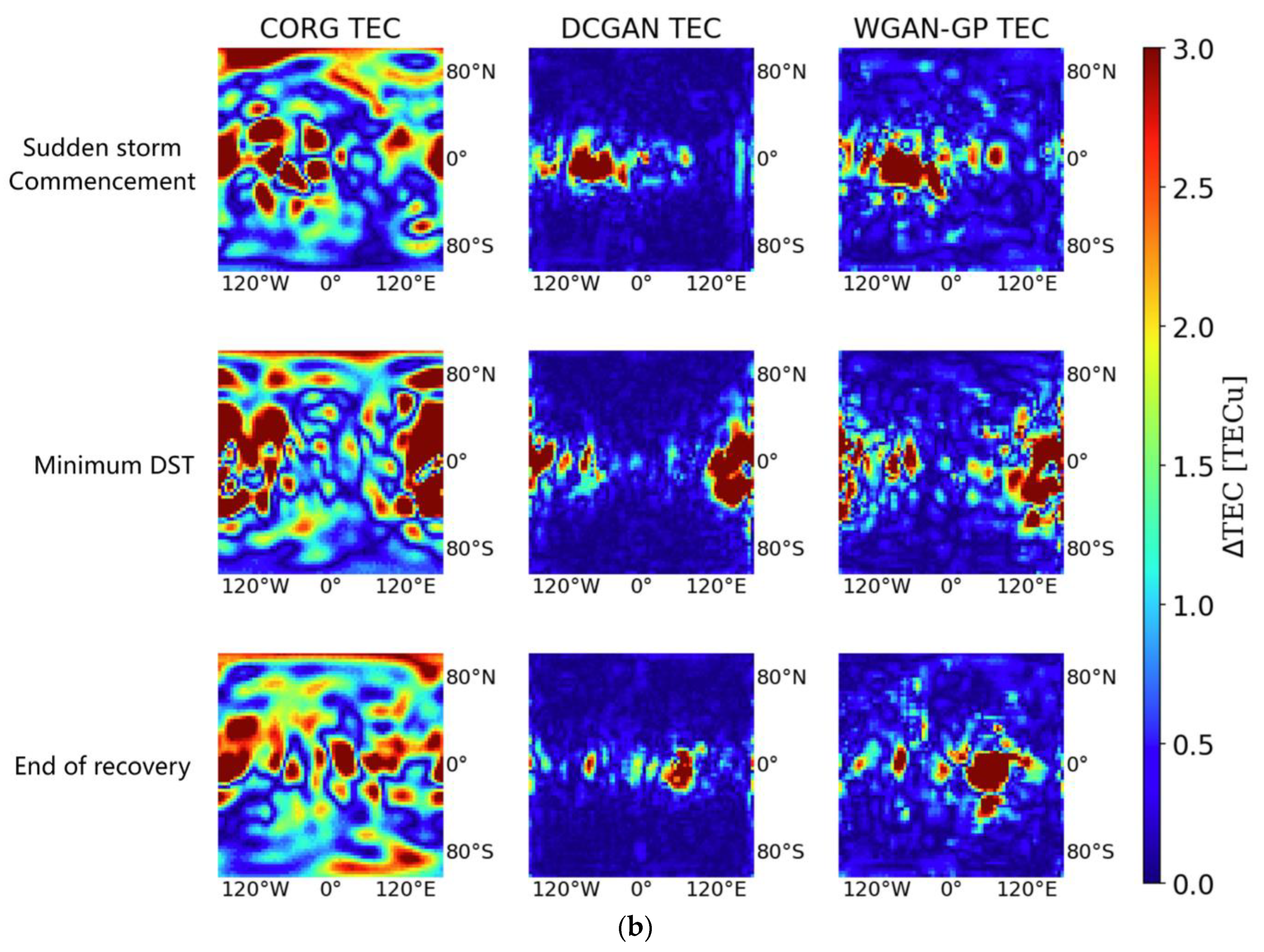
The spatial TEC completion results for the geomagnetic storm on 18 February 2014 are presented in Figure 8. Figure 8a shows that both the DCGAN and WGAN-GP captured the spatiotemporal TEC features during the geomagnetic storms. Figure 8b shows the performance in terms of the RMSE and MAE. It is noticed that the DCGAN achieved the best performance in the spatial RMSE and MAE during the geomagnetic storm. Table 4 shows the performance details for these three methods, and DCGAN even had a 22.65% lead compared to the WGAN-GP in the RMSEs below 1 TECu, and an 8.83% lead over the WGAN-GP in the MAEs below 1 TEC. Apparently, the geomagnetic storm greatly changed the feature of the ionospheric TEC from the aspects of both the RMSE and MAE. The details of the RMSE and MAE performance during this storm are listed in Table 4.

Figure 8. The ionospheric TEC (a) and the ionospheric TEC difference (b) for the geomagnetic storm on 18 February 2014. The sudden storm commencement, minimum DST, and end of recovery indicate three time points for the geomagnetic storm, as described above.

Table 4. RMSE and MAE performance during geomagnetic storm in February 2014.

		CORG	DCGAN	WGAN-GP
RMSE (TECu)	SSC	2.4698	1.3633	1.8226
	MDP	3.0273	1.8354	2.2437
	EOR	2.5193	1.1059	1.9258
	All	2.1243	0.7921	1.3889
	<1 TECu	10.26%	74.92%	52.27%
MAE (TECu)	SSC	1.8339	0.6314	1.0846
	MDP	2.2314	0.7251	1.3760
	EOR	1.9125	0.5993	1.1504
	All	0.4521	0.8817	0.7934
	<1 TECu	45.21%	88.17%	79.34%

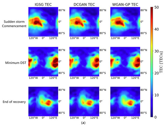
The spatial TEC completion results for the geomagnetic storm on 7 September 2017, are presented in Figure 9. Figure 9a presents the global feature of the ionosphere TEC during the geomagnetic period. Figure 9b shows the performances in terms of the RMSE and MAE. In this geomagnetic storm, the DCGAN achieved the best performance with the fewest difference in accordance with the IGS final product., but the performance difference between the DCGAN and WGAN-GP in the RMSE and MAE was narrowed. Based on the variations in the RMSE and MAE during the whole geomagnetic storm, it is indicated that the feature of the ionospheric TEC was greatly changed, as shown in Table 5.

Figure 9. The ionospheric TEC (a) and the ionospheric TEC difference (b) for the geomagnetic storm on 7 September 2017. The sudden storm commencement, minimum DST, and end of recovery indicate three time points for the geomagnetic storm, as described above.

Table 5. RMSE and MAE performance during geomagnetic storm in September 2017.

		CORG	DCGAN	WGAN-GP
RMSE (TECu)	SSC	1.4996	0.8421	1.2798
	MDP	2.6368	1.3282	1.4814
	EOR	1.4487	0.5486	1.1164
	All	1.3207	0.4874	0.7836
	<1 TECu	41.37%	83.78%	73.12%
MAE (TECu)	SSC	1.3179	0.3602	0.6413
	MDP	1.7773	0.5580	0.7773
	EOR	1.4180	0.2543	0.5608
	All	0.4018	0.0595	0.4480
	<1 TECu	59.29%	92.76%	91.90%

3.3. Diurnal Accuracy for TEC Spatial Estimation

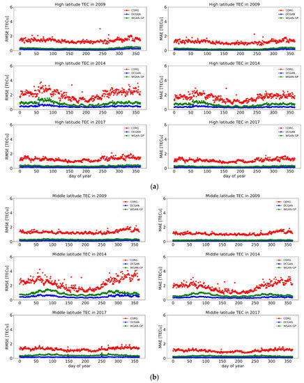
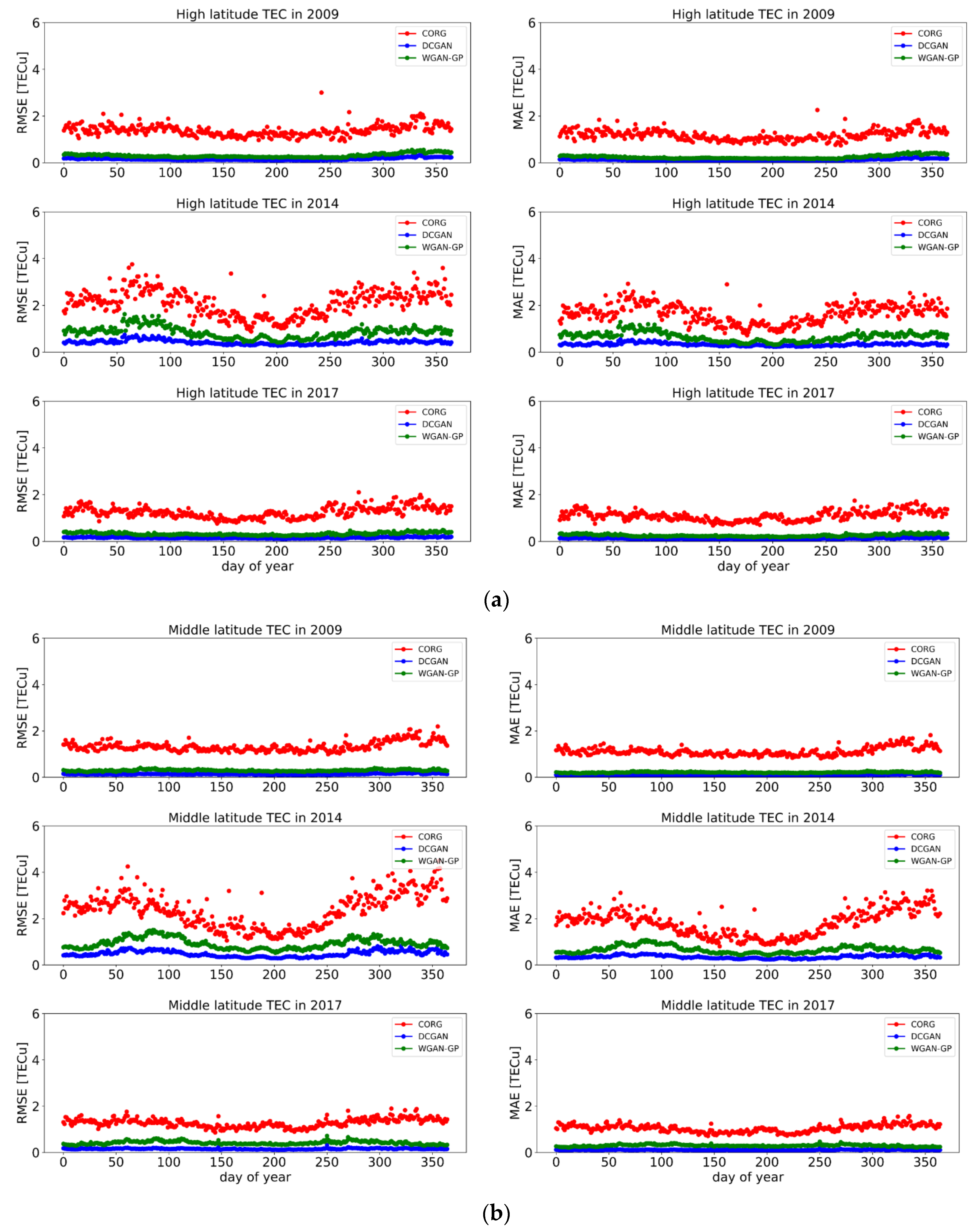
The diurnal accuracies of the TEC spatial estimations in 2009, 2014, and 2017 were analyzed, and the RMSE and MAE were computed with the daily differences between the CORG, DCGAN, and WGAN-GP and the IGS final product. All the spatial grid points were considered for the RMSE and MAE statistics, as demonstrated in Figure 10. Figure 10a shows the RMSE and MAE for the three methods in high latitudes, which cover the regions of 87.5°S–60°S and 60°N–87.5°N. It is noticed that all the RMSEs and MAEs of the DCGAN and WGAN were below 2 TECu for the daily statistics, and the performance of the DCGAN ranked the best of the three methods. The daily RMSEs and MAEs for the CORG had more fluctuations in 2014, the solar maximum year, with maximum RMSEs of 3.0041 TECu in 2009 and 3.7559 TECu in 2014. The daily RMSE also revealed seasonal TEC fluctuation, with relatively large values in spring and autumn and the lowest values in summer. This shows that the CORG had the largest daily RMSEs for all test years. The daily RMSEs were closely related to the solar activity, for instance, the daily RMSEs for the CORG, DCGAN and WGAN-GP were larger in 2014 than those in 2009 and 2017. The maximum RMSEs were 3.7559 TECu, 0.7379 TECu, and 1.6223 TECu for the CORG, DCGAN, and WGAN-GP in March 2014, when the solar maximum phase appeared in solar cycle 24.

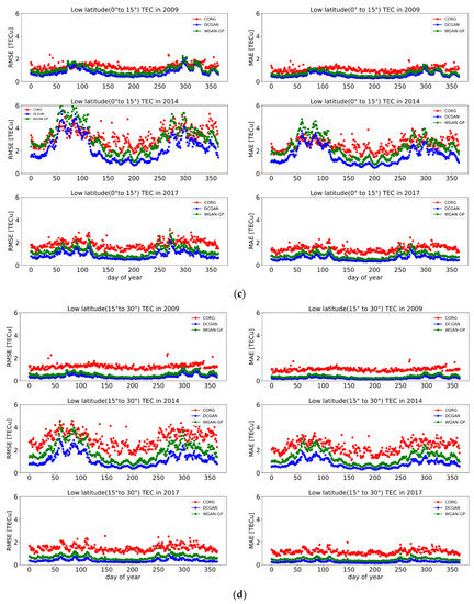
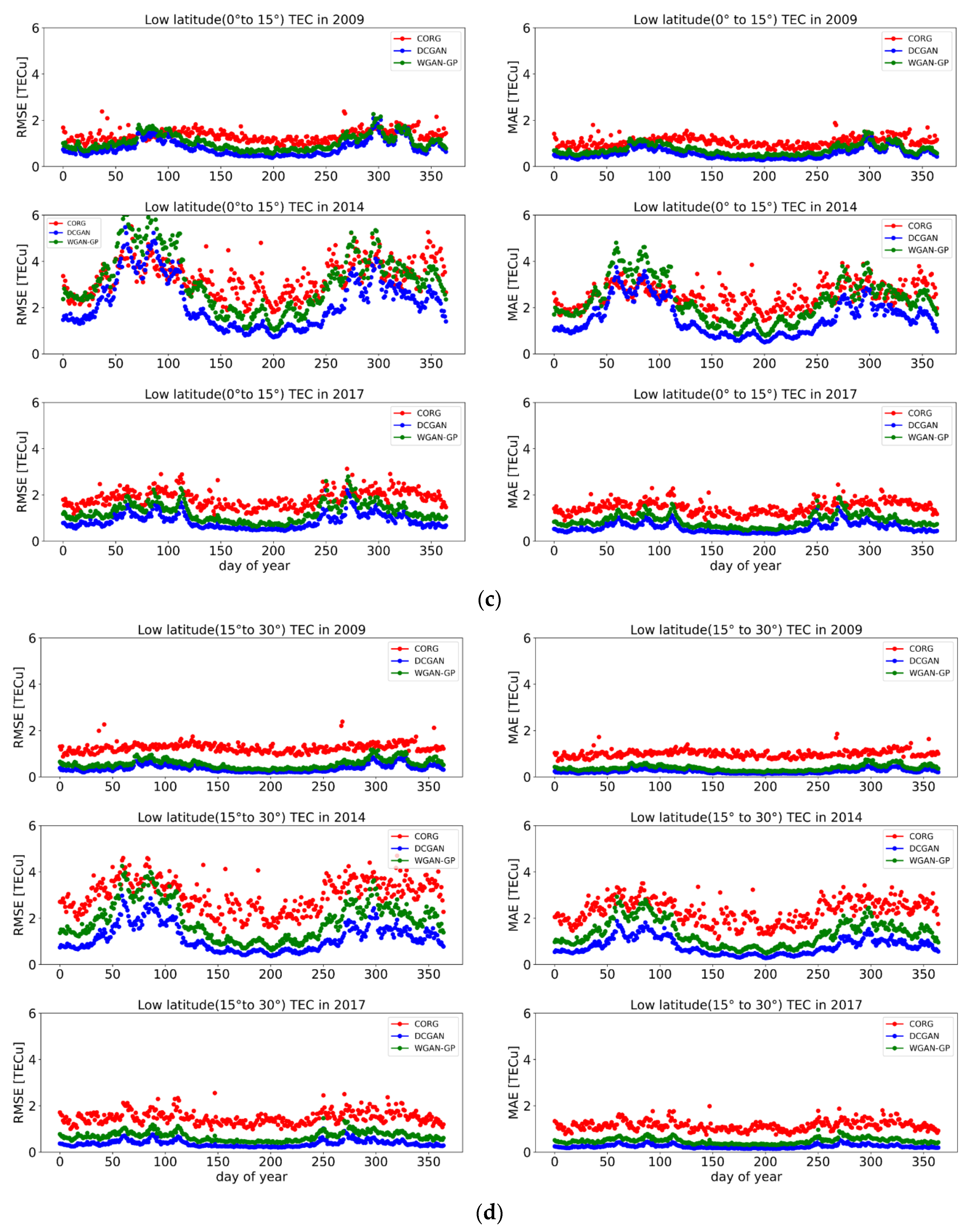
Figure 10. The daily RMSE and MAE in high latitude (87.5°S–60°S, 60°N–87.5°N), midlatitude (60°S–30°S, 30°N–60°N), and low latitude (30°S–30°N) for CORG (red dots), DCGAN (blue dots), and WGAN-GP (green dots) in 2009, 2014, and 2017.

Similar features are noticed in Figure 10b for 2009 and 2017, showing that the RMSEs and MAEs in the midlatitudes were all below 2 TECu for the CORG, DCGAN, and WGAN-GP. Meanwhile, the RMSEs and MAEs for the CORG in 2014 were larger and had stronger fluctuation than those in the high latitudes, with maximum RMSE and MAE values of 4.4938 TECu and 3.2094 TECu, respectively. The results in the low latitudes were divided into two parts: one is in the absolute latitudes of 0°–15°, and the other is in the absolute latitudes of 15°–30° in both the north and south hemispheres, as shown in Figure 10c,d. This indicates that the RMSEs and MAEs of the low latitudes in 2009 and 2017 were all less than 3 TECu, and the maximum RMSE and MAE values for the DCGAN were 0.9432 TECu and 0.5337 TECu in 2009, and 1.0233 TECu and 0.5950 TECu in 2017 for the absolute latitudes in 15°–30°. The RMSEs and MAEs in 2014 demonstrated very strong fluctuations in the daily statistics, and the maximum RMSEs were 4.6971 TECu, 2.9718 TECu, and 4.2541 TECu for the CORG, DCGAN, and WGAN-GP, respectively, and the maximum MAEs were 3.5072 TECu, 1.8822 TECu, and 2.9270 TECu. This reveals that the daily statistics for the DCGAN achieved the best approximation to the IGS final product compared to the CORG and WGAN-GP. Similar features can be seen for the absolute latitudes of 0°–15°, with larger maximum RMSEs and MAEs for all three methods. For the absolute latitudes of 0°–15°, the maximum RMSEs of the DCGAN were 2.0792 TECu in 2009, 5.4733 TECu in 2014, and 2.2079 TECu in 2017. The average RMSEs of the DCGAN were 0.8174 TECu in 2009, 2.2204 TECu in 2014, and 0.8738 TECu in 2017. Similar features can be seen for the MAEs in the same region.

4. Discussion

The spatial TEC estimation performance is related to solar and geomagnetic activities as well as the nature of the ionospheric variation in latitude and longitude.

For both the DCGAN and WGAN-GP, the networks of the generator to extract the statistical features of the original data were identical, and the network of the discriminator was different due to the framework of the WGAN-GP. It is shown that the WGAN-GP had a larger RMSE and MAE for the TEC regional estimation compared to the DCGAN for all the testing years.

The spatial TEC estimation clearly agrees with the solar activity trend, with better accuracy in the solar descending phase than in the solar ascending phase, which is consistent with the previous study regarding the impact of solar activity on the performance of the GIM products [23]. The RMSE difference had a maximum of 1.2548 TECu between the results of 2009 and 2014 for the DCGAN, and a maximum of 1.8066 TECu between the results of 2009 and 2014 for the WGAN-GP. Similarly, the MAE differences had a maximum of 2.6437 TECu between the results of 2009 and 2014 for the DCGAN and a maximum of 2.9157 TECu between the results of 2009 and 2014 for the WGAN-GP.

Two strong geomagnetic storms were selected for this study. The RMSEs during the geomagnetic storm on 18 February 2014 worsened by 0.8058 TECu (CORG), 0.6159 TECu (DCGAN), and 0.4909 TECu (WGAN-GP) compared to the daily statistics. The MAEs during the geomagnetic storm on 18 February 2014 worsened by 1.1010 TECu (CORG), 0.3299 TECu (DCGAN), and 0.8170 TECu (WGAN-GP) compared to the daily statistics. The RMSEs during the geomagnetic storm on 7 September 2017 worsened by 1.7749 TECu (CORG), 1.0578 TECu (DCGAN), and 0.9671 TECu (WGAN-GP) compared to the daily statistics. The MAEs during the geomagnetic storm on February 18, 2014 worsened by 0.9154 TECu (CORG), 0.4323 TECu (DCGAN), and 0.5634 TECu (WGAN-GP) compared to the daily statistics.

The results are comparable to previous work using a DCGAN-PB and SNP-GAN for both high and low solar activity years [18,19]. In a previous study, two moderate geomagnetic storms were selected (17 March 2013 and 3 February 2016), and the maximum RMSEs were 7.4214 for the IGS GIM and 4.2054 for the SNP-GAN. In this work, two strong geomagnetic storms were studied (18 February 2014, and 7 September 2017), and the maximum RMSEs were 0.83 and 1.05 for the DCGAN and WGAN-GP, respectively.

Generally, the spatial TEC estimation accuracy is closely related to the nature of ionospheric variations in latitude and longitude. The RMSE and MAE are relatively small in high-latitude regions than in middle- and low-latitude regions. The most difficult regions for TEC estimation are the low-latitude regions, especially the equatorial ionization anomaly regions. For these cases, it is worth attempting to improve the estimation performance in the EIA region using a spatial adaptive GAN framework, in which the generator and discriminator networks can be adjusted with ionospheric latitudinal variation features.

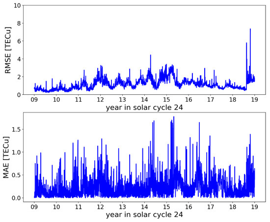
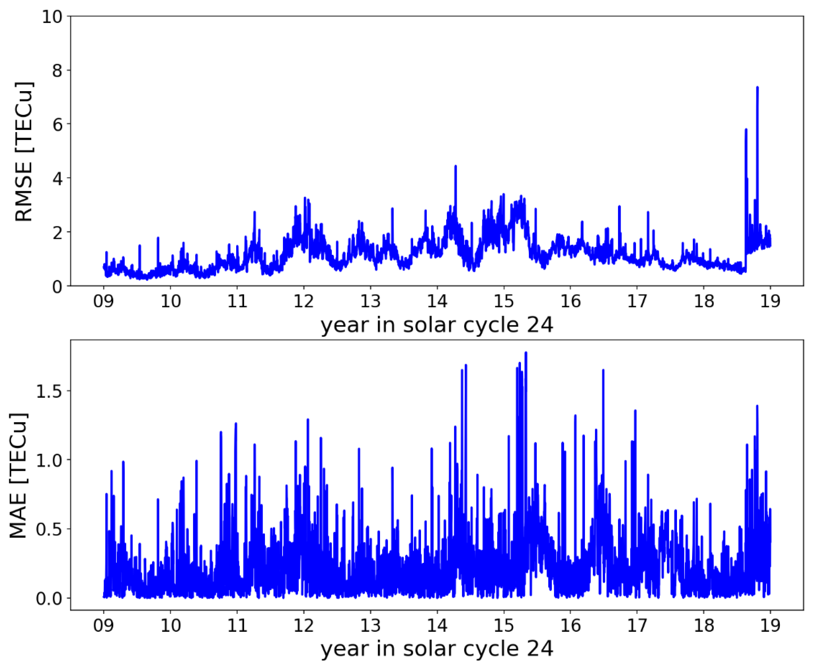
For both point and regional TEC estimation, it is shown that the GAN-based framework outperformed the IGS rapid product. The IGS rapid TEC prediction started in 2004, and its performance remained stable for years, as Figure 11 shows. Meanwhile, compared to the GAN-based framework, the IGS rapid prediction accuracy still requires more improvement. This is a way to use a deep learning framework to produce rapid products in the near future. Moreover, with flexible generator and discriminator networks, the GAN-based framework has much potential for spatial TEC estimation improvement and high-resolution TEC description.

Figure 11. The daily RMSE and MAE for CORG in solar cycle 24.

5. Conclusions

In this work, two types of GAN-based frameworks were constructed and validated for spatial point and regional TEC estimation. The IGS GIM final product from 2000 to 2017 was used for the training and testing databases, and the data from 2009, 2014, and 2017 were used for testing when they were excluded from the training databases. The experiments revealed that both the DCGAN and WGAN-GP can achieve acceptable spatial TEC estimation accuracy and demonstrated great advantages over the IGS rapid products in point and regional TEC estimation. The solar activity and geomagnetic disturbances were considered, showing that the TEC estimation accuracy of the GAN-based framework was also influenced by different solar phases, and the global average RMSEs in the solar maximum were 0.7695 TECu (DCGAN) and 1.3317 TECu (WGAN-GP), which are greater than those in the solar minimum. For the DCGAN, the average TEC RMSE and MAE were 0.6159 TECu and 0.3299 TECu higher during the geomagnetic storm on 18 February 2014, respectively, than those under normal conditions, and 1.0578 TECu and 0.4323 TECu higher during the geomagnetic storm on 7 September 2017, respectively, than those under normal conditions. For the WGAN-GP, the average TEC RMSE and MAE were 0.4909 TECu and 0.8170 TECu higher during the geomagnetic storm on 18 February 2014, respectively, than those under normal conditions, and 0.9671 TECu and 0.5634 TECu higher, respectively, than those under normal conditions during the geomagnetic storm on 7 September 2017.

The RMSEs and MAEs for different latitudes were also investigated; this reveals that the DCGAN achieved the best performance for all latitudes, but the RMSE and MAE increased from high latitude to low latitude. Specifically, the average RMSEs for the DCGAN in the equatorial ionization anomaly region (15°S–15°N) were 5.27 times, 5.29 times, and 5.82 times larger than those in high latitudes in 2009, 2014, and 2017, respectively. In the same condition, the average MAEs were 4.69 times, 4.74 times, and 5.16 times larger in the equatorial ionization anomaly region than those in high latitudes in 2009, 2014, and 2017.

The GAN-based framework can extract the detailed features of the spatial TEC responses to geomagnetic storms. Further investigation can be conducted to improve the generator and discriminator architecture of the GAN-based framework for better and higher spatial descriptions of TEC morphology.

References

- Klobuchar, J.A. Ionospheric time-delay algorithms for single-frequency gps users. IEEE Trans. Aerosp. Electron. Syst. 1987, AES-23, 325–331. [Google Scholar] [CrossRef] [Scilit]
- Prieto-Cerdeira, R.; ROrús-Pérez Breeuwer, E.; Lucas-Rodriguez, R.; Falcone, M. Performance of the Galileo Single-frequency Ionospheric Correction during In-Orbit Validation. GPS World 2014, 25, 53–58. [Google Scholar]
- Yuan, Y.; Wang, N.; Li, Z.; Huo, X. The beidou global broadcast ionospheric delay correction model (BDGIM) and its preliminary performance evaluation results. Navigation 2019, 66, 55–69. [Google Scholar] [CrossRef] [Scilit]
- Hernández-Pajares, M.; Juan, J.M.; Sanz, J.; Orus, R.; Garcia-Rigo, A.; Feltens, J.; Komjathy, A.; Schaer, S.C.; Krankowski, A. The IGS VTEC Maps: A Reliable Source of Ionospheric Information Since 1998. J. Geod. 2009, 83, 263–275. [Google Scholar] [CrossRef] [Scilit]
- Roma-Dollase, D.; Hernández-Pajares, M.; Krankowski, A.; Kotulak, K.; Ghoddousi-Fard, R.; Yuan, Y.; Li, Z.; Zhang, H.; Shi, C.; Wang, C.; et al. Consistency of seven different GNSS global ionospheric mapping techniques during one solar cycle. J. Geod. 2018, 92, 691–706. [Google Scholar] [CrossRef] [Scilit]
- Bilitza, D.; Altadill, D.; Truhlik, V.; Shubin, V.; Galkin, I.; Reinishch, B.; Huang, X. International Reference Ionosphere 2016: From ionospheric climate to real-time weather predictions. Space Weather 2017, 15, 418–429. [Google Scholar] [CrossRef] [Scilit]
- Nava, B.; Coïsson, P.; Radicella, S.M. A new version of the Nequick ionosphere electron density model. J. Atmos. Sol.-Terr. Phys. 2008, 70, 1856–1862. [Google Scholar] [CrossRef] [Scilit]
- Han, Y.; Wang, L.; Fu, W.; Zhou, H.; Li, T.; Chen, R. Machine Learning-Based Short-Term GPS TEC Forecasting During High Solar Activity and Magnetic Storm Periods. IEEE J. Sel. Top. Appl. Earth Obs. Remote Sens. 2022, 15, 115–126. [Google Scholar] [CrossRef] [Scilit]
- Liu, L.; Zou, S.; Yao, Y.; Wang, Z. Forecasting global ionospheric TEC using deep learning approach. Space Weather 2020, 18, e2020SW002501. [Google Scholar] [CrossRef] [Scilit]
- Zhukov, A.; Sidorov, D.; Mylnikova, A.; Yasyukevich, Y. Machine learning methodology for ionosphere total electron content nowcasting. Int. J. Artif. Intell. 2018, 16, 144–157. [Google Scholar]
- Ruwali, A.; Kumar, A.; Prakash, K.B.; Gampala, S.; Ratnam, V. Implementation of hybrid deep learning model (LSTM-CNN) for ionospheric TEC forecasting using GPS data. IEEE Geosci. Remote Sens. Lett. 2020, 18, 1004–1008. [Google Scholar] [CrossRef] [Scilit]
- Kaselimi, M.; Voulodimos, A.; Doulamis, N.; Doulamis, A.; Delikaraoglou, D. Deep Recurrent Neural Networks for Ionospheric Variations Estimation Using GNSS Measurements. IEEE Trans. Geosci. Remote Sens. 2022, 60, 5800715. [Google Scholar] [CrossRef] [Scilit]
- Bi, C.; Ren, P.; Yin, T.; Zhang, Y.; Li, B.; Xiang, Z. An Informer Architecture-Based Ionospheric foF2 [1312] Model in the Middle Latitude Region. IEEE Geosci. Remote Sens. Lett. 2022, 19, 1005305. [Google Scholar] [CrossRef] [Scilit]
- Srivani, I.; Prasad, S.V.; Ratnam, D. A Deep Learning-Based Approach to Forecast Ionospheric Delays for GPS Signals. IEEE Geosci. Remote Sens. Lett. 2019, 16, 1180–1184. [Google Scholar] [CrossRef] [Scilit]
- Chen, Z.; Jin, M.; Deng, Y.; Wang, J.-S.; Huang, H.; Deng, X.; Huang, C.-M. Improvement of a deep learning algorithm for total electron content maps: Image completion. J. Geophys. Res. Space Phys. 2019, 124, 790–800. [Google Scholar] [CrossRef] [Scilit]
- Chen, J.; Fang, H.; Liu, Z. The application of a deep convolutional generative adversarial network on completing global TEC maps. J. Geophys. Res. Space Phys. 2021, 126, e2020JA028418. [Google Scholar] [CrossRef] [Scilit]
- Ji, E.; Moon, Y.; Park, E. Improvement of IRI global TEC maps by deep learning based on conditional generative adversarial networks. Space Weather 2020, 18, e2019SW002411. [Google Scholar] [CrossRef] [Scilit]
- Pan, Y.; Jin, M.; Zhang, S.; Deng, Y. TEC map completion using DCGAN and Poisson blending. Space Weather 2020, 18, e2019SW002390. [Google Scholar] [CrossRef] [Scilit]
- Pan, Y.; Jin, M.; Zhang, S.; Deng, Y. TEC map completion through a deep learning model: SNP-GAN. Space Weather 2021, 19, e2021SW002810. [Google Scholar] [CrossRef] [Scilit]
- Goodfellow, I.; Pouget-Abadie, J.; Mirza, M.; Xu, B.; Warde-Farley, D.; Ozair, S.; Courville, A.; Bengio, Y. Generative Adversarial Nets. Adv. Neural Inf. Process. Syst. 2014, 27, 2672–2680. [Google Scholar]
- Radford, A.; Metz, L.; Chintala, S. Unsupervised Representation Learning with Deep Convolutional Generative Adversarial Networks. arXiv 2015, arXiv:1511.06434. [Google Scholar]
- Gulrajani, I.; Ahmed, F.; Arjovsky, M.; Dumoulin, V.; Courville, A.C. Improved Training of Wasserstein GANs. Adv. Neural Inf. Process. Syst. 2017, 30. [Google Scholar]
- Wielgosz, P.; Milanowska, B.; Krypiak, G.A.; Jarmolowski, W. Validation of GNSS derived global ionosphere maps for different solar activity levels: Case studies for years 2014 and 2018. GPS Solut. 2021, 25, 103. [Google Scholar] [CrossRef] [Scilit]
Publisher’s Note: MDPI stays neutral with regard to jurisdictional claims in published maps and institutional affiliations. |
© 2022 by the authors. Licensee MDPI, Basel, Switzerland. This article is an open access article distributed under the terms and conditions of the Creative Commons Attribution (CC BY) license (https://creativecommons.org/licenses/by/4.0/).