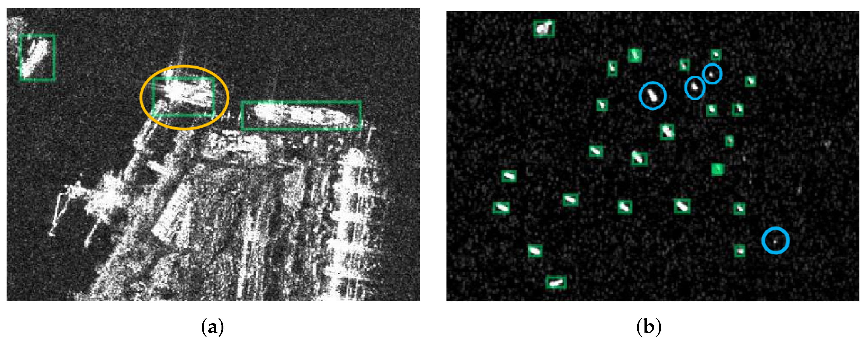
Figure 1.
Some undesired detection results under typical scenes from RetinaNet [
26]. The spring-green rectangles represent the detection results. The orange and blue circles represent the false alarms and the missing ships, respectively. (
a) False alarms in complex scenes. (
b) The missing small ships.
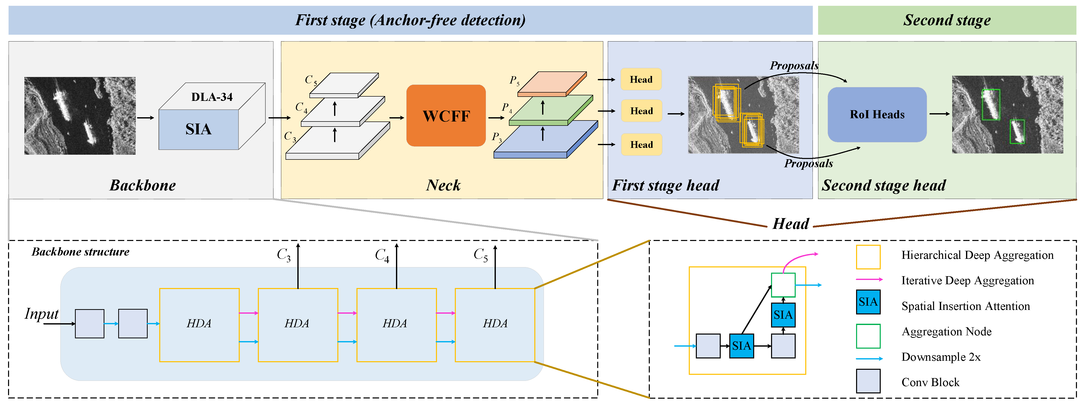
Figure 2.
The overall framework of ATSD follows the usual object detector design manner: “Backbone-Neck-Head”. The SIA module embedded in the backbone network and the WCFF module embedded in the neck block are introduced in the first stage, and the head network spans the first and second stages.
Figure 2.
The overall framework of ATSD follows the usual object detector design manner: “Backbone-Neck-Head”. The SIA module embedded in the backbone network and the WCFF module embedded in the neck block are introduced in the first stage, and the head network spans the first and second stages.
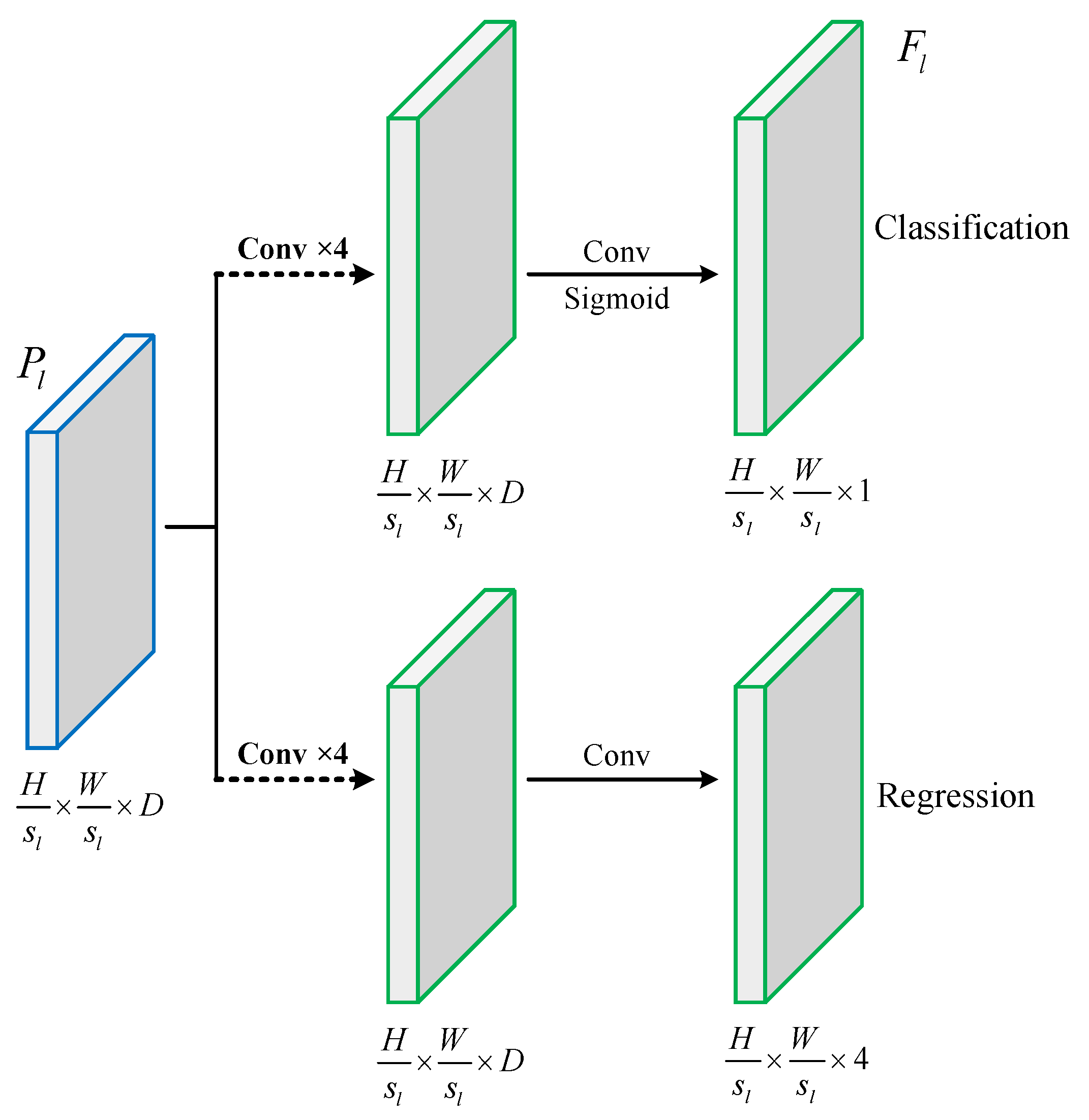
Figure 3.
Structure of the AFD head. Both branches stack five 3 × 3 convolutional layers to learn task-specific features for object classification and regression, respectively.
Figure 3.
Structure of the AFD head. Both branches stack five 3 × 3 convolutional layers to learn task-specific features for object classification and regression, respectively.
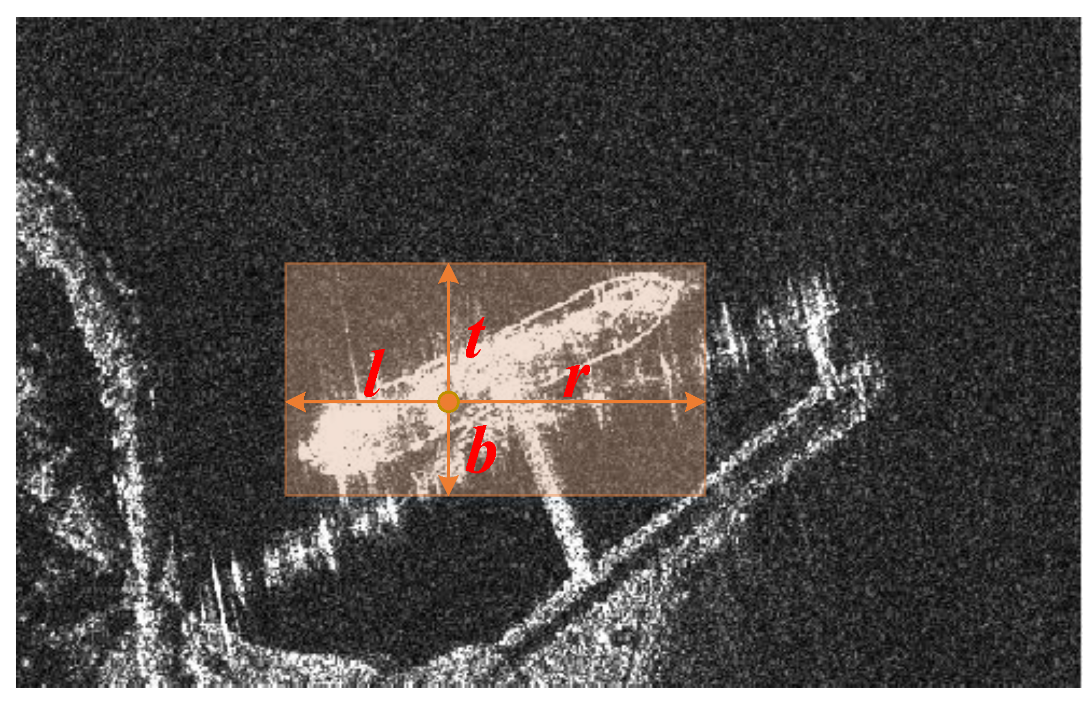
Figure 4.
A 4D vector encodes the bounding box. depicts the relative distances from the object center to the four sides of the bounding box.
Figure 4.
A 4D vector encodes the bounding box. depicts the relative distances from the object center to the four sides of the bounding box.
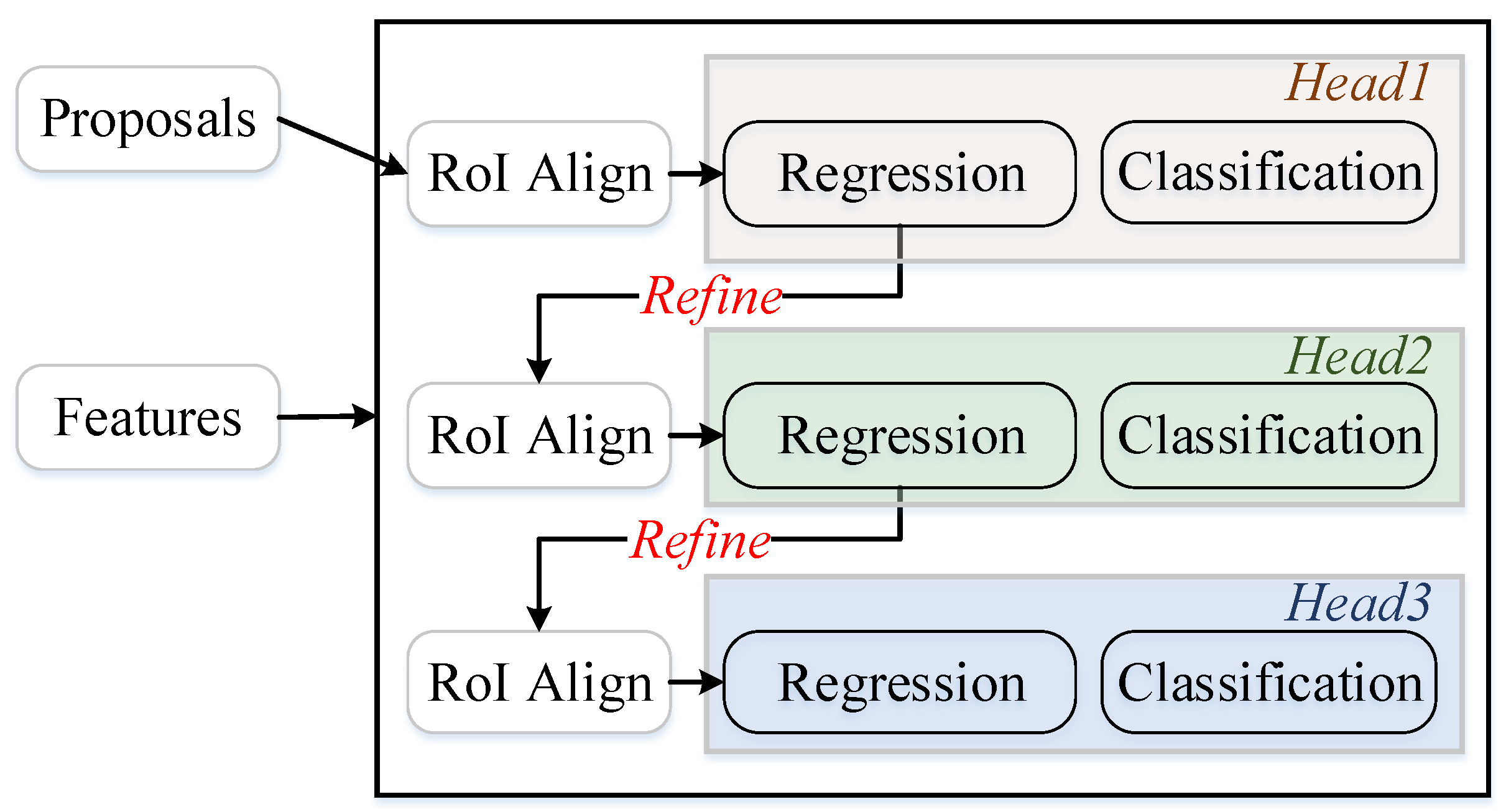
Figure 5.
Cascaded RoI heads. Three heads (Head 1, 2, 3) are trained with IoU thresholds of {0.5, 0.6, 0.7}, respectively.
Figure 5.
Cascaded RoI heads. Three heads (Head 1, 2, 3) are trained with IoU thresholds of {0.5, 0.6, 0.7}, respectively.
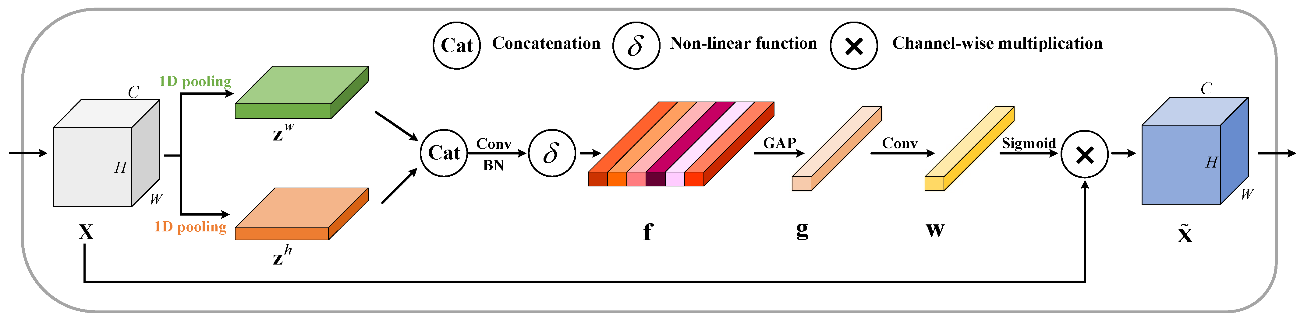
Figure 6.
The design of the spatial insertion attention (SIA) module. “Conv” and “GAP” represent a convolutional layer and a global average pooling layer. “BN” denotes batch normalization.“Sigmoid” is activation function.
Figure 6.
The design of the spatial insertion attention (SIA) module. “Conv” and “GAP” represent a convolutional layer and a global average pooling layer. “BN” denotes batch normalization.“Sigmoid” is activation function.
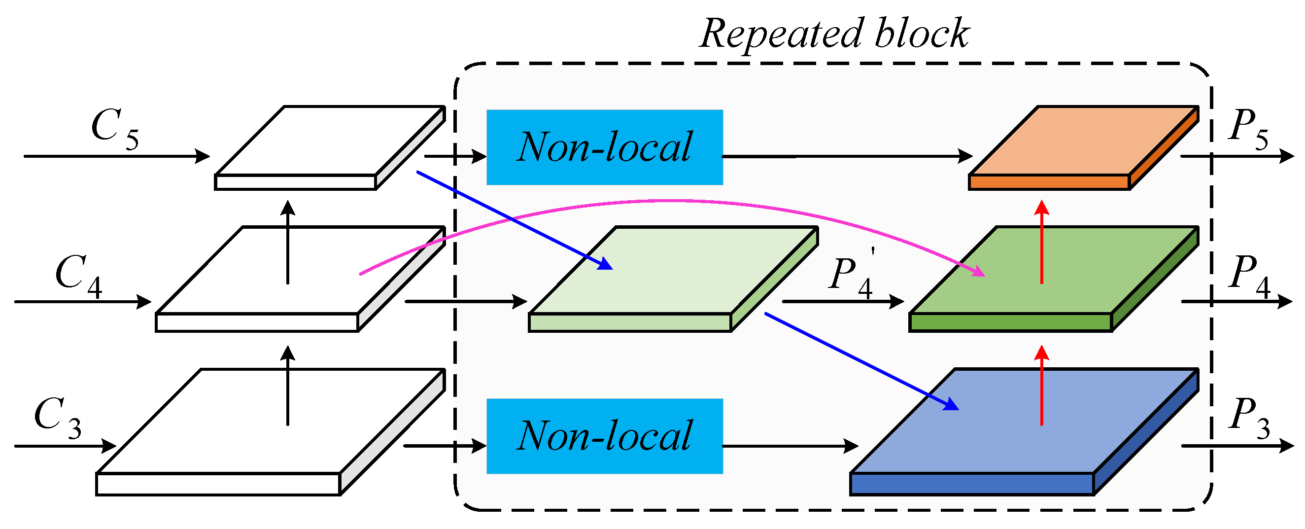
Figure 7.
The structure of WCFF module. The non-local network is embedded in the edge branch.
Figure 7.
The structure of WCFF module. The non-local network is embedded in the edge branch.
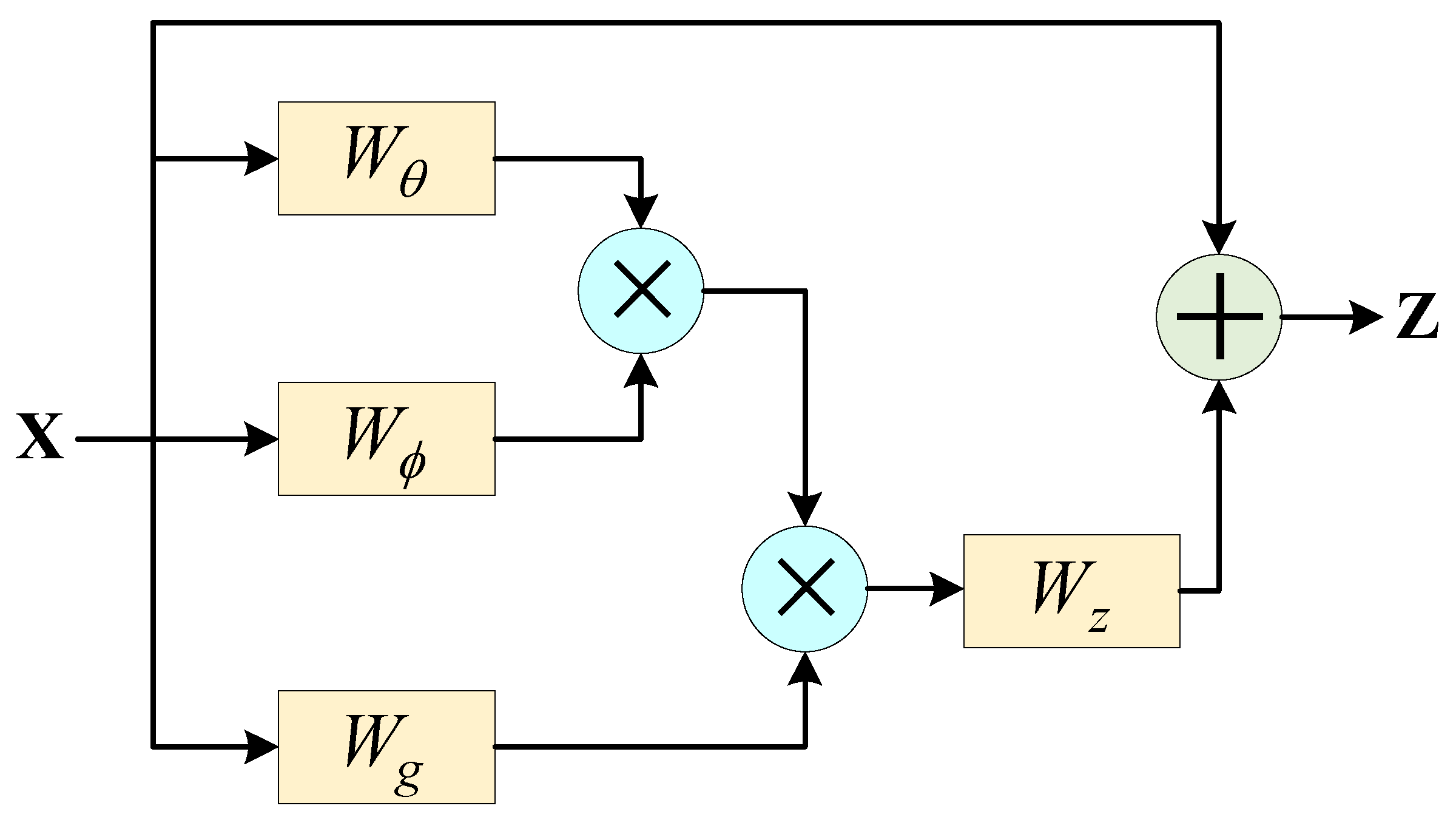
Figure 8.
A Non-local network. , , and are weight matrices to be learned.
Figure 8.
A Non-local network. , , and are weight matrices to be learned.
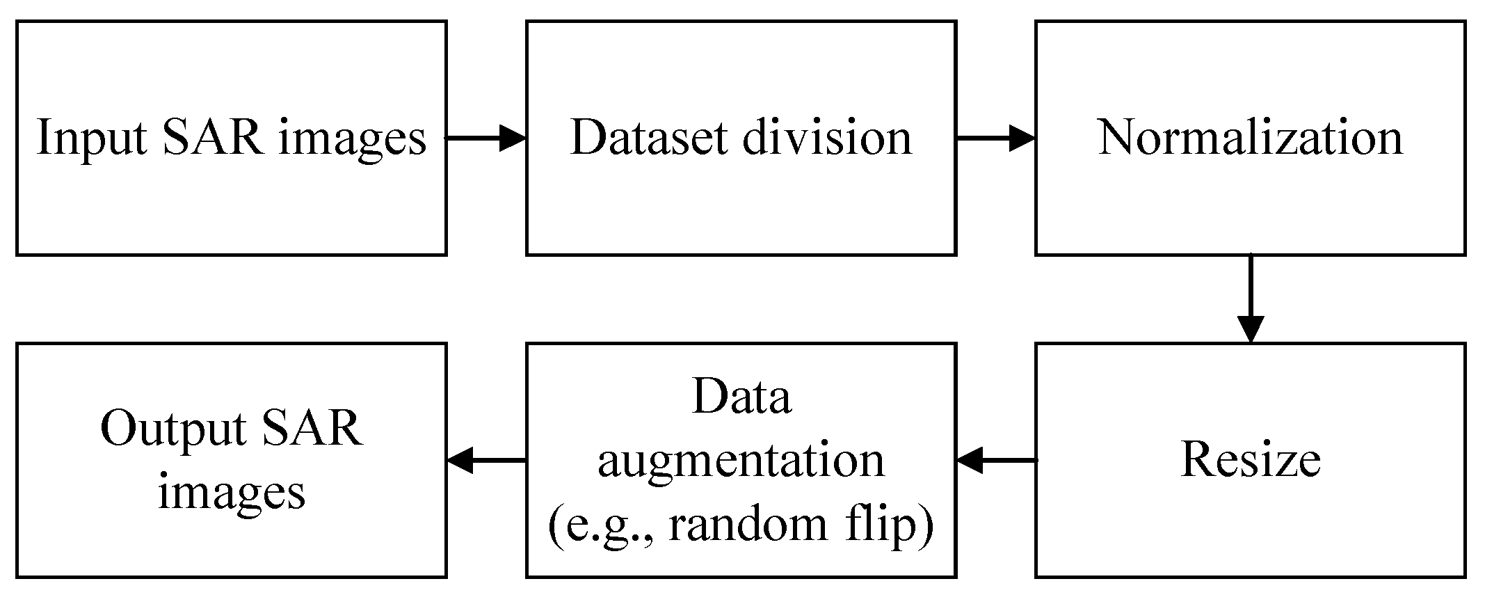
Figure 9.
A flow chart of pre-processing for SAR images.
Figure 9.
A flow chart of pre-processing for SAR images.
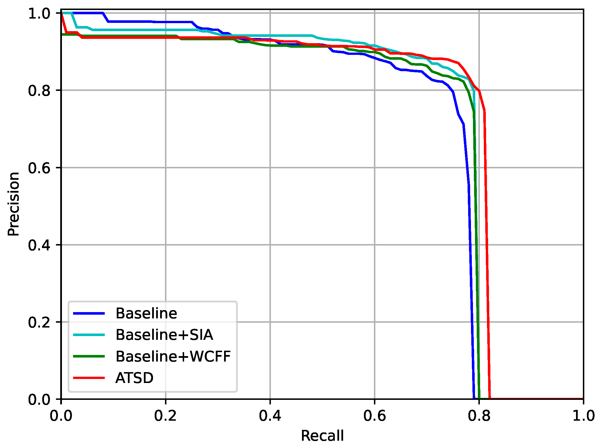
Figure 10.
PR curves of different feature enhancement modules under the IoU threshold of 0.75 on the SSDD dataset.
Figure 10.
PR curves of different feature enhancement modules under the IoU threshold of 0.75 on the SSDD dataset.
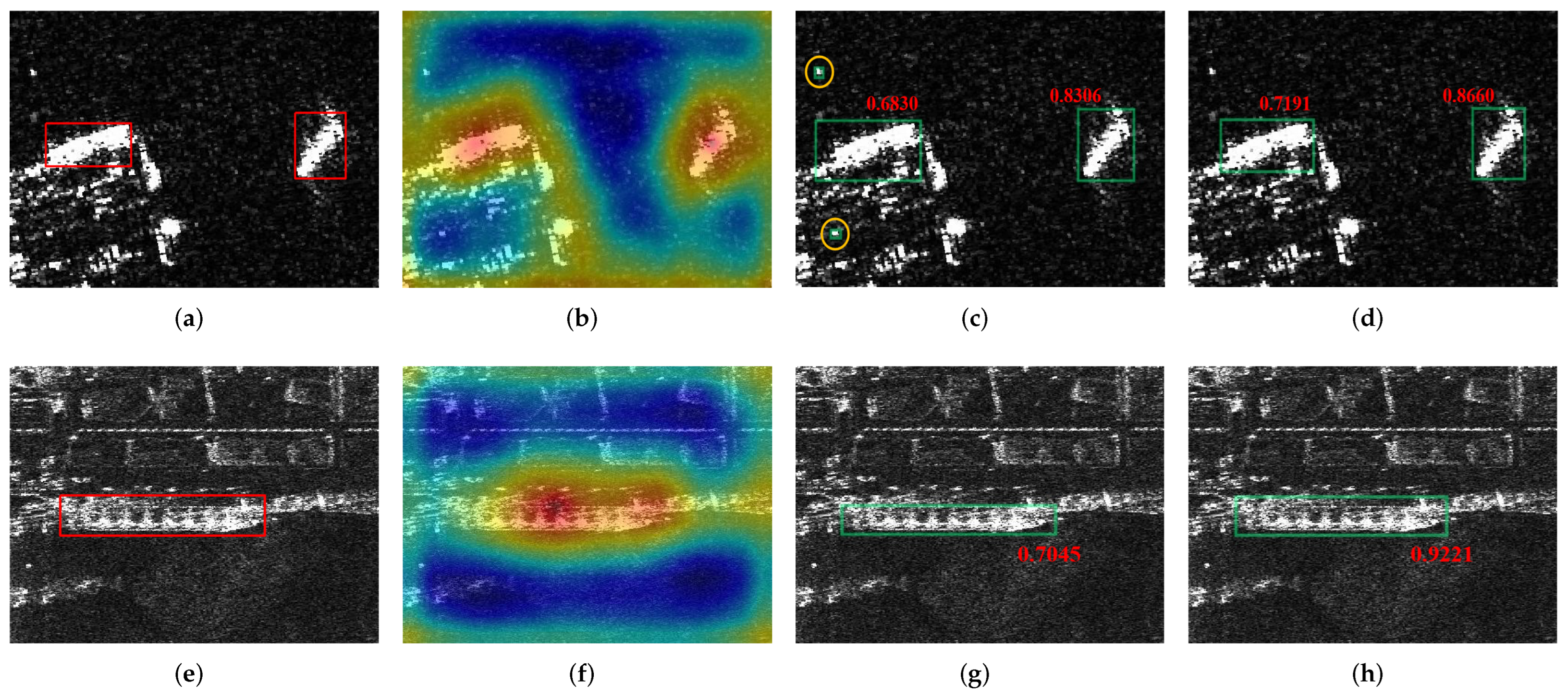
Figure 11.
Detection results of the baseline with and without SIA. The spring-green rectangles represent the detection results, and the orange circles represent the false alarms. The red number reflects the IoU between the prediction result and the corresponding ground truth. (a,e) Ground truth. (b,f) Visualization of the confidence maps with SIA. (c,g) Detection results of the baseline. (d,h) Detection results of the baseline with SIA.
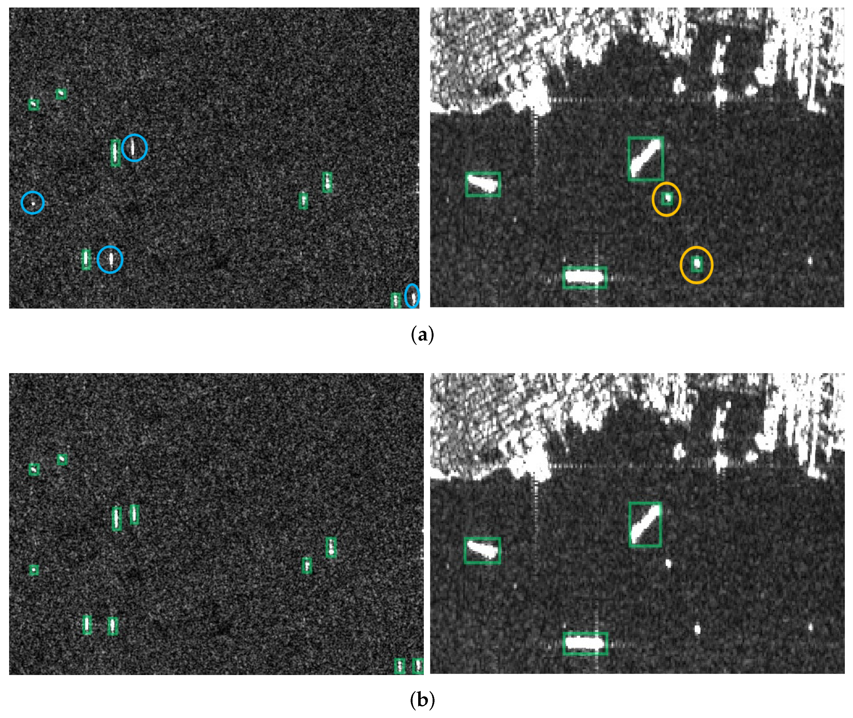
Figure 12.
Comparison results of the methods with and without WCFF. The spring-green rectangles represent the detection results. The orange and blue circles represent the false alarms and the missing ships. (a) Results of the baseline. (b) Results of the baseline with WCFF.
Figure 12.
Comparison results of the methods with and without WCFF. The spring-green rectangles represent the detection results. The orange and blue circles represent the false alarms and the missing ships. (a) Results of the baseline. (b) Results of the baseline with WCFF.
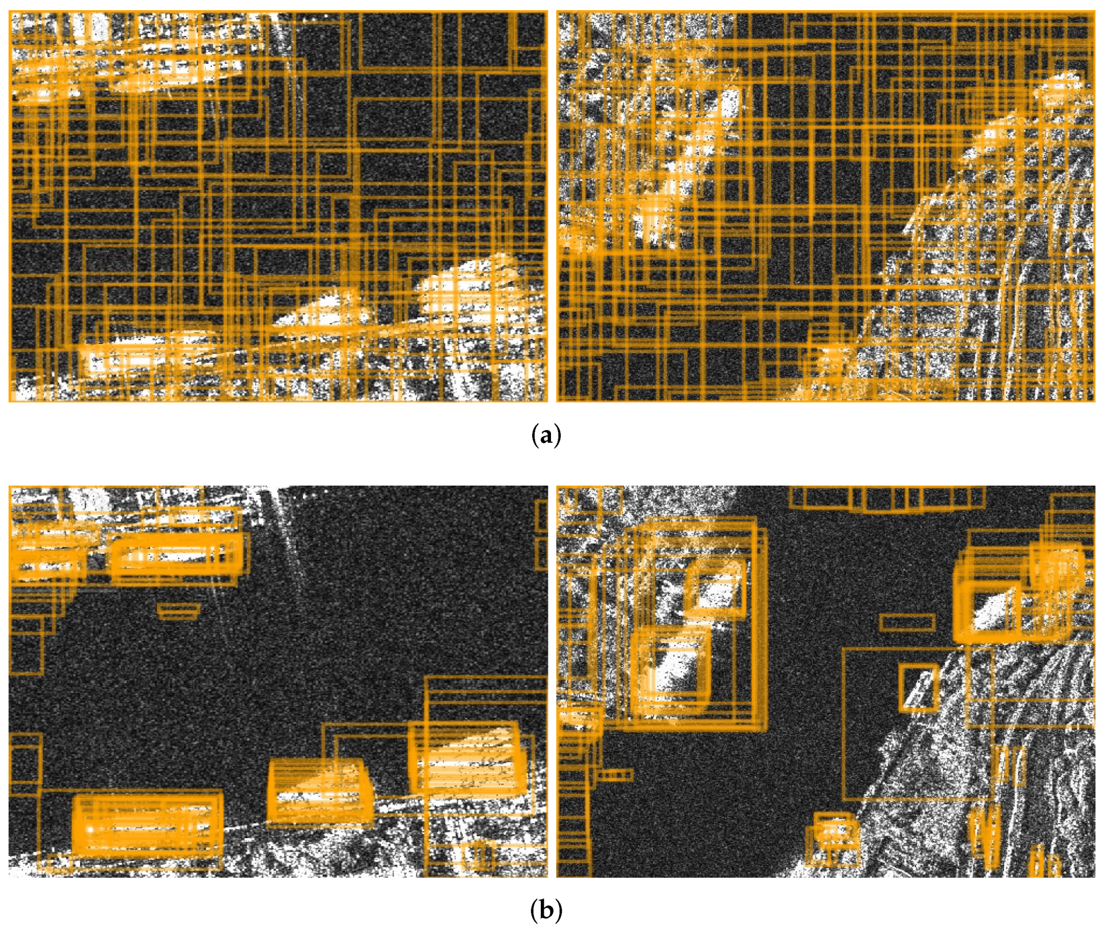
Figure 13.
Visualization of proposals generated by the conventional RPN and our AFD. (a) proposals from the RPN-based detector, for clarity, we only show proposals with its confidence score . (b) proposals from the AFD-based detector.
Figure 13.
Visualization of proposals generated by the conventional RPN and our AFD. (a) proposals from the RPN-based detector, for clarity, we only show proposals with its confidence score . (b) proposals from the AFD-based detector.
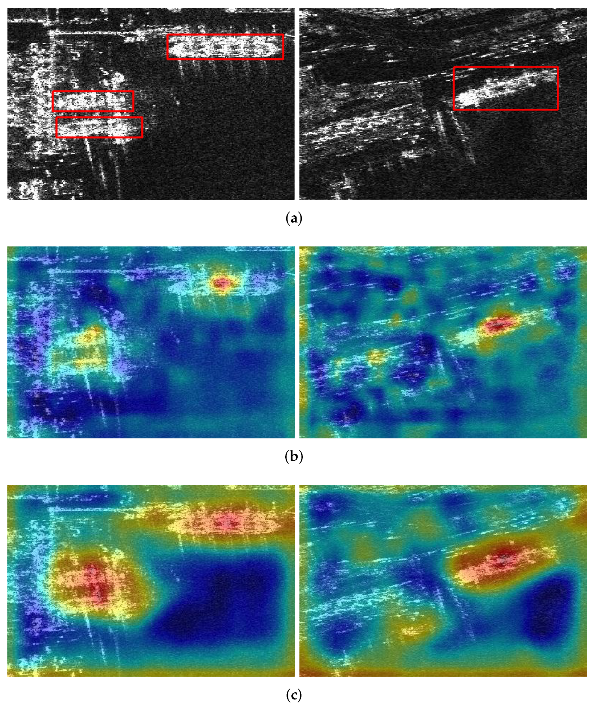
Figure 14.
Visualization of the confidence maps. (a) Ground truth. (b) Visualization of the baseline without SIA. (c) Visualization of the baseline with SIA.
Figure 14.
Visualization of the confidence maps. (a) Ground truth. (b) Visualization of the baseline without SIA. (c) Visualization of the baseline with SIA.
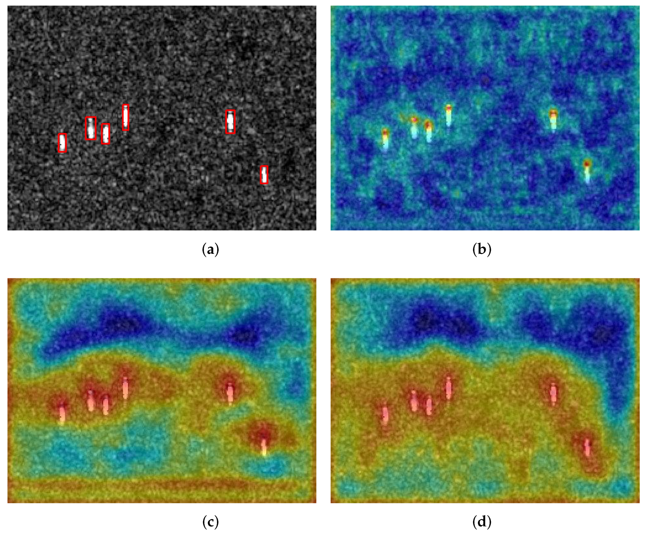
Figure 15.
Visualization of the confidence maps. (a) Ground truth. (b) Visualization of the baseline. (c) Visualization without non-local in WCFF. (d) Visualization with non-local in WCFF.
Figure 15.
Visualization of the confidence maps. (a) Ground truth. (b) Visualization of the baseline. (c) Visualization without non-local in WCFF. (d) Visualization with non-local in WCFF.
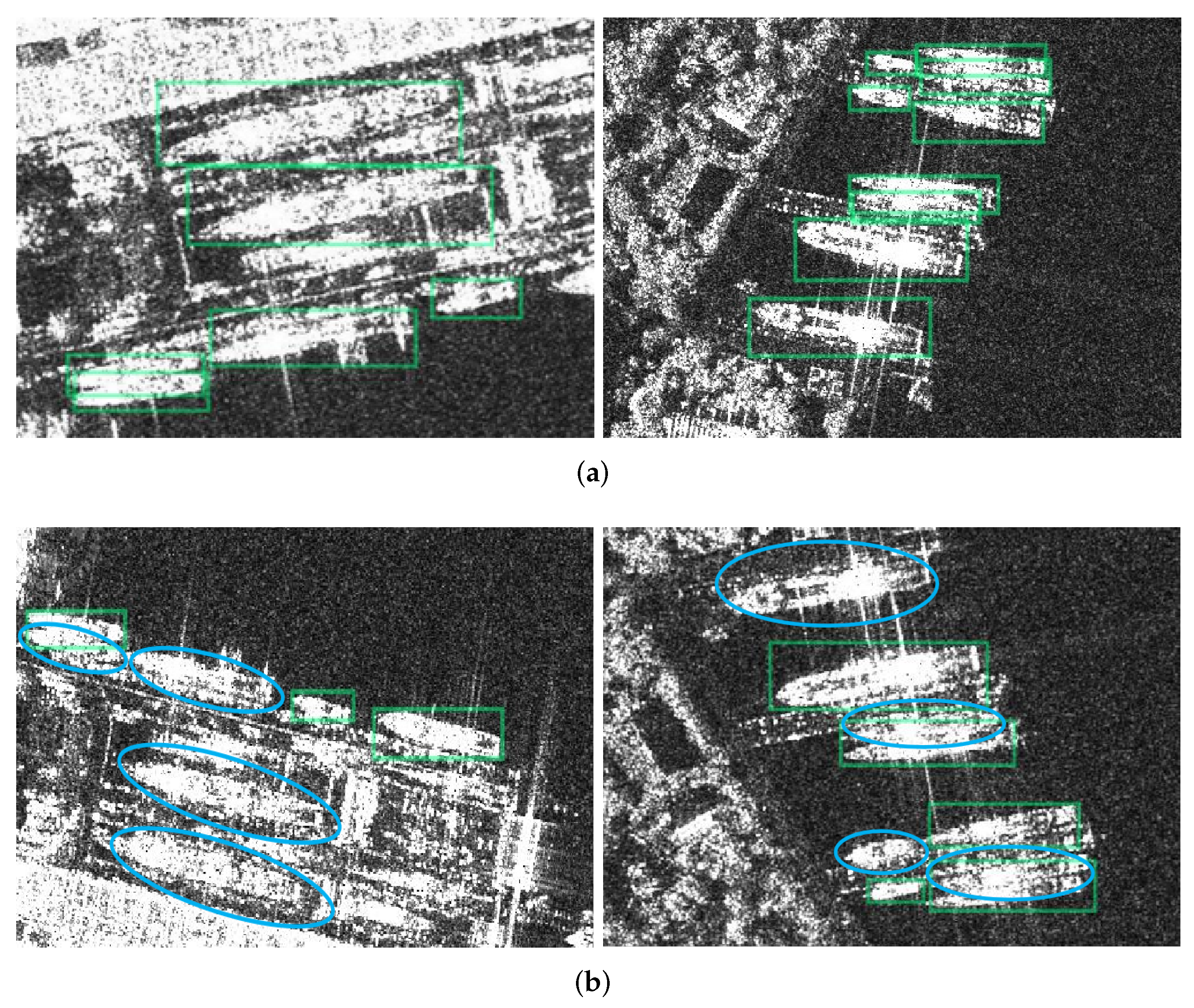
Figure 16.
Comparison detection results of angle-transformed SAR images. The spring-green rectangles represent the detection results. The blue circles represent the missing ships. (a) Satisfactory results. (b) Undesirable results.
Figure 16.
Comparison detection results of angle-transformed SAR images. The spring-green rectangles represent the detection results. The blue circles represent the missing ships. (a) Satisfactory results. (b) Undesirable results.
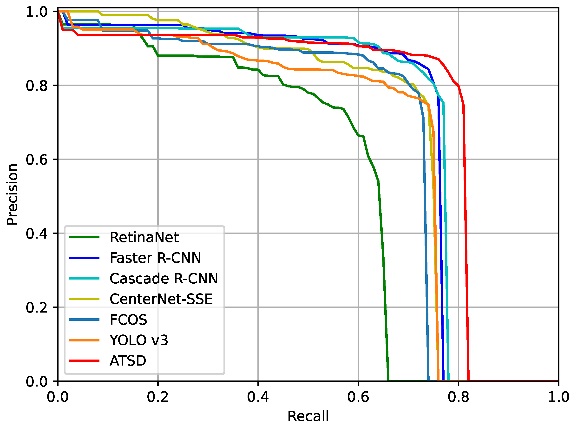
Figure 17.
PR curves of different CNN-based methods under the IoU threshold of 0.75 on the SSDD dataset.
Figure 17.
PR curves of different CNN-based methods under the IoU threshold of 0.75 on the SSDD dataset.
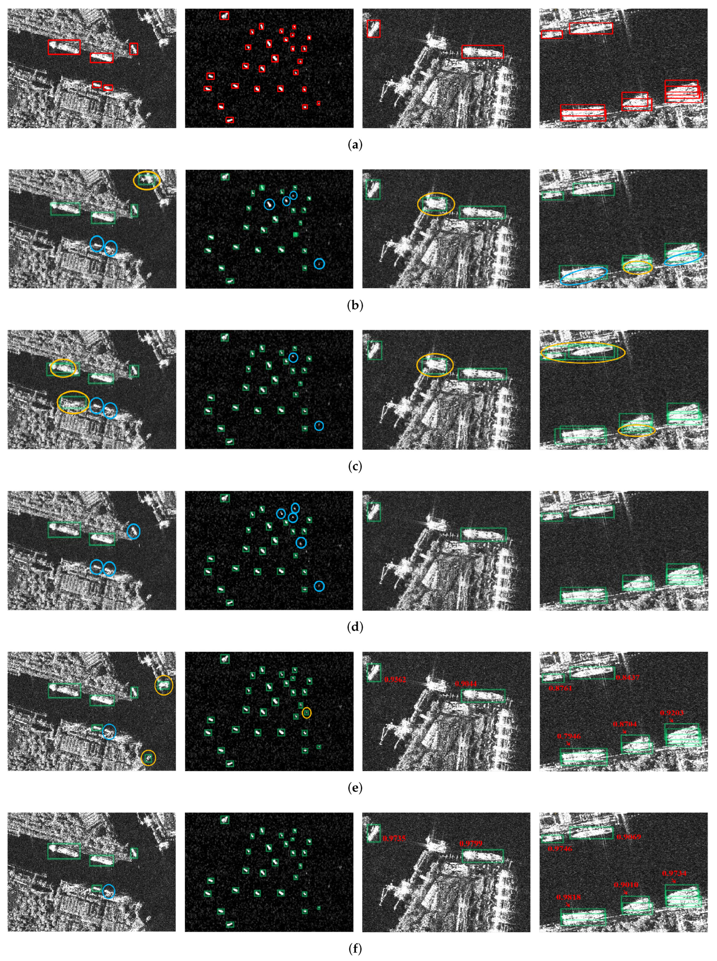
Figure 18.
Comparison results of different methods on the SSDD dataset. The spring-green rectangles are the detection results. The blue and orange circles represent the missing ships and false alarms, respectively. The red value reflects the IoU between the predicted bounding box and the corresponding ground truth. (a) Ground truth. (b) Results of RetinaNet. (c) Results of Faster R-CNN. (d) Results of Cascade R-CNN. (e) Results of CenterNet-SSE. (f) Results of our ATSD.
Table 1.
Statistics of SSDD and HRSID datasets.
Table 1.
Statistics of SSDD and HRSID datasets.
| Dateset | Images | Satellite | Polarization | Resolution (m) |
|---|
| SSDD | 1160 | TerraSAR-X Sentinel-1 RadarSat-2 | HH, VV, VH, HV | 1–10 |
| HRSID | 5604 | TerraSAR-X Sentinel-1B TanDEM | HH, VV, HV | 0.5–3 |
Table 2.
Performance of anchor-based RPN and anchor-free detector (AFD) in two-stage detectors on the SSDD dataset.
Table 2.
Performance of anchor-based RPN and anchor-free detector (AFD) in two-stage detectors on the SSDD dataset.
| Method | AP | AP | AP | Runtime (ms) |
|---|
| RPN-SH | 0.5956 | 0.9137 | 0.7099 | 24.9 |
| RPN-CH | 0.6132 | 0.9301 | 0.7152 | 37.6 |
| AFD | 0.5941 | 0.9522 | 0.6755 | 15.2 |
| AFD-SH | 0.6089 | 0.9567 | 0.7049 | 16.5 |
| AFD-CH | 0.6174 | 0.9597 | 0.7188 | 23.1 |
Table 3.
Performance of each feature enhancement module in our ATSD on the SSDD dataset.
Table 3.
Performance of each feature enhancement module in our ATSD on the SSDD dataset.
| SIA | WCFF | Precision | Recall | F1 | AP | AP | AP | AP | AP | AP | Params (M) |
|---|
| ✕ | ✕ | 0.9455 | 0.9305 | 0.9380 | 0.6174 | 0.9597 | 0.7188 | 0.5837 | 0.6656 | 0.5956 | 61.4 |
| ✓ | ✕ | 0.9693 | 0.9404 | 0.9546 | 0.6225 | 0.9638 | 0.7366 | 0.5766 | 0.6881 | 0.6219 | 61.6 |
| ✕ | ✓ | 0.9482 | 0.9444 | 0.9463 | 0.6255 | 0.9619 | 0.7202 | 0.5853 | 0.6793 | 0.6283 | 61.3 |
| ✓ | ✓ | 0.9695 | 0.9484 | 0.9588 | 0.6373 | 0.9688 | 0.7435 | 0.5976 | 0.6866 | 0.6394 | 61.5 |
Table 4.
Comparisons of various activation functions in SIA module.
Table 4.
Comparisons of various activation functions in SIA module.
| Activation | AP | AP | AP |
|---|
| ReLU | 0.6269 | 0.9614 | 0.7297 |
| swish [68] | 0.6315 | 0.9617 | 0.7317 |
| h-swish [63] | 0.6225 | 0.9638 | 0.7366 |
Table 5.
The comparison results with SENet, scSE, CBAM, CoAM, CoordAtt and our SIA.
Table 5.
The comparison results with SENet, scSE, CBAM, CoAM, CoordAtt and our SIA.
| Method | Precision | Recall | F1 | AP | AP | AP | Params (M) |
|---|
| Baseline | 0.9455 | 0.9305 | 0.9380 | 0.6174 | 0.9597 | 0.7188 | 61.4 |
| +SENet [36] | 0.9520 | 0.9444 | 0.9482 | 0.6172 | 0.9616 | 0.7241 | 61.6 |
| +scSE [54] | 0.9653 | 0.9384 | 0.9517 | 0.6203 | 0.9507 | 0.7243 | 62.2 |
| +CBAM [37] | 0.9412 | 0.9543 | 0.9477 | 0.6196 | 0.9611 | 0.7283 | 61.5 |
| +CoAM [55] | 0.9613 | 0.9384 | 0.9497 | 0.6177 | 0.9609 | 0.7226 | 61.7 |
| +CoordAtt [38] | 0.9556 | 0.9384 | 0.9469 | 0.6189 | 0.9618 | 0.7329 | 61.7 |
| +SIA | 0.9693 | 0.9404 | 0.9546 | 0.6225 | 0.9638 | 0.7366 | 61.6 |
Table 6.
Effectiveness of the non-local network in WCFF module.
Table 6.
Effectiveness of the non-local network in WCFF module.
| Non-Local | Precision | Recall | F1 | AP | AP | AP | Params (M) |
|---|
| ✕ | 0.9573 | 0.9345 | 0.9457 | 0.6201 | 0.9609 | 0.7161 | 60.5 |
| ✓ | 0.9482 | 0.9444 | 0.9463 | 0.6255 | 0.9619 | 0.7202 | 61.3 |
Table 7.
Results of varying the output channels and iterations of WCFF blocks.
Table 7.
Results of varying the output channels and iterations of WCFF blocks.
| #channels (D) | #iterations (N) | AP | AP | AP | Params (M) |
|---|
| 160 | 3 | 0.6194 | 0.9595 | 0.7114 | 44.3 |
| 160 | 4 | 0.6195 | 0.9555 | 0.7129 | 44.6 |
| 256 | 3 | 0.6255 | 0.9619 | 0.7202 | 61.3 |
| 256 | 4 | 0.6240 | 0.9597 | 0.7245 | 61.4 |
Table 8.
Analysis of different values of top-k in the first stage.
Table 8.
Analysis of different values of top-k in the first stage.
| Top-k | AP | AP | AP |
|---|
| 16 | 0.6032 | 0.9316 | 0.7049 |
| 32 | 0.6112 | 0.9514 | 0.7121 |
| 64 | 0.6162 | 0.9597 | 0.7133 |
| 128 | 0.6174 | 0.9597 | 0.7188 |
| 256 | 0.6177 | 0.9597 | 0.7187 |
| 512 | 0.6178 | 0.9597 | 0.7190 |
| 1000 | 0.6184 | 0.9597 | 0.7190 |
Table 9.
Comparison results of CNN-based detectors on the SSDD dataset on various AP metrics.
Table 9.
Comparison results of CNN-based detectors on the SSDD dataset on various AP metrics.
| Method | AP | AP | AP | AP | AP | AP |
|---|
| RetinaNet | 0.5167 | 0.8934 | 0.5500 | 0.4533 | 0.6024 | 0.5014 |
| Faster R-CNN | 0.5956 | 0.9137 | 0.7099 | 0.5447 | 0.6634 | 0.6217 |
| Cascade R-CNN | 0.6132 | 0.9301 | 0.7152 | 0.5779 | 0.6708 | 0.6325 |
| CenterNet-SSE | 0.6043 | 0.9607 | 0.6859 | 0.5405 | 0.6818 | 0.6040 |
| FCOS | 0.5841 | 0.9433 | 0.6645 | 0.5480 | 0.6436 | 0.5034 |
| YOLO v3 | 0.5790 | 0.9492 | 0.6619 | 0.5557 | 0.6210 | 0.5407 |
| Ours | 0.6373 | 0.9688 | 0.7435 | 0.5976 | 0.6866 | 0.6394 |
Table 10.
Comparison results of CNN-based detectors on the SSDD dataset on other metrics.
Table 10.
Comparison results of CNN-based detectors on the SSDD dataset on other metrics.
| Method | Precision | Recall | F1 | Params (M) | FLOPs (G) | Runtime (ms) |
|---|
| RetinaNet | 0.8523 | 0.8591 | 0.8557 | 36.9 | 1.59 | 23.4 |
| Faster R-CNN | 0.9410 | 0.9186 | 0.9297 | 31.8 | 10.51 | 24.9 |
| Cascade R-CNN | 0.9324 | 0.9305 | 0.9314 | 59.6 | 35.27 | 37.6 |
| CenterNet-SSE | 0.9584 | 0.9146 | 0.9360 | 19.8 | 1.39 | 18.2 |
| FCOS | 0.9445 | 0.9126 | 0.9283 | 31.8 | 4.17 | 19.1 |
| YOLO v3 | 0.9282 | 0.9246 | 0.9264 | 61.5 | 2.96 | 13.5 |
| Ours | 0.9695 | 0.9484 | 0.9588 | 61.5 | 7.25 | 32.2 |
Table 11.
Comparison results of CNN-based detectors on the HRSID dataset.
Table 11.
Comparison results of CNN-based detectors on the HRSID dataset.
| Method | Precision | Recall | F1 | AP | AP |
|---|
| RetinaNet | 0.8433 | 0.8034 | 0.8229 | 0.5850 | 0.8450 |
| Faster R-CNN | 0.8685 | 0.8571 | 0.8628 | 0.6301 | 0.8781 |
| Cascade R-CNN | 0.8906 | 0.8579 | 0.8740 | 0.6678 | 0.8740 |
| CenterNet-SSE | 0.8988 | 0.8360 | 0.8663 | 0.6178 | 0.8748 |
| FCOS | 0.8957 | 0.8328 | 0.8631 | 0.6027 | 0.8730 |
| YOLO v3 | 0.8298 | 0.8809 | 0.8546 | 0.6055 | 0.8712 |
| Ours | 0.9026 | 0.8656 | 0.8837 | 0.6726 | 0.8819 |


