Abstract
Semantic segmentation of remote sensing images plays a crucial role in urban planning and development. How to perform automatic, fast, and effective semantic segmentation of considerable size and high-resolution remote sensing images has become the key to research. However, the existing segmentation methods based on deep learning are complex and often difficult to apply practically due to the high computational cost of the excessive parameters. In this paper, we propose an end-to-end lightweight progressive attention semantic segmentation network (LPASS-Net), which aims to solve the problem of reducing computational costs without losing accuracy. Firstly, its backbone features are based on a lightweight network, MobileNetv3, and a feature fusion network composed of a reverse progressive attentional feature fusion network work. Additionally, a lightweight non-local convolutional attention network (LNCA-Net) is proposed to effectively integrate global information of attention mechanisms in the spatial dimension. Secondly, an edge padding cut prediction (EPCP) method is proposed to solve the problem of splicing traces in the prediction results. Finally, evaluated on the public datasets BDCI 2017 and ISPRS Potsdam, the mIoU reaches 83.17% and 88.86%, respectively, with an inference time of 0.0271 s.
1. Introduction
Due to the rapid development of remote sensing equipment and technology, the amount and ease of access to spatial data have significantly increased. How to interpret large-size and high-resolution remote sensing images automatically, quickly, and efficiently has become a hot issue for research. Among them, the semantic segmentation of remote sensing images plays a vital role in urban planning [1,2,3,4,5], environmental monitoring [6,7,8,9,10], forest and crop analysis [11,12,13,14,15], and smart city construction [16,17,18,19,20].
Semantic segmentation for remote sensing imagery aims to interpret the ground content of the image and obtain its pixel-level semantic annotation [21]. The segmentation tasks usually focus on extracting single or multiple categories, such as buildings [22], roads [23], the vegetation [24], etc. However, due to the complex and diverse information these categories possess, the richness of features and the varying scale sizes pose a significant challenge to the semantic segmentation of remote sensing images.
Traditional image processing methods cope with the task of semantic segmentation of remote sensing images mainly by extracting color, grayscale, geometric features, etc., such as the extraction of water body information from Landsat ETM+ images using Ada-Boost algorithm [25] and a multi-scale building extraction method based on mathematical morphology [26]. These manually designed feature extractors are relatively complex and challenging to adapt to complex application scenarios with limited generalization capability. In recent years, the fire of deep learning methods, especially convolutional neural networks (CNNs), has gradually replaced the traditional techniques in various computer vision tasks. Undoubtedly, new research directions have also opened up in the semantic segmentation of remote sensing images.
The critical advantage of CNN-based algorithms is that they provide an end-to-end solution for image detection, where the ability to generalize is greatly improved by replacing the manually designed feature layers with autonomous feature learning methods. For example, building fully connected networks (FCNs) combine deep and shallow information to produce accurate segmentation results [27]. However, FCNs lose much information during upsampling because they do not consider the progressive relationship between pixels; so, SegNet [28], which performs nonlinear upsampling using pooling indexes, was proposed. This architecture is well-suited for scene-understanding applications and has good accuracy. Based on this idea, U-Net [29], symmetric path networks have also achieved good semantic segmentation results. Although these networks have significant consequences for category segmentation, they lack detail processing capability due to insufficient use of context. To address this limitation, Chen et al. proposed a DeepLabv3+ network using atrous convolution and atrous spatial pyramid pooling (ASPP) [30], which captures objects and links images at multiple scales. The contextual approach can robustly segment object classes while representing the detailed information of the target well.
However, all these networks are very complex, and the number of parameters is huge when applied to the semantic segmentation of remote sensing images, which inevitably brings the problem of increasing computational cost. The remote sensing images may vary significantly in terms of feature points due to factors, such as climate change, regional topography, water quality, vegetation types, and even different styles of architecture. Therefore, the models designed for semantic segmentation of remote sensing images should be as lightweight as possible so that prediction results can be obtained as soon as possible at a low cost in the face of changing environments.
Since lightweight networks have a limited ability to extract features compared to deep models, how to perform automatic, fast, and effective semantic segmentation of very high-resolution remote sensing images without reducing accuracy becomes the purpose of our research.
The flow chart of this paper’s proposed remote sensing image segmentation system is shown in Figure 1. Step 1 involves cropping the edge padding high-resolution remote sensing, Step 2 involves predicting the small-segmented images sequentially using the proposed LPASS-Net, and Step 3 involves stitching the predicted results together and restoring them.
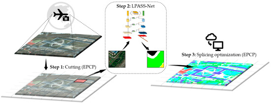
Figure 1.
Flowchart of the proposed large-size and high-resolution remote sensing image semantic segmentation system.
The main contributions of this paper are as follows:
- A lightweight progressive attention semantic segmentation network (LPASS-Net) is proposed, which utilizes an efficient, lightweight backbone network, atrous spatial pyramid pooling (ASPP) modules, and reverse progressive attention. Using an enhanced feature fusion network, the algorithm improves its robustness when segmenting targets of different scales and solves the problem of local information loss. In contrast, the design of the feature fusion network can enrich the diversity of features of each discipline, which is conducive to improving the accuracy of segmentation when size and perspective change phenomena.
- The proposed lightweight non-local convolutional attention network (LNCA-Net) is a spatial dimensional attention mechanism that breaks the limitation of only local feature integration by an improved autocorrelation matrix operation.
- An edge padding cut prediction (EPCP) is proposed to segment and splice images by the edge padding method, which can well solve the problem of producing splice traces when direct prediction is performed.
2. Related Work
Most deep-learning semantic segmentation models are based on an encoder–decoder architecture. The encoder uses convolutional and pooling layers to reduce the feature map size to obtain a feature map. The decoder projects the acquired feature semantics onto a high-resolution pixel space to obtain a dense classification. SegNet and U-Net are representative encoder–decoder architectures, where SegNet’s network design uses nonlinear upsampling in the decoder stage to reduce the number of parameters needed during training. U-Net consists of a systolic path for collecting context and an extended symmetric path for identifying precise locations. This structure allows features to be stitched together in the channel dimension to form richer features, efficiently performing semantic segmentation even with few training images. In recent research, many researchers have worked on improving the fused attention mechanism for semantic segmentation of remote sensing images.
For example, Ref. [31] proposed a fused sparse channel attention (SCA)-based UNet dual stream branching model (DF-UNet) with segmentation and ranking branches for detecting different levels of wheat yellow rust in remote sensing images. Ref. [32] proposed inserting channel spatial attention (CSA) in the fused encoder and decoder features to detect particular types of unauthorized buildings. Ref. [33] proposed a remote sensing urban scene image segmentation model based on ResNet18 as the encoder and transformer as the decoder and developed an efficient attention mechanism to model global and local information in the decoder. Ref. [34] proposed to improve the U-Net model using two attention mechanisms, ECA-Net and PSA-Net, aiming to segment important details in wind turbines from images captured by remote sensing. Ref. [35] proposed an attention-augmented convolution-based residual UNet architecture (AA-ResUNet) for road extraction in remote sensing images, where the attention-enhanced convolution operation helps to capture remote global information and obtain a more discriminative feature representation. These works are used to improve the segmentation efficiency by modifying the model structure by incorporating attention mechanisms.
By contrast, many works have focused on weighting the features at each pixel location to improve the segmentation efficiency. For example, Ref. [36] proposed a novel bottleneck structure operation to optimize DeepLabv3+, which uses operations, such as reweighting and summation by the attention mechanism, to make the features of essential regions in the image more significant, improving the expressive power of the convolutional neural network, and better solving the problem of coarse boundaries in semantic segmentation. A sense-global-entropy network (DGEN) is proposed by [37], which introduces a dual local and global attention mechanism to embed it into densely connected convolutional networks (DenseNets) to preserve the integrity of segmentation. Ref. [38] embedded a channel-attention mechanism in a multi-scale adaptive feature fusion network (MANet) to fuse semantic features. High-level and low-level semantic information is connected by global average pooling to generate global features for semantic segmentation in remote sensing images.
However, most methods only consider segmentation accuracy and ignore the limitation of an excessive number of parameters due to the complexity of the model itself. In this paper, we propose an efficient and a robust semantic segmentation network named LPASS-Net to address the limitations of previous studies. The rationality and superiority of the method are demonstrated in a series of ablation experiments using two publicly available datasets, which help to promote the development of remote sensing image processing applications and provide new ideas for lightweight research of neural networks.
3. Methodologies
The overall architecture of our proposed LPASS-Net is shown in Figure 2, which consists of three main parts: a backbone feature extraction network part based on MobileNetv3, an ASPP module and an enhanced feature extraction network part consisting of a RPA-Net, and finally, a prediction network part. Notably, we propose a modified LNCA-Net, which constitutes a reverse progressive attentional feature fusion structure by gradually adding this attentional module to enrich the diversity of feature layers and adaptively adjust the attention of the network.
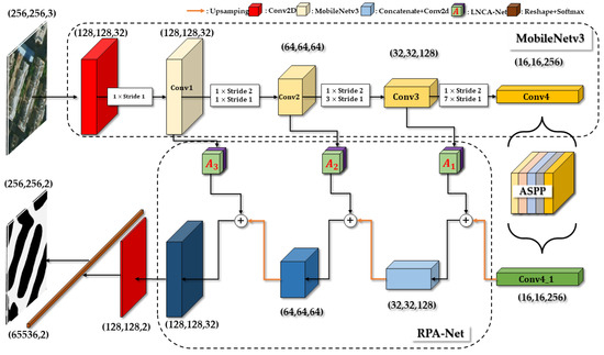
Figure 2.
The network framework of the LPASS-Net is proposed in this paper.
Firstly, since the number of parameters in the backbone network directly determines the overall parameter size of the model, MobileNetv3 was used as the backbone network for feature extraction to meet the overall lightweight network. In addition to the four adequate feature layers obtained using the backbone network, the final feature layer Conv4 had a shape of (16, 16, 256) and was connected to an ASPP module with five parallel branches. To enhance the expressiveness of the feature map and facilitate the detection of targets at different scales, null convolution was used to achieve local and global feature fusion. Secondly, the reinforced feature layers of the ASPP module were used for reverse progressive upsampling. Combining with the attention mechanism LNCA-Net, the feature fusion and upsampling were performed gradually with the remaining three feature layers in the backbone network to obtain the final feature layer with all fused features. Finally, this feature layer was used to classify each feature point, equivalent to the predictive classification of each pixel point, to form the predictive output module.
3.1. Lightweight and Efficient Backbone Network
For deep learning algorithms designed for semantic segmentation problems applied to high-resolution remote sensing images, it is especially critical that the network itself is lightweight and efficient due to the memory and power constraints of the application device. The problem of how to make the network computationally reduced while ensuring accuracy has received widespread attention, of which the MobileNet series is excellent, whereas MobileNetV3 [39], after the accumulation of the first two generations of V1 [40] and V2 [41], utilizes the deep separable convolution of MobileNetV1 while synthesizing MobileNetV2 with linear bottleneck and a squeeze-and-excitation network (SE-Net) [42] of the inverse residual structure. The overall computation of the neural network mainly depends on the number of parameters of the backbone network, so it is essential to choose a lightweight backbone network. In this paper, the B-neck structure of MobileNetV3 was used as the backbone network by concatenating, as shown in Figure 3, to improve the execution speed of the network.
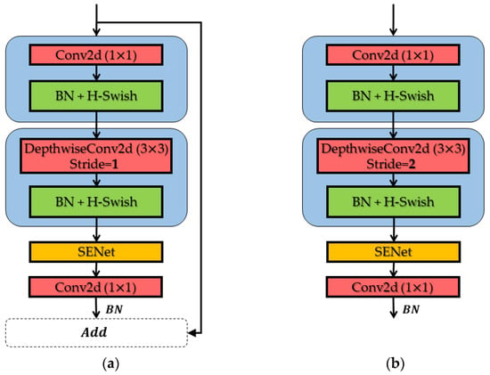
Figure 3.
The structure of two backbone network modules: (a) Stride 1 and (b) Stride 2, respectively.
The B-neck was composed of an inverted residual block, first using 1 × 1 standard convolution to up-dimension and then extracting features by depthwise separable convolution, using SE-Net attention mechanism, and finally using 1 × 1 standard convolution to down-dimension and output. This design allowed less information to be lost when high-dimensional information was passed through the activation function. In addition, the B-neck was divided into two structures according to the step size. The shortcut connection was only available when the stride was 1, i.e., when the input features had the same shape as the output features. We constructed the feature extraction backbone network in Figure 2 by combining two kinds of B-neck.
The feature extraction process used a preliminary feature map obtained by one standard convolution first, followed immediately by each feature layer being compressed and deepened by combining one Stride 2 and multiple Stride 1s. A total of four feature layers, namely Conv1, Conv2, Conv3, and Conv4, were obtained with shapes of (128, 128, 32), (64, 64, 64), (32, 32, 128), and (16, 16, 256), respectively. These preliminary feature layers needed to be processed through an enhanced feature extraction network to deepen the sampling capability of the model to deepen the model’s sampling capability for features.
3.2. Enhanced Feature Extraction Network
The enhanced feature extraction network proposed in this paper aimed to increase the richness of the feature map and was composed of an ASPP module and a reverse progressive attention feature fusion network. The ASPP module evolved from the spatial pyramid pooling (SPP) module [43]. It aimed to sample features by convolution kernels at different scales, enabling accurate and efficient classification of regions at arbitrary scales. This method of fusing local and global feature information can enhance the correlation between features in the spatial dimension. However, using pooling layers alone in SPP to increase the perceptual field also decreased the resolution and led to the loss of detailed information. To solve this problem, one can use null convolution instead of pooling layers to achieve a larger perceptual field while reducing the loss of resolution [44].
The ASPP module shown in Figure 4 has five branches, the first three use a 3 × 3 atrous convolution with convolution kernels and rates of 6, 12, and 18, respectively. The last two branches will use a standard convolution with a 1 × 1 kernel, the difference being whether or not they pass through the global average pooling layer. The features of each branch are then merged to obtain a Conv4_1 of the shape (16, 16, 256) by compressing the number of channels using the standard convolution of 1 × 1. The structure of an atrous convolution with different rates in parallel is often used in semantic segmentation because it can increase the perceptual field and capture multi-scale information without increasing the number of parameters. However, the pixel points generated by the nature of the atrous convolution are disjointed, and they are independent of each other lacking dependencies, which can cause local information loss and no correlation between features at a distance. Therefore, the latter two branches of the ASPP module proposed in this paper were designed to compensate for this drawback by enhancing the global and local information interaction through global average pooling and standard convolution with a 1 × 1 convolution kernel.
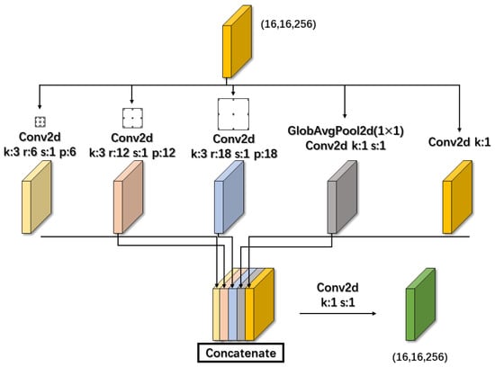
Figure 4.
The structure of the atrous spatial pyramid pooling (ASPP).
Since there are targets of different sizes in the semantic segmentation of high-resolution remote sensing images, even though the feature layer Conv4 of the backbone feature extraction network can obtain feature layers with high semantic information after processing by the ASPP module, its size is small, compared with other feature layers of larger sizes, which still retain rich feature details. More feature layers need to be combined to improve the accuracy of the results. However, blind direct upsampling for the concatenated merging of multiple feature layers is flawed due to the interference of redundant details in the background for detection.
It becomes necessary to use an attention mechanism to weigh the features at all pixel locations for each size. As shown in the RPA-Net of Figure 2, each backbone feature layer was attentionally enhanced and then combined with the previous feature layer that was upsampled so that a gradual reverse progression of decoding allowed more features to be generated for semantic segmentation.
The core idea of the attention mechanism was to let the model learn to focus on the critical information and ignore the unimportant information, which was to understand the weight distribution by using the relevant feature map and then apply the obtained weights to the original feature map, to sum up, the weights. The weighting can be applied to the spatial domain to transform the information in the spatial part of the image to extract the critical data. It can also be used in the channel domain, adding a weight to each channel signal to represent the channel’s relevance to the necessary information; the more significant the importance, the higher the relevancy.
In our previous work, we proposed the lightweight residual convolutional attention network (LRCA-Net) [45], which is spatial-channel hybrid attention, with the core idea of improving the channel attention module of CBAM [46] by using 1D convolution instead of fully connected layers and adding a residual structure. Such an improvement can improve the performance a lot, but it does not improve the spatial attention module, as shown in Figure 5.
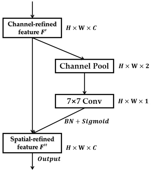
Figure 5.
The spatial attention module of the LRCA-Net.
The spatial attention module pools the input features with the shape of C × H × W by the maximum and average pooling and then connects the two obtained features into a channel pool with the shape of 2 × H × W and convolves them by a standard convolutional layer of size 7 × 7 to obtain the spatial attention map by sigmoid as in Equation (1).
where As denotes the spatial attention module, F′ denotes the channel refined feature, σ denotes the sigmoid function, and k7×7 represents the convolution of kernel size 7 × 7.
By analyzing it, it can be seen that the drawback of such a spatial attention module is very obvious because simply performing a 7 × 7 convolution is limited by the size of the convolution kernel, which is only limited to the features of adjacent points that can be captured by the convolution and lacks the remote interaction between any two more distant positions; so, how to use the attention structure in the spatial dimension to effectively integrate global information by performing autocorrelation on the global feature map has become the direction of this improvement.
Non-local neural networks provide an autocorrelation matrix algorithm for the problem of how to capture long-range dependencies [47]. Along this line, we improved the spatial attention module, as shown in Figure 6. First, we generated three copies of the input feature maps F′ of shape H × W × C by standard convolution of 1 × 1, respectively, and reshaped them into N × C, where N is equal to H × W, as in Equation (2).
where Conv2d represents the convolution kernel as a 1 × 1 standard convolution operation, reshape is the reshaping function, and the shapes of R1, R2, and R3 are N × C, where N is equal to H × W.
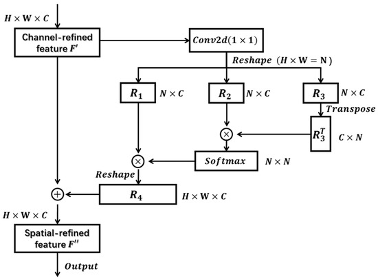
Figure 6.
The structure of the spatial attention module is modified by the autocorrelation matrix algorithm.
After transposing R3 to obtain and performing matrix multiplication with R2, using the softmax layer to obtain the spatial attention map, we performed matrix multiplication with R1 and reshaped it to obtain R4 with the shape H × W × C as in Equation (3), and finally added R4 to the input feature map F′ to obtain the spatial-refined feature F″ as in Equation (4).
where represents the transpose matrix of R3, S represents the softmax function, and F″ represents the spatial-refined feature.
In contrast to the previous spatial attention module, performing the standard convolution operation involved only a weighted sum of the pixel values around that location. In contrast, by an improved autocorrelation matrix operation, finding a value at a location corresponded to a weighted sum of the values at all locations. For the features at a specific location, the features at all locations were aggregated and updated by a weighted sum, where the weights were determined by the similarity of the features at the corresponding two locations. Therefore, the implementation of non-local attention that associated the features between two pixels at a certain distance on the image helped the network model accomplish the semantic segmentation task; an illustration of the dependencies of the global context information compared to the local information is shown in Figure 7.
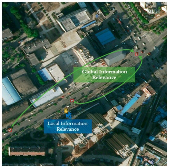
Figure 7.
Global and local information dependencies. Local dependencies are presented by convolution (yellow). The long-distance boxes (red) present the global dependencies.
With replacement of the previous method with a proposed spatial attention module, the overall structure of the improved attention mechanism LNCA-Net was obtained, as shown in Figure 8. Since the network design without changing the feature map size allowed LNCA-Net to be inserted into arbitrary network structures, the progressive attentional feature fusion structure was designed in combination with such an attention mechanism.

Figure 8.
The overall structure of the lightweight non-local convolutional attention network (LNCA-Net) contains the original channel attention mechanism Ac and the modified channel attention mechanism As.
Image conversion from low- to high-resolution images can lead to distortion. Using the skip connection structure to combine the distortions was relatively negligible and retained more detailed information. Such a progressive feature fusion structure can directly connect gradient, point, line, and other input to the decoder more accurately after the attention enhancement process of the same shape feature layer in the encoder, which is equivalent to adding more detailed information when judging the target region, which is beneficial to obtain more accurate segmentation results.
3.3. Splicing Optimization Method
Due to the high resolution and large size of the directly captured remote sensing images, they cannot be directly input into the network. For this reason, we have designed a cut-and-predict method, the core of which is to divide the original image into several small pieces of the same size and then input them into the network for prediction and stitching. Stitching the prediction results directly will produce stitching traces because of the boundary feature extraction, which will affect the final output. To solve this problem, we needed to perform edge filling on the original image when segmenting it, as in Figure 9.
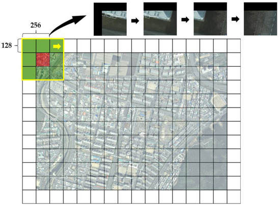
Figure 9.
Example of the edge padding cutting operation.
The main idea of EPCP is to segment a sliding window of each region that covers the center patch and its 8 neighboring patches and to keep only the center part of the image for each prediction, and the rest part is discarded. Then, the discarded part will also become the center part of the following prediction using the sliding window. This method avoids the problem of feature extraction of the border and the splicing trace, which affects the final segmentation effect. For example, suppose the center patch size is 128 × 128, the step size is set to 128, and it moves to the right in the form of a sliding window.
3.4. Experiments
In this section, we first introduced the dataset and experimental environment used. Then, we described the model training setup and evaluation metrics, and finally, we evaluated the reliability of our proposed method by analyzing and discussing the experimental results.
3.4.1. Dataset and Experimental Environment
We conducted experiments on two remote sensing datasets with different styles, as shown in Figure 10, the Big Data and Computing Intelligence Contest 2017 (BDCI 2017) dataset and the International Society for Photogrammetry and Remote (ISPRS) Potsdam dataset. The BDCI 2017 dataset provides a total of four remote sensing images of water towns in China, with corresponding annotated images, which are annotated into five categories: vegetation, buildings, water bodies, roads, and others, among which cultivated land, forest land, and grassland are classified as vegetation. In contrast, ISPRS Potsdam shows a typical historical city with giant building blocks, narrow streets, and dense settlement structures. We used eight pairs of these remote sensing images with their corresponding ground annotated images for the experiment, and their annotations were classified into six categories: impervious surfaces, buildings, low vegetation, trees, cars, and clutter.
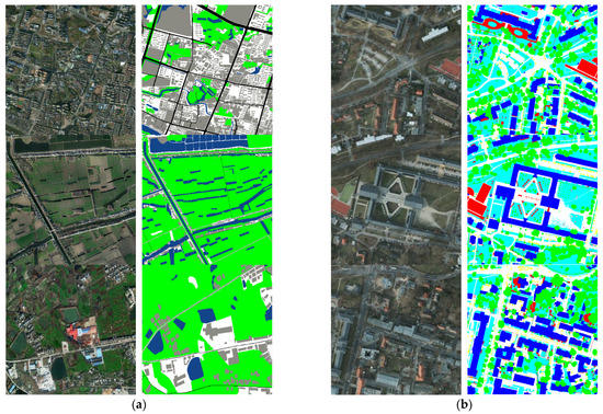
Figure 10.
Examples of original and annotated images of two different styles of remote sensing datasets used for the experiments in this paper: (a) the BDCI 2017 dataset and (b) the ISPRS Potsdam dataset, respectively.
To facilitate deep learning of the network model, we obtained more diverse data samples by data augmentation. In this study, we first needed to cut the remote images in the two datasets to scale each image to 256 × 256. Then, we used rotation, mirroring, color transformation, and Gaussian filtering to enrich the diversity of the data samples and finally obtained 100,000 training data, respectively, where each training and validation set was randomly divided in the ratio of 9:1 90,000 and 10,000, respectively. Some examples of the original images and labels of the dataset are shown in Figure 11.
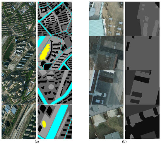
Figure 11.
Representative samples of each category in the dataset after data enhancement of the original images are shown on the left and ground truth on the right: (a) the BDCI 2017 dataset and (b) the ISPRS Potsdam dataset.
The experimental setup of this study is shown in Table 1. An RTX 3050 graphics card was paired with an Intel(R) Core (TM) i5–11400F processor to form a high-performance workstation. TensorFlow2 was used to build the experimental models for training, validation, and testing, and CUDA was used to compute the results.

Table 1.
Mainframe hardware and software for workstations.
3.4.2. Evaluation Metrics and Experimental Details
To verify the accuracy of the network, we used the following metrics to evaluate the model. Semantic segmentation tasks usually combined precision and recall to evaluate the results as in Equations (5) and (6). The mean intersection over union (mIoU) and F1-score were chosen to evaluate the overall results as in Equations (7) and (8); the larger these values are, the higher the agreement of the predicted results with the ground truth. These indicators are calculated as follows:
where T/F denotes true/false, which indicates whether the prediction is correct, and P/N denotes positive/negative, which indicates a positive or negative prediction result.
where TPc, FPc, and FNc denote true positives, false positives, and false negatives of a particular object indexed to class C, respectively.
4. Results and Discussion
To verify the rationality and effectiveness of LPASS-Net, we designed ablation experiments to explore the effect of the execution of different combinations of modules in the network on the results. As a fair comparison, except for the parameters of the added modules, such as the dataset (ISPRS Potsdam dataset), input image size, relevant hyperparameters, training strategy, and experimental environment, they are the same in the ablation experiments. As shown in Table 2, when the original base algorithm (baseline) uses only the end feature layer extracted by the backbone network for upsampling reduction and outputs the results without adding any module, the mIoU is only 73.50%. After adding the ASPP module, the mIoU improves significantly to 76.11%, and after adding the progressive attention network, the results improve to 83.17%. These ablation experiments show that the proposed network module can effectively improve the segmentation accuracy when performing segmentation tasks.

Table 2.
Results of ablation experiments using the same dataset (BDCI 2017), where bold numbers indicate the highest mIoU, “√” indicates that the leftmost component is used in the model, and “×” indicates that the leftmost component is removed. In each column, the last number represents the mIoU obtained using the corresponding component.
To validate our improved attention mechanism, we designed ablation experiments for the attention mechanism, the corresponding results are presented in Table 3. They are based on testing of the single model proposed in this paper, with no differences in the network modules used, and with the same dataset, input image size, and associated hyperparameters, where the baseline is set not to add any attention module. The models of all attention methods improve the segmentation results. However, when we used the improved method, better results were achieved using the other attention methods. It is confirmed that the non-local attention method is more effective in integrating global information than the method that performs only standard convolution.

Table 3.
Experiments on the ablation of attentional mechanisms using the same dataset (BDCI 2017), where bold numbers indicate the highest mIoU, “+” indicates that a particular attention module has been added to the baseline.
In addition, to further discuss the necessity of several attentional module configurations in RPA-Net, ablation experiments were designed to verify the effect of the execution method of progressively combining attentional modules on the results. As shown in Table 4, when the original base algorithm (baseline) performs only upsampling reduction and outputs the results without adding the attention module, the mIoU is only 80.91%. After gradually adding the LNCA-Net module, the mIoU increases to 81.51%, 82.47%, and 83.17%, respectively. The results of this ablation experiment demonstrate the rationality of the proposed progressive attention module addition method when performing segmentation tasks.

Table 4.
Results of ablation experiments using the same dataset (BDCI 2017), where bold numbers indicate the highest mIoU and “√” indicates the top component used in the model. In each row, the last number represents the mIoU obtained using the corresponding component.
For the predicted patch image to be stitched directly, it often produces stitching traces as shown in Figure 12. It can be seen that this problem is well solved by the EPCP method proposed in this paper, and the splice traces are substantially reduced and do not affect the segmentation effect.
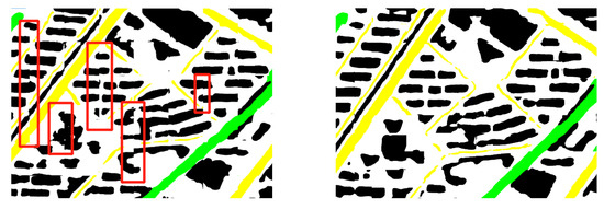
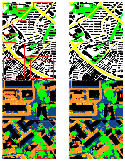
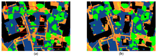
Figure 12.
Examples of the results of two datasets optimized by EPCP, respectively, where the red boxes mark the splice traces: (a) unoptimized results and (b) optimized results.
For a comprehensive evaluation, the LPASS-Net algorithm is compared with representative semantic segmentation models, such as SegNet [28], PSPNet [48], U-Net [29], and DeepLabv3+ [30], to enrich the comparison models by replacing the backbone network.
Figure 13 shows a plot of the loss values during the training of the model and a plot of the validation loss function obtained by validating the model using the validation dataset during the training process. The training is divided into two phases, the freeze phase and the unfreezing phase. The pre-trained MobileNetv3 backbone model was used to initialize the weight parameterization of the underlying shared convolutional layer. The loss function was set to a cross-entropy loss function with training batch sizes of 16 and initial learning rates of 0.001 and 0.0001 for the freeze and thaw phases, respectively. The first 50 epochs freeze the backbone network weights and prioritize the training of network weights other than the backbone network, and the second 50 epochs unfreeze the backbone network for full network training. This has the advantage of fine-tuning the original weights of the backbone network, thus accelerating the convergence of the network and saving training time.
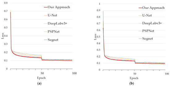
Figure 13.
LPASS-Net training evolution of the loss function on (a) the BDCI 2017 dataset and (b) the ISPRS Potsdam dataset, respectively; the red line represents train loss, and the green line represents validation loss.
The comparison of quantitative experimental results using the same dataset and model training methods is reported in Table 5. The mIoU of our proposed method can reach 83.17% and 88.86% on the BDCI 2017 dataset and ISPRS Potsdam dataset, respectively, and mF1 reaches 89.17 and 94.55, respectively, which is an improvement compared with other segmentation methods.

Table 5.
Comparison of quantitative experimental results on the two datasets, where bold numbers indicate the best value for each column. The first of these numbers is the result from the BDCI 2017 dataset, the second is from the ISPRS Potsdam dataset, and the inferred time is the time required to predict a 256 × 256 patch image.
In practical applications, it is essential to consider not only the efficiency of the model but also the size of the model. As shown in Figure 14, compared to PSPNet (MobileNetv3) with a similar number of parameters, our method improves mIoU by 8.42% and 10.73%, respectively, and F1-score by 10.06% and 9.73% on both datasets. Although these algo-rithms have no shortage of models with high segmentation efficiency, such as DeepLabv3+ (Xception) and PSPNet (ResNet50), our method is not only more accurate compared to them, but the model sizes are only 17.38% and 15.33% of theirs. According to the visualization results in Figure 15 and Figure 16, LPASS-Net segmented buildings’ edges more clearly than other models. The SegNet and U-Net can segment more significant buildings and vehicles, but there are a lot of errors in segmenting small clutters. PSPNet and DeepLabv3+ perform very well in general, but compared with LPASS-Net, the segmentation of low vegetation and trees is not accurate enough. For the time factor, our method takes only 0.0271s to process, which implies a good improvement in processing speed compared to DeepLabv3+ when reaching the same mIoU level. This shows that our proposed LPASS-Net can achieve high segmentation accuracy with a smaller model size.
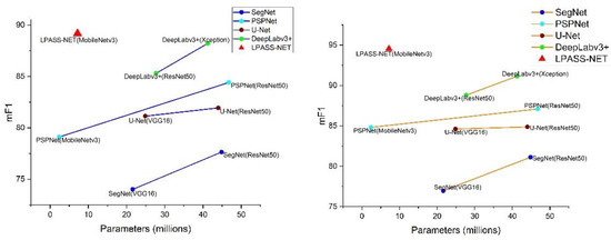
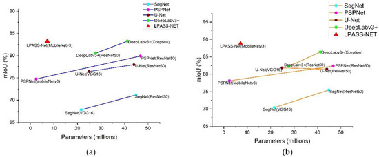
Figure 14.
Model size vs. mIoU and mF1 in (a) the BDCI 2017 dataset and (b) the ISPRS Potsdam dataset. Details are in Table 5. Note that our approach obtains better results while having less model complexity.
After completing the overall evaluation of the models, we use the intersection over the union set as a class evaluation metric. Based on the BDCI 2017 and ISPRS Potsdam da-tasets, Table 6 and Table 7 show the IOU results of different methods.

Table 6.
The results of IOU on the BDCI 2017 dataset of different methods (%), where the bolded numbers indicate the best value for each column.

Table 7.
The results of IOU on the ISPRS Potsdam dataset of different methods (%), where the bolded numbers indicate the best value for each column.
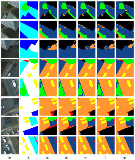
Figure 15.
Examples of segmentation details of different models on the ISPRS Potsdam dataset: (a) original image, (b) ground truth, (c) SegNet, (d) U-Net, (e) PSPNet, (f) Deeplabv3+, (g) LPASS-Net, where the category details are shown in Table 8.

Table 8.
Details of each category in the prediction results.
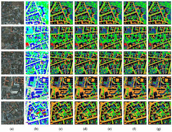
Figure 16.
Examples of full-size output results of different models on the ISPRS Potsdam dataset: (a) original image, (b) ground truth, (c) SegNet, (d) U-Net, (e) PSPNet, (f) Deeplabv3+, (g) LPASS-Net, where the category details are shown in Table 8. In addition, the visualization results of each model are obtained by adding EPCP to ensure the fairness of the ablation experiment.
The experimental visualization results, shown in Figure 17 and Figure 18, show that LPASS-Net can distinguish different feature types and perform very accurately in the boundary detail part. In particular, the segmentation accuracy of vehicles, building clusters, roads, and vegetation is higher than other models. Because LPASS-Net can combine multi-scale semantic information, and when combined with LNCA-Net, which uses an attention mechanism, it can enhance the correlation between pixels and greatly enrich the diversity of features. It confirms the robust segmentation capability of our LPASS-Net, which can be well applied to the semantic segmentation of remote sensing images.
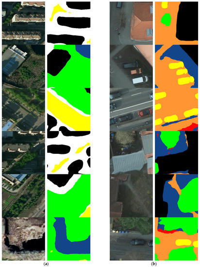
Figure 17.
Prediction details of the test images are provided by LPASS-Net in (a) the BDCI 2017 dataset and (b) the ISPRS Potsdam dataset, where the category details are shown in Table 8.
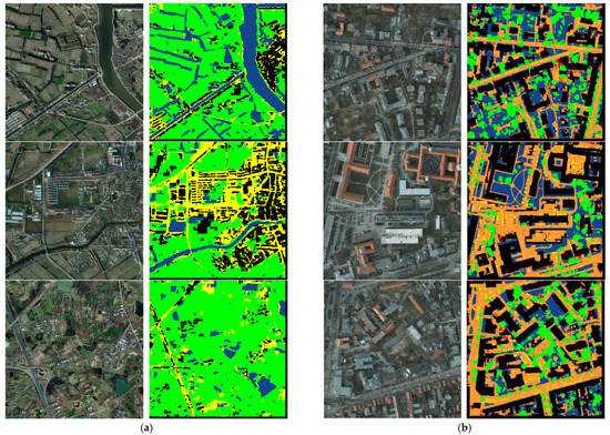
Figure 18.
The overall visualization results of the test images provided by (a) the BDCI 2017 dataset and (b) the ISPRS Potsdam dataset, where the category details are shown in Table 8.
5. Conclusions
To perform automatic, fast, and effective category segmentation of large-size and high-resolution remote sensing images and to solve the problem of reducing computational cost without losing accuracy, an end-to-end LPASS-Net is proposed in this study. Firstly, MobileNetv3 is used as the backbone feature extraction network, which can ensure efficient automatic feature extraction while significantly reducing the overall number of model parameters. Secondly, an enhanced feature extraction network consisting of an ASPP module and a RPA-Net is designed, which can improve the algorithm’s robustness in segmenting targets at different scales. In contrast, the design of the feature fusion network can enrich the diversity of various types of features. Thirdly, based on the shortcomings of the LRCA-Net proposed in previous studies, an improved LNCA-Net is proposed, which can effectively integrate global information in the spatial dimension by performing autocorrelation on the global feature map to improve segmentation performance. Fourthly, the proposed EPCP method is an excellent solution to the problem of splicing traces’ indirect prediction. Finally, evaluated on the public datasets BDCI 2017 and ISPRS Potsdam, the mIoU achieved 83.17% and 88.86%, respectively, and the inference time was 0.0271 s per 256 × 256 patch map, which confirms the superiority of LPASS-Net. This helps to promote the application of algorithms for remote sensing image processing and provides a direction for the research of lightweight neural networks.
Author Contributions
H.L.: Conceptualization, Methodology, Writing—original draft, Software, Formal analysis. S.S.: Supervision, Funding, Writing—review and editing, Resources, Formal analysis. All authors have read and agreed to the published version of the manuscript.
Funding
This research was supported by Basic Science Research Program through the National Research Foundation of Korea (NRF) funded by the Ministry of Education (2016R1D1A1B02011625).
Conflicts of Interest
The authors declare no conflict of interest.
References
- Kampffmeyer, M.; Salberg, A.B.; Jenssen, R. Semantic segmentation of small objects and modeling of uncertainty in urban remote sensing images using deep convolutional neural networks. In Proceedings of the IEEE Conference on Computer Visionc and Pattern Recognition Workshops, Las Vegas, NV, USA, 26 June–1 July 2016; pp. 1–9. [Google Scholar]
- Li, R.; Zheng, S.; Zhang, C.; Duan, C.; Su, J.; Wang, L.; Atkinson, P.M. Multiattention network for semantic segmentation of fine-resolution remote sensing images. IEEE Trans. Geosci. Remote Sens. 2021, 60, 1–13. [Google Scholar] [CrossRef]
- Yi, Y.; Zhang, Z.; Zhang, W.; Zhang, C.; Li, W.; Zhao, T. Semantic segmentation of urban buildings from VHR remote sensing imagery using a deep convolutional neural network. Remote Sens. 2019, 11, 1774. [Google Scholar] [CrossRef]
- Wurm, M.; Stark, T.; Zhu, X.X.; Weigand, M.; Taubenböck, H. Semantic segmentation of slums in satellite images using transfer learning on fully convolutional neural networks. ISPRS J. Photogramm. Remote Sens. 2019, 150, 59–69. [Google Scholar] [CrossRef]
- Sun, S.; Mu, L.; Wang, L.; Liu, P.; Liu, X.; Zhang, Y. Semantic segmentation for buildings of large intra-class variation in remote sensing images with O-GAN. Remote Sens. 2021, 13, 475. [Google Scholar] [CrossRef]
- Yuan, X.; Sarma, V. Automatic urban water-body detection and segmentation from sparse ALSM data via spatially constrained model-driven clustering. IEEE Geosci. Remote Sens. Lett. 2010, 8, 73–77. [Google Scholar] [CrossRef]
- Pulvirenti, L.; Chini, M.; Pierdicca, N.; Guerriero, L.; Ferrazzoli, P. Flood monitoring using multi-temporal COSMO-SkyMed data: Image segmentation and signature interpretation. Remote Sens. Environ. 2011, 115, 990–1002. [Google Scholar] [CrossRef]
- Alzu’bi, A.; Alsmadi, L. Monitoring deforestation in Jordan using deep semantic segmentation with satellite imagery. Ecol. Inform. 2022, 70, 101745. [Google Scholar] [CrossRef]
- Balado, J.; Olabarria, C.; Martínez-Sánchez, J.; Rodríguez-Pérez, J.R.; Pedro, A. Semantic segmentation of major macroalgae in coastal environments using high-resolution ground imagery and deep learning. Int. J. Remote Sens. 2021, 42, 1785–1800. [Google Scholar] [CrossRef]
- Ulku, I.; Akagündüz, E.; Ghamisi, P. Deep Semantic Segmentation of Trees Using Multispectral Images. IEEE J. Sel. Top. Appl. Earth Obs. Remote Sens. 2022, 15, 7589–7604. [Google Scholar] [CrossRef]
- Dechesne, C.; Mallet, C.; Le Bris, A.; Gouet-Brunet, V. Semantic segmentation of forest stands of pure species combining airborne lidar data and very high resolution multispectral imagery. ISPRS J. Photogramm. Remote Sens. 2017, 126, 129–145. [Google Scholar] [CrossRef]
- M Rustowicz, R.; Cheong, R.; Wang, L.; Ermon, S.; Burke, M.; Lobell, D. Semantic segmentation of crop type in Africa: A novel dataset and analysis of deep learning methods. In Proceedings of the IEEE/CVF Conference on Computer Vision and Pattern Recognition Workshops 2019, Long Beach, CA, USA, 16–17 June 2019; pp. 75–82. [Google Scholar]
- Dronova, I.; Gong, P.; Clinton, N.E.; Wang, L.; Fu, W.; Qi, S.; Liu, Y. Landscape analysis of wetland plant functional types: The effects of image segmentation scale, vegetation classes and classification methods. Remote Sens. Environ. 2012, 127, 357–369. [Google Scholar] [CrossRef]
- Wei, P.; Chai, D.; Lin, T.; Tang, C.; Du, M.; Huang, J. Large-scale rice mapping under different years based on time-series Sentinel-1 images using deep semantic segmentation model. ISPRS J. Photogramm. Remote Sens. 2021, 174, 198–214. [Google Scholar] [CrossRef]
- Shimabukuro, Y.E.; Batista, G.T.; Mello, E.M.K.; Moreira, J.C.; Duarte, V. Using shade fraction image segmentation to evaluate deforestation in Landsat Thematic Mapper images of the Amazon region. Int. J. Remote Sens. 1998, 19, 535–541. [Google Scholar] [CrossRef]
- Fang, F.; Yuan, X.; Wang, L.; Liu, Y.; Luo, Z. Urban land-use classification from photographs. IEEE Geosci. Remote Sens. Lett. 2018, 15, 1927–1931. [Google Scholar] [CrossRef]
- Zhang, N.; Wang, Y.; Feng, S. A Lightweight Remote Sensing Image Super-Resolution Method and Its Application in Smart Cities. Electronics 2022, 11, 1050. [Google Scholar] [CrossRef]
- Bao, H.; Ming, D.; Guo, Y.; Zhang, K.; Zhou, K.; Du, S. DFCNN-based semantic recognition of urban functional zones by integrating remote sensing data and POI data. Remote Sens. 2020, 12, 1088. [Google Scholar] [CrossRef]
- Bonafoni, S.; Baldinelli, G.; Verducci, P. Sustainable strategies for smart cities: Analysis of the town development effect on surface urban heat island through remote sensing methodologies. Sustain. Cities Soc. 2017, 29, 211–218. [Google Scholar] [CrossRef]
- Li, D.; Deng, L.; Cai, Z. Intelligent vehicle network system and smart city management based on genetic algorithms and image perception. Mech. Syst. Signal Process. 2020, 141, 106623. [Google Scholar] [CrossRef]
- Chen, X.; Li, Z.; Jiang, J.; Han, Z.; Deng, S.; Li, Z.; Fang, T.; Huo, H.; Li, Q.; Liu, M. Adaptive effective receptive field convolution for semantic segmentation of VHR remote sensing images. IEEE Trans. Geosci. Remote Sens. 2020, 59, 3532–3546. [Google Scholar] [CrossRef]
- Ding, Q.; Shao, Z.; Huang, X.; Altan, O. DSA-Net: A novel deeply supervised attention-guided network for building change detection in high-resolution remote sensing images. Int. J. Appl. Earth Obs. Geoinf. 2021, 105, 102591. [Google Scholar] [CrossRef]
- Zheng, H.; Gong, M.; Liu, T.; Jiang, F.; Zhan, T.; Lu, D.; Zhang, M. HFA-Net: High frequency attention siamese network for building change detection in VHR remote sensing images. Pattern Recognit. 2022, 129, 108717. [Google Scholar] [CrossRef]
- Marmanis, D.; Schindler, K.; Wegner, J.D.; Galliani, S.; Datcu, M.; Stilla, U. Classification with an edge: Improving semantic image segmentation with boundary detection. ISPRS J. Photogramm. Remote Sens. 2018, 135, 158–172. [Google Scholar] [CrossRef]
- Shen, L.; Li, C. Water body extraction from Landsat ETM+ imagery using adaboost algorithm. In Proceedings of the 2010 18th International Conference on Geoinformatics, Beijing, China, 18–20 June 2010; IEEE: New York, NY, USA, 2010; pp. 1–4. [Google Scholar]
- Vu, T.T.; Yamazaki, F.; Matsuoka, M. Multi-scale solution for building extraction from LiDAR and image data. Int. J. Appl. Earth Obs. Geoinf. 2009, 11, 281–289. [Google Scholar] [CrossRef]
- Long, J.; Shelhamer, E.; Darrell, T. Fully convolutional networks for semantic segmentation. In Proceedings of the IEEE Conference on Computer Vision and Pattern Recognition 2015, Boston, MA, USA, 7–12 June 2015; pp. 3431–3440. [Google Scholar]
- Badrinarayanan, V.; Kendall, A.; Cipolla, R. SegNet: A deep convolutional encoder-decoder architecture for image segmentation. IEEE Trans. Pattern Anal. Mach. Intell. 2017, 39, 2481–2495. [Google Scholar] [CrossRef]
- Ronneberger, O.; Fischer, P.; Brox, T. U-Net: Convolutional networks for biomedical image segmentation. In Proceedings of the International Conference on Medical Image Computing and Computer-Assisted Intervention, Munich, Germany, 5–9 October 2015; Springer: Cham, Switzerland; pp. 234–241. [Google Scholar]
- Chen, L.C.; Zhu, Y.; Papandreou, G.; Schroff, F.; Adam, H. Encoder-decoder with atrous separable convolution for semantic image segmentation. In Proceedings of the European Conference on Computer Vision (ECCV), Munich, Germany, 8–14 September 2018; pp. 801–818. [Google Scholar]
- Zhang, T.; Yang, Z.; Xu, Z.; Li, J. Wheat Yellow Rust Severity Detection by Efficient DF-UNet and UAV Multispectral Imagery. IEEE Sens. J. 2022, 22, 9057–9068. [Google Scholar] [CrossRef]
- Shi, X.; Huang, H.; Pu, C.; Yang, Y.; Xue, J. CSA-UNet: Channel-Spatial Attention-Based Encoder–Decoder Network for Rural Blue-Roofed Building Extraction from UAV Imagery. IEEE Geosci. Remote Sens. Lett. 2022, 19, 6514405. [Google Scholar] [CrossRef]
- Wang, L.; Li, R.; Zhang, C.; Fang, S.; Duan, C.; Meng, X.; Atkinson, P.M. UNetFormer: A UNet-like transformer for efficient semantic segmentation of remote sensing urban scene imagery. ISPRS J. Photogramm. Remote Sens. 2022, 190, 196–214. [Google Scholar] [CrossRef]
- Wang, L.; Yang, J.; Huang, C.; Luo, X. An Improved U-Net Model for Segmenting Wind Turbines From UAV-Taken Images. IEEE Sens. Lett. 2022, 6, 6002404. [Google Scholar] [CrossRef]
- Patil, P. An Attention Augmented Convolution based Improved Residual UNet for Road Extraction. May 2022. [Google Scholar] [CrossRef]
- Ni, X.; Cheng, Y.; Wang, Z. Remote sensing semantic segmentation with convolution neural network using attention mechanism. In Proceedings of the 2019 14th IEEE International Conference on Electronic Measurement and Instruments (ICEMI), Nanjing, China, 1–3 November 2019; IEEE: New York, NY, USA, 2019; pp. 608–613. [Google Scholar]
- Hu, H.; Li, Z.; Li, L.; Yang, H.; Zhu, H. Classification of very high-resolution remote sensing imagery using a fully convolutional network with global and local context information enhancements. IEEE Access 2020, 8, 14606–14619. [Google Scholar] [CrossRef]
- Shang, R.; Zhang, J.; Jiao, L.; Li, Y.; Marturi, N.; Stolkin, R. Multi-scale adaptive feature fusion network for semantic segmentation in remote sensing images. Remote Sens. 2020, 12, 872. [Google Scholar] [CrossRef]
- Howard, A.; Sandler, M.; Chu, G.; Chen, L.C.; Chen, B.; Tan, M.; Wang, W.; Zhu, Y.; Pang, R.; Vasudevan, V.; et al. Searching for mobilenetv3. In Proceedings of the IEEE/CVF International Conference on Computer Vision, Seoul, Korea, 28–29 October 2019; pp. 1314–1324. [Google Scholar]
- Howard, A.G.; Zhu, M.; Chen, B.; Kalenichenko, D.; Wang, W.; Weyand, T.; Andreetto, M.; Adam, H. MobileNets: Efficient convolutional neural networks for mobile vision applications. arXiv 2017, arXiv:1704.04861. [Google Scholar]
- Sandler, M.; Howard, A.; Zhu, M.; Zhmoginov, A.; Chen, L.C. Mobilenetv2: Inverted residuals and linear bottlenecks. In Proceedings of the IEEE Conference on Computer Vision and Pattern Recognition, Salt Lake City, UT, USA, 18–23 June 2018; pp. 4510–4520. [Google Scholar]
- Hu, J.; Shen, L.; Sun, G. Squeeze-and-excitation networks. In Proceedings of the IEEE Conference on Computer Vision and Pattern Recognition, Salt Lake City, UT, USA, 18–23 June 2018; pp. 7132–7141. [Google Scholar]
- He, K.; Zhang, X.; Ren, S.; Sun, J. Spatial pyramid pooling in deep convolutional networks for visual recognition. IEEE Trans. Pattern Anal. Mach. Intell. 2015, 37, 1904–1916. [Google Scholar] [CrossRef] [PubMed]
- Chen, L.C.; Papandreou, G.; Kokkinos, I.; Murphy, K.; Yuille, A.L. Deeplab: Semantic image segmentation with deep convolutional nets, atrous convolution, and fully connected crfs. IEEE Trans. Pattern Anal. Mach. Intell. 2017, 40, 834–848. [Google Scholar] [CrossRef] [PubMed]
- Liang, H.; Seo, S. Lightweight Deep Learning for Road Environment Recognition. Appl. Sci. 2022, 12, 3168. [Google Scholar] [CrossRef]
- Woo, S.; Park, J.; Lee, J.Y.; Kweon, I.S. CBAM: Convolutional block attention module. In Proceedings of the European Conference on Computer Vision (ECCV), Munich, Germany, 8–14 September 2018; pp. 3–19. [Google Scholar]
- Wang, X.; Girshick, R.; Gupta, A.; He, K. Non-local neural networks. In Proceedings of the IEEE Conference on Computer Vision and Pattern Recognition, Salt Lake City, UT, USA, 18–22 June 2018; pp. 7794–7803. [Google Scholar]
- Zhao, H.; Shi, J.; Qi, X.; Wang, X.; Jia, J. Pyramid scene parsing network. In Proceedings of the IEEE conference on computer vision and pattern recognition, Honolulu, HI, USA, 21–26 July 2017; pp. 2881–2890. [Google Scholar]
Publisher’s Note: MDPI stays neutral with regard to jurisdictional claims in published maps and institutional affiliations. |
© 2022 by the authors. Licensee MDPI, Basel, Switzerland. This article is an open access article distributed under the terms and conditions of the Creative Commons Attribution (CC BY) license (https://creativecommons.org/licenses/by/4.0/).