An Efficient Spectral Feature Extraction Framework for Hyperspectral Images

Abstract

Extracting diverse spectral features from hyperspectral images has become a hot topic in recent years. However, these models are time consuming for training and test and suffer from a poor discriminative ability, resulting in low classification accuracy. In this paper, we design an effective feature extracting framework for the spectra of hyperspectral data. We construct a structured dictionary to encode spectral information and apply learning machine to map coding coefficients. To reduce training and testing time, the sparsity constraint is replaced by a block-diagonal constraint to accelerate the iteration, and an efficient extreme learning machine is employed to fit the spectral characteristics. To optimize the discriminative ability of our model, we first add spectral convolution to extract abundant spectral information. Then, we design shared constraints for subdictionaries so that the common features of subdictionaries can be expressed more effectively, and the discriminative and reconstructive ability of dictionary will be improved. The experimental results on diverse databases show that the proposed feature extraction framework can not only greatly reduce the training and testing time, but also lead to very competitive accuracy performance compared with deep learning models.

1. Introduction

Feature extraction of hyperspectral images (HSIs) is a significant topic at present and is widely applied in different HSI applications [1,2], including hyperspectral classification [3], target detection [4], and image fusion [5]. However, the variability and redundancy of spectra make it challenging to extract valid features from HSIs. A large number of feature learning techniques have been developed to describe spectral characteristics, which can be roughly categorized into two types: linear and nonlinear algorithms. Linear models exploit the original spectral information or linearly derive various features from such information. These kinds of features have been widely used to represent the linear separability of certain classes [6]. The common linear models are independent component analysis [7], principal component analysis [8], and linear discriminant analysis [9]. Although these models are simple and compact, they suffer from poor representation ability and cannot cope with intricate HSI data.

The nonlinear models are more effective for class discrimination due to the existence of nonlinear class boundaries. These approaches adopt nonlinear transformations to better represent spectral features of HSIs. The kernel-based method [10] is a common nonlinear model that maps samples into higher dimensional space. Support vector machine (SVM) [11,12,13] is a representative kernel-based method and has been proven to be effective for HSI classification. In [14], Bruzzone proposed a transductive SVM that can simultaneously utilize labeled and unlabeled data. Nonetheless, kernel-based algorithms usually lack a theoretical basis for the selection of the corresponding parameters and are not scalable to large datasets. Another widely used nonlinear model is the deep learning method with strong potential for feature learning. Chen et al. [15] verified the eligibility of the stacked autoencoder (SAE) by classical spectral information-based classification. A similar model was proposed by Chen et al. [16], who applied deep belief networks (DBNs) to extract features in practice. In [17,18,19,20], multiple dimension convolutional neural networks (CNNs) were adopted for HSI classification. Rasti et al. [21] provided a technical overview of the state-of-the-art techniques for HSI classification, especially the deep learning models. However, deep learning models require numerous labeled data points, strictly limiting their application domain. Moreover, the trained models are inflexible, and their parameters are difficult to adjust.

Recently, dictionary-based methods have been introduced into HSI recognition. Compared with deep learning models, dictionary-based methods can represent spectral characteristics more effectively with less HSI data. Regarding sparse representation-based classification (SRC), References [22,23] constructed an unsupervised dictionary that often engendered unstable sparse coding. References [24,25] combined the kernel model with sparse coding to make samples more separable. Li et al. [26] designed a robust sparse representation algorithm against outliers in practice. To obtain a compact and discriminative dictionary, Zhang and Li [27] absorbed label information and constructed a k-singular-value decomposition (K-SVD) dictionary for feature learning. Moreover, Reference [28] optimized the discriminative dictionary and applied it to process HSIs. In [29,30], learning vector quantization was adopted for dictionary-based models for hyperspectral classification. In general, dictionary-based methods show great potential for HSI feature representation. However, these dictionaries are time consuming, and their discriminative ability is poor.

To address the aforementioned drawbacks, we propose an efficient framework that trains a discriminative structure dictionary to describe HSIs. The main novelties of the proposed model are threefold:

(1)

We design an efficient feature learning framework that calculates the structured dictionary to encode spectral information and adopts machine learning to map the coding coefficients. The block-diagonal constraint is applied to increase the efficiency of coding, and an effective extreme learning machine (ELM) is employed to complete the mapping.

(2)

We apply spectral convolution to extract the mean value and local variation of the spectra of HSIs. Then, the dictionary learning is carried out to capture more local spectral characteristics of HSI data.

(3)

We devise a new shared constraint for all of the subdictionaries. In this way, the common and specific features of HSI samples will be learned separately to achieve a more discriminative representation.

2. Materials and Methods

In this section, we first introduce the experimental datasets and then elaborate the proposed feature extracting framework for HSIs.

2.1. The Study Datasets

The experimental datasets include three well-known HSI datasets, and we randomly select $10\%$ of each dataset for training and the rest for testing. The detailed information is presented as follows.

Center of Pavia [31]: The HSI data were collected by the airborne sensor of the reflective optics system imaging spectrometer (ROSIS) located in the urban area of Pavia, Northern Italy. The image consisted of $1096\times 492$ pixels at a ground sampling distance (GSD) of 1.3 m with 102 spectral bands in the range of 430 nm to 860 nm. In this dataset, nine main categories are investigated for the land cover classification task. The number of training and testing samples is specifically listed in Table 1.

Table 1. Scene categories of the Center of Pavia dataset with the number of training and testing samples shown for each class.

Class No.	Class Name	Training	Test
1	Water	6527	58,751
2	Trees	650	5858
3	Asphalt	290	2615
4	Self-Blocking Bricks	214	1926
5	Bitumen	654	5895
6	Tiles	758	6827
7	Shadows	728	6559
8	Meadows	312	2810
9	Bare Soil	216	1949

Botswana [32]: This dataset was collected by the Hyperion sensors on the NASA Earth Observing 1 (EO-1) satellite over the Okavango Delta, Botswana. It has $1476\times 256$ pixels at a GSD of 30 m with 145 spectral channels ranging from 400 nm to 2500 nm. There are 14 challenging classes for the land cover classification task. Table 2 lists the scene categories and the number of training and testing samples used in the classification task.

Table 2. Scene categories of the Botswana dataset with the number of training and testing samples shown for each class.

Class No.	Class Name	Training	Test
1	Water	27	243
2	Hippo grass	10	91
3	Floodplain grasses 1	25	226
4	Floodplain grassed 2	21	194
5	Reeds	26	243
6	Riparian	26	243
7	Fire scar	25	234
8	Island interior	20	183
9	Acacia woodlands	31	283
10	Acacia shrublands	24	224
11	Acacia grasslands	30	275
12	Short mopane	18	163
13	Mixed mopane	26	242
14	Exposed soils	9	86

Houston University 2013 [21]: The dataset was collected by the compact airborne spectrographic imager (CASI) sensor over the campus of the University of Houston and its surrounding areas, in Houston, TX, USA. It contains $349\times 1905$ pixels at a GSD of 1 m with 144 spectral channels ranging from 364 nm to 1046 nm. The specific training and test information for the data is detailed in Table 3.

Table 3. Scene categories of the Houston University 2013 dataset with the number of training and testing samples shown for each class.

Class No.	Class Name	Training	Test
1	Healthy grass	125	1126
2	Stressed grass	125	1129
3	Synthetic grass	69	628
4	Tree	124	1120
5	Soil	124	1118
6	Water	32	293
7	Residential	126	1142
8	Commercial	124	1120
9	Road	125	1127
10	Highway	122	1105
11	Railway	123	1112
12	Parking Lot 1	123	1110
13	Parking Lot 2	46	423
14	Tennis court	42	386
15	Running track	66	594

2.2. Related Works

Recently, dictionary learning has led to promising results in HSI classification recognition. Dictionary learning aims to learn a set of atoms, also called visual words in the computer vision community, in which a few atoms can be linearly combined to well approximate a given signal [33]. Here, we briefly introduce several mainstream dictionary-based approaches.

2.2.1. Review of Sparse Representation-Based Classification

Wright et al. [22] proposed the sparse representation-based classification (SRC) model, which is widely applied in HSI classification [30]. Suppose there are C classes of HSIs. Let $X=[X_1,\dots ,X_i,\dots ,X_C]$ be the set of original training samples, where $X_i$ is the subset of training samples from class i. Then, sparse coding vector a corresponding to dictionary D is obtained by the $l_p$-norm minimization constraint as follows:

$$a=\underset{a}{argmin}{∥X-Da∥}_2^2+\lambda {∥a∥}_p,$$

(1)

where $\lambda$ is a positive scalar and p is usually zero or one. The test samples can be classified via the following:

$$\underset{i}{argmin}{∥X-D{a}_i∥}_2^2,$$

(2)

where $a_i$ is the coefficient vector associated with class i. SRC has impressive performance in face recognition and is robust to different noises [33]. It acts as a leading methodtoward classification with the help of dictionary coding. Nevertheless, it is obvious that the SRC model naively employs all the training samples as one dictionary. The dictionary of SRC suffers from redundant atoms and a disordered structure, making is unsuitable for complex HSI classification.

2.2.2. Review of Class-Specific Dictionary Learning

As discussed in [34], the pre-defined dictionary of the SRC model incorporates much redundancy, as well as noise and trivial information. To solve this problem, Yang et al. [34] constructed a class-specific dictionary, in which sub-dictionary $D_i$ of learned dictionary $D=[D_1,\dots ,D_i,\dots ,D_C]$ corresponds to class i. The sub-dictionary could be learned class-by-class as follows:

$$D_i=\underset{D_i}{argmin}{∥X_i-D_i{A}_i∥}_2^2+\lambda {∥A_i∥}_p,$$

(3)

where $A_i$ is the coding result of samples $X_i$ on sub-dictionary $D_i$. Equation (3) can be seen as the basic model of the class-specific dictionary learning model since each $D_i$ is trained separately from the samples of a specific class. We can apply reconstruction error ${∥X-D_i{A}_i∥}_2$ to classify HSI data. However, Equation (3) does not consider the discriminative ability between different coefficients, resulting in low classification accuracy.

2.2.3. Review of Fisher Discriminant Dictionary Learning

Yang et al. [35] proposed a complex model named Fisher discriminant dictionary learning (FDDL), which adopts the Fisher criterion to learn a structured dictionary. Suppose that $X=[X_1,\dots ,X_i,\dots ,X_C]\in R^{(L\times N)}$ refers to all N training HSI samples from C classes with L band number. The coding matrix $A=[A_1,\dots ,A_i,\dots ,A_C]\in R^{(N_A\times N)}$ is the corresponding coefficient over dictionary D containing $N_A$ atoms. The ith training sample can be computed as $X_i=D_i{A}_i$, and the objective function is shown as follows:

$$Loss\left(D,A\right)=\underset{D,A}{argmin}\left\{L_R+{\lambda }_1{L}_S+{\lambda }_2{L}_D\right\},$$

(4)

where ${\lambda }_1$ and ${\lambda }_2$ are the regularization parameters. $L_R$, $L_S$, and $L_D$ denote reconstructive loss, sparse constraint loss, and discriminative loss, respectively:

$$L_R={\parallel X_i-D{A}_i\parallel }_F^2+{\parallel X_i-D_i{A}_{ii}\parallel }_F^2+\sum _{j=1,j\ne i}^C{\parallel D_j{A}_{ij}\parallel }_F^2,$$

(5)

$$L_S={\parallel A\parallel }_1,$$

(6)

$$L_D=tr\left(S_W\left(A\right)\right)-tr\left(S_B\left(A\right)\right)+\eta {\parallel A\parallel }_F^2,$$

(7)

where ${\parallel ·\parallel }_F$ is the Frobenius norm. In Equation (5), the first term $\parallel X_i-D{A}_i{\parallel }_F^2$ guarantees reconstruction fidelity, while the rest of the terms are designed for the discriminative ability of dictionary D. As for Equation (6), ${\parallel A\parallel }_1$ is a sparsity constraint and can be calculated by lasso [35]. Equation (7) based on the Fisher criterion [35] can be completed by minimizing the within-class scatter of A, denoted by $S_W\left(A\right)$, and maximizing the between-class scatter of $S_B\left(A\right)$. The last elastic term of Equation (7) is applied to solve the non-convex problem.

The atoms of the structured dictionary in FDDL are strongly correlated with specific classes, which will improve the representation ability of D. However, the FDDL model is time consuming and unsuitable for practical application. More importantly, the structure of the FDDL model needs improvement to enhance the reconstructive ability.

2.3. Proposed Framework

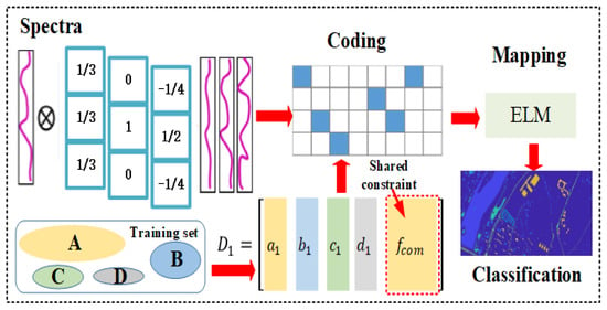
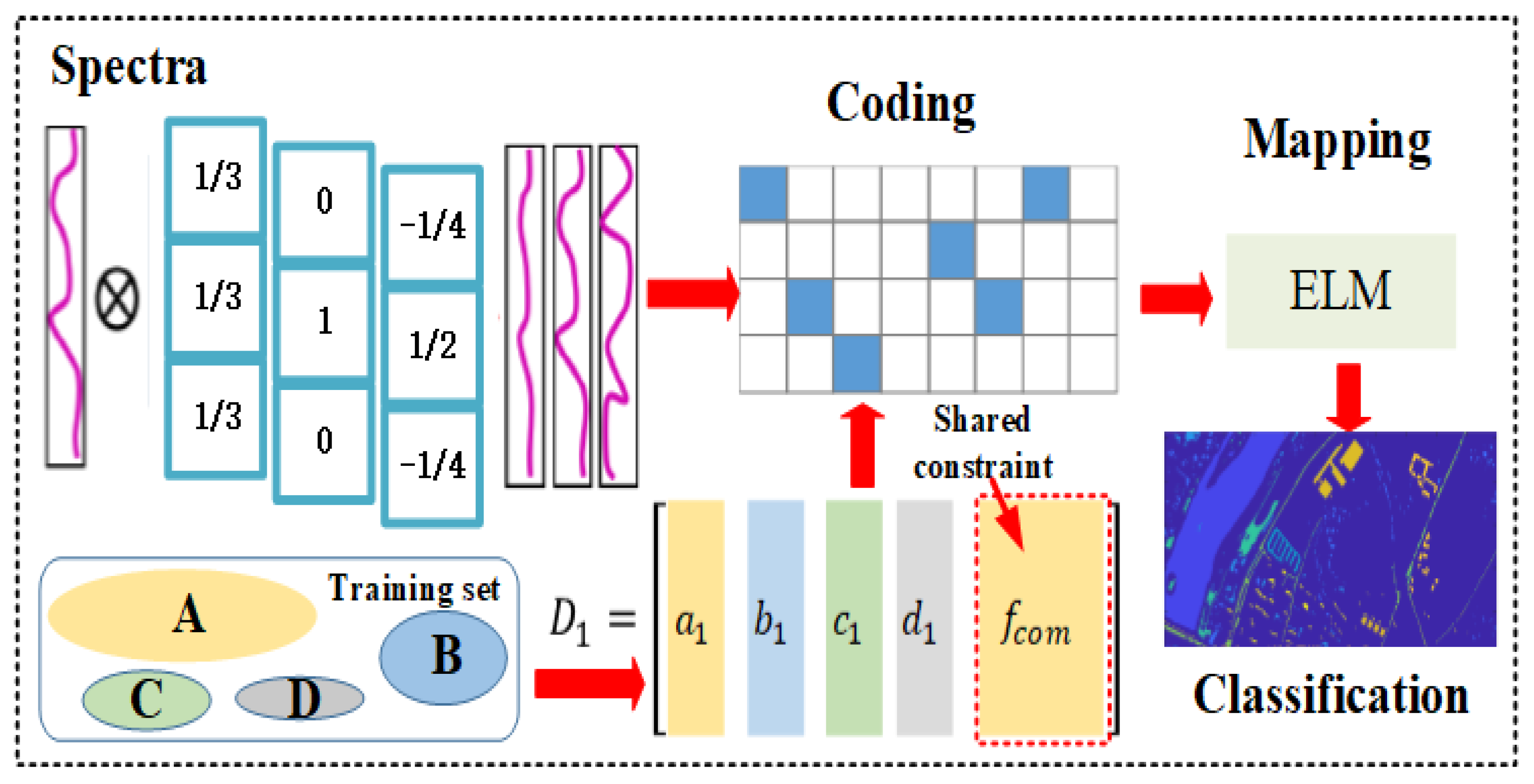
Figure 1 shows the workflow of the proposed framework in which we construct a structured dictionary to extract spectral features for classification application. Spectral convolution is first introduced into our model to extract the abundant information. Following the convolution, the corresponding coding representations are built for the test spectral data. We design the shared constraint for all of subdictionaries to enhance the discriminative ability of the structured dictionary. Finally, the ELM model is adopted to map the coding coefficients to the corresponding labels.

Figure 1. Workflow of the proposed feature extraction model.

2.3.1. Spectral Convolution

The HSI data contain a massive amount of spectral characteristics, such as reflection peaks and valleys, which play important roles in spectral classification. To extract this spectral information, we design different convolution masks for the original samples. The masks are as follows:

$$\left[M_1=\left[\begin{array}{c}0\\ 1\\ 0\end{array}\right],M_2=\left[\begin{array}{c}1/3\\ 1/3\\ 1/3\end{array}\right],M_3=\left[\begin{array}{c}-1/4\\ 1/2\\ -1/4\end{array}\right]\right].$$

(8)

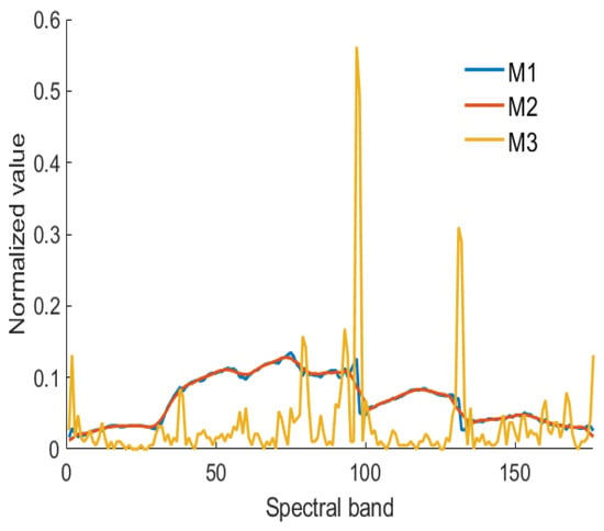
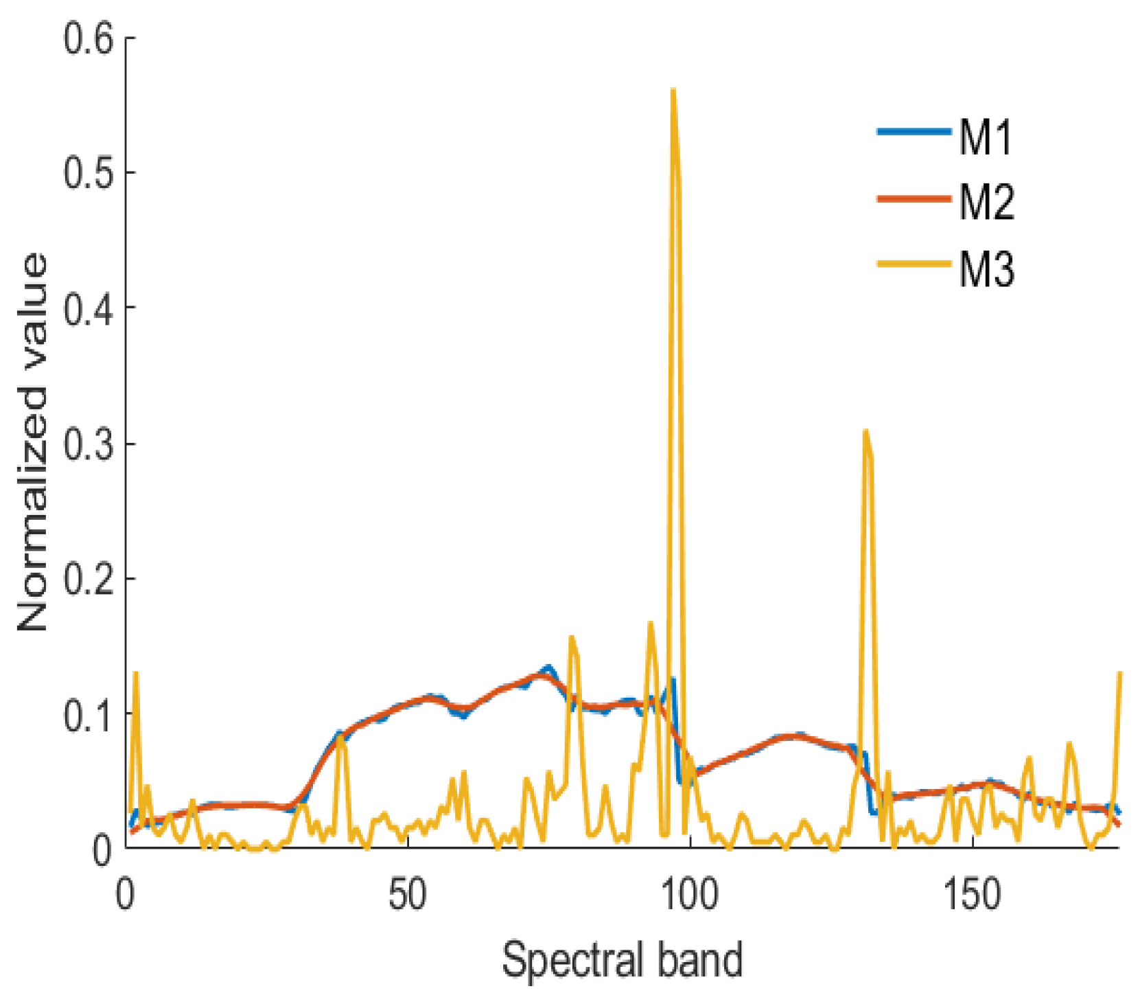
To achieve stable classification performance, we apply $M_1$ to preserve the original data. Inspired by the wave transform, we design mask $M_2$ to extract the main structure (mean values) of spectral samples and mask $M_3$ to capture the detailed information (local variation) of the spectra. As shown in Figure 2, the results of $M_2$ capture the main signal of spectra ($M_1$) and the values of $M_3$ change with the local variation in the spectra ($M_1$). Mask $M_2$ can be adopted to describe the main structure of spectral samples, while mask $M_3$ can be applied to describe the local reflection valleys and peaks of spectral data. However, the running time is closely related to the number of masks. In this work, we only employ three convolutional masks to extract the spectral information, and there are other possible masks that can be applied to extract the spectral characteristics.

Figure 2. Examples of spectral data with different convolution masks.

2.3.2. Structured Dictionary

To encode the spectral information, most of the dictionary-based methods [34,35] are based on the sparsity constraint under the following framework:

$$\underset{D,A}{argmin}{∥X-DA∥}_F^2+\lambda {∥A∥}_p+\phi \left(D_i,A_i\right),$$

(9)

where $\lambda \ge 0$ is a scalar constant. The first term ${\parallel X-DA\parallel }_F^2$ is the fidelity constraint to ensure the representation ability of trained dictionary. The second term ${\parallel A\parallel }_p$ is the sparsity constraint, and the remaining term $\phi \left(D_i,A_i\right)$ is the additional constraint for some discrimination promotion function. These models will train a structured dictionary to represent signals, which will promote discrimination between classes. However, the sparsity constraint is time consuming on the coding coefficients, making the model inefficient. More importantly, the role of sparse coding in classification is still an open problem [36,37,38], and some experts have argued that sparse coding may not be crucial for dictionary classification.

As described in [38], the block-diagonal constraint is an efficient way to calculate coding coefficients. Here, we built the structured dictionary model as follows:

$$\{A,D\}=\underset{A,D}{argmin}\sum _{i=1}^C{∥X_i-D_i{A}_i∥}_F^2+\sum _{j=1,j\ne i}^C{∥A_{ij}∥}_F^2,$$

(10)

where the coefficient matrix A will be nearly block diagonal. The objective function in Equation (10) is generally non-convex. We introduce a variable matrix P to calculate the coefficient matrix A. Matrix $P\in R^{N_A\times L}$ is an encoder, and code A can be calculated as $A=PX$. With the encoder $P=[P_1;\dots ;P_j;\dots ;P_C]$, we want the encoder $P_j$ to be able project the samples $X_i$ ($j\ne i$) to a nearly null space, i.e., $P_j{X}_i\approx 0,\forall j\ne i$. Therefore, Equation (10) can be relaxed to the following problem:

$$\{A,D,P\}=\underset{A,D,P}{argmin}\sum _{i=1}^C{∥X_i-D_i{A}_i∥}_F^2+\tau {∥P_i{X}_i-A_i∥}_F^2+\lambda {∥P_i\overline{X_i}∥}_F^2,$$

(11)

where $\tau$ and $\lambda$ are scalar constants, $P_i{X}_i=A_i$, and $\overline{X_i}$ denotes the complementary data matrix of subset $X_i$ in the whole training set X. Equation (11) can be implemented via a two-stage iterative algorithm: updating A with fixed D and P and updating D and P with fixed A.

(1) Suppose that D and P are fixed, and A are updated as follows:

$$\begin{array}{c}\hfill \left\{A\right\}=\underset{A}{argmin}\sum _{i=1}^C{∥X_i-D_i{A}_i∥}_F^2+\tau {∥P_i{X}_i-A_i∥}_F^2.\end{array}$$

(12)

Equation (12) is a standard least squares problem, and we achieve the closed-form solution:

$$\begin{array}{c}\hfill A_i^{(k+1)}={\left({D_i^{\left(k\right)}}^T{D}_i^{\left(k\right)}+\tau I\right)}^{-1}\left(\tau P_i^{\left(k\right)}{X}_i+{D_i^{\left(k\right)}}^T{D}_i^{\left(k\right)}\right),\end{array}$$

(13)

where I is the unit matrix.

(2) Fixing A, D and P are updated as follows:

$$\left\{\begin{array}{c}\left\{P\right\}={argmin}_P\sum _{i=1}^C\tau {∥P_i{X}_i-A_i∥}_F^2+\lambda {∥P_i\overline{X_i}∥}_F^2\hfill \\ \left\{D\right\}={argmin}_D\sum _{i=1}^C{∥X_i-D_i{A}_i∥}_F^2,s.t.{∥d_i∥}_2^2\le 1\hfill \end{array}\right.,$$

(14)

where $d_i$ is the atom of the structured dictionary and ${∥d_i∥}_2^2\le 1$ is to make the dictionary more stable. The closed-form solution of P can be obtained as:

$$P_i^{k+1}=\tau A_i^{\left(k\right)}{X}_i^T{\left(\tau X_i{X}_i^T+\lambda \overline{X_i}{\overline{X_i}}^T+\gamma I\right)}^{-1},$$

(15)

where $\gamma$ is a small number. D can be calculated by introducing a variable S:

$$\{D,S\}=\underset{D,S}{argmin}\sum _{i=1}^C{∥X_i-D_i{A}_i∥}_F^2\hspace{1em}s.t.\hspace{1em}D=S, {∥d_i∥}_2^2\le 1.$$

(16)

The optimal solution of Equation (16) can be achieved by the alternating direction method of multipliers (ADMM) algorithm [39]:

$$\left\{\begin{array}{c}{D}^{k+1}=\underset{D}{argmin}\sum _{i=1}^C{∥X_i-D_i^{\left(k\right)}{A}_i^{\left(k\right)}∥}_F^2+\rho {∥D_i^{\left(k\right)}-S_i^{\left(k\right)}+T_i^{\left(k\right)}∥}_F^2\hfill \\ S^{k+1}=\underset{S}{argmin}\sum _{i=1}^C\rho {∥D_i^{(k+1)}-S_i^{\left(k\right)}+T_i^{\left(k\right)}∥}_F^2\hfill \\ T^{k+1}=T^k+D^{(k+1)}-S^{(k+1)},\hfill \end{array}\right.$$

(17)

where $\rho$ is an ever-changing value with a fixed ratio and T is a temp matrix. All these closed-form solutions converge rapidly, and a balance between the discrimination and representation power of the model can be achieved.

2.3.3. Shared Constraint

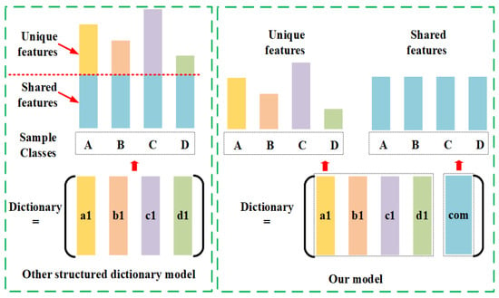
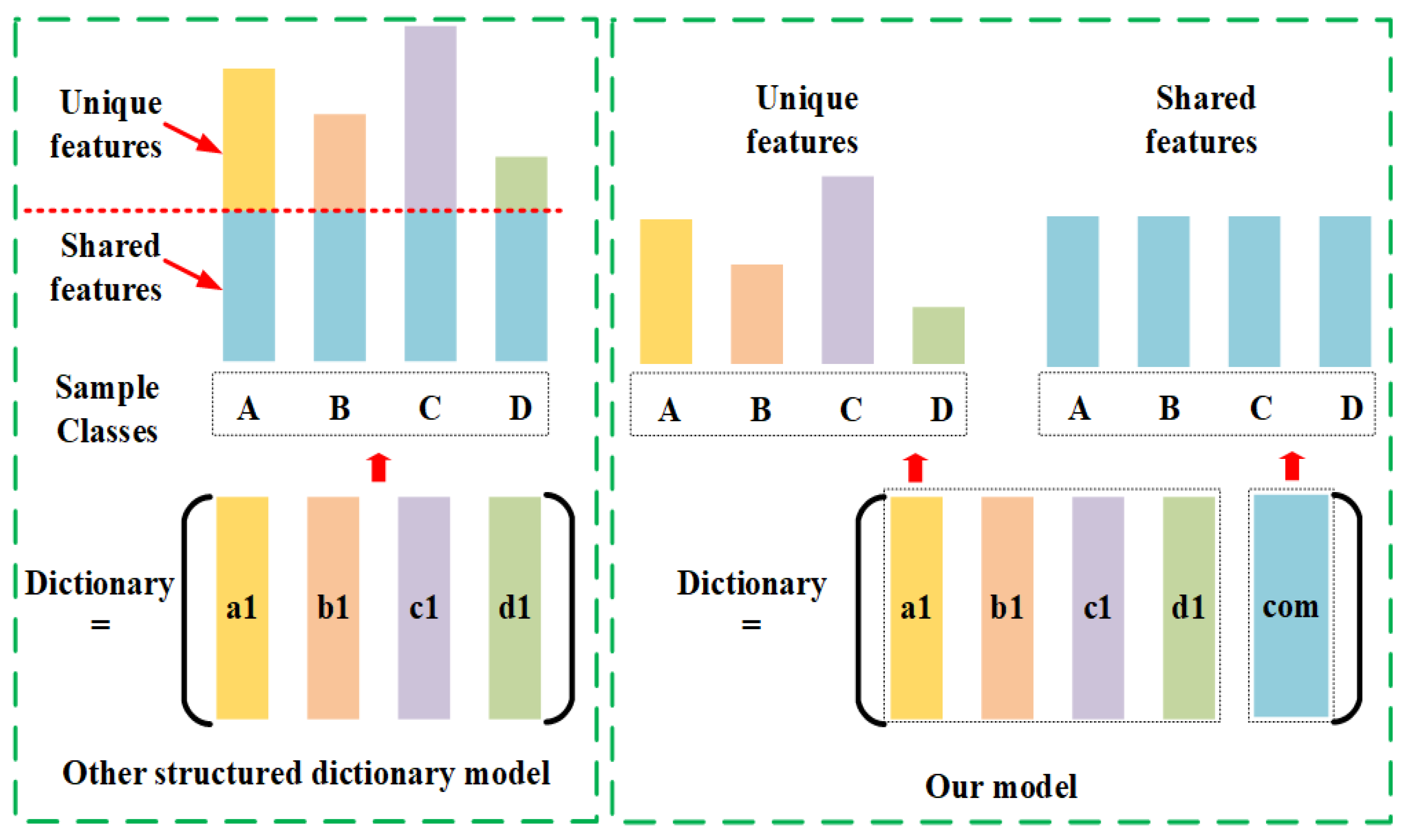
To improve the representation and reconstructive ability of the subdictionaries, we design the shared constraint for subdictionaries. As shown in Figure 3, the test samples contain the shared features, and our shared constraint (the $com$ subdictionary) is added to describe duplicated information (shared features). Then, the discriminative features will be “amplified” relative to the original ones, and constructing a new structured dictionary is easier than ever.

Figure 3. Overview of the built dictionary for different models. Shared constraints are applied for structured dictionaries to represent the shared features between subdictionaries, and unique features can acquire effective expressions.

Here, we design a subdictionary $D_{com}$ to calculate the class-shared characteristics as follows:

$$D=\{D_1,D_2,\dots ,D_C,D_{com}\},$$

(18)

where $D_{com}$ denotes the shared subdictionary. The corresponding objective function is modified as follows:

$$\begin{array}{cc}\hfill \{A,D\}& =\underset{A,D}{argmin}\sum _{i=1}^C{∥X_i-D_i{A}_i∥}_F^2+{∥X_i-D_{com}{A}_{com}∥}_F^2+\sum _{j=1,j\ne i}^C{∥A_{ij}∥}_F^2,\hfill \\ \hfill & =\underset{A,D}{argmin}\sum _{i=1}^C{∥X_i-D_{icom}{A}_{icom}∥}_F^2+\sum _{j=1,j\ne i}^C{∥A_{ij}∥}_F^2,\hfill \end{array}$$

(19)

where $D_{icom}=[D_i,D_{com}]$ and $A_{icom}=[A_i,A_{com}]$. The introduction of $D_{com}$ will not affect the solution procedure. With the calculation of term $\parallel X_i-D_{com}{A}_{com}{\parallel }_F^2$, the results of term ${\sum }_{i=1}^C{\sum }_{j=1,j\ne i}^C{∥A_{ij}∥}_F^2$ tend to be closer to zero, and the corresponding reconstructive ability of the structured dictionary will be improved.

2.3.4. Feature Extraction Framework

We construct the structured dictionary and encode the spectral information of HSIs. The coding coefficients A will be fed into the learning classifier to achieve better performance than directly using the minimum reconstruction error for classification. Different learning classifiers, such as SVM [12] and neural networks (NNs), can be employed to map the coding coefficients. However, these tools are often time consuming. Therefore, we employ an efficient machine technique, i.e., the extreme learning machine, to classify the HSIs.

In [40], Huang et al. proposed an ELM for generalized single-hidden-layer feed-forward neural networks (SLFNs), which has been widely applied in various application [41,42]. The ELM tries to learn an approximation function based on the training data. Suppose that SLFNs with K hidden nodes can be represented as follows:

$$f_L\left({\mathbf{x}}_i\right)=\sum _{j=1}^{K}g({\mathbf{x}}_i,{\mathbf{a}}_{ij},{\mathbf{b}}_{ij}){\beta }_j,$$

(20)

where ${\mathbf{a}}_{ij}$ is the input weight connecting the input ${\mathbf{x}}_i$ to the j-th hidden node, ${\mathbf{b}}_{ij}$ is the bias connecting the input ${\mathbf{x}}_i$ with the j-th hidden node, $g(·)$ is the activation function, and ${\beta }_j$ is the output weight of the j-th hidden node. The activation function $g(·)$ can be any nonlinear piecewise continuous function as follows:

$$g(\mathbf{x};\theta )=\frac{1}{1+exp(-(a^{T}X+b))},$$

(21)

$$g(\mathbf{x};\theta )=exp(-b\parallel X-a{\parallel }_2),$$

(22)

where Equations (21) and (22) are the sigmoid and radial basis function (RBF), $\theta =(a,b)$ are the parameters of the mapping function, and ${\parallel ·\parallel }_2$ denotes the Euclidean norm.

Huang et al. [43] proved that SLFNs can approximate any continuous target function over any compact subset X with the above sigmoid and RBF functions. Training ELMs is equivalent to settling a regularized least-squares problem, which is considerately more efficient than training an SVM or learning with back-propagation. Therefore, in our model, an ELM is adopted for mapping the coding coefficients into different classes of HSIs.

3. Experimental Results and Discussion

In this section, we compare the performance of our proposed method with other feature extracting models, including SVM [12], FDDL [35], DPL [38], ResNet [44], RNN [21], and CNN [21] for HSI classification. We report the overall accuracy (OA), average accuracy (AA), and kappa coefficient of the different datasets and present the corresponding classification maps. The proposed method is evaluated, and relevant results are summarized and discussed in detail as follows.

3.1. Compared Methods and Evaluation Indexes

The SVM model (the codes for SVM were otained from https://www.csie.ntu.edu.tw/~cjlin/libsvm/) is a representative kernel-based method and has shown effective performance in HSI classification [12,13,45]. Yang et al. [35] proposed a complicated model named FDDL (the codes of FDDL were from http://www4.comp.polyu.edu.hk/~cslzhang/papers.htm), which was applied in HSI classification in [46]. The DPL [38] method (http://www4.comp.polyu.edu.hk/~cslzhang/papers.htm) is constructed to reduce the running time of learning the dictionary model. Convolutional neural networks (CNNs) [21] (all the CNNs models were downloaded from https://github.com/BehnoodRasti/HyFTech-Hyperspectral-Shallow-Deep-Feature-Extraction-Toolbox) are the most popularly adopted deep model for hyperspectral classification. Compared to traditional deep fully connected networks, CNNs possess weight-sharing and local-connection characteristics, making their training processes more efficient and effective. ResNet [44] adopts a residual networks to address the degradation problem and enhances the convergence rate of the CNN model, which is employed in HSI classification [47]. Recurrent neural networks (RNNs) [48,49] process all the spectral bands as a sequence and adopt a flexible network structure to classify HSIs. All experiments were repeated 10 times with the average classification results reported for comparison.

We used the following criteria to evaluate the performance of the different methods for HSI classification used in this paper, which include:

Overall accuracy (OA): the number of correctly classified HSI pixels divided by the total number of tests [50];

Average accuracy (AA): the average value of the classification accuracies of all classes [50];

Kappa coefficient: A statistical measurement of agreement between the final classification and the ground-truth map [50].

3.2. Discussions of Different Datasets

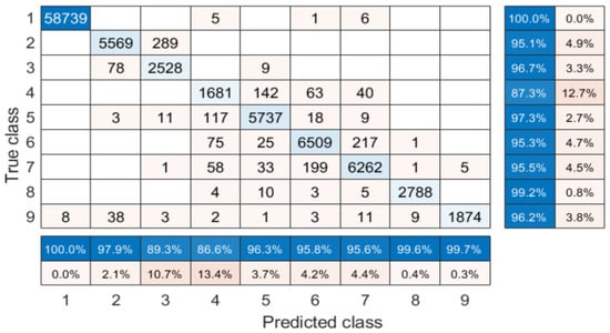
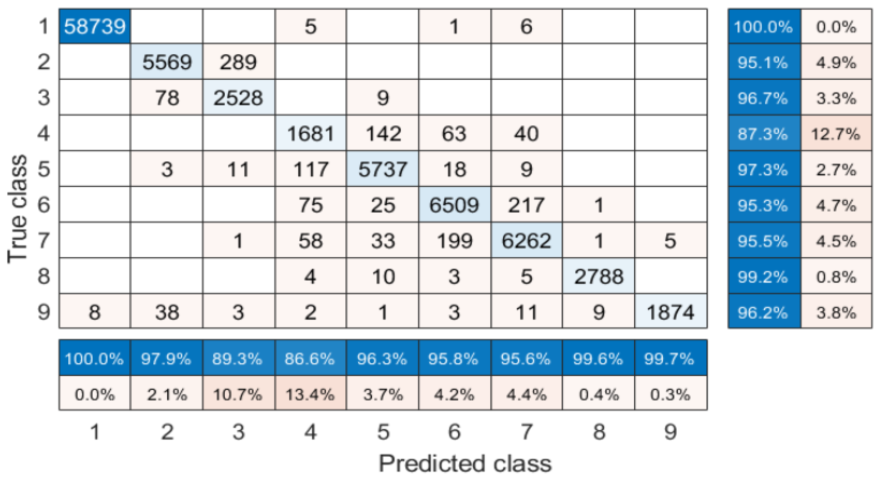
(1) Center of Pavia: Table 4 lists the classification results of the compared algorithms, and Figure 4 shows the confusion matrix of our model (only to one decimal place). In Table 4, one can observe that all the CNN-based models have a good performance. The best performance is achieved by the proposed framework whose OA, AA, and kappa coefficients are $98.39\%$, $95.83\%$, and $97.23\%$, respectively. Compared with the dictionary learning- and deep learning-based models, our model gains significant classification accuracy for this dataset, especially for Class No. 2; see Figure 4. The confusion matrix for our model is shown in Figure 4, indicating that our algorithm distinguishes surface regions quite effectively.

Table 4. Classification accuracy for the Center of Pavia dataset. FDDL, Fisher discriminant dictionary learning.

Class No.	SVM	FDDL	DPL	ResNet	RNN	CNN	Ours
1	0.9866	0.9882	0.9856	0.9845	0.9836	0.9966	0.9998
2	0.6302	0.2319	0.3743	0.6641	0.4118	0.7496	0.9507
3	0.9708	0.9851	0.9682	0.9644	0.9902	0.9669	0.9667
4	0.5055	0.3760	0.2568	0.4877	0.4646	0.5256	0.8728
5	0.9969	0.9848	0.9729	0.9835	0.9924	0.9905	0.9732
6	0.6659	0.6944	0.8576	0.7035	0.8335	0.9331	0.9534
7	0.9163	0.8811	0.9143	0.9363	0.9465	0.9503	0.9547
8	0.9416	0.9595	0.9711	0.9504	0.9794	0.9904	0.9922
9	0.9965	0.9643	0.9825	0.9895	0.9930	0.9874	0.9616
OA	0.9234	0.9057	0.9244	0.9289	0.9331	0.9663	0.9839
AA	0.8456	0.7850	0.8093	0.8515	0.8439	0.8989	0.9583
kappa	0.8927	0.8677	0.8937	0.9004	0.9060	0.9524	0.9723

Figure 4. The confusion matrix of our model on the Pavia of Center dataset.

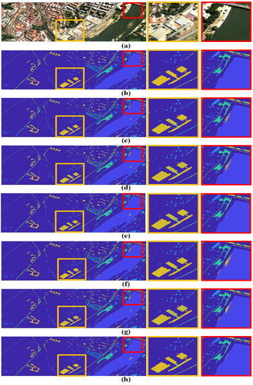
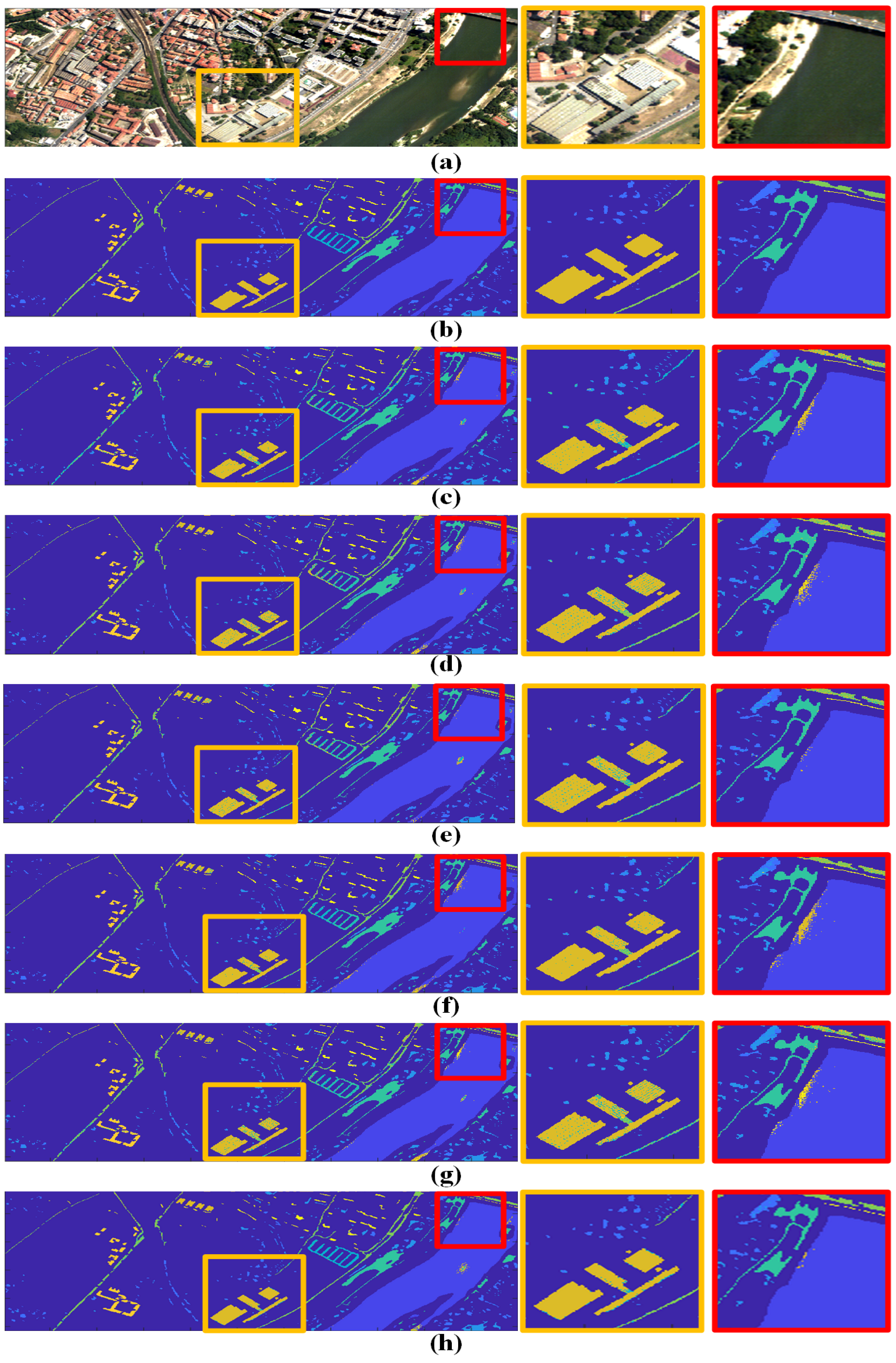
For illustrative purposes, Figure 5 shows the obtained classification maps of the compared methods on the Center of Pavia dataset. Figure 5a,b is the RGB image and ground truth map, and Figure 5c–h is the corresponding classification results of SVM, FDDL, DPL, ResNet, RNN, CNN, and the proposed model. We employ yellow and red rectangles to highlight the interesting regions. We can observe from Figure 5 that the classification maps obtained by the proposed feature extractor are smoother in the regions sharing the same materials and sharper on the edges between different materials. The classification map produced from our model is the closest one compared with the results from other approaches. Our method is capable of extracting the intrinsic invariant feature representation from the HSI, achieving a more effective feature extraction.

Figure 5. Classification maps of the Center of Pavia dataset with the compared methods: (a) RGB image; (b) ground truth; (c) FDDL; (d) DPL; (e) ResNet; (f) RNN; (g) CNN; (h) ours. The yellow and red rectangles correspond to building and water areas.

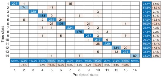
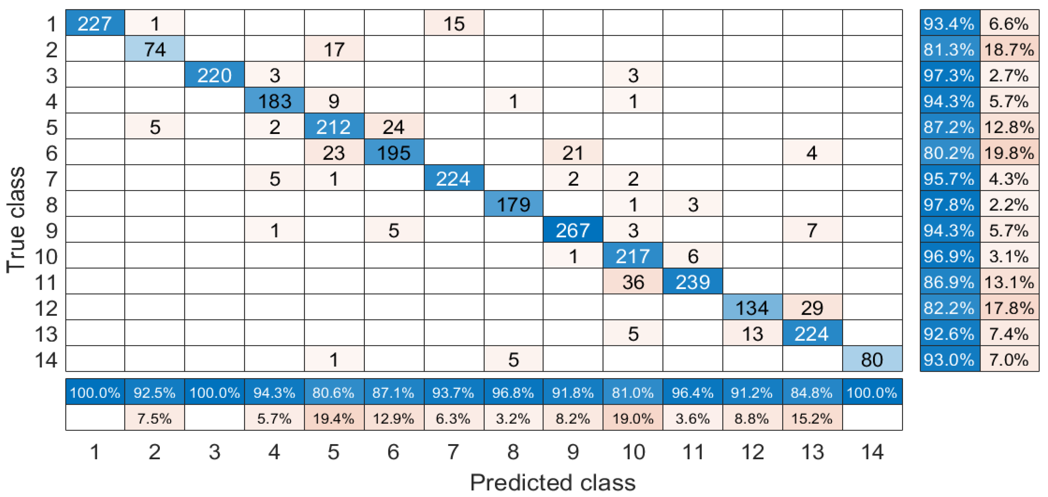
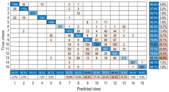
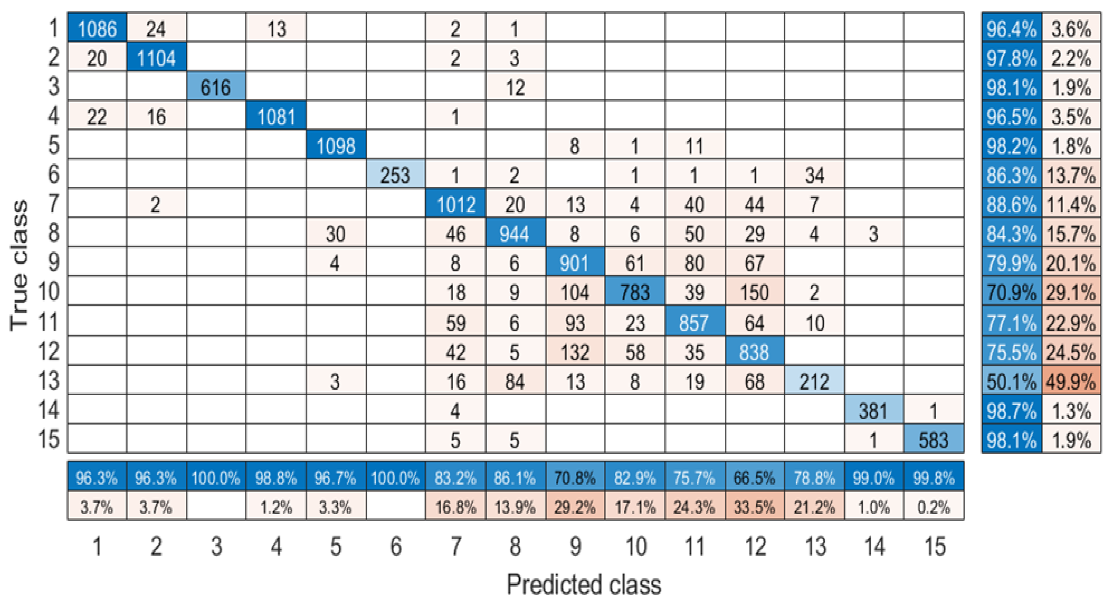
(2) Botswana: The class-specific classification accuracies for the Botswana dataset and corresponding confusion matrix of our model are provided in Table 5 and Figure 6, respectively. From the results, one can see that the proposed algorithm outperforms the other algorithms in terms of OA, AA, and kappa, especially for Class Nos. 10 and 13. The proposed method significantly improves the results with a very high accuracy when tested with the Botswana dataset. From the illustrative results in the confusion matrix map, our model shows more discriminative ability between different classes. The confusion matrix can also confirm the class-specific classification accuracies presented in Table 5.

Table 5. Classification accuracy for the Botswana dataset.

Class No.	SVM	FDDL	DPL	ResNet	RNN	CNN	Ours
1	0.9465	0.9712	0.9794	0.9835	0.9346	0.9492	0.9342
2	1.0000	0.8571	0.9341	0.9890	0.9189	0.8333	0.8132
3	0.8451	0.7920	0.8496	0.8274	0.8366	0.9264	0.9735
4	0.8918	0.7887	0.9175	0.8918	0.7846	0.9323	0.9433
5	0.7037	0.6831	0.7284	0.7572	0.7704	0.8219	0.8724
6	0.6831	0.6461	0.6379	0.6214	0.6250	0.7861	0.8025
7	0.9615	0.7479	0.9316	0.9017	0.9234	0.9607	0.9573
8	0.8852	0.9126	0.9836	0.9781	0.8214	0.9005	0.9781
9	0.7279	0.7032	0.6784	0.7739	0.7651	0.7651	0.9435
10	0.7321	0.4777	0.8348	0.8527	0.7704	0.8071	0.9688
11	0.7418	0.7564	0.8945	0.8836	0.8404	0.8517	0.8691
12	0.9080	0.8037	0.8834	0.9816	0.7746	0.8580	0.8221
13	0.5785	0.7810	0.8554	0.7397	0.7371	0.8966	0.9256
14	0.9070	0.6628	0.7907	0.7907	0.7404	0.8901	0.9302
OA	0.8017	0.7515	0.8420	0.8444	0.8017	0.8676	0.9130
AA	0.8223	0.7560	0.8500	0.8552	0.8031	0.8699	0.9095
kappa	0.7854	0.7311	0.8289	0.8316	0.7850	0.8566	0.9057

Figure 6. The confusion matrix of our model on the Botswana dataset.

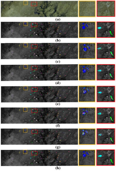
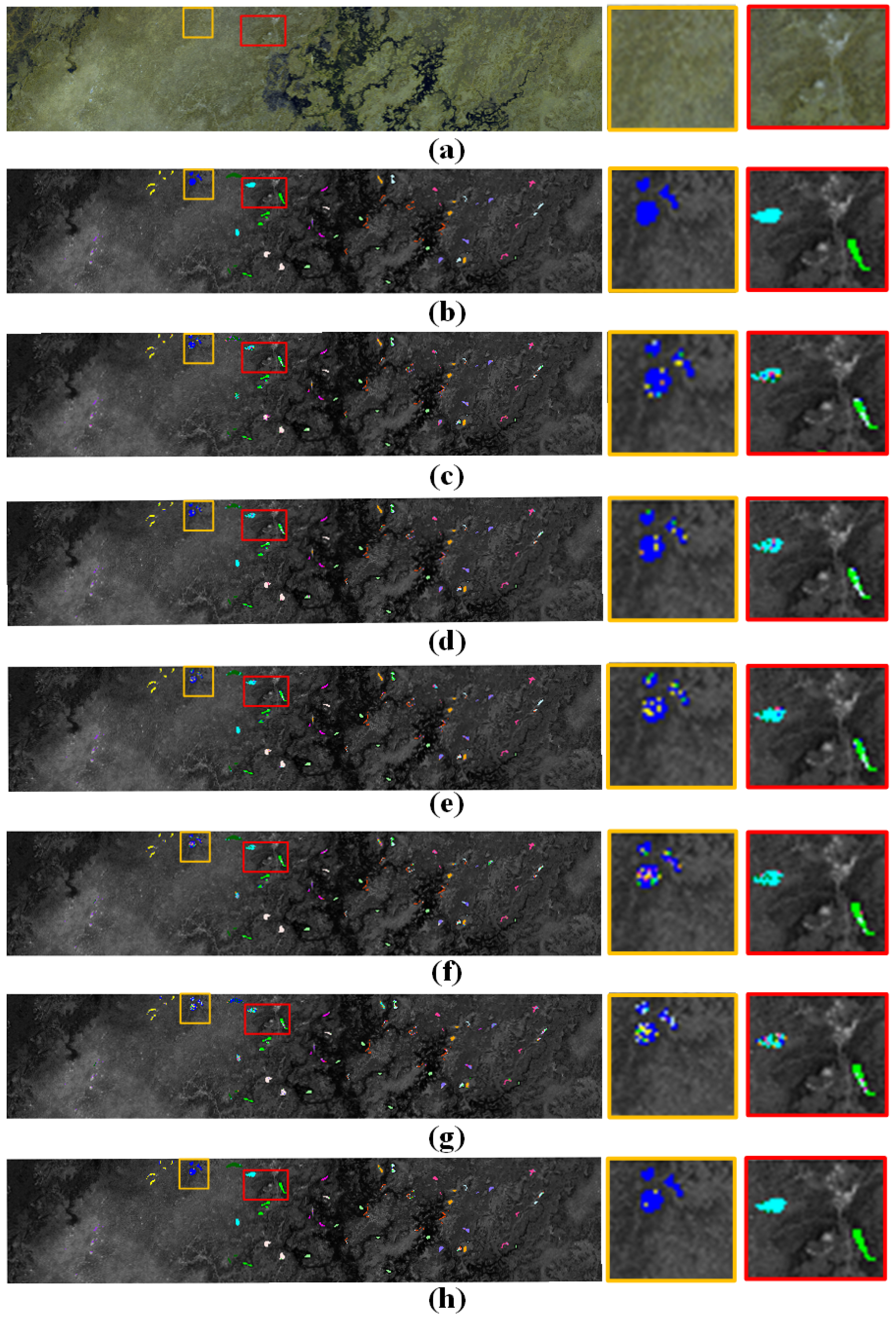
Figure 7 shows the classification maps for the Botswana dataset where Figure 7a,b is the RGB image and ground truth map and Figure 7c–h is the corresponding classification results of SVM, FDDL, DPL, ResNet, RNN, CNN, and the proposed model. We employ yellow and red rectangles to highlight the interesting regions. From the illustrative presentation in the classification maps, the compared algorithms show more noisy scattered point in the maps. The proposed method can remove them and lead to smoother classification results without blurring the boundaries. The result of our model is the closest one compared with the state-of-the-art methods. It demonstrates the effectiveness of the proposed structured dictionary learning model.

Figure 7. Classification maps of the Botswana dataset with the compared methods: (a) RGB image; (b) ground truth; (c) FDDL; (d) DPL; (e) ResNet; (f) RNN; (g) CNN; (h) O = ours. The yellow and red rectangles correspond to grassland and mountain areas.

(3) Houston University 2013: Table 6 lists the classification result of the compared methods on the Houston University 2013 dataset, and Figure 8 shows the corresponding confusion matrix of our model. In Table 6, it is obvious that our model achieves slightly better performance than CNN-based models. The OA, AA, and kappa coefficients of our framework are $86.82\%$, $86.44\%$, and $85.74\%$, respectively. Compared with the dictionary learning- and deep learning-based models, our model gains significant classification accuracy over this dataset, especially for Class Nos. 8, 9, and 12. The confusion matrix for our model is shown in Figure 8, indicating that our algorithm distinguishes surface regions quite effectively.

Table 6. Classification accuracy for the Houston University 2013 dataset.

Class No.	SVM	FDDL	DPL	ResNet	RNN	CNN	Our
1	0.889	0.9076	0.9831	0.9387	0.9538	0.9224	0.9645
2	0.9353	0.9477	0.9814	0.9752	0.9628	0.9824	0.9779
3	0.9586	0.9984	0.9825	0.9904	0.9857	0.9888	0.9809
4	0.8875	0.9446	0.8634	0.9598	0.9714	0.9435	0.9652
5	0.9284	0.9776	0.9902	0.9723	0.9785	0.9663	0.9821
6	0.8703	0.9829	0.9693	0.9590	0.9249	0.9691	0.8635
7	0.6261	0.7881	0.6996	0.7977	0.7820	0.8567	0.8862
8	0.725	0.5188	0.6571	0.5634	0.4223	0.7945	0.8429
9	0.551	0.6557	0.7329	0.7063	0.7045	0.7269	0.7995
10	0.6389	0.4244	0.8462	0.7747	0.7738	0.7808	0.7086
11	0.5117	0.4317	0.5926	0.7752	0.8354	0.7889	0.7707
12	0.5396	0.5315	0.6595	0.6036	0.7450	0.7348	0.7550
13	0.2766	0.5414	0.2884	0.6430	0.5745	0.4879	0.5012
14	0.9689	0.9948	0.9896	0.9896	0.9793	0.9908	0.9870
15	0.9545	0.9882	0.9848	0.9562	0.9781	0.9351	0.9815
OA	0.7409	0.7476	0.8103	0.8255	0.8280	0.8549	0.8682
AA	0.7508	0.7756	0.8147	0.8404	0.8381	0.8579	0.8644
kappa	0.7199	0.7271	0.7949	0.8114	0.8142	0.8431	0.8574

Figure 8. The confusion matrix of our model on the Houston University 2013 dataset.

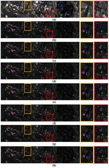
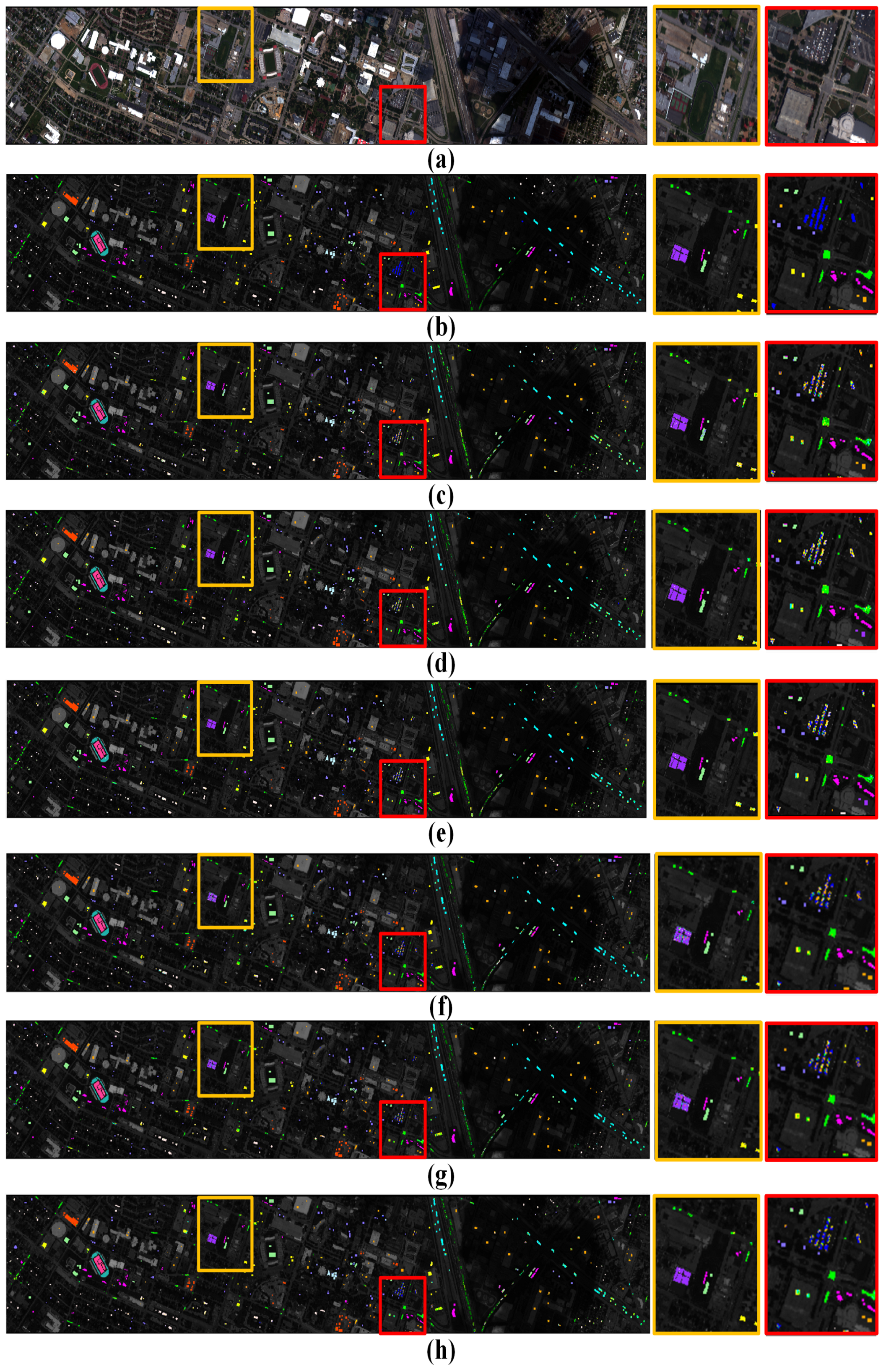
For illustrative purposes, Figure 9 shows the obtained classification maps of the compared methods on the Houston University 2013 dataset. Figure 9a,b is the RGB image and ground truth map, and Figure 9c–h is the corresponding classification results of SVM, FDDL, DPL, ResNet, RNN, CNN, and the proposed model. We employ yellow and red rectangles to highlight the interesting regions. As shown in Figure 9, our model removes the effects of salt-and-pepper noise from the classification maps effectively and simultaneously preserves the meaningful structure or objects. Owing to the robustness in local changes of the spectra, our model obtains more accurate classification maps in the area in and around the parking lot. Generally speaking, our model clearly shows superior performance in effective classification of HSIs.

Figure 9. Classification maps of the Houston University 2013 dataset with the compared methods: (a) RGB image; (b) ground truth; (c) FDDL; (d) DPL; (e) ResNet; (f) RNN; (g) CNN; (h) ours. The yellow and red rectangles correspond to building areas and the parking lot.

3.3. Small Training Samples

The impact of the sample size for HSI classification has been reported in many research studies [23,24,28]. To confirm the effectiveness of our framework on small training samples, we randomly selected $5\%$ of the Botswana dataset for training and the rest for testing. As shown in Table 7, the classification performance is extremely susceptible to the number of training data. The reduction to $5\%$ of the training samples leads to a decrease of about $2\%\sim 4\%$ in classification accuracy. The OA, AA, and kappa of our model are 88.42%, 88.95%, and 87.46%, beating all other compared methods. This result suggests that our model has the potential to achieve higher level accuracy with a limited sample size.

Table 7. The classification results with 5% of the Botswana dataset for training the models.

Class No.	SVM	FDDL	DPL	ResNet	RNN	CNN	Ours
1	0.9689	0.9805	0.8755	1.0000	0.6314	0.9312	1.0000
2	0.9896	0.7917	0.9896	0.9896	0.2370	0.7934	0.9063
3	0.6527	0.6862	0.8745	0.8452	0.7762	0.8779	0.9791
4	0.9122	0.6195	0.9220	0.8439	0.0714	0.8846	0.9073
5	0.5078	0.6094	0.7070	0.7891	0.7619	0.8333	0.8242
6	0.5391	0.5234	0.7070	0.6641	0.4356	0.7194	0.7500
7	0.8178	0.9474	0.7814	0.8866	0.8291	0.9551	0.9393
8	0.9016	0.7824	0.9585	0.9793	0.3591	0.8396	0.9482
9	0.5017	0.5786	0.7893	0.7525	0.6681	0.7523	0.8528
10	0.6017	0.7203	0.9110	0.7712	0.8125	0.7079	0.7839
11	0.8172	0.6276	0.7276	0.8793	0.8671	0.7595	0.9483
12	0.7209	0.5523	0.6047	0.9360	0.4409	0.7661	0.9419
13	0.5647	0.7333	0.9490	0.5765	0.7788	0.8718	0.7490
14	0.8242	0.9231	0.8132	0.8132	0.2222	0.7938	0.9231
OA	0.7125	0.7067	0.8215	0.8250	0.6122	0.8192	0.8842
AA	0.7355	0.7188	0.8293	0.8368	0.5637	0.8204	0.8895
kappa	0.6889	0.6827	0.8067	0.8107	0.5815	0.8042	0.8746

3.4. Time Cost

All the experiments in this paper were implemented with MATLAB 2018b and Python on a Windows 10 operation system and conducted on an Intel Core i7-8700 CPU 3.20 GHz desktop with 16GB memory. The training and testing time of different models are listed in Table 8. Overall, the training and testing time of our model are far less than the SVM- and CNN-based models, which clearly shows the superior efficiency of our approach in classification application.

Table 8. Training and testing time of the HSI classification algorithms on the three datasets.

Dataset	Time (s)	SVM	CNN	RNN	Ours
					Coding	ELM
Pavia of	Training	286.14	404.16	800.68	0.43	1.48
Center	Testing	6.78	8.21	9.33	4.50$\times {10}^{-4}$	0.63
Botswana	Training	51.44	70.03	296.24	0.03	0.05
	Testing	1.77	1.9	3.64	$2.90\times {10}^{-4}$	0.13
Houston	Training	62.50	106.04	256.01	0.15	0.25
University 2013	Testing	2.11	2.66	3.12	$3.20\times {10}^{-5}$	0.17

4. Conclusions

In this work, we propose an efficient spectral feature extraction framework for HSI data. This algorithm is more suitable for low spatial resolution HSIs with a lack of spatial features. To improve the efficiency of our framework, we replace the sparsity constraint with the block-diagonal constraint to reduce the coding computation and employ an ELM model to map the coding coefficients. More importantly, we design spectral convolution and perform the dictionary learning on these features to capture more local spectral characteristics of the data. We also design a new shared constraint to construct a discriminative dictionary in the learning. Extensive experiments are conducted on three HSI datasets, and both qualitative and quantitative results demonstrate the effectiveness of the proposed feature learning model. Furthermore, the proposed approach consistently achieves higher classification accuracy even under a small number of training samples. In comparison to the SVM- and CNN-based models, our framework requires much less computation time, which demonstrates its potential and superiority in the HSI classification task. In the future, we will continue to incorporate the spatial information into the model to further strengthen the feature representation ability.

References

- Dou, P.; Zeng, C. Hyperspectral Image Classification Using Feature Relations Map Learning. Remote Sens. 2020, 12, 2956. [Google Scholar] [CrossRef] [Scilit]
- Santos-Rufo, A.; Mesas-Carrascosa, F.-J.; García-Ferrer, A.; Meroño-Larriva, J.E. Wavelength Selection Method Based on Partial Least Square from Hyperspectral Unmanned Aerial Vehicle Orthomosaic of Irrigated Olive Orchards. Remote Sens. 2020, 12, 3426. [Google Scholar] [CrossRef] [Scilit]
- Li, J.; Huang, X.; Gamba, P.; Bioucas-Dias, J.M.; Zhang, L.; Benediktsson, J.A.; Plaza, A. Multiple Feature Learning for Hyperspectral Image Classification. IEEE Trans. Geosci. Remote Sens. 2015, 53, 1592–1606. [Google Scholar] [CrossRef] [Scilit]
- Yang, S.; Shi, Z. Hyperspectral Image Target Detection Improvement Based on Total Variation. IEEE Trans. Image Process. 2016, 25, 2249–2258. [Google Scholar] [CrossRef] [Scilit] [PubMed]
- Liu, X.; Deng, C.; Chanussot, J.; Hong, D.; Zhao, B. Stfnet: A two-stream convolutional neural network for spatiotemporal image fusion. IEEE Trans. Geosci. Remote Sens. 2019, 57, 6552–6564. [Google Scholar] [CrossRef] [Scilit]
- Landgrebe, D. Hyperspectral image data analysis. IEEE Signal Process. Mag. 2002, 19, 17–28. [Google Scholar] [CrossRef] [Scilit]
- Bayliss, J.; Gualtieri, J.; Cromp, R. Analysing hyperspectral data with independent component analysis. Proc. Int. Soc. Opt. Eng. 1997, 3240, 133–143. [Google Scholar]
- Rodarmel, C.; Shan, J. Principal Component Analysis for Hyperspectral Image Classification. Surv. Land Inf. Syst. 2002, 62, 115–122. [Google Scholar]
- Ji, S.; Ye, J. Generalized linear discriminant analysis: A unified framework and efficient model selection. IEEE Trans. Neural Netw. 2008, 19, 1768–1782. [Google Scholar]
- Scholkopf, B.; Smola, A. Learning with Kernels? Support Vector Machines, Regularization, Optimization and Beyond; MIT Press: Cambridge, MA, USA, 2002; pp. 1768–1782. [Google Scholar]
- Camps-Valls, G.; Bruzzone, L. Kernel-based methods for hyperspectral image classification. IEEE Trans. Geosci. Remote Sens. 2005, 43, 1351–1362. [Google Scholar] [CrossRef] [Scilit]
- Archibald, R.; Fann, G. Feature selection and classification of hyperspectral images with support vector machines. IEEE Geosci. Remote Sens. Lett. 2007, 4, 674–677. [Google Scholar] [CrossRef] [Scilit]
- Bahria, S.; Essoussi, N.; Limam, M. Hyperspectral data classification using geostatistics and support vector machines. Remote Sens. Lett. 2011, 2, 99–106. [Google Scholar] [CrossRef] [Scilit]
- Bruzzone, L.; Chi, M.; Marconcini, M. A novel transductive svm for semisupervised classification of remote-sensing images. IEEE Trans. Geosci. Remote Sens. 2006, 44, 3363–3373. [Google Scholar] [CrossRef] [Scilit]
- Chen, Y.; Lin, Z.; Zhao, X.; Wang, G.; Gu, Y. Deep learning-based classification of hyperspectral data. IEEE J. Sel. Top. Appl. Earth Obs. 2014, 7, 2094–2107. [Google Scholar] [CrossRef] [Scilit]
- Chen, Y.; Zhao, X.; Jia, X. Spectralcspatial classification of hyperspectral data based on deep belief network. IEEE J. Sel. Top. Appl. Earth Obs. 2015, 8, 2381–2392. [Google Scholar] [CrossRef] [Scilit]
- Romero, A.; Gatta, C.; Camps-Valls, G. Unsupervised deep feature extraction for remote sensing image classification. IEEE Trans. Geosci. Remote Sens. 2016, 54, 1349–1362. [Google Scholar] [CrossRef] [Scilit]
- Zhao, W.; Du, S. Spectral-spatial feature extraction for hyperspectral image classification: A dimension reduction and deep learning approach. IEEE Trans. Geosci. Remote Sens. 2016, 54, 4544–4554. [Google Scholar] [CrossRef] [Scilit]
- Chen, Y.; Jiang, H.; Li, C.; Jia, X.; Ghamisi, P. Deep feature extraction and classification of hyperspectral images based on convolutional neural networks. IEEE Trans. Geosci. Remote Sens. 2016, 54, 6232–6251. [Google Scholar] [CrossRef] [Scilit]
- Li, W.; Wu, G.; Zhang, F.; Du, Q. Hyperspectral image classification using deep pixel-pair features. IEEE Trans. Geosci. Remote Sens. 2017, 55, 844–853. [Google Scholar] [CrossRef] [Scilit]
- Rasti, B.; Hong, D.; Hang, R.; Ghamisi, P.; Kang, X.; Chanussot, J.; Benediktsson, J.A. Feature Extraction for Hyperspectral Imagery: The Evolution from Shallow to Deep (Overview and Toolbox). arXiv 2020, arXiv:2003.02822. [Google Scholar] [CrossRef] [Scilit]
- Wright, J.; Yang, A.; Ganesh, A.; Sastry, S.; Ma, Y. Robust face recognition via sparse representation. IEEE Trans. Pattern Anal. Mach. Intell. 2009, 31, 210–227. [Google Scholar] [CrossRef] [Scilit] [PubMed]
- Chen, Y.; Nasrabadi, N.; Tran, T. Hyperspectral image classification using dictionary-based sparse representation. IEEE Trans. Geosci. Remote Sens. 2011, 49, 3973–3985. [Google Scholar] [CrossRef] [Scilit]
- Chen, Y.; Nasrabadi, N.; Tran, T. Hyperspectral image classification via kernel sparse representation. IEEE Trans. Geosci. Remote Sens. 2013, 51, 217–231. [Google Scholar] [CrossRef] [Scilit]
- Gao, S.; Tsang, I.; Chia, L. Sparse representation with kernels. IEEE Trans. Image Process. 2013, 22, 423–434. [Google Scholar]
- Li, C.; Ma, Y.; Mei, X.; Liu, C.; Ma, J. Hyperspectral image classification with robust sparse representation. IEEE Geosci. Remote Sens. Lett. 2016, 13, 641–645. [Google Scholar] [CrossRef] [Scilit]
- Zhang, Q.; Li, B. Discriminative k-svd for dictionary learning in face recognition. In Proceedings of the 2010 IEEE Computer Society Conference on Computer Vision and Pattern Recognition, San Francisco, CA, USA, 13–18 June 2010; pp. 2691–2698. [Google Scholar]
- Du, P.; Xue, Z.; Li, J.; Plaza, A. Learning discriminative sparse representations for hyperspectral image classification. IEEE J. Sel. Top. Signal Process. 2015, 9, 1089–1104. [Google Scholar] [CrossRef] [Scilit]
- Wang, Z.; Nasrabadi, N.; Huang, T. Spatial-spectral classification of hyperspectral images using discriminative dictionary designed by learning vector quantization. IEEE Trans. Geosci. Remote Sens. 2014, 52, 4808–4822. [Google Scholar] [CrossRef] [Scilit]
- Gao, L.; Yu, H.; Zhang, B.; Li, Q. Locality-preserving sparse representation-based classification in hyperspectral imagery. J. Appl. Remote Sens. 2016, 10, 1–15. [Google Scholar] [CrossRef] [Scilit]
- Mei, X.; Pan, E.; Ma, Y.; Dai, X.; Huang, J.; Fan, F.; Du, Q.; Zheng, H.; Ma, J. Spectral-Spatial Attention Networks for Hyperspectral Image Classification. Remote Sens. 2019, 11, 963. [Google Scholar] [CrossRef] [Scilit]
- Yang, X.; Zhang, X.; Ye, Y.; Lau, R.; Lu, S.; Li, X.; Huang, X. Synergistic 2D/3D Convolutional Neural Network for Hyperspectral Image Classification. Remote Sens. 2020, 12, 2033. [Google Scholar] [CrossRef] [Scilit]
- Shu, K.; Wang, D. A Brief Summary of Dictionary Learning Based Approach for Classification. arXiv 2012, arXiv:1205.6544. [Google Scholar]
- Yang, M.; Zhang, L.; Yang, J.; Zhang, D. Metaface learning for sparse representation based face recognition. In Proceedings of the 2010 IEEE International Conference on Image Processing, Hong Kong, China, 26–29 September 2010. [Google Scholar]
- Yang, M.; Zhang, L.; Feng, X.; Zhang, D. Fisher discrimination dictionary learning for sparse representation. In Proceedings of the 2011 International Conference on Computer Vision, Barcelona, Spain, 6–13 November 2011. [Google Scholar]
- Coates, A.; Ng, A. The importance of encoding versus training with sparse coding and vector quantization. In Proceedings of the International Conference on Machine Learning, Bellevue, WA, USA, 28 June–2 July 2011. [Google Scholar]
- Zhang, L.; Yang, M.; Feng, X. Sparse representation or collaborative representation: Which helps face recognition? In Proceedings of the 2011 International Conference on Computer Vision, Barcelona, Spain, 6–13 November 2011. [Google Scholar]
- Gu, S.; Zhang, L.; Zuo, W.; Feng, X. Projective Dictionary Pair Learning for Pattern Classification. Adv. Neural Inf. Process. Syst. 2014, 27, 793–801. [Google Scholar]
- Boyd, S.; Parikh, N.; Chu, E. Distributed Optimization and Statistical Learning via the Alternating Direction Method of Multipliers. Found. Trends Mach. Learn. 2010, 3, 1–122. [Google Scholar] [CrossRef] [Scilit]
- Huang, G.; Zhu, Q.; Siew, C. Extreme learning machine: Theory and applications. Neurocomputing 2006, 70, 489–501. [Google Scholar] [CrossRef] [Scilit]
- Liu, X.; Deng, C.; Wang, S.; Huang, G.; Zhao, B.; Lauren, P. Fast and Accurate Spatiotemporal Fusion Based Upon Extreme Learning Machine. IEEE Geosci. Remote Sens. Lett. 2016, 13, 2039–2043. [Google Scholar] [CrossRef] [Scilit]
- Zhou, S.; Deng, C.; Wang, W.; Huang, G.; Zhao, B. GenELM: Generative Extreme Learning Machine feature representation. Neurocomputing 2019, 362, 41–50. [Google Scholar] [CrossRef] [Scilit]
- Huang, G.; Chen, L.; Siew, C. Universal Approximation Using Incremental Constructive Feedforward Networks With Random Hidden Nodes. IEEE Trans. Neural Netw. 2006, 17, 879–892. [Google Scholar] [CrossRef] [Scilit]
- Zhong, Z.; Li, J.; Ma, L.; Jiang, H.; Zhao, H. Deep residual networks for hyperspectral image classification. In Proceedings of the 2017 IEEE International Geoscience and Remote Sensing Symposium (IGARSS), Fort Worth, TX, USA, 23–28 July 2017; Volume 142–149, pp. 1824–1827. [Google Scholar]
- Zhao, C.; Liu, W.; Xu, Y.; Wen, J. A spectral-spatial SVM-based multi-layer learning algorithm for hyperspectral image classification. Remote Sens. Lett. 2018, 9, 218–227. [Google Scholar] [CrossRef] [Scilit]
- Yuan, Z.; Sun, H.; Ji, K.; Zhou, H. Hyperspectral Image Classification Using Fisher Dictionary Learning based Sparse Representation. Remote Sens. Technol. Appl. 2014, 29, 646–652. [Google Scholar]
- Meng, Z.; Li, L.; Tang, X.; Feng, Z.; Jiao, L.; Liang, M. Multipath Residual Network for Spectral-Spatial Hyperspectral Image Classification. Remote Sens. 2019, 11, 1896. [Google Scholar] [CrossRef] [Scilit]
- Shi, C.; Pun, C. Multi-scale hierarchical recurrent neural networks for hyperspectral image classification. Neurocomputing 2018, 294, 82–93. [Google Scholar] [CrossRef] [Scilit]
- Hang, R.; Liu, Q.; Hong, D.; Ghamisi, P. Cascaded recurrent neural networks for hyperspectral image classification. IEEE Trans. Geosci. Remote Sens. 2019, 57, 5384–5394. [Google Scholar] [CrossRef] [Scilit]
- Mou, L.; Ghamisi, P.; Zhu, X. Deep Recurrent Neural Networks for Hyperspectral Image Classification. IEEE Trans. Geosci. Remote Sens. 2017, 55, 3639–3655. [Google Scholar] [CrossRef] [Scilit]
Publisher’s Note: MDPI stays neutral with regard to jurisdictional claims in published maps and institutional affiliations. |
© 2020 by the authors. Licensee MDPI, Basel, Switzerland. This article is an open access article distributed under the terms and conditions of the Creative Commons Attribution (CC BY) license (http://creativecommons.org/licenses/by/4.0/).