Nexus Biofuel Consumption, Economic Growth and Environment in Saudi Arabia: Current and Prospective

Abstract

Environmental and climatic alterations, coupled with increasing economic activity and increasing energy demand, have reinforced the global need to develop substitute fuels as a means of reducing reliance on fossil fuels. Saudi Arabia has shown increasing biofuel consumption (charcoal and fuelwood) in recent years. Thus, this study was designed to examine the relationship between biofuel energy consfumption, economic growth and the environment. Accordingly, the study comprises dual portions: the first tests the cointegration association among biofuel consumption and economic growth, while the second discovers a cointegration association among biofuel consumption and carbon dioxide emissions. The study also includes a forecasting analysis. Data on biofuel energy consumption, economic growth and the environment were compiled from numerous sources covering the period from 1990 to 2023. Engel–Granger method assessments revealed long-term relationships between bioenergy consumption, economic growth, and environmental quality. FMOLS and DOLS estimates yielded results well-matched with those acquired using the Engel–Granger method. Furthermore, the gross rates of biofuel consumption equal 2.40% for the period 2010–2023 and 2.80% for the forecast period 2023–2035. Similarly, the growth rates of gross domestic product were calculated at 7.50% for the period 2010–2023 and 11.00% for the projected period 2023–2035. Also, the gross rates of CO₂ emissions were calculated at 1.90% for the period 2010–2023 and 0.95% for the projected period 2023–2035. The results indicate that biofuel consumption is expected to continue growing at a faster rate, joined by strong economic growth. Particularly, the projected slowdown in carbon dioxide emissions suggests a possible decoupling of economic activity from environmental degradation. These findings underscore the need to promote biofuel development and clean energy policies to reinforce sustainable economic growth while reducing emissions in the long term.

1. Introduction

Environmental and climatic shifts, combined with expanding economies and rising energy demand, have driven a growing focus on developing alternative fuels to reduce dependence on fossil energy sources [1]. Fossil fuels are a non-renewable source of energy, and their use is a major driver of worldwide warming because of the emission of carbon dioxide [2]. When biofuels are produced sustainably and castoff efficiently, they provide a low-carbon substitute to traditional fossil fuel consumption [3,4]. Biofuels are a vital component of sustainable energy systems, promoting access to ecologically friendly energy bases and supporting overall environmental excellence [5].

Two of the Sustainable Development Goals (SDGs) adopted by the United Nations are directly related to climate change and alleviation strategies: confirming access to reasonable, sustainable, reliable, and contemporary energy for all (SDG 7) and promoting climate action (SDG 13) [6,7]. In line with these worldwide main concerns, Saudi Arabia’s Vision 2030 outlines a motivated renewable energy strategy, establishing the growth of clean energy as a cornerstone of realizing national sustainable development [8,9]. Saudi authorities, led by the National Center for Vegetation Development and Combating Desertification, enforce strict regulations aimed at preserving natural vegetation cover and curbing illegal logging and local charcoal production [10]. Saudi Arabia is one of the leading consumers of charcoal in the Gulf region, accounting for a significant share of regional demand [11]. Globally, the Saudi market represented approximately 8.32% of international charcoal sales in 2024 [12]. Saudi Arabia depends mainly on imported biofuel (charcoal and fuelwood) from the world market [12].

The link between economic growth, energy consumption, and environmental degradation has prompted increasing concern in environmental economics, mainly within the outline of the environmental Kuznets curve and the energy-driven growth hypothesis. These two theoretical approaches offer a broad foundation for understanding the active connections between economic growth, energy consumption and conservational sustainability. Recent empirical studies continue to validate this theoretical proposition across different regions and methodologies [13,14,15,16,17,18].

In relation to Saudi Arabia, the relationship between economic growth, energy consumption and environmental degradation is of specific significance given the Kingdom’s substantial dependence on fossil fuels and its continuing economic conversion in Vision 2030. The latest observational studies deliver robust confirmation supporting the relationship between the environmental Kuznets curve and the energy-driven growth hypothesis in the Saudi economy [19,20,21,22].

Various writers have considered the relation between biofuel consumption and other sectors. They propose a modest influence by studying the dynamics of carbon emission distribution, bioenergy consumption, and economic growth, taking into account non-parametric density methods and quantum regression [23]. Estimates confirm that economic growth and non-renewable energy consumption have a positive impact on carbon emissions, leading to environmental degradation. Conversely, bioenergy consumption displays a significant negative impact on carbon emissions, effectively enhancing environmental sustainability.

A previous study intended to disclose the long-run relation between economic growth, renewable energy consumption, non-renewable energy consumption, globalization and carbon dioxide emissions covering a period from 1970 to 2018. It used an Autoregressive Distributed Lag model as the model for analysis. The study recognized long-term links among such series. The findings indicate that renewable energy use and globalization contribute to emissions reductions, whereas the consumption of non-renewable energy leads to expanded emissions in the long and short term [24].

Refs. [25,26] planned to test the influence of renewable energy consumption on carbon dioxide emissions in the United States during the period 2000–2007, applying a spatially dynamic panel data model. The outcomes designate that the use of renewable energy has a statistically significant negative influence on carbon dioxide emissions, while the association among economic freedom and releases takes a U-shape. Furthermore, the study recognized a statistically significant positive spatial lag for carbon dioxide emissions, signifying a positive correlation between a country’s emissions and those of its neighboring countries.

Other studies were designed to test the influence of hydroelectric and renewable energy consumption on the environmental footprint in G20 nations for the period from 2002 to 2022. The half-panel jackknife causality method and regression method were applied as methods of analysis. The results show that fighting exploitation and renewable energy decrease contamination, while hydroelectric power raises environmental contamination [27,28].

Another study investigated the influence of renewable energy consumption and gross domestic product on carbon dioxide emissions in Thailand, using an Autoregressive Distributed Lag (ARDL) model as an analytical framework [29]. Covering the period from 1980 to 2018, the researchers found that renewable energy consumption had a statistically significant negative effect on short-term carbon dioxide emissions. In contrast, both the lessening of non-renewable energy resources and GDP growth showed statistically significant positive impacts on short- and long-term carbon dioxide emissions.

An additional study was directed to test the influence of renewable energy consumption on per capita carbon dioxide emissions in China during the period 1990–2020 [30], using an ARDL model. The results showed that a one percent rise in per capita renewable energy consumption decreases per capita carbon dioxide emissions by 0.259% in the long term. However, the results also discovered that the fast growth of the renewable energy sector in China is currently leading to increased carbon dioxide emissions, and that a one percent rise in renewable energy intake raises carbon dioxide emissions by between 0.285% and 0.288% in the short term.

Another previous study investigated the role of renewable energy in promoting economic transformation and sustainability [31]. Including journal texts, a literature review was conducted by the Scopus database, concentrating on reviews, book chapters and peer-reviewed articles issued between 2014 and 2023. The examine strategy relied on keywords such as “renewable energy,” “development,” “economics,” and “sustainable development,” filtered by subject, language, document type and geographic scope. The review indicates that the adoption of renewable energy significantly contributes to environmental sustainability by reducing the ecological footprint and lowering greenhouse gas emissions. Among the various renewable energy sources, wind power stands out as an effective driver of sustainable economic development. The findings also highlight the contribution of renewable energy intake in boosting tourism and contributing to gross domestic product growth.

Scientists are discovering alternate fuel types other than traditional ones to lessen carbon emissions through decreasing reliance on fossil fuels [32]. The transport sector is a main user of fuel, making it a critical zone for the adoption of substitute fuels. Their investigation outlined potential conversion scenarios in the transport sector to substitute gasoline and diesel in fossil fuel-dependent economies, comprising Saudi Arabia. It highlighted the potential of substitute fuels, such as ethanol and hydrogen, to meet demands thanks to technological advancements that raise efficacy and decrease costs. The results suggest that by 2050, artificial fuel creation will greatly contribute to reducing crude oil consumption and carbon dioxide emissions. This study, the first of its kind in the region, assessed the application of synthetic fuels made from fossil fuels. The study demonstrates the need for fundamental changes to policies and their implementation mechanisms, and that substitute fuels could become cost-competitive with conventional fuels if Saudi Arabia’s high goals for reducing carbon dioxide emissions are met. The study offers an initial valuation of the execution of the arrangement and emphasizes the necessity for strong rules to accelerate the conversion to substitute fuels.

Another study aimed to examine the impacts of the agriculture, economic growth and renewable energy nexus on carbon dioxide (CO₂) emissions [33]. The main findings include the existence of a long-term association among the elected variables: agriculture pointedly raises CO₂ emissions (in the developing economies of the G20), and renewable energy intake decreases CO₂ emissions (in the developed economies of the G20).

Another study explores the long-term association among renewable energy use, economic growth, and environmental sustainability in Saudi Arabia from 1990 to 2023, using the ARDL model. The results confirm the presence of cointegration, reflecting the dynamic interaction between renewable energy, economic growth, and environmental sustainability [34].

Making reference to previous studies, the significance of this study emerges from its focus on the consumption of charcoal and fuelwood as biofuel, which are less researched in spite of the fact that their consumption is increasing [35]. In addition, this study enriches the literature through the nature of biofuel consumption, which is imported not produced internally. Moreover, this study used different analytical tools: a Granger causality test with its robustness, regression analysis and a forecasting test. Also, the design of this study lies in its objectives; it was planned to evaluate the impact of bioenergy consumption on the economy and the environment. Therefore, the study consists of two portions: the first examines the cointegration relationship between biofuel consumption and GDP, while the second determines the cointegration association among biofuel consumption and carbon dioxide emissions. Moreover, it includes a forecasting analysis for the variables under study.

The following are the research questions and hypotheses:

Research Questions:

Grounded in the Environmental Kuznets Curve and Energy-Led Growth, research questions are derived as follows:

Is there a long-run relationship between biofuel consumption and economic growth?

Is there a long-run relationship between biofuel consumption and CO₂ emission?

Testable Hypotheses:

There is a long-run relationship between biofuel consumption and economic growth.

There is a long-run relationship between biofuel consumption and CO₂ emission

The study is structured as follows: Section 1 provides the introduction, explaining the importance of biofuel energy and highlighting various studies related to this study’s subject. The Section 2 deals with the research methods. The Section 3 comprises the results. The Section 4 offers thediscussion.

2. Materials and Methods

2.1. Data Explanation

The study aimed to test the influence of biofuel consumption on economic growth and environment in Saudi Arabia. Biofuel is represented by charcoal and fuelwood in Terajoule (TJ). The data of such variables were collected from various sources [35,36,37]. It covers the period from 1990 to 2023. The data analysis was performed using the EVIEWS 9 software package, and an overview of the dataset is shown in Table 1.

Table 1. Variables illustration.

Variable	Unit	Sources
Biofuel consumption (E)	Terajoule (TJ)	https://www.fao.org/faostat/ar/#data/BE accessed on 5 February 2026 [35]
Gross domestic product (G)	Billion Dollar (B$)	https://countryeconomy.com/gdp/saudi-arabia accessed on 5 February 2026 [36]
CO2 emissions (C)	Kilotonnes (kt)	https://countryeconomy.com/energy-and-environment/co2-emissions/saudi-arabia accessed on 5 February 2026 [37]

2.2. The Methodology

2.2.1. Descriptive and Graphic Analysis

Descriptive analysis was conducted to summarize the key statistical features of the time series variables, revealing underlying trends, variance patterns, and potential anomalies. This initial assessment provides crucial insights that contribute to econometric modeling and subsequent stability tests [38].

The series’ overall index curves were plotted to provide an initial indication of potential long-term stable relationships between the variables. This graphical approach is a fundamental preliminary technique for the subsequent application of cointegration testing.

2.2.2. Test Long-Run Relationship: (Cointegration Tests)

1. Unit root test: [39,40] determined the subsequent calculation to assess the order of the time series, applying the Dickey–Fuller (ADF) test:

$$∆X_t=C_{t1}+B_1{X}_{t-1}+E_{t1}$$

(1)

$$∆X_t=C_{t2}+b_t+B_2{X}_{t-1}+E_{t2}.$$

(2)

Here, B₁ and B₂ represent the Dickey–Fuller (ADF) test statistics to be estimated. b, C, E and t represent the trend component, constant term, error term, and time index, respectively. The null hypothesis (H₀) states that the variable X has a unit root, while the alternative hypothesis (H₁) assumes that the variable X is stationary. The chain is considered stationary when the t-statistic associated with the Dickey–Fuller (ADF) test coefficient exceeds the corresponding critical value. To inference the results of the ADF test, the Phillips–Perron test (PP) was used [41,42,43].

2. Engle–Granger test: To apply the Engle–Granger cointegration technique, the order of integration of the variables must first be determined, ensuring that all chains are integrated of the same order, usually order 1(1). Once this condition is met, the Engle–Granger test can be applied [41,44]. The technique consists of the following steps:

1. The first regression equation is:

$$X_t=a_{1 }+b_{11 }{Y}_t+z_{t1}$$

(3)

$$Y_t=a_{2 }+b_{12}{X}_t+z_{t2}$$

(4)

where b₁₁ and b₁₂ represent the estimated slope coefficients (Equations (3) and (4)), respectively [45].

2. Then, the Dickey–Fuller (ADF) test is executed to the residuals (z_t1 and z_t2) to determine whether the series of residuals is stationary. If the ADF statistic extracted from the second-stage regression is negative and bigger than the corresponding critical value at the I(1) level, this indicates the coefficients b₅ and b₆ are statistically significant (b₅ and b₆ ≠ 0), and therefore the two series are cointegrated.

To check the robustness of the Engle–Granger test results, alternative cointegration methods (dynamic ordinary least squares (DOLS) and fully modified ordinary least squares (FMOLS) models) were used: testing for structural breaks using the Chow test; stability tests through checking CUSUM, CUSUMSQ or recursive coefficients to ensure parameters are stable over time; residual diagnostics. Verify: No autocorrelation, Homoskedasticity and Normality [46].

2.2.3. Error Correction Model (ECM)

The error correction model (ECM) is used to evaluate the speediness of alteration in a short-term relationship between two series [47]. The ECM is applied only when cointegration approves the existence of a long-term equilibrium association between the variables. The ECM equations are as follows [48]:

$$∆\left(L{X}_t\right)={∆{b_{13}Lx}_{\mathrm{t}-1}+∆b}_{14}{LY}_{\mathrm{t}-1}{+b}_{15}{U}_{t-1}+E_{\mathrm{t}3}$$

(5)

$$∆\left(L{\mathrm{Y}}_t\right)={∆{b_{16}LY}_{\mathrm{t}-1}+∆b}_{17}{LX}_{\mathrm{t}-1}{+b}_{18}{U}_{t-1}+E_{\mathrm{t}4}$$

(6)

where b₁₃ and b₁₆ represent the coefficients of the lagging dependent variables after differentiation; b₁₄ and b₁₇ signify the coefficients of the lagging independent variables after differentiation; and b₁₅ and b₁₈ represent the adjustment velocity, which must be negative and statistically significant to approve model stability [49]. (X) and (Y) refer to the variables, U₁ and, U₂ are the error correction limits, and E₃ and E₄ are the error terms. The soundness of the error correction model (ECM) was further appraised using residual diagnostic tests [50].

2.2.4. Forecasting Analysis

This study used a forecasting model based on linear trend [51]. The justification for using linear models is that they are widely used in macroeconomics, and the variables under study are cointegrated. Although it is valuable, the linear model has several limitations: an inability to capture nonlinear dynamics, structural breaks, the exclusion of regime changes, and potential forecast bias. The model tests its accuracy through residual diagnostic test and stability diagnostics CUSUM and CUSUM of Square test. To further advance accuracy, structural break tests were run to justify parameter stability.

Forecasting analysis was conducted for biofuel consumption, gross domestic product and CO₂. In addition, the gross rates of these variables were calculated for two periods: the historical period from 2010 to 2023, and the projected period from 2023 to 2035. The gross rate was determined using the Compound Annual Growth Rate (CAGR) Equation as follows [52]:

$$CAGR=\sqrt[T]{{\displaystyle \frac{Y_T}{Y_0}}}-1$$

(7)

where r, Y_T and Y₀ represent number of years, ending value and beginning value, respectively.

Another method that can be used to calculate growth rate applied the following formula [53]:

$$G_{t\dots n}={(G}_t+G_{t+1}\dots +G_{n)})/N$$

(8)

where $G_{t\dots n}$ refers to the growth rate during the specified period, and (N) represents the number of years during that period.

3. Results

This research paper seeks to identify cointegration relationship between biofuel consumption and gross domestic product, and CO₂ emission. Also, the study aims to disclose the performance of the variables during historical (2010–2023) and forecast (2023–2035) period.

3.1. Descriptive Analysis Results and Graphical

From Table 2, the descriptive indicators for all variables are valued. The Jarque–Bera test probabilities for biofuel consumption and gross domestic product are less than the threshold of 0.05, indicating that the series deviate substantially from the normal distribution, while carbon dioxide (CO₂) emissions is normally distributed.

Table 2. Descriptive statistics of the variables under study.

	E	G	CO2
Mean	420.15	475.37	400.58
Median	296.05	396.04	377.31
Maximum	1649.91	1239.08	622.91
Minimum	180.01	117.47	173.90
Std. Dev.	375.61	339.18	161.50
Jarque–Bera	48.35	3.03	3.69
Probability	0.000	0.22	0.16
Observations	34	34	34

E, G and C are biofuel consumption, gross domestic product and CO₂ emission, respectively.

Graphical Analysis Results

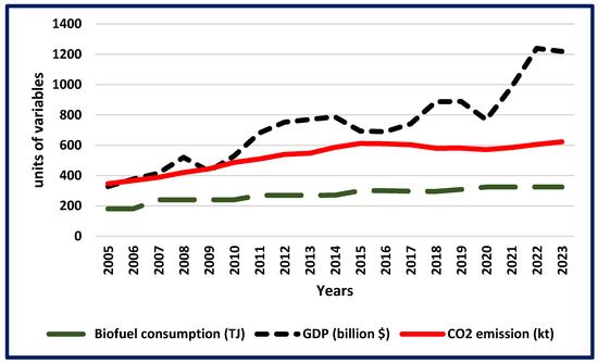
As a preliminary step before conducting cointegration analysis, Figure 1 indicates a potential long-term relationship between biofuel consumption (TJ), gross domestic product (billion $) and CO₂ emission (kt). This visual evidence provides initial support for proceeding and conducting cointegration tests.

Figure 1. Graphic analysis results. Source: Drawn by author.

3.2. Co-Integration Test Analysis Results

3.2.1. The Results of Unit Root Tests

The stability of biofuel consumption ((E), gross domestic product (G) and CO₂ emissions (C) in Saudi Arabia were examined using the unit root test through Augmented Dickey–Fuller (ADF) and Phillips–Perron (PP) tests. All series are stationary at 1(1) and science ADF Statistics were significant at 1% level in the first difference, signifying that the chains are stationary at 1(1) (Table 3 and Table 4). Accordingly, the series appear in the same fixed order, and therefore the Engle–Granger test was elected to measure the association among the chains.

Table 3. Results of unit root test (ADF).

Time Series	Intercept	Intercept and Trend	Stationarity	Intercept	Intercept and Trend	Stationarity
	At Level			At First Difference
LE	−2.261	−2.388	Non stationary	−3.752 *	−6.033 *	Stationary
LG	−0.186	−2.138	Non stationary	−5.344 *	−5.281 *	Stationary
LC	−1.247	−2.401	Non stationary	−1.619	−4.603 *	Stationary

* at 1% level of significance. E, G and C are biofuel consumption, gross domestic product and CO₂ emissions, respectively. L represents logarithm.

Table 4. Results of unit root test (Phillips–Perron (PP)).

Time Series	Intercept	Intercept and Trend	Stationarity	Intercept	Intercept and Trend	Stationarity
	At Level			At First Difference
LE	−3.146	−3.116	Non stationary	−6.724 *	−6.595 *	Stationary
LG	−0.100	−2.138	Non stationary	−5.345 *	−5.272 *	Stationary
LC	−1.707	−0.359	Non stationary	−4.096 *	−4.737 *	Stationary

* At 1% level of significance. E, G and C are biofuel consumption, gross domestic product and CO₂ emissions, respectively. L represents logarithm.

3.2.2. Part One: Cointegration Analysis Results (Biofuel Consumption and Gross Domestic Product)

The ADF tests concentrated on the residuals (i_t) and (z_t) in Equations (3) and (4), respectively (Table 5). The table shows that ADF statistics are −3.82 and –5.77, statistically significant at 1% level of significance. The outcomes combined to confirm the alternative hypothesis of integration, demonstrating that the biofuel consumption and gross domestic product possess long-run association. This result matched with a previous study [29]. This study explores the long-term associations among renewable energy consumption, economic growth, and environmental sustainability in Saudi Arabia from 1990 to 2023, using the ARDL model. The results confirm the presence of cointegration, reflecting the dynamic interaction between renewable energy, economic growth, and environmental sustainability [34].

Table 5. Cointegration Test—Engle–Granger test results—ADF residual (LE and LG).

Dependent	LG	LE
LE	−3.82 *
LG		−5.77 *

* Indicates 1% level of significance. E and G represent biofuel consumption and gross domestic product, respectively. L represents logarithm.

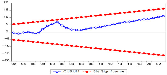
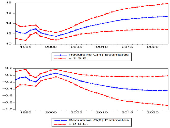
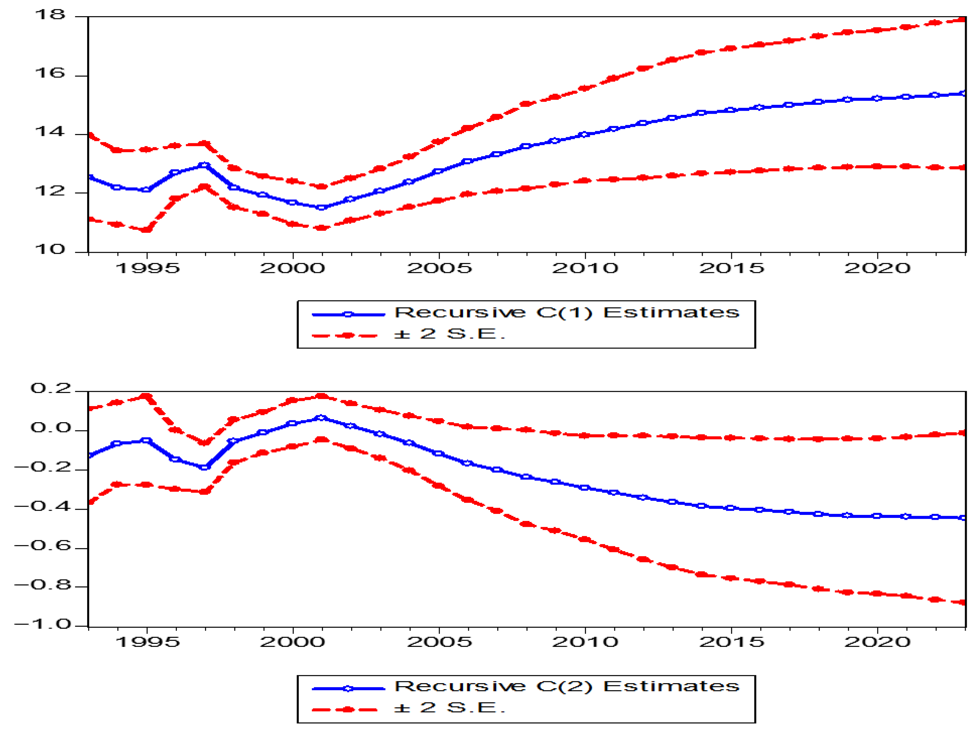
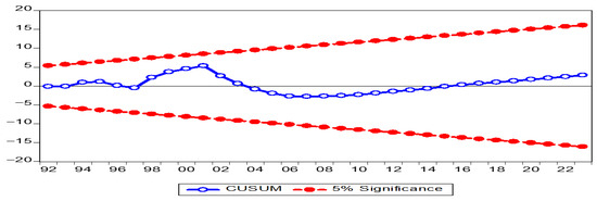
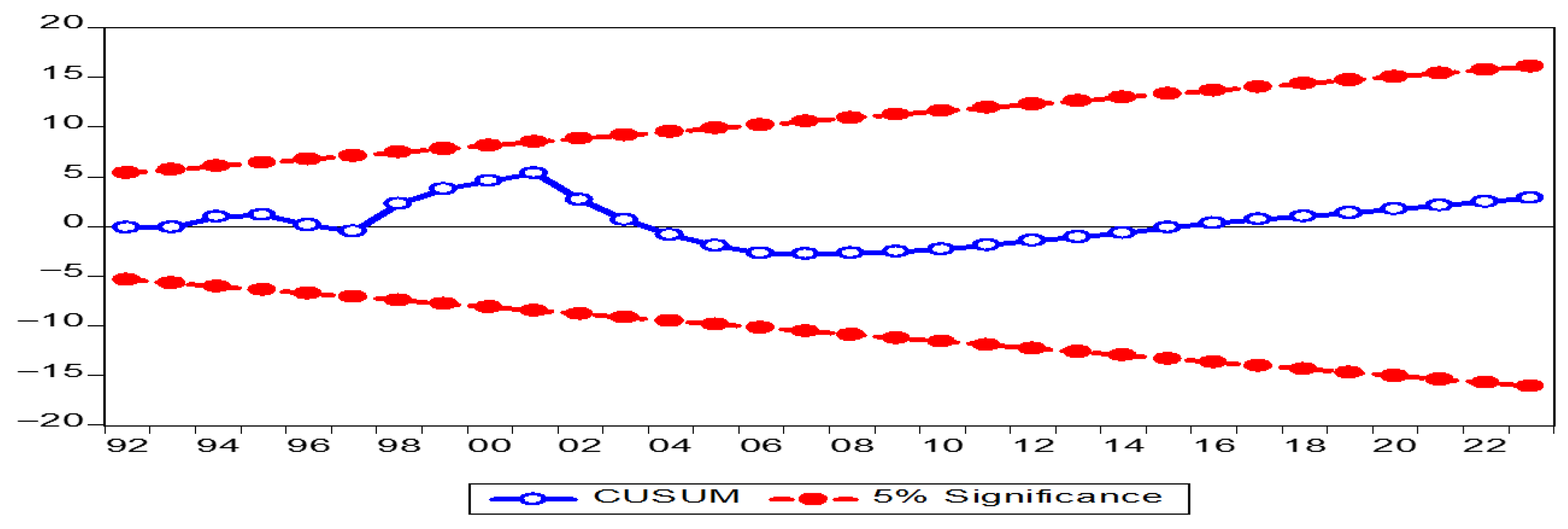
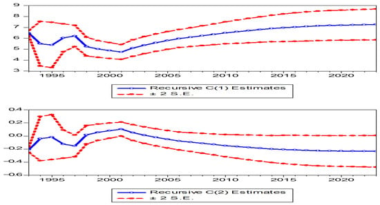
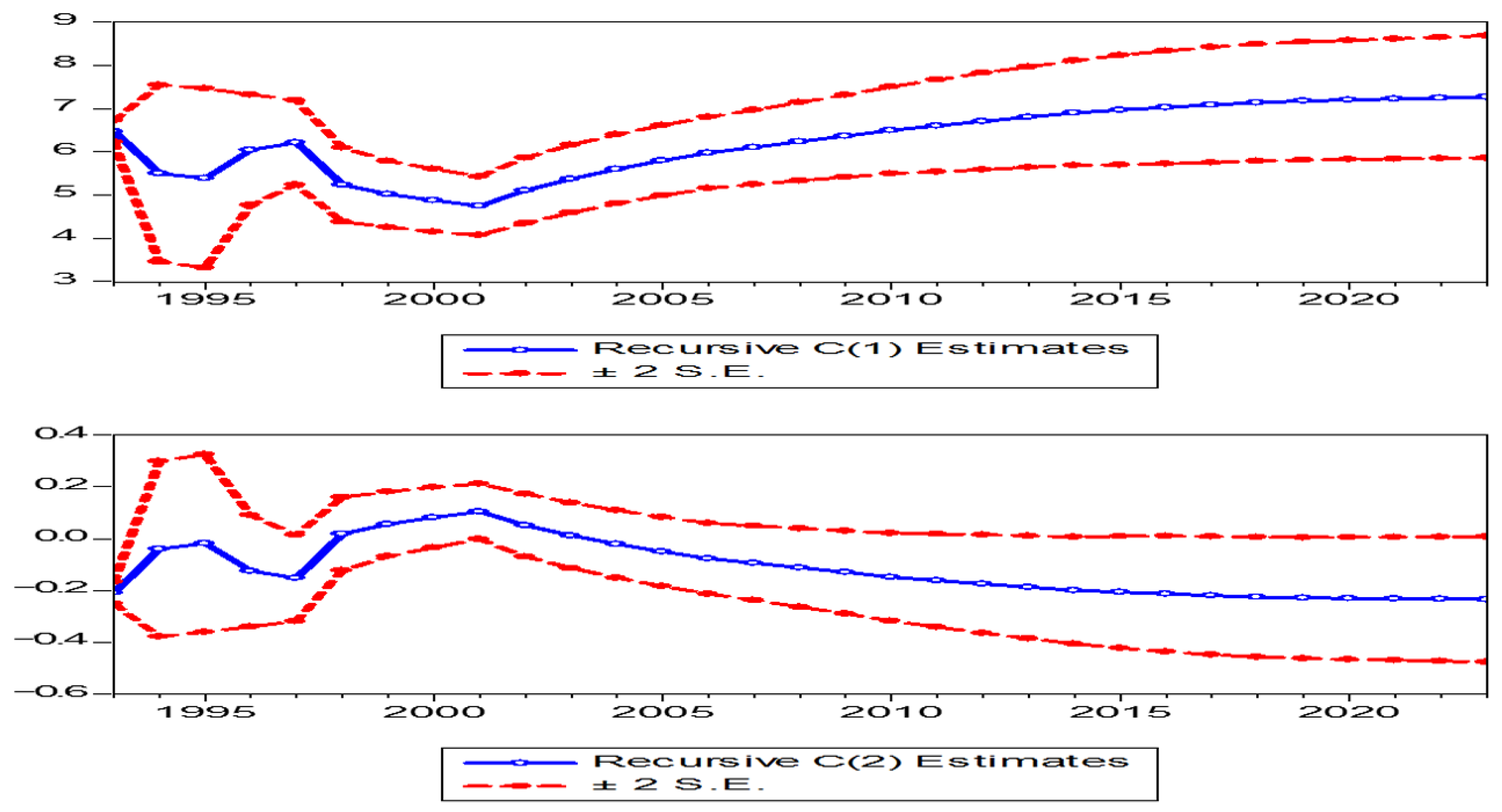
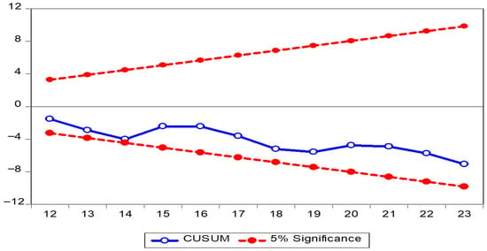
To strength the results of the Engle–Granger test, residual diagnostics and the Chow test were used (Table 6). Jarque–Bera statistic equals 3.61, Prob. = 0.17 and 2.58, Prob. = 0.28 foe models 1 and 2, respectively, suggesting that the residuals are normally distributed. Chow Forecast F-statistic equals 0.21, Prob. = 0.98 and 2.86, Prob. = 0.022 for models 1 and 2, respectively. This result suggests that the structure breaks are absent and present in models 1 and 2, respectively. In addition, stability tests were checked by CUSUM and recursive coefficient estimates for models 1 and 2, respectively, indicating the stability of the models (Figure 2 and Figure 3). Figure 3 shows recursive coefficient estimates, which are used to test parameter stability in the regression model. The figure showed the stability of the model, since the coefficient (blue line) stays within the confidence bands (red lines).

Table 6. Stability diagnostics results of the Engle–Granger test LE and LG.

Accuracy Tools	LE (Dependent) Model 1	LG (Dependent) Model 2
Jarque–Bera statistic	3.61, Prob. = 0.17	2.58, Prob. = 0.28
Chow Forecast Test	F-statistic = 0.21, Prob. = 0.98	F-statistic = 2.86, Prob. = 0.022

E and G represent biofuel consumption and gross domestic product, respectively. L represents logarithm.

Figure 2. CUSUM curve (biofuel consumption as dependent and GDP independent). Source: Drawn by author.

Figure 3. Recursive estimates curve (GDP as dependent and biofuel consumption independent). Source: Drawn by author.

Also, alternative cointegration methods (fully modified ordinary least squares (FMOLS) and dynamic ordinary least squares (DOLS)) were used to robustness of the Engle–Granger test results (Table 7 and Table 8).

Table 7. Results of robustness test: fully modified ordinary least squares (FMOLS).

LE (Dependent Variable)		LG (Dependent Variable)
Independent V.	Coefficient	Independent V.	Coefficient
LG	−0.24 (0.07)	LE	−0.74 (0.06)
C	8.95 (0.00)	C	17.10(0.00)
R-squared 0.09 Adj. R-squared 0.06		R-squared 0.92 Adj. R-squared 0.91
arque–Bera test: 4.26 Prob. 0.12		Jarque–Bera test: 0.40 Prob.0.82

Statistics concerning ( ) are Probability. E and G are biofuel consumption and gross domestic product, respectively. L represents logarithm.

Table 8. Results of robustness test: dynamic ordinary least squares (DOLS) (LE and LG).

LE (Dependent Variable)		LG (Dependent Variable)
Independent V.	Coefficient	Independent V.	Coefficient
LG	−1.85 (0.007)	LE	1.71 (0.07)
C	29.39 (0.005)	C	3.62 (0.42)
R-squared 0.98 Adj. R-squared 0.90		R-squared 0.99 Adj. R-squared 0.96
Jarque–Bera test: 0.95 Prob. 0.62		Jarque–Bera test: 0.40 Prob.0.82

Statistics inside ( ) are Probability. E and G are biofuel consumption and gross domestic product, respectively. L represents logarithm.

Long run confirmation: Fully modified ordinary least squares (FMOLS) and dynamic ordinary least squares (DOLS) were run to reinforce the findings of the Engle–Granger test [53]. Table 7 and Table 8 display the findings of FMOLS and DOLS models, respectively.

The results of fully modified ordinary least squares (FMOLS) and dynamic ordinary least squares (DOLS) are synchronized with Engle–Granger test valuation (Table 9). We found that biofuel consumption and economic growth possess long-run association. Many preceding studies used fully modified ordinary least squares (FMOLS) and dynamic ordinary least squares (DOLS) to fortify the findings of integration models, specifically the ARDL model [39,54].

Table 9. Long-run evidence (LE and LG).

Dependent–Independent	Engle–Granger	FMOLS	DOLS
LE-LG	−3.82 *	−0.24 ***	−1.85 *
LG-LE	−5.77 *	−0.74 ***	1.71 ***

Source: Table 5, Table 6 and Table 7. * and *** significance level at 1% and 10%, respectively; E—biofuel consumption in Saudi; G—gross domestic product; FMOLS—fully modified ordinary least squares; DOLS—dynamic ordinary least squares; L—logarithm.

3.2.3. Results of ECM (Biofuel Consumption and Economic Growth)

Table 10 identifies the optimal lag 1, which is required for running the ECM. The findings of ECM are presented in Table 11. To validate the Vector Error Correction Model (VECM) and ensure its reliability, residual diagnostic tests specifically VEC residual normality tests, serial correlation LM tests, and the Jarque–Bera statistic were used [50]. The LM- statistic (lag 1) equals 1.44 with Prob. = 0.84, signifying no serial correlation. The VEC Residual Normality Tests and Jarque–Bera statistics equal Chi-sq = 1.57 (prob. 0.46) and 0.43 (prob. 0.81), demonstrating that the residual is normality distributed. Therefore, the outcomes of model capability focused to castoff of null hypothesis, no serial correlation and normal distribution of residuals. The estimate of correction factor for biofuel consumption (as dependent variable) showed negative sign −0.61 and significant (critical t-value = −3.20), concluding that the model was capable to accurate its preceding time variability. Also, the findings suggest that the estimate of adjustment parameter gross domestic product (as dependent variable) was negative (−0.02) and statistically insignificant (critical t-value = −0.50), signifying that the model was powerless to accurate its past period variability. This outcome determined that the models might need more time than a year to accurate its former time disparity.

Table 10. Lag selection between variables LE and LG.

Lag	LogL	LR	FPE	AIC	SC	HQ
0	−63.96	NA	0.21	4.12	4.21	4.15
1	1.47	116.98 *	0.01 *	0.34 *	0.61 *	0.43 *

Where *—Lag order selected by the criterion; NA—not available; FPE—final prediction error; SC—Schwarz information criterion; LR—sequential modified likelihood ratio (LR) test statistic (each test at 5% level); HQ—Hannan–Quinn inf n information criterion; AIC—Akaike information criterion; logL—log lag variable.

Table 11. Results of ECM (biofuel consumption and gross domestic product).

Error Correction	D(LE)	D(LG)
CointEq1	−0.61 [−3.20]	−0.02 [−0.50]
D(LE(−1))	0.21 [1.10]	−0.01 [0.29]
D(LG(−1))	−0.02 [−0.2]	0.01 [0.03]
C	−0.01 [−0.09]	0.07 [2.62]
VEC Residual Normality Tests: Chi-sq = 1.57		Prob. = 0.46
Jarque–Bera statistic: 0.43		Prob. = 0.81
ECM residual serial correlation LM tests: Lags	LM-Stat	Prob.
1	1.44	0.84

Figures between [] are critical t-values. E and G are biofuel consumption and gross domestic product, respectively. L represents logarithm.

3.2.4. Part Two: Co-Integration Analysis Results (Biofuel Consumption and CO₂ Emission)

At first difference ADF and PP estimates of biofuel consumption and CO₂ emission are significant at 1% level, demonstrating that the same stationary order 1(1) (Table 3 and Table 4). The ADF and PP tests were applied on the residuals (i_t) and (z_t) in Equations (5) and (6), respectively (Table 12). ADF estimates of biofuel consumption and CO₂ emission equal −3.77 and −4.44 which are statistically significant at 1% level, suggesting that biofuel consumption and CO₂ emission bond in the long run. This result harmonized with previous studies [33,34].

Table 12. Cointegration Test—Engle–Granger test results—ADF residual(LE and LC).

Dependent	LC	LE
LE	−3.77 *
LC		−4.44 *

Source: Author calculations. * indicates 1% level of significance. E and C are biofuel consumption and CO₂ emission, respectively. L represents logarithm.

Long-run confirmation

Jarque–Bera statistic equals 3.61, Prob. = 0.17 and 2.58, Prob. = 0.28 foe mode 1 and 2, respectively, suggesting that the residuals are normally distributed (Table 13). From the Table 13, Chow Forecast F-statistic equals 0.21, Prob.= 0.98 and 2.86, Prob. = 0.022 for model 1 and 2, respectively. This result suggests that the structure breaks are absent and present in models 1 and 2, respectively. In addition, stability tests are checked by CUSUM and CUSUMSQ for model 1 and 2, respectively, indicating the stability of the models (Figure 4 and Figure 5). Figure 6 is recursive coefficient estimates, which are used to test parameter stability in the regression model. The figure shows the stability of the model, since the coefficient stays within the confidence bands. Also, alternative cointegration methods (fully modified ordinary least squares (FMOLS) and dynamic ordinary least squares (DOLS)) were used (Table 14 and Table 15).

Table 13. Stability diagnostics results of the Engle–Granger test LE and LC.

Accuracy Tools	LE (Dependent) Model 1	LC (Dependent) Model 2
Jarque–Bera statistic	5.57, Prob. = 0.06	2.96, Prob. = 0.23
Chow Forecast Test	F-statistic = 0.11, Porb. = 0.99	F-statistic = 2.05, Porb. = 0.08

E and C are biofuel consumption and CO₂ emission, respectively. L represents logarithm.

Figure 4. CUSUM curve (biofuel consumption as dependent and CO₂ independent variable). Source: Drawn by author.

Figure 5. Recursive estimates curve (CO₂ as dependent and biofuel consumption independent). Source: Drawn by author.

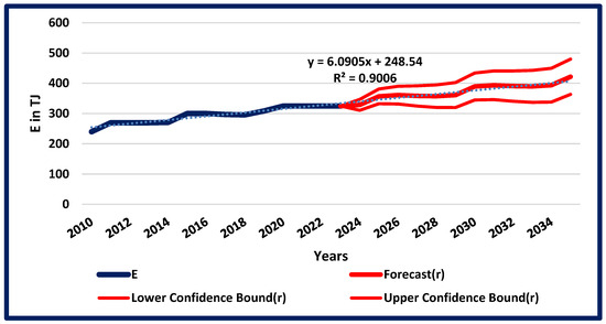
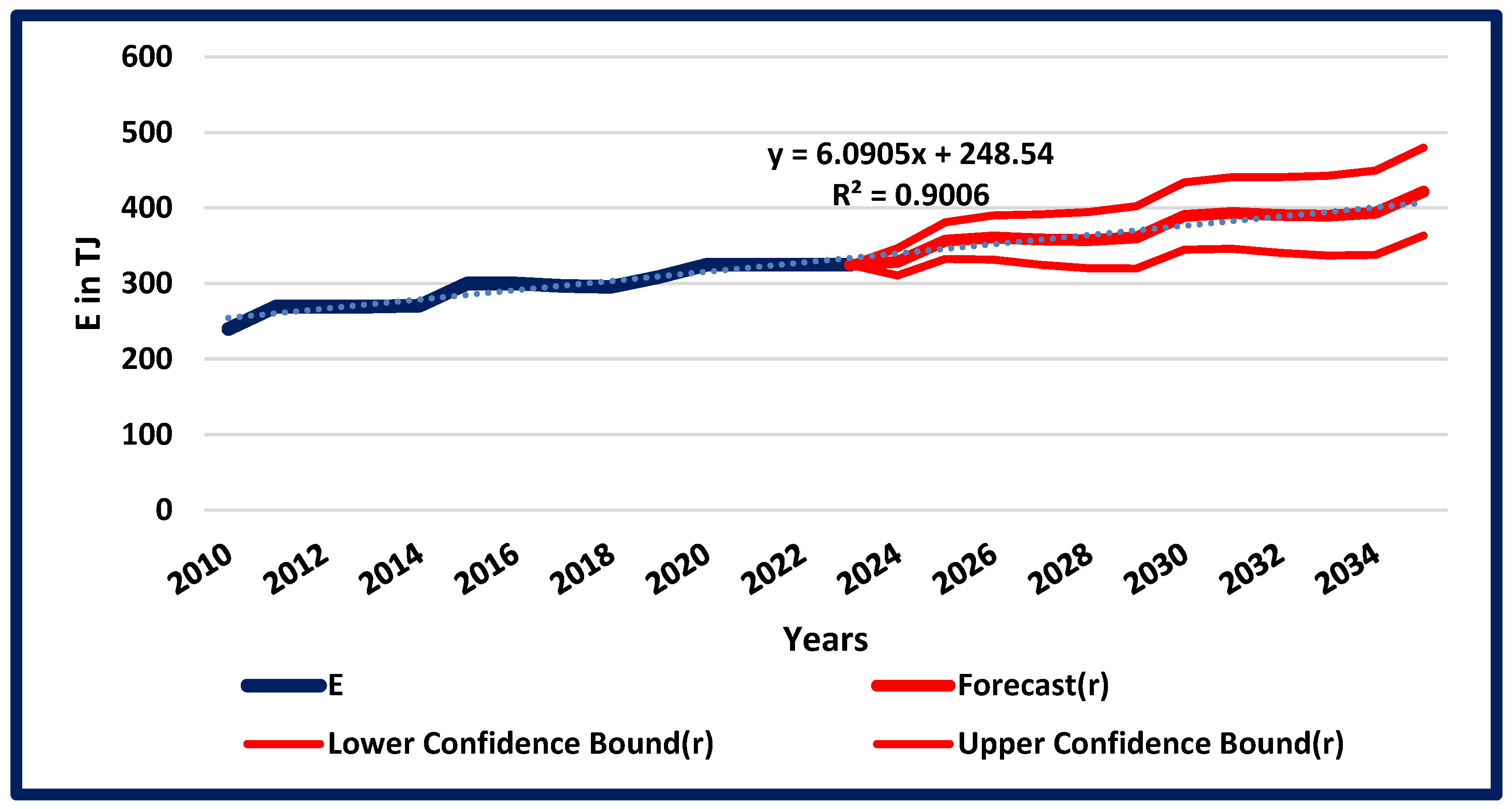
Figure 6. Forecasting graph (E: biofuel consumption). Source: Drawn by author.

Table 14. Results of robustness test: FMOLS—fully modified ordinary least squares.

LE (Dependent Variable)		LC (Dependent Variable)
Independent V.	Coefficient	Independent V.	Coefficient
LC	−0.47 (0.06)	LE	−0.39 (0.07)
C	8.63 (0.000)	C	8.20 (0.000)
R-squared 0.08 Adj. R-squared 0.05		R-squared 0.03 Adj. R-squared −0.01
Jarque–Bera test: 4.83 Prob. 0.10		Jarque–Bera test: 3.41 Prob.0.18

Statistics inside ( ) are Probability. E and C are biofuel consumption and CO₂ emission, respectively. L represents logarithm.

Table 15. Results of robustness Test: dynamic ordinary least squares (DOLS).

LE (Dependent Variable)		LC (Dependent Variable)
Independent V.	Coefficient	Independent V.	Coefficient
LC	−0.67 (0.09)	LE	2.18 (0.004)
C	10.06 (0.000)	C	−6.18 (0.02)
R-squared 0.17 Adj. R-squared 0.05		R-squared 0.99 Adj. R-squared 0.98
Jarque–Bera test: 5.01 Prob. 0.10		Jarque–Bera test: 2.19 Prob.0.34

Figures between ( ) are Probability. E and C are biofuel consumption and CO₂ emission, respectively. L represents logarithm.

The findings of fully modified ordinary least squares (FMOLS) and dynamic ordinary least squares (DOLS) appeared in Table 14 and Table 15, respectively.

The findings of fully modified ordinary least squares (FMOLS) and dynamic ordinary least squares (DOLS) are similar to the Engle–Granger calculation (Table 16). A long-run association was detected among biofuel consumption and CO₂ emission.

Table 16. Long-run evidence of Engle–Granger test between LE and LC.

Dependent–Independent	Engle–Granger	FMOLS	DOLS
LE-LC	−3.77 *	−0.47 ***	−0.67 ***
LC-LE	4.44 *	−0.39 ***	2.18 *

Source: Table 12, Table 14 and Table 15. * and *** significance level at 1% and 10%, respectively. All abbreviations are illustrated in Table 9. E and C are biofuel consumption and CO₂ emission, respectively. L represents logarithm.

3.2.5. Results of ECM (Biofuel Consumption and CO₂ Emission)

Lag length 1 was selected (Table 17). From Table 18, residual diagnostic tests results showed that the ECM residual serial correlation LM- estimate (lag 1) equals 5.80 with Prob.= 0.22, signifying no serial correlation. Jarque–Bera statistics and the VEC Residual Normality tests equal 1.69 (prob. 0.43) and Chi-sq = 1.57 (prob. 0.46), representing that the normality distribution of the residual. Consequently, these outcomes of model suitability concentrating to castoff of null hypothesis, no serial correlation and normal distribution of residuals. The correction factor estimates for biofuel consumption (as dependent variable) shown negative sign (−0.63) and significant (critical t-value= −3.27), signifying that the model was capable to true its prior period variability. This outcome harmonized with a previous study [29]. The study showed that renewable energy consumption had a statistically significant negative impact on short-term carbon dioxide emissions. Likewise, the outcomes of CO₂ emission suggest that the adjustment parameter estimates were negative (0.02) and statistically insignificant (critical t-value= −1.36), demonstrating that the model was incapable to precise its former period variability.

Table 17. Lag selection between LE and LC.

Lag	LogL	FPE	AIC	HQ	SC	LR
1	39.04	0.0004 *	−2.19 *	−2.13 *	−2.01 *	NA
2	41.91	0.0004	−2.12	−1.99	−1.75	5.02

Source: Author calculations based on collected data. All abbreviations are illustrated in Table 10. * indicates 1% level of significance.

Table 18. Results of ECM (biofuel consumption and CO₂ emission).

Error Correction	D(LE)	D(LC)
CointEq1	−0.63 [−3.27]	−0.02 [−1.36]
D(LE(−1))	0.24 [1.24]	−0.0001 [−0.01]
D(LC(−1))	−3.57 [−1.15]	0.25 [1.37]
C	0.13 [0.84]	0.03 [3.33]
VEC Heteroskedasticity Test: 21.27 Prob.		0.27
ECM residual serial correlation LM tests: Lags	LM-Stat	Prob.
1	5.80	0.22
Jarque–Bera statistic: 1.69		Prob.= 0.43
VEC Residual Normality Tests: Chi-sq = 1.57		Prob.= 0.46

Numbers regarding [] are critical t-values. E and C are biofuel consumption and CO₂ emission, respectively. L represents logarithm.

3.2.6. Forecasting Analysis Result

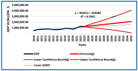
Linear forecast models were applied. The model tests its accuracy through residual diagnostic test, stability diagnostics CUSUM and CUSUM of Square test and structural break tests (Chow Forecast Test) are run to justify parameter stability (Table 19). Generally, in the forecasting graph the blue and red part reflect to actual and prediction for the period, respectively.

Table 19. Stability diagnostics results of the forecast models for E, G and C.

Accuracy Tools	E	G	C
Heteroskedasticity Test: Breusch–Pagan–Godfrey	F = 1.80, Prob. = 0.20	F = 3.38, Prob. = 0.10	F = 1.89, Prob. = 0.19
Jarque–Bera statistic	0.48, Prob. = 0.79	0.37, Prob. = 0.83	0.82, Prob. = 0.66
Residual serial correlation LM tests	F = 0.02, Prob. = 0.89	F = 3.27, Prob. = 0.10	F = 10.36, Prob. = 0.01
Chow Forecast Test	F-statistic = 0.45, Porb. = 0.84	F-statistic = 2.50, Porb. = 0.19	F-statistic = 24.63, Porb. = 0.004

E, G and C are biofuel consumption, gross domestic product and CO₂ emission, respectively.

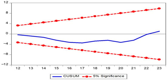
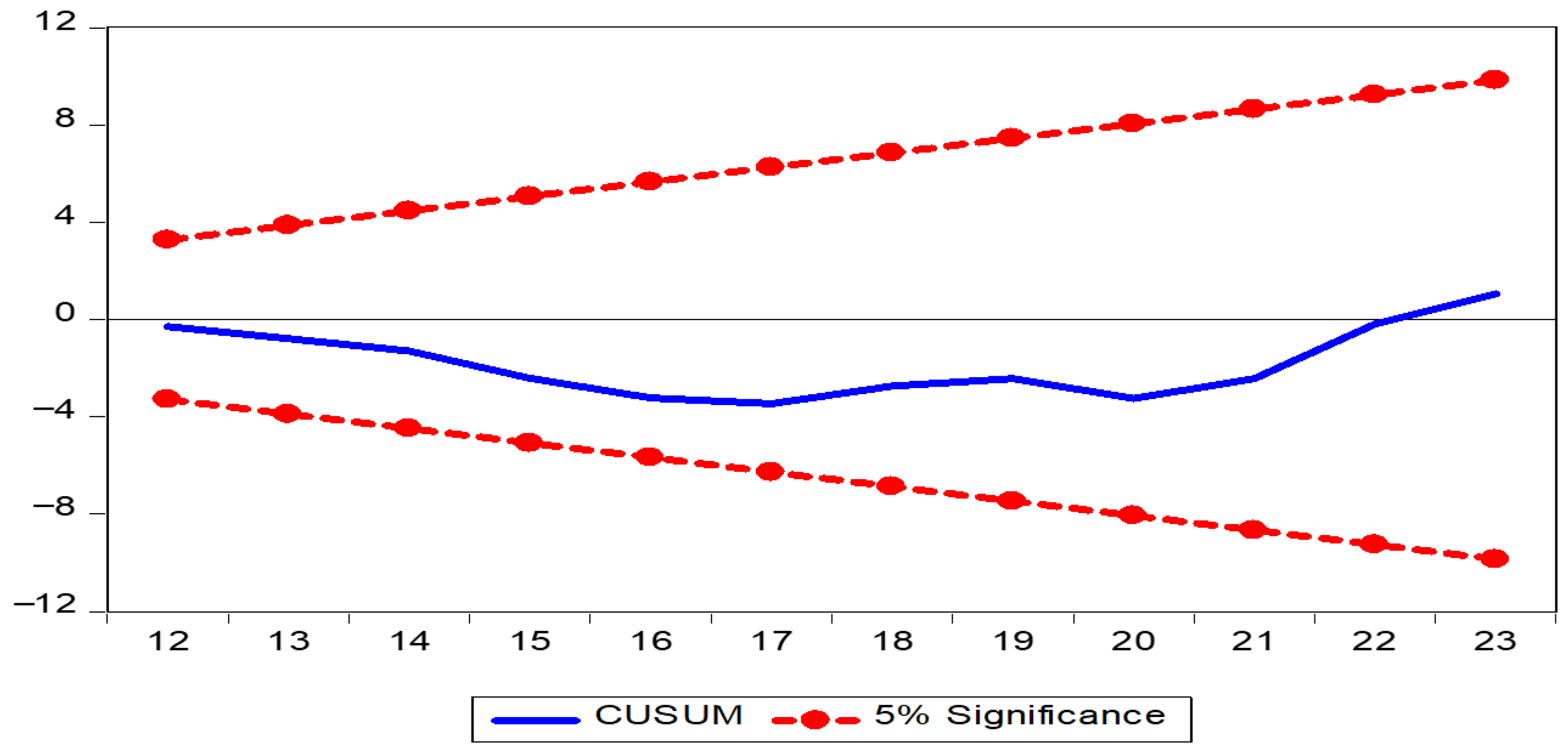
Graph 6 looked validity by various predicting indicators: Mean Square Error, Alph, Beta and Gamma equal to 0.79, 0.9, 0.0 and 0.10, respectively. Also, the growth rates of biofuel consumption equal to 2.40% and 2.80% for the period 2010 to 2023 and prediction period 2023 to 2035, respectively, ending that there is increasing in biofuel consumption by 2.80% in Saudi during the forecast period. To ensure model reliability (the Table 19), residual diagnostic tests specifically serial residual correlation LM tests and the Jarque–Bera statistic were used. The LM- statistic equals 0.02 with Prob. = 0.89, signifying no serial correlation. Jarque–Bera statistics equal Chi-sq = 0.48 (prob. 0.79), demonstrating that the residual is normality distributed. Therefore, the outcomes of model capability focused to castoff of null hypothesis, no serial correlation and normal distribution of residuals. Heteroskedasticity statistic Test equals 1.80 with prob. = 0.20, meaning that the residuals are homoskedastic (constant variance) and the model is well specified in terms of variance. Reference to structural break tests, Chow Forecast test result F-statistic = 0.45 with Porb. = 0.84 (more than 0.5), justifying the parameter stability. Since, The CUSUM line stays within the confidence bands, CUCUM curve indicated that the model parameters are stable over the study period, meaning that on indication of structural breaks (Figure 7).

Figure 7. CUCUM curve (biofuel consumption). Source: Drawn by author.

Also, Figure 8 looked validity by various forecasting indicators: Mean Square Error, Alph, Beta and Gamma equal to 2.17, 1.00, 0.25 and 0.00, respectively. Also, the growth rates of gross domestic product equal to 7.50% and 11.00% for the period 2010 to 2023 and the prediction period 2023 to 2035, respectively, demonstrating that there is increasing gross domestic product but at decreasing rate (11.00%) during forecast period. This outcome harmonized to some extend with prior study in that GDP performance in future will increased [55]. The authors found that The forecast equal to 1.3% in 2023. To ensure model reliability (the Table 19), residual diagnostic tests specifically residual normality tests, serial correlation LM tests, and the Jarque–Bera statistic were used. The LM- statistic equals 3.27 with Prob.= 0.10, signifying no serial correlation. Jarque–Bera statistics equal Chi-sq = 0.37 (prob. 0.83), demonstrating that the residual is normality distributed. Therefore, the outcomes of model capability focused to castoff of null hypothesis, no serial correlation and normal distribution of residuals. Heteroskedasticity statistic Test equals 3.38 with prob.= 0.10, meaning that the residuals are homoskedastic (constant variance) and the model is well specified in terms of variance. Reference to structural break tests, Chow Forecast test result F-statistic = 2.50 with Porb. = 0.19 (more than 0.5), justifying the parameter stability. Since, The CUSUM line stays within the confidence bands, CUCUM curve indicated that the model parameters are stable over the study period, meaning that on indication of structural breaks (Figure 9).

Figure 8. Forecasting graph (GDP in billion $). Source: Drawn by author.

Figure 9. CUCUM curve (GDP). Source: Drawn by author.

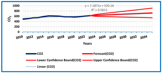
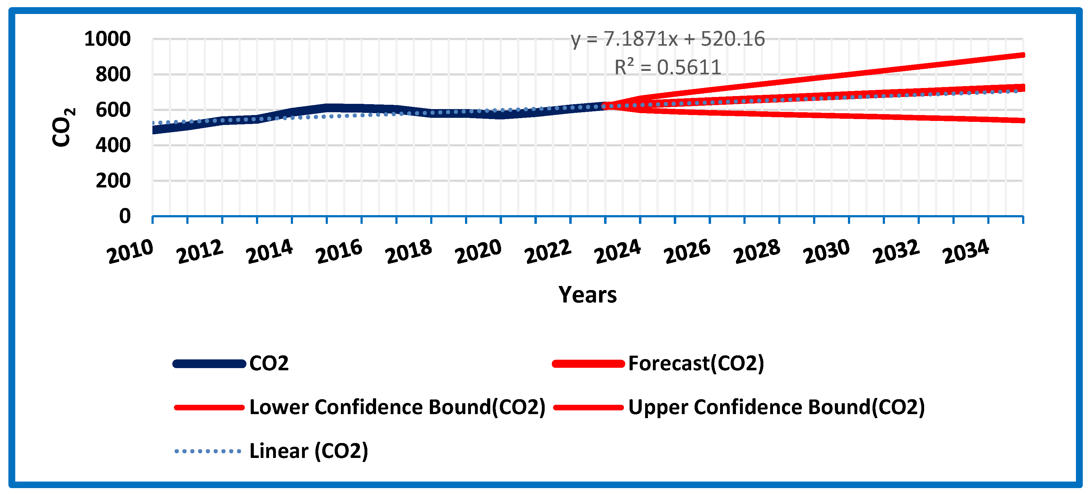
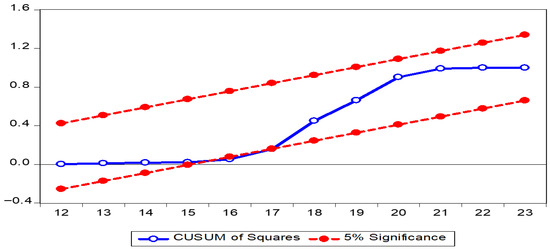
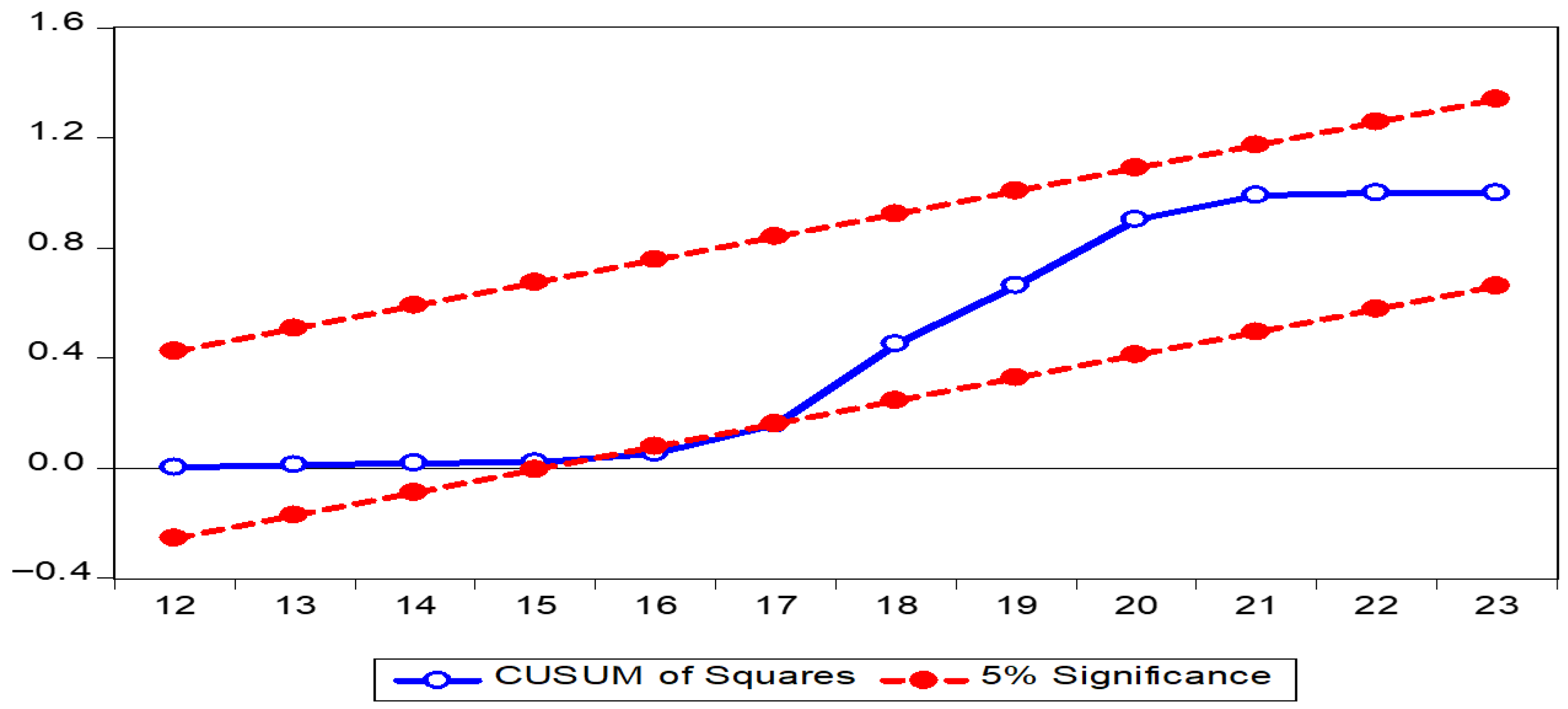
Moreover, Figure 10 showed validity by statistics of predicting pointers: Mean Square Error, Alph, Beta and Gamma equal to 0.58, 1.0, 0.10 and 0.00, respectively. Also, the growth rates of CO₂ equal to 1.90% and (0.95%) for the period 2010 to 2023 and the prediction period 2023 to 2035, respectively, finishing that there is increasing in CO₂ emissions but at reducing rate (0.95%) throughout prediction period. This result matched with a previous study which delivers valuation of Saudi Arabia’s actions to achieve the goal of reaching net zero emissions by 2060 [56]. This paper delivers valuation of Saudi Arabia’s actions to achieve the goal of reaching net zero emissions by 2060. Founded on the results, Saudi Arabia will see a substantial decrease in emissions after 2030, when renewable energy schemes are finalized. Its exposes that Saudi Arabia will decrease its total net emissions to 49.67 million tons of carbon dioxide equivalent. Jarque–Bera statistics equal Chi-sq = 0.82 (prob. 0.66), demonstrating that the residual is normality distributed. Therefore, the outcomes of model capability focused to castoff of null hypothesis, no serial correlation and normal distribution of residuals. Heteroskedasticity statistic Test equals 1.89 with prob.= 0.19, meaning that the residuals are homoskedastic (constant variance) and the model is well specified in terms of variance. In addition, Chow Forecast Test statistic equals 24.63 with Prob. = 0.004 (less than 0.05), meaning that there is the significant change in the relationship between variables during 2016. This result may be reflecting to Launch of Saudi Vision 2030 and oil price collapse. The CUSUM Square line stays within the critical bounds, indicating that the model parameters are stable during study period and suggestion of structural breaks (Figure 11).

Figure 10. Forecasting graph (CO₂). Source: Drawn by author.

Figure 11. CUSUM of Squares (CO₂). Source: Drawn by author.

4. Discussion

This study examines the impact of biofuel consumption on economic growth and environmental quality. The analysis consists of two parts: the first investigates the cointegration link between biofuel consumption and GDP, while the second assesses the long-term relationship between biofuel consumption and CO₂ emissions. The research also includes a forecasting component. Data on biofuel consumption, economic growth, and CO₂ emissions were composed from multiple sources covering the period from 1990 to 2023. Engle–Granger cointegration tests confirm the existence of long-term relationships between biofuel consumption, economic growth, and environmental quality. Estimates obtained using FMOLS and DOLS methods are consistent with the Engle–Granger results, thus enhancing the robustness of the findings. The growth rate of biofuel consumption is estimated at 2.40% for the period 2010–2023 and is projected to rise to 2.80% during the period 2023–2035. Similarly, GDP growth rates are estimated at 7.50% for the period 2010–2023 and are projected to rise to 11.00% during the forecast period 2023–2035. In contrast, CO₂ emissions grew by 1.90% between 2010 and 2023, but this growth is expected to slow to 0.95% between 2023 and 2035. These findings suggest that biofuel consumption is likely to continue expanding at a relatively rapid pace, accompanied by strong economic growth and slowdown in CO₂ emissions. The results highlight the importance of promoting biofuel development and implementing clean energy policies to support sustainable economic growth while reducing emissions in the long term.

References

- Frankowski, J.; Czekała, W. Environmentally Friendly Biofuel Production. Energies 2024, 17, 5370. [Google Scholar] [CrossRef] [Scilit]
- Mizik, T.; Igbeghe, C.B.; Deák, Z. Production Efficiency of Advanced Liquid Biofuels: Prospects and Challenges. Energy 2025, 18, 1008. [Google Scholar] [CrossRef] [Scilit]
- Xiong, Q.; Duan, Y.; Liang, D.; Li, T.; Luo, H.; Chen, R. Biofuels and Their Blends—A Review of the Effect of Low Carbon Fuels on Engine Performance. Sustainability 2024, 16, 10300. [Google Scholar] [CrossRef] [Scilit]
- Baloyi, S.F. The Impact of Renewable Energy Consumption, Foreign Direct Investment, Economic Growth, and Carbon Dioxide Emissions on Soybean Production in South Africa (Order No. 32026654). Master’s Thesis, University of South Africa, Pretoria, South Africa, 2024. Available online: https://www.proquest.com/dissertations-theses/impact-renewable-energy-consumption-foreign/docview/3224598965/se-2 (accessed on 5 February 2026).
- Borthakur, P.P.; Borthakur, B. The role of industrial catalysts in accelerating the renewable energy transition. Chem. Proc. 2025, 17, 6. [Google Scholar] [CrossRef] [Scilit]
- Triki, R.; Mahmoud, S.M.; Bahou, Y.; Boudabous, M.M. Assessing Renewable Energy Adoption to Achieve Sustainable Development Goals in Ha’il Region. Sustainability 2025, 17, 6097. [Google Scholar] [CrossRef] [Scilit]
- Yacout, D.M.; Tysklind, M.; Upadhyayula, V.K. Socio-economic implications of forest-based biofuels for marine transportation in the Arctic: Sweden as a case study. Front. Clim. 2024, 6, 1414813. [Google Scholar] [CrossRef] [Scilit]
- Saleem, M.; Ali, M.; Bin-saleem, M.; Saleem, M.T.B. Artificial photosynthesis a novel and sustainable renewable energy source: In the perspective of Saudi Arabia. Clean Energy Technol. J. 2023, 1, 90–104. [Google Scholar] [CrossRef] [Scilit]
- KSA Vision 2030. Strategic Objectives and Vision Realization Programs, Saudi Vision 2030. 2019. Available online: https://www.vision2030.gov.sa/media/rc0b5oy1/saudi_vision203.pdf?utm (accessed on 10 December 2025).
- Ministry of Environment Water and Agriculture. Executive Regulation for Logging For the Environmental Law Issued by the Royal Decree. 2020, No. (m/165), Dated 19/11/1441Hijri. Available online: https://www.mewa.gov.sa/en/InformationCenter/DocsCenter/RulesLibrary/Docs/Executive%20Regulation%20for%20Logging.pdf (accessed on 5 February 2026).
- INDEXBOX Wood Fuel-Saudi Arabia. 2026. Available online: https://app.indexbox.io/table/440110h440112/682/?_gl=1*1cth0rj*_ga*MTI1MTI3OTQ5Ny4xNzcwMTc2MzI4*_ga_6KCVGEDSJE*czE3NzAyNjY4ODQkbzIkZzEkdDE3NzAyNjgxMjgkajQ4JGwwJGgw (accessed on 5 February 2026).
- Worldbank. Saudi Arabia Wood Charcoal Imports by Country in 2023. 2023. Available online: https://wits.worldbank.org/trade/comtrade/en/country/SAU/year/2023/tradeflow/Imports/partner/ALL/product/440200?utm_source=chatgpt.com (accessed on 4 February 2026).
- Kostakis, I.; Armaos, S.; Abeliotis, K.; Theodoropoulou, E. The investigation of EKC within CO2 emissions framework: Empirical evidence from selected cross-correlated countries. Sustain. Anal. Model. 2023, 3, 100015. [Google Scholar] [CrossRef] [Scilit]
- Rabbi, M.F.; Abdullah, M. Fossil fuel CO2 emissions and economic growth in the visegrád region: A study based on the environmental kuznets curve hypothesis. Climate 2024, 12, 115. [Google Scholar] [CrossRef] [Scilit]
- Mirziyoyeva, Z.; Salahodjaev, R. Renewable energy, GDP and CO2 emissions in high-globalized countries. Front. Energy Res. 2023, 11, 1123269. [Google Scholar] [CrossRef] [Scilit]
- Muhammed, M.; Saad, S.; Maikudi, Y.I.; Usman, A.B. Dynamic effects of energy consumption and economic growth on CO2 Emission: Testing EKC hypothesis in Africa. ESJ Soc. Sci. 2023, 19, 127. [Google Scholar] [CrossRef] [Scilit]
- Mohamed, E.F.; Abdullah, A.; Jaaffar, A.H.; Osabohien, R. Reinvestigating the EKC hypothesis: Does renewable energy in power generation reduce carbon emissions and ecological footprint? Energy Strategy Rev. 2024, 53, 101387. [Google Scholar] [CrossRef] [Scilit]
- Elmonshid, L.B.E.; Sayed, O.A.; Awad Yousif, G.M.; Eldaw, K.E.H.I.; Hussein, M.A. The impact of financial efficiency and renewable energy consumption on CO2 emission reduction in GCC economies: A panel data quantile regression approach. Sustainability 2024, 16, 6242. [Google Scholar] [CrossRef] [Scilit]
- Alqahtani, R.A. Assessing the impact of economic and energy factors on CO2 emissions: A case study of Saudi Arabia. J. Entrep. Sustain. Issues 2025, 12, 180–188. [Google Scholar] [CrossRef] [Scilit]
- Tlili, H.; Alhamad, S.; Turki, H. How growth, urbanization, and energy consumption affect CO2 emissions in Saudi Arabia (1970–2020)? An ARDL and NARDL approach to investigate the eco-environmental challenge. Energy Strategy Rev. 2025, 59, 101691. [Google Scholar] [CrossRef] [Scilit]
- Alajmi, R.G. Energy consumption and carbon emissions: An empirical study of Saudi Arabia. Sustainability 2024, 16, 5496. [Google Scholar] [CrossRef] [Scilit]
- Matar, W.; Mansouri, N.Y.; Umeozor, E. Energy policy pathways to inform climate policy in Saudi Arabia. J. Clean. Prod. 2024, 445, 141190. [Google Scholar] [CrossRef] [Scilit]
- Bhat, M.Y.; Sofi, A.A.; Sajith, S. Exploring environment-energy-growth nexus in OECD countries: A nonparametric approach. Biomass Convers. Biorefinery 2023, 13, 9929–9942. [Google Scholar] [CrossRef] [Scilit]
- Yuping, L.; Ramzan, M.; Xincheng, L.; Murshed, M.; Awosusi, A.A.; Bah, S.I.; Adebayo, T.S. Determinants of carbon emissions in Argentina: The roles of renewable energy consumption and globalization. Energy Rep. 2021, 7, 4747–4760. [Google Scholar] [CrossRef] [Scilit]
- Shabani, Z.D.; Shahnazi, R.; Sadati, S.M. The effects of spatial spillover of good governance and renewable energy on CO2 emissions. Environ. Dev. Sustain. 2025, 27, 10857–10894. [Google Scholar] [CrossRef] [Scilit]
- Shahnazi, R.; Shabani, Z.D. The effects of renewable energy spatial spillover of CO2 emissions and economic freedom on CO2 emissions in the EU. Renew. Energy 2021, 169, 293–307. [Google Scholar] [CrossRef] [Scilit]
- Yurtkuran, S.; Yıkıcı, A.; Çolak, Ç. Do anti-corruption and renewable energy drive environmental sustainability? testing the ekc hypothesis for G20 countries. Sustain. Dev. 2025, 33, 8511–8526. [Google Scholar] [CrossRef] [Scilit]
- Sultana, T.; Hossain, M.S.; Voumik, L.C.; Raihan, A. Democracy, green energy, trade, and environmental progress in South Asia: Advanced quantile regression perspective. Heliyon 2023, 9, e20488. [Google Scholar] [CrossRef] [Scilit] [PubMed]
- Abbasi, K.R.; Adedoyin, F.F.; Abbas, J.; Hussaine, K. The impact of energy depletion and renewable energy on CO2 emissions in Thailand: Fresh evidence from the novel dynamic ARDL simulation. Renew. Energy 2021, 180, 1439–1450. [Google Scholar] [CrossRef] [Scilit]
- Li, B.; Haneklausb, N. The role of renewable energy fossil fuel consumption urbanization and economic growth on CO2 emissions in China. Energy Rep. 2021, 7, 783–791. [Google Scholar] [CrossRef] [Scilit]
- Manal, A. The role of renewable energy in driving economic transformation and sustainable development in Saudi Arabia. Int. J. Energy Econ. Policy 2025, 15, 364. [Google Scholar] [CrossRef] [Scilit]
- Mahrous, E.N.; Yousufuddin, S.; Saleem, M. Transitioning to Alternative Fuels: A Study on the Feasibility of Synthetic Fuels in Saudi Arabia’s Road Transport Sector, Yanbu. J. Eng. Sci. 2024, 21, 24–38. [Google Scholar] [CrossRef] [Scilit]
- Qiao, H.; Zheng, F.; Jiang, H.; Dong, K. The greenhouse effect of the agriculture-economic growth-renewable energy nexus: Evidence from G20 countries. Sci. Total Environ. 2019, 671, 722–731. [Google Scholar] [CrossRef] [Scilit]
- Mohammed, M.G.A.; Abdel-Gadir, S.E.M.; Alsulami, F.; Mannai, S.; Arfaoui, L.; Alharbi, K.; Qassim, A.A.; Alsafy, M.M. Exploring the effects of renewable energy, energy consumption, and industrial growth on Saudi Arabia’s environmental footprint: An autoregressive distributed lag analysis. Energies 2024, 17, 6327. [Google Scholar] [CrossRef] [Scilit]
- FAO. 2026. Available online: https://www.fao.org/faostat/ar/#data/RFB (accessed on 5 February 2026).
- Countryeconomy.com. 2026a. Available online: https://countryeconomy.com/gdp/saudi-arabia (accessed on 5 February 2026).
- Countryeconomy.com. 2026b. Available online: https://countryeconomy.com/energy-and-environment/co2-emissions/saudi-arabia (accessed on 5 February 2026).
- Emam, A. Climate Change Effect on Dates Productivity in Saudi Arabia: Implications for Food Security. Sustainability 2025, 17, 4574. [Google Scholar] [CrossRef] [Scilit]
- Dickey, D.A.; Fuller, W.A. Distribution of the estimators for autoregressive time series with a unit root. J. Am. Stat. Assoc. 1979, 74, 427–431. [Google Scholar] [CrossRef] [Scilit]
- Emam, A.A. Present and Future: Does agriculture affect economic gross and environment in the Kingdom of Saudi Arabia? J. Agric. Econ.-Czech. Acad. Agric. Sci. 2022, 68, 361–370. [Google Scholar] [CrossRef] [Scilit]
- Phillips, P.C.; Perron, P. Testing for a unit root in time series regression. Biometrika 1988, 75, 335–346. [Google Scholar] [CrossRef]
- Crowder, W.J.; Wohar, M.E. A cointegrated structural VAR model of the Canadian economy. Appl. Econ. 2004, 36, 195–213. [Google Scholar] [CrossRef] [Scilit]
- Ali, S.; Ying, L.; Shah, T.; Tariq, A.; Ali Chandio, A.; Ali, I. Analysis of the nexus of CO2 emissions, economic growth, land under cereal crops and agriculture value-added in Pakistan using an ARDL approach. Energies 2019, 12, 4590. [Google Scholar] [CrossRef] [Scilit]
- Emam, A.A.; Hassan, K. Co-integration and Market Integration: An Application to Millet Markets in Darfur States, Sudan. Univ. Khartoum J. Agric. Sci. 2002, 10, 277–289. [Google Scholar]
- Emam, A.A. Saudi fertilizers and their impact on global food security: Present and future. Sustainability 2023, 15, 7614. [Google Scholar] [CrossRef] [Scilit]
- Hualde, J.; Olmo, J. A novel test of economic convergence in time series. Empir. Econ. 2025, 68, 2093–2118. [Google Scholar] [CrossRef] [Scilit]
- Venujayakanth, B.; Dudhat, A.S.; Swaminathan, B.; Ardeshana, N.J. Price integration analysis of major groundnut domestic markets in India. Econ. Aff. 2017, 62, 233–241. [Google Scholar] [CrossRef] [Scilit]
- Dhungel, K.R. Estimation of short and long run equilibrium coefficients in error correction model: An empirical evidence from Nepal. Int. J. Econom. Financ. Manag. 2014, 2, 214–219. [Google Scholar] [CrossRef]
- Al-Abdoulhadi, I.A.; Al-Ali, S.; Khurshid, K.; Al-Shryda, F.; Al-Jabr, A.M.; Abdallah, A.B. Assessing fruit characteristics to standardize quality norms in date cultivars of Saudi Arabia. Indian J. Sci. Technol. 2011, 4, 1262–1266. [Google Scholar] [CrossRef] [Scilit]
- Zhai, X.; Geng, Z.; Zhang, X. Two-Stage Dynamic Test of The Determinants of the Long-Run Decline of China’s Monetary Velocity. Chin. Econ. 2013, 46, 23–40. [Google Scholar] [CrossRef] [Scilit]
- Hyndman, R.J.; Athanasopoulos, G. Forecasting: Principles and Practice. OTexts. 2018. Available online: https://otexts.com/fpp3/ (accessed on 15 January 2026).
- Brealey, R.A.; Myers, S.C.; Allen, F. Principles of Corporate Finance; McGraw Hill Education: New York, NY, USA, 2011; Available online: https://scholar.google.com/scholar_lookup?title=Principles%20of%20corporate%20finance&publication_year=2012&author=R.A.%20Brealey&author=S.C.%20Myers (accessed on 20 January 2026).
- Emam, A.; Ali-Dinar, H. Tourism’s influence on economic growth and environment in Saudi: Present and Future. Sustainability 2024, 16, 9554. [Google Scholar] [CrossRef] [Scilit]
- Doğan, N. The impact of agriculture on CO2 emissions in China. Panoeconomicus 2018, 66, 257–271. [Google Scholar] [CrossRef] [Scilit]
- Almarashi, A.M.; Daniyal, M.; Jamal, F. Modelling the GDP of KSA using linear and non-linear NNAR and hybrid stochastic time series models. PLoS ONE 2024, 19, e0297180. [Google Scholar] [CrossRef] [Scilit]
- Al-Sinan, M.A.; Bubshait, A.A.; Alamri, F. Saudi Arabia’s journey toward net-zero emissions: Progress and challenges. Energies 2023, 16, 978. [Google Scholar] [CrossRef] [Scilit]
Disclaimer/Publisher’s Note: The statements, opinions and data contained in all publications are solely those of the individual author(s) and contributor(s) and not of MDPI and/or the editor(s). MDPI and/or the editor(s) disclaim responsibility for any injury to people or property resulting from any ideas, methods, instructions or products referred to in the content. |
© 2026 by the authors. Licensee MDPI, Basel, Switzerland. This article is an open access article distributed under the terms and conditions of the Creative Commons Attribution (CC BY) license.